Class Attention to Regions of Lesion for Imbalanced Medical Image Recognition

Abstract

Automated medical image classification is the key component in intelligent diagnosis systems. However, most medical image datasets contain plenty of samples of common diseases and just a handful of rare ones, leading to major class imbalances. Currently, it is an open problem in intelligent diagnosis to effectively learn from imbalanced training data. In this paper, we propose a simple yet effective framework, named Class Attention to REgions of the lesion (CARE), to handle data imbalance issues by embedding attention into the training process of Convolutional Neural Networks (CNNs). The proposed attention module helps CNNs attend to lesion regions of rare diseases, therefore helping CNNs to learn their characteristics more effectively. In addition, this attention module works only during the training phase and does not change the architecture of the original network, so it can be directly combined with any existing CNN architecture. The CARE framework needs bounding boxes to represent the lesion regions of rare diseases. To alleviate the need for manual annotation, we further developed variants of CARE by leveraging the traditional saliency methods or a pretrained segmentation model for bounding box generation. Results show that the CARE variants with automated bounding box generation are comparable to the original CARE framework with manual bounding box annotations. A series of experiments on an imbalanced skin image dataset and a pneumonia dataset indicates that our method can effectively help the network focus on the lesion regions of rare diseases and remarkably improves the classification performance of rare diseases.

[inst1] organization=Department of Computer Science and Engineering,addressline=Hong Kong University of Science and Technology, state=Hong Kong, country=China

[inst2] organization=Department of Computer Science and Engineering, addressline=Sun Yat-sen University, city=Guangzhou, postcode=510006, state=China

[inst3] organization=Research Institute of Trustworthy Autonomous Systems and Department of Computer Science and Engineerin, addressline=Southern University of Science and Technology, country=China

[inst4] addressline=Peng Cheng Laboratory, country=China

1 Introduction

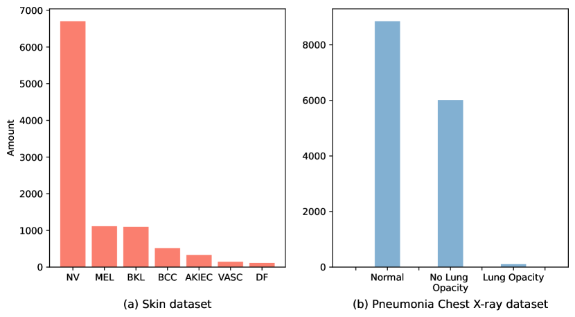
Convolutional Neural Networks (CNNs) are being widely used for image classification, object detection, segmentation, registration, and many other tasks in medical image analysis [1, 2]. With the help of CNNs, computer aided diagnosis systems can automatically recognize numerous diseases, such as breast malignancy classification [3], ear disease [4], skin lesion classification [5, 6], and skin cancer detection [7] and run on different devices [8]. Generally, images of common diseases are easier to collect, while images of rare diseases are not, which may lead to data imbalance issues for model training [9]. As shown in Figure 1, images from the major classes dominate the whole medical image dataset, while other classes consist of fewer images. That means a neural network is more likely to effectively learn the features of the common diseases than those of the rare diseases due to the very limited data of the latter classes, resulting in diagnosis bias towards the common diseases. To alleviate this data imbalance issue, we need to effectively handle the data imbalance between common diseases and rare ones [10, 11].

Figure 1: The imbalanced data distribution of two commonly used medical image datasets: (a) Skin dataset, and (b) Pneumonia Chest X-ray dataset. NV: Melanocytic nevus; MEL: Melanoma; BKL: Benign keratosis (solar lentigo/seborrheic keratosis/lichen planus-like keratosis); BCC: Basal cell carcinoma; AKIEC: Actinic keratosis/Bowen’s disease (intraepithelial carcinoma); VASC: Vascular lesion; DF: Dermatofibroma.

Several strategies have been proposed to address this problem, mainly focusing on how to effectively improve the classification performance of small sample classes. These strategies range from the input side of model training, such as balancing data between classes [12, 13], the model architecture, such as ensemble models [14, 15], to the output side of model training, such as setting different weights to different classes of training samples [12, 16]. Different from these existing studies, which consider each image as the basic unit and mainly focus on reweighting images or classes, a novel method called CARE (REgions of the lesion) is proposed here by delving into images and considering the high level semantics of images. Specifically, inspired by the process of human learning, attention was embedded into the learning process of CNN classifiers, particularly for rare diseases. By enabling classifiers to pay more attention to the lesion regions of minority class(es) during learning, the classifiers can learn disease characteristics more effectively from small samples of the minority classes. Due to limited training data for rare diseases, annotation of lesion regions from those images (in the form of bounding boxes containing lesion regions) does not usually take much effort for clinicians and thus is reasonably acceptable. Alternatively, lesion regions could be automatically estimated in advance based on state of the art saliency detection techniques DSR [17] and the segmentation model DeepLabV3 [18], as demonstrated in our study.

Also, different from existing attention relevant deep learning studies where attention is estimated as intermediate outputs of neural networks [19, 20], the proposed CARE framework novelly and explicitly uses attention as part of supervision signal (in addition to image labels) to help train the CNN classifiers. The proposed attention embedding mechanism does not alter neural network architectures and, therefore can be directly embedded into the training of any existing CNN architecture. What’s more, the proposed CARE is independent of any existing approach to data imbalance, and therefore can be combined to handle the imbalance issue together. Comprehensive experiments on a skin image dataset and a pneumonia chest X-ray dataset and with multiple CNN architectures showed that paying attention to lesion regions of rare diseases during learning did improve the classification performance on rare diseases.

It should be noted that a preliminary version of this work was presented at MIDL 2019 [21]. We further extend our work mainly in two folds. Firstly, extensive experiments are conducted to demonstrate the effectiveness of our proposed method. Our method is robust to the selection of hyperparameters designed in the loss. Secondly, our proposed method relies on bounding boxes for small classes, which were previously labeled by human experts.

Here we used two existing methods (DSR and DeepLabV3) to automatically detect bounding boxes [17, 18]. With the help of these automatically generated bounding boxes for the small class, our method still achieves comparable classification performance on the imbalanced dataset. Therefore, our method can be applied on datasets with severe data imbalance without the need of manual bounding boxes, thus reducing the annotation efforts of domain experts.

2 Related work

In this section, we briefly review existing work most relevant to our proposed approach, including the approaches to data imbalance issue and existing attention mechanisms.

2.1 Approaches to data imbalance issue

Multiple approaches have been proposed to solve the data imbalance issue. There are mainly three mainstreams: data rebalancing, class balanced loss, and transfer learning.

On the model input side, the data rebalancing idea has been widely used. For example, one traditional approach is to over-sample the limited data available for the small sample classes [22] or down-sample the data of the larger sample classes [23], thus generating a similar number of training examples for each class. Data augmentation, now a default choice for training deep neural networks, can also be used as an oversampling method to generate more data for small sample classes [24].

On the model output side, setting different weights for different training classes (class-level) or samples (sample-level) to balance loss was often used to handle the imbalance issue. At class-level reweighting training, cost sensitive learning is to improve the cost of misclassifying each training example coming from small sample classes, which can be easily realized by setting larger weights for small sample classes in the loss function [25]. In this way, different classes as a whole were treated equally in the cost calculation. Data imbalance issues could lead to the problem of inefficiency in utilizing examples from large classes. To tackle this challenge, the normal strategy is to adaptively reweight at the sample level. Focal loss reshapes the standard cross entropy by adaptively setting lower weights to easy samples and focusing on learning from hard samples [26]. Similarly, reweight training assigns weight to every sample depending on their gradient direction [27]. Based on such weights, hard negative mining can be adopted to select just a subset of training data for the next round training of classifiers [14]. Some studies show that metric learning, such as Siamese model [28] and triplet loss [29] can also perform well with imbalanced dataset.

Besides these approaches, another set of approaches focus on the model itself to alleviate the influence of data imbalance. Among this set, transfer learning via finetuning a pretrained classifier has been shown helpful to improve performance for both large and small sample classes [30, 31], and ensembling of multiple individual models has also become a routine to improve classification performance on each class [32]. Different from all the existing approaches, the proposed method in this study makes use of semantic information in terms of attention particularly in images of small sample classes to solve the imbalance issue.

2.2 Attention mechanisms

Attention mechanisms refer to those approaches which help models focus on more task relevant information during feature extraction from original data. The basic idea is to adaptively estimate the importance of each component (e.g., image feature of each local region) and then use the weighted components for further processing. Originally developed for machine translation tasks [19], attention mechanisms have been recently extended and applied in computer vision [33], e.g., with spatial attention in image captioning tasks [34], channel attention for image classification tasks [35], and self attention in video tasks [36]. In order to apply such attention mechanisms, the original neural network architecture would often be modified by embedding an attention module into the network model. Besides these approaches, another type of attention mechanism particularly in classification tasks, is to understand the decision process, by localizing and visualizing local image regions which contribute more to the final prediction. The well known methods include the Class Activation Map (CAM) [37] and its variants, such as Gradient-weighted Class Activation Mapping (Grad-CAM) [38]. CAM and Grad-CAM can be used to generate the heatmap of visualization of a region in an image that is most relevant to a specific prediction made by a CNN. The CAM approach utilizes the Global Average Pooling layer (GAP) to combine the feature maps of the final convolution layers and subsequently generates the heatmap through a linear combination of these maps. However, this methodology may be restricted when dealing with intricate networks containing numerous linear layers that succeed the last convolution layer. In contrast, Grad-CAM addresses this limitation by leveraging gradient information, which can be effortlessly acquired through backpropagation. However, the CAM variants were mainly developed for visualization purpose [39] and, therefore, didn’t seek to improve the classification or segmentation performance, since they are not directly involved in the training of neural network models. In our study, we take a different perspective and propose an attention based framework for training the neural network, which enables the resulting network being able to handle the data imbalance problem and improve the classification performance, especially on the class of smaller size.

3 Method

A study conducted in [40] showed that for medical students, during their training and learning process, lesions containing distinct characteristics of certain diseases were often shown and highlighted on the medical images, i.e., a kind of attention to task relevant regions. With the help of such attention to lesion regions, students probably can more effectively learn to grasp the distinct properties of each disease even with a small sample of medical images from that class. Inspired by the learning process of humans, here we propose a simple yet effective method to embed attention into the learning process of deep neural network classifiers for intelligent diagnosis.

3.1 Preliminary: Grad-CAM

A two-step process must be performed to generate a gradient-based class discriminative activation map $F^{c}\in\mathbb{R}^{u\times v}$ for any given class $c$. First, the feature maps $A\in\mathbb{R}^{d\times u\times v}$ are computed immediately after the last convolutional layer, followed by the Rectified Linear Unit (ReLU) in the CNN. Secondly, the gradient score $\sigma{{}^{c}}$ of each class $c$, $y^{c}$, with respect to feature map activation of the last convolution layer $A^{k}$, i.e., $\frac{\partial y^{c}}{\partial A^{k}}$, needs to be calculated.

Assuming the output of the final convolutional layer followed by ReLU is denoted by $A$, and the weight for the feature map of each channel (i.e., the last Linear Layer for ResNet50) is available, the final classification score $Y^{c}$ for a given class $c$ may be determined using the Equation (1).

$$Y^{c}=\sum_{k}\underbrace{w_{k}^{c}}_{\text{class feature weights }}\overbrace{\frac{1}{Z}\sum_{i}\sum_{j}}^{\text{global average pooling }}\underbrace{A_{ij}^{k}}_{\text{feature map }}$$ (1)

where $Z$ is the product of the height $u$ and width $v$ for each feature map $A_{k}$. For ResNet50 [41], used in our experiments, the feature map $A$ has $d=2048$ channels with a spatial size of $u=7$ and $v=7$. The weight $\sigma^{c}_{k}$ is calculated using the gradient computed from Equation (2).

$$\sigma_{k}^{c}=\overbrace{\frac{1}{Z}\sum_{i}\sum_{j}}^{\text{global average pooling }}\underbrace{\frac{\partial Y^{c}}{\partial A_{ij}^{k}}}_{\text{gradients via backprop }}$$ (2)

The gradient can be computed through the backpropagation process, regardless of how many intermediate linear layers are present between the last convolutional layer and the classification layer. This holds for architectures such as VGG19 [42], which contains two intermediate linear layers. The gradient-based class discriminative feature map for a given class $c$, denoted as $F^{c}$, can be defined by Equation (3) with gradient and feature map.

$$F^{c}=\sum_{k}\sigma_{k}^{c}A^{k}$$ (3)

In this study, we only focus on the true positive class’s feature map to simplify $F^{c}$ to $F$. We also normalize the feature map to the [0, 1] range and resize it back to [224, 224] for further attention loss computation. For clarity, we provide pseudocode for generating the feature map using Grad-CAM in Algorithm 1 in the Section 6 Appendix.

3.2 CARE: class attention to regions of lesions

We hypothesize that appropriate attention during learning would help neural network classifiers more effectively learn from small samples, particularly for rare diseases. Suppose the lesion regions of interest have been provided in advance for model learning, in the form of bounding boxes containing lesions. The human effort of providing bounding boxes is feasible for rare diseases because, quite often, only a small sample of images are available for each category, or alternatively, lesion regions could be automatically localized by saliency detection techniques (Section 3.3). Then, if there is a way to estimate the local regions on which the classifier focuses during image diagnosis, attention would be naturally embedded in those regions during classifier learning. Fortunately, such ‘visual focus’ of a classifier on any input image can be conveniently estimated by a recently proposed visualization approach Grad-CAM [38]. Given a well trained classifier and an input image, Grad-CAM can provide a class specific feature activation map in which regions with higher activation contribute more to the classifier’s output prediction being the specific class. Therefore, if the classifier attends to only the box bounded regions when diagnosing an image, the high activation regions from the Grad-CAM should also be within the bounded regions. In this sense, the spatial relationship (e.g., degree of overlap) between the high activation regions and the bounded image regions can be used to measure how well the classifier has attended to the bounded image regions.

Denote by $L_{a}$ the discrepancy between the high activation regions from Grad-CAM and the bounded image regions over all training data, then embedding attention during classifier learning can be realized by minimizing a new loss $L$ for the classifier,

$$L=(1-\alpha)L_{c}+\alpha L_{a}$$ (4)

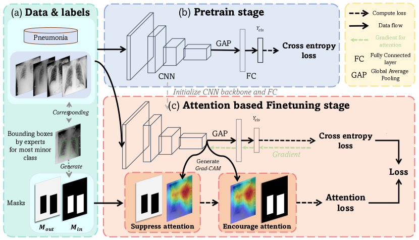
where $L_{c}$ is the general cross entropy loss for the network classifier, and $L_{a}$, called attention loss, which helps to drive the network to attend to box bounded image regions during training (Figure 2). $\alpha$ is a coefficient to balance the two loss terms. Considering the different influences of the inside box and outside box regions, the attention loss is further split into two items by

$$L_{a}=L_{in}+\lambda L_{out}$$ (5)

where the inner loss $L_{in}$ helps the classifier increase the attention inside the bounding box, and the outer loss $L_{out}$ helps the classifier decrease the attention outside the bounding box. $\lambda$ is a coefficient to balance the two loss terms. In detail, for any training image with bounding box(es) provided, let $M_{in}$ denote a binary complement image in which all pixels inside the bounding box are set to $1$ and others to $0$, and in contrast, $M_{out}$ denote a binary mask image in which all pixels inside the bounding box are set to $0$, and any pixel outside the box is set to either $1$ or a positive value relevant to the distance between the pixel and the bounding box. In our implementation, we simplify setting the pixel outside the bounding box to $1$, since we assume that the bounding boxes completely enclose the lesions and an attention map outside the boxes should always incur a penalty Let $F$ denote the normalized feature activation map from Grad-CAM for the training image based on the current classifier. Then $L_{in}$ and $L_{out}$ (for one training image) can be defined as

$$L_{in}=-\min(\frac{\Sigma_{i,j}M_{in}(i,j)\cdot F(i,j)}{\Sigma_{i,j}M_{in}(i,j)},\tau)$$ (6)

$$L_{out}=\frac{\Sigma_{i,j}M_{out}(i,j)\cdot F(i,j)}{\Sigma_{i,j}M_{out}(i,j)}$$ (7)

Here, $M_{in}(i,j)$ represents the value at the position $(i,j)$ in the mask $M_{in}$, and similarly for $M_{out}(i,j)$ and $F(i,j)$. Equation (7) represents the strength of feature activation outside the bounding box, while Equation (6) would penalize the classifier if the highly activated area inside the bounding box is not large enough (i.e., when the percent of the weighted activated area $\frac{\Sigma_{i,j}M_{in}(i,j)\cdot F(i,j)}{\Sigma_{i,j}M_{in}(i,j)}$ is smaller than a predefined threshold $\tau$). Note that for notation simplicity, Equations (6) and (7) are just for one single image. In fact, during training, the loss terms are calculated and averaged over all training images.

Figure 2: The framework of the proposed CARE method. Attention loss is designed to help the CNN model attend to lesion region for the minority category during model training. Bounding boxes representing lesions in images of only the minority category only need to be provided during training. The colorful heatmap is the activation map generated by Grad-CAM.

One advantage of the proposed attention based approach is its independence of model structures. Therefore the CARE can be directly embedded in the training processing of any existing CNN classifiers, without alternating their model architectures. Also, the CARE framework is independent of existing approaches to handling data imbalance, therefore, can be directly combined to further improve classification performance.

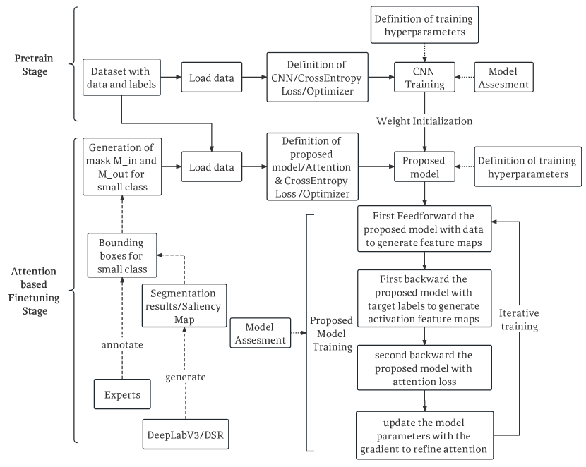
We also provide a diagram for clarifying the training process. The presented diagram in Figure 3 depicts the entirety of the process, encompassing data processing, model definition, and training methodology for the proposed model. The training of the proposed model, namely the CARE, can be categorized into two main stages: pretrain and attention based finetuning stages. The pretrain stage is used to pretrain the model for generating a reasonable attention map by Grad-CAM, and the attention based finetuning stage is trained with both the attention loss $L_{a}$ and the cross entropy loss $L_{c}$. During the pretrain stage, the CNN backbone and classifier are trained solely with data and corresponding labels. In the attention based finetuning stage, bounding boxes for the small class are generated via expert or automated techniques such as DSR and DeepLabV3, and subsequently processed to create training masks. The proposed model is then initialized with parameters from the pretrain stage and finetuned with the proposed attention loss alongside cross entropy loss. The initial feedforward and backward pass of the model produce an imprecise gradient-based class activation map. However, by utilizing the masks and a designed attention loss, attention outside the bounding boxes can be suppressed while directing attention toward the boxes, thus enabling the model to focus on the key aspects of the lesson. The full training process can be found in the pseudocode algorithm 2 in Section 6 Appendix.

Figure 3: Diagram of the proposed method. The diagram can mainly be divided into two stages, including the pretrain stage and attention based finetune stage.

3.3 Automatic generation of bounding boxes

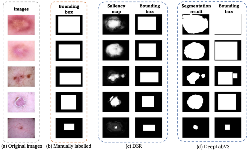
While lesion regions can be annotated by human experts, it would be ideal if lesion regions could be automatically localized without help from human experts. Here we provide two possible solutions to the automatic localization of lesion regions, at least for some medical classification tasks. The first one is based on saliency detection, which can estimate the salient regions of images without any annotation information [17]. In general, lesion regions often have a distinctive appearance (e.g., small darker regions in the image, as shown in Figure 4 compared to healthy backgrounds in images, and such distinctive appearance would be automatically found salient by saliency detection techniques. Since the output of saliency detection is often a probability map representing the degree of saliency at each pixel location, binarization of the saliency map is applied based on a fixed or adaptive threshold, after which the compact bounding boxes surrounding the binarized salient regions can be easily obtained (Figure 4). This study adopted a threshold value of 0.5, although the adaptive selection of the threshold could result in better performance.

Figure 4: Masks $M_{in}$ and $M_{out}$ generation for the small class based on DSR with post processing. CCL represents Connected Component Labeling.

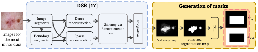
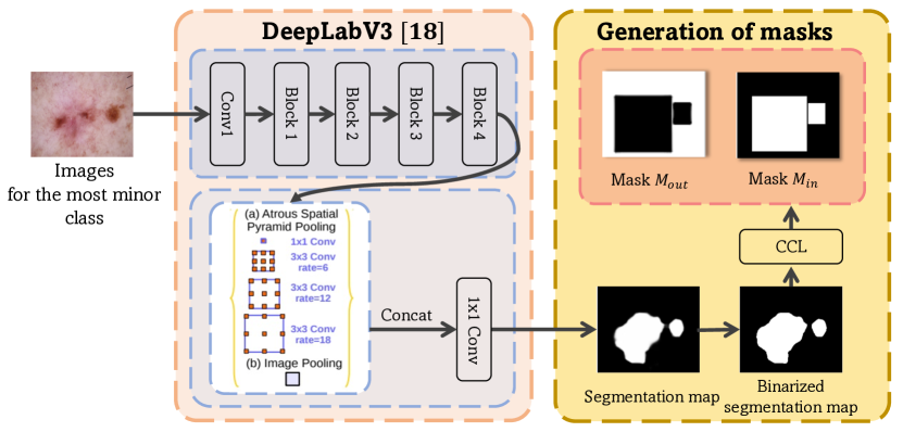
Similar to the process of saliency detection for bounding box generation, the lesion segmentation model could be trained in advance to automatically estimate possible lesion regions from a healthy background in images, but under the strong assumption that annotations of lesion regions are available for some images from the same training set or another similar data set. There are many similar datasets available with segmentation labels. To generate bounding boxes for the small class, we first use an existing yet related dataset to train a DeepLabV3 segmentation model with Dice Loss, stopping when the model converges. Once trained, as shown in Figure 5, we freeze the model’s parameters and use it to infer the data from the small class, producing a segmentation map where each pixel value ranges from 0-1. To obtain a binarized segmentation map, we further process the probability map with argmax. Lesion regions are identified as positive values, while 0 is considered background. To prepare the segmentation map for CARE, we use Connected-Component Labeling (CCL) [43, 44, 45] to remove small, unrelated lesions and obtain a rectangle containing the lesion. We set 1 for the lesion region and 0 outside the lesion region for the Mask $M_{in}$; the opposite process is followed for $M_{out}$. This process allows us to obtain the bounding boxes for the small class similar to human labeling. Compared to unsupervised saliency detection, supervised lesion segmentation is much more limited in bounding box generation.

Figure 5: Masks $M_{in}$ and $M_{out}$ generation for the most minor class based on lesion segmentation model (DeepLabV3) with post processing. CCL represents Connected Component Labeling.

4 Experiment

4.1 Experimental settings

4.1.1 Dataset

Two medical image datasets were used to evaluate the proposed approach. One is the Skin Dataset provided by the ISIC2018 Challenge with seven disease categories [46], in which 6705 images are for Melanocytic nevus and only 115 images for Dermatofibroma, clearly having serious data imbalance among classes. One bounding box was generated for each image of the rare disease Dermatofibroma by the author and confirmed by a dermatologist. The other is the Pneumonia detection X-ray dataset with three categories , including 8,851 ‘Normal’ images, 105 ‘Lung Opacity’ images, and 6,012 images of ‘No Lung Opacity/Not Normal’. Each ‘Lung Opacity’ image was provided with one or multiple bounding boxes indicating the region of pneumonia. Although the original objective of this Chest X-ray data is for lesion detection, we used it for 3 class classifications, with the ground-truth bounding boxes used to evaluate the proposed approach. The number of ‘Lung Opacity’ images is much smaller than the other two categories, being considered as the minority class in a data imbalance scenario. All images were resized to $224\times 224$ pixels, with bounding boxes resized accordingly for the small sample class in each dataset. For each dataset, images are randomly split into a training set (80%) and a test set (20%) with stratification.

In the experiments, the training of CARE is divided into two stages. In the pretrain stage , each backbone CNN classifier (i.e., the branch without the attention loss in Figure 2) used was pretrained firstly on ImageNet and then on the training set without the attention loss. The training at this stage is stopped when the cross entropy loss does not decrease anymore (normally within 200 epochs in our experiment). In the attention based finetuning stage, attention loss was included to finetune the pretrain stage ’s classifier with the training set. $\alpha$ in Equation(4) was set to 0.5 unless otherwise mentioned. AdamW optimizer [47] was used in all experiments , with an initial learning rate set at $0.0001$. $\lambda$ was empirically set to 0.5 for the X-ray dataset and 1.0 for the Skin dataset. More details of experimental settings were summarized in Table 1 for the pretrain and finetuning stages . In testing, each test image (without any bounding box) was fed to the CNN classifier for prediction. Note that the CARE approach needs no bounding box in testing.

Table 1: Details of experimental setting on the Skin dataset. ‘-’ denotes that the hyperparameter is not used in the pretrain stage .

Config	Learning Rate	Batch Size	Epochs	Activation Feature Map	$\alpha$	$\lambda$	$\tau$
Pretrain Stage	1e-4	96	200	-	-	-	-
Finetune Stage	1e-4	96	200	$224\times 224$	0.5	1	0.7

To evaluate the performance of the proposed CARE, two evaluation metrics suggested by the ISIC2018 Challenge were used here, including mean class accuracy (MCA, i.e., average recall over all classes, treating contributions from each class equally) [22] and the area under the ROC curve (AUC) [48, 49]. Since AUC is general for binary classification, here for multi class classification tasks, AUC was first calculated for each class (treating all the other classes as a negative class) and then averaged. Besides, we use Recall for the smallest class (i.e., Dermatofibroma in Skin Dataset, and Lung Opacity in the Pneumonia dataset) to particularly highlight the performance of classifiers on the small sample class.

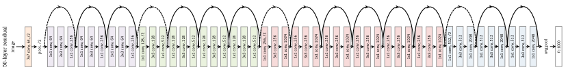
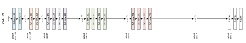
The architectures of the backbone used in our experiments like ResNet50 [41] and VGG19 [42] can be found in Figure 6 and Figure 7, respectively.

Figure 6: Architecture of the ResNet50 [41] backbone.

Figure 7: Architecture of the VGG19 [42] backbone.

4.2 Effectiveness of the proposed CARE

4.2.1 Baseline and comparison

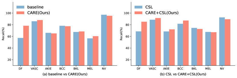
To test the effectiveness of the proposed approach, we compared CARE to three widely used strategies for handling data imbalance on both datasets, namely, 1) cost sensitive learning denoted by CSL [12], 2) focal loss denoted by FL [26], a representative method of hard negative mining, and 3) data augmentation (including rotation, flip and color jitter) denoted by DA [24]. We further tested our approach by embedding CARE into the three strategies, resulting in methods of CARE+CSL, CARE+FL, and CARE+DA. We also tested a baseline without using the visual attention loss in Figure 2. Table 2 shows the comparison results on Pneumonia and Skin datasets with MCA and AUC, and on small classes with Recall. It can be observed that CARE outperforms the baseline significantly in terms of Recall, AUC, and MCA, in particular with a large margin on recall for the small sample class (31.1% vs. 7.4% on the Pneumonia dataset, and 73.9% vs. 52.2% on the Skin dataset). All three strategies (i.e., CSL, FL, and DA) perform better than the baseline without any treatment of data imbalance, which is expected. It is worth highlighting that adding CARE to each of CSL, FL or DA can boost the performances significantly w.r.t the use of each method alone; for instance, the Recall, AUC, and MCA of CARE+CSL on the Pneumonia dataset are respectively 45.0%, 0.769 and 65.2%, significantly better than CSL only. For the CSL method, additional experiments showed that varying loss coefficients for the minority class did not change the finding, i.e., CARE+CSL always performs better than CSL alone. This indicates that our approach is capable of boosting their performances significantly when plugged into the existing strategies for handling data imbalance. Figure 8 demonstrates the detailed classification performance of each class. Compared with each baseline in Figure 8 (a) and (b) , our CARE method consistently improves the classification performance on minority classes (e.g., DF, VASC) while often slightly decreasing the performance on majority classes (e.g., NV, BKL). It has been widely observed in literature [50] on imbalanced classification that the performance of one or a few majority classes would often become decreased a bit in accompanying the increased performance of minority classes.

Table 2: Comparison between baselines and our method on the two commonly used imbalanced medical image datasets with backbone ResNet50.

Method	Pneumonia dataset			Skin dataset
	Recall of the most minor class	AUC	MCA	Recall of the most minor class	AUC	MCA
baseline	7.4	0.663	56.8	52.2	0.962	74.1
CARE (ours)	31.1	0.741	63.3	73.9	0.973	78.2
CSL	11.1	0.704	57.9	56.5	0.981	77.2
CARE+CSL(ours)	45.0	0.769	65.2	65.2	0.986	81.0
FL	11.1	0.758	58.4	52.2	0.918	71.5
CARE+FL (ours)	49.4	0.769	66.7	60.9	0.933	73.9
DA	20.1	0.805	59.6	56.6	0.862	54.4
CARE+DA(ours)	45.2	0.796	66.0	60.3	0.885	56.2

Figure 8: Comparison between baselines and our method in each class on the Skin dataset.

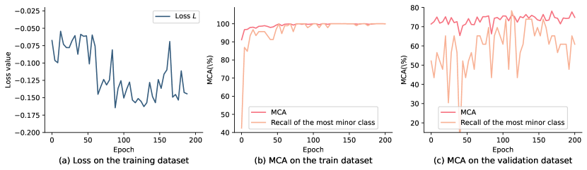
In Figure 9, we illustrate the training process of the CARE(Ours) model on the Skin dataset (2nd row in Table 2) as an example. The table presents the loss curve, MCA curve, and recall of the most minor class on the training dataset, as well as the MCA and recall of the most minor class on the validation dataset. Figure 9 (a) shows that the loss decreases as the training process advances. Figure 9 (b) indicates that it may take up to 200 epochs for the model to converge and fit well on all data across all classes. Figure 9 (c) suggests that training the model for more epochs can enhance the recall of the most minor class significantly, and MCA increases. However, due to the dataset’s severe imbalance, the training curve may not be as stable as other balanced datasets, which is widely observed [50].

Figure 9: The training process details for the CARE(Ours) in Table 2. (a) displays the changes in the total loss throughout the training process. (b) shows the changes in the MCA and recall of the most minor class on the training dataset during the training process. (c) presents the changes in the MCA and recall of the most minor class on the validation dataset.

In addition, two well known data imbalance strategies Siamese [28]  and Decouple [51] were adopted for comparison on the Skin dataset. The decoupling method [51] is a representative SOTA strategy dealing with data imbalance and has been re-implemented here. In detail, following the work [51], we freezed the parameters of the first 7 layers except for the last convolution block and classifier. As shown in Table 3, our proposed method boosts both methods, particularly on the small class DF and the overall classification performance over all classes.

Table 3: Comparison with the Siamese and the Decoupling methods on the Skin dataset.

Method	MCA	Recall
		DF	VASC	AKIEC	BCC	PBK	MEL	NV
Siamese	56.9	21.7	51.7	53.0	67.9	60.0	45.7	98.3
Siamese+CARE(ours)	68.9	65.2	68.9	48.4	70.8	65.4	70.8	93.8
Decouple	73.9	65.2	82.7	57.5	81.5	76.3	63.2	91.9
Decouple+CARE (ours)	78.3	73.9	89.6	62.1	83.4	74.0	73.0	92.2

4.2.2 Visual inspection

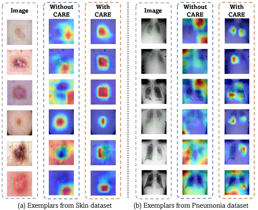
To show the effect of the proposed attention loss, we visualize the classification activation maps of sample test images from both datasets in Figure 10 (a) and (b). For clarity, we also superimpose (ground truth) bounding boxes highlighting the lesion regions on the test images, provided along with the dataset (the Pneumonia dataset) or in-house annotation (the Skin dataset). Note that we did not use any of those bounding boxes during testing, but here merely for visualization purposes. It can be observed that the activated regions (red regions in the second column of the Figure 10 (a) and the second column of Figure 10 (b) ) without using the proposed attention loss (Eq. 5) were deviated from or not focused on lesion regions, while those ( third column of Figure 10 (a) and last columns of Figure 10 (b) ) produced by CARE localized the lesion regions well. These results on the test images reveal that the CARE model could have learned to focus on lesion regions when analyzing new images, through attention loss optimized during training. On the other hand, as shown in the last two rows of Figure 10(b), CARE did not always help the model focus on the annotated lesion region. However, compared with the results without CARE (second last column), CARE help the model focus on more reasonable areas like the chest and heart where the shape and texture of the area look very similar to the actual lesion. This again indicates that CARE tries to help the model capture the actual lesion to make the classification decision. We found that failure cases more likely appear in the Pneumonia dataset than the Skin dataset, probably because the actual lesions in the Pneumonia dataset are relatively small and often similar to other image regions. Replacing Grad-CAM with a more precise class activation map generation method during model training could improve the model’s performance.

Figure 10: Visualization of activation maps with and without using CARE on (a) the Skin Dataset and (b) the Pneumonia Dataset. First column: test images superimposed with bounding boxes; the Second and third columns: activation maps without and with CARE attention loss, respectively. Similarly for the last three columns. We use Grad-CAM to estimate class activation maps (best viewed in color)

4.3 Robustness of CARE

4.3.1 Flexibility with model architecture

Our proposed CARE framework is independent of model structures. To show this, we tested variants of our CARE framework built with two different widely used CNN architectures: ResNet [41] and VGG19 [42]. For ResNet, we further tested the different number of layers (18, 50, and 152 layers), from shallow to very deep. VGG19 uses a 19 layered structure. Thus in total, we have four backbones of CNN architectures: ResNet18, ResNet50, ResNet152, and VGG19. With each backbone, we compared the performance of the resulting CARE model (denoted by X(CARE), with X representing the name of the backbone) and the original backbone network. From Table 4, it can be observed that different original backbone architectures perform differently, among which VGG19 performs the best. For each of the backbone, its CARE version consistently outperforms the original network in terms of both recall and MCA. This confirms the flexibility of the proposed CARE in the combination of various model architectures.

Table 4: Performance of CARE with various model architectures on two commonly used imbalanced medical image datasets. X(CARE) means that the CARE has the backbone X, e.g., ResNet18(CARE) represents the CARE with the backbone model ResNet18. It’s worth noting that all models apply CSL in this table.

Backbone	Pneumonia dataset			Skin dataset
	Recall of the most minor class	AUC	MCA	Recall of the most minor class	AUC	MCA
ResNet18	15.2	0.581	57.8	60.9	0.990	74.1
ResNet18(CARE)	25.5	0.710	58.8	73.9	0.969	76.2
ResNet50	11.1	0.704	57.9	56.5	0.953	77.7
ResNet50(CARE)	45.0	0.769	65.2	65.2	0.986	81.0
ResNet152	11.4	0.747	59.1	61.9	0.914	80.5
ResNet152(CARE)	31.3	0.749	63.8	72.2	0.966	81.9
VGG19	25.8	0.873	61.7	47.8	0.881	70.2
VGG19(CARE)	41.2	0.871	64.3	56.5	0.933	72.8

4.3.2 Tolerance to bounding box accuracy

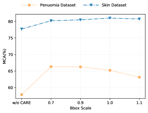
It is noted that the training of our model needs bounding box annotations for the smallest class. For many rare or uncommon diseases (such as Dermatofibroma in this study), the bounding box annotation effort for the lesion regions in the minority class is usually very small compared to that of accurate boundary pixel level annotations. Even though, there might exist inter- or intra-observer variations in annotation. The bounding boxes used thus far are tightly around the lesion region. To relax this requirement, we vary the bounding boxes by scaling at 0.7, 0.9, 1.0, and 1.1, and test the robustness of our approach to such scaling. In detail, we utilized manually labeled bounding boxes as the reference with a scale of 1.0 and varied the size of the bounding boxes that covered the lesion region using different ratios before feeding the model. Specifically, we increased and decreased the size of the original bounding box that encompasses the lesion area by factors of 0.7 to 1.1 to either encompass a smaller or larger region of the lesion in the images. . Figure 11 shows the performance of our model at different scaling. It can be seen that the performance remains stable when the box size changes within a reasonable range, for instance, from 0.7 to 1.1. This indicates that our approach is largely tolerant to the sizes of bounding boxes, i.e., the bounding boxes do not need to be tight around the lesions, with the flexibility of using a looser bounding box, which would require less annotation effort from human experts.

Figure 11: Robustness to scales of bounding box, tested with ResNet50(CARE) on the Skin dataset.

4.3.3 Effect of $\alpha$

We further conducted a set of experiments to evaluate the effect of the coefficient parameter $\alpha$ of the attention loss term using ResNet50(CARE), and the results are shown in Table 5. It can be observed that the performance of the model remains consistently better than the baseline (with $\alpha=0$) when $\alpha$ changes within a reasonably large range, for instance, from 0.3 to 0.9, and particularly the MCA performance remains stable with varying $\alpha$ values on both datasets. This indicates that our model is insensitive to the choices of the value of $\alpha$ in improving the classification performance.

Table 5: Effect of the coefficient $\alpha$ on classification performance with ResNet50(CARE). Note that all models here apply CSL.

$\alpha$	Pneumonia dataset		Skin dataset
	Recall of the most minor class	MCA	Recall of the most minor class	MCA
0	11.1	57.9	56.5	77.7
0.1	28.8	63.8	55.2	78.8
0.3	38.3	64.4	65.2	79.9
0.5	45.0	65.2	65.2	80.3
0.7	42.6	64.3	65.2	80.2
0.9	50.7	65.2	65.1	80.2

4.3.4 Effect of $\tau$

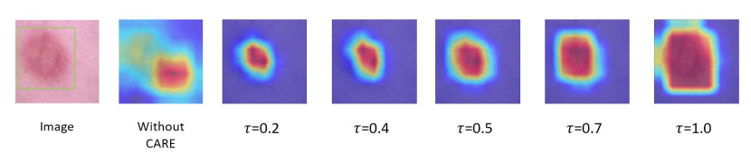
In addition, the effect of the threshold hyperparameter $\tau$ in the loss term $L_{in}$ was evaluated by varying its values from 0.2 to 1.0 with the ResNet50(CARE). Table 6 shows that, although the classification performance vary with different threshold values, they all outperform the baseline model (without using CARE). Figure 12 shows with increasing value of the threshold, the model would be trained to attend to larger lesion regions during diagnosis, which is as expected and confirms the role of the loss term $L_{in}$. $\tau$ is a threshold to discourage the attention to fulfill the whole bounding box. Since lesions of some diseases such as Skin tumors may occupy most of the bounding box, and some other diseases may only occupy a relatively smaller area within the bounding box indicating a smaller $\tau$ should be used, the choice of $\tau$ may be different on different datasets. This sensitivity study shows that model performance remains stably high within a large range of $\tau$ values on both datasets. In practice, $\tau$ was empirically set based on a small internal validation set from each dataset, and many other choices would result in similar performance based on the sensitivity study.

Table 6: Effect of the hyper-parameter $\tau$ on classification performance.

$\tau$	Penuomia Dataset		Skin Dataset
	Recall of the most minor class	MCA	Recall of the most minor class	MCA
baseline	11.1	57.9	56.5	77.7
0.2	33.3	64.9	73.9	79.1
0.4	51.8	68.9	69.6	78.8
0.5	45.0	65.2	65.2	81.0
0.7	51.9	67.4	65.2	80.2
1	37.0	64.0	78.3	79.6

Figure 12: Exemplar effect of the hyper-parameter $\tau$. Higher $\tau$ values cause larger attended regions on the test image.

4.3.5 Effect of $\lambda$

For the coefficient $\lambda$, Table 7 shows that, when $\lambda$ varies from 0.7 to 1.3 (2nd to 4th rows), the model achieves similar high performance in MCA over all classes and improved performance in recall for the smallest class DF, again confirming the robustness of the proposed method.

Table 7: Effect of the coefficient $\lambda$ on classification performance on the Skin dataset. The 1st row represents the results of CSL without CARE.

$\lambda$	MCA	Recall
		DF	VASC	AKIE	BCC	PBK	MEL	NV
-	75.9	56.5	93.1	66.6	80.5	76.8	64.1	94.0
0.7	79.95	60.8	96.5	78.7	87.3	76.8	67.2	92.0
1.0	80.6	86.9	89.6	72.7	86.4	68.1	71.7	88.2
1.3	79.94	69.5	96.5	68.1	88.3	70.4	78.4	87.9

4.4 CARE with automated bounding box generation

This experiment tests whether automatically estimated bounding boxes would also help improve the classification performance on the small sample class of skin images. While there exist multiple solutions to automatic bounding box generation, here as two examples, we adopted a traditional unsupervised saliency detection method DSR [52] and a well known supervised segmentation model DeepLabV3 [18]. To use the segmentation model in our CARE method, we need to train a segmentation model using certain dermoscopic image dataset, with lesion region annotations. Here the Skin dataset from the ISIC2018 Skin Segmentation Challenge, which includes 2,594 dermoscopic images with lesion region annotations, was used to train the DeepLabV3 model. It is important to note that this dataset is different from the skin disease types used for the classification task but is still appropriate for our CARE method since these images share similar edge and texture features and backgrounds. Note that all the small class images used for classification were not included in the segmentation training set. Figure 13 shows examples of bounding boxes automatically generated by the two methods.

Figure 13: Automated generation of bounding boxes for the minority class in the Skin Dataset. From left to right: (a) original image, (b) manually labeled bounding box, (c) saliency map by DSR, bounding box based on DSR, (d) segmentation result by DeepLabV3, bounding box based on segmentation.

With the automatically estimated bounding boxes, the two models trained by the CARE framework, i.e., CARE(DSR) and CARE(DeepLabV3) with the backbone ResNet50 in Table 8, outperform the baseline model without using CARE, particularly on the smallest class. This confirms the effect of the CARE framework on performance boosting even with automatically estimated bounding boxes. It can also be observed from Table 8 that the network model CARE(GT) trained with the manually labeled bounding boxes performs the best. Figure 14 shows the corresponding visualization results.

Table 8: Performance of CARE models on the Skin Dataset, with bounding boxes from different ways. CARE(X) denotes the CARE model with bounding boxes from X.

Method	Baseline	CARE(GT)	CARE(DSR)	CARE(DeepLabV3)
MCA	74.13	78.17	77.02	75.61
Recall of the most minor class	52.17	73.91	65.22	60.87

Figure 14: Visualization of activation maps with different versions of CARE. From first to last column: (a) original images superimposed with bounding boxes, (b) activation maps without using CARE attention loss, (c) activation maps with CARE(GT), (d) CARE(DSR), and (e) CARE(DeepLabV3), respectively. We use Grad-CAM to generate the class activation maps (best viewed in color).

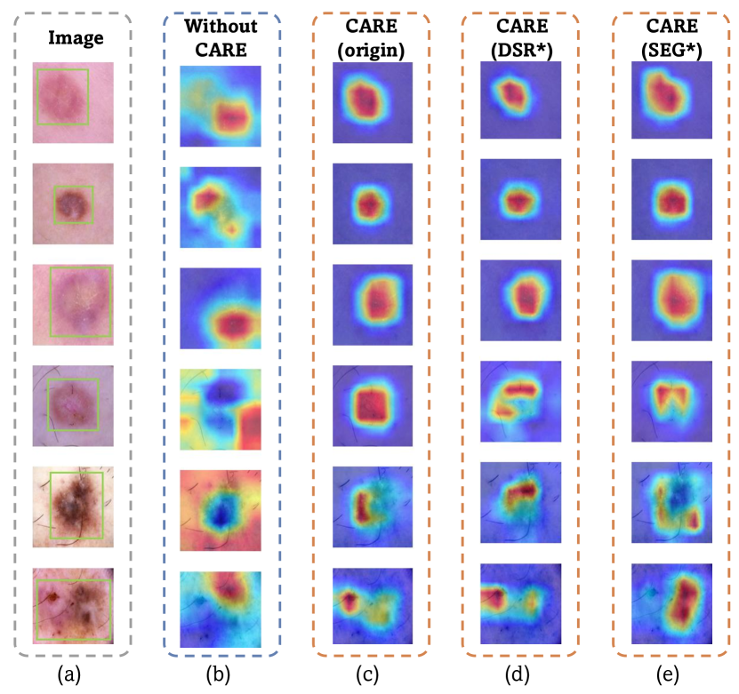
This is reasonable because the manually labeled bounding boxes are often more accurate and less erroneous compared to those by the saliency detection or segmentation methods. As part of future studies, better methods of estimating lesion regions could be developed and applied here. The visual illustration in Figure 14 also shows that the network models trained with automatically estimated bounding boxes ( Figure 14 (d) and (e) ) can also well attend to lesion regions during diagnosis, although sometimes the attention is slightly worse ( Figure 14 (d) ) than that from the network model trained with the manually labeled bounding boxes ( Figure 14 (a) ).

Similar to the above tests of combining the CARE framework with existing approaches to data imbalance issue (Table 2), Table 9 clearly shows that using the automatic generated bounding boxes, the combination of CARE with CSL or FL also significantly improved the performance of the network model trained with CSL or FL alone. In particular, the improvement on the smallest class (Recall) is more significant. This further supports that even with the possibly inaccurate estimation of bounding boxes, the CARE framework is effective to further improve classification performance when combined with existing data imbalance strategies.

Table 9: Performance of the ResNet50 models on the skin dataset when trained in the CARE framework together with CSL (Cost Sensitive Learning) and FL (Focal Loss) respectively. Bounding boxes used in CARE were estimated by the saliency detection method DSR or the segmentation model DeepLabV3.

Method	CSL	CSL+ CARE(DSR)	CSL+ CARE(DeepLabV3)	FL	FL+ CARE(DSR)	FL+ CARE(DeepLabV3)
MCA	77.7	80.2	81.4	72.0	72.3	74.6
Recall of the most minor class	56.5	78.3	86.7	52.2	60.9	82.6

4.5 Increasing classes of masks in CARE

The algorithm is not limited to the class with the smallest sample size. The three smallest categories of the Skin dataset are DF, VASC, and AKIEC, respectively, having 115, 142, and 327 images. Segmentation model DeepLabV3 was used to generate masks for the three classes of training data, and the generated masks were double checked by medical experts to ensure most masks were reasonably good enough. As shown in Table 10, applying the proposed method to DF, DF+VASC, and DF+VASC+AKIEC can clearly improve the recall of the small classes (56.52$\rightarrow$89.96, 89.65$\rightarrow$96.55, 68.18$\rightarrow$74.24) and the MCA over all classes compared to the baseline (cost sensitive learning, CSL). It can also be observed that the performance improvement on the smallest class DF becomes smaller when masks are provided for the other small (but relatively larger) classes VASC and AKIEC, during model training. This is probably because attention is biased toward the relatively larger classes VASC and AKIEC during model training by our CARE method.

Table 10: Performance of CARE when masks were provided for different number of minority classes. In this table, CARE [X] means the masks were provided for the disease(s) X when the proposed CARE method was used for model training.

Method	MCA	Recall
		DF	VASC	AKIEC	BCC	BKL	MEL	NV
CLS (Baseline)	$77.69$	$56.52$	$89.65$	$68.18$	$90.29$	$75.45$	$71.17$	$92.54$
CARE [DF]	$\mathbf{81.35}$	$\mathbf{86.96}$	$89.66$	$66.67$	$88.35$	$76.82$	$68.47$	$92.54$
CARE [DF+VASC]	$80.51$	$82.61$	$\mathbf{96.55}$	$66.67$	$86.41$	$74.09$	$64.41$	$92.84$
CARE [DF+VASC+AKIEC]	$80.28$	$69.57$	$89.66$	$\mathbf{74.24}$	$90.29$	$76.82$	$68.92$	$92.46$

5 Conclusions

In this study, we proposed a simple yet effective learning framework CARE to handle the data imbalance issue in medical image diagnosis. The attention mechanism is embedded into the CNN learning process for the minority category, helping the CNN focus on the right lesion region during learning and thus improving the classification accuracy for the minority class. CARE uses Grad-CAM to estimate attention maps and bounding boxes to indicate proper lesion regions of minority categories. This method can be applied to any CNN based classifier without altering neural network architectures. To alleviate the need for manual annotations of those bounding boxes, we further proposed variants of CARE with comparable performance. Comprehensive experiments have been performed on two commonly used imbalanced medical image datasets, showing that the proposed method can help the classifier improve the classification performance, particularly for the minority classes. Models trained together with CARE have a $2.5\text{-}4\%$ improvement on the Skin dataset and $6.4\text{-}8.3\%$ improvement on the Pneumonia dataset in mean class accuracy, and $4\text{-}21\%$ improvement on the smallest class of the Skin dataset and $25\text{-}38\%$ improvement on the smallest class of the Pneumonia dataset in the recall. CARE can also combine with different existing data imbalance strategies to further boost their performances, demonstrating its flexibility.

The proposed CARE method can be improved from the following aspects. First, CARE is a two-stage method in which the mask information is used only in the second stage to fine-tune the model. In future work, we will investigate an end-to-end learning framework in which the mask information can be simultaneously estimated together with model training. Since there may be small lesions, we believe that replacing Grad-CAM with a more precise method for generating activation maps could improve the model’s performance. Second, CARE is mainly designed for CNN models. Considering that the recently proposed Capsule network [53, 54, 55] and vision Transformer [56, 57] models can well capture spatial relationships of learned local features and have been successfully applied to image classification, it is interesting to extend the proposed CARE method to such model backbones in future work. While the proposed method showed promising results for the smallest class, applying CARE to multiple classes showed a decrease in recall for those classes with smaller sample sizes. In addition, the CARE method is currently applied to two image classification tasks only. Its potential usage in more medical diagnosis applications and other medical image analysis tasks like lesion detection could be further investigated.

6 Appendix

Algorithm 1 Pseudocode of generation of feature maps in PyTorch-like style.

  # feature_map: the activation feature map $A$ with the shape of [2048, 7, 7]

  # grad_class: the gradient score of class score $Y^{c}$ with respect to the activation feature map, with the shape of [2048, 7, 7], which can be obtained by backpropagation.

  

  def get_gradCAM(feature_map, grad_class):

    channels, height, width = grad.size()

    grad = mean(grad, dim=[1, 2])

    weight = grad.reshape(channels, 1, 1)

    feature_map = weight * feature_map

    grad_cam = sum(feature_map, dim=0)

    grad_cam = grad_cam.reshape(7, 7)

    return grad_cam

  

  # Normalize the feature map to the range of [0-1] and resize from [7, 7] to [224, 224].

  def post_process(grad_cam):

    grad_cam -= min(grad_cam)

    grad_cam /= max(grad_cam)

    grad_cam = interpolate(grad_cam, size=(224, 224), mode=’bilinear’)

    return grad_cam

Algorithm 2 Pseudocode of CARE in PyTorch-like style.

  # loader_m: dataloader with masks for the small class

  # loader: dataloader without masks for the small class

  # m_p, m_f: model respectively for the pretrain stage and the (attention based) finetune stage

  # $\alpha$, $\lambda$, $\tau$: hyperparameters

  

  # the pretrain stage

  for epoch in range(n_epochs):

    for x, labels in loader: # load a minibatch x and labels with N samples

      x = aug(x)

      logits = m_p.forward(x)

      # pre-train with weighted cross-entropy loss

      loss = CrossEntropyLoss(logits, labels)

      loss.backward()

      update(m_p)

  

  # the (attention based) finetune stage

  m_f.params = m_p.params # initialize with parameters from the pretrain stage

  m_f.register_hook() # Register function to store feature map and gradient score.

  for epoch in range(n_epochs):

    # load a minibatch x, Mask M and labels. Masks are only for the small class

    for x, M, labels in loader_m:

      x, M = aug(x, M) # augmented with the same operation

      logits, feature_map = m_f.forward(x)

      # finetune with weighted cross-entropy loss

      $L_{c}$ = (1-$\alpha$) * CrossEntropyLoss(logits, labels)

      # generate feature map F by Grad-CAM style

       $L_{c}$.backward(retrain_graph=True)

      grad_class = m_f.get_gradients() # gradient score with respect to feature map

      F = get_gradCAM(feature_map, grad_class) # obtain Grad_CAM, and defined in Algorithm 1

      F = post_process(F) # Defined in Algorithm 1

      if M is not empty:

        $L_{in}$ computed by Equation (3) in Section 3.1

        $L_{out}$ computed by Equation (4) in Section 3.1

        $L_{a}=L_{in}+\lambda L_{out}$

      else:

        $L_{a}=0$

      $L_{a}*=\alpha$

      $L_{a}$.backward()

      update(m_f)

References

- [1] S. M. Anwar, M. Majid, A. Qayyum, M. Awais, M. Alnowami, M. K. Khan, Medical image analysis using convolutional neural networks: a review, Journal of Medical Systems 42 (2018) 1–13.
- [2] D. Shen, G. Wu, H.-I. Suk, Deep learning in medical image analysis, Annual Review of Biomedical Engineering 19 (2017) 221–248.
- [3] C. Haarburger, M. Baumgartner, D. Truhn, M. Broeckmann, H. Schneider, S. Schrading, C. Kuhl, D. Merhof, Multi scale curriculum cnn for context-aware breast mri malignancy classification, in: Proceedings of the International Conference on Medical Image Computing and Computer Assisted Intervention, 2019, pp. 495–503.
- [4] M. Viscaino, M. Talamilla, J. C. Maass, P. Henríquez, P. H. Délano, C. Auat Cheein, F. Auat Cheein, Color dependence analysis in a cnn-based computer-aided diagnosis system for middle and external ear diseases, Diagnostics 12 (4) (2022) 917.
- [5] E. Goceri, A. A. Karakas, Comparative evaluations of cnn based networks for skin lesion classification, in: Proceedings of the International Conference on Computer Graphics, Visualization, Computer Vision and Image Processing, 2020, pp. 1–6.
- [6] E. Göçeri, Convolutional neural network based desktop applications to classify dermatological diseases, in: Proceedings of the International Conference on Image Processing, Applications and Systems, IEEE, 2020, pp. 138–143.
- [7] E. Goceri, Automated skin cancer detection: where we are and the way to the future, in: 2021 44th International Conference on Telecommunications and Signal Processing, IEEE, 2021, pp. 48–51.
- [8] E. Goceri, Diagnosis of skin diseases in the era of deep learning and mobile technology, Computers in Biology and Medicine 134 (2021) 104458.
- [9] R. C. Griggs, M. Batshaw, M. Dunkle, R. Gopal-Srivastava, E. Kaye, J. Krischer, T. Nguyen, K. Paulus, P. A. Merkel, et al., Clinical research for rare disease: opportunities, challenges, and solutions, Molecular Genetics and Metabolism 96 (1) (2009) 20–26.
- [10] E. Goceri, Image augmentation for deep learning based lesion classification from skin images, in: Proceedings of the International Conference on Image Processing, Applications and Systems, IEEE, 2020, pp. 144–148.
- [11] C. Yoon, G. Hamarneh, R. Garbi, Generalizable feature learning in the presence of data bias and domain class imbalance with application to skin lesion classification, in: Proceedings of the International Conference on Medical Image Computing and Computer Assisted Intervention, 2019, pp. 365–373.
- [12] Y. Sun, M. S. Kamel, A. K. Wong, Y. Wang, Cost-sensitive boosting for classification of imbalanced data, Pattern Recognition 40 (12) (2007) 3358–3378.
- [13] M. M. Rahman, D. N. Davis, Addressing the class imbalance problem in medical datasets, International Journal of Machine Learning and Computing 3 (2) (2013) 224.
- [14] C. Li, Classifying imbalanced data using a bagging ensemble variation, in: Proceedings of the Annual Southeast Regional Conference, 2007, pp. 203–208.
- [15] S. Wang, X. Yao, Diversity analysis on imbalanced data sets by using ensemble models, in: Proceedings of the Annual Southeast Regional Conference, 2009, pp. 324–331.
- [16] P. Domingos, Metacost: A general method for making classifiers cost-sensitive, in: Proceedings of the ACM SIGKDD International Conference on Knowledge Discovery and Data Mining, 1999, pp. 155–164.
- [17] X. Li, H. Lu, L. Zhang, X. Ruan, M.-H. Yang, Saliency detection via dense and sparse reconstruction, in: Proceedings of the IEEE International Conference on Computer Vision, 2013, pp. 2976–2983.
- [18] L.-C. Chen, G. Papandreou, F. Schroff, H. Adam, Rethinking atrous convolution for semantic image segmentation, arXiv preprint arXiv:1706.05587 (2017).
- [19] A. Vaswani, N. Shazeer, N. Parmar, J. Uszkoreit, L. Jones, A. N. Gomez, Ł. Kaiser, I. Polosukhin, Attention is all you need, in: Proceedings of the Advances in Neural Information Processing Systems, 2017, pp. 5998–6008.
- [20] K. Xu, J. Ba, R. Kiros, K. Cho, A. Courville, R. Salakhudinov, R. Zemel, Y. Bengio, Show, attend and tell: Neural image caption generation with visual attention, in: Proceedings of the International Conference on Machine Learning, 2015, pp. 2048–2057.
- [21] J. Zhuang, J. Cai, R. Wang, J. Zhang, W. Zheng, Care: Class attention to regions of lesion for classification on imbalanced data, in: Proceedings of the Medical Imaging with Deep Learning, 2019, pp. 588–597.
- [22] N. V. Chawla, K. W. Bowyer, L. O. Hall, W. P. Kegelmeyer, Smote: synthetic minority over-sampling technique, Journal of Artificial Intelligence Research 16 (2002) 321–357.
- [23] R. C. H. Chris Drummond, C 4 . 5 , class imbalance , and cost sensitivity : Why under-sampling beats oversampling, 2003.
- [24] L. Perez, J. Wang, The effectiveness of data augmentation in image classification using deep learning, arXiv preprint arXiv:1712.04621 (2017).
- [25] S. H. Khan, M. Hayat, Bennamoun, F. Sohel, R. B. Togneri, Cost-sensitive learning of deep feature representations from imbalanced data, IEEE Transactions on Neural Networks and Learning Systems 29 (2015) 3573–3587.
- [26] T.-Y. Lin, P. Goyal, R. Girshick, K. He, P. Dollár, Focal loss for dense object detection, in: Proceedings of the IEEE International Conference on Computer Vision, 2017, pp. 2980–2988.
- [27] M. Ren, W. Zeng, B. Yang, R. Urtasun, Learning to reweight examples for robust deep learning, Proceedings of the International Conference on Machine Learning abs/1803.09050 (2018).
- [28] R. Hadsell, S. Chopra, Y. LeCun, Dimensionality reduction by learning an invariant mapping, in: Proceedings of the IEEE Conference on Computer Vision and Pattern Recognition, Vol. 2, IEEE, 2006, pp. 1735–1742.
- [29] V. Balntas, E. Riba, D. Ponsa, K. Mikolajczyk, Learning local feature descriptors with triplets and shallow convolutional neural networks, in: Proceedings of the British Machine Vision Conference, 2016.
- [30] C. Ma, H. Wang, S. C. Hoi, Multi-label thoracic disease image classification with cross-attention networks, in: Proceedings of the International Conference on Medical Image Computing and Computer Assisted Intervention, 2019, pp. 730–738.
- [31] H. Wang, Y. Xia, Chestnet: A deep neural network for classification of thoracic diseases on chest radiography, arXiv preprint arXiv:1807.03058 (2018).
- [32] H. Li, G. Jiang, J. Zhang, R. Wang, Z. Wang, W.-S. Zheng, B. Menze, Fully convolutional network ensembles for white matter hyperintensities segmentation in mr images, NeuroImage 183 (2018) 650–665.
- [33] S. Woo, J. Park, J.-Y. Lee, I. So Kweon, CBAM: Convolutional block attention module, in: Proceedings of the European Conference on Computer Vision, 2018, pp. 3–19.
- [34] L. Chen, H. Zhang, J. Xiao, L. Nie, J. Shao, W. Liu, T.-S. Chua, Sca-cnn: Spatial and channel-wise attention in convolutional networks for image captioning, in: Proceedings of the IEEE Conference on Computer Vision and Pattern Recognition, 2017, pp. 5659–5667.
- [35] J. Hu, L. Shen, G. Sun, Squeeze-and-excitation networks, in: Proceedings of the IEEE Conference on Computer Vision and Pattern Recognition, 2018, pp. 7132–7141.
- [36] N. Parmar, P. Ramachandran, A. Vaswani, I. Bello, A. Levskaya, J. Shlens, Stand-alone self-attention in vision models, in: Proceedings of the Advances in Neural Information Processing Systems, 2019, pp. 68–80.
- [37] B. Zhou, A. Khosla, A. Lapedriza, A. Oliva, A. Torralba, Learning deep features for discriminative localization, in: Proceedings of the IEEE Conference on Computer Vision and Pattern Recognition, 2016, pp. 2921–2929.
- [38] R. R. Selvaraju, M. Cogswell, A. Das, R. Vedantam, D. Parikh, D. Batra, Grad-CAM: Visual explanations from deep networks via gradient-based localization, in: Proceedings of the IEEE Conference on Computer Vision and Pattern Recognition, 2017, pp. 618–626.
- [39] S. Shinde, T. Chougule, J. Saini, M. Ingalhalikar, HR-CAM: Precise localization of pathology using multi-level learning in cnns, in: Proceedings of the International Conference on Medical Image Computing and Computer Assisted Intervention, 2019, pp. 298–306.
- [40] E. A. Krupinski, Current perspectives in medical image perception, Attention, Perception, & Psychophysics 72 (5) (2010) 1205–1217.
- [41] K. He, X. Zhang, S. Ren, J. Sun, Deep residual learning for image recognition, in: Proceedings of the IEEE Conference on Computer Vision and Pattern Recognition, 2016, pp. 770–778.
- [42] K. Simonyan, A. Zisserman, Very deep convolutional networks for large-scale image recognition, in: Proceedings of the International Conference on Learning Representations, 2014.
- [43] C. Fiorio, J. Gustedt, Two linear time union-find strategies for image processing, Theoretical Computer Science 154 (2) (1996) 165–181.
- [44] Van der Walt, Stefan and Schonberger, Johannes L and Nunez-Iglesias, Juan and Boulogne, François and Warner, Joshua D and Yager, Neil and Gouillart, Emmanuelle and Yu, Tony, scikit-image: image processing in python, PeerJ 2 (2014) e453.
- [45] K. Wu, E. Otoo, A. Shoshani, Optimizing connected component labeling algorithms, in: Image Processing, Vol. 5747, SPIE, 2005, pp. 1965–1976.
- [46] N. C. Codella, D. Gutman, M. E. Celebi, B. Helba, M. A. Marchetti, S. W. Dusza, A. Kalloo, K. Liopyris, N. Mishra, H. Kittler, et al., Skin lesion analysis toward melanoma detection: A challenge at the 2017 international symposium on biomedical imaging, in: Proceedings of the IEEE International Symposium on Biomedical Imaging, 2018, pp. 168–172.
- [47] I. Loshchilov, F. Hutter, Decoupled weight decay regularization, Proceedings of the International Conference on Learning Representations (2019).
- [48] K. Hajian-Tilaki, Receiver operating characteristic curve analysis for medical diagnostic test evaluation, Caspian Journal of Internal Medicine 4 (2) (2013) 627.
- [49] J. M. Lobo, A. Jiménez-Valverde, R. Real, Auc: a misleading measure of the performance of predictive distribution models, Global Ecology and Biogeography 17 (2) (2008) 145–151.
- [50] K. Cao, C. Wei, A. Gaidon, N. Arechiga, T. Ma, Learning imbalanced datasets with label-distribution-aware margin loss, Proceedings of the Advances in Neural Information Processing Systems 32 (2019).
- [51] B. Kang, S. Xie, M. Rohrbach, Z. Yan, A. Gordo, J. Feng, Y. Kalantidis, Decoupling representation and classifier for long-tailed recognition, arXiv preprint arXiv:1910.09217 (2019).
- [52] J. Zhang, S. Sclaroff, Exploiting surroundedness for saliency detection: a boolean map approach, IEEE Transactions on Pattern Analysis and Machine Intelligence 38 (5) (2015) 889–902.
- [53] E. Goceri, Capsnet topology to classify tumours from brain images and comparative evaluation, IET Image Processing 14 (5) (2020) 882–889.
- [54] E. Goceri, Analysis of capsule networks for image classification, in: Proceedings of the International Conference on Computer Graphics, Visualization, Computer Vision and Image Processing, 2021.
- [55] E. Goceri, Capsule neural networks in classification of skin lesions, in: Proceedings of the International Conference on Computer Graphics, Visualization, Computer Vision and Image Processing, 2021, pp. 29–36.
- [56] A. Dosovitskiy, L. Beyer, A. Kolesnikov, D. Weissenborn, X. Zhai, T. Unterthiner, M. Dehghani, M. Minderer, G. Heigold, S. Gelly, et al., An image is worth 16x16 words: Transformers for image recognition at scale, Proceedings of the International Conference on Learning Representations (2020).
- [57] Z. Liu, Y. Lin, Y. Cao, H. Hu, Y. Wei, Z. Zhang, S. Lin, B. Guo, Swin transformer: Hierarchical vision transformer using shifted windows, in: Proceedings of the IEEE International Conference on Computer Vision, 2021, pp. 10012–10022.