Iterated-logarithm laws for convex hulls
of random walks with drift
Abstract.
We establish laws of the iterated logarithm for intrinsic volumes of the convex hull of many-step, multidimensional random walks whose increments have two moments and a non-zero drift. Analogous results in the case of zero drift, where the scaling is different, were obtained by Khoshnevisan. Our starting point is a version of Strassen’s functional law of the iterated logarithm for random walks with drift. For the special case of the area of a planar random walk with drift, we compute explicitly the constant in the iterated-logarithm law by solving an isoperimetric problem reminiscent of the classical Dido problem. For general intrinsic volumes and dimensions, our proof exploits a novel zero–one law for functionals of convex hulls of walks with drift, of some independent interest. As another application of our approach, we obtain iterated-logarithm laws for intrinsic volumes of the convex hull of the centre of mass (running average) process associated to the random walk.
Key words and phrases:
Random walk; convex hull; intrinsic volumes; Strassen’s theorem; law of the iterated logarithm; zero–one law; shape theorem.2010 Mathematics Subject Classification:
60G50 (Primary), 60D05, 60F15, 60J65, 52A22 (Secondary)1. Introduction and main results
Several fundamental aspects of the geometry of a stochastic process in Euclidean space are captured by its associated process of convex hulls, and so analysis of convex hulls of random processes may be demanded by applications of stochastic processes in which geometry is important. For this reason, convex hulls of random walks and diffusions, for example, have been studied motivated by models of animal movement in ecology, or by algorithms for set estimation. We refer to [23] for a survey of the state of the field around 2010; milestones in the earlier work include [17, 38, 35, 5, 14].
In the last decade or so, activity has increased significantly on several fronts; among many papers, we mention [1, 6, 2, 13, 44, 45, 24, 25, 12, 18, 20]. Several works consider the large-time asymptotics of random processes derived from geometrical functionals of the convex hull (such as volume, diameter, perimeter, and so on), with results on expectation and variance asymptotics, laws of large numbers, distributional limits, and large deviations, for example. In the present work, we consider iterated-logarithm asymptotics, i.e., almost-sure quantification of the growth rate of quantities like the volume of the convex hull. Prior work here includes the deep contributions of Lévy [17] and Khoshnevisan [14], but previous work considered only the case where the walk has zero drift. The case with non-zero drift is, as is to be expected, quite different, and that is our focus. We expect our approach could be adapted to the growth rate, but we leave that for future work.
On a probability space , let be a family of i.i.d. random variables in , , and let describe the associated multidimensional random walk in , started from , the origin. Let , where denotes the convex hull of (the smallest convex subset of which contains ). Write for the -dimensional Euclidean norm. When vectors in appear in formulas, they are to be interpreted as column vectors, although, for typographical convenience, we sometimes write them as row vectors. Denote the unit sphere in by . For we set ; we define . We will typically assume that the increments of the random walk have finite second moments, and we will use the following associated notation; we write for expectation under .
- (M):
-
Suppose that , and denote the mean increment vector by (the drift) and the increment covariance matrix by .
The goal of this paper is to establish laws of the iterated logarithm (LILs) for geometric functionals of , particularly in the case where . When , an elegant result was provided by Khoshnevisan [14]. For example, when and ((M): ) holds with and (identity), Khoshnevisan established that the area satisfies
| (1.1) |
the analogue of this result for Brownian motion had already been obtained by Lévy [17] (see Example B.3 below for a result for volume of in general dimensions). In fact, Khoshnevisan established (1.1) under an inessential additional hypothesis, that coordinates of are independent [14, p. 318], which we remove; see Theorem 2.4 below. If, still, and , but we have , we are in a new setting, and a different scaling is needed. A special case of our results (in Theorem 1.2 below) shows that, now
| (1.2) |
Generically, LILs are closely linked to large deviations; recent results on large deviations for planar random walks with finite exponential moments (e.g., Gaussian increments) can be found in [1, 43], although there is no direct relation with the present work.
To allow us to present one further example, we define
| (1.3) |
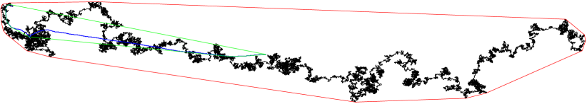
The process , , is the centre of mass process associated with the random walk. Under assumption ((M): ), satisfies law of large numbers and central limit theorem asymptotics of the same order as , but, locally, moves much more slowly, which leads, for example, to the interesting fact that is compact-set transient when and ; see [10, 19, 18] for these and other properties. Here we consider its convex hull, defined by . By convexity, and so ; see Figure 1 for a simulation picture. If , , and , another application of the ideas of the present paper (see Theorem 3.4 below) shows that
| (1.4) |
where . It would be interesting to evaluate ; presently, we do not have a solution to the variational problem that characterizes , which seems to require some new ideas. In Proposition A.1 in Appendix A below, we show that ; for comparison with (1.2), note that .
Open problem.
Compute the constant in (1.4).
Our main iterated-logarithm result for includes not only (1.2), but results for all dimensions and all intrinsic volumes, and permits general . In most cases, however, unlike (1.2), we do not have an explicit value for the constant. Our approach (like Khoshnevisan’s) is founded on Strassen’s functional law of the iterated logarithm, modified appropriately to apply to walks with non-zero drift; in our setting, as in Khoshnevisan’s, limiting constants can often be characterized by variational problems, but in only a limited number of instances is the solution known. We introduce some more notation in order to state our main results.
Let denote a non-empty, compact, convex subset of , and its volume (-dimensional Lebesgue measure). If , , denotes the parallel body , then the Steiner formula of integral geometry [33, §4.1] says that
| (1.5) |
where is the -dimensional volume of the unit-radius Euclidean ball in . The quantities on the right-hand side of (1.5) are the intrinsic volumes of . In particular, , and the intrinsic volumes and are proportional to the mean width and (Minkowski) surface area , respectively: specifically, and , see e.g. [11, p. 104].
Consider the random variables , . The strong law for the convex hull in the case with drift (see Theorem 3.3.3 of [24]) says that if , then , a.s., where the convergence is in the metric space of non-empty compact, convex sets. The limit set is a line segment of length . As can be seen from the Steiner formula (1.5) (see also [6, p. 7]), for , the only non-trivial intrinsic volume of is ; one has for . This means that from the strong law one obtains the rather limited information that, a.s.,
| (1.6) |
where we have used the fact that is continuous and homogeneous of order (see Definition 2.3 below).
Theorem 1.1, our first main result, gives more precise information about the a.s. large- behaviour of the intrinsic volumes . Recall that the random walk is genuinely -dimensional if is not supported by any -dimensional subspace [37, p. 72]; under assumption ((M): ), this is equivalent to being (strictly) positive definite. Throughout the paper, we write .
Theorem 1.1.
Suppose that ((M): ) holds with . Let . Then there exists a constant , depending on , , and the law of , such that
| (1.7) |
Moreover, if is genuinely -dimensional, then .
When , the result (1.7) is already contained in (1.6), so the main interest in Theorem 1.1 is when (see also Remarks 1.3 below). We do not have, in general, a formula for the constants appearing in (1.7), but we do have a Strassen-type variational characterization in the case (the volume), in which case depends on only via and , through an isoperimetric problem reminiscent of the classical Dido problem, for which we can provide an explicit solution when . To present these results (Theorem 1.2 below) we need some additional notation.
The symmetric, non-negative definite covariance matrix defines a linear transformation of . If and (non-zero drift), we denote by the matrix of the linear transformation on induced by the action of on the orthogonal complement of the linear subspace generated by . In other words, if is expressed in an orthonormal basis of that includes as a basis vector, the -dimensional reduced covariance matrix is obtained by deleting the row/column corresponding to ; note that since , in the definition of one could replace by and get the same reduced matrix.
For , , define the space–time convex hull of by
| (1.8) |
Let , , denote the set of , with , whose Cartesian components are absolutely continuous, and satisfy .
Theorem 1.2.
Remarks 1.3.
-
(a)
If is genuinely -dimensional, then .
- (b)
- (c)
- (d)
Here we give a brief overview of the remaining part of the article. We obtain our LIL for intrinsic volumes, Theorem 1.1, from a functional law of the iterated logarithm for convex hulls of random walks with drift, in the vein of (and proved using) Strassen’s celebrated functional law of the iterated logarithm [40]. Our result is a companion to a LIL of Khoshnevisan [14] which applies to functionals of convex hulls of zero-drift random walks. In Section 2 we review the Strassen-type theorem that we will need (Theorem 2.2) and present a small extension of Khoshnevisan’s result (Theorem 2.4) to permit general . In Section 3 we present analogues of the Strassen and Khoshnevisan results in the case of non-zero drift, and give the proof of Theorem 1.2, up to the evaluation of the constant . The classical normalization in the LIL is the Khinchin scaling function ; since our walks have non-zero drift, we instead scale the drift direction linearly (order ), and the other coordinates with the Khinchin scaling: see (3.1) below. The proof of Theorem 1.1 needs some additional work to overcome the fact that most intrinsic volumes do not scale simply under our non-isotropic scaling transformation: the main additional ingredient is a zero–one law for functionals of convex hulls of random walks with non-zero drift. This zero–one law is the subject of Section 4, which also contains the proof of Theorem 1.1. Section 5 is devoted to the evaluation of the constant from Theorem 1.2, by solving a planar isoperimetric problem similar to the classical Dido problem.
2. Iterated-logarithm laws of Strassen and Khoshnevisan
In this section we review Strassen’s functional LIL, first in the case of -dimensional Brownian motion (Theorem 2.1) and then for zero-drift random walk (Theorem 2.2). We then present (a slight generalization of) a theorem of Khoshnevisan of functionals of convex hulls of random walks (Theorem 2.4). As a first application, we deduce a shape theorem extending one from [25] (Corollary 2.5). It is worth pointing out that the LILs of Strassen and Khoshnevisan were both partially anticipated by a spectacular 1955 paper of Lévy [17].
Let denote the set of continuous , and let denote the subset of those for which . Endowed with the uniform (supremum) metric defined by , is a complete metric space. In components, write , so . If is absolutely continuous, then its derivative exists a.e. If all components of are absolutely continuous, we say that is absolutely continuous; then the (componentwise) derivative exists a.e.
For , set
which defines the norm . Let denote the set of absolutely continuous with . Then is a Hilbert space (the Cameron–Martin space for the Wiener measure [30, p. 339]) with inner product , and norm
| (2.1) |
The unit ball
| (2.2) |
is compact; see [30, §VIII.2]. Let be a standard -dimensional Brownian motion. The Khinchin scaling function for the classical LIL is
| (2.3) |
For each , set
Strassen’s theorem for -dimensional Brownian motion (cf. [40]) states the following.
Theorem 2.1 (Strassen’s LIL for Brownian motion).
Let . A.s., the sequence in is relatively compact, and its set of limit points is as defined at (2.2).
In other words, Theorem 2.1 states that, a.s., (a) every subsequence of contains a further subsequence that converges, its limit being some , and (b) for every , there is a subsequence of that converges to . For instructive proofs of Theorem 2.1, see [31, pp. 225–230] (for ) or [30, pp. 346–348], [7, pp. 21–24] (for general ).
To state the random-walk version of Strassen’s LIL, for , define linear interpolation of the random walk trajectory, parametrized from time to , by
| (2.4) |
Then for every . Note also that , since the convex hull of is determined only by , (linear interpolation does not affect the convex hull).
The symmetric, non-negative definite matrix defined in ((M): ) has a unique symmetric, non-negative definite square-root , such that . The matrix acts as a linear transformation of via , , and, for , the function is given by , . If ((M): ) holds with , then Donsker’s theorem [41, p. 393] says that converges weakly to as . Strassen’s theorem for -dimensional random walk (cf. [40]) is as follows.
Theorem 2.2 (Strassen’s LIL for random walk).
Let . Suppose that ((M): ) holds with . A.s., the sequence in is relatively compact, and its set of limit points is .
The usual proof of the case of Theorem 2.2 goes by Skorokhod embedding and using the Brownian result, Theorem 2.1 (cf. [39, §3.5]). For , one substitutes a more sophisticated strong approximation argument, such as [29] or [8, Thm. 2]; Theorem 2.2 is also a consequence of more general results on Hilbert or Banach spaces [16, Ch. 8].
Define the Euclidean distance between points by , and between a point and a set by . Let denote the set of compact subsets of containing , endowed with the Hausdorff metric defined by . By we denote the set of all that are convex. If , then the trajectory (interval image) is in , and is in (cf. [11, p. 44]). The following terminology is standard.
Definition 2.3 (Homogeneous function).
The function is homogeneous of order if for all and all scalar .
The following geometrical consequence of Theorem 2.2 is essentially Proposition 3.2 of Khoshnevisan [14], although we relax the assumptions in [14] to permit arbitrary ; see also [15, pp. 465–6].
Theorem 2.4 (Khoshnevisan).
Proof.
This theorem applies to an intrinsic volume, because the intrinsic volume function is continuous and homogeneous of order (see e.g. Theorem 6.13 of [11, p. 105]).
Khoshnevisan also formulated a version of Theorem 2.4 for Brownian motion (which is deduced from Theorem 2.1 in the same way as Theorem 2.4 is obtained from Theorem 2.2); important antecedent results in that setting are due to Lévy [17] and Evans [9, §1.3].
A further consequence (of either Theorem 2.2 or Theorem 2.4) is the following extension of Theorem 1.5 of [25], which dealt with the case , to general dimensions; the proof of [25] also readily extends to prove Corollary 2.5, so we only indicate the argument here to demonstrate how the Strassen-type results can be applied. Write for the diameter of .
Corollary 2.5 (Shape theorem).
Suppose that ((M): ) holds with , and that is (strictly) positive definite. Then for every with ,
Proof.
Since is full rank, the random walk is genuinely -dimensional, and , a.s. (by, e.g. Corollary 9.4 of [20]). For , define if , and otherwise. Then is continuous outside the set (cf. Lemma 3.6 of [25]) and hence Theorem 2.2 implies, similarly to in the proof of Theorem 2.4, that, a.s.,
Any can be arbitrarily well-approximated in Hausdorff distance by a polytope for some finite set of points (see Theorem 1.8.16 of [33]). Given , set for , and define by for , with linear interpolation; in words, is a polygonal path, parametrized by arc length, that visits in sequence. Then for a.e. , so has , and approximates with an error that can be made arbitrarily small. ∎
3. A Strassen-type theorem for the case with drift
In this section we present analogues of the LIL results of Section 2 for the case of a non-zero drift; essentially these results are obtained by combining the strong law of large numbers for the drift with Strassen’s law for the coordinates orthogonal to the drift. To motivate the random-walk result, we first consider the case of Brownian motion with drift in , . Suppose that is a Brownian motion with drift and infinitesimal covariance matrix , so that for .
Without loss of generality, we suppose coordinates are chosen so that the standard orthonormal basis of , , has . Write . For , we have , and so . Let denote the matrix obtained from by omitting the first row and column, i.e.,
which is the (symmetric, non-negative definite) infinitesimal covariance matrix of . Note that is the first principal minor of .
For , define , acting on , by
| (3.1) |
Let denote the function , and set
Observe that if , then (since entries of are uniformly bounded) too; since , it follows that whenever . In particular, . To enable us to include the (somewhat trivial) case in our statements, we also set .
Theorem 3.1.
Suppose that . A.s., the sequence in is relatively compact, and its set of limit points is .
Proof.
Here is the random-walk formulation. Recall the definition of from (2.4).
Theorem 3.2.
Suppose that ((M): ) holds with . A.s., the sequence in is relatively compact, and its set of limit points is . In particular, if is continuous, then , a.s.
Proof.
As a corollary, we obtain an analogue of Khoshnevisan’s theorem (Theorem 2.4) in the case with drift.
Corollary 3.3.
Suppose that ((M): ) holds with . Let be continuous. Then
As another application of Theorem 3.2, we give a LIL for the volume of the convex hull of the centre of mass process defined at (1.3), which includes the case stated at (1.4) above. Define for all by
One verifies that is indeed in , since .
Theorem 3.4 (LIL for the convex hull of the centre of mass).
Suppose that ((M): ) holds with . Then
where the constants are given via the variational formula
| (3.2) |
We defer the proof of Theorem 3.4 to Section A, since the proof runs along similar lines to parts of the proofs of our main results. We end this section with the proofs of our LIL for , Theorem 1.2.
Proof of Theorem 1.2..
By the scaling property of volumes, for ,
Then, by Corollary 3.3 with , we obtain, a.s.,
Now has for some , and, by scaling, if ,
where is defined at (1.8). Thus we deduce (1.11) and characterize the constant via (1.10). This completes the proof of part (i) of Theorem 1.2. For part (ii) of the theorem, we simply note from comparison of the strong law of large numbers in (1.6) with (1.7) in the case , we identify that . ∎
The proof of Theorem 1.1 needs more work, because for the functional does not behave so nicely under the scaling operation . The idea is to use the Strassen-type result Theorem 3.2 to obtain upper and lower bounds of matching order, and then conclude using a zero–one law. The next section presents this zero–one law (Theorem 4.4), which is of some independent interest, and then gives the proof of Theorem 1.1.
4. A zero–one law for walks with drift
Define . The event , that the convex hull asymptotically fills out all of space, has probability or as a consequence of the Hewitt–Savage zero–one law (see [20, p. 335]). Theorem 3.1 of [25, p. 7] provides a zero–one law for tail events associated with in the case where ; this follows from a Hewitt–Savage argument based on the fact that for every the initial trajectory is eventually enclosed in for all large enough, with probability 1. In the case with , one has either if (Corollary 9.4 in [20]), or if (Proposition 4.2 and Theorem 9.2 in [20]). In particular, in the case where , the zero–one law of [25] does not apply; see [20, §9] for some further remarks.
The purpose of this section is to provide a zero–one law that can be applied when . In this case, one cannot hope for a zero–one law that applies to all tail events of the type studied in [25] (see Remark 4.5 below), but we give a result that applies to a large class of functionals.
Write for the symmetric difference of sets and . Let denote the closed -dimensional Euclidean ball of radius centred at the origin. Our zero–one law will be stated for functionals acting on convex, compact sets containing the origin, satisfying the following property.
Definition 4.1.
We say is macroscopic if for every and there exists such that
| (4.1) |
Remark 4.2.
Note that if and , then ; hence one can formulate (4.1) equivalently with the condition rather than .
The macroscopic property in Definition 4.1 lends itself to our present application (see Proposition 4.6 for an explanation), but is also general enough to include the intrinsic volumes that are our main interest here, as well as a wide range of other examples, as we indicate in the next remark.
Remark 4.3.
Let (i.e., acting upon compact but not necessarily convex sets). Then is monotone if for every with , it holds that , and is subadditive if for every , . Take (i.e., convex) with . Clearly , while and so (since is convex) . Hence , which expresses the convex compact set as the union of two convex compact sets (‘’ denotes closure). Then, if is monotone and subadditive,
| (4.2) |
The similar argument with interchanged shows that if is both monotone and subadditive, then it satisfies the smoothness property
| (4.3) |
If (4.3) holds, then
which implies that is macroscopic (cf. Remark 4.2). Moreover, observe that in the inequality (4.2) the monotonicity and subadditivity of is required only on convex sets; in particular, it suffices that be a monotone valuation (cf. [11, p. 110] or [33, p. 172]). Some particular examples are as follows.
-
•
Intrinsic volumes are monotone valuations, hence macroscopic on .
-
•
Other monotone valuations include the rotation volumes and rigid motion volumes examined recently in [22].
-
•
The diameter function is monotone and subadditive on (for the latter, recall that on every set contains ), hence macroscopic on .
-
•
If is any transient random walk on , the associated capacity is given by , and is monotone and subadditive (see e.g. [37, §25]), hence macroscopic.
-
•
Fix and , and consider the function which counts the number of faces of whose length exceeds . Then the function on is neither monotone nor subadditive. We believe is nevertheless macroscopic, but we do not investigate this further here.
This list of examples shows that the class of macroscopic functionals contains functions quite different in nature from intrinsic volumes.
Here is the formulation of our zero–one law; we emphasize that we do not assume that .
Theorem 4.4 (Zero–one law).
Let . Suppose that and , and that is macroscopic (see Definition 4.1). Suppose also that
| (4.4) |
Then satisfies a zero–one law in the sense that for every sequence ,
| (4.5) |
Remark 4.5.
The condition (4.4) cannot be removed, in general. To see this, suppose that and , and consider the functional . Then is monotone and subadditive, hence macroscopic (see Remark 4.3). However, the random variables satisfy , a.s., which is just where is a one-dimensional random walk with strictly positive drift. As long as is non-degenerate, therefore has a non-trivial distribution, so (4.5) is violated (for , constant), and (4.4) fails. Note that the event is also a tail event for in the sense of [25, p. 7].
For a -dimensional real matrix , the matrix (operator) norm induced by the Euclidean norm is . We need a short calculation. For any absolutely continuous and any non-negative definite, -dimensional matrix , we have, adapting [14, p. 387],
and hence, by the triangle and Jensen inequalities,
| (4.6) |
Now we can complete the proof of our LIL for intrinsic volumes, Theorem 1.1.
Proof of Theorem 1.1..
Let . It suffices to suppose that is genuinely -dimensional (for if not, work instead in for ); hence . We will prove that there exist constants (where depend only on ) for which
| (4.7) |
Without loss of generality, choose the basis of so that is the first coordinate vector. For , define the rectangle . We will apply Theorem 3.2, which says that in is relatively compact, and its set of limit points is . Consider with (so that ). Then (4.6) applied to and with shows that is bounded by a finite constant. This means that there exists such that for every . Since is the set of limit points for , it follows that for every there exists a (random, a.s.-finite) such that for all , say. Hence we conclude that, a.s.,
| (4.8) |
On the other hand, it is not hard to see that, provided , there exist , and some for which . Thus, from Theorem 3.2, for every and we have that, a.s.,
| (4.9) |
Finally, the claim (4.7) follows from (4.8) and (4.9) together with the fact that
| (4.10) |
where is the th elementary symmetric polynomial in arguments; one can find (4.10) as Proposition 5.5 in [21]. This completes the proof of (4.7).
A consequence of (4.7) is that , a.s. By the zero–one law (Theorem 4.4) and the fact that the intrinsic volume functional is macroscopic (see Remark 4.3), we obtain that there is a constant for which
| (4.11) |
Then (4.11) combined with (4.7) shows that (recalling that we have assumed that is genuinely -dimensional). This completes the proof of (1.7). ∎
The rest of this section is devoted to the proof of Theorem 4.4. For , let denote the set of all such that is a permutation on and for all . Then the random walk (for ) defined by and , , takes the same increments as , but with a permutation among the first ; note that for all . Let .
For , define
| (4.12) |
and also define
| (4.13) |
Define , , analogously to (4.12)–(4.13) in terms of . Then, for every and all , it holds that for all .
The next proposition shows that for every , every permutation of changes the convex hull only within a finite region (with a random radius that depends on but not on ). Indeed, it follows from (4.15) below that
| (4.14) |
In particular, this means that macroscopic functionals are asymptotically approximately invariant under . This property is the key to our proof of Theorem 4.4. Theorem 6.2.2 of McRedmond [24] established a result along somewhat similar lines for the space-time convex hull of a one-dimensional random walk.
Proposition 4.6.
Let . Suppose that and . A.s., it holds for every that there exists for which
| (4.15) |
A crucial geometrical ingredient in the proof of Proposition 4.6 is provided by the next lemma, which says that eventually contains cylinders with axis in the direction of arbitrary radius and height. Define the cylinder . Denote for the sphere (a copy of ) orthogonal to .
Lemma 4.7.
Let . Suppose that and . Fix and . Then, a.s., there exists such that, for all but finitely many , .
Proof.
For , define to be the projection of onto the -dimensional subspace orthogonal to , and then set for . Here is a random walk on with mean drift in . Corollary 9.4 in [20] implies that satisfies for all .
Fix and . Then there exists an a.s.-finite (a stopping time) such that for all . Then set (so is a.s. finite). Since, by the strong law of large numbers, , a.s., there exists an a.s.-finite such that for all . There also exists an a.s.-finite such that . Furthermore, there exists an a.s.-finite such that for all . Therefore, is contained in the interior of , and so .
Proof of Proposition 4.6..
Fix (which we suppress in some of the subsequent notation). For , and , define
where is given by (4.13). Furthermore, for define
A consequence of Lemma 4.7 is that
| (4.18) |
Since, for fixed , is a non-decreasing sequence (in ) of compact sets, if , there is a (random but a.s. finite) time such that, for every , the convex hull contains , a sphere in the -dimensional hyperplane orthogonal to at distance from the origin in the direction. In particular, for all and all .
Set . Consider the (a.s.-finite) and associated time with the property described in the preceding paragraph. Then contains the sphere for every . Moreover, the random variables and are invariant under permutations of (since is invariant, and is defined in terms of ). Hence contains the sphere for every and every .
For , let , which is the relative boundary of in the hyperplane orthogonal to at distance . For every , the points are contained in the cylinder . Hence the minimal angle, over all , between and () is at least
Every has , and so the strong law of large numbers says that, as , , a.s. This holds a.s. simultaneously for every is a countable dense subset of , and hence , a.s., as . On the other hand, a.s., . Thus
Consequently, there exists a random time such that stays in a cone with vertex at some () and angular span , say, for all .
It follows that, for every and every , no can be included in any face of which also includes some member of . Let denote those faces of which include at least one of , and denote those faces of which use none of , and set . Since faces in can include only , every point of lies in , and the points can only appear as vertices in (and in no other faces of ). This means that is invariant under . Moreover, the vertices of faces in are necessarily from , which are included in . Hence for every . This completes the proof of (4.15). ∎
Proof of Theorem 4.4.
Since , the symmetric difference . Proposition 4.6 then shows that, for every , a.s., there exists such that, for every , . Suppose that is macroscopic. Then, taking and in (4.1), we see that for every there exists (depending on ) such that
By (4.4), it thus follows that, for every , a.s.,
Since was arbitrary, we conclude that
But is in the -permutable -algebra. Thus is also in the -permutable -algebra (extended, as usual, up to a.s.-equivalence). Since was arbitrary, it follows that is a.s. constant in , by the Hewitt–Savage zero–one law (see [4, pp. 232–238] for details, including the definition of the extended permutable -algebra). ∎
5. Evaluating the constant in the planar case
5.1. Solution to the isoperimetric problem
In this section we work with , which means our variational problem concerns functions , i.e. (see §2) that are absolutely continuous, have , and satisfy . We will write for simplicity; it is, however, helpful to generalize the domain of our functions from to .
For , let denote the set of that are absolutely continuous, have , and satisfy ; note that . Given , denote by and the least concave majorant and greatest convex minorant of over , so that the continuous functions and are such that for all , , , is concave, is convex, and the difference is minimal. It is easy to see that
| (5.1) |
For and Borel , define functionals
| (5.2) | ||||
| (5.3) | ||||
| (5.4) |
Note that we do not include in the notation the dependence on the upper endpoint of the domain of . If is an interval, we write for simplicity; similarly for and . When , as defined at (2.1), and for all . Also, by Cauchy–Schwarz, the arc length functional satisfies
| (5.5) |
and so (the supremum being attained by ).
Here is the main result of this section.
Theorem 5.1.
Let . The unique that maximizes subject to is given by
| (5.6) |
which has and .
The following subsections lay out the proof of Theorem 5.1. Before doing so, we make some remarks on the relation of Theorem 5.1 to some of the classical problems of isoperimetry. Dido’s Problem is to find the rectifiable planar curve of a given length to maximize the area of the corresponding convex hull. In terms of the area and arc-length functions and defined at (5.2) and (5.3), the solution to the Dido problem reduces to the statement (see e.g. Theorem 1.1 of [42]) that
with equality attained by the semicircle described by . The function has and ; the semicircle whose curved boundary has the same arc length has area .
The fact that the optimal curve in Dido’s problem is a semicircle had been known since antiquity, although proofs that are fully rigorous by modern standards are more recent: see e.g. [42, 28, 26, 34] for precise statements and proofs of this result and higher-dimensional analogues, and e.g. [46] for a survey of neighbouring results in isoperimetric problems.
5.2. Preliminaries
We will show that it suffices to prove Theorem 5.1 for the case . To do so, we first establish some basic results on how the functionals and behave under affine transformations. Given , define the function by
Lemma 5.2.
Let . If , then
On the other hand, if , then
Proof.
Suppose that . The affine transformation preserves convexity. Thus if and are the concave majorant and convex minorant, respectively, and . Hence
Moreover, since ,
The other case is similar. ∎
The next lemma shows that it suffices to consider the case of subject to .
Lemma 5.3.
Suppose that there exists a unique that maximizes subject to ; denote this by . Then for any there exists a unique that maximizes subject to , and this is given by
| (5.7) |
Moreover,
| (5.8) |
Proof.
Suppose existence of the optimal is given, as described, with . Then defined by has and (as follows from the case of Lemma 5.2). This would contradict optimality of unless ; hence .
5.3. Reduction to non-negative bridges
Lemma 5.3 shows that to prove Theorem 5.1, it suffices to suppose that and . In this subsection we further reduce the class of functions that we need to consider; the next step is to show that it suffices to work with bridges. Let (the set of bridges) and (non-negative bridges). Observe that if then and , so . Moreover, if then and so
| (5.9) |
with equality if and only if is concave.
For , define by
| (5.10) |
Lemma 5.4.
Suppose that . Then (i) ; (ii) ; and (iii) , with equality if and only if .
Proof.
The function defined by is concave, since is concave, and satisfies for all . Moreover, if is any concave majorant of , then the function is a concave majorant of ; hence must be the least concave majorant of . Similarly, is the greatest convex minorant of . Thus , as claimed. Now, since , we have , and hence
with equality if and only if . In particular, , and by (5.10), so in fact . ∎
Subsequent reductions will be based on some surgeries applied to our functions. To describe them, we introduce notation associated with the faces of the convex hull.
Suppose that is not the constant (zero) function. Consider the concave majorant of . Then can be partitioned as , where are the indices of extreme points of [11, p. 75], and are indices of points in the interior of faces of : that is, if and only if there is a unique supporting half-plane at whose boundary , , intersects for in an open interval containing .
Similarly, we have , where and correspond to extreme points and faces of . Write . Note that . Moreover, every has (if ) or (if ), and, since is not linear, the observation (5.1) shows that , and so we can speak of as being the set of extreme points, without the possibility of duplications. Put differently, every must belong to at least one of , i.e., .
The set is a union of disjoint (maximal) open intervals in , each interval corresponding to the horizontal span of a face of . For every there are at most finitely many such intervals of length more than , so is a union of at most countably many disjoint open intervals. Enumerate the intervals of from left to right by , . Similarly, enumerate the intervals of by , . By construction for all . For reference, we summarize the preceding discussion in the following lemma.
Lemma 5.5.
Suppose is not the zero function. There exist two partitions of , , with the following properties.
-
•
Each set is the union of pairwise disjoint intervals: , where , it holds that , and the index set is finite or countably infinite.
-
•
We have .
-
•
For all , , and, for all , .
The following result shows that it suffices to consider non-negative bridges.
Proposition 5.6.
For every , there exists for which (i) ; and (ii) .
The proof of the Proposition 5.6 uses a kind of symmetrization, which is a common idea in isoperimetric problems (see e.g. the recent work [3, 36]).
Definition 5.7.
See Figure 2 for an illustration: is constructed by a sequence of reflections (more accurately, each is a time-reversal and change of sign) across each straight-line face of the concave majorant of ; similarly, is derived from the convex minorant. The proof of Proposition 5.6 amounts to establishing that the in the claim in therein can be chosen to be one of or defined at Definition 5.7. The following series of properties will establish this.
Lemma 5.8.
Suppose , and consider the functions and defined at Definition 5.7. Then (i) with for all ; (ii) with for all ; (iii) ; (iv)
| (5.11) |
and (v) .
Proof.
Consider the function . If , then . Otherwise, for some . On this interval, is the line segment (face) given by
and for all . Hence, for ,
| (5.12) |
An analogous argument gives
| (5.13) |
Since is absolutely continuous, the function is also absolutely continuous. Hence the derivative exists for a.e. . Since coincides with on , we have for a.e. . On the other hand, for , we have for a.e. , and so
the last equality obtained using the substitution . Hence . A similar argument shows that , verifying (iii). Moreover, the fact that together with the relation (5.3) implies (i), and, similarly, from (5.13) we get (ii).
Proof of Proposition 5.6..
Lemma 5.8 shows that we may take to be whichever one of or achieves the maximum in . ∎
Our final reduction is simple: we can replace a non-negative bridge by its concave majorant.
Lemma 5.9.
Suppose that . Then has and .
Proof.
Suppose that . It follows from Lemma 5.5 that we can recover from by replacing over every interval by the straight line segment from to . This preserves the value of the area enclosed by the concave majorant, but can not increase the value of , since for and , we have , and
which is minimized when is the straight line. ∎
5.4. Identifying the optimal function
The reductions in Section 5.3 show that we can reduce the problem to that of non-negative bridges that are their own least concave majorant. The final step is the following.
Lemma 5.10.
Suppose that . Then
with equality if and only if .
Remark 5.11.
Lemma 5.10 is closely related to results of Schmidt [32], although Schmidt’s main results are concerned with functions with changes of sign; we give a short self-contained proof here, and indicate where a key step in our argument can be substituted by a secondary result from [32]. See also [27] (particularly Chapters IV & XV) for a host of adjacent results.
Proof of Lemma 5.10..
Suppose that . Observe that
where the last inequality is Cauchy–Schwarz, and the condition for equality is that and are linearly dependent. Since , that is
| (5.14) |
with equality in (5.14) if and only if for all and some . (The inequality (5.14) is the , , case of (20) in [32, p. 306].) The same argument with shows that
| (5.15) |
with equality in (5.15) if and only if for all and some . From (5.14) and (5.15) we obtain
| (5.16) |
Suppose that . Now, by Jensen’s inequality, , with equality if and only if , so we have from (5.4) that
with equality if and only if both equality holds in the Cauchy–Schwarz and Jensen inequalities, i.e., , for , and for . Thus in the case of equality, we must have , and , which is when . ∎
We can now complete the proof of Theorem 5.1.
Proof of Theorem 5.1..
Lemma 5.4, Proposition 5.6, and Lemma 5.9 show that to every one can associate that is non-negative and concave, and for which but . Hence the optimal is attained by some that is non-negative and concave. For such an , we have and , so is simply the integral of ; Lemma 5.10 then shows that is optimal. ∎
Appendix A Proof of the LIL for the centre of mass
This section deals with the centre of mass process defined by (1.3), and its associated convex hull . In particular, we prove our LIL in this context, Theorem 3.4, which in the planar case is the statement (1.4), and Proposition A.1, which gives a lower bound on the constant in (1.4).
Proof of Theorem 3.4..
Observe that is a (Lipschitz) continuous functional since, for all ,
so . Hence the functional is continuous from . Recall the definition of the interpolated trajectory from (2.4). Theorem 3.2 implies that the sequence in is relatively compact, and its set of limit points is . Every is of the form for , and then . We can now argue similarly to in the proof of Theorem 1.2 above to get
| (A.1) |
with as defined at (3.2). The LIL at (A.1) does not yet yield the LIL in Theorem 3.4, because, unlike the analogous step in the proof of Theorem 1.2, there is a discrepancy between (for the interpolated path ) and . To quantify the error, write for and ,
We claim that
| (A.2) |
The bound (A.2) will allow us to bound the difference between and using the Steiner formula (1.5); to do so, we need bounds on the lower intrinsic volumes. At this point we can apply Theorem 3.2, and argue as in the proof of Theorem 1.1 that, similarly to (4.7), for each , there is a constant for which
| (A.3) |
(Note that in (A.3) we are not claiming that the is a.s. constant, and we have not claimed that the zero–one law in Theorem 4.4 applies.) From (A.2), (A.3), and monotonicity of intrinsic volumes, we obtain from the Steiner formula (1.5) that, for every ,
| (A.4) |
Then (A.4) together with (A.1) yields the LIL in Theorem 3.4.
It remains to verify the claim (A.2). For and ,
For simplicity of notation, write and , so that and , and . Then
where, for any , by (2.4),
It follows that
Hence, for ,
Thus we obtain, by the triangle inequality,
which is a.s. finite, since the strong law implies that and (see e.g. Proposition 1.1 of [19]). This verifies (A.2) and hence completes the proof. ∎
In the remainder of this section, we establish the following bound on the constant from (1.4).
Proposition A.1.
It holds that .
Proof.
The case of Theorem 3.4 says that, if ,
where, by (3.2), . Comparison with (1.4) shows that
| (A.5) |
The proof of Proposition A.1 goes by exhibiting an for which . Define the one-parameter family by
| (A.6) |
Then the choice yields the stated bound (we explain below the origin of this choice of parametric family, and the numerical choice of ). Indeed, the concave majorant of for with this choice of coincides with over an interval and then follows the straight line to ; numerical calculation gives and then , as claimed. ∎
We end this section with an heuristic explanation for how we went about looking for the exhibited in the proof of Proposition A.1, as this may prove useful for readers who seek to improve our bound. First note that some calculus yields
While it is not at all clear that the reductions for the analogous problem presented in Section 5.3 are applicable in this case, following the reasoning of Lemma 5.10 suggests trying to choose to
| (A.7) |
The which solves (A.7) is of the form , and the two constraints in (A.7) fix and , to give the one-parameter family defined at (A.6). The optimal for (A.7) has , which gives . However, the that results from is non-concave, so in fact . This means that (A.7) is not the correct optimization problem to evaluate ; but restricting ourselves to functions of the form given at (A.6), we may nevertheless try to maximize . Rather than , numerical experimentation shows that a better choice is , as we used in the proof of Proposition A.1.
Appendix B Some extensions of Khoshnevisan’s examples for the zero-drift case
If for a symmetric, nonnegative-definite -dimensional matrix with symmetric square-root , then is univariate normal with mean and variance . Since is symmetric, its largest eigenvalue is given by
| (B.1) |
Then is the largest eigenvalue of ; let denote a unit-length eigenvector of corresponding to .
Example B.1 (Diameter).
Suppose that and ((M): ) holds with . Then
| (B.2) |
To prove this, observe that, from (4.6) applied to with ,
| (B.3) |
by (B.1). On the other hand,
Take , so and , to see that
| (B.4) |
Combining (B.3) and (B.4), we obtain (B.2) by an application of Theorem 2.4 with , noting that the diameter functional is homogeneous of order . This extends Khoshnevisan’s Example 4.1 [14, pp. 387–388], which had . ∎
Remark B.2.
The result (B.2) may be compared with
| (B.5) |
as can be obtained either from Strassen’s theorem (Theorem 2.2), or directly from the one-dimensional Hartman–Wintner LIL [4, p. 382]. Indeed, the one-dimensional random walk satisfies
where . This holds simultaneously for all in a countable dense subset of , which is enough to conclude (B.5), since and .
Example B.3 (Volume).
Suppose that and ((M): ) holds with . Then, there exists a constant such that
| (B.6) |
where . Khoshnevisan [14, p. 389] established (B.6) in the case and proved that . The case of general follows from Theorem 2.4 with (a functional that is homogeneous of order ) in the same way as described in [14], accounting for the linear transformation . ∎
Acknowledgements
Much early impetus for this work was provided by stimulating discussions with James McRedmond and Vlad Vysotsky; in particular, James identified the quadratic function as a likely candidate for the solution to the isoperimetric problem in Theorem 5.1, and Vlad suggested a Strassen-type approach to shape theorems as in Corollary 2.5. The authors also express their thanks to the Institute of Mathematical Stochastics at TU Dresden, for hospitality in hosting a stimulating research visit in September 2022. This visit was supported by Alexander-von-Humboldt Foundation project No. HRV 1151902 HFST-E. The work of AW was supported by EPSRC grant EP/W00657X/1.
References
- [1] A. Akopyan and V. Vysotsky, Large deviations of convex hulls of planar random walks and Brownian motions. Ann. Henri Lebesgue 4 (2021) 1163–1201.
- [2] D. Bang, J. González Cázares, and A. Mijatović, Asymptotic shape of the concave majorant of a Lévy process. Ann. H. Lebesgue 5 (2022) 779–811.
- [3] G. Bianchi, R.J. Gardner, and P. Gronchi, Symmetrization in geometry. Adv. Math. 306 (2017) 51–88.
- [4] Y.S. Chow and H. Teicher, Probability Theory. 3rd ed., Springer, New York, 1997.
- [5] M. Cranston, P. Hsu, and P. March, Smoothness of the convex hull of planar Brownian motion. Ann. Probab. 17 (1989) 144–150.
- [6] W. Cygan, N. Sandrić, and S. Šebek, Convex hulls of stable random walks. Electron. J. Probab. 27 (2022), article no. 98, 30 pp.
- [7] J.-D. Deuschel and D.W. Stroock, Large Deviations. Academic Press, San Diego, 1989.
- [8] U. Einmahl, Strong invariance principles for partial sums of independent random vectors. Ann. Probab. 15 (1987) 1419–1440.
- [9] S.N. Evans, Local Properties of Markov Families and Stochastic Processes Indexed by a Totally Disconnected Field. Ph.D. Thesis, University of Cambridge, 1986.
- [10] K. Grill, On the average of a random walk. Statist. Probab. Letters 6 (1988) 357–361.
- [11] P.M. Gruber, Convex and Discrete Geometry. Springer, Berlin, 2007.
- [12] Z. Kabluchko, V. Vysotsky, and D. Zaporozhets, Convex hulls of random walks: Expected number of faces and face probabilities. Adv. Math. 320 (2017) 595–629.
- [13] J. Kampf, G. Last, and I. Molchanov, On the convex hull of symmetric stable processes. Proc. Amer. Math. Soc. 140 (2012) 2527–2535.
- [14] D. Khoshnevisan, Local asymptotic laws for the Brownian convex hull. Probab. Theory Relat. Fields 93 (1992) 377–392.
- [15] J. Kuelbs and M. Ledoux, On convex limit sets and Brownian motion. J. Theoretical Probab. 11 (1998) 461–492.
- [16] M. Ledoux and M. Talagrand, Probability in Banach Spaces: Isoperimetry and Processes. Classics in Mathematics, Springer, New York, 2011.
- [17] P. Lévy, Le caractère universel de la courbe du mouvement brownien et la loi du logarithme itéré. Rend. Circ. Mat. Palermo 4 (1955) 337–366.
- [18] C.H. Lo, J. McRedmond, and C. Wallace, Functional limit theorems for random walks. Preprint (2018) ArXiv: 1810.06275.
- [19] C.H. Lo and A.R. Wade, On the centre of mass of a random walk. Stochastic Process. Appl. 129 (2019) 4663–4686.
- [20] A. López Hernández and A.R. Wade, Angular asymptotics for random walks. A Lifetime of Excursions Through Random Walks and Lévy Processes: A Volume in Honour of Ron Doney’s 80th Birthday, pp. 315–342, Springer, 2021.
- [21] M. Lotz, M.B. McCoy, I. Nourdin, G. Peccati, and J.A. Tropp, Concentration of the intrinsic volumes of a convex body. Geometric Aspects of Functional Analysis. Vol. II, pp. 139–167, Springer, 2020.
- [22] M. Lotz and J.A. Tropp, Sharp phase transitions in Euclidean integral geometry. Preprint (2022) ArXiv: 2208.13919.
- [23] S.N. Majumdar, A. Comtet, and J. Randon-Furling, Random convex hulls and extreme value statistics. J. Stat. Phys. 138 (2010) 955–1009.
- [24] J.F.W. McRedmond, Convex Hulls of Random Walks. Ph.D. Thesis, Durham University, 2019. http://etheses.dur.ac.uk/13281/.
- [25] J. McRedmond and A.R. Wade, The convex hull of a planar random walk: perimeter, diameter, and shape. Electron. J. Probab. 23 (2018) paper no. 131, 24 pp.
- [26] Z.A. Melzak, The isoperimetric problem of the convex hull of a closed space curve. Proc. Amer. Math. Soc. 11 (1960) 265–274.
- [27] D.S. Mitrinović, J. Pečarić, and A.M. Fink, Inequalities Involving Functions and Their Integrals and Derivatives. Springer, Netherlands, 1991.
- [28] P.A.P. Moran, On a problem of S. Ulam. J. London Math. Soc. 21 (1946) 175–179.
- [29] W. Philipp, Almost sure invariance principles for sums of -valued random variables. Probability in Banach spaces, II, pp. 171–193, Lecture Notes in Math., 709, Springer, Berlin, 1979.
- [30] D. Revuz and M. Yor, Continuous Martingales and Brownian Motion. 3rd ed., Springer, Berlin, 2005.
- [31] R.L. Schilling, Brownian Motion. 3rd ed., De Gruyter, Berlin/Boston, 2021.
- [32] E. Schmidt, Über die Ungleichung, welche die Integrale über eine Potenz einer Funktion und über eine andere Potenz ihrer Ableitung verbindet. Math. Ann. 117 (1940) 301–326.
- [33] R. Schneider, Convex Bodies: The Brunn–Minkowski Theory. 2nd ed., Cambridge University Press, Cambridge, 2014.
- [34] I.J. Schoenberg, An isoperimetric inequality for closed curves convex in even-dimensional Euclidean spaces. Acta Math. 91 (1954) 143–164.
- [35] T.L. Snyder and J.M. Steele, Convex hulls of random walks. Proc. Amer. Math. Soc. 117 (1993) 1165–1173.
- [36] A.Yu. Solynin, Exercises on the theme of continuous symmetrization. Comput. Methods Funct. Theory 20 (2020) 465–509.
- [37] F. Spitzer, Principles of Random Walk. 2nd ed., Springer, New York, 1976.
- [38] F. Spitzer and H. Widom, The circumference of a convex polygon. Proc. Amer. Math. Soc. 12 (1961) 506–509.
- [39] W.F. Stout, Almost Sure Convergence. Academic Press, New York, 1974.
- [40] V. Strassen, An invariance principle for the law of the iterated logarithm. Z. Wahrschein. verw. Gebiete 3 (1964) 211–226.
- [41] D.W. Stroock, Probability Theory: An Analytic View. 2nd ed., Cambridge University Press, Cambridge, 2011.
- [42] P. Tilli, Isoperimetric inequalities for convex hulls and related questions. Trans. Amer. Math. Soc. 362 (2010) 4497–4509.
- [43] V. Vysotsky, The isoperimetric problem for convex hulls and the large deviations rate functionals of random walks. Preprint (2023) ArXiv: 2306.12359.
- [44] A.R. Wade and C. Xu, Convex hulls of planar random walks with drift. Proc. Amer. Math. Soc. 143 (2015) 433–445.
- [45] A.R. Wade and C. Xu, Convex hulls of random walks and their scaling limits. Stochastic Process. Appl. 125 (2015) 4300–4320.
- [46] V.A. Zalgaller, Extremal problems concerning the convex hull of a space curve. St. Petersburg Math J. 8 (1997) 369–379.