When Dialects Collide:
How Socioeconomic Mixing Affects Language Use

Abstract

The socioeconomic background of people and how they use standard forms of language are not independent, as demonstrated in various sociolinguistic studies. However, the extent to which these correlations may be influenced by the mixing of people from different socioeconomic classes remains relatively unexplored from a quantitative perspective. In this work we leverage geotagged tweets and transferable computational methods to map deviations from standard English on a large scale, in seven thousand administrative areas of England and Wales. We combine these data with high-resolution income maps to assign a proxy socioeconomic indicator to home-located users. Strikingly, across eight metropolitan areas we find a consistent pattern suggesting that the more different socioeconomic classes mix, the less interdependent the frequency of their departures from standard grammar and their income become. Further, we propose an agent-based model of linguistic variety adoption that sheds light on the mechanisms that produce the observations seen in the data.

Introduction

As a primary means of communication, language shapes social interactions, and in return it is shaped by society and its many aspects. Due to this circular relationship, one may naturally expect to see social differences between individuals reflected in the language they use. Culture, politics, education, or the economy: all of these spheres of society can be decisive in shaping language and its variety. In this work, we look in particular into the relationship between the use of standard language and socioeconomic status (SES). The standard variety of a language is defined by norms set by the language ideology of a society’s major institutions. As such, this variety may be promoted by these institutions in a number of ways. The use of this form in official communications, in mainstream media, or simply and most importantly, by teaching it in schools are all good examples for such influences  (?). And, as argued by Pierre Bourdieu  (?), all these influences confer a higher value to this particular linguistic variety in society, thus individuals who use it are attributed more linguistic capital. However, language is not only a commodity with each of its variety being attributed some market value. Indeed, individuals may also attribute a non-market value to a language variety  (?, ?), just as speakers of different languages may attribute more cultural value to a language  (?, ?): this is what is known as differing language attitudes  (?). Therefore, despite the higher market value of the standard form, some may use other varieties of their language  (?), as they have their own perception of what is the “normal” way of speaking  (?). As it turns out, it is not uncommon that some classes of the population, particularly those of relatively low SES, prefer to use a non-standard form. This has been shown by sociolinguists in the past, as they conducted field studies and analysed differences between socioeconomic classes, notably in matters of accent and phonology  (?, ?, ?, ?). As groups of lower SES can then be attributed less linguistic capital, their economic opportunities may also be affected. SES and this linguistic variation could thus be mutually sustaining: one inherits an SES along which comes a linguistic capital that contributes — among other things — to constrain individuals to their status of origin. Understanding the mechanisms that lead to this linguistic segregation is therefore of great importance. Although this phenomenon has long been known  (?), it has been observed on very limited scales, and, more importantly, no model explaining how it might emerge has been proposed. These are the two shortcomings we wish to address in this paper.

The PISA reports of the OECD  (?) consistently show in a quantified manner that students with lower socioeconomic background tend to have a lower reading proficiency. While these reports confirm there is an issue to tackle, they are not extensive enough. They do not test language production, and not the whole population but only a sample of students of a specific age. Alternative empirical works are thus needed to understand better the phenomenon. Data from social media have repeatedly proven useful to link SES and different social behaviours  (?). In particular, Twitter data were used in the past to study linguistic features and their variation, whether lexical  (?, ?, ?, ?, ?, ?), semantic  (?, ?), or in spelling  (?, ?, ?). These dimensions of variation have sometimes even been mapped geographically, leveraging the geotags that users may attach to their tweets. Having these features mapped geographically, it further enabled researchers to relate linguistic variation to some social variable characterising the populations of the areas under study. However, this data source has yet to unlock its full potential to explore the complex interplay between language variation and SES. A first step was taken in  (?), where the authors analyse a few markers of non-standard language in France and their socioeconomic dependencies. Here, we perform a two-fold approach, both empirical and theoretical, to investigate how Twitter users in England and Wales abide by the rules of the standard variety of English. Remarkably, we find that this is determined not only by SES but more crucially by the interaction strength between socioeconomic (SE) classes

Results

Spatial combination of linguistic and socioeconomic data

We leverage a database containing slightly more than $550$ million geotagged tweets posted from Great Britain by around $4.5$ million users between 2015 and 2021 (for more details about the dataset see Materials & Methods). These tweets were collected through the filtered stream endpoint of the Twitter application programming interface. First, from all collected tweets, we identify users who may be residents of England and Wales, following the methodology described in Materials & Methods. To assign an SES indicator to each user, we determine their area of residence from the geotags attached to their tweets, following the heuristics described in Materials & Methods. Our unit areas for the study are the $7201\text{\,}$ middle layer super output areas (MSOAs), which are areas created by the Office for National Statistics of the UK for the output of the census estimates. In the following, we will refer to them as cells to avoid using this abbreviation. Each cell hosts at least $5000\text{\,}$ and at most $15000\text{\,}$ inhabitants, with a typical population of $8000\text{\,}$. The average annual net income in these cells can be obtained from the census. This way, we couple Twitter users to a proxy indicator of their SES.

The second ingredient we need for our analysis is a measurement of people’s propensity to deviate from the rules that define standard English. The solution we picked to measure these deviations is to use LanguageTool, an open-source grammar, style, and spell checker. There are several advantages of using such a tool over a pre-defined set of rules, as in  (?). First, this tool covers a very wide spectrum of potential mistakes: it has more than $5500\text{\,}$ rules defined for the English language. These rules are split into 11 categories, among which are grammar mistakes, confused words or typos. In this work we focus on grammar mistakes, as we found them to be among the most common and the most characteristic of non-standard language (see LABEL:SItab:cats_global_stats of the Supplementary Material). Within that category, we provide the ten most common rules that were broken by Twitter users in LABEL:SItab:top_grammar_mistakes. Another important advantage of the tool is that it is implemented in $15$ languages. Our study could thus quite easily be replicated in other countries.

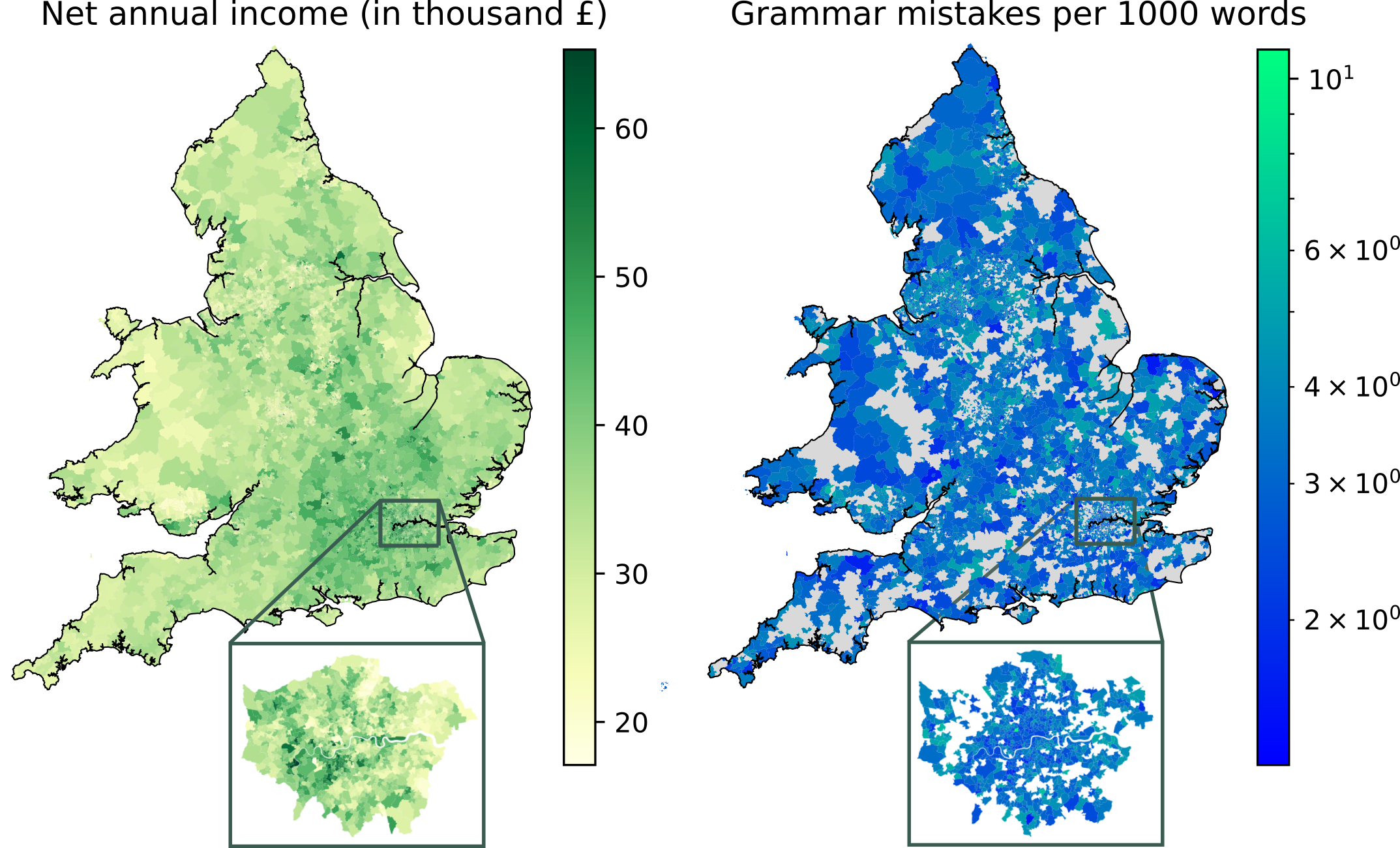
Figure 1: Side-by-side maps of our socioeconomic and linguistic variables. They present the average net annual income given by the census, and the average frequency of grammar mistakes that we measured from our Twitter dataset in the MSOAs of England and Wales. For the latter, we only colour cells with sufficient Twitter population, following the residence attribution detailed in Materials & Methods, and a logarithmic scale is used to better visualise geographical variations. As an example, for both maps we provide a zoom-in on London showing the variation of these two variables in the city.

After pre-processing the text of tweets and detecting them reliably as having been written in English, as explained in Materials & Methods, we therefore pass them through LanguageTool to compute the frequency at which users make grammar mistakes according to standard rules. From this raw frequency, we then compute the frequency of mistakes per word written by each user. As the activity of Twitter users was previously found to follow a log-normal distribution spanning almost four orders of magnitude  (?), we compute this frequency at the single user level, to be more representative of the general population, and not only of the few very active users. In any case, we remove inactive users and keep only ones who have written at least $100$ words. Then, at the cell level, we compute the average of the individual relative frequencies for all residents. To exclude cells with too little statistics, we only kept cells with at least $15$ residents left after applying the previous filter. This leaves us with $131402\text{\,}$ users spread across $4879\text{\,}$ MSOAs. In our study we concentrate on eight metropolitan areas around London, Manchester, Birmingham, Liverpool, Leeds, Bristol, Newcastle upon Tyne, and Sheffield. The precise definitions that we used for these metropolitan areas is given in LABEL:SItab:uk_metropolitan_areas. A population density map of Twitter users we obtained through this pipeline is shown in LABEL:SIfig:EW_twitter_pop for the whole country and the analysed metropolitan areas too. In the end, in every remaining MSOA, our analysis yields an estimate of the income of its residents, which serves as a proxy for their SES, and of the frequency at which they make grammar mistakes, which indicates how much they tend to deviate from a standard usage of English. These two features are mapped side-by-side in Fig. 1. The results from our data processing are summarised in LABEL:SItab:dataset_summary.

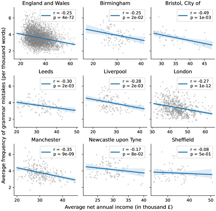
Figure 2: Correlation between frequency of grammar mistakes and net income. We show them for all MSOAs of England and Wales, and then of the $8$ metropolitan areas under consideration. Each grey dot corresponds to an MSOA, while blue lines indicate the result of a linear regression, with the corresponding Pearson r and p-value given in each legend. The areas coloured in light blue indicate the $95\text{\,}\mathrm{\char 37\relax}$ confidence interval for the regression estimates.

Linguistic varieties and socioeconomic status

Earlier studies and our hypothesis suggest that the income of people and the frequency as they make grammar mistakes should be correlated negatively, thus indicating that higher income people would make mistakes less frequently. This relation is indeed verified by our first observation, as we measured a low (Pearson $r=-0.25$) but significant negative correlation when considering the whole observed population in England and Wales (as shown in Fig. 2). Meanwhile, we expect similar correlations when focusing on urban population. Since most of our Twitter users are concentrated in urban areas, we expect more linguistic and socioeconomic heterogeneity at these places rather than in rural areas  (?). We therefore consider the eight largest metropolitan areas in England as listed earlier. All observations are summarised in Fig. 2 together with the Pearson correlation coefficients and p-values in the inset. They all reflect the expected pattern which suggests that speakers of high income favour the use of the standard variety and thus deviate less from the linguistic norm. However, quite remarkably, we find conspicuous differences among the cities, even though the ranges covered by their SES distributions are roughly similar. For example, in the case of Sheffield we found a very weak but significant Pearson correlation $r=-0.08$, at other cities much stronger correlations emerged up to a coefficient of $r=-0.49$ in Bristol. The largest cities like London and Birmingham, which host the most diverse populations, depict relatively strong linguistic correlations, with coefficients $r=-0.27$ and $r=-0.25$ respectively.

Assortative mixing and language variation

To understand better the reasons behind the differences between the observed metropolitan areas, we study the mobility mixing patterns of their population. Following the origin and destination of the mobility of individuals we can observe how much people from different socioeconomic classes may meet and mix with each other in a given urban environment. Arguably, this may affect the language variety they adopt, assuming that segregated groups may influence less each other and adopt different varieties, while well-mixed populations may speak a similar language. To quantify mobility mixing in cities we measure their mobility assortativity  (?) in terms of movements between locations of different SES.

To establish this measure, for the same population of users we first take the inferred SES of each one of them and segment them into $n_{\sigma}$ equally populated SE class (for more details about the SE class assignment see Materials & Methods). Next, we record $t_{u,c}$, the proportion of trips made by a user $u$ to cell $c$, by counting the number of geotagged tweets posted by user $u$ in every cell $c$. The same set of geotagged tweets as the one used to infer the users’ residence is used to compute $t_{u,c}$. Finally, we compute the probability that an individual from a cell of class $l$ visits a cell of class $k$, that we summarise as a column-wise normalised mobility mixing matrix $M_{k,l}$ (defined in Eq. 3). Note that while computing this matrix we disregard trips that start and end in the cell of residence of the actual user. This way we remove local spatial effects that could induce spurious observations of strong mobility assortativity. The matrices computed for $n_{\sigma}=5$ classes in the eight metropolitan areas are shown in Fig. 3 and depict some interesting patterns. First of all, it is evident that in many metropolitan areas like London, Manchester or Liverpool, the most segregated areas are at the poorest and richest locations. At the same time, in these cities the rest of the population is also segregated in terms of mobility, as indicated by the emergent diagonal component. This signals strong assortative mixing patterns in these cities, where people most likely mix with people of their own SE class, while being less likely to meet with dissimilar others. At the same time, in some cities like Newcastle, Sheffield, Birmingham or Bristol, mobility patterns are strongly biased towards one class (typically the richest or the poorest one). Such biases may appear due to geographic constraints (e.g. by a river separating the city) or due to urban design (e.g. having a shopping mall in one specific neighbourhood). In any case, none of these matrices are random and each of them indicate some specific mixing patterns that may indicate different levels of assortative mixing and mobility segregation.

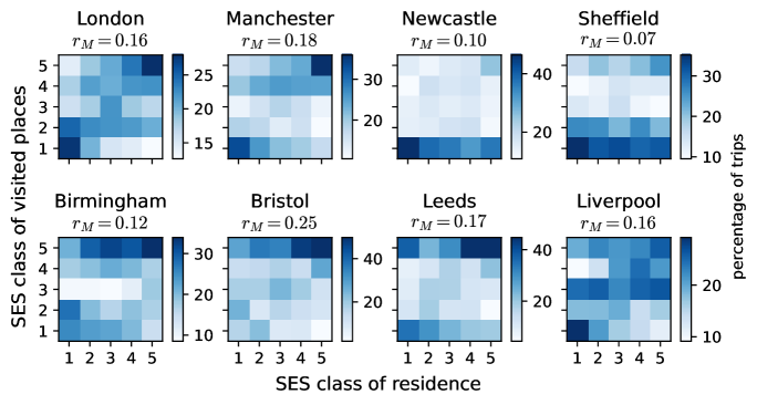
Figure 3: The $M_{k,l}$ mobility mixing matrices stratified by SES in eight metropolitan areas of England. Each matrix is column-wise normalised and depicts the probability for a user who resides in a location of class $l$ (x-axis) to make trips to a place of class $k$ (y-axis). For the definition of $M_{k,l}$, see Eq. 3. For each metropolitan area, we give the $r_{M}$ assortativity coefficient measured from the corresponding mobility mixing matrix, as defined in Eq. 4.

The assortativity level present in these mobility mixing matrices can be quantified by the network assortativity coefficient $r_{M}$, that is defined as the Pearson correlation between values of the rows and columns of the matrix (for precise definition see Materials & Methods). This coefficient takes values between $-1\leq r_{M}\leq 1$. It is negative if people prefer to mix with dissimilar others, it is zero if the mixing is completely random without any bias, and it is positive in case of assortative biases, when people tend to mix with others of similar SES.

The $r_{M}$ assortativity coefficients measured from the corresponding matrices of the studied metropolitan areas are shown in the inset of each matrix in Fig. 3. These were computed for $n_{\sigma}=5$ SE classes. We show in LABEL:SIfig:assortativity_vs_nr_classes the $r_{M}$ values for $n_{\sigma}\in\{3,5,10\}$, which shows the robustness of $r_{M}$ under variation of $n_{\sigma}$ when the latter is high enough. At the same time, they show unexpected correlations when plotted against linguistic measures. Interestingly, as shown in Fig. 4a, mobility mixing assortativity show a clear negative correlation with the average frequency of grammar mistakes measured in the different cities. More mixing thus tends to imply more frequent mistakes, and less segregated populations favour the spread of popularity of non-standard English. Strikingly, in Fig. 4b, another negative correlation was found between the mobility mixing assortativity and the correlation coefficient we measured earlier (see Fig. 2) between SE status and the average frequency of grammar mistakes. This indicates that the stronger the mobility mixing we observe in a population, the less the propensity to deviate from standard rules is determined by the SES of origin. Therefore, the usage of standard English is not only determined by the SE class, but also importantly by the degree of mixing of the populations living in a metropolitan area.

Figure 4: The influence of assortativity on deviations from standard language. (a) The frequency of grammar mistakes seems to rather increase with mixing, although some cities like London or Liverpool deviate quite significantly from this tendency. (b) The dependence on SES of origin clearly decreases as assortativity increases. This means that the more SE classes mix with one another, the less the usage of the standard form of individuals will depend on their own SES. Blue lines indicate the result of a linear regression, with the corresponding Pearson r and p-value given in the two legends. The areas coloured in light blue indicate the $95\text{\,}\mathrm{\char 37\relax}$ confidence interval for the regression estimates.

A model for language adoption

Definition

Having identified the importance of social mixing, our next aim is to understand the mechanisms behind this observation with a simple model. There are three main effects we would like the model to account for:

1. One of the two varieties of the language may be more prestigious than the other. This is for example the case of the standard form: it is taught at schools and spoken by mainstream media and public institutions  (?, ?). This corresponds to what is known as overt prestige.

2. Even though one variety is less prestigious, it might still be preferred by a part of the population that has some kind of cultural attachment to it. For instance, slang can be preferred by members of lower SES, as using it might give them a sense of group identity  (?, ?, ?). This is known as covert prestige.

3. We previously observed very different mixing patterns in various English metropolitan areas. Indeed, mobility can be very heterogeneous, so it should be possible to plug in any mobility data into the model to be able to understand how different mixing may affect the dynamics of the linguistic varieties.

Relevant to our modelling challenge, there are already models for cultural transmission, like the seminal Axelrod model  (?, ?, ?, ?, ?), that could be akin to our desired model for language variety adoption. However, in these models no dependence has been taken into account on an agent’s intrinsic attribute or group identity, thus missing the effect of (ii) in their models. Other works have tried to model the diffusion of dialect features  (?, ?), which could also be considered similar to the dynamics we wish to understand here. But these models consider spatial diffusion with uniform use in areas, which work remarkably well to delimit dialectal regions, but are poorly adapted to fine-grained variations such as the ones we observe within metropolitan areas.

With these considerations in mind, we propose an agent-based model (ABM) as follows. Our model considers agents who are assigned as residents to a cell, which belongs to one of two SE classes. Agents have a linguistic state, which can either comply with the standard rules, or not. The standard form has an intrinsic prestige variable $s$, which can take values from the unit interval. Note that in our case, to comply with effect (i) that we wish to model, we always set $s>0.5$, thus introducing a higher prestige for the standard form. To model effect (ii), each SE class has a preference towards one form: class 1 is biased towards the non-standard form (denoted 1) with a factor $q_{1}$, and inversely class 2 is attached to the standard one (denoted 2) with a factor $q_{2}$. These factors are also constrained between $0$ and $1$, and when they take a value above $0.5$, they represent a bias towards the respective form. For instance, when an agent of class 1 speaking non-standard interacts with another agent speaking standard, they have a probability $s(1-q_{1})$ to start using the standard form as well.

Beyond the language adoption dynamics, we allow agents to move to different cells $j$, according to the probabilities $M_{i,j}$, conditional to their cell of residence $i$. This mechanism controls the mixing of the two populations that we mentioned in (iii). To summarise our model, we show a schematic definition in  Fig. 5.

Figure 5: Schematic summary of model definition. The model features two SE classes, represented by circles and triangles. Agents in each class can speak one of two varieties of their language: the standard form (filled shapes) and the non-standard (empty shapes). Each agent has a cell of residence, and a mobility matrix $M_{i,j}$ that defines the probabilities for a resident of $i$ to be at different cells at each time step. Once an agent is moved, another agent is picked randomly to interact with. If they interact with an agent using the other variety, they adopt this variety with a probability that depends on their SE class of origin. For instance, when a triangle (SES 1) speaking non-standard interacts with another agent from any class speaking standard, they have a probability equal to $s(1-q_{1})$ to adopt the standard form. Possible transitions are presented as arrows between circles and triangles.

Model analysis

Our model can be simulated for any number of cells and arrangements of the populations of different SE classes. However, here we will consider a simple case in order to present succinct equations that lend themselves to interpretation and may lead to a treatable mathematical description. We will consider only two cells, with all individuals of class 1 residing in cell 1, and all individuals of class 2 residing in cell 2. We assign by $p_{1}$ the proportion of individuals of class 1 speaking non-standard (variety 1), and by $p_{2}$ the proportion of individuals of class 2 speaking standard forms (variety 2). Individuals have to speak either 1 or 2, which implies that, for instance, a proportion $(1-p_{1})$ of individuals of class 1 speak the variety 2. These two variables therefore summarise the linguistic state of the system at any given time.

Regarding the mobility, we make the assumption that people of the two classes have the same probability $M$ to move away from their residence cell. Note that this parameter summarises how much the classes mix, as the Pearson $r$ of the mobility matrix in Eq. 4 satisfies $r_{M}=1-2M$. We also assume that the two SE classes have the same population, and we obtain the system of coupled differential equations given by Eq. 5, shown in Materials & Methods. Two opposing effects can be identified in the dynamics of the model in this simple setting.

• The more individuals of different classes mix through their mobility patterns, the smaller the differences in the usage of language varieties between them. This aligns with our observation from Fig. 4b.

• The stronger the bias of a class for its preferred variety, the more homogeneous the variety adoption within this class.

We further determine the states of convergence of the model of Eq. 5. We thus find that the model can not only converge to a state featuring the extinction of one of the two varieties, but also that both may coexist. To illustrate this point, for $M=0.2$, $q_{2}=0.5$, $q_{1}=0.7$, and $s\in\{0.5,0.6,0.7\}$, we show in Fig. 6(a-b-c) the position of the identified fixed points of the model and whether they are stable. These stream plots also demonstrate the dynamics leading to convergence.

Figure 6: Stability analysis of the model dynamics. We analyse the mean-field description of the model, given in Eq. 5, with $q_{2}=0.5$. Stream plots show the fixed points of the model for $M=0.2$, $q_{1}=0.7$ and (a) $s=0.5$, (b) $s=0.6$ and (c) $s=0.7$. The points $(1,0)$ and $(0,1)$ are shown to consistently feature as stable (blue) or unstable (red) fixed points. The first being stable for $s$ significantly lower than $q_{1}$ (a) and the second for $s$ close to or higher than $q_{1}$ (c). A third fixed point featuring coexistence of the two varieties may appear for intermediate values of $s$ (c). In panel (d), after setting $s=0.6$, we show trajectories of the stable fixed points for different values of $q_{1}$, corresponding to the coexistence when varying $M$ from $0$ to $0.5$. This shows how increasing $M$ moves the stable fixed point of coexistence toward the dashed line corresponding to $p_{2}=1-p_{1}$, and towards the extinction of variety 1 or 2 for respectively low or high values of $q_{1}$.

When the attachment to non-standard forms parametrised by $q_{1}$ is significantly higher than the prestige $s$ of the standard variety (as in panel (a)) the stable fixed point corresponds to the dominance of variety 1. At the same time, $q_{1}=s$ implies a stable dominance of variety 2 (as shown in panel (c)). Coexistence of the two varieties is possible for intermediate values of $s<q_{1}$, like for $0.6$ (as shown in panel (b)). As proven in LABEL:SIsec:coex_sol_ses_model, the condition $s<q_{1}$ is actually a strong requirement for the existence of a fixed point corresponding to coexistence. In Fig. 6d, we show how this stable fixed point moves in the $(p_{1},p_{2})$ space when varying $M$, for $s=0.6$ and different values of $q_{1}$. As shown earlier, increasing $M$ pushes the system towards $p_{2}=1-p_{1}$, and whether it is biased towards variety 1 or 2 depends on the difference between $q_{1}$ and $s$. This feature is very much in line with the observation we shared in Fig. 4: the less assortative the mixing – that is the closer $r_{M}$ here is to $0$ – the less the usage of the standard variety depends on SES – which in our case means that $(1-p_{1})$ will get closer to $p_{2}$.

In Fig. 7 we present the regions of the $(q_{1},M)$ parameter space where the aforementioned stable solutions appear. For a prestige favouring variety 2 ($s>0.5$), but with a value still low enough (as in panel (a)), three distinct domains appear in the parameter space: two corresponding to dominance of one variety and extinction of the other, and a third corresponding to coexistence of the two varieties. At the same time, higher values of $s$ prohibit stable solutions associated to the dominance of 1, as shown in panel (b). Coexistence is facilitated by less mixing between the different classes, yet for a given range of values of $q_{1}$, no matter how much populations mix, the two varieties can still coexist. This is noteworthy result as while segregation leads to the conservation of varieties, we find that coexistence is still possible regardless of the mixing.

Figure 7: Parameter space of the model in a simple setting split by the kind of stable fixed points. Solutions of the mean-field model is shown defined in Eq. 5, with $q_{2}$ set at the neutral value of $0.5$. The regions of the $(q_{1},M)$ parameter space are depicted where different kinds of stable solutions emerge, with (a) $s=0.6$ and (b) $s=0.7$. Regions correspond to three possible stable fixed points: the extinction of variety 2 and dominance of 1 labelled with “non-standard only”, inversely the dominance of 2 labelled with “standard only”, and the coexistence of both varieties labelled with “coexistence”. Examples for each of these are respectively shown in Fig. 6(a-c-b). Stable coexistence of varieties 1 and 2 is favoured for rather low mobility and a preference of class 1 for variety 1 $q_{1}$ higher than the second variety’s prestige $s$.

Data-driven simulation for metropolitan areas

The rich phenomenology that the model exhibits calls for a further investigation to see if it can reproduce the empirically observed correlations between assortativity and language varieties, once initialised with real parameters. We run simulations in each of the eight metropolitan areas analysed in Figs. 3 and 4. We populate their MSOAs with as many agents as they have inhabitants according to the census, and attribute the average income also given by the census to all agents of each area. In these simulations, we consider five SE classes, that we can compare results directly to the outputs of our data analysis, shown in Fig. 4. To fully parameterise the model, we need three more linguistic parameters, namely the preferences for one of the two language varieties for each additional class. In order to limit the number of parameters to explore, we only keep the preferences $q_{1}$ and $q_{2}$, which set the preference of class 1 (the poorest) for variety 1 and of class 5 (the richest) for variety 2. Meanwhile, to attribute preferences for variety 1 to each remaining class, we use a linear interpolation between $q_{1}$ and $1-q_{2}$. To be consistent with the phenomenon we are interested in, this interpolation is always a decreasing function of the class number, as we run simulations with $q_{1}>0.5$ and $q_{2}\geq 0.5$. To avoid the uninteresting states of convergence featuring a hegemony of standard language, we only consider values of the prestige such that $s>0.5$ and $q_{1}>s$. Thus, the only feature left as unknown parameter for the simulations is the inter-cell mobility of the agents. To estimate this parameter, we leverage the mobility we observed from Twitter data, the $t_{u,c}$ we introduced previously, but this time including the travels of the users within their own cell of residence. We thus obtain a matrix giving for each cell the probability for their residents to be found in any cell at each simulation step. In summary, at most three random draws are performed at each step for each agent: i) to decide in which cell this agent will be interacting with others; ii) to choose the other agent they will interact with; and if the two are using different varieties, iii) to decide whether they will switch, according to their class switch probability (similarly to what is depicted in Fig. 5 for just two classes). A sample result from our simulations is given in Fig. 8.

Figure 8: Sample result from the ABM simulations in eight metropolitan areas. Correlation between the average income and proportion of speakers choosing variety 1 at the stable state of convergence of the simulations for $s=0.55$, $q_{1}=0.7$ and $q_{2}=0.5$ against the cities’ assortativity. This example was selected for having one of the lowest correlations between x and y-axis values, which are shown for other values of $q_{1}$ and $s$ in LABEL:SIfig:phase_space_ses_city_sims.

The original aim of the proposed model was to better understand how social mixing facilitates the interdependence between SES and the usage of standard language, as shown in Fig. 4. To synthesise an answer to this challenge, at the stable state reached by the simulations in each city, we measure in each cell the proportion of agents using the non-standard language variety 1. Similarly to the data analysis, we compute the correlation between the cells’ average income and the proportion of agents using the non-standard form, and check it against the measured assortativity of the different cities (for model parameter values see the caption of Fig. 8). By comparing Fig. 8 with the corresponding empirical results in Fig. 4 we find striking similarities between the observed and modelled correlations, that verifies the modelled mechanisms to give a possible explanation for the observed phenomena. Note that due to the two different proxies for the usage of non-standard language, beyond the observed negative correlations, we do not expect the absolute values of the y-axes to match. The parameter set that led to the result of Fig. 8 was not chosen arbitrarily. Indeed, to find the best parametrization that most closely reproduce the empirical observations, we performed a grid search in the parameter space with an increment of $0.05$ in parameter values. These are shown in LABEL:SIfig:phase_space_ses_city_sims. As visible in LABEL:SIfig:phase_space_ses_city_simsa, to avoid states of convergence that are irrelevant to us (featuring the extinction of variety 1), simulations were run only for values of $q_{1}$ strictly superior to $s$. This panel depicts correlation values computed between the axis of plots similar to Fig. 8, but for different parameter values. The highest absolute correlation value in this plot correspond to $s=0.55$, $q_{1}=0.7$ and $q_{2}=0.5$. The $r$ values are shown in LABEL:SIfig:phase_space_ses_city_sims(a-b) for $q_{2}=0.5$ and $s=0.55$, respectively. The two panels clearly demonstrate that the empirically-observed correlation pattern can be robustly reproduced for several parameter values, which lead to stable states featuring $r$ values relatively close to $-1$. Consequently, our simple model with only three parameters is able to capture our empirical observations with notable precision.

Discussion

Throughout this work, we have investigated the inter-dependence between SES and the usage of different linguistic varieties. Focusing on the dichotomy between standard and non-standard English usage in England and Wales, through a combination of Twitter and census data we found that the average frequency of grammar mistakes and average income are slightly correlated. More interesting though is that across eight metropolitan areas, the more different SE classes mix together, the weaker this correlation, meaning the more similar the usage of English across classes.

We have subsequently introduced an ABM that proposes an explanation for this observation. It features transition probabilities from using one variety to the other that depend on both a globally shared overt prestige of the standard, and a class-dependent covert prestige — or preference — for one of the two. We have here shown that the preferential attachment of a group for a linguistic feature can be crucial to sustain it, despite an unfavourable prestige. The analytic framework we presented here has the virtue of enabling us to capture the role of social mixing between these different groups. In accordance with our observations made with Twitter data, we have shown analytically that it tends to smooth out linguistic differences between SE classes. Remarkably, this smoothing does not necessarily imply homogeneous language, but may also mean comparable prominence of the two linguistic varieties of the two groups. These analytic findings are also supported by the results of agent-based simulations involving the populations of the eight metropolitan areas we studied empirically. The simulations can yield the same relationship we obtained from the data, namely that the more social mixing there is across socioeconomic classes, the less the individuals’ choice to use standard or non-standard language will depend on their class of origin.

This work provides a solid foundation for future works of the same vein. It could first be extended to other countries where similar data could be obtained in sufficient amounts. Also, our observations were made in the social context of Twitter, but individuals may choose to use a different language in other environments. This potential change of behaviour is therefore not captured by our model, but it could be relevant to the global dynamics. Observing the language production of individuals in different social contexts on a scale such as the one we presented here poses a great challenge, but it would definitely help further modelling endeavour and thus greatly contribute to our understanding of these linguistic phenomena.

Materials & Methods

Filtering Twitter users

As we are interested in the natural speech, we start our analysis by filtering out users whose behaviour resembles that of a bot. We first eliminate those tweeting at an inhuman rate, set at an average of ten tweets per hour over their whole tweeting period. Then, we only keep those who only tweeted either from a Twitter official app, Instagram, Foursquare or Tweetbot — a popular third-party app. These were selected because they are significantly popular among real users. Also, consecutive geolocations implying speeds higher than a plane’s ($1000\text{\,}\mathrm{km}\text{\,}{\mathrm{h}}^{-1}$) are detected to discard users. Finally, in order to only keep residents of England and Wales, we impose that users must have tweeted from there in at least three consecutive months.

Residence attribution

Tweets’ geotags can be given at different geographical levels. Some tweets include coordinates, which were more abundant prior to 2015, when the network changed their geolocation policy. From the end of 2015 on, it has become more common to have geotags at the level of places. Places are geographical areas that may go from full countries, to regions or provinces, cities, neighbourhoods or even points of interest.

Since the sizes of these places span orders of magnitude, some may intersect many cells. There can then be so much uncertainty in the actual geographic origin of the tweet that it is preferable to discard it. Our criterion here is that when the top four cells which contain most of the place’s area do not contain more than $90\text{\,}\mathrm{\char 37\relax}$ of its total area when put together, the place, and all the tweets assigned to it, are discarded.

Now, to explain the heuristics we defined for residence attribution, let us first formalise some notation. The tweets of a user $u$ attributed to a cell $c$ are the sum of those with coordinates and those with a place intersecting $c$. If the tweets’ place intersects several cells, then we apply the following criterion to calculate the contribution to $c$:

$$r_{c}=\sum_{p}n_{p}\frac{A_{p\cap c}}{A_{p}},$$ (1)

where $n_{p}$ are the tweets in place $p$, $A_{p}$ is the area of $p$ and $A_{p\cap c}$ is the area of the intersection between $p$ and $c$.

The cell of residence of each user is thus the one from which they tweet more often between 6pm and 8am. Besides, we also impose that the user must have tweeted at least three times and at least $10\text{\,}\mathrm{\char 37\relax}$ of the time from that cell, and that at night the majority of their tweets were from there. All users for whom a cell of residence could not be attributed are subsequently discarded from the analysis.

Tweet processing

Since we are interested in the speech, we need to clean parts of the text which cannot be considered as natural language production. Those are the URLs, mentions of other users and hashtags. It is not completely obvious that the latter should be discarded though. Hashtags are used on Twitter to aggregate tweets by topics. It is an important feature of the website, whose aim is to enable users to easily find the tweets of other users discussing similar topics, or inversely to make one’s tweets more discoverable by others, and to see real time trends on the platform. Hence, there can be completely different motivations behind writing a hashtag: to actually tag a tweet with one or more topic, to promote the tweet, or simply follow a trend. Thus, the content of hashtags can deviate significantly from normal speech  (?). It is therefore safer to discard hashtags entirely, which is no issue as long as we can collect enough textual content without them anyway. We actually made some measurements in our tweets’ database to see if that was the case. We took several random samples of a million tweets each, stripped them of URLs and mentions, and then computed the ratio of characters within a hashtag compared to the total number of characters left in those tweets. This proportion was found to be consistently below $5\text{\,}\mathrm{\char 37\relax}$. We thus consider the precaution of stripping hashtags off of tweets worth taking. After this cleaning step, for what follows we then keep only the tweets still containing at least four words. The next crucial step is to infer the language the tweets are written in. To do so, we leverage a trained neural network model for language identification: the Compact Language Detector  (?), whose output is a language prediction along with the confidence of the model. Subsequently, we only keep tweets detected as having been written in English with a confidence above $90\text{\,}\mathrm{\char 37\relax}$.

Definition of socioeconomic classes

Since the assigned SES indicator, i.e. average income, is the same for every user living in the same MSOA, they will be all necessarily assigned to the same class. Considering the cells in a given metropolitan area, we rank them by increasing average net income. We get their population from the census, denoted $N_{c}$ for each cell $c$ in the following. Denoting $I_{c}$ the set of cells with an average income lower than or equal to $c$’s, we determine the SE class of $c$ as:

$$\sigma_{c}=n_{\sigma}\left\lceil\frac{\sum_{c^{\prime}\in I_{c}}N_{c^{\prime}}}{\sum_{c^{\prime}}N_{c^{\prime}}}\right\rceil,$$ (2)

with $\left\lceil\cdot\right\rceil$ representing the ceiling function and $n_{\sigma}$ the number of classes we wish to define. $\sigma_{c}$ takes integer values between $1$ and $n_{\sigma}$, both included, the former corresponding to the cells of lowest income, and the latter to the ones of highest income.

Definition of mobility mixing matrix and assortativity

From our corpus of geotagged tweets, for every user $u$ we compute the proportion of tweets made by them that fall within each cell $c$, denoted $t_{u,c}$. This allows us to introduce the probability for an individual to visit a cell of class $k$ knowing that they reside in a cell of class $l$:

$$M_{k,l}=\frac{\sum_{c^{*}\in S_{l}}\sum_{u\in c^{*}}\sum_{c\in S_{k}}t^{*}_{u,c}}{\sum_{c^{*}\in S_{l}}\sum_{u\in c^{*}}\sum_{k^{\prime}=1}^{n_{\sigma}}\sum_{c\in S_{k^{\prime}}}t^{*}_{u,c}},$$ (3)

where $t^{*}_{u,c}$ is $t_{u,c}$ but set to zero for $c=c_{u}^{*}$, $c_{u}^{*}$ being the residence cell of user $u$, and renormalised so that $\sum_{c}t^{*}_{u,c}=1$ for every user. The $M_{k,l}$ form a column-wise normalised matrix, meaning $\sum_{k}M_{k,l}=1$. We here use the proportions $t^{*}_{u,c}$ instead of raw counts so as to make every user of a class contribute equally to $M_{k,l}$, thus accounting for the wide range of activity distributions.

Assortative patterns can be summarised by a measure of how strongly diagonal these matrices are: their Pearson r value, denoted $r_{M}$ here. It is defined as follows:

$$r_{M}=\frac{N_{M}\sum_{k,l}klM_{k,l}-\sum_{k,l}kM_{k,l}\cdot\sum_{k,l}lM_{k,l}}{\sqrt{N_{M}\sum_{k,l}k^{2}M_{k,l}-\left(\sum_{k,l}kM_{k,l}\right)^{2}}\cdot\sqrt{N_{M}\sum_{k,l}l^{2}M_{k,l}-\left(\sum_{k,l}lM_{k,l}\right)^{2}}},$$ (4)

with $N_{M}=\sum_{k,l}M_{k,l}$, which is equal to the number of classes $n_{\sigma}$, by definition.

Analysis of the model in mean-field

Following the steps detailed in SI LABEL:SIsec:model_analytic, and using all the assumptions specified there, we can describe our model with the following system of coupled differential equations:

$$\left\{\begin{aligned} \derivative{p_{1}}{t}&=2M(1-M)(1-p_{1}-p_{2})[q_{1}(1-s)-p_{1}(q_{1}-s)]+p_{1}(1-p_{1})(q_{1}-s)\\[4.30554pt] \derivative{p_{2}}{t}&=2M(1-M)(1-p_{1}-p_{2})[q_{2}s-p_{2}(s+q_{2}-1)]+p_{2}(1-p_{2})(s+q_{2}-1)\end{aligned}\right.$$ (5)

Here, we assume that speakers’ interactions are all-to-all. In other words, we adopt as a mean-field approximation, which is a good approximation when considering large populations.

Interestingly, each equation features a first term linked to the group mobility, maximum for $M=\frac{1}{2}$, which describes maximum mixing. This term disappears when $p_{1}=1-p_{2}$ and leads to convergence in the usage of language varieties between SE classes. Indeed, in the first equation, if $q_{1}\leq s$, the term in square brackets is clearly strictly positive. If $q_{1}>s$, we have

$$q_{1}(1-s)-p_{1}(q_{1}-s)>q_{1}(1-s)-(q_{1}-s)=s(1-q_{1})>0.$$ (6)

As a consequence, the sign of the mobility term follows the one of $(1-p_{1}-p_{2})$. It is therefore negative if $p_{1}>1-p_{2}$ and positive otherwise, thus pushing $p_{1}$ towards $1-p_{2}$. Similarly, in the second equation, since $q_{2}s-q_{2}-s>-1$, the mobility term pushes $p_{2}$ towards $1-p_{1}$.

The second term of each evolution equation represents “self-growth”, independent of mobility and maximum for $p_{k}=\frac{1}{2}$. This term thus brings a given class $k$ towards homogeneity. For $k=1$ for instance, it does it either towards $p_{1}=0$ for $q_{1}<s$, or towards $p_{1}=1$ for $q_{1}>s$. When there is no mixing, for $M=0$ or $M=1$, as expected the two populations become completely independent, and the only stable fixed points of the system correspond to homogeneous populations in terms of the language variety they use. The emerging dominant variety depends on the sign of $(q_{1}-s)$ and $(s+q_{2}-1)$ for classes 1 and 2, respectively.

To characterise the fixed points of this system of equations, we also perform a stability analysis. There are two fixed points that can be trivially found from Eq. 5: $(p_{1},p_{2})=(0,1)$ and $(1,0)$. Other fixed points are located using symbolic computations. Then, to determine whether this fixed points are stable states of convergence of the system, we compute the eigenvalues of the Jacobian of the system evaluated at its fixed points. The stable fixed points are those whose corresponding eigenvalues have a strictly negative real part.

Funding: This work was partially supported by the Spanish State Research Agency (MCIN/AEI/10.13039/501100011033) and FEDER (UE) under project APASOS (PID2021-122256NB-C21 and PID2021-122256NB-C22) and the María de Maeztu project CEX2021-001164-M and by the Comunitat Autonoma de les Illes Balears through the Direcció General de Política Universitària i Recerca with funds from the Tourist Stay Tax Law ITS 2017-006 (PDR2020/51). TL is grateful for the support from the EMOMAP CIVICA project. MK was supported by the CHIST-ERA project SAI: FWF I 5205-N; the SoBigData++ H2020-871042; the EPO and EMOMAP CIVICA projects and the DATAREDUX project, ANR19-CE46-0008.

Competing Interests: The authors declare that they have no competing interests.

Data and Materials Availability: All aggregated data we have produced for this paper will be deposited in an Open Science Framework repository upon journal publication. The boundaries of the MSOAs of England and Wales can be downloaded from the Open Geography portal of the Office for National Statistics: https://geoportal.statistics.gov.uk/maps/msoa-dec-2011-boundaries-generalised-clipped-bgc-ew-v3. The estimates of the 2018 census for the net annual income of the MSOAs of England and Wales can be downloaded from https://www.ons.gov.uk/employmentandlabourmarket/peopleinwork/earningsandworkinghours/datasets/smallareaincomeestimatesformiddlelayersuperoutputareasenglandandwales, while their population can be obtained from https://www.nomisweb.co.uk/census/2011/ks101uk. All code needed to reproduce the results in the paper is deposited in public GitHub repositories: at https://github.com/TLouf/ses-ling for Python code used to analyse data, run the simulations and produce all figures except Figs. 6 and 7, and at https://github.com/TLouf/ses-ling-analytical for Mathematica code used to analyse our model in mean-field and produce the two aforementioned figures.

References

- 1. I. L. Pedersen, in Dialect Change: Convergence and Divergence in European Languages, P. Auer, F. Hinskens, P. Kerswill, Eds. (Cambridge University Press, Cambridge, UK, 2005).
- 2. P. Bourdieu, Language and Symbolic Power (Polity Press, Cambridge, UK, 2009).
- 3. W. Labov, The Social Stratification of English in New York City (Cambridge University Press, Cambridge, UK, 1966).
- 4. P. Trudgill, The Social Differentiation of English in Norwich, no. 13 in Cambridge Studies in Linguistics (Cambridge University Press, Cambridge, UK, 1974).
- 5. T. Louf, D. Sánchez, J. J. Ramasco, Capturing the diversity of multilingual societies. Physical Review Research 3, 043146 (2021).
- 6. S. Romaine, in The Handbook of Bilingualism and Multilingualism: Second Edition (John Wiley & Sons, Ltd, Chichester, UK, 2012), pp. 443–465.
- 7. P. Garrett, in The Routledge Companion to Sociolinguistics, C. Llamas, L. Mullany, P. Stockwell, Eds. (Routledge, London, UK, 2006), pp. 136–141.
- 8. W. A. Kretzschmar, Jr., Language Variation and Complex Systems. American Speech 85, 263–286 (2010).
- 9. J. K. Chambers, P. Trudgill, in Dialectology (Cambridge University Press, Cambridge, UK, 2004), pp. 57–69, second edn.
- 10. P. Foulkes, G. Docherty, Eds., Urban Voices: Accent Studies in the British Isles (Routledge, London, 2014).
- 11. J. K. Chambers, Sociolinguistic Theory: Linguistic Variation and Its Social Significance, no. 22 in Language in Society (Blackwell, Malden, MA, USA, 2007), second edn.
- 12. OECD, Where All Students Can Succeed, vol. II of PISA 2018 Results (OECD Publishing, Paris, FR, 2019).
- 13. J. Gao, Y.-C. Zhang, T. Zhou, Computational socioeconomics. Physics Reports 817, 1–104 (2019).
- 14. J. Eisenstein, B. O’Connor, N. A. Smith, E. P. Xing, Diffusion of lexical change in social media. PLoS ONE 9, e113114 (2014).
- 15. B. Gonçalves, D. Sánchez, Crowdsourcing dialect characterization through Twitter. PLOS ONE 9, e112074 (2014).
- 16. E. Bokányi, D. Kondor, L. Dobos, T. Sebők, J. Stéger, I. Csabai, G. Vattay, Race, religion and the city: Twitter word frequency patterns reveal dominant demographic dimensions in the United States. Palgrave Communications 2, 1–9 (2016).
- 17. G. Donoso, D. Sánchez, Dialectometric analysis of language variation in Twitter, in Proceedings of the Fourth Workshop on NLP for Similar Languages, Varieties and Dialects (VarDial) (Association for Computational Linguistics (ACL), Valencia, Spain, 2017), pp. 16–25.
- 18. J. Grieve, C. Montgomery, A. Nini, A. Murakami, D. Guo, Mapping lexical dialect variation in British English using Twitter. Frontiers in Artificial Intelligence 2, 11 (2019).
- 19. T. Louf, B. Gonçalves, J. J. Ramasco, D. Sánchez, J. Grieve, American cultural regions mapped through the lexical analysis of social media. Humanities and Social Sciences Communications 10, 1–11 (2023).
- 20. S. Šćepanović, I. Mishkovski, B. Gonçalves, T. H. Nguyen, P. Hui, Semantic homophily in online communication: Evidence from Twitter. Online Social Networks and Media 2, 1–18 (2017).
- 21. M. Martinc, P. Kralj Novak, S. Pollak, Leveraging Contextual Embeddings for Detecting Diachronic Semantic Shift, in Proceedings of the Twelfth Language Resources and Evaluation Conference (European Language Resources Association, Marseille, France, 2020), pp. 4811–4819.
- 22. J. Eisenstein, Systematic patterning in phonologically-motivated orthographic variation. Journal of Sociolinguistics 19, 161–188 (2015).
- 23. A. K. Jørgensen, D. Hovy, A. Søgaard, Challenges of studying and processing dialects in social media. ACL-IJCNLP 2015 - Workshop on Noisy User-Generated Text, WNUT 2015 - Proceedings of the Workshop pp. 9–18 (2015).
- 24. B. Gonçalves, L. Loureiro-Porto, J. J. Ramasco, D. Sánchez, Mapping the americanization of English in space and time. PLOS ONE 13, e0197741 (2018).
- 25. J. L. Abitbol, M. Karsai, J.-P. Magué, J.-P. Chevrot, E. Fleury, Socioeconomic dependencies of linguistic patterns in twitter: A multivariate analysis, in Proceedings of the 2018 World Wide Web Conference, WWW ’18 (International World Wide Web Conferences Steering Committee, Republic and Canton of Geneva, Switzerland, 2018), pp. 1125–1134.
- 26. D. Mocanu, A. Baronchelli, N. Perra, B. Gonçalves, Q. Zhang, A. Vespignani, The Twitter of Babel: Mapping world languages through microblogging platforms. PLoS ONE 8, e61981 (2013).
- 27. A. Mislove, S. Lehmann, Y.-Y. Ahn, J.-P. Onnela, J. N. Rosenquist, Understanding the demographics of Twitter users, in Proceedings of the International AAAI Conference on Web and Social Media (AAAI Press, Barcelona, 2011), vol. 5, pp. 554–557.
- 28. R. M. Hilman, G. Iñiguez, M. Karsai, Socioeconomic biases in urban mixing patterns of US metropolitan areas. EPJ Data Science 11, 1–18 (2022).
- 29. B. Davila, The Inevitability of “Standard” English: Discursive Constructions of Standard Language Ideologies. Written Communication 33, 127–148 (2016).
- 30. J. Milroy, in The Routledge Companion to Sociolinguistics, C. Llamas, L. Mullany, P. Stockwell, Eds. (Routledge, London, UK, 2006), pp. 153–159.
- 31. R. Axelrod, The Dissemination of Culture: A Model with Local Convergence and Global Polarization. The Journal of Conflict Resolution 41, 203–226 (1997).
- 32. C. Castellano, M. Marsili, A. Vespignani, Nonequilibrium Phase Transition in a Model for Social Influence. Physical Review Letters 85, 3536–3539 (2000).
- 33. K. Klemm, V. M. Eguíluz, R. Toral, M. S. Miguel, Global culture: A noise-induced transition in finite systems. Physical Review E 67, 045101 (2003).
- 34. K. Klemm, V. M. Eguíluz, R. Toral, M. San Miguel, Nonequilibrium transitions in complex networks: A model of social interaction. Physical Review E 67, 026120 (2003).
- 35. F. Battiston, V. Nicosia, V. Latora, M. Miguel, Layered social influence promotes multiculturality in the Axelrod model. Scientific Reports 7 (2017).
- 36. J. Burridge, Spatial evolution of human dialects. Physical Review X 7, 031008 (2017).
- 37. J. Burridge, T. Blaxter, Inferring the drivers of language change using spatial models. Journal of Physics: Complexity 2, 035018 (2021).
- 38. R. Page, The linguistics of self-branding and micro-celebrity in Twitter: The role of hashtags. Discourse & Communication 6, 181–201 (2012).
- 39. A. Salcianu, A. Golding, A. Bakalov, C. Alberti, D. Andor, D. Weiss, E. Pitler, G. Coppola, J. Riesa, K. Ganchev, M. Ringgaard, N. Hua, R. McDonald, S. Petrov, S. Istrate, T. Koo, Compact language detector v3 (CLD3) (2023). URL: https://github.com/google/cld3/.