TbExplain: A Text-based Explanation Method for Scene Classification Models with the Statistical Prediction Correction

Abstract

The field of Explainable Artificial Intelligence (XAI) aims to improve the interpretability of black-box machine learning models. Building a heatmap based on the importance value of input features is a popular method for explaining the underlying functions of such models in producing their predictions. Heatmaps are almost understandable to humans, yet they are not without flaws. Non-expert users, for example, may not fully understand the logic of heatmaps (the logic in which relevant pixels to the model’s prediction are highlighted with different intensities or colors). Additionally, objects and regions of the input image that are relevant to the model prediction are frequently not entirely differentiated by heatmaps. In this paper, we propose a framework called TbExplain that employs XAI techniques and a pre-trained object detector to present text-based explanations of scene classification models. Moreover, TbExplain incorporates a novel method to correct predictions and textually explain them based on the statistics of objects in the input image when the initial prediction is unreliable. To assess the trustworthiness and validity of the text-based explanations, we conducted a qualitative experiment, and the findings indicated that these explanations are sufficiently reliable. Furthermore, our quantitative and qualitative experiments on TbExplain with scene classification datasets reveal an improvement in classification accuracy over ResNet variants.

[inst1]organization=School of Computer Engineering,addressline=Iran University of Science and Technology, country=Iran

[inst2]organization=Department of Computer Engineering,addressline=Sharif University of Technology, country=Iran

[inst3]organization=School of Computer Science and Engineering,addressline=Nanyang Technological University, country=Singapore

1 Introduction

Image classification aims to categorize an input image among the predefined class memberships (like animals, vehicles, furniture, diseases, etc.) [1]. As a fundamental task in computer vision, image classification supports a broad range of applications, such as disease diagnosis, remote sensing, and robotics [2, 3, 4]. State-of-the-art architectures, such as ResNet [5], have progressed to the point where they even surpass human-level performance [6]. The traditional machine learning methods, such as Support Vector Machines (SVM) [7], lack the ability to efficiently and automatically extract features from the input images, handle two-dimensional image data, and effectively capture discriminating features, which are crucial for facilitating classification tasks. Conversely, requiring minimal manual engineering, deep learning promotes suitable feature extraction and powerfully extracts important information by transforming the data into a high representation level and learning characteristics of the input that are essential for accurate discrimination between images of different categories [8, 9].

Since the standard Feed-Forward Networks are limited in efficiently capturing local information and are susceptible to over-fitting and gradient vanishing with the increase of their layers, Convolutional Neural Networks (CNNs) attracted the attention of researchers to overcome these challenges. As a class of Deep Learning Neural Networks (DNN), CNNs are ideal tools that have proven supremacy in image processing and have made major contributions to the field of computer vision as a result of their capacity to capture representative features without human supervision [10, 11]. CNNs gain advantages over traditional neural networks by incorporating pooling and weight sharing to reduce feature map dimensions, lessen computational effort, facilitate generalization, and avoid over-fitting [9, 12, 13]. In image classification, CNN aims to learn discriminating features from input images so that samples from different classes are pushed further apart in the representation space, followed by a dense layer that performs the classification. There have been remarkable research efforts in CNN-based image classification. Numerous algorithms have been proposed to compete in the ImageNet Large Scale Visual Recognition Challenge (ILSVRC) [14] as image classification models to demonstrate their classification performance on the ImageNet dataset, including VGG [15], GoogLeNet [16], and ResNet [5]. We choose ResNet as the ILSVRC 2015 winner to perform image classification in our proposed framework.

Contrary to all the advantages mentioned for deep models, since they are over-parameterized and black-box, it is often difficult to decipher how predictions are generated by them [17, 18]. This challenge is associated with a "lack of interpretability" issue that prevents the adoption of deep models in sensitive applications due to a lack of trust in their output generation process [19]. Due to the obscurity of deep models’ inner mechanisms and functions, it is also challenging to diagnose and debug them [20, 21]. Ultimately, the lack of interpretability of a deep model restricts its user from comprehending the reasoning behind its predictions, resulting in a decline in its usage. Also mentioned in some literature is the concept of explainability, which in most previous papers is considered synonymous with interpretability. Still, in others, its definition is distinct from that of interpretability. For instance, the authors of [22] elucidate the difference between these two concepts as: Explainability refers to models that can encapsulate the rationale for neural network activity, earn the trust of users, or generate insights into the reasoning behind their actions. By default, interpretable models are explainable, although this is not always the case.

Both industry and academia have paid considerable attention to model interpretability and post hoc explanation methods in recent years. Numerous intrinsically interpretable models [23, 24, 25, 26] and post hoc explanation methods [27, 28, 29], for models that cannot be interpreted on their own, have been proposed in prior literature. There are various fields in which XAI methods can be helpful to obtain advantageous information about the input features’ relevance to the final output [30]. For instance, in the context of natural language processing, XAI techniques have been used to quantify the effect of various language features in prediction models for sentiment analysis [31], depression detection [32], metaphor understanding [33], personality detection [34], and more. The generation of a saliency map [35] (also known as heatmap) on the model’s input features is one of the most often employed XAI approaches for deep models. A saliency map allows for the assessment and observation of the input features’ importance and relevance in the model’s prediction. However, they may not be accurate enough for users who do not grasp the rationale of the heatmap. For instance, they may not comprehend the correlation between an input feature and the model’s output. In addition, objects and regions of the input image that are relevant to the model prediction are frequently not entirely differentiated by heatmaps. In other words, the areas specified by the heatmap may be fragmented and dispersed, preventing the user from accurately recognizing them in the image that prompted this prediction.

In this paper, we present a novel method for explaining textually the underlying rationale of a scene classification model. This method combines a pre-trained object recognition model and a saliency-based explanation technique to provide a textual response to the question of what objects are present in the input image for which the model generated the specific prediction. This method eliminates the drawbacks of heatmaps since the user can easily recognize in textual format which items and regions the model considered in the prediction process. Also, the problem of dispersion and non-uniformity of the relevant regions in heatmaps is not present in this method because, using an embedded module, only objects for which a minimum fraction of them have been considered by the model are presented in the final output.

We further improved classification performance by devising a systematic approach to increase the accuracy of predictions and promote better generalization. Our approach consists of a confidence measure to logically determine whether the output of the image classification module is reliable or not. We designed a logic-based decision maker that statistically learns weights for each object in the training stage by incrementally calculating the probability of the object occurring in each class. In the test stage, if the predicted class by the ResNet meets the confidence threshold, then it is considered the output class. Otherwise, we incorporate a weighted scoring system that allows the decision maker to decide the class of the input image by selecting the class with the highest score according to the statistical quantity of the existing objects in each class. There also exists a third scenario in which neither of the aforementioned outputs can be trusted, so the explanation emphasizes on the unreliability of the output instead. The contribution and novelty of this work are summarized as follows:

• We propose a novel framework designed to offer context-based textual explanations with the goal of improving the interpretability of the underlying mechanisms of scene classification models for non-expert users.

• We present a heuristic-based method called statistical prediction correction (SPC) to obtain a textually explainable revised prediction based on the statistics (count) of objects in the input image when the original prediction is unreliable.

• We conduct qualitative analysis to assess the reliability and trustworthiness of TbExplain’s text-based explanations, which involves comparing the content of these explanations to the manually annotated labels. Furthermore, quantitative experiments on three benchmark scene datasets demonstrate better classification accuracy compared to ResNet.

The remaining sections are organized as follows. In section 2, we discuss the necessary background concepts for understanding the subsequent sections. Section 3 includes the most recent and closely related works to this work. In section 4, we suggest and discuss our proposed framework in detail. In section 5, we explain the setup and results of our experiments. In section 6, we explore the limitations of our study and make recommendations for further research in this domain. Finally, In section 7, we provide concluding remarks.

2 Background and scope

2.1 Object detection

Object detection is the process of recognizing and locating objects in visual data by placing bounding boxes around them. Object detectors use the image as the input to produce the bounding box and the category label for $n$ distinct objects based on the extracted features from the image by employing a backbone architecture. Bounding boxes are rectangles drawn around an object in the image based on the detected spatial properties, including the rectangle’s width, height, and center coordinates. Frameworks for object detection are separated into two categories:

• Single-Stage detectors, which predict the bounding boxes and the categories in a single step without separating the detection proposal process.

• Two-Stage detectors, aiming to generate object proposals before determining their category and before localizing them in the image.

Even though two-stage frameworks usually promote higher accuracy than single-stage detectors, they take longer to produce object proposals and implement complex architectures. In the following, we describe the mechanism of YOLOv5 [36] since we used it as the object detection model in our experiments.

YOLOv5, a single-stage detector, is an extension of the YOLO [37] architecture that promotes higher accuracy in object detection. It is capable of detecting multiple objects in a single image, which means that as well as predicting the classes of these objects, it also identifies their spatial properties. In contrast to previous releases, it employs the PyTorch framework and utilizes the path aggregation network (PANet) [38] as neck to facilitate data flow. YOLOv5 architecture adopts the same problem formulation as previous releases and predicts the four coordinates for bounding boxes, including $t_{x}$ and $t_{y}$ ($x$ and $y$ axis values), $t_{w}$ (width), and $t_{h}$ (height) of the rectangle, by utilizing anchor boxes. To calculate the real width and height of the bounding boxes, offsets to anchors are also calculated, which are denoted by $c_{x}$ and $c_{y}$. The following equations are utilized for calculating the center (x and y), width, and height coordinates of the bounding boxes:

$$b_{x}=\sigma(t_{x})+c_{x}$$ (1)

$$b_{y}=\sigma(t_{y})+c_{y}$$ (2)

$$b_{w}=p_{w}e^{t_{w}}$$ (3)

$$b_{h}=p_{h}e^{t_{h}}$$ (4)

An objectness score for each bounding box is predicted by utilizing logistic regression, which represents the probability of a cell being the center cell that predicts an object. The score equals 1 if the anchor box overlaps a ground truth object by more than any other anchor box. To avoid selecting overlapping boxes, IoU (Intersection over Union) and Non-Max Suppression are implemented.

2.2 Image classification

Image classification is the process of recognizing an image as a whole and assigning a specific label to it. Contrary to object detection, the input images of classification frameworks are typically composed of single objects, and the task only involves classification without the localization part. In the following, we describe the mechanism of ResNet [5] since we used it as the scene classification model in our experiments.

ResNet, which alleviated the degradation problem, is adopted with regard to the image classification step. Simply stacking layers and using deeper networks doesn’t result in higher performance or lower train and test error rates. This work denoted any desired mapping by $H(x)$ and modified the plain architecture as follows: It used skip-connection to avoid activating a layer across one or more layers in the network. Each of these sections that pass over the input of the next layer over multiple layers is considered a residual block. This formulation causes the output of the last layer in the block to change from $H(x)=f(wx+b)$ to the $H(x)=f(wx+b)+x$ format, since the input of the block is also added to its output. Implementing these skip connections into the network provides the ability to skip the layers that hurt performance through regularization. This facilitates the training of deeper architectures by expediting the learning process and avoiding the drop in performance caused by reducing the impact of vanishing gradients. As mentioned before, the experiments were based on the ResNet101V2 variant [39], which contains 101 layers and differs from version one in the use of batch normalization before every weight layer and in removing the non-linearity after the addition operation.

2.3 Explainable Artificial Intelligence (XAI)

Explainable artificial intelligence (XAI) is an AI system whose solutions and predictions are understandable to humans. Nowadays, the nature of the majority of AI systems used in various fields is black box, meaning that neither the user of these systems nor their developers can explain how they work or understand the reasoning behind their predictions. Therefore, it is crucial to add transparency and intelligibility to them by employing techniques, namely XAI methods.

2.3.1 Taxonomy

XAI methods can be classified into different classes according to their characteristics. In Figure 1, we present a summary for XAI techniques’ taxonomy, which are described in the following in detail.

In general, XAI methods fall into two categories based on their applicable scope:

• Global methods explain how a machine learning model operates in human-comprehensible terms, regardless of the model’s input. In other words, by applying these kinds of approaches, we try to decipher the logic behind the generation of the model’s output corresponding to all possible inputs.

• Local methods describe the model’s output in response to a particular input. Local methods are insufficiently generalized since they interpret the model’s output only for a specific input and cannot comprehensively explain its overall reasoning.

Alternatively, XAI methods from the perspective of the applicable stage can be classified into two categories:

• Ante hoc methods attempt to explain the model initially or during the training phase. In other words, this sort of explanation is utilized for self-interpretable models.

• Post hoc techniques, on the other hand, attempt to explain the black-box model after training and during the testing phase. Post hoc methods apply to models that are not self-interpretable.

Additionally, XAI methods can be classified into two classes according to their compatibility:

• Model-specific methods are only applicable to a specific subset of models. It means they cannot be applied to all models with different characteristics.

• Model-agnostic methods consider models as black boxes and only pay attention to their inputs and outputs. Therefore, these methods can be applied to all models with any characteristics.

Lastly, XAI methods are classified into two other groups based on the type of internal algorithm and their approach toward model explanation:

• Perturbation-based methods explain machine learning models and explore the input features’ importance by perturbing the input and observing changes in the output.

• Backpropagation-based methods evaluate the contribution of the model’s components or input features by backpropagating the output value or its gradient to those components.

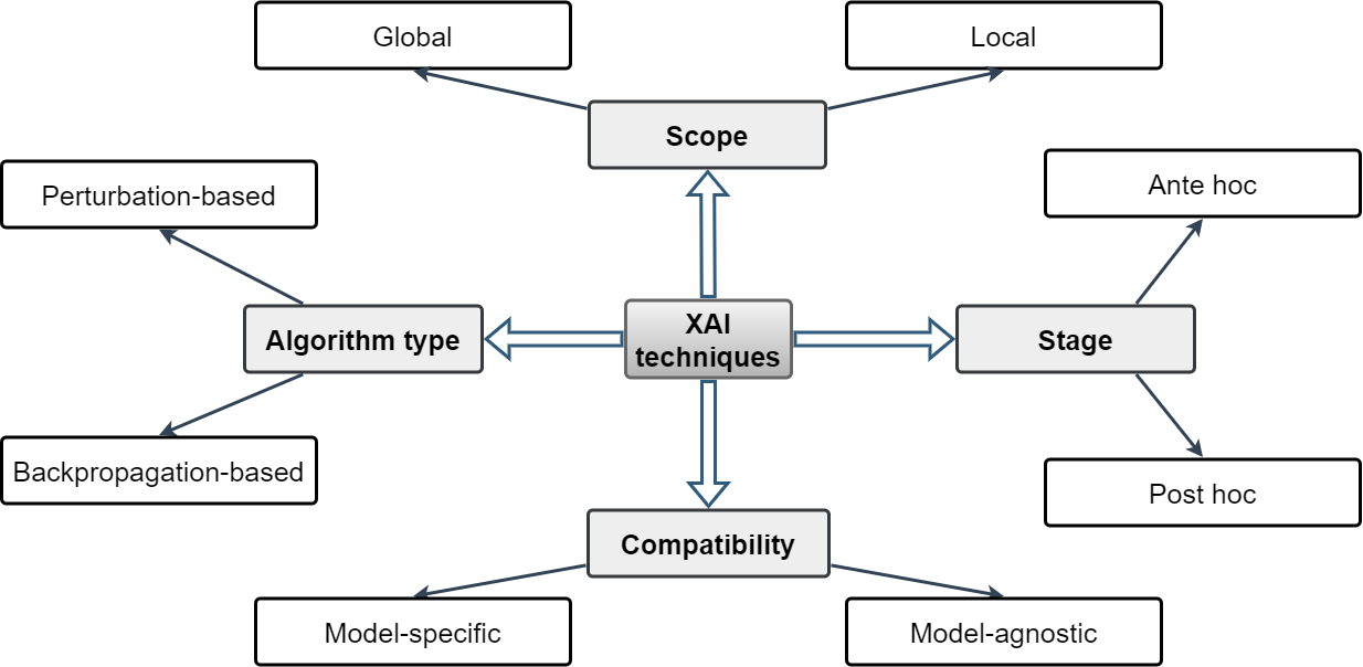
Figure 1: Summary of XAI techniques’ taxonomy based on their characteristics

2.3.2 Gradient-Weighted Class Activation Mapping (Grad-CAM)

Grad-CAM [29] is a more compatible version of CAM [40] that can be applied to any CNN model without the need to replace the stack of fully connected layers with a GAP layer. Thus, Grad-CAM is a local, backpropagation-based, post hoc, and model-specific XAI method.

In this method, we utilize the gradients of any target concept (say, logits for any class of interest) flowing through the final convolutional layer to generate a coarse localization map emphasizing the relevant portions of the image for predicting that concept. In other words, first, the gradient of logits $y$ of the class $c$ with respect to feature maps $A^{k}$ of a convolutional layer is computed. The gradients are then averaged across each feature map to calculate neuronal importance weights $\alpha_{k}^{c}$:

$$\alpha_{k}^{c}=\frac{1}{Z}\sum_{i}\sum_{j}\frac{\partial y^{c}}{\partial A_{ij}^{k}}.$$ (5)

This weight $\alpha_{k}^{c}$ captures the importance of the feature map $k$ for the target class $c$. Finally, we multiply each activation map by its importance score and sum the values. If we want to just consider the pixels with positive influence on the prediction of the class of interest, a ReLU is also applied to the summation:

$$L_{Grad-CAM}^{c}=ReLU(\sum_{k}\alpha_{k}^{c}A^{k}).$$ (6)

2.3.3 Local Interpretable Model-Agnostic Explanations (LIME)

LIME is an explanation technique that learns an interpretable model locally around the model’s prediction [27]. LIME is a local, perturbation-based, post hoc, and model-agnostic XAI method. In this approach, we want to minimize the following:

$$\xi(x)=\operatorname*{arg\,min}_{g\in G}\mathcal{L}(f,g,\pi_{x})+\Omega(g).$$ (7)

where $g\in G$ is an explanation model, which is in a class of potentially interpretable models $G$. $f$ is the original model, which we want to explain, and $\pi_{x}$ is a locality around $x$. $\Omega(g)$ is a measure of the complexity of the explanation $g$. Finally, $\mathcal{L}(f,g,\pi_{x})$ is a measure of how unfaithful $g$ is in approximating $f$ in the locality defined by $\pi_{x}$. To get an explanation for a single instance of interest using LIME, we perturb input features, obtain the model’s predictions for the new points, and then weight the new samples based on their closeness to the instance of interest. On the dataset containing the variations, we next train a weighted and interpretable model. Therefore, the prediction of an instance of interest may be explained by understanding the local model.

3 Related works

3.1 XAI for image classification

As our research focuses on explaining scene classification models, we only mention papers that use saliency-based XAI methods to explain an image classification model (or other tasks in which their inputs are images) in their work. A saliency map is a matrix whose size is the same as the model’s input image. Each element is assigned a distinct value (representation of color or intensity in images) based on its importance and relevance in generating the model’s prediction. LIME and GradCAM are two examples of saliency-based XAI techniques that were mentioned in section 2.3. In the following, we also discuss prior studies that presented various saliency-based XAI algorithms.

LRP, a model-specific post hoc XAI approach, was introduced in [28]. LRP explains a classifier’s prediction for a particular data point by assigning relevance scores to relevant input elements using the topology of the learned model. The authors of  [41], proposed AADN, a model-specific post hoc local explainer that can be applied only to differentiable models. It computes the gradients of the model’s prediction output based on its input features. DeepLIFT [42] is another model-specific, data-agnostic, post hoc XAI approach. It computes saliency maps backward, similar to LRP, but uses a baseline reference, similar to AADN. Instead of gradients, DeepLIFT utilizes the slope to explain how the output varies as the input deviates from a baseline. Authors in [43] used Shapley values (a game theory concept) to determine the significance of the model’s input features. SHAP is a model-agnostic explanation with two distinct explanators that may be utilized for image classification-specific deep neural networks: Deep-SHAP and Grad-SHAP. Deep-SHAP is a comparable approximation method to DeepLIFT. However, Grad-SHAP is based on IntegGRAD [41] and SmoothGRAD [44].

3.2 Image captioning

Our research is similar to some extent to the image captioning task, which takes an image as input and generates textual narratives that describe the image at hand in an encoder-decoder fashion [45]. Many research efforts have been put into developing an image captioning system capable of explaining visual data descriptively in a text-based format [46, 47, 48].

Unlike these approaches that provide a descriptive text by utilizing the encoded feature representation from the image, we generate a caption that explains the reasoning behind the scene classification by indicating the objects that contribute to the prediction. Furthermore, we do not perform text generation via an encoder-decoder structure, instead, we employ a novel module to apply logical instructions and functions to provide captioning text.

3.3 Scene classification

Our work can be considered most related to the following studies in terms of using environmental objects as important components to improve scene classification. Chen et al. [49] considered the objects as the context in the scene and proposed to derive object embeddings by implementing an object segmentation module, and leveraged these vectors to refine the top-5 predictions of ResNet [5] to improve scene recognition. On the other hand, Heikel et al. [50] used YOLO as an object detection architecture to extract objects from the scene. They further mapped these objects to TF-IDF feature vectors and utilized them for training a scene classifier to predict scene categories. As for the explainability aspect of scene classification, the work of Anjomshoae et al. [51] is the most related to our approach in providing text-based explanations by using local information (i.e., objects). It generated textual explanations by calculating the contextual importance of each semantic category in the scene by masking that particular segment, and determining its effect on the prediction. In contrast to these methods, our framework doesn’t solely rely on the scene objects to classify images; instead, it uses their information as a modifier to correct the output of the scene classification module when its softmax score doesn’t exceed a certain threshold.

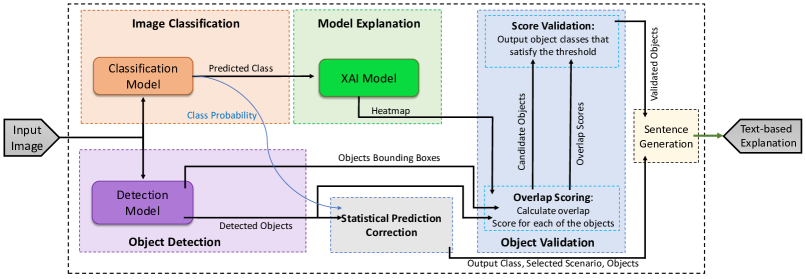
Figure 2: An overview of the proposed framework. The input image is first passed into both the object detection and image classification modules. Depending on the confidence of the prediction, the statistical prediction correction (SPC) decides the scenario of the system and determines the class of the input if the scene classifier’s prediction is not reliable (i.e., the class probability doesn’t satisfy a specific threshold). In the object validation module, the validated objects are obtained based on their overlap score calculated by the model explanation heatmap. Finally, based on the output class, selected scenario, validated objects, and all objects in the input image, the sentence generation module generates an appropriate sentence explaining the model.

4 The proposed method

The framework of our system is depicted in Figure 2. To promote a better understanding of the reasoning behind the prediction process, we propose a novel framework for interpretability by adopting previously developed explainability methods for deep learning models. Our TbExplain framework includes six major modules: (1) Image Classification, (2) Object Detection, (3) Model Explanation, (4) Object Validation, (5) Statistical Prediction Correction, and (6) Sentence Generation. The first step is to pass the input image to the Image classification and Object detection modules, which determine the category of the image and produce the proposals of the detected objects in the input, respectively. The output of the Image Classification module (the predicted class of the image) is then passed to the Model Explanation module to produce interpretable heatmaps capable of explaining the classification reasoning to a certain extent. Next, the heatmaps and object proposals are concurrently passed to the Object Validation module to quantify the overlap percentage of the object proposals with respect to the heatmaps. The Object Validation outputs to the Sentence Generation module the classes of objects whose percentage exceeds a predetermined threshold and are considered validated objects.

We also devised a statistical prediction correction method to increase generalization by incorporating a confidence measure to logically determine whether the output of the image classification module is reliable or not. Depending on how reliable the output of the image classification module is and what objects are in the image, one of three scenarios will be chosen as the selected scenario. If the output of the image classification module is reliable, the first scenario will be chosen; if it is not reliable and the object detection module detects some objects in the input image, the second scenario will be chosen; and if no objects were detected in the image, the third scenario will be chosen. In addition, when the output of Image Classification module is not reliable, SPC method makes a new prediction based on thg objects in the image. As a result, the selected scenario, objects in the image, and output class are outputs of this module passed to the Sentence Generation module. Finally, the Sentence Generation module generates an explanation based on the selected scenario. Following is a concise description of each of the six modules that make up the framework.

4.1 Image classification

The Image Classification module receives the input image and aims to predict its class among the predefined class memberships. The network’s output is a vector of probabilities, such that each index c corresponds to the probability of the input belonging to class c. The class with the highest probability is considered the prediction of the Image Classification. The produced probability distribution and the predicted class are further passed to the Model Explanation and SPC modules.

4.2 Object detection

The Object Detection module outputs the object classes and their corresponding bounding box coordinates detected in the input image. It outputs the objects that their detection confidence $DC$ (the confidence score of the object detection in detecting the object) is greater than a confidence threshold denoted as $T_{C}$. These contextual information are then passed to the Object Validation and SPC modules to help provide textual explanations and improve classification performance in a statistical manner.

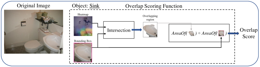
Figure 3: The structure of the overlap scoring function. The heatmap and the object bounding box ($b$) are passed through an intersection function to obtain the overlapping region ($OR$). The overlapping score is then calculated by dividing the area of $OR$ by $b$, which also plays the role of a normalization operation.

4.3 Model explanation

In this module, a XAI technique is used to interpret the scene classification model’s reasoning for predicting the output based on each input feature. The input image and the predicted class generated by the scene classification model are the inputs of the Model Explanation module. These inputs are given to the XAI model, which then generates a heatmap indicating the pixel relevance scores of each input to the prediction.

4.4 Object validation

To determine which objects contribute to the generation of the output of the image classification model, we propose a novel technique to detect these objects in the image by assessing a percentage called the Overlapping Score ($OS$). An overlapping score for each object reflects the percentage of the bounding box covered by the overall heatmap (the extracted regions from the original image that correspond to the heatmap areas). For example, a score of $OS=100$ indicates that the heatmap spans over the whole bounding box, and a score of 0 means that the bounding box is localized in a place where it has no intersection with the heatmap. Given the generated heatmap (X), as well as the set of detected bounding boxes (B), the process of determining the classes $\{c_{1},c_{2},…,c_{i}\}$ that exceed a certain threshold can be formulated as:

$$\{c_{1},c_{2},…,c_{i}\}=OV(X,B)$$ (8)

where $OV(.)$ represents the Object Validation module. As depicted in Figure 3, the overlapping region between the heatmap and the bounding box of the object i is obtained through an intersection operation. The overlap score is then calculated by dividing the area of the overlapped region by the area of the corresponding object bounding box. The whole operation can be defined as follows:

$$OS_{i}=\frac{Intersection(X,b_{i})}{b_{i}}$$ (9)

where $OS_{i}$ is the overlap score of the object i, and $b_{i}$ is the bounding box of the object i. The object classes $\{c_{1},c_{2},…,c_{i}\}$ that make significant contributions to the scene classification process are obtained via the score validation function. Additionally, the detection confidence of the objects $DC_{i}$ will be multiplied by $OS_{i}$ to obtain a relevence score $RS_{i}$. Finally, if $RS_{i}$ exceeds a relevance threshold $T_{R}$ for the corresponding object $i$, the class of the object $c_{i}$ will be output by the module as the validated object. A high relevence score indicates that not only is the object detected correctly, but it also contributes significantly to the classification.

4.5 Statistical prediction correction

Statistical Prediction Correction (SPC) is a logic-based decision maker conditioned on a confidence threshold, the softmax probability of the output class, to determine if the revision of the scene classification prediction is required and its procedure should be executed. SPC statistically learns $N_{c}$ (number of classes) weights for each object in the training phase by incrementally calculating the probability of the object occurring in each class:

$$W_{ic}=\frac{d_{ic}}{D_{i}}$$ (10)

Where $W_{ic}$ is denoted as the corresponding weight of an object i for class c, $d_{ic}$ as the number of times the object i has occurred in scenes belonging to class c, and $D_{i}$ as the quantification of the object i occurring in every scene from the dataset. It is important to note that these weight assessments are intended for the objects validated by the Object Validation module. In the test phase, if the scene classification model’s prediction can’t be regarded as reliable, the prediction is entrusted to the SPC, which leverages the estimated weights to decide the category of the input via calculating a weighted score for each of the classes in the following manner:

$$s_{1}=n_{1}W_{11}+n_{2}W_{21}+\cdots+n_{i}W_{i1}$$

$$s_{2}=n_{1}W_{12}+n_{2}W_{22}+\cdots+n_{i}W_{i2}$$

$$\bullet$$

$$\bullet$$ (11)

$$\bullet$$

$$s_{c}=n_{1}W_{1c}+n_{2}W_{2c}+\cdots+n_{i}W_{ic}$$

where $n_{i}$ indicates the quantity of object i existing in the scene. In contrast to the training phase, every object’s weight is incorporated to obtain the weighted score since the heatmap produced by the XAI technique is not accurate. Next, the class with the highest score s wins as the label of the input. We followed the following considerations to determine whether the scene classifier is justified in making the final decision for labeling the input (we indicate each situation as a scenario):

1. If the softmax output for the most probable class is higher than the confidence threshold, the output of image classification model is reliable enough to be assigned as the label, and validated objects will be used for generating a suitable explanation.

2. If the class probability is less than the confidence threshold, the label is decided by the SPC by selecting the class with the highest weighted score, and all detected objects in the image will be used to generate an acceptable explanation.

3. Occasionally, in spite of the class probability being less than the confidence threshold, the object detector recognizes no objects in the scene. As a result, the statistically weighted score for all the classes is zero, so inevitably, only the original scene classifier is capable of categorizing the input data, and there is no specific explanation in this case.

An illustration for each of the aforementioned cases is provided in Figure 4. The textual explanation is provided in a constant format, with only the predicted class and the intended objects changing with respect to the input.

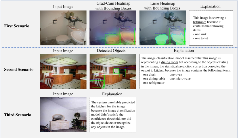
Figure 4: Outputs of TbExplain in three distinct scenarios. Each row is composed of the visual contents along with the text-based explanation relevant to the corresponding scenario.

4.5.1 The first scenario

The first scenario occurs when the probability value obtained for the predicted class is higher than a specific threshold, indicating that the model has made its prediction with enough confidence. When this happens, the input image and the classification model are fed into the proposed method to generate a text-based explanation, as demonstrated in Figure 4. In this scenario, the textual explanation is provided by representing the objects that contributed most to the model’s classification, and the output phrase confirms the class of the input by referring to these validated objects as the reason for the process.

4.5.2 The second scenario

The second scenario occurs when the probability value is below a predetermined threshold, indicating an unreliable prediction by the scene classification model. In this case, the SPC corrects the output class by generating a revised label based on the objects present in the input image. As a result, this approach outputs items that are relevant to the new predicted label. Figure 4 visually illustrates the output generated by the SPC approach in the second scenario.

4.5.3 The third scenario

The third scenario arises when the image classification model’s probability value for the top class falls below a predetermined threshold and the object detection module fails to detect any objects in the input image. In such cases, the interpretation highlights the unreliability of the system in making accurate predictions and displays the output of the image classification model. Moreover, the SPC module is unable to correct the unreliable predictions generated by the scene classification model. The output of TbExplain in this scenario is depicted in Figure 4 and suggests that the model may require further refinement and diagnosis.

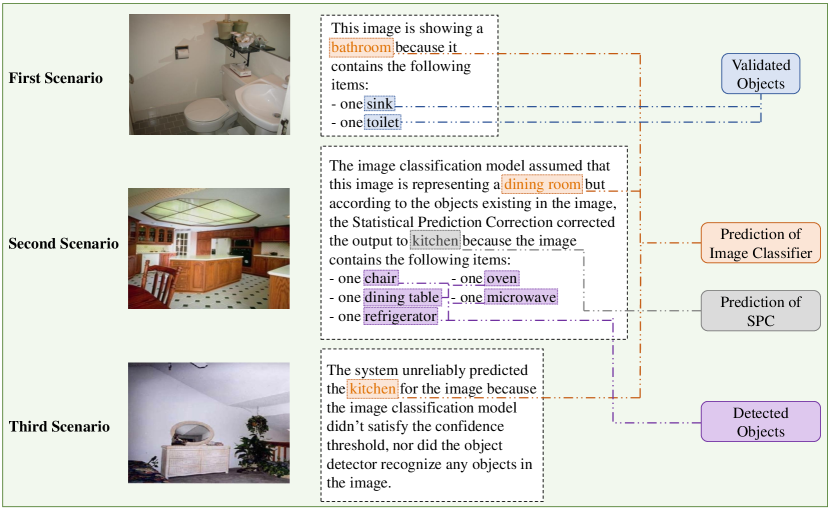
Figure 5: Examples of the sentence generation’s outputs (i.e., the text-based explanation). The highlights in the text indicate the components, including important objects and the prediction, that the designed modules provide for explaining the classification. The colors of the highlights distinguish the modules that assist the explanation in each scenario.

4.6 Sentence generation

To output the desired textual explanation, we implemented Sentence Generation to leverage the information provided by both SPC and the object validation modules and integrate them to set up the explanatory sentence. The procedure of the sentence generation can be interpreted as a fill-in-the-blank task. In each scenario, a fixed sentence with several missing words that are either the prediction or the pertaining objects is the general structure of the explanation. As illustrated in Figure 5, the objective is to provide this missing information by utilizing the scene classification’s prediction in all scenarios, the validated objects in the first scenario, the revised prediction of the SPC module and all detected objects in the second scenario.

5 Experiments

5.1 Datasets and pre-processing

Table 1: A summary of the details of the datasets that we select for conducting our experiments.

Dataset	Total number of images	Number of categories	Number of images per category
MIT67	15,620	67	100+
Places365 (standard version)	2,000,000+	400+	3,068 - 5,000
SUN397	108,753	397	100+

We selected three datasets to evaluate the performance of TbExplain. In Table 1, a summary of their details can be observed, and a brief description is provided as follows:

• First, we select the MIT67 dataset [52], which comprises 67 indoor categories and 15,620 images in total. The quantity of images varies according to the category, and each one contains at least 100 images.

• Additionally, we select the Places365 dataset [53], which contains more than 2 million images comprising more than 400 scene categories. This dataset contains between 3,068 and 5,000 training images per category.

• Finally, we select the SUN397 dataset [54], which contains 108,753 images of 397 scene categories. Same as in the MIT67 dataset, the number of images varies across categories in the SUN397 dataset too, but there are at least 100 images per category.

Due to the vast size of the dataset, the hardware limitations for processing these data, and the considerable similarity of a number of classes to one another, only 9 categories out of all categories were selected for each dataset, followed by the selection of all images labeled with one of these 9 classes. In Table 2, the selected categories are specified separately for each dataset. We selected and extracted different categories for each dataset because, by doing this, we can reliably make sure of the efficiency and functionality of the model proposed in this paper. This selection strategy ensures that the model works for any class of scene category.

We randomly selected 78 images per chosen category from the MIT67 dataset and 75 images for the other two datasets as training data. These new datasets, derived from the original ones and each with nine categories, were selected as our experimental data. To generate test data for each dataset, we randomly selected 25 images for each of the nine classes. We also randomly selected 10% of the training data as validation data. Finally, we convert all image sizes to $256\times 256$ pixel and normalize all pixel values from $[0,255]\in\mathbb{N}$ to $[0,1]\in\mathbb{R}$.

5.2 Implementation protocol

We utilized various versions of pre-trained ResNet on the ImageNet dataset [14] and a pre-trained YOLOv5 on the COCO dataset [55] as the scene classification and object detection models, respectively. We also employed GradCAM and LIME as internal XAI techniques in the Model Explanation module. The computational resources for this study are a 12GB of RAM and a Nvidia Tesla K80 GPU.

Table 2: List of selected categories per dataset in the data pre-processing phase. We fine-tune, validate, and test scene classification models and TbExplain in these categories.

Dataset	Title of selected categories
MIT67	auditorium - bakery - bar - bathroom - bedroom bookstore - dining room - florist - kitchen
Places365 (standard version)	baseball field - boat deck - classroom - galley - garage indoor highway - living room - television room - vegetable garden
SUN397	art studio - computer room - street - restaurant - supermarket restaurant kitchen - waiting room - wine cellar - bottle storage - train railway

5.3 Qualitative analysis

In this section, we evaluate the reliability of TbExplain’s textual explanations by comparing its results with the manually annotated data. In detail, 108 scene images from 9 different classes (12 images from each class) were randomly divided among the three authors of this paper to manually annotate them. In fact, each author should look at each scene and identify and record three of the most relevant and important objects in the scene that are representative of that class (e.g., the "bed" object is a representative of the "bedroom" class). If less than three representative objects were recognizable in the image, the author should fill the empty slots with "empty".

Finally, we compare the identified objects with the objects presented in the TbExplain textual explanation for each scene. We obtained 65.94% accuracy in this experiment. It means that in 65.94% of cases, our method reliably and correctly interprets the reasoning involved in scene classification by presenting the most relevant objects within the scene (as representative objects of that class) in its textual explanation. Therefore, by reading the proposed explanation of the model’s functionality, non-expert users can readily understand the underlying reasoning of the model.

5.4 Quantitative analysis

In this section, we quantitatively evaluate the effectiveness of TbExplain (in the second scenario using the SPC method) by comparing its performance with the original image classification model’s accuracy.

For tuning the proposed method’s performance, we should adjust three hyperparameters:

1. Confidence threshold ($T_{C}$), which specifies in the object detection module whether a detected object is a valid object or not.

2. Relevance threshold ($T_{R}$), which specifies whether a valid object is a relevant object according to the predicted class or not.

3. Class Probability threshold ($T_{P}$) which is a threshold on the probability value of the top class in the last layer of the scene classification model that specifies the scenarios mentioned in the previous section. In fact, $T_{P}$ is a threshold on the model’s prediction confidence.

Table 3: A comparison between the achieved accuracy of TbExplain and four versions of ResNet on the MIT67 dataset. TbExplain with Lime and ResNet101V2 as the XAI technique and scene classification model, respectively, yields the best results (82.47% accuracy).

Method	Training Accuracy	Validation Accuracy	Testing Accuracy
ResNet50	99.96%	71.07%	70.31%
ResNet50V2	99.92%	75.35%	75.67%
ResNet101	99.96%	71.78%	68.3%
ResNet101V2	99.96%	79.28%	78.34%
TbExplain (LIME)	-	-	82.47%
TbExplain (GradCAM)	-	-	82.25%

We employed grid-search with 4-fold cross-validation on the MIT67 dataset and validated TbExplain to assess the best values of the thresholds based on the validation data. The grid-search procedure is performed using the following parameters: values of $\{0.2,0.4,0.6,0.8\}$ for $T_{C}$, values of $\{0.2T_{C},0.4T_{C},0.6T_{C},\\ 0.8T_{C}\}$ for $T_{R}$, and 10 distinct values for $T_{P}$, from $0.1$ to $1$ with a step size of $0.1$.

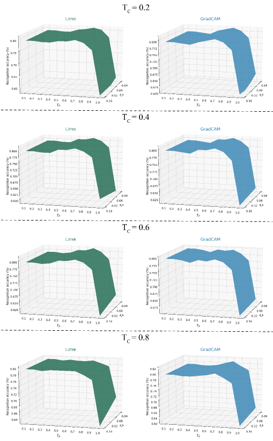
Figure 6: Recognition accuracy of TbExplain on the validation set based on the specified thresholds $T_{C}$, $T_{R}$, and $T_{P}$.

Table 4: A comparison between the achieved accuracy of TbExplain and four versions of ResNet on the Places365 (standard version) dataset. TbExplain with LIME and ResNet101V2 as the XAI technique and scene classification model, respectively, yields the best results (78.22% accuracy).

Method	Training Accuracy	Validation Accuracy	Testing Accuracy
ResNet50	100%	71.64%	68.44%
ResNet50V2	100%	77.61%	74.22%
ResNet101	100%	70.14%	68.44%
ResNet101V2	100%	79.10%	75.55%
TbExplain (LIME)	-	-	78.22%
TbExplain (GradCAM)	-	-	77.33%

Table 5: A comparison between the achieved accuracy of TbExplain and four versions of ResNet on the SUN397 dataset. TbExplain with LIME and ResNet101V2 as the XAI technique and scene classification model, respectively, yields the best results (80% accuracy).

Method	Training Accuracy	Validation Accuracy	Testing Accuracy
ResNet50	100%	73.13%	63.11%
ResNet50V2	100%	74.62%	68.88%
ResNet101	100%	67.16%	65.33%
ResNet101V2	100%	79.10%	79.11%
TbExplain (LIME)	-	-	80%
TbExplain (GradCAM)	-	-	79.55%

Figure 6 demonstrates grid-search results on the validation data with $T_{C}$, $T_{R}$, and $T_{P}$ as the parameters. The best performance is achieved with $T_{C}=0.2,T_{R}=0.08$, and $T_{P}=0.7$. The comparison of TbExplain on the test set with various variations of ResNet represents an improvement in terms of prediction accuracy, with Lime-integrated TbExplain achieving 82.47% accuracy (4.13% higher than the best variation of ResNet). In other words, the SPC method corrects 4.13% of the original classification model’s false predictions. Table 3 summaries the achieved performance of four versions of ResNet and TbExplain (in the second scenario using SPC method) on MIT67.

It should be noted that since the XAI methods are applied to the original scene classification model and cannot independently report the classification accuracy, TbExplain is actually the output of applying the proposed second scenario to the pre-trained ResNet101V2 to improve its performance. Therefore, there is no need for training and validation again, and for this reason, the accuracy value for training and validation of TbExplain is not reported in the above-mentioned table.

As mentioned in section 5.1, we also retrained all versions of ResNet on two other datasets (Places365 and SUN397) and tested TbExplain on them, utilizing the learned threshold values ($T_{C}=0.2,T_{R}=0.08$, and $T_{P}=0.7$) to ensure TbExplain’s robustness and generalizability in different scenes and environments. Since generalizing to scenes and images with different contextual information, such as different objects and backgrounds, is of high significance, we chose environments that were dissimilar to MIT67 from SUN397 and Places365. Table 4 and Table 5 summarize the performance achieved by all the above-mentioned versions of ResNet and TbExplain on the Places365 and SUN397 datasets, respectively. According to these two tables, the effectiveness of our model in increasing the classification accuracy can be seen on other datasets as well.

Figure 7 provides a summary of the performance of TbExplain and the best performing ReNet model on all three datasets.

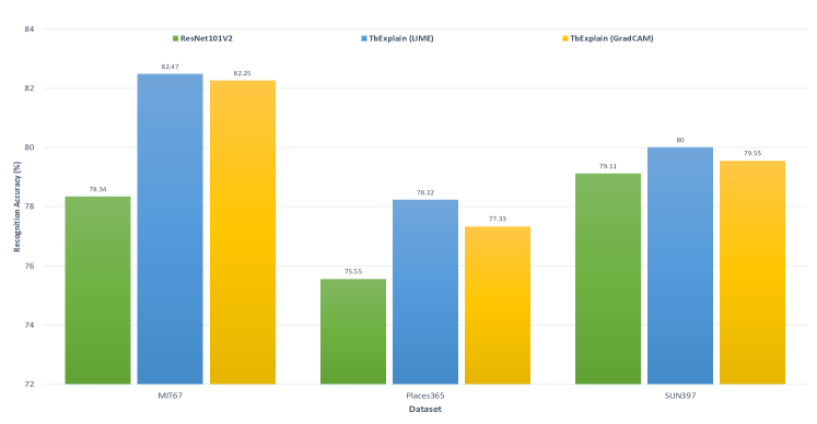
Figure 7: A summary of the performance of TbExplain and ResNet101V2 on all three datasets.

To further examine the performance of TbExplain, we present in Figure 8 the confusion matrices generated using $T_{C}=0.2,T_{R}=0.08$, and $T_{P}=0.7$ as the threshold values, with the true labels on the y-axis and the predicted labels on the x-axis.

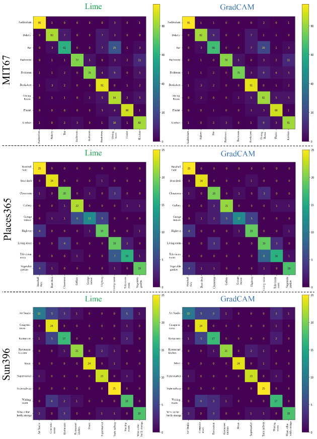
Figure 8: The confusion matrices generated for the three scene datasets utilizing TbExplain with Lime and GradCAM.

6 Limitations and future work

Our work contains several limitations and suggests research opportunities that can be addressed in future work to advance the field. Firstly, a comparative study can be performed with other explainability algorithms for better analysis and evaluation. Secondly, the object detection model (YOLOv5 in our case) is pretrained on a dataset different from the data adopted in our study, so it can be fine-tuned and adapted to further improve the robustness and performance of object detection and the overall system. Lastly, since the provided explanation in a static format hinders flexibility, future works can include methods to produce these sentences in a creative and versatile manner.

7 Conclusion

In this paper, we propose a novel framework, called TbExplain, that generates text-based explanations for scene classification models. The text-based explanations consist of a sentence that attempts to explain the reasoning behind the prediction by indicating the scene objects that contribute to the classification process. We further attempted to improve classification accuracy by devising a statistical-based approach, called Statistical Prediction Correction (SPC), to correct the prediction by incorporating the confidence of the prediction and scene objects.  In our experiments, we utilized ResNet101V2 and YOLOv5 as the scene classification and object detection models, respectively, and also employed GradCAM and LIME as internal XAI techniques in our framework. In the qualitative analysis, we evaluate the reliability and trustworthiness of TbExplain’s text-based explanations by comparing them with the manually annotated data labels. Furthermore, the quantitative analysis conducted on the MIT67, SUN397, and Places365 datasets confirmed the efficacy of our proposed framework in improving classification performance. In fact, in this experiment, we apply TbExplain to a pre-trained scene classification model, which increases the classification accuracy in light of our proposed SPC method.

Declaration of competing interest

The authors declare that they have no known competing financial interests or personal relationships that could have appeared to influence the work reported in this paper.

Data availability

All the data used in this work is from open and publicly available datasets for scene classification.

References

- [1] V. H. Pereira-Ferrero, L. P. Valem, D. C. G. Pedronette, Feature augmentation based on manifold ranking and lstm for image classification, Expert Systems with Applications 213 (2023) 118995.
- [2] D. R. Bruno, F. S. Osorio, Image classification system based on deep learning applied to the recognition of traffic signs for intelligent robotic vehicle navigation purposes, in: 2017 Latin American Robotics Symposium (LARS) and 2017 Brazilian Symposium on Robotics (SBR), IEEE, 2017, pp. 1–6.
- [3] P. Deepan, L. Sudha, Object classification of remote sensing image using deep convolutional neural network, in: The cognitive approach in cloud computing and internet of things technologies for surveillance tracking systems, Elsevier, 2020, pp. 107–120.
- [4] H. Barzekar, Z. Yu, C-net: A reliable convolutional neural network for biomedical image classification, Expert Systems with Applications 187 (2022) 116003.
- [5] K. He, X. Zhang, S. Ren, J. Sun, Deep residual learning for image recognition, in: Proceedings of the IEEE conference on computer vision and pattern recognition, 2016, pp. 770–778.
- [6] K. He, X. Zhang, S. Ren, J. Sun, Delving deep into rectifiers: Surpassing human-level performance on imagenet classification, in: Proceedings of the IEEE international conference on computer vision, 2015, pp. 1026–1034.
- [7] M.-H. Horng, Multi-class support vector machine for classification of the ultrasonic images of supraspinatus, Expert Systems with Applications 36 (4) (2009) 8124–8133.
- [8] Y. Lai, A comparison of traditional machine learning and deep learning in image recognition, in: Journal of Physics: Conference Series, Vol. 1314, IOP Publishing, 2019, p. 012148.
- [9] Y. LeCun, Y. Bengio, G. Hinton, Deep learning, nature 521 (7553) (2015) 436–444.
- [10] S. Bai, Growing random forest on deep convolutional neural networks for scene categorization, Expert systems with applications 71 (2017) 279–287.
- [11] P. S. Yee, K. M. Lim, C. P. Lee, Deepscene: Scene classification via convolutional neural network with spatial pyramid pooling, Expert Systems with Applications 193 (2022) 116382.
- [12] M. D. Ferreira, D. C. Corrêa, L. G. Nonato, R. F. de Mello, Designing architectures of convolutional neural networks to solve practical problems, Expert Systems with Applications 94 (2018) 205–217.
- [13] J. Chai, H. Zeng, A. Li, E. W. Ngai, Deep learning in computer vision: A critical review of emerging techniques and application scenarios, Machine Learning with Applications 6 (2021) 100134.
- [14] O. Russakovsky, J. Deng, H. Su, J. Krause, S. Satheesh, S. Ma, Z. Huang, A. Karpathy, A. Khosla, M. Bernstein, et al., Imagenet large scale visual recognition challenge, International journal of computer vision 115 (3) (2015) 211–252.
- [15] K. Simonyan, A. Zisserman, Very deep convolutional networks for large-scale image recognition, arXiv preprint arXiv:1409.1556 (2014).
- [16] C. Szegedy, W. Liu, Y. Jia, P. Sermanet, S. Reed, D. Anguelov, D. Erhan, V. Vanhoucke, A. Rabinovich, Going deeper with convolutions, in: Proceedings of the IEEE conference on computer vision and pattern recognition, 2015, pp. 1–9.
- [17] F. Doshi-Velez, B. Kim, Towards a rigorous science of interpretable machine learning, arXiv preprint arXiv:1702.08608 (2017).
- [18] F. Cabitza, A. Campagner, G. Malgieri, C. Natali, D. Schneeberger, K. Stoeger, A. Holzinger, Quod erat demonstrandum?-towards a typology of the concept of explanation for the design of explainable ai, Expert Systems with Applications 213 (2023) 118888.
- [19] D. V. Carvalho, E. M. Pereira, J. S. Cardoso, Machine learning interpretability: A survey on methods and metrics, Electronics 8 (8) (2019) 832.
- [20] D. Wang, Q. Yang, A. Abdul, B. Y. Lim, Designing theory-driven user-centric explainable ai, in: Proceedings of the 2019 CHI conference on human factors in computing systems, 2019, pp. 1–15.
- [21] T. Kulesza, M. Burnett, W.-K. Wong, S. Stumpf, Principles of explanatory debugging to personalize interactive machine learning, in: Proceedings of the 20th international conference on intelligent user interfaces, 2015, pp. 126–137.
- [22] L. H. Gilpin, D. Bau, B. Z. Yuan, A. Bajwa, M. Specter, L. Kagal, Explaining explanations: An overview of interpretability of machine learning, in: 2018 IEEE 5th International Conference on data science and advanced analytics (DSAA), IEEE, 2018, pp. 80–89.
- [23] R. Agarwal, L. Melnick, N. Frosst, X. Zhang, B. Lengerich, R. Caruana, G. E. Hinton, Neural additive models: Interpretable machine learning with neural nets, Advances in Neural Information Processing Systems 34 (2021) 4699–4711.
- [24] C. Barberan, S. Alemmohammad, N. Liu, R. Balestriero, R. Baraniuk, Neuroview-rnn: It’s about time, in: 2022 ACM Conference on Fairness, Accountability, and Transparency, 2022, pp. 1683–1697.
- [25] L.-T. Huang, M. M. Gromiha, S.-Y. Ho, iptree-stab: interpretable decision tree based method for predicting protein stability changes upon mutations, Bioinformatics 23 (10) (2007) 1292–1293.
- [26] Q. Zhang, Y. N. Wu, S.-C. Zhu, Interpretable convolutional neural networks, in: Proceedings of the IEEE conference on computer vision and pattern recognition, 2018, pp. 8827–8836.
- [27] M. T. Ribeiro, S. Singh, C. Guestrin, " why should i trust you?" explaining the predictions of any classifier, in: Proceedings of the 22nd ACM SIGKDD international conference on knowledge discovery and data mining, 2016, pp. 1135–1144.
- [28] S. Bach, A. Binder, G. Montavon, F. Klauschen, K.-R. Müller, W. Samek, On pixel-wise explanations for non-linear classifier decisions by layer-wise relevance propagation, PloS one 10 (7) (2015) e0130140.
- [29] R. R. Selvaraju, M. Cogswell, A. Das, R. Vedantam, D. Parikh, D. Batra, Grad-cam: Visual explanations from deep networks via gradient-based localization, in: Proceedings of the IEEE international conference on computer vision, 2017, pp. 618–626.
- [30] E. Cambria, L. Malandri, F. Mercorio, M. Mezzanzanica, N. Nobani, A survey on XAI and natural language explanations, Information Processing and Management 60 (103111) (2023).
- [31] E. Cambria, Q. Liu, S. Decherchi, F. Xing, , K. Kwok, SenticNet 7: A commonsense-based neurosymbolic AI framework for explainable sentiment analysis, in: LREC, 2022, pp. 3829–3839.
- [32] S. Han, R. Mao, E. Cambria, Hierarchical attention network for explainable depression detection on twitter aided by metaphor concept mappings, in: Proceedings of COLING, 2022, pp. 94–104.
- [33] M. Ge, R. Mao, E. Cambria, Explainable metaphor identification inspired by conceptual metaphor theory, in: Proceedings of the 36th AAAI Conference on Artificial Intelligence, 2022, pp. 10681–10689.
- [34] A. Kazemeini, S. S. Roy, R. E. Mercer, E. Cambria, Interpretable representation learning for personality detection, in: 2021 International Conference on Data Mining Workshops (ICDMW), IEEE, 2021, pp. 158–165.
- [35] K. Simonyan, A. Vedaldi, A. Zisserman, Deep inside convolutional networks: Visualising image classification models and saliency maps, arXiv preprint arXiv:1312.6034 (2013).
-
[36]
G. Jocher, A. Stoken, J. Borovec, NanoCode012, A. Chaurasia, TaoXie,
L. Changyu, A. V, Laughing, tkianai, yxNONG, A. Hogan, lorenzomammana,
AlexWang1900, J. Hajek, L. Diaconu, Marc, Y. Kwon, oleg, wanghaoyang0106,
Y. Defretin, A. Lohia, ml5ah, B. Milanko, B. Fineran, D. Khromov, D. Yiwei,
Doug, Durgesh, F. Ingham,
ultralytics/yolov5: v5.0 -
YOLOv5-P6 1280 models, AWS, Supervise.ly and YouTube integrations (Apr.
2021).
doi:10.5281/zenodo.4679653.
URL https://doi.org/10.5281/zenodo.4679653 - [37] J. Redmon, S. Divvala, R. Girshick, A. Farhadi, You only look once: Unified, real-time object detection, in: Proceedings of the IEEE conference on computer vision and pattern recognition, 2016, pp. 779–788.
- [38] S. Liu, L. Qi, H. Qin, J. Shi, J. Jia, Path aggregation network for instance segmentation, in: Proceedings of the IEEE conference on computer vision and pattern recognition, 2018, pp. 8759–8768.
- [39] K. He, X. Zhang, S. Ren, J. Sun, Identity mappings in deep residual networks, in: European conference on computer vision, Springer, 2016, pp. 630–645.
- [40] B. Zhou, A. Khosla, A. Lapedriza, A. Oliva, A. Torralba, Learning deep features for discriminative localization, in: Proceedings of the IEEE conference on computer vision and pattern recognition, 2016, pp. 2921–2929.
- [41] M. Sundararajan, A. Taly, Q. Yan, Axiomatic attribution for deep networks, in: International conference on machine learning, PMLR, 2017, pp. 3319–3328.
- [42] A. Shrikumar, P. Greenside, A. Kundaje, Learning important features through propagating activation differences, in: International conference on machine learning, PMLR, 2017, pp. 3145–3153.
- [43] S. M. Lundberg, S.-I. Lee, A unified approach to interpreting model predictions, Advances in neural information processing systems 30 (2017).
- [44] D. Smilkov, N. Thorat, B. Kim, F. Viégas, M. Wattenberg, Smoothgrad: removing noise by adding noise, arXiv preprint arXiv:1706.03825 (2017).
- [45] M. Stefanini, M. Cornia, L. Baraldi, S. Cascianelli, G. Fiameni, R. Cucchiara, From show to tell: a survey on deep learning-based image captioning, IEEE Transactions on Pattern Analysis and Machine Intelligence (2022).
- [46] O. Vinyals, A. Toshev, S. Bengio, D. Erhan, Show and tell: A neural image caption generator, in: Proceedings of the IEEE conference on computer vision and pattern recognition, 2015, pp. 3156–3164.
- [47] S. J. Rennie, E. Marcheret, Y. Mroueh, J. Ross, V. Goel, Self-critical sequence training for image captioning, in: Proceedings of the IEEE conference on computer vision and pattern recognition, 2017, pp. 7008–7024.
- [48] L. Huang, W. Wang, J. Chen, X.-Y. Wei, Attention on attention for image captioning, in: Proceedings of the IEEE/CVF international conference on computer vision, 2019, pp. 4634–4643.
- [49] B. X. Chen, R. Sahdev, D. Wu, X. Zhao, M. Papagelis, J. K. Tsotsos, Scene classification in indoor environments for robots using context based word embeddings, arXiv preprint arXiv:1908.06422 (2019).
- [50] E. Heikel, L. Espinosa-Leal, Indoor scene recognition via object detection and tf-idf, Journal of Imaging 8 (8) (2022) 209.
- [51] S. Anjomshoae, D. Omeiza, L. Jiang, Context-based image explanations for deep neural networks, Image and Vision Computing 116 (2021) 104310.
- [52] A. Quattoni, A. Torralba, Recognizing indoor scenes, in: 2009 IEEE conference on computer vision and pattern recognition, IEEE, 2009, pp. 413–420.
- [53] B. Zhou, A. Lapedriza, A. Khosla, A. Oliva, A. Torralba, Places: A 10 million image database for scene recognition, IEEE Transactions on Pattern Analysis and Machine Intelligence (2017).
- [54] J. Xiao, J. Hays, K. A. Ehinger, A. Oliva, A. Torralba, Sun database: Large-scale scene recognition from abbey to zoo, in: 2010 IEEE computer society conference on computer vision and pattern recognition, IEEE, 2010, pp. 3485–3492.
- [55] T.-Y. Lin, M. Maire, S. Belongie, J. Hays, P. Perona, D. Ramanan, P. Dollár, C. L. Zitnick, Microsoft coco: Common objects in context, in: Computer Vision–ECCV 2014: 13th European Conference, Zurich, Switzerland, September 6-12, 2014, Proceedings, Part V 13, Springer, 2014, pp. 740–755.