As large as it gets: Learning infinitely large Filters via Neural Implicit Functions
in the Fourier Domain

Abstract

Motivated by the recent trend towards the usage of larger receptive fields for more context-aware neural networks in vision applications, we aim to investigate how large these receptive fields really need to be. To facilitate such study, several challenges need to be addressed, most importantly: (i) We need to provide an effective way for models to learn large filters (potentially as large as the input data) without increasing their memory consumption during training or inference, (ii) the study of filter sizes has to be decoupled from other effects such as the network width or number of learnable parameters, and (iii) the employed convolution operation should be a plug-and-play module that can replace any conventional convolution in a Convolutional Neural Network (CNN) and allow for an efficient implementation in current frameworks. To facilitate such models, we propose to learn not spatial but frequency representations of filter weights as neural implicit functions, such that even infinitely large filters can be parameterized by only a few learnable weights. The resulting neural implicit frequency CNNs are the first models to achieve results on par with the state-of-the-art on large image classification benchmarks while executing convolutions solely in the frequency domain and can be employed within any CNN architecture. They allow us to provide an extensive analysis of the learned receptive fields. Interestingly, our analysis shows that, although the proposed networks could learn very large convolution kernels, the learned filters practically translate into well-localized and relatively small convolution kernels in the spatial domain.

1 Introduction

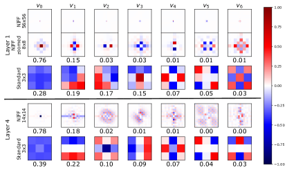
Figure 1: PCA components of learned kernel weights in the first layer of a ResNet50 trained on ImageNet100: 1st and 2nd rows shown large NIFF kernels in the spatial domain and a zoomed-in version with explained variance for each component (below). 3rd row: PCA and explained variance for a standard CNN with the standard kernel size 3x3. 4th and 5th row show that NIFF actually allows the model to learn large spatial filters for the 4th layer of the same network. PCA analysis is one of the tools we apply to answer the central question of this paper: How large do CNN kernels really need to be?

Inspired by the success of vision transformers for image classification tasks [12, 21, 48, 50], which rely on the learned self-attention between large image patches rather than small convolution kernels, and the development of Swin transformer [11, 24, 25] with shifted window attention of sizes ranging from $7\times 7$ to $12\times 12$, recent convolution-based vision models also return to leveraging large filters. A first example is the ConvNeXt architecture [26] with kernel sizes up to $7\times 7$, which started the trend to go towards using even larger receptive fields for vision tasks [16, 23, 26]. [10, 33] took kernel sizes to another level by increasing kernels to $31\times 31$ or even $51\times 51$ in order to further widen the receptive context. Our work presents an analysis of the kernel size for image classification tasks and is motivated by the practical question: How large do CNN kernels really need to be? Thus, we provide an extensive analysis of the learned receptive fields of CNNs which we enable to learn infinitely large kernels. To do so, we use a simple, yet effective trick: we compute the convolution in the frequency domain rather than in the spatial domain. However, the convolution in the spatial domain translates into an element-wise multiplication in the frequency domain. These element-wise multiplications do not translate directly in the common finite convolutions in the spatial domain, as they implement circular convolutions which are equivalent to the implementation of infinitly large kernels in the spatial domain. Moreover, point-wise multiplications are much more time and resource efficient than spatial convolutions with large kernels, yet the transformation between spatial and frequency domain remains a cost factor. The results of our empirical analysis show that although our network modification allows CNNs to learn infinite large filters, in practice the learned filters in the frequency domain transform into well-localized and relatively small convolutional kernels (up to 9x9 even tough 224x224 would be possible) in the spatial domain. Our contributions can be summarized as follows:

• We introduce a novel approach which enables CNNs to learn infinitely large convolutional filters that are only limited in their bandwidth and not by the size of their receptive field.

• To facilitate such models, we introduce MLP parameterized neural implicit frequency filters (NIFFs) which allow CNNs to learn filters directly in the frequency domain.

• We then analyse the spatial representations of the resulting large receptive fields learned by various CNN architectures on multiple datasets. While keeping most models’ performance on par with the baseline without any hyperparameter tuning.

• Hence, we are the first to introduce infinite frequency filters which can be plugged into any CNN architecture as a tool for analysing and understanding CNNs in depth.

2 Related Work

2.1 Large kernel sizes

Historically, only a few networks used large kernel sizes like AlexNet [22] or InceptionNets [43, 44, 45]. However, after the success of VGGNets [40] the focus shifted in the direction of small kernel sizes due to their computational efficiency and empirically better performances. Yet, in recent years, vision transformers facilitated a significant improvement in image classification tasks [12, 21, 48, 50]. Such models are based on larger image patches and self-attention, leading to the assumption that neural networks for image processing benefit from larger receptive fields. Especially [25] showed that larger receptive fields by shifted window attention, ranging from window sizes of $7\times 7$ to $12\times 12$, can boost the network’s performance. This shifted window attention can also be seen as large convolutional kernels and has been extended to larger sizes in follow-up work [11, 24]. Also, [26] showed that using larger kernels, with size $7\times 7$ could increase classification performance and even outperform transformer models. Further, [16, 33] increased the receptive fields of the convolutions even more and [10] up to $31\times 31$ as well as [23] up to $61\times 61$, providing a better context understanding, thus leading to better performance on classification, segmentation or object detection tasks. Yet, learning large kernels with many free parameters in an efficient way is non-trivial. Therefore, [10] use depthwise convolutions instead of full convolutions and argue that the increase in parameters would only be between 10 and 16%. [23] decompose the large $61\times 61$ into two parallel and rectangular convolutions to avoid computational overhead.
Besides the computational overhead, applying large kernels can also have further downsides as [47] showed that one needs to take precautions to reduce possible leakage artifacts. Thus, they propose to apply hamming windows. Further [35] propose Global Filter Networks which have a Swin-Transformer architecture and learn their convolutions in the frequency domain. However, they directly learn these filters resulting in a huge computational overhead additionally to the increased computational effort resulting from the Swin-Transformer architecture. Contrary to [35] our approach is designed to evaluate the effective filtersize of CNNs rather than Transformer. Moreover, our approach uses NIFF to reduce the computational overhead resulting from learning large kernel weights.

2.2 Training CNNs in the Frequency Domain

Most works implementing convolutions in the frequency domain focus on time and space efficiency of this operation [2, 15, 29, 34, 49, 52], since the equivalent for convolution in the spatial domain, is a point-wise multiplication in the frequency domain. However, most of these approaches still learn the convolution in the conventional setting in the spatial domain and transform the feature maps and kernels into the frequency domain to make use of the faster point-wise multiplication [2, 29, 52] at inference time. This is mostly due to the fact that one would practically need to learn filters as large as the feature maps when directly learning the frequency representation. Hence, previous approaches still learn small convolution kernels in the spatial domain and pad these kernels to the size of the feature map to make use of the efficiency of the element-wise multiplication.

Those few but notable works that also propose to learn convolutional filters in CNNs purely in the frequency domain, until now, could only achieve desirable evaluation performances on MNIST and reach low accuracies on more complex datasets like CIFAR or ImageNet [32, 34, 53] if they afford to evaluate on such benchmarks at all.

Further approaches apply model compression by zeroing out small coefficients of the feature map in the frequency domain [15] or enrich conventional convolutions which extract local information with the frequency perspective to get more global information [6].

In contrast to all these approaches we neither aim to be more time or space efficient nor do we want to boost performance via additional information. We aim to investigate how much of the receptive field CNNs practically make use of, if they have the opportunity to learn infinitely large kernels. Yet, to do so, we propose a model that facilitates learning large filters directly in the frequency domain via neural implicit functions. Thus, we are the first to propose a CNN whose convolutions can be fully learned in the frequency domain while maintaining state-of-the-art performance on common image classification benchmarks.

2.3 Neural Implicit Representations

Neural implicit representations generally map a location encoded by coordinates via an MLP to a continuous output domain. Thus, an object is represented by a function rather than fixed discrete values, which is commonly the case e.g. discrete grids of pixels for images, discrete samples of amplitudes for audio signals, and voxels, meshes or point clouds for 3D shapes [8, 41] or discrete kernel weights for point cloud convolutions [51]. Especially for 3D tasks like shape learning [7, 14, 31], modelling object shapes [1, 5, 38, 41] or surfaces for scenes [3, 9, 20, 42] this concept is widely used. Apart from the continuous representation of the signal, neural implicit representations have the advantage of having a fixed amount of parameters and being independent of spatial resolutions. Moreover, neural implicit representation can also be used to learn 2D images for generating high-resolution data [4], or learn 3D representations from 2D data. Particularly, in the currently popular field of Neural Radiance Fields (NeRF) [30, 54] neural implicit functions representations are broadly applied.

Further, [27, 28] introduce Hyper-Convolutions for biomedical image segmentation. Based on the concept of Hypernetworks [17] they learn a predefined network consisting of stacked 1x1 convolutions to predict the spatial kernel weights with predefined spatial kernel size. Similarly, [36, 37] introduce continuous kernels by learning the spatial kernel weights which have the same size as the featuremaps with a Hypernetwork consisting of stacked 1x1 convolutions. Additionally, [36] learn a Gaussian filter on top to learn the spatial kernel size. Contrary to these works, we aim to investigate with our tool the effective kernel size by learning possibly infinite large filters in the frequency domain.

In this paper, we leverage neural implicit function in a novel setting: we learn neural implicit representations of the spatial frequencies of large convolution kernels. This allows us to employ the convolution theorem and conduct convolutions with large kernels efficiently in the frequency domain via point-wise multiplications.

3 Convolutions in the Frequency domain

Convolution Theorem. According to the convolution theorem [13], a circular convolution between a signal $g$ and filter $k$ in the spatial domain can be equivalently represented by a point-wise multiplication of these two signals in the frequency domain, for example by computing their Fast Fourier Transform (FFT), denoted by the function $\mathcal{F}(.)$ and then, after point-wise multiplication, their inverse FFT:

$$g\circledast k=\mathcal{F}^{-1}(\mathcal{F}(g)\odot\mathcal{F}(k))$$ (1)

While this equivalence has been less relevant for the relatively small convolution kernels employed in traditional CNNs (typically $3\times 3$ or at most $7\times 7$), it becomes highly relevant as the filter size increases to a maximum: While the convolution operation in the spatial domain is in $O(M^{2}N^{2})$ for 2D images $g$ of size $N\times N$ and filters $k$ of size $M\times M$, its computation is in $O(N^{2}\mathrm{log}(N))$ when executed using FFT and pointwise multiplication according to Equation (1).

For efficient filter learning, we, therefore, assume our input image is given in the frequency domain. There, we can directly learn the element-wise multiplication weights $m$ corresponding to $\mathcal{F}(k)$ in Equation (1) and thereby predict infinitely large spatial kernels. These element-wise multiplication weights $m$ act like a circular convolution which can be seen as an infinite convolution due to the periodic nature of the frequency domain representation. This means in practice that if we represent a signal, in our case an image, in the frequency domain and transform it back into the spatial domain, we assume that this signal is periodic and thus infinitely large. For many images, such boundary conditions can make sense since the image horizon line is usually horizontally aligned.

Practically, the kernels applied in the frequency domain are bandlimited - to the highest spatial frequency that can be represented in the feature map. However, since higher frequencies can not be encoded in the input signal by definition, this is no practical limitation. In the frequency domain, we can thus efficiently apply convolutions with filters with standard sizes of for example $224\times 244$ or $32\times 32$ learned spatial frequencies, solely limited by the resolution of the input feature map.

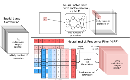
Figure 2: While learning large kernels increases the number of learnable parameters quadratically (left), neural implicit functions use a fixed amount of learnable parameters (top right). When using a simple MLP the input is a 2D vector containing the $x$ and $y$ coordinates of the desired filter position. Our NIFF (bottom right) consists of several 1x1 convolutions which start with an input channel size of two. The two input channels encode the $x$ and $y$ direction respectively. Hence, we do not need to iterate over each coordinate separately. Following we include some hidden layers and activations to learn complex filters. At the last layer, the number of output channels is set to the desired number of element-wise multiplication weights.

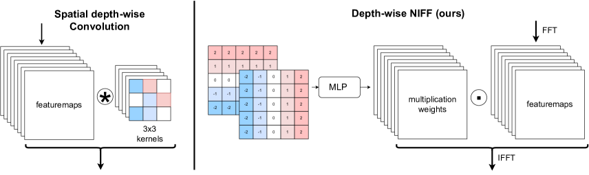
Figure 3: Concept of our NIFF Convolutions, explained with the example of a depthwise convolution. Left, the standard depth-wise convolution in which we have as many kernels as we have featuremaps. Each kernel is convolved with a featuremap. Right, the NIFF convolution consists of two parts. First, an MLP learns based on the coordinates of the frequency spectrum the multiplication weights. Secondly, the multiplication weights are multiplied with the FFT-transformed featuremaps. Lastly, the newly updated featuremaps are transformed back into the spatial domain via inverse FFT (IFFT).

3.1 Neural Implicit Frequency Filters

Commonly real-world signals are captured and stored in a discrete manner. For example, images are typically stored as pixel-wise discrete values. Similarly, the filter weights of CNNs are usually learned and stored as discrete values, i.e. a $3\times 3$ filter has 9 parameters to be learned and stored, a $7\times 7$ filter as in ConvNeXt has 49 parameters and a filter as large as the feature map would require e.g. $224\times 224$ (50176) parameters for ImageNet-sized network input. In this case, it is not affordable to directly learn these filter weights. To address this issue, we propose to parameterize filters by neural implicit functions instead of learning these kernels directly. This is particularly beneficial since we can directly learn such neural implicit filter representations in the frequency domain. Figure 2 visualizes the superiority of neural implicit functions for large kernel sizes.

Thus, we learn a function, $F$, in our case implemented as an MLP, parameterized by $\Phi$ based on the filter frequency array coordinates encoded by $(x,y)$.

$$F_{\Phi}:\mathbb{R}^{2}\mapsto\mathbb{C}^{C},m(x,y):=F_{\Phi}(x,y)\,,$$ (2)

where $C$ is the number of filter channels and the complex-valued $m(x,y)$ in dimension $c$ is the $c$ the filter value in the frequency domain to be multiplied with $\mathcal{F}(g)(x,y)$ for featuremap $g$. Specifically, with the implicit function $F_{\Phi}$, we parameterize the multiplication weights with which the featuremaps are multiplied in the frequency domain based on equation (1) by point-wise multiplication. The number of output channels of the MLP is equivalent to the number of channels $C$ for the convolution and its hidden dimensions determine the expressivity of each learned filter, which we term Neural Implicit Frequency Filter (NIFF).

Efficient Parameterization for Neural Implicit Frequency Filters as Stacked $1\times 1$ Convolutions. While neural implicit functions allow parameterizing large filters with only a few model weights, their direct implementation would be highly inefficient. Therefore, we resume a trick that allows efficient training and inference using standard neural network building blocks. Specifically, we propose to represent the input $(x,y)$ to the MLP by the discrete spatial frequencies for which we need to retrieve filter values and arrange them in 2D arrays that formally resemble feature maps in CNNs but are fixed for all layers. Thus, the MLP gets as input one array encoding the $x$ coordinates and one encoding the $y$ coordinates as shown in Figure 3.

Then, the MLP can be equivalently and efficiently computed using stacked $1\times 1$ convolutions, where the first $1\times 1$ convolution has input depth 2 for the two coordinates and the output layer $1\times 1$ convolution has output dimension $2\times C$ for $C$ complex values filters.

3.2 Common CNN Building Blocks using NIFF

Well-established models like ResNet [18] use full convolutions, while more recent architectures employ depthwise and $1$ convolutions separately [26]. Our neural implicit frequency filters are implemented for all these cases. However, operations including downsampling via stride of two are kept as original spatial convolution. In the following, we describe how commonly used convolution types are implemented using NIFF.

Depth-wise Convolution. For the implementation of the depth-wise convolution, we use the proposed neural implicit function-based NIFF described in 3.1. The module for the depthwise convolution is as follows: First, we transform the feature maps into the frequency domain via FFT and apply FFTshift, i.e., the low-frequency components are shifted to the center. Afterwards, the learned filters are applied via element-wise multiplications with the center-shifted feature maps. Thereafter, the featuremaps are shifted back and transformed back into the spatial domain via inverse FFT (if the next step is to be executed in the spatial domain). The full process is visualized in Figure 3.

Full Convolution. To employ NIFF for a full convolution 2DConv with $C_{p}$ input channels and $C_{q}$ output channels the convolved featuremaps with the kernel weights need to be summed, according to

$$\mathrm{2DConv}(g_{C_{p}},k_{C_{p},C_{q}})=\sum_{c}^{C_{p}}g_{c}\circledast k_{c,C_{q}}=g_{C_{q}}.$$ (3)

Conveniently, a summation in the spatial domain is equivalent to a summation in the frequency domain and can be performed right away.

$$g+k=\mathcal{F}^{-1}(\mathcal{F}(g)+\mathcal{F}(k))$$ (4)

For the full convolution in the frequency domain, we implemented two different approaches. The first one is straightforward by predicting the frequency representation of $k_{C_{p},C_{q}}$ directly using NIFF, i.e. for each output channel, all input channels are element-wise multiplied with the filter weights and summed up in $\mathrm{2DConv}_{\mathit{NIFF}}$:

$$\sum_{c}^{C_{p}}g_{c}\circledast k_{c,C_{q}}=\mathcal{F}^{-1}\left(\sum_{c}^{C_{p}}\mathcal{F}(g_{c})\odot\mathcal{F}(k_{c,C_{q}})\right)$$ (5)

Another approach is to decompose the full convolution into a depth-wise convolution followed by a 1x1 convolution. The transformation into the frequency domain takes place before the depth-wise convolution and the transformation back into the spatial domain is only after the 1x1 convolution. While not being equivalent, the amount of learnable parameters decreases significantly with this approach and the resulting models show similar performance in practice.

$1\times 1$ Convolution. To perform a $1\times 1$ convolution, we transform the input into the frequency domain via FFT. Afterwards, we apply a linear layer with channel input neurons and desired output dimension output neurons on the channel dimension. Finally, we transform back into the spatial domain via inverse FFT. While spatial $1\times 1$ convolutions only combine spatial information in one location, our $1\times 1$ frequency space is able to combine and learn important information globally.

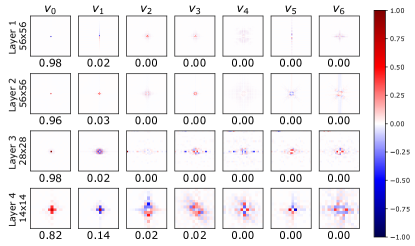
Figure 4: PCA basis and explained variance for each basis vector (below) of all spatial filters for each layer of a ConvNeXt-tiny trained on ImageNet100. On the left, the maximal filter size for the corresponding layer is given. We can see that most filters only use a really small kernel size although they could use a much bigger kernel. Especially for the first layer, the learned filters are really small.

Other operations such as normalization and non-linear activation are applied in the spatial domain so that the resulting models are as close as possible to their spatial domain baselines while enabling infinite-sized convolutions.

4 How large do CNNs spatial kernels really need to be?

After introducing our possibly infinite large frequency filters, we now quantitatively answer the question of how large the spatial kernels really need to be. Hence, we transform the learned filters into the spatial domain and plot the relative density for each spatial kernel $k$, i.e. the ratio of the kernel mass that is contained within centered, smaller sized, squared kernels (i.e. width equals height, denoted as kernel size as in the main paper). The kernel has the same width and height as the feature map (FM) it is convolved to.

$$\mathrm{kernel}\,\mathrm{mass}\,\mathrm{ratio}(\mathrm{width},\mathrm{height})=$$

$$\frac{\displaystyle\sum_{w=1}^{\mathrm{width}}\sum_{h=1}^{\mathrm{height}}k\left(\mathrm{c}-\lfloor\frac{\mathrm{width}}{2}\rfloor+w,\mathrm{c}-\lfloor\frac{\mathrm{height}}{2}\rfloor+h\right)}{\displaystyle\sum_{w=1}^{\mathrm{FMwidth\phantom{.}}}\sum_{h=1}^{\mathrm{FMheight}}(k(w,h))},$$ (6)

where c is the center of the full kernel $k$ in the spatial domain.

In Figure 5 we evaluate the spatial kernel size of networks trained on CIFAR10. For all models, we see a clear trend. They seem to learn in all layers well-localized, small kernels. Yet, a few kernels seem to use the full potential for each kernel size respectively.

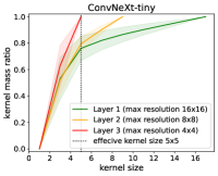
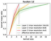
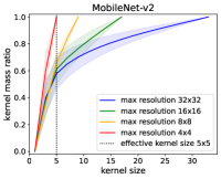
Figure 5: Effective kernel size evaluation on CIFAR-10. We plot the average ratio of the entire kernel mass contained within the limited spatial kernel size, where the x-axis denotes the width and height of the squared kernels. For ResNet-50 and ConvNeXt-tiny each layer encodes one resolution. Thus, the layers could be summarised for ResNet-50 and ConvNeXt-tiny (Layer 1 encoding $16\times 16$, Layer 2 $8\times 8$ and Layer 3 $4\times 4$. However, for MobileNet-v2 the resolution is downsampled within a layer.

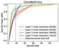
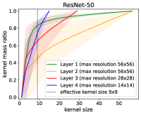
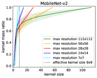
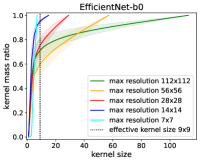
Figure 6: Effective kernel size evaluation on ImageNet-100. We plot the average ratio of the entire kernel mass contained within the limited spatial kernel size, where the x-axis denotes the width and height of the squared kernels. For ResNet-50 and ConvNeXt-tiny each layer encodes one resolution. Thus, the layers could be summarised for ResNet-50 and ConvNeXt-tiny (Layer 1 encoding $56\times 56$, Layer 2 $28\times 28$, Layer 3 $14\times 14$ and Layer 4 $7\times 7$. However, for MobileNet-v2 and EfficientNet-b0 the resolution is downsampled within a layer.

In Figure 6, we report these evaluations for ImageNet-100. We observe that the first, third and fourth layer contain mostly well-localized small kernels for ResNet-50 and ConvNeXt-tiny. Yet, the second layer seems to contain also larger kernels, especially in the case of ResNet-50. For MobileNet-v2 and EfficientNet-b0 the spatial kernels are dominantly well-localized, small kernels. Yet, some kernels seem to be as big as they can, especially for the highest resolution of $112\times 112$.

5 Experiments

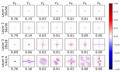
Figure 7: PCA basis and explained variance for each basis vector (below) of all spatial filters for each layer of a ResNet50 trained on ImageNet100. On the left, the maximal filter size for the corresponding layer is given. We can see that most filters only use a really small kernel size although they could use a much bigger kernel. Especially for the first layer, the learned filters are really small.

The evaluation of our proposed NIFF CNNs is done in two parts. First, we analyse the filter weights in the frequency and spatial domain. Therefore we show the filters of the best-performing ResNet18 on CIFAR10 and ResNet50 as well as ConvNeXt-tiny on ImageNet100. The visualizations for further networks coincide with the shown results and are presented in the appendix.

Secondly, we evaluate the performance of NIFF CNNs on high- and low-resolution datasets. The architecture of the NIFFs is dependent on the size of the dataset. Thus, the networks for learning the NIFFs for CIFAR are less complex, hence, smaller (two layers) and for ImageNet more complex, hence, larger (four layers). The exact architecture of our networks for learning the NIFFs is given in the appendix. Moreover, we show an ablation study on the influence of learning the NIFFs.

5.1 Filter Analysis

In this section, we visualize the learned element-wise multiplication weights for the convolution in the frequency domain as well as the spatial kernels which correspond to these frequency filters. Thereby we show that the networks, although they could learn infinitely large kernels, learn well-localized, quite small ($3\times 3$ up to $9\times 9$) kernels. The spatial kernel size is different for low- and high-resolution data.

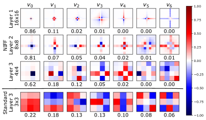
Figure 8: PCA basis and explained variance for each basis vector (below) of all spatial filters learned by NIFF for each layer as well as the learned filters for the first layer of a ResNet18 trained on CIFAR10. On the left, the layer and its filter size are given. We can see that most filters only use a really small kernel size although they could use a much bigger kernel. Especially for the first layer it gets clear that the learned filters are really small.

Figure 7 and Figure 4 visualize the PCAs of the spatial kernel weights for each layer in our NIFF CNNs for a ResNet50 and ConvNeXt-tiny architecture trained on ImageNet100. All layers dominantly learn filters with well-localized, small kernel sizes. Figure 1 shows this fact even clearer. Here the first layer is zoomed in to reveal the learned filter size of about $5\times 5$ although the network could learn filters of size $56\times 56$.

The same effect can be observed for networks trained on CIFAR10. Figure 8 shows the PCAs of the spatial kernel weights for each layer in our NIFF CNNs for a ResNet18 trained on CIFAR10. There the dominant basis vectors for the learned NIFF kernels do not really exceed a size of $3$ in spatial domain.

Further, we analyze the learned element-wise multiplication weights for the real and imaginary parts of a ResNet50 trained on ImageNet100 in the frequency domain. Figure 9 shows the PCA per layer for the learned element-wise multiplication weights. It seems as if the network focuses in the first layer on the middle-frequency spectra and in the later layers more on the high-frequency spectra. Additionally, we see that the imaginary part seems to be less important and thus the learned structures are less complex. This might be owed to the fact that with increased sparsity through the activation function in the network, the network favours cosine structures (structures with a peak in the center) over sine structures.

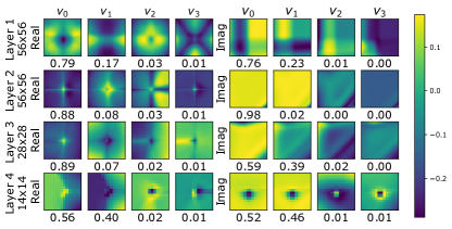
Figure 9: PCA basis and explained variance for each basis vector (below) of all element-wise multiplication weights for the real and imaginary part in the frequency domain for each layer of a ResNet50 trained on ImageNet100. On the left, the maximal filter size for the corresponding layer is given. Right the weights for the real values are given, and on the left are the imaginary values.

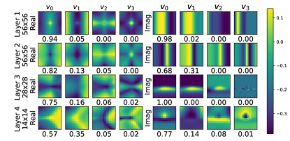
Figure 10: PCA basis and explained variance for each basis vector (below) of all element-wise multiplication weights for the real and imaginary part in the frequency domain for each layer of a ConvNeXt-tiny trained on ImageNet100. On the left, the maximal filter size for the corresponding layer is given. Right the weights for the real values are given, and on the left the imaginary weights.

5.2 Performance Evaluation

We evaluate a variety of networks with our proposed NIFF. Overall we achieve on par performances on classification tasks. For high-resolution data and larger models, our NIFF CNNs perform slightly better than the baseline while the large kernels can apparently not be leveraged for low-resolution data. This could be related to our previous observations that the large size of the filters is not used.

Comparison to previous approaches. We first evaluate our approach against previous attempts to learn convolutions purely in the frequency domain in Table 1. Unfortunately, some approaches did only evaluate the time improvement/ efficiency of the network by using point-wise multiplications instead of the convolution in the spatial domain and missed reporting the achieved accuracy with their networks [29, 52]. Besides those who missed reporting clean accuracies, [34] only reported their accuracy in form of a graph, in which it is hard to get the exact clean accuracy. Hence, we approximate this value. [32] reported different sizes of their CEMNets, thus the accuracy of the networks is reported in the range reported in [32]. Table 1 shows, that our NIFF CNN is the first approach that achieves state-of-the-art performance on CIFAR10. Moreover, we are the first to our knowledge, to report evaluation results on ImageNet100 and ImageNet1k for convolutions purely learned in the frequency domain.

Table 1: Comparison on CIFAR10 of NIFF CNNs to previous approaches which learned convolutions in the frequency domain. While all previous approaches based on CNN architectures could not achieve state-of-the-art performance ours is the first approach. However, [35] can achieve the best performance building upon a Transformer architecture which uses over six (6.2) times more parameters than our lightweight CNN-based NIFF model.

Method	Architecture	Clean Top 1 Acc
Fast FFT [29]	-	no acc. reported
CS-unit [52]	-	no acc. reported
FCNN [34]	FCNN	$\sim$ 30%
CEMNet [32]	CEMNet	59.33%-78.37%
NIFF CNNs (ours)	MobileNet-v2	94.03%
GFN [35]	Swin-Transformer	98.60%

High-resolution data. For high-resolution datasets like ImageNet or ImageNet100, NIFF CNNs are able to achieve on-par results compared to the baseline models. Table 2 as well as A1 present these results. For the heavier models (in terms of learnable parameters) like ResNet [18], DenseNet [19] and also ConvNeXt [26] NIFF performs slightly better than the baseline, while we achieve slightly worse performance on lighter models like MobileNet [39]. For now, we simply used the baseline hyperparameters reported for each of these models by the original authors to stay comparable. Further, we want to emphasize that our NIFF is rather a tool to evaluate the effective kernelsize of CNNs. Yet, we find that achieving the baseline proves our method to be equivalent.

Table 2: Evaluation of top 1 and 5 test accuracy on ImageNet1k for different network architectures. We used the standard training parameter for each network architecture and stayed consistent with these for each architecture respectively. Due to computational constraints, we only report ResNet50 and the smaller MobileNet-v2. We observe a similar trend to ImageNet100, large models benefit from NIFF, while small models do not.

Name	Acc@1	Acc@5	epochs
ConvNeXt-tiny baseline [26]	82.5	96.1	600
ConvNeXt-tiny NIFF (ours)	81.8	95.8	600
ResNet-50 baseline [18]	76.1	92.9	300
ResNet-50 NIFF (ours)	79.7	94.7	300
DenseNet-121 baseline [19]	76.65	92.17	-
DenseNet-121 NIFF (ours)	74.58	92.33	300
MobileNet-v2 baseline [39]	71.8	90.3	150
MobileNet-v2 NIFF (ours)	71.5	90.4	150

Low-resolution data. Although NIFF CNNs can perform on par with high-resolution datasets, their limitations are based on low-resolution dataset. Table 3 shows the results on CIFAR10 with different architectures. Unfortunately, our NIFF CNNs lose around 1 to 3 % points compared to the baseline models. This can be addressed to our previous observation: The networks trained on CIFAR10 do only use a small amount of the potential kernel size NIFF provides being as big as the kernels of the baseline model ($3\times 3$).

Table 3: Performance evaluation of different networks trained on CIFAR10. To be comparable between all models and architecture changes we used the same training schedule for all of them. One can see that NIFF CNNs perform slightly better with a ConvNeXt [26] backbone. However, for other architectures, it performs slightly worse.

Method	Architecture	Clean Top 1 Acc
Baseline [26]	ConvNeXt-tiny	90.37
NIFF relu	ConvNeXt-tiny	91.48
NIFF silu	ConvNeXt-tiny	91.45
Baseline [18]	ResNet-18	92.74
NIFF relu	ResNet-18	90.63
NIFF silu	ResNet-18	90.12
Baseline [19]	DenseNet-121	93.93
NIFF relu	DenseNet-121	92.49
NIFF silu	DenseNet-121	92.20
Baseline [39]	MobileNet-v2	94.51
NIFF relu	MobileNet-v2	94.03
NIFF silu	MobileNet-v2	93.84

6 Discussion

Filter Analysis. Our NIFF is, for now, mainly a tool to evaluate the real importance of kernel sizes in current image classification tasks. Thus, we want to discuss the overall takeaway that we could show. As with the development of vision transformer [12, 21, 48, 50], new CNN architectures [26] and combination of both world [11, 24, 25] which all include some kind of larger receptive fields compared to previous networks [18, 19] we wanted to ask the question: How large do CNN kernels really need to be?

With the help of our proposed novel NIFF, we can analyze the actually learned kernel size in the spatial domain of state-of-the-art networks. We could observe that the full potential for much larger receptive fields is not used in most models. Especially for low-resolution datasets like CIFAR10, the network refuses to learn much bigger kernels than $3\times 3$. Thus, state-of-the-art networks on CIFAR are already optimized in terms of kernel sizes used. However, on high-resolution datasets like ImageNet, the network indeed uses larger kernel sizes than $3\times 3$ but still not much larger than $9\times 9$. Hence, networks with small kernel sizes like ResNet [18] could benefit from larger kernel sizes, while networks like ConvNeXt [26] are also already close to optimal for ImageNet in terms of used kernel size.

One point why large kernel sizes are still less used is the computational overhead, one gets as well as possible leakage artifacts as described by [47]. Regarding the computational efficiency, we propose our NIFF to learn the filters and thus use much fewer parameters. We assume that applying a hamming window as in [47] might be useful in our case too. However, we leave this for future research, as we focus here on the analysis.

Performance Evaluation. We can observe that NIFF achieves results on par with spatial baseline models on high-resolution classification tasks and can even improve over the baseline leveraging expressive architectures such as ResNet-50 without an increase in learnable parameters. Further, we emphasize that the used hyperparameters are simply the ones used for standard training in the spatial domain. We strongly believe that optimizing the hyperparameters specifically for NIFF might yield a further performance boost. Moreover, we see a strong potential of NIFF for high-resolution datasets like ImageNet or even larger datasets, as it is designed to enhance large receptive fields.

Limitations. For now, including our NIFF in state-of-the-art CNNs requires the switching between spatial and frequency domain for normalization and non-linearity, leading to a computational overhead of using FFT and inverse FFT. Hence, we suggest for future research to implement the full network in the frequency domain by shifting not only the convolution in the frequency domain but also, batch normalization, activation function and the fully connected part to be executed on the frequency channels rather than the spatial channels.

7 Conclusion

We develop NIFF CNNs, a tool with which we can learn convolution filters that translate to infinitely large kernels in the spatial domain. NIFF can replace common spatial convolutions with an element-wise multiplication in the frequency domain. We analyse the resulting kernels in the frequency domain as well as in the spatial domain and observe that the learned kernels in the spatial domain are still well-localized and quite small ($9\times 9$) given the fact that they could be much larger ($224\times 224$). This effect is even stronger for low-resolution datasets leading to worse performance for these cases. On large-scale datasets, NIFF can perform on par with or better than spatial convolutions.

As large as it gets: Learning infinitely large Filters via Neural Implicit Functions
Supplementary Material

In the following, we provide additional information and details that accompany the main paper:

• A - additional filter visualizations

• B - more results on ImageNet-100

• C - details on NIFF runtimes

• D - additional details on the NIFF architecture

• E - details on training parameters

Appendix A Filter Visualization

In this section, we show the PCA evaluation of the learned NIFFs (Figure A1 and A2) for different network architectures trained on ImageNet-100 as well as their spatial representations (Figure A3 and A4).

We observe similar behaviour as shown in Figure 9 and 10 in the main paper for the PCA of the learned NIFFs. For the imaginary part, the networks learn less complex structures, while for the real part, the stacked $1\times 1$ convolutions learn filters either concentrated on the high or low-frequency information for each layer.

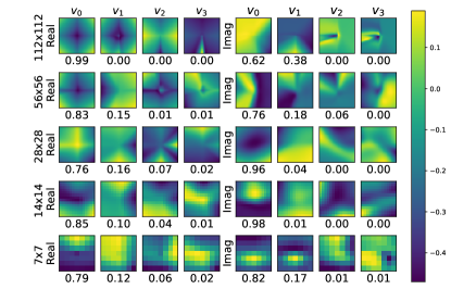
Figure A1: PCA basis and explained variance for each basis vector (below) of all element-wise multiplication weights for the real and imaginary part in the frequency domain for each filter resolution of a MobileNet-v2 trained on ImageNet-100. On the right, the maximal filter size for the corresponding layer is given. Right the weights for the real values are given, and on the left the ones for the imaginary part.

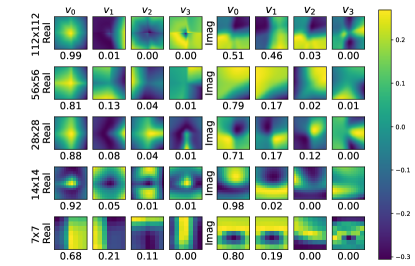
Figure A2: PCA basis and explained variance for each basis vector (below) of all element-wise multiplication weights for the real and imaginary part in the frequency domain for each filter resolution of an EfficientNet-b0 trained on ImageNet-100. On the right, the maximal filter size for the corresponding layer is given. Right the weights for the real values are given, and on the left the ones for the imaginary part.

The PCAs of the spatial kernels (Figure A3 and A4) show similar behaviour as already observed. The learned filters in the spatial domain are well-localized and relatively small compared to the size they could actually learn.

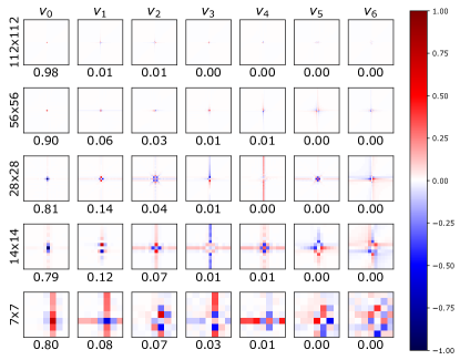
Figure A3: PCA basis and explained variance for each basis vector (below) of all spatial filters for each resolution for the convolutions of a MobileNet-V2 trained on ImageNet-100. On the right, the maximal filter size for the corresponding layer is given. We can see that most filters only use a really small kernel size although they could use much bigger kernels. Especially for the first layer it gets clear that the learned filters are really small.

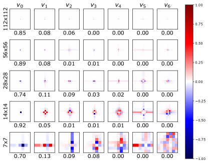
Figure A4: PCA basis and explained variance for each basis vector (below) of all spatial filters for each resolution for the convolutions of an EfficientNet-b0 trained on ImageNet-100. On the right, the maximal filter size for the corresponding layer is given. We can see that most filters only use a really small kernel size although they could use much bigger kernels. Especially for the first layer it gets clear that the learned filters are really small.

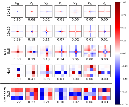
Figure A5: PCA basis and explained variance for each basis vector (below) of all spatial filters for each resolution for the convolutions of a MobileNet-V2 trained on CIFAR-10. On the right, the maximal filter size for the corresponding layer is given. We can see that most filters only use a really small kernel size although they could use much bigger kernels. Especially for the first layer it gets clear that the learned filters are really small.

The learned spatial filters on CIFAR10 are shown in Figure A5. Similarly, to the results shown in Figure 8. The network learns well-localized, small filters n the spatial domain. Yet, for the kernel size of $8\times 8$ the network uses more than the standard kernel size of $3\times 3$.

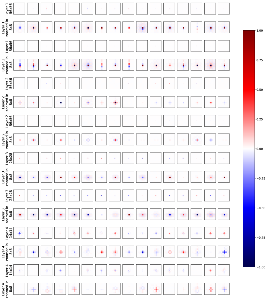
Figure A6: Actual kernels in the spatial domain of a ConvNeXt-tiny including NIFF with a SiLU activation trained on ImageNet-100. We plot for each kernel the zoomed-in version below for better visibility. Overall, most kernels exhibit well-localized, small spatial kernels.

Further, we show a grid of the actually learned filter in the spatial domain in Figure A6.

Appendix B ImageNet-100 for more Models

We report the numbers our NIFF CNNs could achieve on ImageNet-100 in Table A1. The trend is similar to ImageNet-1k, the larger models benefit from NIFF while the lightweight models do not so much.

Additionally, we report two different versions of our NIFF. One including ReLU activation and one including SiLU activation.

Table A1: Performance evaluation of top 1 and 5 test accuracy on ImageNet100 for different network architectures. We used the standard training parameter for each network architecture and stayed consistent with these for each architecture respectively. For the bigger networks like ResNet and DenseNet, which include full convolutions split into depth-wise and 1x1 convolution as described in Section 3.2 to reduce the number of parameters, for faster training. For larger models, our NIFF CNNs perform slightly better, even with the reduced number of parameters.

Name	# Parameters	Acc@1	Acc@5
ConvNeXt-tiny [26]	27.897.028	91.70	98.32
NIFF relu	28.231.684	91.12	98.34
NIFF silu	28.231.684	92.00	98.42
ResNet-50 [18]	23.712.932	89.88	98.22
NIFF relu	16.760.900	89.86	98.16
NIFF silu	16.760.900	89.98	98.44
DenseNet-121 [19]	7.056.356	90.06	98.20
NIFF relu	5.237.012	90.14	98.16
NIFF silu	5.237.012	90.24	98.18
EfficientNet-b0 [46]	4.135.648	87.10	97.52
NIFF relu	4.047.236	86.80	97.52
NIFF silu	4.047.236	86.66	97.36
MobileNet-v2 [39]	2.351.972	84.06	96.52
NIFF relu	2.359.660	84.08	96.66
NIFF silu	2.359.660	85.46	96.70

Appendix C Runtime

Since our NIFF implementation is conceived for analysis purposes, our models are not optimized with respect to runtime. In particular, we compute repeated FFTs in pytorch to allow the computation of non-linear activations in the spatial domain, so that the models remain equivalent to large kernel models computed in the spatial domain. Nonetheless, we evaluate here the runtime per epoch during training. For the comparison, we used the ResNet-18 trained on CIFAR10. We observe that networks including NIFF with either ReLU or SiLU activation and the $1\times 1$ convolution in the frequency domain do take around twice as long as (e.g. $17.6$ secs per epoch on one NVIDIA TITAN V) the baseline network (e.g. $8.8$ secs per epoch on one NVIDIA TITAN V), which is reasonably fast, considering the repeated Fourier transforms. Further, we compared the runtime for a simple 2D convolution and one which includes the transformation into the frequency domain via FFT and back into the spatial domain via inverse FFT beforehand. We observed a time increase of around $40\%$ to $70\%$ depending on the featuremap size.

For transparency, we evaluate the runtime per epoch for each model on CIFAR10 and ImageNet and compare it to the standard spatial 3x3 convolution, which has a much smaller receptive field than our NIFF. Additionally, we evaluate spatial 9x9 convolutions, which is the average spatial filtersize of the used NIFF. However, we want to emphasize that our NIFF models still learned infinite large kernels while all kernels in the spatial domain are limited to the set kernel size.

Table A2: Average training time per epoch in seconds on one NVIDIA Titan of NIFF compared to standard 3x3 (or 7x7 for ConvNeXt) spatial convolutions and larger 9x9 spatial convolutions on CIFAR10.

Name	3x3/7x7	9x9	NIFF (ours)
ConvNeXt-tiny [26]	149.37	152.23	85.75
ResNet-18 [18]	8.78	32.74	17.58
DenseNet-121 [19]	26.16	35.52	83.22
MobileNet-v2 [39]	22.35	42.06	83.94

Table A3: Average training time per epoch in seconds on four NVIDIA A100 of NIFF compared to standard 3x3 (or 7x7 for ConvNeXt) spatial convolutions and larger 9x9 spatial convolutions on ImageNet100.

Name	3x3/7x7	9x9	NIFF(ours)
ConvNeXt-tiny [26]	95.43	103.69	151.77
ResNet-50 [18]	85.51	133.28	204.82
DenseNet-121 [19]	128.85	148.30	400.61
EfficientNet-b0 [46]	45.01	141.14	111.40
MobileNet-v2 [39]	34.13	93.55	101.39

Appendix D NIFFs architecture

Following we will describe the architecture used for our NIFFs for each backbone network architecture. Note that the size of the NIFF is adjusted to the size of the baseline network as well as the complexity of the classification task.

Low-resolution task

All networks trained on CIFAR10 incorporate the same NIFF architecture. The NIFF consists of two stacked $1\times 1$ convolutions with an activation function in between. The $1\times 1$ convolution receives as input two channels, which encode the $x$ and $y$ coordinate as described in Figure 2. The $1\times 1$ convolution expands these two channels to 32 channels. From these 32 channels, the next $1\times 1$ convolution maps the 32 channels to the desired number of point-wise multiplication weights. As activation, we used ReLU or SiLU as well as GeLU. However, GeLU did not perform as well as ReLU and SiLU. Hence, we stick to ReLU and SiLU for further experiments. The ablation of the used activation can be found in Table A4.

Table A4: Evaluation of top 1 accuracy on CIFAR-10 for different activation function within out NIFF.

Name	Acc@1
Baseline	92.74
ReLU	90.63
SiLU	90.12
GeLU	89.18

High-resolution task

For the networks trained on ImageNet-100 and ImageNet-1k the size of the neural implicit function to predict the NIFF is kept the same for each architecture respectively. Yet, the size of the neural implicit function is adjusted to the network architecture to achieve approximately the same number of trainable parameters. Hence, lightweight models like MobileNet-v2 [39] or EfficientNet-b0 [46] incorporate a smaller light-weight neural implicit function to predict the NIFF, while larger models like ResNet-50 [18], DenseNet-121 [19] or ConvNeXt-tiny [26] incorporate a larger neural implicit function. For simplicity, we define two NIFF architectures. One for the large models and one for the lightweight models.

For the lightweight models, the neural implicit function consists of three stacked $1\times 1$ convolutions with one activation after the first one and one after the second one. The activation is kept the same, either ReLU or SiLU. The dimensions for the three $1\times 1$ convolutions are as follows. We start with two channels and expand to eight channels. From these eight channels, the second $1\times 1$ convolution suppresses the channels down to four. Afterwards, the last $1\times 1$ convolution maps these four channels to the desired number of point-wise multiplication weights.

For the larger models, we used four layers within the neural implicit function for NIFF. The structure is similar to all NIFFs between each $1\times 1$ convolution an activation function is applied, either ReLU or SiLU. The dimensions for the four layers are as follows. First from two to 16 channels, secondly from 16 to 128 channels and afterwards suppressed down from 128 to 32 channels. The last $1\times 1$ convolution maps these 32 channels to the desired number of point-wise multiplication weights.

We show that the smaller NIFF size for the lightweight models does not influence the resulting performance. Thus, we train the lightweight models with larger NIFFs (similar size as the larger models). The results are presented in Table A5. We can see that the networks do not benefit from the larger NIFF size. Hence, we assume that keeping the smaller NIFFs for lightweight models can achieve a good trade-off between the number of learnable parameters and performance.

Table A5: Evaluation of top 1 and top 5 accuracies on ImageNet-100 for different NIFF sizes in lightweight models.

Name	Acc@1	Acc@5
MobileNet-v baseline	84.94	96.28
small NIFF silu	83.72	96.40
small NIFF relu	84.08	96.66
big NIFF silu	83.82	96.32
big NIFF relu	83.14	96.56
EfficientNet-b0 baseline	87.10	97.52
small NIFF silu	86.66	97.36
small NIFF relu	86.80	97.52
big NIFF silu	86.56	97.60
big NIFF relu	86.94	97.20

Appendix E Training Details

CIFAR10.

For CIFAR10 we used the same training parameter for all networks. We trained each network for 150 epochs with a batch size of 256 and a cosine learning rate schedule with a learning rate of 0.02. we set the momentum to 0.9 and weight decay to 0.002. The loss is calculated via LabelSmoothingLoss with label smoothing of 0.1 and as an optimizer, we use Stochastic Gradient Descent (SGD).

For data preprocessing we simply used zero padding by four and cropping back to $32\times 32$ and horizontal flip, as well as normalizing with mean and standard deviation.

ImageNet.

The training parameters and data preprocessing are kept the same for ImageNet-100 as well as ImageNet-1k. For the training of each network architecture, we used the data preprocessing pipeline provided by [26]. Yet, the training parameters for each individual network are taken from the original papers provided by the authors ResNet-50 [18], DenseNet-121 [19] ConvNeXt-tiny [26], MobileNet-v2 [39] and EfficientNet-b0 [46].

References

- [1] Matan Atzmon and Yaron Lipman. Sal: Sign agnostic learning of shapes from raw data. In Proceedings of the IEEE/CVF Conference on Computer Vision and Pattern Recognition, pages 2565–2574, 2020.
- [2] Sayed Omid Ayat, Mohamed Khalil-Hani, Ab Al-Hadi Ab Rahman, and Hamdan Abdellatef. Spectral-based convolutional neural network without multiple spatial-frequency domain switchings. Neurocomputing, 364:152–167, 2019.
- [3] Rohan Chabra, Jan E Lenssen, Eddy Ilg, Tanner Schmidt, Julian Straub, Steven Lovegrove, and Richard Newcombe. Deep local shapes: Learning local sdf priors for detailed 3d reconstruction. In Computer Vision–ECCV 2020: 16th European Conference, Glasgow, UK, August 23–28, 2020, Proceedings, Part XXIX 16, pages 608–625. Springer, 2020.
- [4] Yinbo Chen, Sifei Liu, and Xiaolong Wang. Learning continuous image representation with local implicit image function. In Proceedings of the IEEE/CVF conference on computer vision and pattern recognition, pages 8628–8638, 2021.
- [5] Zhiqin Chen and Hao Zhang. Learning implicit fields for generative shape modeling. In Proceedings of the IEEE/CVF Conference on Computer Vision and Pattern Recognition, pages 5939–5948, 2019.
- [6] Lu Chi, Borui Jiang, and Yadong Mu. Fast fourier convolution. In H. Larochelle, M. Ranzato, R. Hadsell, M.F. Balcan, and H. Lin, editors, Advances in Neural Information Processing Systems, volume 33, pages 4479–4488. Curran Associates, Inc., 2020.
- [7] Julian Chibane, Thiemo Alldieck, and Gerard Pons-Moll. Implicit functions in feature space for 3d shape reconstruction and completion. In Proceedings of the IEEE/CVF Conference on Computer Vision and Pattern Recognition (CVPR), June 2020.
- [8] Julian Chibane, Mohamad Aymen mir, and Gerard Pons-Moll. Neural unsigned distance fields for implicit function learning. In H. Larochelle, M. Ranzato, R. Hadsell, M.F. Balcan, and H. Lin, editors, Advances in Neural Information Processing Systems, volume 33, pages 21638–21652. Curran Associates, Inc., 2020.
- [9] Julian Chibane and Gerard Pons-Moll. Implicit feature networks for texture completion from partial 3d data. In Computer Vision–ECCV 2020 Workshops: Glasgow, UK, August 23–28, 2020, Proceedings, Part II 16, pages 717–725. Springer, 2020.
- [10] Xiaohan Ding, Xiangyu Zhang, Jungong Han, and Guiguang Ding. Scaling up your kernels to 31x31: Revisiting large kernel design in cnns. In Proceedings of the IEEE/CVF Conference on Computer Vision and Pattern Recognition (CVPR), pages 11963–11975, June 2022.
- [11] Xiaoyi Dong, Jianmin Bao, Dongdong Chen, Weiming Zhang, Nenghai Yu, Lu Yuan, Dong Chen, and Baining Guo. Cswin transformer: A general vision transformer backbone with cross-shaped windows. In Proceedings of the IEEE/CVF Conference on Computer Vision and Pattern Recognition, pages 12124–12134, 2022.
- [12] Alexey Dosovitskiy, Lucas Beyer, Alexander Kolesnikov, Dirk Weissenborn, Xiaohua Zhai, Thomas Unterthiner, Mostafa Dehghani, Matthias Minderer, Georg Heigold, Sylvain Gelly, et al. An image is worth 16x16 words: Transformers for image recognition at scale. arXiv preprint arXiv:2010.11929, 2020.
- [13] D. Forsyth and J. Ponce. Computer Vision: A Modern Approach. An Alan R. Apt book. Prentice Hall, 2003.
- [14] Amos Gropp, Lior Yariv, Niv Haim, Matan Atzmon, and Yaron Lipman. Implicit geometric regularization for learning shapes. arXiv preprint arXiv:2002.10099, 2020.
- [15] Bochen Guan, Jinnian Zhang, William A Sethares, Richard Kijowski, and Fang Liu. Specnet: spectral domain convolutional neural network. arXiv preprint arXiv:1905.10915, 2019.
- [16] Meng-Hao Guo, Cheng-Ze Lu, Qibin Hou, Zhengning Liu, Ming-Ming Cheng, and Shi-Min Hu. Segnext: Rethinking convolutional attention design for semantic segmentation. arXiv preprint arXiv:2209.08575, 2022.
- [17] David Ha, Andrew Dai, and Quoc V Le. Hypernetworks. arXiv preprint arXiv:1609.09106, 2016.
- [18] Kaiming He, Xiangyu Zhang, Shaoqing Ren, and Jian Sun. Deep residual learning for image recognition. In Proceedings of the IEEE conference on computer vision and pattern recognition, pages 770–778, 2016.
- [19] Gao Huang, Zhuang Liu, Laurens Van Der Maaten, and Kilian Q Weinberger. Densely connected convolutional networks. In Proceedings of the IEEE conference on computer vision and pattern recognition, pages 4700–4708, 2017.
- [20] Chiyu Jiang, Avneesh Sud, Ameesh Makadia, Jingwei Huang, Matthias Nießner, Thomas Funkhouser, et al. Local implicit grid representations for 3d scenes. In Proceedings of the IEEE/CVF Conference on Computer Vision and Pattern Recognition, pages 6001–6010, 2020.
- [21] Salman Khan, Muzammal Naseer, Munawar Hayat, Syed Waqas Zamir, Fahad Shahbaz Khan, and Mubarak Shah. Transformers in vision: A survey. ACM computing surveys (CSUR), 54(10s):1–41, 2022.
- [22] Alex Krizhevsky, Ilya Sutskever, and Geoffrey E Hinton. Imagenet classification with deep convolutional neural networks. In F. Pereira, C.J. Burges, L. Bottou, and K.Q. Weinberger, editors, Advances in Neural Information Processing Systems, volume 25. Curran Associates, Inc., 2012.
- [23] Shiwei Liu, Tianlong Chen, Xiaohan Chen, Xuxi Chen, Qiao Xiao, Boqian Wu, Mykola Pechenizkiy, Decebal Mocanu, and Zhangyang Wang. More convnets in the 2020s: Scaling up kernels beyond 51x51 using sparsity. arXiv preprint arXiv:2207.03620, 2022.
- [24] Ze Liu, Han Hu, Yutong Lin, Zhuliang Yao, Zhenda Xie, Yixuan Wei, Jia Ning, Yue Cao, Zheng Zhang, Li Dong, et al. Swin transformer v2: Scaling up capacity and resolution. In Proceedings of the IEEE/CVF conference on computer vision and pattern recognition, pages 12009–12019, 2022.
- [25] Ze Liu, Yutong Lin, Yue Cao, Han Hu, Yixuan Wei, Zheng Zhang, Stephen Lin, and Baining Guo. Swin transformer: Hierarchical vision transformer using shifted windows. In Proceedings of the IEEE/CVF international conference on computer vision, pages 10012–10022, 2021.
- [26] Zhuang Liu, Hanzi Mao, Chao-Yuan Wu, Christoph Feichtenhofer, Trevor Darrell, and Saining Xie. A convnet for the 2020s. Proceedings of the IEEE/CVF Conference on Computer Vision and Pattern Recognition (CVPR), 2022.
- [27] Tianyu Ma, Adrian V Dalca, and Mert R Sabuncu. Hyper-convolution networks for biomedical image segmentation. In Proceedings of the IEEE/CVF Winter Conference on Applications of Computer Vision, pages 1933–1942, 2022.
- [28] Tianyu Ma, Alan Q. Wang, Adrian V. Dalca, and Mert R. Sabuncu. Hyper-convolutions via implicit kernels for medical image analysis. Medical Image Analysis, 86:102796, 2023.
- [29] Michael Mathieu, Mikael Henaff, and Yann LeCun. Fast training of convolutional networks through ffts. arXiv preprint arXiv:1312.5851, 2013.
- [30] Ben Mildenhall, Pratul P Srinivasan, Matthew Tancik, Jonathan T Barron, Ravi Ramamoorthi, and Ren Ng. Nerf: Representing scenes as neural radiance fields for view synthesis. Communications of the ACM, 65(1):99–106, 2021.
- [31] Michael Niemeyer, Lars Mescheder, Michael Oechsle, and Andreas Geiger. Differentiable volumetric rendering: Learning implicit 3d representations without 3d supervision. In Proceedings of the IEEE/CVF Conference on Computer Vision and Pattern Recognition, pages 3504–3515, 2020.
- [32] Hengyue Pan, Yixin Chen, Xin Niu, Wenbo Zhou, and Dongsheng Li. Learning convolutional neural networks in the frequency domain, 2022.
- [33] Chao Peng, Xiangyu Zhang, Gang Yu, Guiming Luo, and Jian Sun. Large kernel matters – improve semantic segmentation by global convolutional network. In Proceedings of the IEEE Conference on Computer Vision and Pattern Recognition (CVPR), July 2017.
- [34] Harry Pratt, Bryan Williams, Frans Coenen, and Yalin Zheng. Fcnn: Fourier convolutional neural networks. In Michelangelo Ceci, Jaakko Hollmén, Ljupčo Todorovski, Celine Vens, and Sašo Džeroski, editors, Machine Learning and Knowledge Discovery in Databases, pages 786–798, Cham, 2017. Springer International Publishing.
- [35] Yongming Rao, Wenliang Zhao, Zheng Zhu, Jiwen Lu, and Jie Zhou. Global filter networks for image classification. In A. Beygelzimer, Y. Dauphin, P. Liang, and J. Wortman Vaughan, editors, Advances in Neural Information Processing Systems, 2021.
- [36] David W. Romero, Robert-Jan Bruintjes, Jakub Mikolaj Tomczak, Erik J Bekkers, Mark Hoogendoorn, and Jan van Gemert. Flexconv: Continuous kernel convolutions with differentiable kernel sizes. In International Conference on Learning Representations, 2022.
- [37] David W. Romero, Anna Kuzina, Erik J Bekkers, Jakub Mikolaj Tomczak, and Mark Hoogendoorn. CKConv: Continuous kernel convolution for sequential data. In International Conference on Learning Representations, 2022.
- [38] Shunsuke Saito, Zeng Huang, Ryota Natsume, Shigeo Morishima, Angjoo Kanazawa, and Hao Li. Pifu: Pixel-aligned implicit function for high-resolution clothed human digitization. In Proceedings of the IEEE/CVF international conference on computer vision, pages 2304–2314, 2019.
- [39] Mark Sandler, Andrew Howard, Menglong Zhu, Andrey Zhmoginov, and Liang-Chieh Chen. Mobilenetv2: Inverted residuals and linear bottlenecks. In Proceedings of the IEEE conference on computer vision and pattern recognition, pages 4510–4520, 2018.
- [40] Karen Simonyan and Andrew Zisserman. Very deep convolutional networks for large-scale image recognition. arXiv preprint arXiv:1409.1556, 2014.
- [41] Vincent Sitzmann, Julien Martel, Alexander Bergman, David Lindell, and Gordon Wetzstein. Implicit neural representations with periodic activation functions. In H. Larochelle, M. Ranzato, R. Hadsell, M.F. Balcan, and H. Lin, editors, Advances in Neural Information Processing Systems, volume 33, pages 7462–7473. Curran Associates, Inc., 2020.
- [42] Vincent Sitzmann, Michael Zollhöfer, and Gordon Wetzstein. Scene representation networks: Continuous 3d-structure-aware neural scene representations. Advances in Neural Information Processing Systems, 32, 2019.
- [43] Christian Szegedy, Sergey Ioffe, Vincent Vanhoucke, and Alexander Alemi. Inception-v4, inception-resnet and the impact of residual connections on learning. In Proceedings of the AAAI conference on artificial intelligence, volume 31, 2017.
- [44] Christian Szegedy, Wei Liu, Yangqing Jia, Pierre Sermanet, Scott Reed, Dragomir Anguelov, Dumitru Erhan, Vincent Vanhoucke, and Andrew Rabinovich. Going deeper with convolutions. In Proceedings of the IEEE conference on computer vision and pattern recognition, pages 1–9, 2015.
- [45] Christian Szegedy, Vincent Vanhoucke, Sergey Ioffe, Jon Shlens, and Zbigniew Wojna. Rethinking the inception architecture for computer vision. In Proceedings of the IEEE conference on computer vision and pattern recognition, pages 2818–2826, 2016.
- [46] Mingxing Tan and Quoc Le. Efficientnet: Rethinking model scaling for convolutional neural networks. In International conference on machine learning, pages 6105–6114. PMLR, 2019.
- [47] Nergis Tomen and Jan C van Gemert. Spectral leakage and rethinking the kernel size in cnns. In Proceedings of the IEEE/CVF International Conference on Computer Vision, pages 5138–5147, 2021.
- [48] Hugo Touvron, Matthieu Cord, Matthijs Douze, Francisco Massa, Alexandre Sablayrolles, and Hervé Jégou. Training data-efficient image transformers & distillation through attention. In International conference on machine learning, pages 10347–10357. PMLR, 2021.
- [49] Nicolas Vasilache, Jeff Johnson, Michael Mathieu, Soumith Chintala, Serkan Piantino, and Yann LeCun. Fast convolutional nets with fbfft: A gpu performance evaluation. arXiv preprint arXiv:1412.7580, 2014.
- [50] Ashish Vaswani, Noam Shazeer, Niki Parmar, Jakob Uszkoreit, Llion Jones, Aidan N Gomez, Łukasz Kaiser, and Illia Polosukhin. Attention is all you need. Advances in neural information processing systems, 30, 2017.
- [51] Shenlong Wang, Simon Suo, Wei-Chiu Ma, Andrei Pokrovsky, and Raquel Urtasun. Deep parametric continuous convolutional neural networks. In Proceedings of the IEEE Conference on Computer Vision and Pattern Recognition (CVPR), June 2018.
- [52] Zelong Wang, Qiang Lan, Dafei Huang, and Mei Wen. Combining fft and spectral-pooling for efficient convolution neural network model. In 2016 2nd International Conference on Artificial Intelligence and Industrial Engineering (AIIE 2016), pages 203–206. Atlantis Press, 2016.
- [53] Thomio Watanabe and Denis F Wolf. Image classification in frequency domain with 2srelu: a second harmonics superposition activation function. Applied Soft Computing, 112:107851, 2021.
- [54] Alex Yu, Vickie Ye, Matthew Tancik, and Angjoo Kanazawa. pixelnerf: Neural radiance fields from one or few images. In Proceedings of the IEEE/CVF Conference on Computer Vision and Pattern Recognition, pages 4578–4587, 2021.