TinyTrain: Deep Neural Network Training at the Extreme Edge

Young D. Kwon¹ Rui Li² Stylianos I. Venieris²
Jagmohan Chauhan³ Nicholas D. Lane^1,2 Cecilia Mascolo¹
¹University of Cambridge, UK
²Samsung AI Center, Cambridge
³University of Southampton, UK
{ydk21,nd132,cm542}@cam.ac.uk {s.venieris,rui.li}@samsung.com J.Chauhan@soton.ac.uk

Abstract

On-device training is essential for user personalisation and privacy. With the pervasiveness of IoT devices and microcontroller units (MCU), this task becomes more challenging due to the constrained memory and compute resources, and the limited availability of labelled user data. Nonetheless, prior works neglect the data scarcity issue, require excessively long training time (e.g. a few hours), or induce substantial accuracy loss ( $\geq$ 10%). We propose TinyTrain, an on-device training approach that drastically reduces training time by selectively updating parts of the model and explicitly coping with data scarcity. TinyTrain introduces a task-adaptive sparse-update method that dynamically selects the layer/channel based on a multi-objective criterion that jointly captures user data, the memory, and the compute capabilities of the target device, leading to high accuracy on unseen tasks with reduced computation and memory footprint. TinyTrain outperforms vanilla fine-tuning of the entire network by 3.6-5.0% in accuracy, while reducing the backward-pass memory and computation cost by up to 2,286 $\times$ and 7.68 $\times$ , respectively. Targeting broadly used real-world edge devices, TinyTrain achieves 9.5 $\times$ faster and 3.5 $\times$ more energy-efficient training over status-quo approaches, and 2.8 $\times$ smaller memory footprint than SOTA approaches, while remaining within the 1 MB memory envelope of MCU-grade platforms.

1 Introduction

On-device training of deep neural networks (DNNs) on edge devices has the potential to enable diverse real-world applications to dynamically adapt to new tasks [40] and different (i.e. cross-domain/out-of-domain) data distributions from users (e.g. personalisation) [38], without jeopardising privacy over sensitive data (e.g. healthcare) [12].

Despite its benefits, several challenges hinder the broader adoption of on-device training. Firstly, labelled user data are neither abundant nor readily available in real-world IoT applications. Secondly, edge devices are often characterised by severely limited memory. With the forward and backward passes of DNN training being significantly memory-hungry, there is a mismatch between memory requirements and memory availability at the extreme edge. Even architectures tailored to microcontroller units (MCUs), such as MCUNet [30], require almost 1 GB of training-time memory (see Table 2), which far exceeds the RAM size of widely used embedded devices, such as Raspberry Pi Zero 2 (512 MB), and commodity MCUs (1 MB). Lastly, on-device training is limited by the constrained processing capabilities of edge devices, with training requiring at least 3 $\times$ more computation (i.e. multiply-accumulate (MAC) count) than inference [61]. This places an excessive burden on tiny edge devices that host less powerful CPUs, compared to the server-grade CPUs or GPUs [31].

Recently, on-device training works have been proposed. These, however, have limitations. First, fine-tuning only the last layer [28, 45] leads to considerable accuracy loss ( $>$ 10%) that far exceeds the typical drop tolerance. Moreover, memory-saving techniques by means of recomputation [6, 41, 58, 12] that trade-off more computation for lower memory usage, incur significant computation overhead, further increasing the already excessive on-device training time. Lastly, sparse-update methods [43, 31, 4] selectively update only a subset of layers and channels during on-device training, effectively reducing both memory and computation loads. Nonetheless, as shown in §3.2, the performance of these approaches drop dramatically (up to 7.7% for SparseUpdate [31]) when applied at the extreme edge where data availability is low. Also, these methods require running a few thousands of computationally heavy search [31] or pruning [43] processes on powerful GPUs to identify important layers/channels for each target dataset, unable to adapt to the properties of the user data on the fly.

Refer to caption — Figure 1: Cross-domain accuracy (y-axis) and compute cost in MAC count (x-axis) of TinyTrain and existing methods, targeting MobileNetV2 on Meta-Dataset. The radius of the circles and the corresponding text denote the increase in the memory footprint of each baseline over TinyTrain. The dotted line represents the accuracy without on-device training.

To address the aforementioned challenges and limitations, we present TinyTrain, the first approach that fully enables compute-, memory-, and data-efficient on-device training on constrained edge devices. TinyTrain departs from the static configuration of the sparse-update policy, i.e. the subset of layers and channels to be fine-tuned being fixed, and proposes task-adaptive sparse update. Our task-adaptive sparse update requires running only once for each target dataset and can be efficiently executed on resource-constrained edge devices. This enables us to adapt the layer/channel selection in a task-adaptive manner, leading to better on-device adaptation and higher accuracy. Specifically, we introduce a novel multi-objective criterion to guide the layer/channel selection process that captures both the importance of channels and their computational and memory cost. Then, at run time, we propose a dynamic layer/channel selection scheme that dynamically adapts the sparse update policy using our multi-objective criterion. As TinyTrain takes into account both the properties of the user data, and the memory and processing capacity of the target device, TinyTrain enables on-device training with a significant reduction in memory and computation without accuracy loss over the state-of-the-art (SOTA) [31]. Finally, to further address the drawbacks of data scarcity, TinyTrain enhances the conventional on-device training pipeline by means of a few-shot learning (FSL) pre-training scheme; this step meta-learns a reasonable global representation that allows on-device training to be sample-efficient and reach high accuracy despite the limited and cross-domain target data.

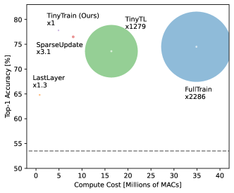
Figure 1 presents a comparison of our method’s performance with existing on-device training approaches. TinyTrain achieves the highest accuracy, with gains of 3.6-5.0% over fine-tuning the entire DNN, denoted by FullTrain. On the compute front, TinyTrain significantly reduces the memory footprint and computation required for backward pass by up to 2,286 $\times$ and 7.68 $\times$ , respectively. TinyTrain further outperforms the SOTA SparseUpdate method in all aspects, yielding: (a) 2.6-7.7% accuracy gain across nine datasets; (b) 2.4-3.1 $\times$ reduction in memory; and (c) 1.5-1.8 $\times$ lower computation costs. Finally, we demonstrate how our work makes important steps towards efficient training on very constrained edge devices by deploying TinyTrain on Raspberry Pi Zero 2 and Jetson Nano and showing that our multi-objective criterion can be efficiently computed within 20-35 seconds on both of our target edge devices (i.e. 3.4-3.8% of the total training time of TinyTrain), removing the necessity of offline search process of important layers and channels. Also, TinyTrain achieves an end-to-end on-device training in 10 minutes, an order of magnitude speedup over the two-hour training of FullTrain on Pi Zero 2. These findings open the door, for the first time, to performing on-device training with acceptable performance on a variety of resource-constrained devices, such as MCUs embedded in IoT frameworks.

2 Methodology

Problem Formulation. From a learning perspective, on-device DNN training at the extreme edge imposes unique characteristics that the model needs to address during deployment, primarily: (1) unseen target tasks with different data distributions (cross-domain), and (2) scarce labelled user data. To formally capture this setting, in this work, we cast it as a cross-domain few-shot learning (CDFSL) problem. In particular, we formulate it as K-way-N-shot learning [54] which allows us to accommodate more general scenarios instead of optimising towards one specific CDFSL setup (e.g. 5-way 5-shots). This formulation requires us to learn a DNN for $K$ classes given $N$ samples per class. To further push towards realistic scenarios, we learn one global DNN representation from various $K$ and $N$ , which can be used to learn novel tasks (see §3.1 and §A.1 for details).

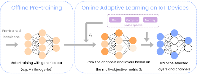
Our Pipeline. Figure 2 shows the processing flow of TinyTrain comprising two stages. The first stage is offline learning. By means of pre-training and meta-training, TinyTrain aims to find an informed weight initialisation, such that subsequently the model can be rapidly adapted to the user data with only a few samples (5-30), drastically reducing the burden of manual labelling and the overall training time compared to state of the art methods. The second stage is online learning. This stage takes place on the target edge device, where TinyTrain utilises its task-adaptive sparse-update method to selectively fine-tune the model using the limited user-specific, cross-domain target data, while minimising the memory and compute overhead.

2.1 Few-Shot Learning-Based Pre-training

The vast majority of existing on-device training pipelines optimise certain aspects of the system (i.e. memory or compute) via memory-saving techniques [6, 41, 58, 12] or fine-tuning a small set of layers/channels [4, 31, 45, 28, 43]. However, these methods neglect the aspect of sample efficiency in the low-data regime of tiny edge devices. As the availability of labelled data is severely limited at the extreme edge, existing on-device training approaches suffer from insufficient learning capabilities under such conditions.

In our work, we depart from the transfer-learning paradigm (i.e. DNN pre-training on source data, followed by fine-tuning on target data) of existing on-device training methods that are unsuitable to the very low data regime of edge devices. Building upon the insight of recent studies [17] that transfer learning does not reach a model’s maximum capacity on unseen tasks in the presence of only limited labelled data, we augment the offline stage of our training pipeline as follows. Starting from the pre-training of the DNN backbone using a large-scale public dataset, we introduce a subsequent meta-training process that meta-trains the pre-trained DNN given only a few samples (5-30) per class on simulated tasks in an episodic fashion. As shown in §3.3, this approach enables the resulting DNNs to perform more robustly and achieve higher accuracy when adapted to a target task despite the low number of examples, matching the needs of tiny edge devices. As a result, our few-shot learning (FSL)-based pre-training constitutes an important component to improve the attainable accuracy when only a few data samples are used for adaptation, reducing the training time while improving data and computation efficiency. Thus, TinyTrain alleviates the drawbacks of current work, by explicitly addressing the lack of labelled user data, and achieving faster training and lower accuracy loss.

Pre-training. For the backbones of our models, we employ feature extractors of different DNN architectures as in §3.1. These feature backbones are pre-trained with a large-scale image dataset, e.g. ImageNet [8].

Meta-training. For the meta-training phase, we employ the metric-based ProtoNet [50], which has been demonstrated to be simple and effective as an FSL method. ProtoNet computes the class centroids (i.e. prototypes) for a given support set and then performs nearest-centroid classification using the query set. Specifically, given a pre-trained feature backbone $f$ that maps inputs $x$ to an $m$ -dimensional feature space, ProtoNet first computes the prototypes $c_{k}$ for each class $k$ on the support set as $c_{k}=\frac{1}{N_{k}}\sum_{i:y_{i}=k}{f(x_{i})}$ , where $N_{k}=\sum_{i:y_{i}=k}1$ and $y$ are the labels. The probability of query set inputs $x$ for each class $k$ is then computed as:

p(y=k|x)=\frac{exp(-d(f(x),c_{k}))}{\sum_{j}exp(-d(f(x),c_{j}))}

(1)

We use cosine distance as the distance measure $d$ similarly to Hu et al. [17]. Note that ProtoNet enables the various-way-various-shot setting since the prototypes can be computed regardless of the number of ways and shots. Then, the feature backbones are meta-trained with MiniImageNet [56], a commonly used source dataset in CSFSL, to provide a weight initialisation that will be generalisable to multiple downstream tasks in the subsequent online stage (see §F.1 for the meta-training cost analysis).

2.2 Task-Adaptive Sparse Update

Existing FSL pipelines generally focus on data and sample efficiency and attend less to system optimisation [10, 50, 15, 54, 17], rendering most of these algorithms undeployable for the extreme edge, due to high computational and memory costs. In this context, sparse update [31, 43], which dictates that only a subset of essential layers and channels are to be trained, has emerged as a promising paradigm for making training feasible on resource-constrained devices.

Two key design decisions of sparse-update methods are i) the scheme for determining the sparse-update policy, i.e. which layers/channels should be fine-tuned, and ii) how often should the sparse-update policy be modified. In this context, a SOTA method, such as SparseUpdate [31], is characterised by important limitations. First, it casts the layer/channel selection as an optimisation problem that aims to maximise the accuracy gain subject to the memory constraints of the target device. However, as the optimisation problem is combinatorial, SparseUpdate solves it offline by means of a heuristic evolutionary algorithm that requires a few thousand trials. Secondly, as the search process for a good sparse-update policy is too expensive, it is practically infeasible to dynamically adjust the sparse-update policy whenever new target datasets are given, leading to performance degradation.

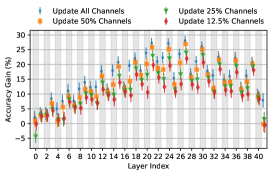
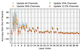
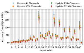
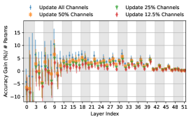
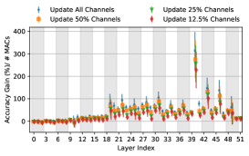
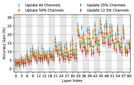
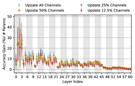
Multi-Objective Criterion. With resource constraints being at the forefront in tiny edge devices, we investigate the trade-offs among accuracy gain, compute and memory cost. To this end, we analyse each layer’s contribution (i.e. accuracy gain) on the target dataset by updating a single layer at a time, together with cost-normalised metrics, including accuracy gain per parameter and per MAC operation of each layer. Figure 3 shows the results of MCUNet [30] on the Traffic Sign [16] dataset (see §E.1 for more results). We make the following observations: (1) the peak point of accuracy gain occurs at the first layer of each block (pointwise convolutional layer) (Figure 3a), (2) the accuracy gain per parameter and computation cost occurs at the second layer of each block (depthwise convolutional layer) (Figures 3b and 3c). These findings indicate a non-trivial trade-off between accuracy, memory, and computation, demonstrating the necessity for an effective layer/channel selection method that jointly considers all the aspects.

To encompass both accuracy and efficiency aspects, we design a multi-objective criterion for the layer selection process of our task-adaptive sparse-update method. To quantify the importance of channels and layers on the fly, we propose the use of Fisher information on activations [1, 53, 23], often used to identify less important channels/layers for pruning [53, 55]. Whereas we use it as a proxy for more important channels/layers for weight update. Formally, given $N$ examples of target inputs, the Fisher information $\Delta_{o}$ can be calculated after backpropagating the loss $L$ with respect to activations $a$ of a layer:

\Delta_{o}=\frac{1}{2N}\sum_{n}^{N}(\sum_{d}^{D}a_{nd}g_{nd})^{2}

(2)

where gradient is denoted by $g_{nd}$ and $D$ is feature dimension of each channel (e.g. $D=H\times W$ of height $H$ and width $W$ ). We obtain the Fisher potential $P$ for a whole layer by summing $\Delta_{o}$ for all activation channels as: $P=\sum_{o}\Delta_{o}$ .

Having established the importance of channels in each layer, we define a new multi-objective metric $s$ that jointly captures importance, memory footprint and computational cost:

s_{i}=\frac{P_{i}}{\frac{\left\lVert W_{i}\right\rVert}{\underset{l\in\mathcal{L}}{\max}(\left\lVert W_{l}\right\rVert)}\times\frac{M_{i}}{\underset{l\in\mathcal{L}}{\max}(M_{l})}}

(3)

where $\left\lVert W_{i}\right\rVert$ and $M_{i}$ represent the number of parameters and multiply-accumulate (MAC) operations of the $i$ -th layer and are normalised by the respective maximum values $\underset{l\in\mathcal{L}}{\max}(\left\lVert W_{l}\right\rVert)$ and $\underset{l\in\mathcal{L}}{\max}(M_{l})$ across all layers $\mathcal{L}$ of the model. This multi-objective metric enables TinyTrain to rank different layers and prioritise the ones with higher Fisher potential per parameter and per MAC during layer selection. Further, as TinyTrain obtains multi-objective metric efficiently by running backpropagation only once for each target dataset, TinyTrain effectively alleviates the burdens of running the computationally heavy search processes a few thousand times.

Dynamic Layer/Channel Selection. We now present our dynamic layer/channel selection scheme, the second component of our task-adaptive sparse update, that runs at the online learning stage (i.e. deployment and meta-testing phase). Concretely, with reference to Algorithm 1, when a new on-device task needs to be learned (e.g. a new user or dataset), the sparse-update policy is modified to match its properties (lines 1-4). Contrary to the existing layer/channel selection approaches that remain fixed across tasks, our method is based on the key insight that different features/channels can play a more important role depending on the target dataset/task/user. As shown in §3.3, effectively tailoring the layer/channel selection to each task leads to superior accuracy compared to the pre-determined, static layer selection scheme of SparseUpdate, while further minimising system overheads.

As an initialisation step, TinyTrain is first provided with the memory and computation budget determined by hardware and users, e.g. 512 KB and 15% of total MACs can be given as backward-pass memory and computational budget. Then, we calculate the Fisher potential for each convolutional layer by performing backpropagation once using the given inputs of a target task (lines 1-2). Then, based on our multi-objective criterion (Eq. (3)) (line 3), we score each layer and progressively select as many layers as possible without violating the memory constraints (imposed by the peak memory usage of the model, optimiser, and activations memory) and resource budgets (imposed by users and target hardware) on an edge device (line 4).

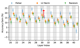
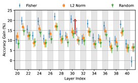
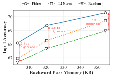
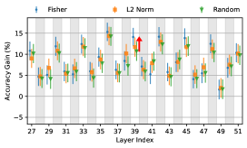
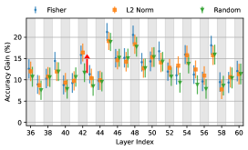
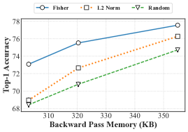
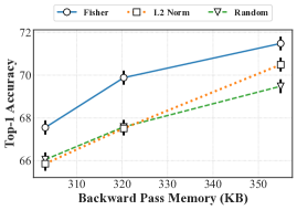
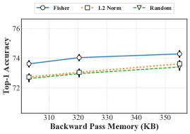
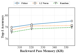
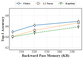
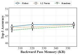
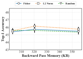
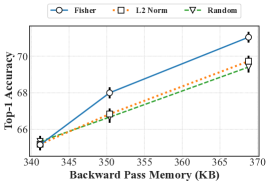
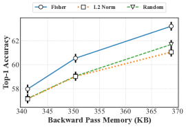
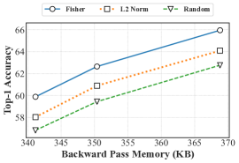
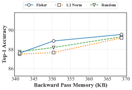
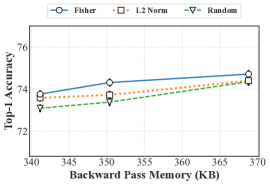
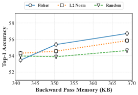
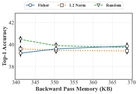
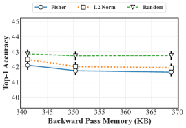
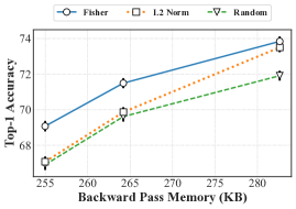
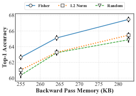
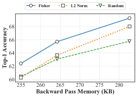
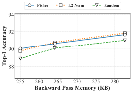
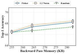
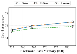
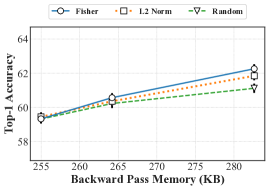
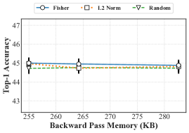
After having selected layers, within each selected layer, we identify the top- $K$ most important channels to update using the Fisher information for each activation channel, $\Delta_{o}$ , that was precomputed during the initialisation step (line 4). Note that the overhead of our dynamic layer/channel selection is minimal, which takes only 20-35 seconds on edge devices (more analysis in §3.2 and §3.3). Having finalised the layer/channel selection, we proceed with their sparse fine-tuning of the meta-trained DNN during meta-testing (see §C for detailed procedures). As in Figure 4 (MCUNet on Traffic Sign; refer to §E.5 for more results), dynamically identifying important channels for an update for each target task outperforms the static channel selections such as random- and L2-Norm-based selection.

Overall, the dynamic layer/channel selection scheme facilitates TinyTrain to achieve superior accuracy, while further minimising the memory and computation cost by co-optimising both system constraints, thereby enabling memory- and compute-efficient training at the extreme edge.

Require: Meta-trained backbone weights

W

, iterations

k

, Train data

D_{\text{train}}

, Test data

D_{\text{test}}

, memory and compute budgets

B_{\text{mem}}

B_{\text{compute}}

/* Dynamic layer/channel selection */

1 Compute the gradient using the given samples

D_{\text{train}}

2 Compute the Fisher potential using Eq. (2) from the Fisher information

4Compute our multi-objective metric

s

using Eq. (3)

6Perform the dynamic layer & channel selection using

\{W,s,B_{\text{mem}},B_{\text{compute}}\}

/* Perform sparse fine-tuning */

8 for $t=1,...,k$ do

9 Update the selected layers/channels using

D_{\text{train}}

11Evaluate the fine-tuned backbone using

D_{\text{test}}

Algorithm 1 Online learning stage of TinyTrain

3 Evaluation

3.1 Experimental Setup

We briefly explain our experimental setup in this subsection (refer to §A for further details).

Datasets. We use MiniImageNet [56] as the meta-train dataset, following the same setting as prior works on cross-domain FSL [17, 54, 13]. For meta-test datasets (i.e. target datasets of different domains than the source dataset of MiniImageNet), we employ all nine out-of-domain datasets of various domains from Meta-Dataset [54], excluding ImageNet because it is used to pre-train the models before deployment, making it an in-domain dataset. Extensive experimental results with nine different cross-domain datasets showcase the robustness and generality of our approach to the challenging CDFSL problem.

Architectures. Following Lin et al. [31], we employ three DNN architectures: MCUNet [30], MobileNetV2 [46], and ProxylessNAS [3]. These DNN models are pre-trained using ImageNet [8] and optimised for resource-limited IoT devices by adjusting the width multiplier.

Evaluation. To evaluate the CDFSL performance, we sample 200 tasks from the test split for each dataset. Then, we use testing accuracy on unseen samples of a new-domain target dataset. Following Triantafillou et al. [54], the number of classes and support/query sets are sampled uniformly at random regarding the dataset specifications. On the computational front, we present the computation cost in MAC operations and the peak memory footprint (i.e. the memory of the model parameters, optimisers and activations). We further measure latency and energy consumption when running end-to-end DNN training on actual edge devices.

Baselines. We compare TinyTrain with the following five baselines: (1) None does not perform any on-device training; (2) FullTrain [38] fine-tunes the entire model, representing a conventional transfer-learning approach; (3) LastLayer [45, 28] updates the last layer only; (4) TinyTL [4] updates the augmented lite-residual modules while freezing the backbone; and (5) SparseUpdate of MCUNetV3 [31], is a prior state-of-the-art (SOTA) method for on-device training that statically pre-determines which layers and channels to update before deployment and then updates them online.

Table 1: Top-1 accuracy results of TinyTrain and the baselines. TinyTrain achieves the highest accuracy with three DNN architectures on nine cross-domain datasets.

Model	Method	Traffic	Omniglot	Aircraft	Flower	CUB	DTD	QDraw	Fungi	COCO	Avg.
MCUNet	None	35.5	42.3	42.1	73.8	48.4	60.1	40.9	30.9	26.8	44.5
	FullTrain	82.0	72.7	75.3	90.7	66.4	74.6	64.0	40.4	36.0	66.9
	LastLayer	55.3	47.5	56.7	83.9	54.0	72.0	50.3	36.4	35.2	54.6
	TinyTL	78.9	73.6	74.4	88.6	60.9	73.3	67.2	41.1	36.9	66.1
	SparseUpdate	72.8	67.4	69.0	88.3	67.1	73.2	61.9	41.5	37.5	64.3
	TinyTrain (Ours)	79.3	73.8	78.8	93.3	69.9	76.0	67.3	45.5	39.4	69.3
	None	39.9	44.4	48.4	81.5	61.1	70.3	45.5	38.6	35.8	51.7
	FullTrain	75.5	69.1	68.9	84.4	61.8	71.3	60.6	37.7	35.1	62.7
Mobile	LastLayer	58.2	55.1	59.6	86.3	61.8	72.2	53.3	39.8	36.7	58.1
NetV2	TinyTL	71.3	69.0	68.1	85.9	57.2	70.9	62.5	38.2	36.3	62.1
	SparseUpdate	77.3	69.1	72.4	87.3	62.5	71.1	61.8	38.8	35.8	64.0
	TinyTrain (Ours)	77.4	68.1	74.1	91.6	64.3	74.9	60.6	40.8	39.1	65.6
	None	42.6	50.5	41.4	80.5	53.2	69.1	47.3	36.4	38.6	51.1
	FullTrain	78.4	73.3	71.4	86.3	64.5	71.7	63.8	38.9	37.2	65.0
Proxyless	LastLayer	57.1	58.8	52.7	85.5	56.1	72.9	53.0	38.6	38.7	57.0
NASNet	TinyTL	72.5	73.6	70.3	86.2	57.4	71.0	65.8	38.6	37.6	63.7
	SparseUpdate	76.0	72.4	71.2	87.8	62.1	71.7	64.1	39.6	37.1	64.7
	TinyTrain (Ours)	79.0	71.9	76.7	92.7	67.4	76.0	65.9	43.4	41.6	68.3

Table 2: Comparison of the memory footprint and computation costs for a backward pass between TinyTrain and the baselines.

Model	Method	Memory	Ratio	Compute	Ratio
MCUNet	FullTrain	950 MB	1,872 $\times$	44.9M	6.89 $\times$
	LastLayer	1.14 MB	2.3 $\times$	1.57M	0.23 $\times$
	TinyTL	569 MB	1,120 $\times$	26.4M	4.05 $\times$
	SparseUpdate	1.21 MB	2.4 $\times$	11.9M	1.82 $\times$
	TinyTrain (Ours)	0.51 MB	1 $\times$	6.51M	1 $\times$
	FullTrain	1,100 MB	2,286 $\times$	34.9M	7.12 $\times$
Mobile	LastLayer	0.61 MB	1.3 $\times$	0.80M	0.16 $\times$
NetV2	TinyTL	615 MB	1,279 $\times$	16.4M	3.35 $\times$
	SparseUpdate	1.47 MB	3.1 $\times$	8.10M	1.65 $\times$
	TinyTrain (Ours)	0.48 MB	1 $\times$	4.90M	1 $\times$
	FullTrain	899 MB	1,925 $\times$	38.4M	7.68 $\times$
Proxyless	LastLayer	0.45 MB	0.96 $\times$	0.59M	0.12 $\times$
NASNet	TinyTL	567 MB	1,214 $\times$	17.8M	3.57 $\times$
	SparseUpdate	1.34 MB	2.9 $\times$	7.60M	1.52 $\times$
	TinyTrain (Ours)	0.47 MB	1 $\times$	5.00M	1 $\times$

3.2 Main Results

Accuracy. Table 1 summarises accuracy results of TinyTrain and various baselines after adapting to cross-domain target datasets, averaged over 200 runs. We first observe that None attains the lowest accuracy among all baselines across all experiments, demonstrating the importance of on-device training when domain shift in train-test data distribution is present. LastLayer improves upon None with a marginal accuracy increase, suggesting that updating the last layer is insufficient to achieve high accuracy in cross-domain scenarios, likely due to final layer limits in the capacity. In addition, FullTrain, serving as a strong baseline as it assumes unlimited system resources, achieves high accuracy. TinyTL also yields moderate accuracy. However, as both FullTrain and TinyTL require prohibitively large memory and computation for training, they remain unsuitable to operate on resource-constrained devices, as shown below.

TinyTrain achieves the best accuracy on most datasets and the highest average accuracy across them, outperforming all the baselines including FullTrain, LastLayer, TinyTL, and SparseUpdate by 3.6-5.0 percentage points (pp), 13.0-26.9 pp, 4.8-7.2 pp, and 2.6-7.7 pp, respectively. This result indicates that our approach of identifying important parameters on the fly in a task-adaptive manner and updating them could be more effective in preventing overfitting given the few samples of CDFSL.

Memory and Compute. We investigate the memory and computation costs of on-device training by examining each method and DNN architecture. Table 2 shows how much additional memory and computation are required to perform training (backward pass) on top of inference (forward pass). We focus on the backward pass, as the objective of our work is to reduce the cost of the backward pass, which takes up the majority of the memory footprint of training [51]. Memory and computation of a forward pass can vary depending on the execution scheduling (e.g. patch-based inference).

We first observe that FullTrain and TinyTL consume significant amounts of memory, ranging between 899-1,100 MB and 567-615 MB, respectively, i.e. up to 2,286 $\times$ and 1,279 $\times$ more than TinyTrain, which exceeds the typical RAM size of IoT devices, such as Pi Zero (e.g. 512 MB). Note that a batch size of 100 is used for these two baselines as their accuracy degrades catastrophically with smaller batch sizes. Conversely, the other methods, including LastLayer, SparseUpdate, and TinyTrain, use a batch size of 1 and yield a smaller memory footprint and computational cost. Importantly, compared to SparseUpdate, TinyTrain enables on-device training with 2.4-3.1 $\times$ less memory and 1.52-1.82 $\times$ less computation. This gain can be attributed to the multi-objective criterion of TinyTrain’s sparse-update method, which co-optimises both memory and computation.

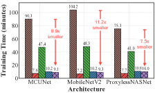
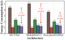
End-to-End Latency and Energy Consumption. We now examine the run-time system efficiency by measuring TinyTrain’s end-to-end training time and energy consumption, as shown in Figure 5. To this end, we deploy TinyTrain and the baselines on constrained edge devices, Pi Zero 2 and Jetson Nano. To measure the overall training cost, we include the time and energy consumption: (1) to load a pre-trained model, and (2) to perform training using all the samples (e.g. 25) for a certain number of iterations (e.g. 40), and (3) to perform dynamic layer/channel selection for task-adaptive sparse update (only for TinyTrain).

TinyTrain yields 1.08-1.12 $\times$ and 1.3-1.7 $\times$ faster on-device training than SOTA on Pi Zero 2 and Jetson Nano, respectively. Also, TinyTrain completes an end-to-end on-device training process within 10 minutes, an order of magnitude speedup over the two-hour training of conventional transfer learning, a.k.a. FullTrain on Pi Zero 2. Moreover, the latency of TinyTrain is shorter than all the baselines except for that of LastLayer which only updates the last layer but suffers from high accuracy loss. In addition, TinyTrain shows a significant reduction in the energy consumption (incurring 1.20-1.31kJ) compared to all the baselines, except for LastLayer, similarly to the latency results.

Summary. Our results demonstrate that TinyTrain can effectively learn cross-domain tasks requiring only a few samples, i.e. it generalises well to new samples and classes unseen during the offline learning phase. Furthermore, TinyTrain enables fast and energy-efficient on-device training on constrained IoT devices with significantly reduced memory footprint and computational load.

3.3 Ablation Study and Analysis

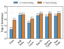
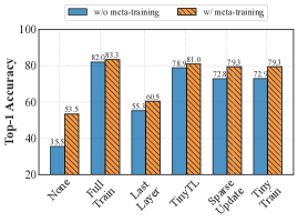
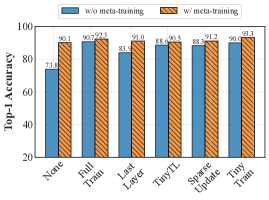
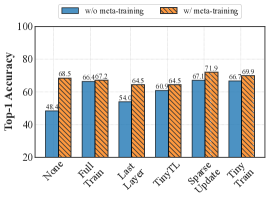
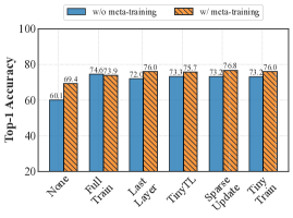
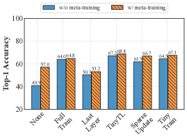
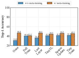
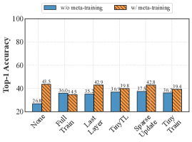
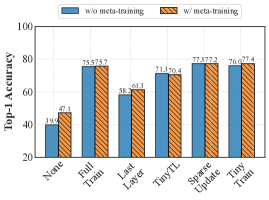
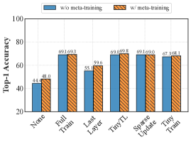
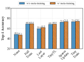
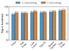
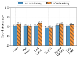
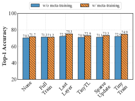
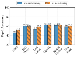
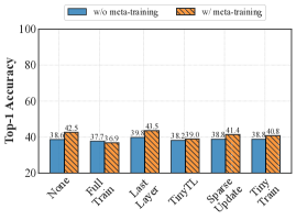
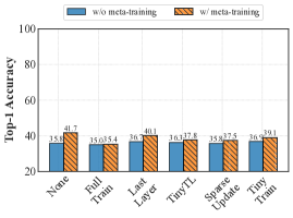
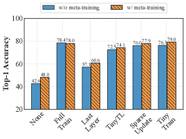
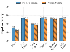
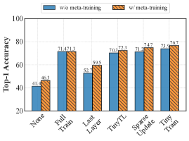
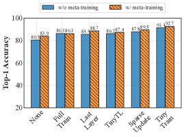
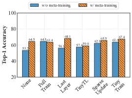
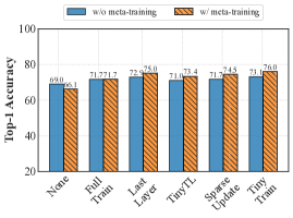
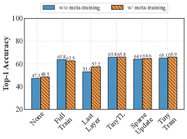
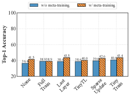
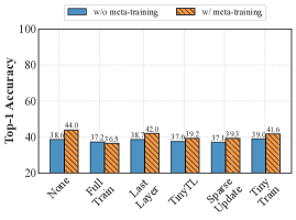
Impact of Meta-Training. We compare the accuracy between pre-trained DNNs with and without meta-training using MCUNet. Figure 6a shows that meta-training improves the accuracy by 0.6-31.8 pp over the DNNs without meta-training across all the methods (see §E.4 for more results). For TinyTrain, meta-training increases accuracy by 5.6 pp on average. This result shows the impact of meta-training compared to conventional transfer learning, demonstrating the effectiveness of our FSL-based pre-training (§2.1).

Robustness of Dynamic Channel Selection. We compare the accuracy of TinyTrain with and without dynamic channel selection, with the same set of layers to be updated within strict memory constraints using MCUNet. This comparison shows how much improvement is derived from dynamically selecting important channels based on our method at deployment time. Figure 6b shows that dynamic channel selection increases accuracy by 0.8-1.7 pp and 1.9-2.5 pp on average compared to static channel selection based on L2-Norm and Random, respectively (see §E.5 for more results). In addition, given a more limited memory budget, our dynamic channel selection maintains higher accuracy than static channel selection. Our ablation study reveals the robustness of the dynamic channel selection of our task-adaptive sparse-update (§2.2).

Efficiency of Task-Adaptive Sparse Update. Our dynamic layer/channel selection process takes around 20-35 seconds on our employed edge devices (i.e. Pi Zero 2 and Jetson Nano), accounting for only 3.4-3.8% of the total training time of TinyTrain. Note that our selection process is 30 $\times$ faster than SparseUpdate’s server-based evolutionary search, taking 10 minutes with abundant offline compute resources. This demonstrates the efficiency of our task-adaptive sparse update.

4 Related Work

On-Device Training. Driven by the increasing privacy concerns and the need for post-deployment adaptability to new tasks/users, the research community has recently turned its attention to enabling DNN training (i.e., backpropagation having forward and backward passes, and weights update) at the edge. First, researchers proposed memory-saving techniques to resolve the memory constraints of training [51, 5, 39, 9, 34]. For example, gradient checkpointing [6, 21, 24] discards activations of some layers in the forward pass and recomputes those activations in the backward pass. Microbatching [19] splits a minibatch into smaller subsets that are processed iteratively, to reduce the peak memory needs. Swapping [18, 57, 60] offloads activations or weights to an external memory/storage (e.g. from GPU to CPU or from an MCU to an SD card). Some works [41, 58, 12] proposed a hybrid approach by combining two or three memory-saving techniques. Although these methods reduce the memory footprint, they incur additional computation overhead on top of the already prohibitively expensive on-device training time at the edge. Instead, our work drastically minimises not only memory but also the amount of computation through its dynamic sparse update that identifies and trains on-the-fly only the most important layers/channels.

A few existing works [31, 4, 43] have also attempted to optimise both memory and computations, with prominent examples being TinyTL [4] and SparseUpdate [31]. However, TinyTL still demands excessive memory and computation (see §3.2). SparseUpdate suffers from accuracy loss, with a drop of 2.6-7.7% compared to TinyTrain) when on-device data are scarce, as at the extreme edge. In contrast, TinyTrain enables data-, compute-, and memory-efficient training on tiny edge devices by adopting FSL pre-training and dynamic layer/channel selection.

Cross-Domain Few-Shot Learning. Due to the scarcity of labelled user data on the device, developing Few-Shot Learning (FSL) techniques [15, 10, 2, 29, 50, 52, 47, 62] is a natural fit for on-device training. Also, a growing body of work focuses on cross-domain (out-of-domain) FSL (CDFSL) [13, 17, 54] where the source (meta-train) dataset drastically differs from the target (meta-test) dataset. CDFSL is practically relevant since in real-world deployment scenarios, the scarcely annotated target data (e.g. earth observation images [13, 54]) is often significantly different from the offline source data (e.g. (Mini-)ImageNet [56]). However, FSL-based methods only consider data efficiency, neglecting the memory and computation bottlenecks of on-device training. We explore joint optimisation of all the major bottlenecks of on-device training: data, memory, and computation.

5 Conclusion

We have developed the first realistic on-device training framework, TinyTrain, solving practical challenges in terms of data, memory, and compute constraints for extreme edge devices. TinyTrain meta-learns in a few-shot fashion during the offline learning stage and dynamically selects important layers and channels to update during deployment. As a result, TinyTrain outperforms all existing on-device training approaches by a large margin enabling, for the first time, fully on-device training on unseen tasks at the extreme edge. It allows applications to generalise to cross-domain tasks using only a few samples and adapt to the dynamics of the user devices and context.

Limitations & Societal Impacts. Our evaluation is currently limited to CNN-based architectures on vision tasks. As future work, we hope to extend TinyTrain to different architectures (e.g. Transformers, RNNs) and applications (e.g. audio or biological data). In addition, while on-device training avoids the excessive electricity consumption and carbon emissions of centralised training [49, 42], it has thus far been a significantly draining process for the battery life of edge devices. Nevertheless, TinyTrain paves the way towards alleviating this issue as demonstrated in Figure 5c.

References

Amari [1998] Shun-Ichi Amari. Natural gradient works efficiently in learning. Neural Computation, 10(2):251–276, 1998.
Antoniou et al. [2018] Antreas Antoniou, Harrison Edwards, and Amos Storkey. How to train your MAML. September 2018. URL https://openreview.net/forum?id=HJGven05Y7.
Cai et al. [2019] Han Cai, Ligeng Zhu, and Song Han. ProxylessNAS: Direct Neural Architecture Search on Target Task and Hardware. In International Conference on Learning Representations (ICLR), 2019.
Cai et al. [2020] Han Cai, Chuang Gan, Ligeng Zhu, and Song Han. TinyTL: Reduce Memory, Not Parameters for Efficient On-Device Learning. In Advances in Neural Information Processing Systems (NeurIPS), 2020.
Chen et al. [2021] Jianfei Chen, Lianmin Zheng, Zhewei Yao, Dequan Wang, Ion Stoica, Michael W Mahoney, and Joseph E Gonzalez. ActNN: Reducing Training Memory Footprint via 2-Bit Activation Compressed Training. In International Conference on Machine Learning (ICML), 2021.
Chen et al. [2016] Tianqi Chen, Bing Xu, Chiyuan Zhang, and Carlos Guestrin. Training Deep Nets with Sublinear Memory Cost, 2016. URL https://arxiv.org/abs/1604.06174.
Cimpoi et al. [2014] Mircea Cimpoi, Subhransu Maji, Iasonas Kokkinos, Sammy Mohamed, and Andrea Vedaldi. Describing Textures in the Wild. In IEEE Conference on Computer Vision and Pattern Recognition (CVPR), 2014.
Deng et al. [2009] Jia Deng, Wei Dong, Richard Socher, Li-Jia Li, Kai Li, and Li Fei-Fei. ImageNet: A Large-Scale Hierarchical Image Database. In IEEE Conference on Computer Vision and Pattern Recognition (CVPR), 2009.
Evans and Aamodt [2021] R David Evans and Tor Aamodt. AC-GC: Lossy Activation Compression with Guaranteed Convergence. In Advances in Neural Information Processing Systems (NeurIPS), 2021.
Finn et al. [2017] Chelsea Finn, Pieter Abbeel, and Sergey Levine. Model-Agnostic Meta-Learning for Fast Adaptation of Deep Networks. In International Conference on Machine Learning (ICML), 2017.
Gholami et al. [2018] Amir Gholami, Kiseok Kwon, Bichen Wu, Zizheng Tai, Xiangyu Yue, Peter Jin, Sicheng Zhao, and Kurt Keutzer. SqueezeNext: Hardware-Aware Neural Network Design. In IEEE Conference on Computer Vision and Pattern Recognition (CVPR), 2018.
Gim and Ko [2022] In Gim and JeongGil Ko. Memory-Efficient DNN Training on Mobile Devices. In Annual International Conference on Mobile Systems, Applications and Services (MobiSys), 2022.
Guo et al. [2020] Yunhui Guo, Noel C. Codella, Leonid Karlinsky, James V. Codella, John R. Smith, Kate Saenko, Tajana Rosing, and Rogerio Feris. A Broader Study of Cross-Domain Few-Shot Learning. In European Conference on Computer Vision (ECCV), 2020.
Han et al. [2016] Song Han, Huizi Mao, and William J. Dally. Deep Compression: Compressing Deep Neural Networks with Pruning, Trained Quantization and Huffman Coding. In International Conference on Learning Representations (ICLR), 2016.
Hospedales et al. [2022] Timothy Hospedales, Antreas Antoniou, Paul Micaelli, and Amos Storkey. Meta-Learning in Neural Networks: A Survey. IEEE Transactions on Pattern Analysis and Machine Intelligence (TPAMI), 44(9):5149–5169, 2022.
Houben et al. [2013] Sebastian Houben, Johannes Stallkamp, Jan Salmen, Marc Schlipsing, and Christian Igel. Detection of Traffic Signs in Real-World Images: The German Traffic Sign Detection Benchmark. In International Joint Conference on Neural Networks (IJCNN), 2013.
Hu et al. [2022] Shell Xu Hu, Da Li, Jan Stühmer, Minyoung Kim, and Timothy M. Hospedales. Pushing the limits of simple pipelines for few-shot learning: External data and fine-tuning make a difference. In IEEE Conference on Computer Vision and Pattern Recognition (CVPR), 2022.
Huang et al. [2020] Chien-Chin Huang, Gu Jin, and Jinyang Li. SwapAdvisor: Pushing Deep Learning Beyond the GPU Memory Limit via Smart Swapping. In International Conference on Architectural Support for Programming Languages and Operating Systems (ASPLOS), 2020.
Huang et al. [2019] Yanping Huang, Youlong Cheng, Ankur Bapna, Orhan Firat, Mia Xu Chen, Dehao Chen, HyoukJoong Lee, Jiquan Ngiam, Quoc V. Le, Yonghui Wu, and Zhifeng Chen. GPipe: Efficient Training of Giant Neural Networks Using Pipeline Parallelism. In International Conference on Neural Information Processing Systems (NeurIPS), 2019.
Jacob et al. [2018] Benoit Jacob, Skirmantas Kligys, Bo Chen, Menglong Zhu, Matthew Tang, Andrew Howard, Hartwig Adam, and Dmitry Kalenichenko. Quantization and Training of Neural Networks for Efficient Integer-Arithmetic-Only Inference. In IEEE Conference on Computer Vision and Pattern Recognition (CVPR), 2018.
Jain et al. [2020] Paras Jain, Ajay Jain, Aniruddha Nrusimha, Amir Gholami, Pieter Abbeel, Joseph Gonzalez, Kurt Keutzer, and Ion Stoica. Checkmate: Breaking the Memory Wall with Optimal Tensor Rematerialization. In Conference on Machine Learning and Systems (MLSys), 2020.
Jongejan et al. [2016] Jonas Jongejan, Henry Rowley, Takashi Kawashima, Jongmin Kim, and Nick Fox-Gieg. The quick, draw!-ai experiment. Mount View, CA, accessed Feb, 17(2018):4, 2016.
Kim et al. [2022] Minyoung Kim, Da Li, Shell X Hu, and Timothy Hospedales. Fisher SAM: Information Geometry and Sharpness Aware Minimisation. In International Conference on Machine Learning (ICML), 2022.
Kirisame et al. [2021] Marisa Kirisame, Steven Lyubomirsky, Altan Haan, Jennifer Brennan, Mike He, Jared Roesch, Tianqi Chen, and Zachary Tatlock. Dynamic Tensor Rematerialization. In International Conference on Learning Representations (ICLR), 2021.
Krishnamoorthi [2018] Raghuraman Krishnamoorthi. Quantizing Deep Convolutional Networks for Efficient Inference: A Whitepaper. arXiv:1806.08342 [cs, stat], 2018.
Krizhevsky et al. [2009] Alex Krizhevsky, Geoffrey Hinton, et al. Learning multiple layers of features from tiny images. 2009.
Lake et al. [2015] Brenden M. Lake, Ruslan Salakhutdinov, and Joshua B. Tenenbaum. Human-level Concept Learning through Probabilistic Program Induction. Science, 350(6266):1332–1338, 2015.
Lee and Nirjon [2020] Seulki Lee and Shahriar Nirjon. Learning in the Wild: When, How, and What to Learn for On-Device Dataset Adaptation. In International Workshop on Challenges in Artificial Intelligence and Machine Learning for Internet of Things (AIChallengeIoT), 2020.
Li et al. [2017] Zhenguo Li, Fengwei Zhou, Fei Chen, and Hang Li. Meta-SGD: Learning to Learn Quickly for Few-Shot Learning. arXiv:1707.09835 [cs], 2017.
Lin et al. [2020] Ji Lin, Wei-Ming Chen, Yujun Lin, John Cohn, Chuang Gan, and Song Han. MCUNet: Tiny Deep Learning on IoT Devices. In Advances in Neural Information Processing Systems (NeurIPS), 2020.
Lin et al. [2022] Ji Lin, Ligeng Zhu, Wei-Ming Chen, Wei-Chen Wang, Chuang Gan, and Song Han. On-Device Training Under 256KB Memory. In Advances on Neural Information Processing Systems (NeurIPS), 2022.
Lin et al. [2014] Tsung-Yi Lin, Michael Maire, Serge Belongie, James Hays, Pietro Perona, Deva Ramanan, Piotr Dollár, and C. Lawrence Zitnick. Microsoft COCO: Common Objects in Context. In European Conference on Computer Vision (ECCV), 2014.
Liu et al. [2020] Ning Liu, Xiaolong Ma, Zhiyuan Xu, Yanzhi Wang, Jian Tang, and Jieping Ye. AutoCompress: An Automatic DNN Structured Pruning Framework for Ultra-High Compression Rates. AAAI Conference on Artificial Intelligence (AAAI), 2020.
Liu et al. [2022] Xiaoxuan Liu, Lianmin Zheng, Dequan Wang, Yukuo Cen, Weize Chen, Xu Han, Jianfei Chen, Zhiyuan Liu, Jie Tang, Joey Gonzalez, Michael Mahoney, and Alvin Cheung. GACT: Activation Compressed Training for Generic Network Architectures. In International Conference on Machine Learning (ICML), 2022.
Ma et al. [2018] Ningning Ma, Xiangyu Zhang, Hai-Tao Zheng, and Jian Sun. ShuffleNet V2: Practical Guidelines for Efficient CNN Architecture Design. In European Conference on Computer Vision (ECCV), 2018.
Maji et al. [2013] Subhransu Maji, Esa Rahtu, Juho Kannala, Matthew B. Blaschko, and Andrea Vedaldi. Fine-grained visual classification of aircraft. CoRR, abs/1306.5151, 2013. URL http://arxiv.org/abs/1306.5151.
Nilsback and Zisserman [2008] Maria-Elena Nilsback and Andrew Zisserman. Automated Flower Classification over a Large Number of Classes. In Indian Conference on Computer Vision, Graphics & Image Processing (ICVGIP), 2008.
Pan and Yang [2010] Sinno Jialin Pan and Qiang Yang. A Survey on Transfer Learning. IEEE Transactions on Knowledge and Data Engineering (TKDE), 22(10):1345–1359, 2010.
Pan et al. [2021] Zizheng Pan, Peng Chen, Haoyu He, Jing Liu, Jianfei Cai, and Bohan Zhuang. Mesa: A Memory-saving Training Framework for Transformers. arXiv preprint arXiv:2111.11124, 2021.
Parisi et al. [2019] German I. Parisi, Ronald Kemker, Jose L. Part, Christopher Kanan, and Stefan Wermter. Continual Lifelong Learning with Neural Networks: A Review. Neural Networks, 113:54–71, 2019.
Patil et al. [2022] Shishir G Patil, Paras Jain, Prabal Dutta, Ion Stoica, and Joseph Gonzalez. POET: Training Neural Networks on Tiny Devices with Integrated Rematerialization and Paging. In International Conference on Machine Learning (ICML), 2022.
Patterson et al. [2022] David Patterson, Joseph Gonzalez, Urs Hölzle, Quoc Le, Chen Liang, Lluis-Miquel Munguia, Daniel Rothchild, David R So, Maud Texier, and Jeff Dean. The Carbon Footprint of Machine Learning Training Will Plateau, Then Shrink. Computer, 2022.
Profentzas et al. [2022] Christos Profentzas, Magnus Almgren, and Olaf Landsiedel. MiniLearn: On-Device Learning for Low-Power IoT Devices. In International Conference on Embedded Wireless Systems and Networks (EWSN, 2022.
Rastegari et al. [2016] Mohammad Rastegari, Vicente Ordonez, Joseph Redmon, and Ali Farhadi. XNOR-Net: ImageNet Classification Using Binary Convolutional Neural Networks. In European Conference on Computer Vision (ECCV), 2016.
Ren et al. [2021] Haoyu Ren, Darko Anicic, and Thomas A. Runkler. TinyOL: TinyML with Online-Learning on Microcontrollers. In International Joint Conference on Neural Networks (IJCNN), 2021.
Sandler et al. [2018] Mark Sandler, Andrew Howard, Menglong Zhu, Andrey Zhmoginov, and Liang-Chieh Chen. MobileNetV2: Inverted Residuals and Linear Bottlenecks. In IEEE/CVF Conference on Computer Vision and Pattern Recognition (CVPR), 2018.
Satorras and Estrach [2018] Victor Garcia Satorras and Joan Bruna Estrach. Few-Shot Learning with Graph Neural Networks. In International Conference on Learning Representations (ICLR), 2018.
Schroeder and Cui [2018] Brigit Schroeder and Yin Cui. Fgvcx fungi classification challenge 2018. Available online: github.com/visipedia/fgvcx_fungi_comp (accessed on 14 July 2021), 2018.
Schwartz et al. [2020] Roy Schwartz, Jesse Dodge, Noah A. Smith, and Oren Etzioni. Green AI. Commun. ACM, 63(12):54–63, 2020.
Snell et al. [2017] Jake Snell, Kevin Swersky, and Richard Zemel. Prototypical Networks for Few-shot Learning. In Advances in Neural Information Processing Systems (NeurIPS). 2017.
Sohoni et al. [2019] Nimit Sharad Sohoni, Christopher Richard Aberger, Megan Leszczynski, Jian Zhang, and Christopher Ré. Low-Memory Neural Network Training: A Technical Report. arXiv, 2019.
Sung et al. [2018] Flood Sung, Yongxin Yang, Li Zhang, Tao Xiang, Philip H. S. Torr, and Timothy M. Hospedales. Learning to Compare: Relation Network for Few-Shot Learning. In IEEE Conference on Computer Vision and Pattern Recognition (CVPR), 2018.
Theis et al. [2018] Lucas Theis, Iryna Korshunova, Alykhan Tejani, and Ferenc Huszár. Faster Gaze Prediction with Dense Networks and Fisher Pruning. arXiv, 2018.
Triantafillou et al. [2020] Eleni Triantafillou, Tyler Zhu, Vincent Dumoulin, Pascal Lamblin, Utku Evci, Kelvin Xu, Ross Goroshin, Carles Gelada, Kevin Swersky, Pierre-Antoine Manzagol, and Hugo Larochelle. Meta-Dataset: A Dataset of Datasets for Learning to Learn from Few Examples. In International Conference on Learning Representations (ICLR), 2020.
Turner et al. [2020] Jack Turner, Elliot J Crowley, Michael O’Boyle, Amos Storkey, and Gavin Gray. BlockSwap: Fisher-guided Block Substitution for Network Compression on a Budget. In International Conference on Learning Representations (ICLR), 2020.
Vinyals et al. [2016] Oriol Vinyals, Charles Blundell, Timothy Lillicrap, koray kavukcuoglu, and Daan Wierstra. Matching Networks for One Shot Learning. In Advances in Neural Information Processing Systems (NeurIPS). 2016.
Wang et al. [2018] Linnan Wang, Jinmian Ye, Yiyang Zhao, Wei Wu, Ang Li, Shuaiwen Leon Song, Zenglin Xu, and Tim Kraska. SuperNeurons: Dynamic GPU Memory Management for Training Deep Neural Networks. ACM SIGPLAN Notices, 53(1), 2018.
Wang et al. [2022] Qipeng Wang, Mengwei Xu, Chao Jin, Xinran Dong, Jinliang Yuan, Xin Jin, Gang Huang, Yunxin Liu, and Xuanzhe Liu. Melon: Breaking the Memory Wall for Resource-Efficient On-Device Machine Learning. In Annual International Conference on Mobile Systems, Applications and Services (MobiSys), 2022.
Welinder et al. [2011] P. Welinder, S. Branson, T. Mita, C. Wah, F. Schroff, S. Belongie, and P. Perona. Caltech-ucsd birds-200-2011 dataset. Technical Report Technical Report CNS-TR-2011-001, California Institute of Technology, 2011.
Wolf et al. [2020] Thomas Wolf, Lysandre Debut, Victor Sanh, Julien Chaumond, Clement Delangue, Anthony Moi, Pierric Cistac, Tim Rault, Remi Louf, Morgan Funtowicz, Joe Davison, Sam Shleifer, Patrick von Platen, Clara Ma, Yacine Jernite, Julien Plu, Canwen Xu, Teven Le Scao, Sylvain Gugger, Mariama Drame, Quentin Lhoest, and Alexander Rush. Transformers: State-of-the-Art Natural Language Processing. In Conference on Empirical Methods in Natural Language Processing: System Demonstrations (EMNLP), 2020.
Xu et al. [2022] Daliang Xu, Mengwei Xu, Qipeng Wang, Shangguang Wang, Yun Ma, Kang Huang, Gang Huang, Xin Jin, and Xuanzhe Liu. Mandheling: Mixed-Precision On-Device DNN Training with DSP Offloading. In Annual International Conference on Mobile Computing And Networking (MobiCom), 2022.
Zhang et al. [2021] Xueting Zhang, Debin Meng, Henry Gouk, and Timothy M. Hospedales. Shallow Bayesian Meta Learning for Real-World Few-Shot Recognition. In IEEE/CVF International Conference on Computer Vision (ICCV), 2021.

Supplementary Material
TinyTrain: Deep Neural Network Training at the Extreme Edge

\doparttoc\faketableofcontents

\parttoc

Appendix A Detailed Experimental Setup

This section provides additional information on the experimental setup.

A.1 Datasets

Following the conventional setup for evaluating cross-domain FSL performances on MetaDataset in prior arts [17, 54, 13], we use MiniImageNet [56] for Meta-Train and the non-ILSVRC datasets in MetaDataset [54] for Meta-Test. Specifically, MiniImageNet contains 100 classes from ImageNet-1k, split into 64 training, 16 validation, and 20 testing classes. The resolution of the images is downsampled to 84 $\times$ 84. The MetaDataset used as Meta-Test datasets consists of nine public image datasets from a variety of domains, namely Traffic Sign [16], Omniglot [27], Aircraft [36], Flowers [37], CUB [59], DTD [7], QDraw [22], Fungi [48], and COCO [32]. Note that the ImageNet dataset is excluded as it is already used for pre-training the models during the meta-training phase, which makes it an in-domain dataset. We showcase the robustness and generality of our approach to the challenging cross-domain few-shot learning (CDFSL) problem via extensive evaluation of these datasets. The details of each target dataset employed in our study are described below.

The Traffic Sign [16] dataset consists of 50,000 images out of 43 classes regarding German road signs.

The Omniglot [27] dataset has 1,623 handwritten characters (i.e. classes) from 50 different alphabets. Each class contains 20 examples.

The Aircraft [36] dataset contains images of 102 model variants with 100 images per class.

The VGG Flowers (Flower) [37] dataset is comprised of natural images of 102 flower categories. The number of images in each class ranges from 40 to 258.

The CUB-200-2011 (CUB) [59] dataset is based on the fine-grained classification of 200 different bird species.

The Describable Textures (DTD) [7] dataset comprises 5,640 images organised according to a list of 47 texture categories (classes) inspired by human perception.

The Quick Draw (QDraw) [22] is a dataset consisting of 50 million black-and-white drawings of 345 categories (classes), contributed by players of the game Quick, Draw!

The Fungi [48] dataset is comprised of around 100K images of 1,394 wild mushroom species, each forming a class.

The MSCOCO (COCO) [32] dataset is the train2017 split of the COCO dataset. COCO contains images from Flickr with 1.5 million object instances of 80 classes.

A.2 Model Architectures

Following [31], we employ optimised DNN architectures designed to be used in resource-limited IoT devices, including MCUNet [30], MobileNetV2 [46], and ProxylessNASNet [3]. The DNN models are pre-trained using ImageNet [8]. Specifically, the backbones of MCUNet (using the 5FPS ImageNet model), MobileNetV2 (with the 0.35 width multiplier), and ProxylessNAS (with a width multiplier of 0.3) have 23M, 17M, 19M MACs and 0.48M, 0.25M, 0.33M parameters, respectively. Note that MACs are calculated based on an input resolution of $128\times 128$ with an input channel dimension of 3. The basic statistics of the three DNN architectures are summarised in Table 3.

Table 3: The statistics of our employed DNN architectures.

Model	Param	MAC	# Layers	# Blocks
MCUNet	0.46M	22.5M	42	13
MobileNetV2	0.29M	17.4M	52	17
ProxylessNASNet	0.36M	19.2M	61	20

A.3 Training Details

We adopt a common training strategy to meta-train the pre-trained DNN backbones, which helps us avoid over-engineering the training process for each dataset and architecture [17]. Specifically, we meta-train the backbone for 100 epochs. Each epoch has 2000 episodes/tasks. A warm-up and learning rate scheduling with cosine annealing are used. The learning rate increases from $10^{-6}$ to $5\times 10^{-5}$ in 5 epochs. Then, it decreases to $10^{-6}$ . We use SGD with momentum as an optimiser.

A.4 Details for Evaluation Setup

To evaluate the cross-domain few-shot classification performance, we sample 200 different tasks from the test split for each dataset. Then, as key performance metrics, we first use testing accuracy on unseen samples of a new domain as the target dataset. Note that the number of classes and support/query sets are sampled uniformly at random based on the dataset specifications. In addition, we analytically calculate the computation cost and memory footprint required for the forward pass and backward pass (i.e. model parameters, optimisers, activations). More specifically, for the memory footprint for the backward pass, we include (1) model memory for the weights to be updated, (2) optimiser memory for gradients, and (3) activations memory for intermediate outputs for weights update. Also, we measure latency and energy consumption to perform end-to-end training of a deployed DNN on the edge device. We deploy TinyTrain and the baselines on a tiny edge device, Pi Zero. To measure the end-to-end training time and energy consumption, we include the time and energy used to: (1) load a pre-trained model, (2) perform training using all the samples (e.g. 25) for a certain number of iterations (e.g. 40). For TinyTrain, we also include the time and energy to conduct a dynamic layer/ channel selection based on our proposed importance metric, by computing the Fisher information on top of those to load a model and fine-tune it. Regarding energy, we measure the total amount of energy consumed by a device during the end-to-end training process. This is performed by measuring the power consumption on Pi Zero using a YOTINO USB power meter and deriving the energy consumption following the equation: Energy = Power $\times$ Time.

A.5 Baselines

We include the following baselines in our experiments to evaluate the effectiveness of TinyTrain.

None. This baseline does not perform any on-device training during deployment. Hence, it shows the accuracy drops of the DNNs when the model encounters a new task of a cross-domain dataset.

FullTrain. This method trains the entire backbone, serving as the strong baseline in terms of accuracy performance, as it utilises all the required resources without system constraints. However, this method intrinsically consumes the largest amount of system resources in terms of memory and computation among all baselines.

LastLayer. This refers to adapting only the head (i.e. the last layer or classifier), which requires relatively small memory footprint and computation. However, its accuracy typically is too low to be practical. Prior works [45, 28] adopt this method to update the last layer only for on-device training.

TinyTL [4]. This method proposes to add a small convolutional block, named the lite-residual module, to each convolutional block of the backbone network. During training, TinyTL updates the lite-residual modules while freezing the original backbone, requiring less memory and fewer computations than training the entire backbone. As shown in our results, TinyTrain requires the second largest amount of memory and compute resources among all baselines.

SparseUpdate [31]. This method reduces the memory footprint and computation in performing on-device training. Memory reduction comes from updating selected layers in the network, followed by another selection of channels within the selected layers. However, SparseUpdate adopts a static channel and layer selection policy that relies on evolutionary search (ES). This ES-based selection scheme requires compute and memory resources that the extreme-edge devices can not afford. Even in the offline compute setting, it takes around 10 mins to complete the search.

Appendix B Details of Sampling Algorithm during Meta-Testing

B.1 Sampling Algorithm during Meta-Testing

We now describe the sampling algorithm during meta-testing that produces realistically imbalanced episodes of various ways and shots (i.e. K-way-N-shot), following Triantafillou et al. [54]. The sampling algorithm is designed to accommodate realistic deployment scenarios by supporting the various-way-various-shot setting. Given a data split (e.g. train, validation, or test split) of the dataset, the overall procedure of the sampling algorithm is as follows: (1) sample of a set of classes $\mathcal{C}$ and (2) sample support and query examples from $\mathcal{C}$ .

Sampling a set of classes. First of all, we sample a certain number of classes from the given split of a dataset. The ‘way’ is sampled uniformly from the pre-defined range [5, MAX], where MAX indicates either the maximum number of classes or 50. Then, ‘way’ many classes are sampled uniformly at random from the given split of the dataset. For datasets with a known class organisation, such as ImageNet and Omniglot, the class sampling algorithm differs as described in [54].

Sampling support and query examples. Having selected a set of classes, we sample support and query examples by following the principle that aims to simulate realistic scenarios with limited (i.e. few-shot) and imbalanced (i.e. realistic) support set sizes as well as to achieve a fair evaluation of our system via query set.

•

Support Set Size. Based on the selected set of classes from the first step (i.e. sampling a set of classes), the support set is at most 100 (excluding the query set described below). The support set size is at least one so that every class has at least one image. The sum of support set sizes across all the classes is capped at 500 examples as we want to consider few-shot learning (FSL) in the problem formulation.
•

Shot of each class. After having determined the support set size, we now obtain the ‘shot’ of each class.
•

Query Set Size. We sample a class-balanced query set as we aim to perform well on all classes of samples. The number of minimum query sets is capped at 10 images per class.

B.2 Sample Statistics during Meta-Testing

In this subsection, we present summary statistics regarding the support and query sets based on the sampling algorithm described above in our experiments. In our evaluation, we conducted 200 trials of experiments (200 sets of support and query samples) for each target dataset. Table 4 shows the average (Avg.) number of ways, samples, and shots of each dataset as well as their standard deviations (SD), demonstrating that the sampled target data are designed to be the challenging and realistic various-way-various-shot CDFSL problem. Also, as our system performs well on such challenging problems, we demonstrate the effectiveness of our system.

Table 4: The summary statistics of the support and query sets sampled from nine cross-domain datasets.

	Traffic	Omniglot	Aircraft	Flower	CUB	DTD	QDraw	Fungi	COCO
Avg. Num of Ways	22.5	19.3	9.96	9.5	15.6	6.2	27.3	27.2	21.8
Avg. Num of Samples (Support Set)	445.9	93.7	369.4	287.8	296.3	324.0	460.0	354.7	424.1
Avg. Num of Samples (Query Set)	224.8	193.4	99.6	95.0	156.4	61.8	273.0	105.5	217.8
Avg. Num of Shots (Support Set)	29.0	4.6	38.8	30.7	20.7	53.3	23.6	15.6	27.9
Avg. Num of Shots (Query Set)	10	10	10	10	10	10	10	10	10
SD of Num of Ways	11.8	10.8	3.4	3.1	6.6	0.8	13.2	14.4	11.5
SD of Num of Samples (Support Set)	90.6	81.2	135.9	159.3	152.4	148.7	94.8	158.7	104.9
SD of Num of Samples (Query Set)	117.7	108.1	34.4	30.7	65.9	8.2	132.4	51.8	114.8
SD of Num of Shots (Support Set)	21.9	2.4	14.9	14.9	10.5	24.5	17.0	8.9	20.7
SD of Num of Shots (Query Set)	0.0	0.0	0.0	0.0	0.0	0.0	0.0	0.0	0.0
Num of Trials	200	200	200	200	200	200	200	200	200

Appendix C Fine-tuning Procedure during Meta-Testing

As we tackle realistic and challenging scenarios of the cross-domain few-shot learning (CDFSL) problem, the pre-trained DNNs can encounter a target dataset drawn from an unseen domain, where the pre-trained DNNs could fail to generalise due to a considerable shift in the data distribution.

Hence, to adjust to the target data distribution, we perform fine-tuning (on-device training) on the pre-trained DNNs by a few gradient steps while leveraging the data augmentation (as explained below). Specifically, the feature backbone as the DNNs is fine-tuned as our employed models are based on ProtoNet.

Our fine-tuning procedure during the meta-testing phase is similar to that of [13, 17]. First of all, as the support set is the only labelled data during meta-testing, prior work [13] fine-tunes the models using only the support set. For [17], it first uses data augmentation with the given support set to create a pseudo query set. After that, it uses the support set to generate prototypes and the pseudo query set to perform backpropagation using Eq. 1. Differently from [13],the fine-tuning procedure of [17] does not need to compute prototypes and gradients using the same support set using Eq. 1. However, Hu et al. [17] simply fine-tune the entire DNNs without memory-and compute-efficient on-device training techniques, which becomes one of our baselines, FullTrain requiring prohibitively large memory footprint and computation costs to be done on-device during deployment. In our work, for all the on-device training methods including TinyTrain, we adopt the fine-tuning procedure introduced in [17]. However, we extend the vanilla fine-tuning procedure with existing on-device training methods (i.e. LastLayer, TinyTL, SparseUpdate, which serve as the baselines of on-device training in our work) so as to improve the efficiency of on-device training on the extremely resource-constrained devices. Furthermore, our system, TinyTrain, not only extends the fine-tuning procedure with memory-and compute-efficient on-device training but also proposes to leverage data-efficient FSL pretraining to enable the first data-, memory-, and compute-efficient on-device training framework on edge devices.

Appendix D System Implementation

The offline component of our system is built on top of PyTorch (version 1.10) and runs on a Linux server equipped with an Intel Xeon Gold 5218 CPU and NVIDIA Quadro RTX 8000 GPU. This component is used to obtain the pre-trained model weights, i.e. pre-training and meta-training. Then, the online component of our system is implemented and evaluated on Raspberry Pi Zero 2 and NVIDIA Jetson Nano, which constitute widely used and representative embedded platforms. Pi Zero 2 is equipped with a quad-core 64-bit ARM Cortex-A53 and limited 512 MB RAM. Jetson Nano has a quad-core ARM Cortex-A57 processor with 4 GB of RAM. Also, we do not use sophisticated memory optimisation methods or compiler directives between the inference layer and the hardware to decrease the peak memory footprint; such mechanisms are orthogonal to our algorithmic innovation and may provide further memory reduction on top of our task-adaptive sparse update.

Appendix E Additional Results

In this section, we present additional results that are not included in the main content of the paper due to the page limit.

E.1 Memory- and Compute-aware Analysis

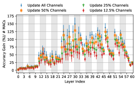
In §2.2, to investigate the trade-offs among accuracy gain, compute and memory cost, we analysed each layer’s contribution (i.e. accuracy gain) on the target dataset by updating a single layer at a time, together with cost-normalised metrics, including accuracy gain per parameter and per MAC operation of each layer. MCUNet is used as a case study. Hence, here we provide the results of memory- and compute-aware analysis on the remaining architectures (MobileNetV2 and ProxylessNASNet) based on the Traffic Sign dataset as shown in Figure 7 and 8.

The observations on MobileNetV2 and ProxylessNASNet are similar to those of MCUNet. Specifically: (a) accuracy gain per layer is generally highest on the first layer of each block for both MobileNetV2 and ProxylessNASNet; (b) accuracy gain per parameter of each layer is higher on the second layer of each block for both MobileNetV3 and ProxylessNASNet, but it is not a clear pattern; and (c) accuracy gain per MACs of each layer has peaked on the second layer of each block for MobileNetV2, whereas it does not have clear patterns for ProxylessNASNet. These observations indicate a non-trivial trade-off between accuracy, memory, and computation for all the employed architectures in our work.

E.2 Pairwise Comparison among Different Channel Selection Schemes

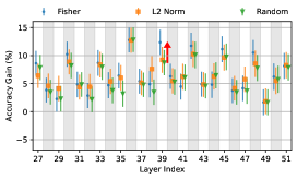
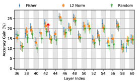
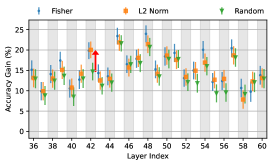
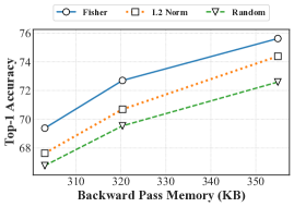
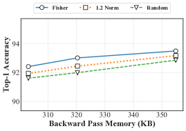
Here, we present additional results regarding the pairwise comparison between our dynamic channel selection and static channel selections (i.e. Random and L2-Norm). Figure 9 and 10 show that the results of MobileNetV2 and ProxylessNASNet on the Traffic Sign dataset, respectively.

Similar to the results of MCUNet, the dynamic channel selection on MobileNetV2 and ProxylessNASNet consistently outperforms static channel selections as the accuracy gain per layer differs by up to 5.1%. Also, the gap between dynamic and static channel selection increases as fewer channels are selected for updates.

E.3 End-to-End Latency Breakdown of TinyTrain and SparseUpdate

In this subsection, we present the end-to-end latency breakdown to highlight the efficiency of our task-adaptive sparse update (i.e. the dynamic layer/channel selection process during deployment) by comparing our work (TinyTrain) with previous SOTA (SparseUpdate). We present the time to identify important layers/channels by calculating Fisher Potential (i.e. Fisher Calculation in Table 5 and 6) and the time to perform on-device training by loading a pre-trained model and performing backpropagation (i.e. Run Time in Tables 5 and 6).

In addition to the main results of on-device measurement on Pi Zero 2 presented in §3.2, we selected Jetson Nano as an additional device and performed experiments in order to ensure that our results regarding system efficiency are robust and generalisable across diverse and realistic devices. We used the same experimental setup (as detailed in §3.1 and §A.4) as the one used for Pi Zero 2.

As shown in Table 5 and 6, our experiments show that TinyTrain enables efficient on-device training, outperforming SparseUpdate by 1.3-1.7 $\times$ on Jetson Nano and by 1.08-1.12 $\times$ on Pi Zero 2 with respect to end-to-end latency. Moreover, Our dynamic layer/channel selection process takes around 18.7-35.0 seconds on our employed edge devices (i.e. Jetson Nano and Pi Zero 2), accounting for only 3.4-3.8% of the total training time of TinyTrain.

Table 5: The end-to-end latency breakdown of TinyTrain and SOTA on Pi Zero 2. The end-to-end latency includes time (1) to load a pre-trained model, (2) to perform training using given samples (e.g. 25) over 40 iterations, and (3) to calculate fisher information on activation (For TinyTrain).

Model	Method	Fisher Calculation (s)	Run Time (s)	Total (s)	Ratio
MCUNet	SparseUpdate	0.0	607	607	1.12 $\times$
MCUNet	TinyTrain (Ours)	18.7	526	544	1 $\times$
MobileNetV2	SparseUpdate	0.0	611	611	1.10 $\times$
MobileNetV2	TinyTrain (Ours)	20.1	536	556	1 $\times$
ProxylessNASNet	SparseUpdate	0.0	645	645	1.08 $\times$
ProxylessNASNet	TinyTrain (Ours)	22.6	575	598	1 $\times$

Table 6: The end-to-end latency breakdown of TinyTrain and SOTA on Jetson Nano. The end-to-end latency includes time (1) to load a pre-trained model, (2) to perform training using given samples (e.g., 25) over 40 iterations, and (3) to calculate fisher information on activation (For TinyTrain).

Model	Method	Fisher Calculation (s)	Run Time (s)	Total (s)	Ratio
MCUNet	SparseUpdate	0.0	1,189	1,189	1.3 $\times$
MCUNet	TinyTrain (Ours)	35.0	892	927	1 $\times$
MobileNetV2	SparseUpdate	0.0	1,282	1,282	1.5 $\times$
MobileNetV2	TinyTrain (Ours)	32.2	815	847	1 $\times$
ProxylessNASNet	SparseUpdate	0.0	1,517	1,517	1.7 $\times$
ProxylessNASNet	TinyTrain (Ours)	26.8	869	896	1 $\times$

E.4 Impact of Meta-Training

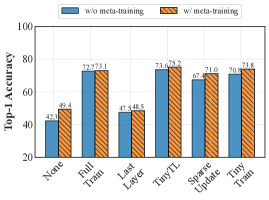
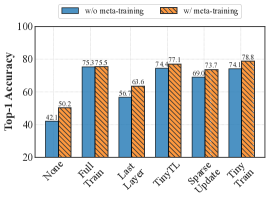
In this subsection, we present the complete results of the impact of meta-training. As discussed in §3.3, Figure 6a shows the average Top-1 accuracy with and without meta-training using MCUNet over nine cross-domain datasets. This analysis shows the impact of meta-training compared to conventional transfer learning, demonstrating the effectiveness of our FSL-based pre-training. However, it does not reveal the accuracy results of individual datasets and models. Hence, in this subsection, we present figures that compare Top-1 accuracy with and without meta-training for each architecture and dataset with all the on-device training methods to present the complete results of the impact of meta-training. Figures 11, 12, and 13 demonstrate the effect of meta-training based on MCUNet, MobileNetV2, and ProxylessNASNet, respectively, across all the on-device training methods and nine cross-domain datasets.

E.5 Robustness of Dynamic Channel Selection

As described in §3.3, to show how much improvement is derived from dynamically selecting important channels based on our method at deployment time, Figure 6b compares the accuracy of TinyTrain with and without dynamic channel selection, with the same set of layers to be updated within strict memory constraints using MCUNet. In this subsection, we present the full results regarding the robustness of our dynamic channel selection scheme using all the employed architectures and cross-domain datasets. Figures 14, 15, and 16 demonstrate the robustness of dynamic channel selection using MCUNet, MobileNetV2, and ProxylessNASNet, respectively, based on nine cross-domain datasets. Note that the reported results are averaged over 200 trials, and 95% confidence intervals are depicted.

Appendix F Further Analysis and Discussion

F.1 Cost of Meta-Training

In this subsection, we analyse the cost of meta-training, one of the major components of our FSL-based pre-training, in terms of the overall latency to perform meta-training. In our experiments, the offline meta-training on the source dataset, MiniImageNet, takes 5-6 hours across three architectures. However, note that the cost is small as meta-training needs to be performed only once per architecture. Furthermore, this cost is amortised by being able to reuse the same resulting meta-trained model across multiple downstream tasks (different target datasets) and devices, e.g. Raspberry Pi Zero 2 and Jetson Nano.

Appendix G Extended Related Work

G.1 On-Device Training

Scarce memory and compute resources are major bottlenecks in deploying DNNs on tiny edge devices. In this context, researchers have largely focused on optimising the inference stage (i.e. forward pass) by proposing lightweight DNN architectures [11, 46, 35], pruning [14, 33], and quantisation methods [20, 25, 44], leveraging the inherent redundancy in weights and activations of DNNs. Driven by the increasing privacy concerns and the need for post-deployment adaptability to new tasks or users, the research community has recently turned its attention to enabling DNN training (i.e., backpropagation having both forward and backward passes, and weights update) at the edge.

Researchers proposed memory-saving techniques to resolve the memory constraints of training [51, 5, 39, 9, 34]. For example, gradient checkpointing [6, 21, 24] discards activations of some layers in the forward pass and recomputes those activations in the backward pass. Microbatching [19] splits a minibatch into smaller subsets that are processed iteratively, to reduce the peak memory needs. Swapping [18, 57, 60] offloads activations or weights to an external memory/storage (e.g. from GPU to CPU or from an MCU to an SD card). Some works [41, 58, 12] proposed a hybrid approach by combining two or three memory-saving techniques. Although these methods reduce the memory footprint, they incur additional computation overhead on top of the already prohibitively expensive on-device training time at the edge. Instead, TinyTrain drastically minimises not only memory but also the amount of computation through its dynamic sparse update that identifies and trains only the most important layers/channels on-the-fly.

A few existing works [31, 4, 43] have also attempted to optimise both memory and computations, with prominent examples being TinyTL [4] and SparseUpdate [31]. By selectively updating only a subset of layers and channels during on-device training, these methods effectively reduce both the memory and computation load. Nonetheless, as shown in §3.2, the performance of this approach drops dramatically (up to 7.7% for SparseUpdate) when applied at the extreme edge where data availability is low. This occurs because the approach requires access to the entire target dataset (e.g. SparseUpdate [31] uses the entire CIFAR-100 dataset [26]), which is unrealistic for such devices in the wild. More importantly, it requires a large number of epochs (e.g. SparseUpdate requires 50 epochs) to reach high accuracy, which results in an excessive training time of up to 10 days when deployed on extreme edge devices, such as STM32F746 MCUs. Also, these methods require running a few thousands of computationally heavy search [31] or pruning [43] processes on powerful GPUs to identify important layers/channels for each target dataset; as such, the current static layer/channel selection scheme cannot be adapted on-device to match the properties of the user data and hence remains fixed after deployment, leading to an accuracy drop. In addition, TinyTL still demands excessive memory and computation (see §3.2). In contrast, TinyTrain enables data-, compute-, and memory-efficient training on tiny edge devices by adopting few-shot learning pre-training and dynamic layer/channel selection.

G.2 Few-Shot Learning

Due to the scarcity of labelled user data on the device, developing Few-Shot Learning (FSL) techniques is a natural fit for on-device training [15]. FSL methods aim to learn a target task given a few examples (e.g. 5-30 samples per class) by transferring the knowledge from large source data (i.e. meta-training) to scarcely annotated target data (i.e. meta-testing). Until now, several FSL schemes have been proposed, ranging from gradient-based [10, 2, 29], and metric-based [50, 52, 47] to Bayesian-based [62]. Recently, a growing body of work has been focusing on cross-domain (out-of-domain) FSL (CDFSL) [13]. The CDFSL setting dictates that the source (meta-train) dataset drastically differs from the target (meta-test) dataset. As such, although CDFSL is more challenging than the standard in-domain (i.e. within-domain) FSL [17], it tackles more realistic scenarios, which are similar to the real-world deployment scenarios targeted by our work. In our work, we focus on realistic use-cases where the available source data (e.g. MiniImageNet [56]) are significantly different from target data (e.g. meta-dataset [54]) with a few samples (5-30 samples per class), and hence incorporate CDFSL techniques into TinyTrain.

FSL-based methods only consider data efficiency and neglect the memory and computation bottlenecks of on-device training. Therefore, we explore joint optimisation of three major pillars of on-device training such as data, memory, and computation.