LTL Synthesis on Infinite-State Arenas defined by Programs

Abstract.

This paper deals with the problem of automatically and correctly controlling infinite-state reactive programs to achieve LTL goals. Applications include adapting a program to new requirements, or to repair bugs discovered in the original specification or program code. Existing approaches are able to solve this problem for safety and some reachability properties, but require an a priori template of the solution for more general properties. Fully automated approaches for full LTL exist, reducing the problem into successive finite LTL reactive synthesis problems in an abstraction-refinement loop. However, they do not terminate when the number of steps to be completed depends on unbounded variables. Our main insight is that safety abstractions of the program are not enough — fairness properties are also essential to be able to decide many interesting problems, something missed by existing automated approaches. We thus go beyond the state-of-the-art to allow for automated reactive program control for full LTL, with automated discovery of the knowledge, including fairness, of the program needed to determine realisability. We further implement the approach in a tool, with an associated DSL for reactive programs, and illustrate the approach through several case studies.

1. Introduction

Reactive synthesis is the problem of determining whether a specification is realisable in the context of some adversarial environment. When realisable, there is a controller that reacts to the environment appropriately to force satisfaction of the specification. Dually, when unrealisable, the environment has a counter strategy to force violation of the specification. Essentially, this corresponds to a game over the specification. The focus of this paper is on synthesis for program control, where in addition we are given a (reactive) program which acts as the game arena, which the controller must navigate to achieve the specification. However, the state of a program is captured by the value of its possibly arbitrarily-valued variables, and identifying updates to these that could be relevant to realisability of a specification is not easy, given the infinite-state space.

As with many infinite-state problems, synthesis over infinite-state spaces is undecidable in general. However, methods to approach this problem have gained some attention in recent years. These methods build and focus on finite abstractions of the state space, as standard for infinite-state problems. When counterexamples show that the abstraction is not accurate enough to determine realisability, they accordingly refine the abstraction and re-attempt synthesis. Given the undecidable nature of the problem, these methods give no guarantee of termination, but they have been applied to solve non-trivial synthesis problems with real-world applications, including program synthesis and repair (DBLP:conf/popl/BeyeneCPR14; 10.1145/3519939.3523429; 10.1007/978-3-030-25540-4_35); meanwhile, decidable classes have also been identified (10.1007/3-540-44685-0_36; MaderbacherBloem22). The same techniques also apply for large but finite problems, where abstractions can help to manage the blowup.

However, we believe that existing approaches have significant weaknesses — in existing work there is a tension between automation and generality. Approaches that are able to solve the problem for $\omega$-regular specifications (DBLP:conf/popl/BeyeneCPR14) require the user to provide further input in form of a template for the controller, which is not trivial. On the other hand, fully automated approaches either focus only on safety or reachability specifications, or consider more general LTL but are not able to terminate for specifications that require reasoning about an unbounded number of steps. We describe and compare with related work in more detail towards the end of this section.

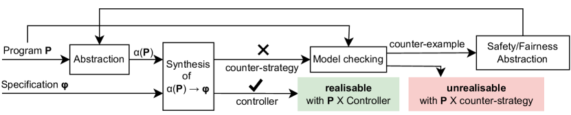
Figure 1. Workflow of our approach.

In this paper, we push the limitations of current automated approaches and manage to solve problems on which existing approaches do not terminate. Our insight is that the currently used abstractions in the community are not rich enough, as they focus on safety abstractions of programs and variables. However there are practical and interesting problems where the abstractions also need to capture fairness properties of the program. We show how to identify when these fairness refinements are needed, how to compute them, and how they can be incorporated in a workflow with standard safety abstractions, resulting in an approach that pushes the limits of what current methodologies can solve. We are not aware of a comparable approach.

We focus on LTL reactive synthesis, with specifications as LTL formulas over propositional variables controlled by the environment or by the controller. We also expect a deterministic reactive program that acts as the arena on which the environment and controller play, i.e. the program reacts to the actions of both. The LTL specifications can also talk about the state of the program. Concretely, one can see the reactive program as a set of atomic methods, some only callable by the environment and others only by the controller, where moreover the controller has the ability to react immediately to any call of the environment. This reactive program can manipulate variables with an infinite domain, thus acting as an infinite-state arena. We model these programs as a form of symbolic automata. Theoretically our approach is limited to theories amenable to interpolation, in practice and in examples we focus on programs integer programs with addition and subtraction.

Fig. 1 illustrates the workflow of our approach, also implemented in a prototype. This describes a largely standard CEGAR loop for infinite-state synthesis — we abstract the program as an LTL formula, give control of it to the environment, and use counterexamples that witness the spuriousness of abstract counterstrategies to add relevant predicates to the abstraction. Our main contribution here is that we use counterexamples, when of a certain form, to identify relevant fairness properties of the program. Namely, if the counterexample exposes a failed attempt at a loop in the counter strategy, then we apply termination checking to identify a ranking function for the corresponding program behaviour. Given this ranking function, we can augment the abstraction with a strong fairness assumption on the behaviour of the program, eliminating an infinite-family of similar counterstrategies. We describe this workflow informally in more detail in Sec. 3.

Contributions. Our main contribution is the inclusion of fairness aspects in an automated CEGAR-based practical synthesis approach to the control problem of infinite-state reactive programs with respect to LTL specifications. We provide a proof-of-concept implementation, with a DSL for writing reactive programs, and use it to evaluate the viability of this approach through experiments. Our approach has the following advantages over comparable work:

1. Unbounded Reasoning: Unlike existing automated work we are able to reason over unboundedly many steps, since we consider fairness properties of the program.

2. Generality: We go beyond safety and reachability, and consider full LTL properties, for which we are able to terminate on problems that comparable solutions do not terminate on.

3. Automation: Our approach is fully automated, and requires no strategy templates, unlike the only previous comparable approach that incorporated some fairness aspects. Templates encode some of the required memory needed to solve the problem, which requires substantial investment and knowledge about the program. That said, in our prototype we allow users, when they have a rough solution in mind, to suggest state predicates and fairness properties, which may accelerate the process.

4. Applications: We show how our approach has several applications, including automatically extending/repairing programs given new specifications and functionality. Furthermore, we equip this prototype with a DSL for writing reactive programs, avoiding the need to manually write programs in form of transition systems.

In Sec. 2 we give a brief background in LTL and synthesis. In Sec. 3 we informally describe our approach, showing how we solve a challenging example from literature, and describe briefly our prototype’s DSL for reactive programs. We then start the formal presentation. In Sec. 4 we introduce our formalism for reactive programs, continuing in Sec. 5 by stating the synthesis problem we tackle and characterising the properties of different parts of our algorithm. In Sec. 6 we define predicate abstraction for our programs, and in Sec. 7 we specify how to check whether an abstract counter strategy is spurious, and when to apply safety or fairness refinement. In Sec. 8 we describe briefly our prototype, its applications on several case studies, including program extension and repair examples, and present some experiments. We conclude with some future work in Sec. 9. In Sec. References we give proofs for the claims made, and present some more case studies.

Related Work. We now describe related work in this area in detail. In literature we find several semi-automated or automated approaches that fit or can be made to fit our stated goal of controlling infinite-state programs. These approaches are almost all based on some abstraction-refinement approach, given the infinite-state nature of the problem.

On the semi-automated side, a notable approach is that of DBLP:conf/popl/BeyeneCPR14. They describe an efficient method to encode general LTL and $\omega$-regular games using Constrained Horn Clauses and solve them using constraint solving. In this framework, one can encode programs as transition systems and define LTL goals over them (as Büchi automata). However, the user must also provide a template of the strategy/controller, while writing a specification can already be demanding on the user. In practice this means the user has to have extensive knowledge about the problem in question, and a good idea of the way to solve it. If we see the controller as Mealy machines, the user has to give a Mealy Machine with some inputs and outputs left undefined, and then the problem becomes “can we fill in these undefined inputs and outputs such that the Mealy machine is a controller for our specification?”. Thus, failing to find a solution does not equate to the problem being unrealisable, since an actual controller may need a different structure, states, or actions. Similar to our approach, they require finding ranking functions to witness the progress of the entire strategy towards achieving its goals (for non-safety games). Contrarily, we “learn” local progress arguments for parts of the program, to exclude spurious counterstrategies. The authors report very fast runtime, once one has found a suitable controller template. Our automated approach instead learns incrementally the structure and memory the controller needs, a somewhat harder problem.

On the automated side we find several approaches. DBLP:conf/icalp/HenzingerJM03 suggest a framework on how to use a CEGAR approach to solve infinite-state $\omega$-regular games. Through model checking they identify counterexamples to abstract counterstrategies, which are in turn used to refine abstract states into multiple more concrete states. Our approach follows a similar flow, except we do not just refine abstract states but also add fairness constraints, while we start with a concrete program.

Other promising approaches are limited in the games they consider, unlike our approach that is applicable to full LTL. 10.1145/3158149 give a complete algorithm for satisfiability games and another sound algorithm for reachability games. 10.1007/978-3-319-89963-3_10 consider safety games and apply their algorithm to Lustre programs, forcing safety invariants to be maintained after each time step. 8894254 use machine learning to synthesise safety controllers which is guaranteed to converge if they can find a decision tree abstraction of the winning region.

Another line of work is based on synthesising reactive programs from different variations of Temporal Stream Logic (TSL) specifications. TSL is essentially LTL with atoms as predicates and updates in some background theory (e.g., linear arithmetic), and can be used to encode our programs. 10.1007/978-3-030-25540-4_35 cast this problem into standard LTL synthesis, allowing the controller to control updates and the environment to control the predicates. They use reactive synthesis to search for implementations. If an abstract counter strategy is spurious, environment assumptions to prevent it are added. These assumptions talk about the effects of an update in the next state. A limitation of this approach is that the underlying background is left uninterpreted at the reactive synthesis level, such that the controller must work for every possible interpretation. 10.1145/3519939.3523429 tackle this problem by using syntax-guided synthesis to synthesise implementations (respecting some grammar) for data-transformation tasks in the specification that respect the underlying interpretation. These are then added to the specification, leaving reactive synthesis to deal with the control aspects of the problem. MaderbacherBloem22 take a similar approach, where they exclude spurious counterstrategies with new state assumptions, predicates and transition constraints, keeping track also of invariant relations between predicates.

These approaches have a limited focus. On one side we have those that are only able to deal with safety or reachability specifications. The others attempt more expressive specifications but do not consider rich enough abstractions of the program or background theory — namely they do not consider fairness aspects. MaderbacherBloem22 illustrate concisely the negative effects of this limitation with a simple problem that their, and other related, approaches cannot solve: given an integer variable $x$ with an arbitrary initial value chosen by the environment, where the controller has the power to increment or decrement while the environment has no power over it, synthesise a controller that makes the value of $x$ negative. A simple obvious solution exists, a controller that repeatedly decrements $x$. These approaches attempt enumerating all the possible positive values of $x$, never terminating. Instead, for our algorithm this example is very simple, by learning the fact that decrementing repeatedly a positive value eventually results in a negative value we can avoid an infinite number of state predicates, as we show in Sec. 3.

Synthesis in an infinite-state context is undecidable in general. However, 10.1007/3-540-44685-0_36 characterise games under which an abstraction-refinement approach can succeed and terminate, under safety refinements (i.e. refining of abstract games states). Another approach by cesarcav casts the problem into a decidable problem, but giving controllers that are not directly applicable to the original problem. They consider synthesis of specifications over a variation of LTL with atoms as predicates over possibly non-Boolean variables, with no notion of actions/updates on the variables. Instead of using abstraction-refinement, they immediately create a sound and complete equi-realisable abstraction of a specification from this extension of LTL into standard boolean LTL. Predicates over non-boolean are abstracted into variables, and constraints are added that relate the predicate variables according to the underlying theory (e.g., $x\geq 0$ cannot be true while $x=-1$ is true). The controller or counter strategy one gets here is simply an interaction of over valuations of their respective predicates. It is not obvious how to create an implementation from this template, while single steps here may require multiple steps in an actual implementation (given a limited set of environment and controller actions). This seems to imply that the original specification may not hold over a final implementation.

The supervisory control problem is also related to ours, although the focus is usually on limited properties (e.g., state avoidance) and finite-state systems, although we find some work in the infinite setting. DBLP:journals/deds/KalyonGMM12 give an undecidable algorithm to control for infinite-state safety specifications of symbolic transition systems. They further use abstract interpretation to overapproximate the state space to give an effective algorithm, that may return a spurious counterstrategy. Our work considers more general properties and focusses on an infinite trace setting. 10.1145/3501710.3519535 present an abstraction-refinement synthesis loop when the program is a continuous dynamical system, a substantially different setting from ours. However, interestingly, they use bounded synthesis to ensure small controllers and attempt the synthesis of abstract controllers and counterstrategies in parallel. To our knowledge, fairness is not considered.

2. Background: LTL and Mealy and Moore Machines

Linear Temporal Logic LTL$(\mathbb{AP})$ is the language over a set of propositions $\mathbb{AP}$, defined as follows, where $p\in\mathbb{AP}$:

$$\phi \mathrel{\overset{\makebox[0.0pt]{\mbox{\tiny def}}}{=}}\textbf{tt}\mid\textbf{ff}\mid p\mid\neg p\mid\phi\wedge\phi\mid\phi\vee\phi\mid X\phi\mid\phi U\phi\mid G\phi\mid F\phi\mid\phi W\phi$$

See (DBLP:reference/mc/PitermanP18) for the standard semantics of LTL, omitted here. For $w\in(2^{\mathbb{AP}})^{\omega}$, we write $w\models\phi$ or $w\in L(\phi)$, when $w$ satisfies $\phi$.

A Moore machine is $C=\langle S,s_{0},\Sigma_{in},\Sigma_{out},\rightarrow,out\rangle$, where $S$ is the set of states, $s_{0}$ the initial state, $\Sigma_{in}$ the set of input events, $\Sigma_{out}$ the set of output events, $\rightarrow:S\times\Sigma_{in}\hookrightarrow S$ the complete deterministic transition function, and $out:S\rightarrow\Sigma_{out}$ the labelling of each state with an output event. For $(s,I,s^{\prime})\in\rightarrow$, where $out(s)=O$ we write $s\xrightarrow{I/O}s^{\prime}$, i.e. we add $out(s)$ to all outgoing transitions of $s$.

A Mealy machine is $C=\langle S,s_{0},\Sigma_{in},\Sigma_{out},\rightarrow\rangle$, where $S$, $s_{0}$, $\Sigma_{in}$, and $\Sigma_{out}$ are as before and $\rightarrow:S\times\Sigma_{in}\hookrightarrow\Sigma_{out}\times S$ the complete deterministic transition function. For $(s,I,O,s^{\prime})\in\rightarrow$ we write $s\xrightarrow{I/O}s^{\prime}$.

Notice that by definition for every state $s\in S$ and every $I\in\Sigma_{in}$ there is $O\in\Sigma_{out}$ and $s^{\prime}$ such that $s\xrightarrow{I/O}s^{\prime}$.

Unless mentioned explicitly, both Mealy and Moore machines can have an infinite number of states. A run of a machine $C$ is $r=s_{0},s_{1},\ldots$ such that for every $i\geq 0$ we have $s_{i}\xrightarrow{I_{i}/O_{i}}s_{i+1}$ for some $I_{i}$ and $O_{i}$. Run $r$ produces the word $w=\sigma_{0},\sigma_{1},\ldots$, where $\sigma_{i}=I_{i}\cup O_{i}$. We say that a machine $C$ produces the word $w$ if there exists a run $r$ producing $w$.

The LTL reactive synthesis problem calls for finding a Mealy machine that satisfies a given specification.

Definition 2.1 (LTL Synthesis).

A specification $\phi$ over $\mathbb{E}\cup\mathbb{C}$ is said to be realisable if and only if there is a Mealy machine $C$, with input $2^{\mathbb{E}}$ and output $2^{\mathbb{C}}$, such that for every $w\in L(C)$ we have $w\models\phi$. We call $C$ a controller for $\phi$.

A specification $\phi$ is said to be unrealisable if there is a Moore machine $CS$, with input $2^{\mathbb{C}}$ and output $2^{\mathbb{E}}$, such that for every $w\in L(CS)$ we have that $w\models\neg\phi$. We call $CS$ a counter strategy for $\phi$.

Note that the duality between the existence of a strategy and counter strategy follows from the determinacy of turn-based two-player $\omega$-regular games (10.2307/1971035). We know that finite-state machines suffice for synthesis from LTL specifications (DBLP:conf/popl/PnueliR89).

3. Informal Overview

In this section, we informally introduce our approach, aided by examples. We first give an intuition of the way we cast the synthesis problem, and then look at examples with reachability and repeated reachability of problems with unbounded variables that are a challenge for existing work.

Figure 2. Program in which the environment sets a value of unbounded integer variable $x$, and the controller is then fully in control of incrementing or decrementing $x$ ($inc$ and $dec$ are controller variables).

From a game perspective, in our approach the game arena on which the environment and controller play is a reactive program, expressed as a symbolic automaton. Fig. 2 illustrates an example of such an automaton. This representation is akin to the control-flow graph of a program, and we use it as the basis for synthesis. We describe a more practical DSL for writing reactive programs and how a corresponding symbolic automaton can be created from it in Sec. 3.2.

This automaton manipulates its variables, $\mathbb{V}$, here $x$ and goal. The program state can be exposed through Boolean program output variables, $\mathbb{M}$, here goal. Note that $\mathbb{M}$ is always a subset of $\mathbb{V}$. Program outputs are the only program variables we allow mentioned in the user-given LTL specification. Here, we define an output as a predicate that is evaluated on the program state after each transition, but in general we allow it to be a Boolean variable that is updated on each transition. As in standard synthesis, other Boolean variables appearing in the specification can be controlled by the environment, $\mathbb{E}$, here start and inc_env, or by the controller, $\mathbb{C}$, here inc_con.

Transitions are partitioned into two kinds: those controlled by the environment (solid ones) and those by the controller (dashed ones). Transitions are labelled by guarded actions, $\textit{guard}\mapsto action$, where the guard can range over the program variables and the environment (controller) variables. As in standard synthesis, in every time-step the environment acts, and in the same time step the controller responds. In our context the reactive program reacts to both in the same time-step. In Fig. 3 we illustrate how the described interaction manifests in a run.

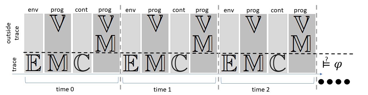
Figure 3. The order of variable updates over time, in a trace.

First the program reacts to the environment (take a solid transition depending on $\mathbb{E}$), and updates its variables $\mathbb{V}$ (including the externally visible $\mathbb{M}$) and then reacts to the controller (taking a dashed transition depending on $\mathbb{C}$) and updates $\mathbb{V}$ accordingly. Note program output variables also change in reaction to the controller, but this is only perceived in the next time step (if not overwritten).

In the example, in the first time-step the environment has three choices. Either it sets start to true and the program moves to $q1$, or depending on the value of inc_env it can either increment or decrement $x$. Essentially, at $q_{0}$ the environment controls the value of $x$. In $q1$ the controller is instead fully in control of $x$, and has the choice to decrement or increment it accordingly. With regard to program output, after each environment transition, goal is set to false if $x$ is non-negative, and $true$ otherwise throughout the execution.

Finally, we assume the program is deterministic since we are interested in manipulating implementations — any non-determinism is resolved by adding appropriate environment variables.

Given this overview of the formal context, we consider how to derive a controller that drives programs to satisfy a given specification. We solve this problem through a CEGAR loop (as in Fig. 1). All definitions and the approach are made formal in the sections following this one.

3.1. Solving Problems with Unboundedly Many Steps

Looking at Fig. 2, as introduced earlier, consider the reachability goal $\phi\mathrel{\overset{\makebox[0.0pt]{\mbox{\tiny def}}}{=}}(F\ \textit{start})\implies F(\textit{start}\wedge F\ \textbf{goal})$, i.e. if the environment settles on a value for $x$ then the controller has the goal to force $x$ to a negative value. The repetition of start on the left-hand side of the implication ensures that the obligation on goal holds after start happens. This example casts in our framework the challenge example from MaderbacherBloem22, which illustrates the limitations of existing infinite-state synthesis approaches. We describe how our fairness abstraction solves this.

We start by using standard methods from predicate abstraction to create a finite-state abstraction of the reactive program. The initial abstraction is based on the program output variables (goal, i.e. $x<0$), and the automaton states. This is illustrated in Fig. 4. Abstractions have only Boolean variables, exposed in the abstract states, which are pairs of a control state of the program and assignments to Boolean variables. Note how this abstraction is non-deterministic unlike the concrete program. The two outgoing transitions from the initial state illustrate how the value of $x$ can be chosen to be non-negative or negative, leading to states with, respectively, goal to be false or true. There is also non-determinism at $q1$, since, incrementing a negative value may possibly lead to a non-negative one (e.g., if $x=-2$ then incrementing it leaves it negative, but not if $x=-1$).

Figure 4. Predicate abstraction of Fig. 2.

We now attempt to synthesise a controller based on this abstract program. We create a synthesis problem where the environment controls, in addition to its own variables, variables for encoding the states ($q_{0}$ and $q_{1}$) and output (predicate) variables (goal) of the program. We write an LTL formula characterising all the computations that can arise in the abstract program and add it as an assumption to the LTL specification. That is, if $\alpha({\mathcal{P}})$ is the formula capturing the abstraction, the new specification is $\alpha({\mathcal{P}})\rightarrow\phi$. The LTL formula $\alpha({\mathcal{P}})$ needs to impose the correct time steps: environment variables, solid arcs, and control variables are set (in this order) every time step. Thus, the LTL formula makes visible the state that is the target of a solid arc and between every two time steps variables change according to the sequential combination of a dashed and a solid arc.

Figure 5. Abstract counterstrategy to Fig. 4.

Figure 6. Abstract controller for Fig. 4 and $\phi$.

Since the environment is in control of the abstract program’s transitions, reactive synthesis gives us an abstract counterstrategy here. We show this in Fig. 6, in a similar Mealy machine expanded format as our programs and abstractions. Strictly speaking, we expect counterstrategies that are Moore machines, but they can be re-written as Mealy machines. In this, the environment chooses to go immediately to $q1$ with goal set to false, and remain there whatever the controller does. To determine whether this is a real counterstrategy, we compose it with the concrete program (Fig. 2) and use model checking to search for states where there is a disagreement on the control state or on the values of predicates, which we term compatibility checking. This gives us a counterexample wherein if in the first step the environment does start, and thus $x$ is set to 0, then the controller can do decrement (through $\neg\textit{inc\_con}$) and the program thus sets goal to true, while the environment desired goal to be false. At this point, purely safety/state-based approaches, like existing approaches, can use this counterexample to discover the predicate $x=0$ and add it to the abstraction. Re-attempting the same safety approach would end up non-terminating: in the next step the predicate $x=1$ will be discovered, and so on, i.e. the algorithm will attempt to enumerate $\mathbb{N}$. On the other hand, we avoid this by immediately and automatically identify a fairness property of the program.

Our main insight is that the counterexample exposes a spurious cycle in the abstract counterstrategy in Fig. 6. Note how the environment attempts to remain in a cycle, by first visiting $s_{1}$ and then attempts to return to it after the controller forces a decrement of $x$. However, at this point the transition setting goal to false mismatches with the concrete program state, for the discovered counterexample. Moreover, all possible counterexamples have this mismatch, up to some arbitrary bound. We use a ranking function as a witness for the termination of the controller’s behaviour to exclude the corresponding infinite family of spurious abstract counterstrategies.

We first collect the program actions corresponding to the attempted counterstrategy cycle, here simply $x:=x-1$. We further look at the failed environment transition, i.e. $q_{1}\wedge\neg\textbf{goal}$. We ignore state variables, and consider the predicate definition of output variables, thus we are left with $\neg x<0$, which is equivalent to $x\geq 0$.

We create a while-program corresponding to this cycle, with the while condition being $x\geq 0$ and $x:=x-1$ as the body of the loop. In general, we also consider restrictions on the value of $x$ before the loop is entered by looking at the value of predicates or of variables, however this is not required here. Our algorithm feeds this while-program to a termination checker, and extracts a ranking function as a witness for termination. The ranking function we get here is equivalent to the function $x$. We also get an associated invariant $x\geq 0$, given $x$ is an integer function, i.e. $x$ is only a ranking function in the space where it never decrements beyond 0.

We proceed by encoding the proof of termination of this behaviour in the abstraction. We add three new transition predicates. We identify decrements of $x$ with $x^{dec}\mathrel{\overset{\makebox[0.0pt]{\mbox{\tiny def}}}{=}}x>x^{\prime}$, increments of $x$ with $x^{inc}\mathrel{\overset{\makebox[0.0pt]{\mbox{\tiny def}}}{=}}x<x^{\prime}$, and violation of the invariant after a transition with $x^{\neg inv}\mathrel{\overset{\makebox[0.0pt]{\mbox{\tiny def}}}{=}}\neg(x^{\prime}\geq 0)$. After adding these, the new abstraction corresponds to the old one with abstract target states of transitions decrementing $x$ augmented with the transition predicate $x^{dec}$ and those states after incrementing $x$ by $x^{inc}$, and those violating the invariant by $x^{\neg inv}$. Then our algorithm automatically constructs a strong fairness assumption true in the program, stating that “if $x$ decreases infinitely often then $x$ must increase infinitely often or violate the invariant”, i.e. $(GF\ x^{dec})\implies(GF\ (x^{inc}\vee x^{\neg inv}))$.

With this assumption our approach is able to quickly terminate: having performed only one refinement, the next abstract synthesis step produces a controller, shown in Fig. 6. This controller simply does $\neg\textit{inc\_con}$ at each state, then eventually the environment must start (otherwise $\phi$ is satisfied) and that decrements and no increments eventually force the environment to make goal true (due to the invariant), ensuring $\phi$ is satisfied. For presentation, we ignore transitions where the environment breaks the assumptions (e.g., not following correctly the program control-flow).

This example illustrates our main contribution, how we go beyond existing automated approaches to terminate and solve problems that require reasoning over an unbounded number of steps by bypassing an infinite number of safety refinements in one step.

Next, we exemplify how to incorporate the new fairness refinement with state/safety refinement. We also take the opportunity to introduce our DSL.

3.2. Solving Repeated Reachability with Unbounded Variables

⬇

1int cnt := 0;

2bool done_requests := false;

3

4method extern request(){

5 assume(!done_requests);

6 cnt++;

7}

8

9method extern service(){

10 assume(!done_requests);

11 done_requests := true;

12}

⬇

13method intern grant(){

14 assert(done_requests);

15 // ... code to handle job ...

16 cnt--;

17}

18

19method intern finish(){

20 assert(done_requests);

21 assert(cnt == 0);

22 done_requests := false;

23}

Figure 7. Reactive program with functionality to receive and handle jobs.

Consider the reactive program in Fig. 7. This is written in our DSL for reactive programs, which our tool accepts as input. One can define Boolean, integer, or natural-number variables (bounded or unbounded; with enum types as syntactic sugar for bounded integers). Boolean variables may be marked as output variables. Furthermore, we allow defining different methods performing some non-looping actions on the variable state. Methods can be marked as extern or intern, denoting respectively that the methods may be called by the environment or by the desired controller. intern methods then are the tools a prospective controller can use to enforce a certain specification on the program. Methods can also have Boolean parameters. Assumptions govern when external methods can be called, while the controller must ensure that no assertions are violated.

Such programs can be translated into a symbolic automaton, with unparameterised methods corresponding to propositional variables and parameterised methods have in addition a variable for each parameter. Currently we use a Boolean variable done_requests to denote different states of a program; we currently compile our DSL into an automaton with a single control state, and rely on assumptions and assertions to encode control flow. In addition, to model the behaviour of assume and assert, we add two sink states that capture respective violations. The automatically constructed automaton is shown in Fig. 8, with the sink states omitted.

Figure 8. Automaton corresponding to program in Fig. 7, with every omitted environment or controller transitions respectively going to $env\_err$ or $sys\_err$ states.

This program expects a continuous sequence of requests. It counts the length of the sequence using the variable cnt and at some point decides that it is time to serve (service) these requests. Then, the program expects the controller to reply with a sequence of grants ending with a finish. The program forces the sequence of grants to be of the same length as the sequence of requests by asserting that finish is called at the right moment. Once a grant sequence finishes successfully the program is ready for a new request sequence. The additional LTL specification is $\phi=G(\textit{service}\implies F\ \textit{finish})$. If the controller does not grant adequately, the program will either violate an assert or end up with a negative value of cnt and never be able to finish. Note that neither the counter nor the length of the sequence are bounded. When translating the program to an automaton, the LTL specification is changed automatically to $\phi^{+}\mathrel{\overset{\makebox[0.0pt]{\mbox{\tiny def}}}{=}}G(\neg\mbox{{env\_err}})\rightarrow G(\neg\mbox{{sys\_err}})\wedge\phi$, where env_err is the state resulting from calling an external method that violates an assume and sys_err is the state resulting from violating an assert. We do not explicitly add Boolean output variables for env_err and sys_err. Later on, we add Boolean variables for all states of the automaton as part of our synthesis algorithm. With this symbolic automaton and the specification in place, we show how our approach can determine the realisability of the specification and identify a realising controller.

As before, we start with a finite-state abstraction that exposes only the structure of the program. The first abstraction is shown in Fig. 9. Unlike the program, this abstraction is non-deterministic: in state $q_{2}$ $\textit{finish}\wedge\neg\textit{grant}$ can lead either to $q_{1}$ or to $env\_err$.

We now attempt to synthesise a controller based on this abstract program. We create a synthesis problem where the environment controls, in addition to its own variables (service and request), variables for encoding the states ($q_{1},q_{2}$, $sys\_err$, and $env\_err$). We write $\alpha_{1}({\mathcal{P}})$ for the LTL formula corresponding to this abstract program.

In our case, the problem $\alpha_{1}({\mathcal{P}})\rightarrow\phi^{+}$ is unrealisable. We extract a counter strategy manifesting the unrealisability (not depicted). This counter strategy immediately sets service to true leaving $q_{1}$ and regardless of the controller’s value of grant, it proceeds to set request and service to false forever (i.e., it reaches state $q_{2}$ and stays there forever).

Through model checking we identify a counterexample where the counter strategy attempts to stay in $q_{2}$, but where the concrete program does not. By using interpolation techniques on this trace we identify the predicate $cnt=0$ as an interpolant, and add it to the abstraction, avoiding this spurious counter strategy. We fast forward to the point when the predicate $cnt=1$ is also identified as an interpolant and use the two predicates to refine the abstraction. The result is the abstract program in Fig. 10. As before, we omit states $sys\_err$ and $env\_err$ and the respective transitions leading to them. As customary, we write only the Boolean variables set to true, e.g., $\{cnt=1\}$ represents the valuation where $cnt=0$ is false, while $cnt=1$ is true.

Figure 9. The initial abstraction of program in Fig. 8 (as before, missing transitions go to their respective error states, and here also the dangling transition).

Figure 10. A later finite-state predicate abstraction of the program in Fig. 8 (here we also assume mutual exclusivity between the method call variables, to keep the figure digestable, and use $idle\_E\mathrel{\overset{\makebox[0.0pt]{\mbox{\tiny def}}}{=}}\neg(\textit{request}\vee\textit{service})$ and $idle\_C\mathrel{\overset{\makebox[0.0pt]{\mbox{\tiny def}}}{=}}\neg(\textit{grant}\vee\textit{finish})$).

The abstract program is still nondeterministic. For example, two dashed arcs from state $(q_{2},\{\})$ are labelled by $\neg\textit{finish}$ and grant, both satisfied by $\textit{grant}\wedge\neg\textit{finish}$. As before, we add variables $q_{1}$, $q_{2}$, $sys\_err$ and $env\_err$ as well as the predicates $cnt=0$ and $cnt=1$ as new variables controlled by the environment. Let $\alpha_{2}({\mathcal{P}})$ denote the LTL formula capturing all computations of this refined program over these variables. The new specification $\alpha_{2}({\mathcal{P}})\rightarrow\phi^{+}$ is still unrealisable. The counter strategy, this time, issues two requests before attempting to stay in state $(q_{2},\{\})$ forever. This counter strategy is also infeasible. However, the infeasibility manifests in a loop.

Rather than attempting to find more state predicates, which inevitably leads to an infinite sequence of refinements, we check whether the loop is terminating. A model checker confirms that indeed it is and our approach divines the ranking function $cnt$ and the invariant $cnt\geq 0$. As before, we add three predicates $cnt^{dec}$, $cnt^{inc}$, and $cnt^{\neg inv}$ to the target states of transitions that, respectively, decrease the counter, increase it, and violate the invariant. Let $\alpha_{l}=GF(cnt^{dec})\implies GF\ (cnt^{inc}\vee\neg cnt^{\neg inv})$. Then, $\alpha_{3}({\mathcal{P}})$ is the LTL formula describing the allowed changes to $q_{1}$, $q_{2}$, $sys\_err$, and $env\_err$ and the variables $cnt=0$, $cnt=1$, $cnt<0$, $cnt^{dec}$, $cnt^{inc}$, and $cnt^{\neg inv}$, conjuncted with $\alpha_{l}$. Finally, we check realisability of $\alpha_{3}({\mathcal{P}})\rightarrow\phi^{+}$, resulting in a positive answer and a controller. We construct a final controller by supplying the synthesised controller with information on how the program resolves the nondeterminism of the abstract program.

4. Symbolic Automata as a formalism for Reactive Programs

We formalise the programs presented in Section 3 as symbolic automata. A reactive program interacts with both the environment and the controller: namely, it can read their respective variables and update its own Boolean variables that the other two can read. To account for this interaction with two different entities, we use a variant of existing symbolic automata formalisms (DBLP:conf/fmics/ColomboPS08; atva21) and specialise the notation and functionality for our needs. Here, we dedicate space to introduce these variations in detail. Our automata have a finite number of (control) states and manipulate variables that can range over infinite domains. Transitions are guarded by conditions on non-program variables, and values of internal program variables. Furthermore, transitions can update the internal variables by means of assignments. We distinguish between transitions that interact with the environment and the controller.

While the program manipulates variables with (potentially) infinite domains, the interaction between the environment, controller, and program occurs using a set of Boolean variables, which also serve as the propositions in the LTL specification we synthesise for. Thus, we write $\mathbb{E}$, $\mathbb{C}$, and $\mathbb{M}$, respectively for non-intersecting environment, controller, and program variables. For example, in Fig. 2, we have $\mathbb{E}=\{inc\_env,start\}$, $\mathbb{C}=\{inc\_con\}$, and $\mathbb{M}=\{goal\}$. In Fig. 8, we have $\mathbb{E}=\{request,service\}$, $\mathbb{C}=\{\textit{grant},\textit{finish}\}$, and $\mathbb{M}=\{\}$. We use $E$, $C$, and $M$ respectively for subsets of $\mathbb{E}$, $\mathbb{C}$, and $\mathbb{M}$.

Given an infinite trace $w$ over $2^{\mathbb{AP}}$, we denote by ${w}{\Downarrow}_{S}$ the point-wise projection of $w$ on $S\subseteq\mathbb{AP}$: ${w}{\Downarrow}_{S}(i)=w(i)\cap S$.

Definition 4.1 (Symbolic Automata).

A symbolic automaton, or automaton for short, is a tuple ${\mathcal{P}}=\langle\mathbb{V},\Theta,Q,\theta_{0},q_{0},\rightarrow,\dashrightarrow\rangle$, where

1. $\mathbb{V}$ is a set of typed variables, with $\mathbb{M}\subseteq\mathbb{V}$; we call $\mathbb{V}\setminus\mathbb{M}$ internal variables and $\mathbb{M}$ external variables. Variable domains can be infinite (e.g., $\mathbb{N}$).

2. $\Theta$ is the set of possible valuations of $\mathbb{V}$,

3. $Q$ is a finite set of states,

4. $\theta_{0}\in\Theta$ is the initial variable valuation,

5. $q_{0}\in Q$ is the initial state, and

6. $\rightarrow:Q\times\mathcal{B}(\mathbb{E}\cup\mathbb{V})\hookrightarrow\mathcal{A}(\mathbb{V})\times Q$ and $\dashrightarrow:Q\times\mathcal{B}(\mathbb{C}\cup\mathbb{V})\hookrightarrow\mathcal{A}(\mathbb{V})\times Q$ are symbolically guarded partial transition functions that respectively react to the environment (reading $\mathbb{E}$) and the controller (reading $\mathbb{C}$).

For a set of variables $V$, we write $\mathcal{B}(V)$ for the set of possible Boolean combinations of predicates over $V$ with type-consistent values; we write $\mathcal{A}(V)$ for the set of transformations over $V$, i.e., functions from $V$ to formulas over $V$ with type-consistent values. We write $\theta_{V}\models g$, where $g\in\mathcal{B}(V)$, to denote that the valuation $\theta_{V}$ models the Boolean formula $g$. For $a\in\mathcal{A}(V)$ we write $a(\theta_{V})$ for the valuation $\theta_{V}$ updated according to the assignment $a$, if it is defined for it.

For $(q,g,a,q^{\prime})\in\rightarrow$ we write $q\xrightarrow{g\mapsto a}q^{\prime}$ (and similarly for $\dashrightarrow$).

In Fig. 8, we have $Q=\{q_{1},q_{2},err_{\mathbb{C}},err_{\mathbb{E}}\}$, $\mathbb{V}=\{cnt:\mathbb{N}\}$, and $\theta_{0}=\{cnt\mapsto 0\}$. Note how $\neg request$ and $cnt=1$ are in $\mathcal{B}(\mathbb{V}\cup\mathbb{E})$, and $a_{1}\mathrel{\overset{\makebox[0.0pt]{\mbox{\tiny def}}}{=}}cnt:=cnt-1$ and $a_{2}\mathrel{\overset{\makebox[0.0pt]{\mbox{\tiny def}}}{=}}cnt:=cnt+1$ are in $\mathcal{A}(\mathbb{V})$. The transition function $\rightarrow$ consists of all the solid arcs, and $\dashrightarrow$ of the dashed arcs.

As explained, our synthesis process incorporates three agents (environment, program, and controller). In the usual setting of controller synthesis, in every time step, the environment sets the values of its variables and the controller reacts by setting the values of its variables. Here, we have the program reacting to the environment and to the controller. However, rather than memorising the controller variables and allowing the program to react to them only in the next time step, the program reacts to the controller variables immediately (without registering changes in the outputs ($\mathbb{M}$) of the resulting trace), cf. Fig. 3. The presence of the two transition functions does not add expressivity, however it allows for automata with size $|\rightarrow|+|\dashrightarrow|$ rather than $|\rightarrow|\times|\dashrightarrow|$.

Throughout the rest of the paper we restrict attention to symbolic automata that are complete, deterministic, and preserve well-typedness of the variables, and refer to them also as programs.

Definition 4.2 (Program).

A program is an automaton where (1-completeness) every state has an outgoing environment (controller) transition for every possible valuation; (2-determinism) every two environment (controller) transitions from the same state have mutually exclusive guards $g_{1}$ and $g_{2}$; and (3-well-typedness) every transition’s action is well-defined for every model of its guard.

Program semantics is given by two transition relations over configurations:

Definition 4.3 (Semantics).

The semantics of a symbolic automaton is given over configurations from $Q\times\Theta_{\mathbb{V}}$, with $(q_{0},\theta_{0})$ as the initial configuration.

The semantics of an environment transition is given with a function $\delta_{\mathbb{E}}:(Q\times\Theta_{\mathbb{V}})\times\Theta_{\mathbb{E}}\rightarrow(Q\times\Theta_{\mathbb{V}})$, updating the configuration according to the transition that matches the current configuration and the environment valuation:

$$\delta_{\mathbb{E}}((q,\theta_{\mathbb{V}}),\theta_{\mathbb{E}})\mathrel{\overset{\makebox[0.0pt]{\mbox{\tiny def}}}{=}}(q^{\prime},a(\theta_{\mathbb{V}}))\ \text{ where }\ \exists g,a\cdot q\xrightarrow{g\mapsto a}q^{\prime}\textit{ and }\theta_{\mathbb{V}}\cup\theta_{\mathbb{E}}\models g$$

The semantics of controller transitions are defined similarly:

$$\delta_{\mathbb{C}}((q,\theta_{\mathbb{V}}),\theta_{\mathbb{C}})\mathrel{\overset{\makebox[0.0pt]{\mbox{\tiny def}}}{=}}(q^{\prime},a(\theta_{\mathbb{V}}))\ \text{ where }\ \exists g,a\cdot q\ext@arrow 0359 \relbar {g\mapsto a}q^{\prime}\textit{ and }\theta_{\mathbb{V}}\cup\theta_{\mathbb{C}}\models g$$ →

In one step the program takes both an environment and a controller transition:

$$\delta((q,\theta_{\mathbb{V}}),\theta)\mathrel{\overset{\makebox[0.0pt]{\mbox{\tiny def}}}{=}}\delta_{\mathbb{C}}(\delta_{\mathbb{E}}((q,\theta_{\mathbb{V}}),\theta|_{\mathbb{E}}),\theta|_{\mathbb{C}})$$

Let $\delta^{*}$ be the reflexive transitive closure of $\delta$ operating on $(2^{\mathbb{E}\cup\mathbb{C}})^{*}$.

For example, the program in Fig. 8 has configurations in $Q\times\mathbb{N}$, e.g., $(q_{1},0)$ is the initial configuration, where $0$ is the value of $cnt$. We have $\delta_{\mathbb{E}}((q_{1},0),\{request\})=(q_{1},1)$ and $\delta_{\mathbb{E}}((q_{1},0),\{service\})=(q_{2},0)$. Similarly, we have $\delta_{\mathbb{C}}((q_{2},1),\{grant\})=(q_{2},0)$ and $\delta_{\mathbb{C}}((q_{2},0),\{\})=(q_{1},0)$. We write variables that are true and omit those that are false, e.g., $\{\}$ is the assignment of all variables to false. The joint transition $\delta((q_{1},0),\{request,grant\})=(err_{\mathbb{C}},1)$ and $\delta((q_{1},2),\{request,grant\})=(err_{\mathbb{E}},2)$.

Definition 4.4 (Run).

For a program ${\mathcal{P}}$ and a word $w\in 2^{\mathbb{E}\cup\mathbb{C}}$, let the run $run_{{\mathcal{P}}}((q,\theta_{\mathbb{V}}),w)$ be $(q,\theta_{\mathbb{V}}),(q_{0}^{\prime},\theta_{0}^{\prime}),\ldots$ such that $(q^{\prime}_{i},\theta^{\prime}_{i})=\delta_{\mathbb{E}}((q_{i},\theta_{i}),{w_{i}}{\Downarrow}_{\mathbb{E}})$ and $(q_{i+1},\theta_{i+1})=\delta_{\mathbb{C}}((q^{\prime}_{i},\theta^{\prime}_{i}),{w_{i}}{\Downarrow}_{\mathbb{C}})$. Let $run^{\mathbb{C}}$ be the projection of $run$ on odd (primed) positions.

In all notations, we remove the subscript ${\mathcal{P}}$ and remove $(q,\theta_{\mathbb{V}})$ when $q=q_{0}$ and $\theta_{\mathbb{V}}=\theta_{0}$. For example, for the program in Fig. 8 and $w_{1}=\{\textit{request}\}^{\omega}$ we have $run(w_{1})=(q_{0},0),(q_{0},1)$, $(q_{0},1),(q_{0},2),(q_{0},2),\ldots$, and for $w_{2}=\{\textit{service},\textit{finish}\}^{\omega}$ we have $run(w_{2})=run(w_{2},(q_{1},0))=(q_{1},0),(q_{2},0),(q_{1},0),(q_{2},0),\ldots$. We have $run^{\mathbb{C}}(w_{2})=(q_{2},0),(q_{2},0,),\ldots$.

Definition 4.5 (Program Language).

We write $w\models{\mathcal{P}}$ if $w$ is the point-wise union of a word $w_{\mathbb{E},\mathbb{C}}\in(2^{\mathbb{E}\cup\mathbb{C}})^{\omega}$, and $w_{\mathbb{M}}$ for the output trace of ${\mathcal{P}}$, s.t. $w_{\mathbb{M}}={run^{\mathbb{C}}(w_{\mathbb{E}\cup\mathbb{C}})}{\Downarrow}_{\mathbb{M}}$.

In Fig. 8, $\{\textit{service},\textit{finish}\}^{\omega}\models{\mathcal{P}}$, i.e., service and finish are always signalled and neither sys_err nor env_err are ever signalled. Also, $\{\textit{request}\},\{\textit{service}\},\{\textit{finish}\},\{sys\_err\}^{\omega}\models{\mathcal{P}}$. Although the program reaches $err_{\mathbb{C}}$ in the time step finish is signalled it only can output $sys\_err$ in the next.

5. Infinite-state Synthesis with Abstraction-Refinement

We are now ready to define the synthesis problem that we handle in this paper, and to explain at a high-level the procedures it uses in order to solve the synthesis problem. We first define synthesis with safety abstractions of the program in our framework (similar to what existing approaches do), and then describe how to integrate into that knowledge of fairness properties of the program relevant to synthesis, the main insight of this paper.

Note that this synthesis problem is undecidable and our algorithm may still not terminate even if all procedure calls within it terminate (some of the procedures are undecidable and potentially non-terminating in their own right). However, our extension with fairness abstractions adds value by allowing our procedure to terminate in cases where safety abstraction is known not to terminate.

5.1. The Synthesis Problem

In our setting the controller operates against both an environment (controlling $\mathbb{E}$) and a program ${\mathcal{P}}$ (controlling $\mathbb{M}$), a generalization of the traditional setting. That is, as part of the global environment some inputs are uncontrollable, while others are generated by a white-box program (Defn. 4.2).

Definition 5.1 (Synthesis Against a Program).

A specification ${\mathcal{P}}\rightarrow\phi$, over $\mathbb{E}\cup\mathbb{C}\cup\mathbb{M}$, is said to be realisable if there is a Mealy machine $C$, with input $\mathbb{E}\cup\mathbb{M}$ and output $\mathbb{C}$, such that for every $w\in L(C)$ if $w\models{\mathcal{P}}$ then $w\models\phi$. We call $C$ a controller for ${\mathcal{P}}\rightarrow\phi$. Otherwise it is unrealisable.

From determinacy of turn-based two-player games with Borel objectives (10.2307/1971035) it follows that if a problem is unrealisable, then there is a counter strategy.

Definition 5.2 (Counter strategy).

A counter strategy to the realisability of a specification ${\mathcal{P}}\rightarrow\phi$ is a Moore machine $CS$, with input $\mathbb{C}$ and output $\mathbb{E}\cup\mathbb{M}$, such that for every $w\in L(CS)$ we have that $w\models{\mathcal{P}}$ and $w\not\models\phi$.

If we have an appropriate controller $C$ for $\phi$, then we are finished. This essentially means that $C$ does not require knowledge of ${\mathcal{P}}$ to ensure $\phi$. However, such knowledge may be needed in the general case, requiring both safety and fairness facts about the program. Next, we describe how to discover these incrementally, starting with safety and then moving to fairness.

5.2. Synthesis Algorithm with Safety Abstraction

1 Function synthesise(${\mathcal{P}}$, $\phi$):

2       $\mathbb{S}\leftarrow Q_{{\mathcal{P}}}\cup\mathbb{M}_{{\mathcal{P}}}$; while true do

3             $\alpha_{s}({\mathcal{P}})\leftarrow\mathtt{abstract\_LTL\_formula}({\mathcal{P}},\mathbb{S})$

4             if $\mathtt{is\_realisable}(\alpha_{s}({\mathcal{P}})\rightarrow\phi,\mathbb{E}\cup Q\cup\mathbb{S},\mathbb{C})$ then

5                   return $(\textit{true},\texttt{strategy}(\alpha_{s}({\mathcal{P}})\rightarrow\phi,\mathbb{E}\cup Q\cup\mathbb{S},\mathbb{C}))$

6                  

7            $\textit{MM}\leftarrow\texttt{counter\_strategy}(\alpha_{s}({\mathcal{P}})\rightarrow\phi,\mathbb{E}\cup Q\cup\mathbb{S},\mathbb{C})$

8             if $\mathtt{compatible}({\mathcal{P}},\textit{MM})$ then  return $(\textit{false},\textit{MM})$

             $ce\leftarrow\texttt{compatibility\_counterexample}({\mathcal{P}},\textit{MM})$

              // Here MM is      

             $\mathbb{S}\leftarrow\mathbb{S}\cup\texttt{safety\_refinement}({\mathcal{P}},\textit{MM},ce)$

              // a spurious counter strategy      

9            

10      

Algorithm 1 CEGAR-based Synthesis Algorithm with Safety Refinements

The first synthesis algorithm is formally presented as Algorithm 1. The algorithm starts with a program ${\mathcal{P}}$ and an LTL formula $\phi$. It maintains a set of state predicates $\mathbb{S}$ (always including $\mathbb{M}$). Based on $\mathbb{S}$, it produces an LTL formula $\alpha_{s}({\mathcal{P}})$ whose set of traces over-approximates that of the program. We then check if it is possible to realise a controller for $\alpha_{s}({\mathcal{P}})\rightarrow\phi$. That is, check for the existence of a controller such that interacting with programs satisfying $\alpha_{s}({\mathcal{P}})$ (in particular, ${\mathcal{P}}$) satisfies the specification $\phi$. A strategy that realises $\alpha_{s}({\mathcal{P}})\rightarrow\phi$, can be converted to a strategy that realises ${\mathcal{P}}\rightarrow\phi$. If $\alpha_{s}({\mathcal{P}})\rightarrow\phi$ is unrealisable, we get a Moore machine MM that is a counter strategy to its realisability, and which we check for compatibility with ${\mathcal{P}}$. If the counter strategy is compatible with the program, it corresponds to a real counter strategy to ${\mathcal{P}}\rightarrow\phi$. Otherwise, there exists a finite counter example $ce$. Based on $ce$ we refine the predicates and re-attempt.

We give some details about the procedures/subroutines that we use. We assume familiarity with standard LTL synthesis and give no further details about related implementations. For other procedures, we state their properties as assumptions, which help us explain the algorithm. The procedures and their assumptions are made more general when we explain the fairness extension. We then formalise and concretise the procedures in the full algorithm in Sec. 6 and Sec. 7, where we also discharge the stronger assumptions.

Starting with the standard tools of LTL synthesis, we use the following subroutines. First, $\mathtt{is\_realizable}(\phi,\mathbb{I},\mathbb{O})$ checks whether the LTL formula $\phi$ over atomic propositions $\mathbb{AP}=\mathbb{I}\cup\mathbb{O}$ is realisable, with $\mathbb{I}$ to be controlled by the environment and $\mathbb{O}$ controlled by the controller. For a realisable formula $\phi$, we have $\mathtt{strategy}(\phi,\mathbb{I},\mathbb{O})$ as a routine that returns a strategy in the form of a Mealy machine. Dually, for an unrealisable formula $\phi$, $\mathtt{counter\_strategy}(\phi,\mathbb{I},\mathbb{O})$ returns a counter strategy in the form of a Moore machine.

The algorithm $\mathtt{abstract\_LTL\_formula}({\mathcal{P}},\mathbb{S})$ takes a program ${\mathcal{P}}$, and a set of state predicates over $\mathbb{V}$ (the variables of ${\mathcal{P}}$). That is, state predicates characterise sets of assignments to $\mathbb{V}$. The algorithm outputs an LTL formula $\alpha_{s}({\mathcal{P}})$ over $\mathbb{AP}=\mathbb{E}\cup\mathbb{C}\cup\mathbb{M}\cup Q\cup\mathbb{S}$ that over approximates the traces of ${\mathcal{P}}$. Particularly, we treat the set of states $Q$ of ${\mathcal{P}}$ as propositions.

More formally, we define the following abstractions $\alpha$. We do not explicitly write the set $\mathbb{S}$, although all the abstractions are parameterised by it. For any variable valuation $\theta$, let $\alpha(\theta)=\{s\in\nolinebreak\mathbb{S}\mid\theta\models s\}$: that is, the set of state predicates in $\mathbb{S}$ that are satisfied by the valuation $\theta$. As $\theta$ is a valuation, it follows that for every $s\in\mathbb{S}\setminus\alpha(\theta)$ we have $\theta\models\neg s$. Consider a word $w\in(2^{\mathbb{E}\cup\mathbb{C}})^{\omega}$ and the run $r=run_{\mathcal{P}}(w)=(q_{0},\theta_{0}),(q^{\prime}_{0},\theta^{\prime}_{0}),\ldots$. Let $\alpha(r)=A^{\prime}_{0},A^{\prime}_{1},\ldots$, where $A^{\prime}_{i}=\{q^{\prime}_{i}\}\cup w_{i}\cup\alpha(\theta^{\prime}_{i})$. That is, $\alpha(r)$ looks on the configurations of the form $(q^{\prime}_{i},\theta^{\prime}_{i})$ of ${\mathcal{P}}$ from which a $\mathbb{C}$ transition is about to be taken. It collects the state $q^{\prime}_{i}$ of the configuration, the propositions from $\mathbb{E}$ and $\mathbb{C}$ from the input $w_{i}$, and the predicates from $\mathbb{S}$ that are satisfied by $\theta^{\prime}_{i}$. We note that $\alpha(r)$ is a word over the set of propositions $\mathbb{AP}$ above.

Finally, we can state that $\alpha_{s}({\mathcal{P}})$ is an abstraction of the program ${\mathcal{P}}$:

Assumption 1-$\mathcal{A}$ 0 (Abstract Safety).

Given a set of predicates $\mathbb{S}$ and the formula $\alpha_{s}({\mathcal{P}})=\mathtt{abstract\_LTL\_formula}({\mathcal{P}},\mathbb{S})$ then for every word $w\in(2^{\mathbb{E}\cup\mathbb{C}})^{\omega}$ we have $\alpha(run(w))\models\alpha_{s}({\mathcal{P}})$.

Assumption 1-$\mathcal{A}$ implies that $\alpha_{s}({\mathcal{P}})$ abstracts ${\mathcal{P}}$.

The procedure $\mathtt{compatible}({\mathcal{P}},\textit{MM})$ takes a program ${\mathcal{P}}$ and a Moore machine MM that is a counter strategy for $\alpha_{s}({\mathcal{P}})\rightarrow\phi$. It returns true when MM is a counter strategy for ${\mathcal{P}}\rightarrow\phi$. It returns false when there exists a finite counter example $ce$ such that $ce$ is a prefix of a word produced by MM but there exists no run $r$ of ${\mathcal{P}}$ such that $\alpha(r)$ has the prefix $ce$. Notice that MM defines a language over $\mathbb{AP}$ and thus the word produced by MM includes also the sequence of states of ${\mathcal{P}}$ (as well as $\mathbb{E}$ and $\mathbb{C}$). Furthermore, the procedure $\mathtt{compatibility\_counterexample}({\mathcal{P}},\textit{MM})$ returns such a counter example $ce$.

Assumption 3 (Compatibility).

Procedure $\mathtt{compatible}({\mathcal{P}},\textit{MM})$ satisfies that:

• If it returns true then MM is a counter strategy to ${\mathcal{P}}\rightarrow\phi$.

• If it returns false then $\mathtt{compatibility\_counterexample}({\mathcal{P}},\textit{MM})$ returns a counter example $w$ such that for some $w^{\prime}$ we have $w\cdot w^{\prime}$ is produced by MM but there does not exist $w^{\prime\prime}$ and run $r$ of ${\mathcal{P}}$ such that $w\cdot w^{\prime\prime}=\alpha(r)$.

The procedure $\mathtt{safety\_refinement}({\mathcal{P}},\textit{MM},ce)$ takes the program, the counter strategy, and a counter example. It returns a set of state predicates $S$ corresponding to the unfeasibility of $ce$ in ${\mathcal{P}}$.

Assumption 4 (Safety Refinement).

Let $S$ be the set of predicates returned by the procedure $\mathtt{safety\_refinement}({\mathcal{P}},\textit{MM},ce)$. Then, MM is not a counter strategy for $\alpha_{s}({\mathcal{P}})\rightarrow\phi$, where $\alpha_{s}({\mathcal{P}})$ is computed with respect to $\mathbb{S}\cup S$.

Based on these assumptions, we can state the soundness of Algorithm 1.

If Algorithm 1 terminates, then the following holds:

• If the algorithm returns $(\textit{true},C)$, where $C$ is a Mealy machine, then ${\mathcal{P}}\rightarrow\phi$ is realisable and $C$ realises it.

• If the algorithm returns $(\textit{false},\textit{MM})$, where MM is a Moore machine, then ${\mathcal{P}}\rightarrow\phi$ is unrealisable and MM is a counter strategy.

Proof.

The case of realisability follows from the soundness of abstractions in Assumptions 1 and 2. Indeed, by these assumptions $\alpha_{sf}({\mathcal{P}})$ is sound. That is, for every $w\in(2^{\mathbb{E}\cup\mathbb{C}})^{\omega}$ we have $\alpha(run(w))\models\alpha_{sf}({\mathcal{P}})$.

Consider a strategy $C$ realising $\alpha_{sf}({\mathcal{P}})\rightarrow\phi$. We use $C$ as follows. Given an input $E\subseteq\mathbb{E}$, use ${\mathcal{P}}$ to resolve the state $q\in Q$ and the predicates in $\mathbb{S}\cup\mathbb{T}$. Use this combination in order to give an input $I$ in $2^{\mathbb{E}\cup Q\cup\mathbb{S}\cup\mathbb{T}}$ to $C$. As $C$ is a Mealy machine, its transition reading $I$ is labeled by some $O\subseteq\mathbb{C}$. This is the output of the strategy. We then feed $O$ to the program. The same is repeated for the next input. Consider an infinite trace over $\mathbb{E}\cup\mathbb{M}\cup\mathbb{C}$ produced this way and let $r$ by the induced run of ${\mathcal{P}}$. By the assumptions $\alpha(r)\models\alpha_{sf}({\mathcal{P}})$. As the controller realises $\alpha_{sf}({\mathcal{P}})\rightarrow\pi$ it must be the case that the trace satisfies $\pi$.

The case of unrealisability follows directly from the first part of Assumption 3. ∎

5.3. Extending Safety Abstractions with Fairness

1 Function synthesise(${\mathcal{P}}$, $\phi$):

2       $\mathbb{S}\leftarrow Q_{{\mathcal{P}}}\cup\mathbb{M}_{{\mathcal{P}}}$; $\color[rgb]{0,0,1}{\mathbb{T}\leftarrow\emptyset}$

3       while true do

4             $\alpha_{s}({\mathcal{P}})\leftarrow\mathtt{abstract\_LTL\_formula}({\mathcal{P}},\mathbb{S}\color[rgb]{0,0,1}{,\mathbb{T}})$

5             $\color[rgb]{0,0,1}{\alpha_{f}({\mathcal{P}})\leftarrow\mathtt{strong\_fairness}(\mathbb{T})}$

6             $\color[rgb]{0,0,1}{\alpha_{sf}({\mathcal{P}})=\alpha_{s}({\mathcal{P}})\wedge\alpha_{f}({\mathcal{P}})}$

7             if $\mathtt{is\_realisable}({\color[rgb]{0,0,1}{\alpha_{sf}({\mathcal{P}})}}\rightarrow\phi,\mathbb{E}\cup Q\cup\mathbb{S}{\color[rgb]{0,0,1}{\cup\mathbb{T}}},\mathbb{C})$ then

8                   return $(\textit{true},\texttt{strategy}({\color[rgb]{0,0,1}{\alpha_{sf}({\mathcal{P}})}}\rightarrow\phi,\mathbb{E}\cup Q\cup\mathbb{S}{\color[rgb]{0,0,1}{\cup\mathbb{T}}},\mathbb{C}))$

9                  

10            $\textit{MM}\leftarrow\texttt{counter\_strategy}(\alpha_{sf}({\mathcal{P}})\rightarrow\phi,\mathbb{E}\cup Q\cup\mathbb{S}{\color[rgb]{0,0,1}{\cup\mathbb{T}}},\mathbb{C})$

11             if $\mathtt{compatible}({\mathcal{P}},\textit{MM})$ then  return $(\textit{false},\textit{MM})$

             $ce\leftarrow\texttt{compatibility\_counterexample}({\mathcal{P}},\textit{MM})$

              // Here MM is      

             $\mathbb{S}\leftarrow\mathbb{S}\cup\texttt{safety\_refinement}({\mathcal{P}},\textit{MM},ce)$

              // a spurious      

             $\color[rgb]{0,0,1}{\mathbb{T}\leftarrow\mathbb{T}\cup\texttt{fairness\_refinement}({\mathcal{P}},\textit{MM},ce)}$

              // counter strategy

12            

13      

Algorithm 2 CEGAR-based Synthesis Algorithm with Safety and Fairness Refinements

The algorithm described in the previous section is in the same family as pre-existing algorithms (e.g., (DBLP:conf/icalp/HenzingerJM03; MaderbacherBloem22)). Hence it is liable to require an infinite number of refinements (and predicates) when attempting to solve some simple problems, including those in Sec. 3. Here we augment the previous algorithm with a notion of program fairness, further restricting the environment in its interpretation of the program semantics.

Our full synthesis algorithm is formally presented as Algorithm 2. The previous algorithm is extended to also keep track of a set of transition predicates, producing an LTL formula $\alpha_{sf}({\mathcal{P}})$ as an abstraction of the program.

For this, the algorithm $\mathtt{abstract\_LTL\_formula}$ is extended to be also parametrised on $\mathbb{T}$, a set of transition predicates over $\mathbb{V}$ and $\mathbb{V}^{\prime}$. That is, transition predicates characterise relations over $\mathbb{V}$. The algorithm outputs an LTL formula $\alpha_{s}({\mathcal{P}})$ over $\mathbb{AP}=\mathbb{E}\cup\mathbb{C}\cup\mathbb{M}\cup Q\cup\mathbb{S}\cup\mathbb{T}$ that over approximates the traces of ${\mathcal{P}}$.

We extend the abstraction $\alpha$ parametrised by $\mathbb{T}$ as $\alpha(\theta,\theta^{\prime})=\{t\in\mathbb{T}~{}|~{}(\theta,\theta^{\prime})\models t\}$. That is, the set of transition predicates in $\mathbb{T}$ that are satisfied by the pair of valuations $(\theta,\theta^{\prime})$. As $\theta$ and $\theta^{\prime}$ are valuations it follows that for every $t\in\mathbb{T}\setminus\alpha(\theta,\theta)$ we have $(\theta,\theta^{\prime})\models\neg t$. Consider a word $w\in(2^{\mathbb{E}\cup\mathbb{C}})^{\omega}$ and the run $r=run_{\mathcal{P}}(w)=(q_{0},\theta_{0}),(q^{\prime}_{0},\theta^{\prime}_{0}),\ldots$. Let $\alpha(r)=A^{\prime}_{0},A^{\prime}_{1},\ldots$, where $A^{\prime}_{0}=\{q^{\prime}_{0}\}\cup w_{0}\cup\alpha(\theta^{\prime}_{0})\cup\alpha(\theta_{0},\theta^{\prime}_{0})$ and $A^{\prime}_{i+1}=\{q^{\prime}_{i+1}\}\cup w_{i+1}\cup\alpha(\theta^{\prime}_{i+1})\cup\alpha(\theta^{\prime}_{i},\theta_{i+1})\cup\alpha(\theta_{i+1},\theta^{\prime}_{i+1})$. Now $\alpha$ also collects both the transition predicates that were true over the one before last transition from $\theta^{\prime}_{i-1}$ to $\theta_{i}$ and the last transition from $\theta_{i}$ to $\theta^{\prime}_{i}$.

We generalise Assumption 1-$\mathcal{A}$ to take also transition predicates into account. As before, the assumption implies that $\alpha_{s}({\mathcal{P}})$ abstracts ${\mathcal{P}}$.

Assumption 1 (Abstract Safety).

Given a set of predicates $\mathbb{S}$ and $\mathbb{T}$ and the formula $\alpha_{s}({\mathcal{P}})=\mathtt{abstract\_LTL\_formula}({\mathcal{P}},\mathbb{S},\mathbb{T})$ then for every word $w\in(2^{\mathbb{E}\cup\mathbb{C}})^{\omega}$ we have $\alpha(run(w))\models\alpha_{s}({\mathcal{P}})$.

The algorithm $\mathtt{strong\_fairness}(\mathbb{T})$ takes the set of transition predicates $\mathbb{T}$, using these to create an LTL formula over propositions $\mathbb{T}$. We assume that $\mathbb{T}$ is composed of triples of predicates $\langle t^{dec},t^{inc},t^{\neg inv}\rangle$ of the form $t^{dec}\mathrel{\overset{\makebox[0.0pt]{\mbox{\tiny def}}}{=}}f>f^{\prime}$, $t^{inc}\mathrel{\overset{\makebox[0.0pt]{\mbox{\tiny def}}}{=}}f<f^{\prime}$, and $t^{\neg inv}\mathrel{\overset{\makebox[0.0pt]{\mbox{\tiny def}}}{=}}\neg\textit{invar}^{\prime}_{f}$, where $f$ is a function over $\mathbb{V}$ that is well-founded over the invariant $\textit{invar}_{f}$. Then, $\alpha_{f}({\mathcal{P}})=\mathtt{strong\_fairness}(\mathbb{T})$ is $\bigwedge_{{\langle{t^{dec},t^{inc},t^{\neg inv}}\rangle}\in\mathbb{T}}(GF(t^{dec})\rightarrow GF(t^{inc}\vee t^{\neg inv}))$. This is an abstraction of ${\mathcal{P}}$:

Assumption 2 (Abstract Fairness).

Given a set of predicates $\mathbb{T}$ and the formula $\alpha_{f}({\mathcal{P}})=\mathtt{strong\_fairness}(\mathbb{T})$ then for every word $w\in(2^{\mathbb{E}\cup\mathbb{C}})^{\omega}$ we have $\alpha(run(w))\models\alpha_{f}({\mathcal{P}})$.

Assumptions 1 and 2 imply that $\alpha_{sf}({\mathcal{P}})=\alpha_{s}({\mathcal{P}})\wedge\alpha_{f}({\mathcal{P}})$ abstracts ${\mathcal{P}}$.

We modify procedure $\mathtt{compatible}({\mathcal{P}},\textit{MM})$ to check a counter strategy for $\alpha_{sf}({\mathcal{P}})\rightarrow\phi$. That is, $\mathtt{compatible}$ is extended to consider also the set of predicates $\mathbb{T}$. It still maintains the same property, Assumption 3, which we do not restate. We also do not restate Assumption 4, which holds for the more general formula $\alpha_{s}({\mathcal{P}})$ that depends also on $\mathbb{T}$.

The procedure $\mathtt{fairness\_refinement}({\mathcal{P}},\textit{MM},ce)$ takes the program, the predicates, and a counter example. If the counter example corresponds to a loop in the program for which termination can be proven, the procedure returns transition predicates of the form $f>f^{\prime}$, $f<f^{\prime}$, and $\neg\textit{invar}^{\prime}_{f}$, where $f$ is a ranking function in the state space satisfying the invariant $\textit{invar}_{f}$.

Assumption 5 (Fairness Refinement).

Let $T$ be the set of predicates returned by the procedure $\mathtt{fairness\_refinement}({\mathcal{P}},\textit{MM},ce)$. Then, MM is not a counter strategy for $\alpha_{f}({\mathcal{P}})\rightarrow\phi$, where $\alpha_{f}({\mathcal{P}})$ is computed with respect to $\mathbb{T}\cup T$.

Based on these assumptions, we can state the soundness of Algorithm 2.

If Algorithm 2 terminates, then the following holds:

• If the algorithm returns $(\textit{true},C)$, where $C$ is a Mealy machine, then ${\mathcal{P}}\rightarrow\phi$ is realisable and $C$ realises it.

• If the algorithm returns $(\textit{false},\textit{MM})$, where MM is a Moore machine, then ${\mathcal{P}}\rightarrow\phi$ is unrealisable and MM is a counter strategy.

Proof.

The case of realisability follows from the soundness of abstractions in Assumptions 1 and 2. Indeed, by these assumptions $\alpha_{sf}({\mathcal{P}})$ is sound. That is, for every $w\in(2^{\mathbb{E}\cup\mathbb{C}})^{\omega}$ we have $\alpha(run(w))\models\alpha_{sf}({\mathcal{P}})$.

Consider a strategy $C$ realising $\alpha_{sf}({\mathcal{P}})\rightarrow\phi$. We use $C$ as follows. Given an input $E\subseteq\mathbb{E}$, use ${\mathcal{P}}$ to resolve the state $q\in Q$ and the predicates in $\mathbb{S}\cup\mathbb{T}$. Use this combination in order to give an input $I$ in $2^{\mathbb{E}\cup Q\cup\mathbb{S}\cup\mathbb{T}}$ to $C$. As $C$ is a Mealy machine, its transition reading $I$ is labeled by some $O\subseteq\mathbb{C}$. This is the output of the strategy. We then feed $O$ to the program. The same is repeated for the next input. Consider an infinite trace over $\mathbb{E}\cup\mathbb{M}\cup\mathbb{C}$ produced this way and let $r$ by the induced run of ${\mathcal{P}}$. By the assumptions $\alpha(r)\models\alpha_{sf}({\mathcal{P}})$. As the controller realises $\alpha_{sf}({\mathcal{P}})\rightarrow\pi$ it must be the case that the trace satisfies $\pi$.

The case of unrealisability follows directly from the first part of Assumption 3. ∎

In the next sections, we formalise the treatment of all the procedures explained above and discharge assumptions 1–5. Notice that we discharge the more general assumptions and the simpler ones follow as well. Find all proofs in the appendix.

6. Predicate Abstraction

In this section we define the abstract formula $\alpha_{sf}({\mathcal{P}})$, but first we formalise the application of predicate abstraction to programs. Abstract programs are also used for compatibility and counter examples to compatibility in Section 7.

We work with a set of state predicates $\mathbb{S}$ and a set of transition predicates $\mathbb{T}$. Recall the following: (1) $s\in\mathbb{S}$corresponds to a set of valuations $\{\theta\models s\}$; (2) $t\in\mathbb{T}$corresponds to a relation $\{(\theta,\theta^{\prime})\models t\}$; and (3) the set $\mathbb{T}$ is composed of triples ${\langle{t^{dec},t^{inc},t^{\neg inv}}\rangle}$ corresponding to a function with a well-founded range. For example, in our running example, $cnt=0$ is a state predicate and $cnt^{dec}\mathrel{\overset{\makebox[0.0pt]{\mbox{\tiny def}}}{=}}cnt>cnt^{\prime}$ is the transition predicate whose counterpart is $cnt^{inc}\mathrel{\overset{\makebox[0.0pt]{\mbox{\tiny def}}}{=}}cnt<cnt^{\prime}$, with the invariant violation predicate $cnt^{\neg inv}\mathrel{\overset{\makebox[0.0pt]{\mbox{\tiny def}}}{=}}cnt^{\prime}<0$.

Definition 6.1 (Atom).

Given a set of predicates $\mathbb{P}$ an atom is $A\subseteq\mathbb{P}$. Given an atom $A\subseteq\mathbb{P}$, let $\mathrm{conj}(A)=\bigwedge_{p\in A}p\wedge\bigwedge_{p\in\mathbb{P}\setminus A}\neg p$.

We restrict attention to atoms $A$ such that $\mathrm{conj}(A\cap\mathbb{S})$ is satisfiable. Let $at(\mathbb{P})$ be the set of atoms over $\mathbb{P}$. In the running example, given the set of state predicates $\{cnt=0,cnt=1\}$ and transition predicates $\{cnt^{inc},cnt^{dec},cnt^{\neg inv}\}$, we have $\{cnt=0,cnt=1\}$ is an unsatisfiable atom, $\{\}$ and $\{cnt=1\}$ are satisfiable atoms, and $\mathrm{conj}(\{cnt=1\})\mathrel{\overset{\makebox[0.0pt]{\mbox{\tiny def}}}{=}}(cnt=1)\wedge(cnt\neq 0)\wedge\neg cnt^{dec}\wedge\neg cnt^{inc}\wedge\neg cnt^{\neg inv}$. Notice that $A=\{cnt=1,cnt^{dec},cnt^{inc},cnt^{\neg inv}\}$ is an atom as $\mathrm{conj}(A\cap\mathbb{S})$ is satisfiable. Indeed, we may need to store both $t^{inc}$ and $t^{dec}$ in the same atom, as we see in a few paragraphs.

Definition 6.2 (Predicate Abstraction of Program).

Given a program ${\mathcal{P}}$, the abstract program $\alpha({\mathcal{P}})$ is an automaton with no internal variables, with states $\hat{Q}=Q\times 2^{\mathbb{S}\cup\mathbb{T}}$ and initial state $\hat{q_{0}}\mathrel{\overset{\makebox[0.0pt]{\mbox{\tiny def}}}{=}}(q_{0},\alpha(\theta))$. Recall that given a valuation $\theta$ we have $\alpha(\theta)$ as $\{s\in\mathbb{S}~{}|~{}\theta\models s\}$ and $\alpha(\theta,\theta^{\prime})$ as $\{t\in\mathbb{T}~{}|~{}(\theta,\theta^{\prime})\models t\}$:

1. $(q,P)\xrightarrow{\ E\ }(q^{\prime},P^{\prime})\mathrel{\overset{\makebox[0.0pt]{\mbox{\tiny def}}}{=}}\exists\theta,\theta^{\prime}.P\cap\mathbb{S}=\alpha(\theta),P^{\prime}=\alpha(\theta^{\prime})\cup\alpha(\theta,\theta^{\prime}),\delta_{\mathbb{E}}((q,\theta),E)=(q^{\prime},\theta^{\prime})$; and

2. $(q,P)\ext@arrow 0359$ $\relbar$ →${\ C\ }(q^{\prime},P^{\prime})\mathrel{\overset{\makebox[0.0pt]{\mbox{\tiny def}}}{=}}\exists\theta,\theta^{\prime}.P\cap\mathbb{S}=\alpha(\theta),P^{\prime}=\alpha(\theta^{\prime})\cup\alpha(\theta,\theta^{\prime}),\delta_{\mathbb{C}}((q,\theta),C)=(q^{\prime},\theta^{\prime})$.

Fig. 9 is the predicate abstraction of Fig. 8 with $\mathbb{S}=\{\}$ and Fig. 10 is the predicate abstraction of Fig. 8 with $\mathbb{S}=\{cnt=0,cnt=1\}$. For example, in Fig. 10 the dashed transition from $(q_{2},\{\})$ to $(q_{2},\{cnt=1\})$ labelled $\mathit{grant}$ results from the self loop labelled $\mathit{grant}\wedge\neg\mathit{finish}\mapsto cnt{\raisebox{1.07639pt}{\tiny\bf\textminus\textminus}}$ on $q_{2}$ in Fig. 8. Indeed, for the valuation $\theta$ setting $cnt$ to $2$ and $\theta^{\prime}$ setting $cnt$ to $1$ we have $\{cnt=1,cnt=0\}\cap\alpha(\theta)=\emptyset$, $\{cnt=1\}=\alpha(\theta^{\prime})$, and $\delta_{\mathbb{C}}(q_{2},\theta),\{grant\})=(q_{2},\theta^{\prime})$.

For $w\in(2^{\mathbb{E}\cup\mathbb{C}})^{\omega}$ let $run_{P}(w)=(q_{0},\theta_{0}),(q^{\prime}_{0},\theta^{\prime}_{0}),\ldots$. The run $(q_{0},P_{0}),(q^{\prime}_{0},P^{\prime}_{0}),\ldots$, where $P_{0}=\alpha(\theta_{0})$, $P^{\prime}_{i}=\alpha(\theta^{\prime}_{i})\cup\alpha(\theta_{i},\theta^{\prime}_{i})$, and $P_{i+1}=\alpha(\theta_{i+1})\cup\alpha(\theta^{\prime}_{i},\theta_{i+1})$, is a run of $\alpha({\mathcal{P}})$ induced by $w$.

Proof.

By definition, we have $\hat{q_{0}}=(q_{0},\alpha(\theta_{0}))$. Furthermore, consider a transition $(q^{\prime}_{i},\theta^{\prime}_{i})=\delta_{\mathbb{E}}((q_{i},\theta_{i}),w_{i}\cap\mathbb{E})$. By definition, $(q_{i},P_{i})\xrightarrow{w_{i}\cap\mathbb{E}}(q^{\prime}_{i},P^{\prime}_{i})$. Similarly, if $(q_{i+1},\theta_{i+1})=\delta_{\mathbb{C}}((q^{\prime}_{i},\theta^{\prime}_{i}),w_{i}\cap\mathbb{C})$ then $(q^{\prime}_{i},P^{\prime}_{i})\ext@arrow 0359$ $\relbar$ →${w_{i}\cap\mathbb{C}}(q_{i+1},P_{i+1})$. ∎

Given a predicate abstraction of a program we construct a corresponding LTL abstraction. This causes further loss of detail. First, we restrict attention to the intermediate states in the run of ${\mathcal{P}}$ in which the transitions reading the controller input are applied. Second, transition predicates collect what happened to the formulas they follow over the last two changes of variables. Recall that transition predicates capture decrease and increase from states that satisfy the invariant of formulas, and maintenance of an invariant. We store a decrease if there is an decrease in one of the steps, and similarly for increase and violation of the invariant. It follows that the LTL formula can allow the transition predicates, in particular increase and decrease, to occur at the same time.

Definition 6.3 (Abstract Characteristic Formula).

The abstract characteristic formula of abstract program ${\alpha({{\mathcal{P}}})}$, written ${\alpha_{{}_{s}}({{\mathcal{P}}})}$, is the conjunction of:

1. initialisation: $\bigvee_{(q_{0},P_{0})\xrightarrow{E}(q,P)}\begin{array}[]{ll}\mathrm{conj}(\{q\}\cup P)\end{array}$; and

2. transition: $G\left(\begin{array}[]{l}\qquad\displaystyle\bigvee q\wedge\mathrm{conj}(P\cup C)\wedge X(\mathrm{conj}(E\cup\{q^{\prime\prime}\}\cup P^{\prime\prime}\cup(P^{\prime}\cap\mathbb{T})))\\[-4.83694pt] {}_{(q,P)\ext@arrow 0359$ \xleaders\hbox{$\relbar$}\hfill\rightarrow${C}(q^{\prime},P^{\prime})\xrightarrow{E}(q^{\prime\prime},P^{\prime\prime})}\end{array}\right)$.

Given program ${\mathcal{P}}$ and sets $\mathbb{S}$ and $\mathbb{T}$, procedure $\mathtt{abstract\_LTL\_formula}({\mathcal{P}},\mathbb{S},\mathbb{T})$ constructs the abstraction as above and gives the abstract characteristic formula of ${\mathcal{P}}$ with respect to $\mathbb{S}$ and $\mathbb{T}$.

For example, the initialisation and transition parts of the abstract program in Fig. 9 include the following. Initially, there are four possible environment choices: (1) following $\mathit{request}\wedge\neg\mathit{service}$ or $\neg\mathit{service}\wedge\neg\mathit{request}$ the program reaches state $q_{1}$, (2) following $\mathit{service}\wedge\neg\mathit{request}$ the program reaches state $q_{2}$, (3) following $\mathit{service}\wedge\mathit{request}$ the program reaches state $env\_err$. Hence, the initialisation is the disjunction of $(q_{1}\wedge\neg q_{2}\wedge\neg sys\_err\wedge\neg env\_err\wedge\neg\mathit{service})$, $(q_{2}\wedge\neg q_{1}\wedge\neg sys\_err\wedge\neg env\_err\wedge\neg\mathit{request}\wedge\mathit{service})$, and $(env\_err\wedge\neq q_{1}\wedge\neg q_{2}\wedge\neg sys\_err\wedge\mathit{request}\wedge\mathit{service})$. Regarding the transition; the disjunct corresponding to the combination of $(q_{2})\ext@arrow 0359$ $\relbar$ →${\{\mathit{grant}\}}(q_{2})$ and $(q_{2})\xrightarrow{\{\}}(q_{2})$ is $(q_{2}\wedge\mathit{grant}\wedge\neg\mathit{finish}\wedge X(\neg\mathit{request}\wedge\neg\mathit{service}\wedge q_{2}\wedge\neg q_{1}\wedge\neg sys\_err\wedge\neg env\_err))$. In the program in Fig. 9 augmented with the predicates $cnt^{dec}$ and $cnt^{inc}$, the transition disjunct corresponding to the combination of $(q_{2})\ext@arrow 0359$ $\relbar$ →${\{\mathit{grant}\}}(q_{2})$ and $(q_{2})\xrightarrow{\{\}}(q_{2})$ is $(q_{2}\wedge\mathit{grant}\wedge\neg\mathit{service}\wedge X(\neg\mathit{request}\wedge\neg\mathit{service}\wedge q_{2}\wedge\neg q_{1}\wedge\neg sys\_err\wedge\neg env\_err\wedge cnt^{dec}\wedge\neg cnt^{inc}))$. In the program in Fig. 8 the situation of both $cnt^{dec}$ and $cnt^{inc}$ never happens in two consecutive transitions. Thus, it is never the case that both $cnt^{dec}$ and $cnt^{inc}$ are true. Since $\mathrm{conj}({q})$ is included in the initialisation and in the next part of every transition disjunct, at every time step exactly one state can be true.

Recall that for a run $r=run_{P}(w)=(q_{0},\theta_{0}),(q^{\prime}_{0},\theta^{\prime}_{0}),\ldots$ we have $\alpha(r)=A^{\prime}_{0},A^{\prime}_{1},\ldots$, where $A^{\prime}_{0}=\{q^{\prime}_{0}\}\cup w_{0}\cup\alpha(\theta^{\prime}_{0})\cup\alpha(\theta_{0},\theta^{\prime}_{0})$ and $A^{\prime}_{i+1}=\{q^{\prime}_{i+1}\}\cup w_{i+1}\cup\alpha(\theta^{\prime}_{i+1})\cup\alpha(\theta^{\prime}_{i},\theta_{i+1})\cup\alpha(\theta_{i+1},\theta^{\prime}_{i+1})$. We discharge Assumption 1:

[Safety Abstraction Correctness] For a word $w\in(2^{\mathbb{E}\cup\mathbb{C}})^{\omega}$ let $run_{\mathcal{P}}(w)=(q_{0},\theta_{0}),(q^{\prime}_{0},\theta^{\prime}_{0}),\ldots$. We have $\alpha(r)\models\alpha_{s}(P)$.

Proof.

By definition $(q^{\prime}_{0},\theta^{\prime}_{0})=\delta_{\mathbb{E}}((q_{0},\theta_{0}),w_{0}\cap\mathbb{E})$ implies that $(q_{0},\alpha(P_{0}))\xrightarrow{w_{0}\cap\mathbb{E}}(q^{\prime}_{0},\alpha(\theta^{\prime}_{0})\cup\alpha(\theta_{0},\theta^{\prime}_{0}))$. Hence, $(q^{\prime}_{0},\alpha(\theta^{\prime}_{0})\cup\alpha(\theta_{0},\theta^{\prime}_{0})))$ satisfies the initialisation part of $\alpha_{s}({\mathcal{P}})$. Furthermore, for every $i>0$ we have $(q_{i},\theta_{i})=\delta_{\mathbb{C}}((q^{\prime}_{i-1},\theta^{\prime}_{i-1}),w_{i-1}\cap\mathbb{C})$ implies $(q^{\prime}_{i-1},\alpha(\theta^{\prime}_{i-1})\cup\alpha(\theta_{i-1},\theta^{\prime}_{i-1}))\ext@arrow 0359$ $\relbar$ →${w_{i-1}\cap\mathbb{C}}(q_{i},\alpha(\theta_{i})\cup\alpha(\theta^{\prime}_{i-1},\theta_{i}))$ and $(q^{\prime}_{i},\theta^{\prime}_{i})=\delta_{\mathbb{E}}((q_{i},\theta_{i}),w_{i}\cap\mathbb{E})$ implies $(q_{i},\alpha(\theta_{i})\cup\alpha(\theta^{\prime}_{i-1},\theta_{i}))\ext@arrow 0359$ $\relbar$ →${w_{i}\cap\mathbb{E}}(q^{\prime}_{i},\alpha(\theta^{\prime}_{i})\cup\alpha(\theta_{i},\theta^{\prime}_{i}))$.

This directly corresponds to the following formula appearing as a disjunct in the transition part of $\alpha_{s}({\mathcal{P}})$.

$$q^{\prime}_{i-1}\wedge conj\left(\alpha(\theta^{\prime}_{i-1}\cup(w_{i-1}\cap\mathbb{C})\right)\wedge$$

$$X\left(conj((w_{i}\cap\mathbb{E})\cup q^{\prime}_{i}\cup\alpha(\theta^{\prime}_{i})\cup\alpha(\theta^{\prime}_{i-1},\theta_{i})\cup\alpha(\theta_{i},\theta^{\prime}_{i}))\right)$$

Hence, $\alpha(r)\models\alpha_{s}({\mathcal{P}})$. ∎

Recall that the transition predicates in $\mathbb{T}$ form triples ${\langle{t^{inc},t^{dec},t^{\neg inv}}\rangle}$, each with a well-founded function $f$. Recall that $\mathtt{strong\_fairness}(\mathbb{T})$ returns $\alpha_{f}({\mathcal{P}})=\bigwedge_{{\langle{t^{dec},t^{inc},t^{\neg inv}}\rangle}\in\mathbb{T}}(GF(t^{dec})\rightarrow GF(t^{inc}\vee t^{\neg inv}))$. We now discharge Assumption 2:

[Fairness Abstraction Correctness] For a word $w\in(2^{\mathbb{E}\cup\mathbb{C}})^{\omega}$ let $run_{P}(w)=(q_{0},\theta_{0}),(q^{\prime}_{0},\theta^{\prime}_{0}),\ldots$. We have $\alpha(r)\models\alpha_{f}({\mathcal{P}})$.

Proof.

Consider a triple of transition predicates ${\langle{t^{dec},t^{inc},t^{\neg inv}}\rangle}$. Let $f$ be the ranking function and $\textit{invar}_{f}$ the corresponding invariant such that $t^{dec}\mathrel{\overset{\makebox[0.0pt]{\mbox{\tiny def}}}{=}}f>f^{\prime}$, $t^{inc}\mathrel{\overset{\makebox[0.0pt]{\mbox{\tiny def}}}{=}}f<f^{\prime}$, and $t^{\neg inv}\mathrel{\overset{\makebox[0.0pt]{\mbox{\tiny def}}}{=}}\neg\textit{invar}^{\prime}_{f}$. Let $run(w)=(q_{0},\theta_{0}),(q^{\prime}_{0},\theta^{\prime}_{0}),(q_{1},\theta_{1}),\ldots$ be a run of ${\mathcal{P}}$. By the range of $f$ being well founded over $\textit{invar}_{f}$, if there are infinitely many locations $i$ such that $f(\theta^{\prime}_{i-1})>f(\theta_{i})$ or $f(\theta_{i})>f(\theta^{\prime}_{i})$, then there must be infinitely many locations $j$ such that $f(\theta^{\prime}_{j-1})<f(\theta_{j})$, $f(\theta_{j})<f(\theta^{\prime}_{j})$, or where $\textit{invar}_{f}$ is violated. However, the case where $f(\theta^{\prime}_{i-1})>f(\theta_{i})$, $f(\theta_{i})>f(\theta^{\prime}_{i})$ is exactly when $t^{dec}$ is in $\alpha(run(w))_{i}$ and the case where $f(\theta^{\prime}_{j-1})<f(\theta_{j})$, $f(\theta_{j})<f(\theta^{\prime}_{j})$, or $\textit{invar}_{f}$ is violated is exactly when $t^{inc}$ or $t^{\neg inv}$ is in $\alpha(run(w))_{j}$. It follows that $\alpha(r)\models\alpha_{f}({\mathcal{P}})$. ∎

As before, let $\alpha_{sf}({\mathcal{P}})=\alpha_{s}({\mathcal{P}})\wedge\alpha_{f}({\mathcal{P}})$. This completes the definition of the predicate abstraction and the abstract LTL formula. We now consider the compatibility of counter strategies and how to refine the abstraction.

7. Compatibility and Refinement

We now turn to the issue of compatibility. We call (counter) strategies derived from $\alpha_{sf}({\mathcal{P}})$ abstract (counter) strategies. From the proof of Theorem 5.3, abstract strategies correspond to real strategies. However, abstract counter strategies can be spurious and expect states or variables to change in ways that are impossible in the program. We define a notion of compatibility capturing when an abstract counter strategy corresponds to a real counter strategy implying unrealisability. We reduce checking compatibility to model checking. When model checking returns a counter example, we show how to extract state or transition predicates that refine the abstraction so that the counter strategy is no longer valid. We also show this infinite-state model checking problem is semi-decidable.

Definition 7.1 (Compatibility).

Consider a program ${\mathcal{P}}$ and a counter strategy MM showing that $\alpha_{sf}({\mathcal{P}})\rightarrow\phi$ is unrealisable. Let $\textit{MM}={\langle{S,s_{0},{\Sigma}_{in},{\Sigma}_{out},\rightarrow,out}\rangle}$, where ${\Sigma}_{in}=2^{\mathbb{C}}$ and ${\Sigma}_{out}=2^{Q\cup\mathbb{E}\cup\mathbb{S}\cup\mathbb{T}}$. We abuse notation and write $out(s)=(q,P)$ for the unique state $q\in Q$ such that $q\in out(s)$ and $P$ for $out(s)\setminus\{q\}$.

Compatibility is defined through two mutually defined simulation relations ${\preceq}_{e}\subseteq(Q\times\Theta)\times(S\times 2^{\mathbb{T}})$ and ${\preceq}_{c}\subseteq(Q\times\Theta)\times S$ that are defined as follows.

For every $(q,\theta)\preceq_{e}(s,T)$, where $out(s)=(q_{s},P_{s})$, it holds that:

1. There is a transition in ${\mathcal{P}}$ from $q$ to $q_{s}$, $q\xrightarrow{g\mapsto a}q_{s}$, s.t. $\theta\cup(P_{s}\cap\mathbb{E})\models g$,

2. The valuation at $q_{s}$ is a model of $P_{s}$’s state predicates: $P_{s}\cap\mathbb{S}=\alpha(a(\theta))$,

3. The transition predicates in $T$, updated with those satisfied over $(\theta,a(\theta))$, are collected in $P_{s}$: $P_{s}\cap\mathbb{T}=T\cup\alpha(\theta,a(\theta))$; and

4. $(q_{s},a(\theta))\preceq_{c}s$.

For every $(q,\theta)\preceq_{c}s$ and for every $C\subseteq\mathbb{C}$, where $out(s)=(q,P)$, $s^{\prime}=\delta(s,C)$, and $out(s^{\prime})=(q_{s^{\prime}},P^{\prime})$, it holds that:

1. There is a transition $q\ext@arrow 0359$ $\relbar$ →${g\mapsto a}q^{\prime}$ s.t. $\theta\cup C\models g$, and $q_{s^{\prime}}$ is reachable in one step from $q^{\prime}$ with an environment transition reading $a(\theta)\cup(P^{\prime}\cap\mathbb{E})$, and

2. $(q^{\prime},a(\theta))\preceq_{e}(s^{\prime},\alpha(\theta,a(\theta)))$.

We say that MM is compatible with $P$ when there are simulation relations such that $(q_{0},\theta_{0})\preceq_{e}(s_{0},\emptyset)$.

The compatibility relation checks whether a counter strategy chooses paths within the abstract program that correspond to runs of the concrete program. As mentioned, the LTL abstraction (and thus the counter strategy) loses the information about intermediate states (from which $\delta_{\mathbb{E}}$ transitions are taken). The compatibility relation recovers some of the implicit expectations of the abstract program about this intermediate state. This is done by using two simulation relations, modelling an environment and a controller step, where after a controller step some information relating to this intermediate state is passed on to the environment step, and used to verify that the choices of the counter strategy with respect to transition predicates agree with the program.

If MM is compatible with ${\mathcal{P}}$ then MM is a counter strategy to ${\mathcal{P}}\rightarrow\phi$.

Proof.

We show how to use the counter strategy MM in order to create a trace produced by ${\mathcal{P}}$ that does not satisfy $\phi$.

The trace is constructed by following the simulation relations through MM and ${\mathcal{P}}$. We build together a run $r$ of ${\mathcal{P}}$, a run $\pi$ of MM, a sequence $\overline{T}_{0},\overline{T}_{1},\ldots$ of subsets of $\mathbb{T}$, and a word $w$ that is produced by ${\mathcal{P}}$ and (in the limit) falsifies $\phi$. We maintain the invariant that

1. $r$ ends in configuration $(q_{i},\theta_{i})$,

2. if $i>0$ then $\overline{T}_{i}=\alpha(\theta^{\prime}_{i-1},\theta_{i})$ and if $i=0$ then $\overline{T}_{0}=\emptyset$,

3. $\pi$ ends in $s_{i}$ such that $out(s_{i})=(q^{\prime}_{i},E_{i},S_{i},T_{i})$,

4. $(q_{i},\theta_{i})\preceq_{c}(s_{i},\overline{T}_{i})$, and

5. $w$ has been constructed up to length $i-1$.

Initially, ${\mathcal{P}}$ is in configuration $(q_{0},\theta_{0})$, MM is in state $s_{0}$, where $out(s_{0})=(q^{\prime}_{0},E_{0},S_{0},T_{0})$, $\overline{T}_{0}=\emptyset$, and by compatibility of MM with ${\mathcal{P}}$ we have $(q_{0},\theta_{0})\preceq_{e}(s_{0},\emptyset)$ and $w$ is completely undefined.

Consider the construction up to $i$ leading to $(q_{i},\theta_{i})$, $\overline{T}_{i}$, and $s_{i}$ such that $out(s_{i})=(q^{\prime}_{i},P_{i})$ and $(q_{i},\theta_{i})\preceq_{e}(s_{i},\overline{T}_{i})$.

By definition of $\preceq_{e}$ there is a transition $q_{i}\xrightarrow{g_{i}\mapsto a_{i}}q^{\prime}_{i}$ such that $\theta_{i}\cup(P_{i}\cap\mathbb{E})\models g_{i}$ and $\alpha(\theta_{i})=P_{i}\cap\mathbb{S}$. Furthermore, $P_{i}\cap\mathbb{T}=\overline{T}_{i}\cup\alpha(\theta_{i},a_{i}(\theta_{i}))$ and, denoting $\theta^{\prime}_{i}=a_{i}(\theta_{i})$, $(q^{\prime}_{i},\theta^{\prime}_{i})\preceq_{c}s_{i}$.

Consider a value set by controller to its variables $C_{i}\subseteq\mathbb{C}$. We set $w_{i}=(P_{i}\cap\mathbb{E})\cup(P_{i}\cap\mathbb{M})\cup C_{i}$.

Let $s_{i+1}=\delta(s_{i},C_{i})$ and $out(s_{i+1})=(q^{\prime}_{i+1},P_{i+1})$. Then, by $(q^{\prime}_{i},\theta^{\prime}_{i})\preceq_{c}s_{i}$ there exists a transition $q^{\prime}_{i}\ext@arrow 0359$ $\relbar$ →${g^{\prime}_{i}\mapsto a^{\prime}_{i}}q_{i+1}$ and $q^{\prime}_{i+1}$ is reachable from $q_{i+1}$ with an environment transition of ${\mathcal{P}}$. Furthermore, we have $(q_{i+1},\theta_{i+1})\preceq_{e}(s_{1},\alpha(\theta^{\prime}_{0},\theta_{1}))$. We extend $r$ with $(q_{i+1},\theta_{i+1})$, we extend $\pi$ by $s_{i+1}$, and set $\overline{T}_{i+1}=\alpha(\theta^{\prime}_{0},\theta_{1})$. This re-establishes the invariant.

Consider now the limit trace $w$. By construction it is produced by the run $r$ of ${\mathcal{P}}$. Thus, $w\models{\mathcal{P}}$. Furthermore, it is produced also by the run $\pi$ of MM. Recall that MM is a counter strategy to $\alpha_{sf}({\mathcal{P}})\rightarrow\phi$. Thus, $w\models\alpha_{sf}({\mathcal{P}})\wedge\neg\phi$ and, in particular, $w\models\neg\phi$. As the choices of $C_{i}$ were arbitrary, we conclude that ${\mathcal{P}}\rightarrow\phi$ is unrealisable. ∎

We show that checking compatibility can be reduced to model checking of an augmented program based on the composition of ${\mathcal{P}}$ and MM. The labels on the states of MM provide an input $E\subseteq\mathbb{E}$. Based on these inputs, the composed program explores all possible combinations of controller inputs $\mathbb{C}$ and builds three artifacts simultaneously: (1) a concrete run of ${\mathcal{P}}$, (2) the abstraction of this concrete run, and (3) an abstract run expected by MM. If there are discrepancies between (2) and (3), this means that the counter strategy is spurious. As the composed program has only one type of input (based on the choice in MM of $\mathbb{E}$), it can be model checked using standard tools. If at some point, ${\mathcal{P}}$ and MM disagree on the state or have the predicates of MM not matching the abstraction of the valuation of ${\mathcal{P}}$, then this is a safety violation corresponding to incompatibility. If no counter example is found, the program and the counter strategy are compatible. The procedure $\mathtt{compatible}({\mathcal{P}},\textit{MM})$ returns true if model checking succeeds and false otherwise. We now discharge Assumption 3:

Compatibility of the counter strategy MM can be reduced to model checking a program obtained from ${\mathcal{P}}$ and MM against an invariant $\mathtt{inv}$.

Proof.

We give the construction of the composed program. We write $\mathbb{P}=\mathbb{S}\cup\mathbb{T}$. Let ${\mathcal{P}}=\langle\mathbb{V},\Theta,Q,\theta_{0},q_{0},\rightarrow,\dashrightarrow\rangle$. Let $\textit{MM}=\langle S,s_{0},\Sigma_{in},\Sigma_{out},\rightarrow_{\textit{MM}},out\rangle$. Here $\Sigma_{in}=2^{\mathbb{C}}$ and $\Sigma_{out}=2^{(\mathbb{E}\cup Q\cup\mathbb{S}\cup\mathbb{T})}$. For $s\in S$ we write $out(s)=(q,E,P)$ for the obvious components of $out(s)$. Recall that every word $w$ produced by MM satisfies $\alpha_{sf}({\mathcal{P}})\wedge\neg\phi$ and in particular $\alpha_{sf}({\mathcal{P}})$. Thus, there is a unique state $q$ labeling every state $s$.

For a set $A$ let $\dot{A}$ denote $\{\dot{a}~{}|~{}a\in A\}$ and $\ddot{A}=A\cup\dot{A}$. We use the sets $\dot{Q}$ and $\dot{\mathbb{P}}$ for copies of $Q$ and $\mathbb{P}$. We construct ${\mathcal{P}}^{\prime}=\langle\mathbb{V}\cup\ddot{Q}\cup\ddot{\mathbb{P}},\Theta\times(2^{Q\cup\mathbb{P}})^{2},Q\times S,\eta_{0},i_{0},\rightarrow_{c},\dashrightarrow_{c}\rangle$ with the following components. The set of variables, is augmented with Boolean variables $\ddot{Q}$ and $\ddot{P}$. By comparing $Q$ with $\dot{Q}$ and $\mathbb{P}$ with $\dot{\mathbb{P}}$ we capture mismatches between ${\mathcal{P}}$ and MM. The set of states is $Q\times S$. Let $out(s_{0})=(t_{0},E_{0},P_{0})$ and $(q^{\prime}_{0},\theta^{\prime}_{0})=\delta_{\mathbb{E}}((q_{0},\theta_{0}),E_{0})$. The initial state $i_{0}$ is $(q^{\prime}_{0},s_{0})$ and the initial valuation $\eta_{0}$ assigns $\theta^{\prime}_{0}$ to $\mathbb{V}$, $\alpha(\theta^{\prime}_{0})\cup\alpha(\theta_{0},\theta^{\prime}_{0})$ to $\mathbb{P}$, $P_{0}$ to $\dot{\mathbb{P}}$, $q^{\prime}_{0}$ to $Q$ and $t_{0}$ to $\dot{Q}$.

For every state $(q,s)$, we have $(q,s)\xrightarrow{true}_{c}(q,s)$. That is, every state has a unique transition in $\rightarrow_{c}$ that is a self loop ignoring input and leaving all variables unchanged.

We now define the main transition of ${\mathcal{P}}^{\prime}$, namely $\dashrightarrow$. Consider a state $(q^{\prime},s)$ and a valuation $\eta$. In addition the valuation $\eta=(\theta^{\prime},q^{\prime},\dot{q^{\prime}},P,\dot{P})$. That is, $\eta$ assigns to $Q$ and $\dot{Q}$ the state $q^{\prime}$ and to $\mathbb{P}$ and $\dot{\mathbb{P}}$ the set $P$. Consider an input $C\subseteq\mathbb{C}$ and let $s^{\prime}$ be the state such that $(s,C,s^{\prime})\in\rightarrow_{\textit{MM}}$ and $out(s^{\prime})=(q^{\prime\prime},E^{\prime},P^{\prime})$. Let $(r,\theta_{1})=\delta_{\mathbb{C}}((q^{\prime},\theta^{\prime}),C)$, and let $(r^{\prime},\theta^{\prime}_{1})=\delta_{\mathbb{E}}((r,\theta_{1}),E^{\prime})$ and the guards in the matching transitions are $g_{c}\mapsto a_{c}$ and $g_{e}\mapsto a_{e}$. We add a transition $(q^{\prime},s)\ext@arrow 0359$ $\relbar$ →${g_{c}\mapsto\overline{a}}_{c}(r^{\prime},s^{\prime})$, where $\overline{a}$ is the result of applying $a_{c}$ and then $a_{e}$ to $\mathbb{V}$ (i.e., $a_{e}(a_{c}(\cdot))$, which satisfies $\theta_{1}^{\prime}=\overline{a}(\theta)$), set $Q$ to $r^{\prime}$, set $\dot{Q}$ to $q^{\prime\prime}$, set $\mathbb{S}$ to $\alpha(\theta^{\prime}_{1})$ and set $\mathbb{T}$ to $\alpha(\theta^{\prime},\theta_{1})\cup\alpha(\theta_{1},\theta^{\prime}_{1})$. Finally, set $\dot{\mathbb{P}}$ to $P^{\prime}$. Notice that in case that $q^{\prime\prime}\neq t^{\prime}$, $q^{\prime\prime}\neq r$, or $P\neq\dot{P}$ the resulting configuration will not have exiting transitions.

The invariant $\mathtt{inv}=\bigwedge_{q\in Q}q\leftrightarrow\dot{q}\wedge\bigwedge_{p\in\mathbb{P}}p\leftrightarrow\dot{p}$ searches for the mismatches above. We show that ${\mathcal{P}}^{\prime}\models\mathtt{inv}$ iff MM is compatible with ${\mathcal{P}}$.

• Consider the case that ${\mathcal{P}}^{\prime}\models\mathtt{inv}$. In particular, we need only consider configurations of the form $((q^{\prime},s),\eta)$, where $out(s)=(q^{\prime},E,P)$ and $\eta=(\theta,q^{\prime},\dot{q^{\prime}},P,\dot{P})$. We construct the relations $\preceq_{e}$ and $\preceq_{c}$ by induction. We start by setting $(q_{0},\theta_{0})\preceq_{e}(s_{0},\emptyset)$.

  As ${\mathcal{P}}^{\prime}\models\mathtt{inv}$ the initial configuration of ${\mathcal{P}}^{\prime}$ is of the form $((q^{\prime}_{0},s_{0}),\eta_{0})$, where $out(s_{0})=(q^{\prime}_{0},E_{0},P_{0})$ and $\eta_{0}=(\theta^{\prime}_{0},q^{\prime}_{0},\dot{q^{\prime}_{0}},P_{0},\dot{P_{0}})$. By construction $P_{0}$ is also $\alpha(\theta^{\prime}_{0})\cup\alpha(\theta_{0},\theta^{\prime}_{0})$ (requirement 3). Furthemore,the transition $q_{0}\xrightarrow{g_{0}\rightarrow a_{0}}q^{\prime}_{0}$ is such that $\theta\cup E\models g_{0}$ (requirement 1) and $\theta^{\prime}_{0}=a_{0}(\theta_{0})$ (requirement 2). To satisfy requirement 4 we set $(q^{\prime}_{0},\theta^{\prime}_{0})\preceq_{c}s_{0}$. Thus, matching to configuration $((q^{\prime}_{0},s_{0}),\eta_{0})$, where $out(s_{0})=(q^{\prime}_{0},E_{0},P_{0})$ and $\eta_{0}=(\theta^{\prime}_{0},q^{\prime}_{0},\dot{q^{\prime}_{0}},P_{0},\dot{P_{0}})$ we have $(q^{\prime}_{0},\theta^{\prime}_{0})\preceq_{c}s_{0}$.

  We now proceed by induction. We consider a reachable configuration of ${\mathcal{P}}^{\prime}$ $((q^{\prime},s),\eta)$ such that $out(s)=(q^{\prime},E,P)$ and $\eta=(\theta^{\prime},q^{\prime},\dot{q^{\prime}},P,\dot{P})$ and we have to establish that $(q^{\prime},\theta^{\prime})\preceq_{c}s$. By the invariant all reachable configurations of ${\mathcal{P}}^{\prime}$ are of this form.

  Consider an input $C\subseteq\mathbb{C}$ to ${\mathcal{P}}^{\prime}$. By the definition of ${\mathcal{P}}^{\prime}$ we have $\dashrightarrow$ is defined for $(q^{\prime},s)$. Let $s^{\prime}$ be the successor of $s$ such that $(s,C,s^{\prime})\in\rightarrow_{\textit{MM}}$, let $out(s^{\prime})=(q^{\prime\prime},E^{\prime},P^{\prime})$, $(r,\theta_{1})=\delta_{\mathbb{C}}((q^{\prime},\theta^{\prime}),C)$, and $(r^{\prime},\theta_{1}^{\prime})=\delta_{\mathbb{E^{\prime}}}((r,\theta_{1}),E^{\prime})$ with the guards $g_{c}\mapsto a_{c}$ and $g_{e}\mapsto a_{e}$. By definition, the $C\cup\theta_{1}\models g_{c}$. Hence the successor configuration of $((q^{\prime},s),\eta)$ is $((r^{\prime},s^{\prime}),\eta^{\prime})$, where $\eta^{\prime}=(\theta_{1}^{\prime},r^{\prime},\dot{q^{\prime\prime}},P,\dot{R})$ and $P=\alpha(\theta_{1}^{\prime})\cup\alpha(\theta^{\prime},\theta_{1})\cup\alpha(\theta_{1},\theta^{\prime}_{1})$ and $\dot{R}=\dot{P^{\prime}}$. By the program satisfying the invariant we conclude that $r^{\prime}=q^{\prime\prime}$ and $P=R$. It follows, that the transition $q\ext@arrow 0359$ $\relbar$ →${g_{c}\mapsto a_{c}}r$ satisfies $\theta^{\prime}\cup C\models g_{c}$ and $q^{\prime\prime}=r^{\prime}$ is reachable from $r$ (requirement 5). We add $(r,\theta_{1})\preceq_{e}(s^{\prime},\alpha(\theta^{\prime},\theta_{1}))$ to $\preceq_{e}$.

  The transition $r\xrightarrow{g_{e}\mapsto a_{e}}r^{\prime}$ satisfies $\theta_{1}\cup E^{\prime}\models g_{e}$ (requirement 1). Furthermore, by $P=R$ and $a_{c}(\theta_{1})=\theta^{\prime}_{1}$ we conclude that $P\cap\mathbb{S}=\alpha(a(\theta_{1}))$ (requirement 2). What’s more $P\cap\mathbb{T}=\alpha(\theta^{\prime},\theta_{1})\cup\alpha(\theta_{1},\theta_{1}^{\prime})$ (requirement 3). Finally, $(q^{\prime\prime},\theta^{\prime}_{1})\preceq_{c}s^{\prime}$ is added to $\preceq_{c}$ (requirement 4). The last addition to $\preceq_{c}$ with the reachable configurations $((q^{\prime\prime},s^{\prime}),\eta^{\prime})$ and $s^{\prime}$ with $out(s^{\prime})=(q^{\prime\prime},E^{\prime},P^{\prime})$ and $\eta^{\prime}=(\theta^{\prime}_{1},q^{\prime\prime},\dot{q^{\prime\prime}},P^{\prime},\dot{P^{\prime}})$ is of the exact form of what we prove by induction.

• The other direction is dual.

  Consider the case that MM is compatible with ${\mathcal{P}}$. Then there are relations $\preceq_{e}$ and $\preceq_{c}$ that witness this compatibility, by definition, such that $(q_{0},\theta_{0})\preceq_{e}(s_{0},\emptyset)$ (by requirement 1).

  Let $out(s_{0})=(q^{\prime},E,P)$ and $(q^{\prime},\theta^{\prime})=\delta_{\mathbb{E}}((q_{0},\theta_{0}),E)$. By definition the initial state of ${\mathcal{P}}^{\prime}$ is exactly $(q^{\prime},s_{0})$. From compatibility we also know that $(q^{\prime},\theta^{\prime})\preceq_{c}s_{0}$ (by requirement 4). By definition, we know initial valuation of the program is $\eta_{0}=(\theta^{\prime},q^{\prime},\dot{q^{\prime}},\alpha(\theta_{0})\cup\alpha(\theta_{0},\theta^{\prime}),P)$. The states match, leaving us to show that the predicates also match, to show that $\eta$ satisfies $\mathtt{inv}$. From the definition of the abstract characteristic formula, to which MM is a counter strategy, we further know that $P$ is such that there is a transition between program configurations $(q_{0},\alpha(\theta_{0}))\xrightarrow{E}(q^{\prime},P)$, and $P=\alpha(\theta_{0})\cup\alpha(\theta_{0},\theta^{\prime})$. This ensures $\mathtt{inv}$ holds on the initial configuration $((q^{\prime},\theta^{\prime}),\eta_{0})$ of ${\mathcal{P}}^{\prime}$.

  We now proceed by induction. We consider a reachable configuration of ${\mathcal{P}}^{\prime}$ $((q,s),\eta)$ and $\eta=(\theta,q,\dot{q},P,\dot{P})$. We have to establish that the invariant holds on the next configuration of ${\mathcal{P}}^{\prime}$.

  Choose any $C\subseteq\mathbb{C}$, then there is a state $s^{\prime}$ that is the successor of $s$ with a transition $(s,C,s^{\prime})\in\rightarrow_{\textit{MM}}$ and let $out(s^{\prime})=(q^{\prime\prime},E^{\prime},P^{\prime})$. By compatibility of MM with ${\mathcal{P}}$, we know that $(q,\theta)\preceq_{c}s$, and that there is state $q^{\prime}$ and a transition $q\ext@arrow 0359$ $\relbar$ →${g_{c}\mapsto a_{c}}q^{\prime}$ in ${\mathcal{P}}$ such that $(q^{\prime},a_{c}(\theta))\preceq_{e}(s^{\prime},\alpha(\theta)\cup\alpha(\theta,a_{c}(\theta^{\prime})))$ (by requirements 5 and 6). Furthermore, there is a transition $q^{\prime}\xrightarrow{g_{e}\mapsto a_{e}}q^{\prime\prime}$. Let $\theta^{\prime}=a_{c}(\theta)$ and $\theta^{\prime\prime}=a_{e}(\theta^{\prime})$. Then $\theta^{\prime}\cap E^{\prime}\models g_{e}$, and $\theta^{\prime\prime}\cap C^{\prime}\models g_{c}$. By definition, the successor state of $\eta$ is $\eta^{\prime}=(\theta^{\prime\prime},q^{\prime\prime},\dot{q^{\prime\prime}},\alpha(\theta^{\prime\prime})\cup\alpha(\theta,\theta^{\prime})\cup\alpha(\theta^{\prime},\theta^{\prime\prime}),P^{\prime})$.

  The states match, we have left is to prove that the predicates match. By definition of $\preceq_{e}$, $P^{\prime}\cap\mathbb{S}=\alpha(\theta^{\prime\prime})$, proving the state predicates match. The same holds for the transition predicates, since by definition of $\preceq_{c}$ and $\preceq_{e}$, $P^{\prime}\cap\mathbb{T}=\alpha(\theta,\theta^{\prime})\cup\alpha(\theta^{\prime},\theta^{\prime\prime})$. Hence $\mathtt{inv}$ is satisfied, finishing the proof.

∎

The procedure $\mathtt{compatibility\_counterexample}({\mathcal{P}},\textit{MM})$ returns the counter example given by model checking.

If MM is not compatible with ${\mathcal{P}}$ then there is a finite counter example $w$ such that for some $w^{\prime}$ we have $w\cdot w^{\prime}$ is produced by MM and for every $w^{\prime\prime}$ there is no run $r$ of ${\mathcal{P}}$ such that $w\cdot w^{\prime\prime}=\alpha(r)$.

Proof.

By Proposition 7.1, if MM is not compatible with ${\mathcal{P}}$, then there is a finite run $ce$ of ${\mathcal{P}}^{\prime}$ that ends in a state violating the invariant $\mathtt{inv}$.

Let $ce=((q^{\prime}_{0},s_{0}),\eta_{0}),\ldots,((q^{\prime}_{n},s_{n}),\eta_{n})$, where for $i<n$ we have $out(s_{i})=(q^{\prime}_{i},E_{i},P_{i})$ and $\eta_{i}=(\theta^{\prime}_{i},q^{\prime}_{i},\dot{q^{\prime}_{i}},P_{i},\dot{P_{i}})$ and $out(s_{n})=(t,E,R)$ and $\eta_{n}=(\theta^{\prime}_{n},q^{\prime}_{n},\dot{t},P,\dot{R})$. As the invariant is violated we conclude that either $t\neq q^{\prime}_{n}$ or $P\neq R$.

Consider the run $\pi=s_{0},s_{1},\ldots,s_{n}$ of MM, where $(s_{i},C_{i},s_{i+1})\in\rightarrow_{\textit{MM}}$ is the transition crossed from $s_{i}$ to $s_{i+1}$. The word $v=(E_{0}\cup C_{0}),(E_{1}\cup C_{1}),\ldots,(E_{n-1},C_{n-1})$ can be used to construct a run $r=(q_{0},\theta_{0}),(q^{\prime}_{0},\theta^{\prime}_{0}),(q_{1},\theta_{1}),\ldots,(q^{\prime}_{n},\theta^{\prime}_{n})$ of ${\mathcal{P}}$.

At the same time, $r_{a}=(q^{\prime}_{0},P_{0}),(q^{\prime}_{1},P_{1}),\ldots,(q^{\prime}_{n},P_{n})$ is a run of $\alpha({\mathcal{P}})$ that is induced by $v$. As ${\mathcal{P}}$ is deterministic, every extension of $v$ induces a run of ${\mathcal{P}}$ that has $r$ as a prefix. Furthermore, $r$ determines uniquely the abstract run $r_{a}$, which already at point $n$ is different from $\pi$.

At the same time, the word $w$ produced by MM is over the alphabet $2^{\mathbb{E}\times Q\times\mathbb{P}}\times 2^{\mathbb{C}}$. It follows, that it includes the predicates mismatch and every extension $w\cdot w^{\prime\prime}$ of $w$ cannot be an abstraction of a run of ${\mathcal{P}}$. ∎

We note that ${\mathcal{P}}$ may have variables ranging over infinite domains, however, due to the finite branching of ${\mathcal{P}}$, model checking is semi-decidable.

Checking compatibility is semi-decidable: if MM is not compatible with ${\mathcal{P}}$, then model checking terminates in finite time.

Proof.

The program has a single initial state and starts in a given variable valuation. The program has bounded branching: there is one transition in $\rightarrow$ from every configuration and there are at most $2^{\mathbb{C}}$ transitions in $\dashrightarrow$ from every configuration. This ensures that a breadth-first search eventually finds a violation of the invariant in finite time. If the invariant holds, and the program has variables ranging over infinite domains the search may not terminate. ∎

We now concentrate on the case when MM is not compatible with ${\mathcal{P}}$. In this case, we have a finite counter example corresponding to (1) a prefix of a run of ${\mathcal{P}}$, (2) its abstraction, and (3) the prefix of an abstract run expected by MM. We take the concrete run $r$ and the abstract run $\pi$ expected by MM and analyse the difference between them. Let $n$ denote the length of these runs. There are two types of differences: (1) we identify a guard $g$ that is used for a transition in $\pi$ such that the $g$ is unsatisfiable over the valuation in $r$ in the same position; or (2) we identify a predicate $R$ that appears in a configuration in $\pi$ such that the action leading to the same position in $r$ results in a different predicate. It follows that $R$ is unsatisfiable following the sequence of actions in $r$ leading to said position. For both types of differences we build a sequence $trans=a_{0},\ldots,a_{k-1}$ of actions and a predicate $pred$. Let $post_{0}=\theta_{0}$ and $post_{j+1}=post(a_{j},post_{j})$, i.e., the postcondition of actions $a_{0},\ldots,a_{j}$ to $\theta_{0}$. Let $pre_{k}=pred$ and $pre_{j}=pre(a_{j},pre_{j+1})$, i.e, the precondition of actions $a_{k-1},\ldots,a_{j}$ to $pred$. From the initial unsatisfiability we conclude that for every $j<k-1$ we have $post_{j}\wedge pre_{j}$ is unsatisfiable. We can use $\{pre_{j}\}_{j<k}$ as the set of predicates to augment $\mathbb{S}$ with. The new predicates distinguish the expected behaviour of MM from that of the next abstract ${\mathcal{P}}$. Overruling MM as a possible counter strategy.

In practice, we use interpolation rather than the $pre$ operator. That is, let $trans=a_{0},\ldots,a_{k-1}$ and let $i(p(a_{i}))$ denote the predicate over $\mathbb{V}_{i}$ and $\mathbb{V}_{i+1}$ mimicking the effect of $a_{i}$ to copies of $\mathbb{V}$ labelled by $i$ and $i+1$. Then, $\beta_{j}=0(\theta_{0})\wedge\bigwedge_{i=0}^{j}i(p(a_{i}))$ and $\gamma_{j}=k(pred)\wedge\bigwedge_{i=j+1}^{k-1}i(p(a_{i}))$ are such that $\beta_{j}\wedge\gamma_{j}$ are unsatisfiable for every $j$. Furthermore, the only variables shared by $\beta_{j}$ and $\gamma_{j}$ are $\mathbb{V}_{j+1}$. It follows that interpolants for $\beta_{j}$ and $\gamma_{j}$ are predicates over $\mathbb{V}$. The procedure $\mathtt{interpolation\_refinement}({\mathcal{P}},\textit{MM},ce)$ returns these interpolants.

This discharges Assumption 4:

Given a finite counter example to the compatiblity of MM and ${\mathcal{P}}$, we can find a safety refinement of the abstract program that excludes MM.

Proof.

By Proposition 7.1, if MM is not compatible with ${\mathcal{P}}$, then there is a finite run $ce$ of ${\mathcal{P}}^{\prime}$ that ends in a state violating the invariant $\mathtt{inv}$.

Let $ce=((q^{\prime}_{0},s_{0}),\eta_{0}),\ldots,((q^{\prime}_{n},s_{n}),\eta_{n})$, where for $i<n$ we have $out(s_{i})=(q^{\prime}_{i},E_{i},P_{i})$ and $\eta_{i}=(\theta^{\prime}_{i},q^{\prime}_{i},\dot{q^{\prime}_{i}},P_{i},\dot{P_{i}})$ and $out(s_{n})=(t,E,R)$ and $\eta_{n}=(\theta^{\prime}_{n},q^{\prime}_{n},\dot{t},P_{n},\dot{R})$. As the invariant is violated we conclude that either $t\neq q^{\prime}_{n}$ or $P_{n}\neq R$.

Consider the run $\pi=s_{0},s_{1},\ldots,s_{n}$ of MM, where $(s_{i},C_{i},s_{i+1})\in\rightarrow_{\textit{MM}}$ is the transition crossed from $s_{i}$ to $s_{i+1}$. The word $v=(E_{0}\cup C_{0}),(E_{1}\cup C_{1}),\ldots,(E_{n-1},C_{n-1})$ with the extra input $E\subseteq\mathbb{E}$ can be used to construct a run $r=(q_{0},\theta_{0}),(q^{\prime}_{0},\theta^{\prime}_{0}),(q_{1},\theta_{1}),\ldots,(q^{\prime}_{n},\theta^{\prime}_{n})$ of ${\mathcal{P}}$. For every $i$ we have $\theta^{\prime}_{i}$ appears in $\eta_{i}$. Let $g_{i}\mapsto a_{i}$ denote the guard and action on the transition from $(q_{i},\theta_{i})$ to $(q^{\prime}_{i},\theta^{\prime}_{i})$ and let $g^{\prime}_{i}\mapsto a^{\prime}_{i}$ denote the guard and action on the transition from $(q^{\prime}_{i},\theta^{\prime}_{i})$ to $(q_{i+1},\theta_{i+1})$. Notice that by construction of ${\mathcal{P}}^{\prime}$ we have $P_{0}=\alpha(\theta^{\prime}_{0})\cup\alpha(\theta_{0},\theta^{\prime}_{0})$ and for $i>0$ we have $P_{i}=\alpha(\theta^{\prime}_{i})\cup\alpha(\theta^{\prime}_{i=1},\theta_{i})\cup\alpha(\theta_{i},\theta^{\prime}_{i})$. We concentrate on the suffixes of these runs.

In ${\mathcal{P}}$ the transition from $(q^{\prime}_{n-1},\theta^{\prime}_{n-1})$ to $(q_{n},\theta_{n})$ uses the guard and action $g^{\prime}_{n-1}\mapsto a^{\prime}_{n-1}$ reading the letter $C_{n-1}$ and the transition from $(q_{n},\theta_{n})$ to $(q^{\prime}_{n},\theta^{\prime}_{n})$ uses the guard and action $g_{n}\mapsto a_{n}$ reading the letter $E$.

In MM, the transition from $s_{n-1}$ to $s_{n}$ satisfies $\alpha_{s}({\mathcal{P}})$. Namely, for the letter $C_{n-1}\subseteq\mathbb{C}$ we have $(s_{n-1},C_{n-1},s_{n})\in\rightarrow_{\textit{MM}}$, $out(s_{n-1})=(q^{\prime}_{n-1},E_{n-1},P_{n-1})$, and $out(s_{n})=(t,E,R)$. From the construction of $\alpha({\mathcal{P}})$ and $\alpha_{s}({\mathcal{P}})$, there exists a state $t^{\prime}$ and set of predicates $R^{\prime}$ such that $(q_{n-1},P_{n-1})\ext@arrow 0359$ $\relbar$ →${C}(t^{\prime},R^{\prime})$ and $(t^{\prime},R^{\prime})\xrightarrow{E}(t,R^{\prime\prime})$ and $R=R^{\prime\prime}\cup(R^{\prime}\cap\mathbb{T})$. Let $g_{c}\mapsto a_{c}$ be the guard and action whose abstraction leads to the transition $(q_{n-1},P_{n-1})\ext@arrow 0359$ $\relbar$ →${C}(t^{\prime},R^{\prime})$ and let $g_{e}\mapsto a_{e}$ be the guard and action whose abstraction leads to the transition $(t^{\prime},R^{\prime})\xrightarrow{E}(t,R^{\prime\prime})$.

There are now four different cases:

1. Suppose that $g_{c}$ and $g^{\prime}_{n-1}$ are different. In this case $\theta^{\prime}_{n-1}\cup C_{n-1}\not\models g_{c}$. Let $trans=a_{0},a^{\prime}_{0},\ldots,a_{n-1}$ and $pred=g_{c}$.

2. Otherwise, $g_{c}=g^{\prime}_{n-1}$ and from determinism of ${\mathcal{P}}$ we have $t^{\prime}=q_{n}$. Suppose that $R^{\prime}\neq\alpha(\theta_{n})\cup\alpha(\theta^{\prime}_{n-1},\theta_{n})$. Then, $a^{\prime}_{n-1}(\theta^{\prime}_{n-1})\cap conj(R^{\prime})$ is unsatisfiable. Let $trans=a_{0},a^{\prime}_{0},\ldots,a_{n-1},a^{\prime}_{n-1}$ and $pred=conj(R^{\prime})$.

3. Otherwise, $g_{c}=g^{\prime}_{n-1}$, $t^{\prime}=q_{n}$, and $R^{\prime}=\alpha(\theta_{n})\cup\alpha(\theta^{\prime}_{n-1},\theta_{n})$. Suppose that $g_{e}$ and $g_{n}$ are different. In this case $\theta_{n}\cup E\not\models g_{e}$. Let $trans=a_{0},a^{\prime}_{0},\ldots,a_{n-1},a^{\prime}_{n-1}$ and $pred=g_{e}$.

4. Otherwise, $g_{c}=g^{\prime}_{n-1}$, $t^{\prime}=q_{n}$, $R^{\prime}=\alpha(\theta_{n})\cup\alpha(\theta^{\prime}_{n-1},\theta_{n})$, $g_{e}=g_{n}$, and from determinism of ${\mathcal{P}}$ we have $t=q^{\prime}_{n}$. It must be the case that $R^{\prime\prime}\neq\alpha(\theta^{\prime}_{n})\cup\alpha(\theta_{n},\theta^{\prime}_{n})$. In this case $trans=a_{0},a^{\prime}_{0},\ldots,a^{\prime}_{n-1},a_{n}$ and $pred=conj(R^{\prime\prime})$.

For an action $a$, let $p(a)$ as a predicate over $\mathbb{V}$ and $\mathbb{V}^{\prime}$ capturing the transformation by $a$. Let $i(p(a))$ denote the predicate obtained from $p(a)$ by replacing references to $\mathbb{V}$ by $\mathbb{V}_{i}$ and references to $\mathbb{V}^{\prime}$ by $\mathbb{V}_{i+1}$, where $\mathbb{V}_{j}$ is $\{v_{j}~{}|~{}v\in\mathbb{V}\}$. Let $|trans|=k$ and denote $trans=a_{0},\ldots,a_{k-1}$. Then for every $j<k$ we define $\beta_{j}=0(\theta_{0})\wedge\bigwedge_{i=0}^{j}i(p(a_{i}))$ and $\gamma_{j}=k(pred)\wedge\bigwedge_{i=j+1}^{k-1}i(p(a_{i}))$. It follows that for every $j$ we have $\beta_{j}\wedge\gamma_{j}$ is unsatisfiable and that the only variables appearing in both $\beta_{j}$ and $\gamma_{j}$ are $\mathbb{V}_{j+1}$. For every $j$ let $s_{j}$ be an interpolant for $\beta_{j}$ and $\gamma_{j}$. Then $S=\{s_{j}\}$ can be returned as a set of predicates to add to $\mathbb{S}$.

We note that it might be the case that there are multiple $t^{\prime}$ and multiple $R^{\prime}$ and $R^{\prime\prime}$ such that $(q_{n-1},P_{n-1})\ext@arrow 0359$ $\relbar$ →${C}(t^{\prime},R^{\prime})$ and $(t^{\prime},R^{\prime})\xrightarrow{E}(t,R^{\prime\prime})$ and $R=R^{\prime\prime}\cup(R^{\prime}\cap\mathbb{T})$ are feasible in $\alpha({\mathcal{P}})$. Then, the extraction of predicates as above should be run for each of these combinations.

Consider now the abstraction $\alpha_{s}({\mathcal{P}})$ that is done with respect to $\mathbb{S}\cup S$. There is no transition allowed by $\alpha_{s}({\mathcal{P}})$ from the state reachable after reading $(E_{0}\cup C_{0}),\ldots(E_{n-2},C_{n-2})$ and the input $E_{n-1}$ to $(q^{\prime}_{n},P_{n})$. It follows that the computation of MM in the counter example no longer satisfies $\alpha_{s}({\mathcal{P}})$ as required.

∎

As in the running example, using only safety refinement may not be enough to decide realisability. The environment may be able to wait an arbitrary number of steps before attempting its limit behaviour, resulting in the need for an infinite number of state predicates. To counter this, we distinguish counter examples that correspond to terminating loops in the concrete program. Then, if we find a ranking function as a witness for this termination, we can exclude an infinite number of similar counter strategies that attempt this loop with our fairness refinement. This technique can be generalised to the case that the termination checker returns a ranking function with a supporting invariant. The procedure $\mathtt{fairness\_refinement}({\mathcal{P}},\textit{MM},ce)$ returns triples of transition predicates obtained from said ranking function. We note that we may not find a ranking function. However, up to the power of interpolation, there are always state predicates overruling the counter example. We now discharge Assumption 5:

Given a counter example to the compatibility of MM and ${\mathcal{P}}$, if the counter example ends in a terminating loop, there is a fairness refinement of the abstract program that excludes MM.

Proof.

By Proposition 7.1, if MM is not compatible with ${\mathcal{P}}$, then there is a finite run $ce$ of ${\mathcal{P}}^{\prime}$ that ends in a state violating the invariant $\mathtt{inv}$.

Let $ce=((q^{\prime}_{0},s_{0}),\eta_{0}),\ldots,((q^{\prime}_{n},s_{n}),\eta_{n})$, where for $i<n$ we have $out(s_{i})=(q^{\prime}_{i},E_{i},P_{i})$ and $\eta_{i}=(\theta^{\prime}_{i},q^{\prime}_{i},\dot{q^{\prime}_{i}},P_{i},\dot{P_{i}})$ and $out(s_{n})=(t,E,R)$ and $\eta_{n}=(\theta^{\prime}_{n},q^{\prime}_{n},\dot{t},P_{n},\dot{R})$. As the invariant is violated we conclude that either $t\neq q^{\prime}_{n}$ or $P_{n}\neq R$.

In the case that for some $i<n$ we have $s_{n}=s_{i}$, $t=q^{\prime}_{i}$, and $R=P_{i}$ we call this suffix of the counter example a loop. Let $g_{i},a_{i},g_{i+1},a_{i+1},\ldots,g_{n},a_{n}$ be the sequence of guards and actions taken by the program along this loop (including both environment and controller transitions). We build a program as shown in Algorithm 3 and analyse whether it terminates. If it does and has a ranking function $f$ with invariant $\textit{invar}_{f}$, we return the transitions predicates $t^{dec}\mathrel{\overset{\makebox[0.0pt]{\mbox{\tiny def}}}{=}}f>f^{\prime}$ and $t^{inc}\mathrel{\overset{\makebox[0.0pt]{\mbox{\tiny def}}}{=}}f<f^{\prime}\vee\neg\textit{invar}_{f}\vee\neg\textit{invar}^{\prime}_{f}$.

1 Function main():

2       $\mathbb{V}\leftarrow*$

3       assume ($conj(P_{i})$)

4       while true do

5             for ( $j=i;\ (i<n);\ ++i$ )

6                   if $\neg g_{i}$ then  return

7                   else  $\mathbb{V}\leftarrow a_{i}(\mathbb{V})$

8                  

9            

10      

Algorithm 3 Structure of the program we analyse to find a suitable ranking function.

Ψ

It follows that MM cannot be a counter strategy for the next abstraction $\alpha_{f}({\mathcal{P}})$. This follows from MM trying to stay in the loop above while the new fairness condition $GFt^{dec}\rightarrow GFt^{inc}$ does not hold for it.

In case that this program does not terminate we can also try to find appropriate ranking functions by just considering the actual value with which we reach the loop rather than the abstraction $P_{i}$ as the initial condition. In this case we are assured the loop terminates, but the ranking function may not be useful for discharging other counter strategies. ∎

8. Prototype and Applications

We have a prototype implementation of the presented procedure. It takes as input an LTL specification in TLSF (DBLP:journals/corr/Jacobs016) and a program in either the described DSL or directly as a symbolic automaton. We use Strix (DBLP:conf/cav/MeyerSL18) for LTL synthesis, nuXmv (DBLP:conf/cav/CavadaCDGMMMRT14) for model checking, MathSAT (DBLP:conf/tacas/CimattiGSS13) for interpolation, and CPAchecker (DBLP:conf/cav/BeyerK11) as a ranking function oracle.

Here we consider some case studies illustrating the benefits and potential applications of this work, and the solution to another challenging example for (MaderbacherBloem22). After this, we present discuss and present experiments to analyse the practical viability of our approach.

8.1. Case studies

8.1.1. Unrealisable Reachability

Our approach can also find concrete counterstrategies to synthesis problems where other approaches fail. MaderbacherBloem22 describe another toy example which characterises another general kind of problem their approach does not terminate on. In our framework, this corresponds to the program in Fig. 2, with the output variables $\textbf{xis1}\mathrel{\overset{\makebox[0.0pt]{\mbox{\tiny def}}}{=}}x=1$, $\textbf{goal}\mathrel{\overset{\makebox[0.0pt]{\mbox{\tiny def}}}{=}}x=0$ and with only controller increments allowed at $q_{1}$. With the specification $(F\ \textit{start})\implies F((\textit{start}\wedge\textbf{xis1})\implies F\ \textbf{goal})$. This is clearly unrealisable. The environment can force xis1 when it does start and then the controller is restricted to constantly increase $x$, thus goal is unreachable.

Maderbacher and Bloem’s algorithm tries to find predicates for values of $x$ that are consistent with eventually reaching $x=0$ when the controller increments $x$ constantly. Essentially, they end up attempting to enumerate the negative natural numbers, and thus do not terminate. To the best of our knowledge, the problem seems to be that their algorithm performs local checks on states and transitions in the counter strategy and thus it only finds predicates for values of $x$ from which $x=0$ is reachable. Their algorithm neglects the fact that, for the environment to force violation of the specification, $x$ must start as equal to 1. Instead, in our approach we do not lose this knowledge.

With our approach, after one loop we identify the predicates $x\leq 0$ and $x\leq-1$ and the algorithm is then able to give an unrealisability result, giving a counter strategy that simply sets $x\geq 1$ constantly. This example is quite simple, but it shows that a predicate abstraction with a global view is essential even in small programs. However, taking a local view has its merits: the analysis may be less expensive, when it succeeds. Further work is needed to identify a combination of both that balances efficiency and coverage, in the context of synthesis.

8.1.2. Program Extension

⬇

1int cars_left := 0;

2int cars_right := 0;

3

4output bool empty_l := false;

5output bool empty_r := false;

6

7method extern sensor_update(bool entry_left,

8 bool entry_right, bool exit_left,

9 bool exit_right){

10 if (entry_left) cars_left++;

11 if (entry_right) cars_right++;

12 if (exit_left) cars_left--;

13 if (exit_right) cars_right--;

14

15 empty_l := cars_left > 0;

16 empty_r := cars_right > 0;

17}

Figure 11. Initial reactive program for a reversible lane.

⬇

1... // as before

2bool closed_left := true;

3bool closed_right := true;

4bool change_dir := false;

5

6method extern sensor_update(...,

7 bool _change_dir){

8 assume(closed_left => !entry_left);

9 assume(closed_right => !entry_right);

10 ... // as before

11 change_dir := _change_dir;

12}

13

14method intern control

15(bool close_l, bool close_r){

16 closed_left := close_l;

17 closed_right := close_r;

18}

Figure 12. Extended with control concerns.

$\mathbb{E}=\{\textit{entry\_l},\textit{entry\_r},\textit{exit\_l},\textit{exit\_r},\textit{change\_dir}\}$,

$\mathbb{M}=\{\textit{danger},\textit{empty\_l},\textit{empty\_r}\}$,

$\mathbb{C}=\{\textit{close\_l},\textit{close\_r}\}$

Assumptions:

A1. $\bigwedge_{x\in\{l,r\}}\neg\textit{entry\_x}\wedge\neg\textit{exit\_x}$

A2. $\bigwedge_{\{x,y\}=\{l,r\}}G(\neg\textit{empty\_x}\implies F\textit{exit\_y})$

Guarantees:
G1. $G(\textit{empty\_l}\vee\textit{empty\_r})$
G2. $G(\neg(\textit{close\_l}\wedge change\_dir)\implies X\neg\textit{close\_l})$
G3. $G(\neg(\textit{close\_r}\wedge\neg change\_dir)\implies X\neg\textit{close\_r})$
G4. $G(\textit{close\_l}\wedge change\_dir\implies F(\neg change\_dir\vee\neg\textit{close\_l}))$
G5. $G(\textit{close\_r}\wedge\neg change\_dir\implies F(change\_dir\vee\neg\textit{close\_r}))$

Figure 13. Reversible lane specification.

We present a case study in the context of extending a given reactive program with new behaviour. Initially we have a simple off-the-shelf sensor that tracks cars entering or leaving a road, given in Fig. 12. The sensor detects when cars enter from both directions, and keeps a count of cars currently driving on the left (cars_left), and on the right (cars_right). It also emits signals when the road is not empty in a certain direction, empty_l when there is no car on the road that entered from the left, and similarly empty_r. We do not wish to modify the existing code, but to augment it so we can use it to control a reversible lane.

In a reversible lane, the direction of travel may be changed to improve traffic flow. Thus we want to augment the sensor behaviour to take this into account, following the specification in Fig. 13. First, we equip the program in Fig. 12 with appropriate variables and controller actions to model the new control scenario. We add the environment variable $\_change\_direction$ to model that the program may receive an order to reverse the traffic flow. In the real-world problem we have the capability of closing the road from either direction (e.g., turning on a stop sign). We add these control concerns with the controller function control, and the parameters close_l and close_r, such that turning on the stop sign on one end halts traffic from that end (see the assumptions in Fig. 12).

We want to synthesise a controller that gets information from this sensor and is able to change the flow of traffic (G2–4) when prompted by the environment, through change_dir, in a way that avoids having cars going in opposite directions (G1). Our prototype finds a controller automatically, after discovering state predicates $(\textit{cars\_left}\leq 0),(\textit{cars\_right}\leq 0),(\textit{cars\_left}\leq 1),(1\geq\textit{cars\_left}),(0\leq\textit{ cars\_left})$, and ranking functions cars_right and cars_left. The algorithm learns that if both stop signs are turned on eventually the road will become empty (A2), and synthesises a controller that, upon a command to change directions, closes both sides of the road until the road is empty, and then re-opens the correct side.

8.1.3. Program Repair

Approaches that attempt infinite-state synthesis have also been applied to program repair problems. This setting involves a program, a failed test or violated specification, and several a priori given locations in the program that are causing the fault. Moreover, one assumes an a priori given set of behaviour the controller can use to repair the program. To the best of our knowledge, existing related game-based methods applied to program repair consider a Boolean setting, and do not attempt reasoning over unboundedly many steps. We consider our approach applied to such an extension of a Boolean example handled by other approaches.

⬇

1int got_lock := 0;

2do {

3 if (*) {

4 acquire_lock();

5 got_lock++;

6 while(*) {

7 lock();

8 // do some work

9 got_lock++;

10 }

11 }

12 while (got_lock != 0) { unlock(); }

13} while(true)

⬇

15int L := 0;

16void acquire_lock() {

17 assert(L == 0);

18 L := 1;

19}

20

21void lock() { L++; }

22

23void unlock(bool env_thread){

24 assert(L > 0);

25 L--;

26}

Figure 14. Program trying to acquire a re-entrant lock, based on Boolean example in (10.1007/11513988_23).

10.1007/11513988_23 and DBLP:conf/popl/BeyeneCPR14 consider a buggy program that attempts to acquire a resource through a lock. The program abstracts away some decisions of the environment, and some aspects of the lock. Concrete programs may also have more complicated data structure, while they, and we, focus on a slice of a program that is relevant to the specification to ease presentation. Fig. 14 illustrates this Boolean lock example extended to a re-entrant lock.

The program is intended to internally keep track of the status of the lock through got_lock, based on which it should release the lock. Initially the program is buggy, note line 12 in Fig. 14, where the loop causes eventually an assertion violation in unlock, since got_lock is never decremented. Given this the programmer, manually or through fault localisation algorithms, may realise the error is in the loop, and that we are not exiting from the loop early enough. Since the loop condition talks only about got_lock, we may assume that the error is caused by how this variable is updated.

Encoding this code manually as a symbolic automaton, and further assuming that the environment eventually stops locking, we add a goal for the controller to infinitely often set the lock free. As a first attempt we can give control of this variable to the controller at existing positions where it is being updated, i.e. line 5. However, this returns an unrealisable result, where the same error as before manifests, violation of the unlock assert. Thus we extend the controller’s reach — we allow the controller to also control the value of got_lock in the loop in line 12, since the loop condition depends on it. With this, our approach is able to terminate and find a correct-by-construction solution: incrementing got_lock on line 8, and decrementing it on line 12. To get this result our approach has to learn several predicates: $L=0$, $\texttt{got\_lock}=0$, $L\geq 0$, $\texttt{got\_lock}=1$, $\texttt{got\_lock}<0$, and also the ranking functions $L$ and got_lock.

The patch required to repair this program is quite simple, however it already goes beyond what game-based approaches to program repair can currently manage, given the need to reason about the eventual value of variables in the limit. Existing automated approaches can solve this problem only when the value of the variables is bounded.

8.1.4. Other

We have also considered a variation on Fig. 8 where tasks can be of different kinds. In the examples we have considered here, ranking functions have corresponded to variables, but we are not limited to that. In an infinite-grid example where the environment moves to some position, which the controller must find, repeatedly, we find two ranking functions of the kind $x_{con}-x_{env}$, and $y_{con}-y_{env}$.

8.2. Experimental Results

Table 1. Results of our experimental evaluation.

Problem	Size of SA		Refinements		Preds.		Time (s)
	S	$\rightarrow$	Safe	Fair	St	Tr.	Total	Pred Abs.	Safe Rfn.	Fair Rfn.	Compatib.	LTL Synt.
inc-dec (Fig. 2, R)	2	8	0	1	2	2	5.25	1.04	0.00	2.86	0.14	0.98
arbiter (Fig. 8, R)	3	6	1	1	1	2	5.73	0.51	0.03	3.02	0.91	0.73
arbiter+room (R)	2	10	1	1	5	2	12.46	4.48	0.08	3.14	0.67	2.94
only-inc (Sec. 8.1.1, U)	1	3	1	0	2	0	3.40	0.67	0.04	0.00	1.37	0.71
rev. lane (Fig. 12–12, R)	1	26	3	2	4	4	79.58	24.58	0.59	6.49	7.47	27.71
lock (Fig. 14, R)	9	25	4	3	3	4	64.28	9.47	0.33	9.39	23.21	16.48
infinite grid (R)	2	8	1	2	6	4	56.93	19.64	0.15	17.69	2.92	10.36

Having shown our automated approach, as implemented in our prototype, can solve problems existing approaches do not solve, here we present discuss details regarding the runtime of the prototype as applied for the case studies described in this paper.

The results of these experiments are summarized in Table 1. Columns from left to right report the name of the problem (labelled R or U depending on its realisability), the size of its corresponding symbolic automaton, the number and kind of refinements steps, the number of state and transition predicates discovered, and time measurements of different algorithm parts. Note that the sum of the partial times do not correspond to the total, as the procedure includes other operations, e.g., parsing. The experiments were performed on a Hyper-V Ubuntu Linux virtual machine with 24 GiB of memory, hosted on a desktop computer equipped with a dual-core Intel i5-6500 CPU, running Windows Server 2022 and Microsoft Hyper-V. All experiments terminated with the expected verdict.

Here we report results on the order of seconds, sometimes minutes for larger programs. Comparable approaches do not terminate on the these problems, thus we cannot compare our results to theirs. One thing we can say is that adding predicates to the abstraction, column Pred Abs., does not scale well in our current implementation. We are working on improving this with optimisations to avoid the blowup we incur in the current implementation (as defined in Sec. 6), by considering only predicates relevant to each transition rather than every possible subset of predicates.

Moreover, finding ranking functions is not an easy problem, and the measurements (column Fair. Rfn.) show that it can take several seconds to find one, in our prototype at least, although we have not encountered an example were we fail to find one. That LTL synthesis remains relatively viable in these experiments is however promising, given its harder nature.

Our prototype is only a proof-of-concept, but we believe these results show that the approach is promising and viable. Whether efficiency on the lines of bounded approaches (which can take milliseconds for some problems) can be achieved remains to be explored, and is out of scope here. We hope this will inspire integration of fairness into other existing tools to explore this.

9. Conclusions

We have shown how safety abstraction approaches to reactive synthesis over infinite-state reactive programs as arenas can be extended easily with fairness abstractions, to be able to solve more problems, although the problem remains undecidable in general. We built a prototype and applied it to interesting case studies, including the synthesis of a controller for a reversible lane.

This work gives the community in this area a new direction of research — we leave open the question regarding the extension of known decidability classes due to our fairness abstraction, and the exploration of other kinds of fairness abstractions that extend the reach of synthesis further.

Future Work In our procedure, checking whether counter strategies are not spurious is an undecidable problem. We are in the process of developing a dual procedure that produces possibly spurious abstract controllers, such that finding an abstract counter strategy ensures the existence of a concrete one. Other directions include determining whether we can accelerate synthesis by reducing laziness (e.g., identifying possible lassos in the program, and proving their termination beforehand), or contrastingly whether performing abstraction more lazily works better, as in (DBLP:conf/popl/HenzingerJMS02), where refinement is only done in parts of the abstract program.

We are also interested in exploring other kinds of fairness abstractions, including ones that would allow us to remain in the GR(1) subset of LTL if the original problem is in GR(1), for which finite reactive synthesis costs one exponent less (DBLP:journals/jcss/BloemJPPS12). We are further considering the extension of our approach beyond spurious loops the environment wants to stay in. Dually the environment may want to exit from a loop prematurely, for this our approach may not be enough.

Currently we assume controllers have full observability of the program, however in an execution not all of the state may be observable. We intend to consider the problem in the partial observability setting, where the controller can only depend on predicates over observable variables.

Moreover, we believe our work to be directly applicable not just for LTL but also for $\omega$-regular specifications in general. In this work we have focused on LTL since we know only of mature synthesis tools for LTL, but we intend on exploring this more general setting.

Appendix A Case Studies

We describe some case studies mentioned in the experiments but not described fully in the paper.

A.1. Arbiter assigning tasks in different rooms

Figure 15. A program that expects requests tasks to be performed, possibly in two different rooms.

This case study (Fig. 15) is a variation of the one in Fig. 8 that also lets the environment switch between two rooms $A,B$, while having no error states and an output variable pending that signals there are jobs to grant. In the initial state $q_{1}$ of the program, the environment can issue an arbitrary number of requests as well as switch between the rooms an arbitrary number of times. The program registers whether the grant is to be done in room $A$ or not by updating the Boolean roomA. It stores the number of pending requests in a local variable $cnt$, and sets another Boolean pending to true whenever there is at least one pending request. roomA and pending are observable by the controller. When no new requests or room changes happen, the program moves to state $q_{2}$: here, it can lower $cnt$ as grants are issued by the controller. However, the controller has to issue the right grant action (grantA or grantB) depending on the current room: issuing the wrong grant has no effect. When $cnt$ drops to zero and the controller issues a finished action to signify it has fulfilled all tasks, the program returns to its initial state.

For control of the specification $G(\neg\textit{req}\implies F\ \textbf{pending})$, our prototype detects the state predicates cnt = 0, and then cnt = 1, roomA and pending. After these, a counterexample is found that corresponds to an attempt by the environment to continue looping in $q_{2}$, for which our prototype finds the ranking function cnt, which allows it to determine realisability and find an appropriate controller. In this case we do not need supporting invariants, since cnt is a natural number, i.e. the invariant is simply true.

A.2. Infinite Grid/Seek Target

Figure 16. Infinite grid program.

In this problem (Fig. 16), the environment hides a target somewhere on an infinite two-dimensional grid, and the controller’s goal is then to find the target after the environment instructs it to start looking, with the environment left otherwise unconstrained.

The target is initially located at coordinates $(\textit{tgt-x}=0,\textit{tgt-y}=0)$, but the environment can move it anywhere by performing any number of inc-tgt-x and inc-tgt-y actions to increase tgt-x and tgt-y, respectively. After placing the target this way, the environment issues find-target so that the program moves from state $q_{1}$ to $q_{2}$ and the controller may start seeking its target. Initially, the controller is also located at $(\textit{pos-x}=0,\textit{pos-x}=0)$, but it may move around by means of actions inc-pos-x, inc-pos-y. When the positions of controller and target match, the program signals it by setting the output variable found to true. At this point, the environment can reset the program back to its initial state and hide the target again.

The controller’s goal is then to satisfy $GF\ \textit{find-target}\implies GF\ \textbf{found}$. Our prototype finds the state predicates pos-x $=$ tgt-x and pos-y $=$ tgt-y as state predicates, after which it finds the ranking functions tgt-x $-$ pos-x and tgt-y $-$ pos-y.

Here the ranking functions also need supporting invariants, since in general both ranking functions are not well-founded, e.g., if pos-x is bigger than tgt-x then tgt-x - pos-x is negative. Our prototype then adds to the abstraction strong fairness assumptions in the form of $GF(rf^{dec}\wedge rf\geq 0)\implies GF(rf^{inc}\vee rf<0)$, where $rf$ is a ranking function, and $rf\geq 0$ an invariant.

With these predicates and ranking functions, the prototype is then able to determine realisability and return an appropriate controller.

References

- (1)
- Azzopardi et al. (2021) Shaun Azzopardi, Nir Piterman, and Gerardo Schneider. 2021. Incorporating Monitors in Reactive Synthesis Without Paying the Price. In Automated Technology for Verification and Analysis, Zhe Hou and Vijay Ganesh (Eds.). Springer International Publishing, Cham, 337–353. https://gupea.ub.gu.se/bitstream/handle/2077/74140/305933.pdf
- Beyene et al. (2014) Tewodros A. Beyene, Swarat Chaudhuri, Corneliu Popeea, and Andrey Rybalchenko. 2014. A constraint-based approach to solving games on infinite graphs. In The 41st Annual ACM SIGPLAN-SIGACT Symposium on Principles of Programming Languages. ACM, 221–234.
- Beyer and Keremoglu (2011) Dirk Beyer and M. Erkan Keremoglu. 2011. CPAchecker: A Tool for Configurable Software Verification. In Computer Aided Verification - 23rd International Conference, CAV 2011, Snowbird, UT, USA, July 14-20, 2011. Proceedings (Lecture Notes in Computer Science, Vol. 6806), Ganesh Gopalakrishnan and Shaz Qadeer (Eds.). Springer, 184–190. https://doi.org/10.1007/978-3-642-22110-1_16
- Bloem et al. (2012) Roderick Bloem, Barbara Jobstmann, Nir Piterman, Amir Pnueli, and Yaniv Sa’ar. 2012. Synthesis of Reactive(1) Designs. J. Comput. System Sci. 78, 3 (2012), 911–938.
- Cavada et al. (2014) Roberto Cavada, Alessandro Cimatti, Michele Dorigatti, Alberto Griggio, Alessandro Mariotti, Andrea Micheli, Sergio Mover, Marco Roveri, and Stefano Tonetta. 2014. The nuXmv Symbolic Model Checker. In Computer Aided Verification - 26th International Conference, CAV 2014, Held as Part of the Vienna Summer of Logic, VSL 2014, Vienna, Austria, July 18-22, 2014. Proceedings (Lecture Notes in Computer Science, Vol. 8559), Armin Biere and Roderick Bloem (Eds.). Springer, 334–342. https://doi.org/10.1007/978-3-319-08867-9_22
- Choi et al. (2022) Wonhyuk Choi, Bernd Finkbeiner, Ruzica Piskac, and Mark Santolucito. 2022. Can Reactive Synthesis and Syntax-Guided Synthesis Be Friends?. In Proceedings of the 43rd ACM SIGPLAN International Conference on Programming Language Design and Implementation (San Diego, CA, USA) (PLDI 2022). Association for Computing Machinery, New York, NY, USA, 229–243. https://doi.org/10.1145/3519939.3523429
- Cimatti et al. (2013) Alessandro Cimatti, Alberto Griggio, Bastiaan Joost Schaafsma, and Roberto Sebastiani. 2013. The MathSAT5 SMT Solver. In Tools and Algorithms for the Construction and Analysis of Systems - 19th International Conference, TACAS 2013, Held as Part of the European Joint Conferences on Theory and Practice of Software, ETAPS 2013, Rome, Italy, March 16-24, 2013. Proceedings (Lecture Notes in Computer Science, Vol. 7795), Nir Piterman and Scott A. Smolka (Eds.). Springer, 93–107. https://doi.org/10.1007/978-3-642-36742-7_7
- Colombo et al. (2008) Christian Colombo, Gordon J. Pace, and Gerardo Schneider. 2008. Dynamic Event-Based Runtime Monitoring of Real-Time and Contextual Properties. In Formal Methods for Industrial Critical Systems, 13th International Workshop, FMICS 2008, L’Aquila, Italy, September 15-16, 2008, Revised Selected Papers (Lecture Notes in Computer Science, Vol. 5596), Darren D. Cofer and Alessandro Fantechi (Eds.). Springer, 135–149. https://doi.org/10.1007/978-3-642-03240-0_13
- de Alfaro et al. (2001) Luca de Alfaro, Thomas A. Henzinger, and Rupak Majumdar. 2001. Symbolic Algorithms for Infinite-State Games. In CONCUR 2001 — Concurrency Theory, Kim G. Larsen and Mogens Nielsen (Eds.). Springer Berlin Heidelberg, Berlin, Heidelberg, 536–550.
- Farzan and Kincaid (2017) Azadeh Farzan and Zachary Kincaid. 2017. Strategy Synthesis for Linear Arithmetic Games. Proc. ACM Program. Lang. 2, POPL, Article 61 (dec 2017), 30 pages. https://doi.org/10.1145/3158149
- Finkbeiner et al. (2019) Bernd Finkbeiner, Felix Klein, Ruzica Piskac, and Mark Santolucito. 2019. Temporal Stream Logic: Synthesis Beyond the Bools. In Computer Aided Verification, Isil Dillig and Serdar Tasiran (Eds.). Springer International Publishing, Cham, 609–629.
- Finkbeiner et al. (2022) Bernd Finkbeiner, Kaushik Mallik, Noemi Passing, Malte Schledjewski, and Anne-Kathrin Schmuck. 2022. BOCoSy: Small but Powerful Symbolic Output-Feedback Control. In Proceedings of the 25th ACM International Conference on Hybrid Systems: Computation and Control (Milan, Italy) (HSCC ’22). Association for Computing Machinery, New York, NY, USA, Article 24, 11 pages. https://doi.org/10.1145/3501710.3519535
- Henzinger et al. (2003) Thomas A. Henzinger, Ranjit Jhala, and Rupak Majumdar. 2003. Counterexample-Guided Control. In 30th International Colloquium on Automata, Languages and Programming (Lecture Notes in Computer Science, Vol. 2719), Jos C. M. Baeten, Jan Karel Lenstra, Joachim Parrow, and Gerhard J. Woeginger (Eds.). Springer, 886–902.
- Henzinger et al. (2002) Thomas A. Henzinger, Ranjit Jhala, Rupak Majumdar, and Grégoire Sutre. 2002. Lazy abstraction. In Conference Record of POPL 2002: The 29th SIGPLAN-SIGACT Symposium on Principles of Programming Languages, Portland, OR, USA, January 16-18, 2002, John Launchbury and John C. Mitchell (Eds.). ACM, 58–70. https://doi.org/10.1145/503272.503279
- Jacobs et al. (2016) Swen Jacobs, Felix Klein, and Sebastian Schirmer. 2016. A High-Level LTL Synthesis Format: TLSF v1.1. In Proceedings Fifth Workshop on Synthesis, SYNT@CAV 2016, Toronto, Canada, July 17-18, 2016 (EPTCS, Vol. 229), Ruzica Piskac and Rayna Dimitrova (Eds.). EPTCS, 112–132. https://doi.org/10.4204/EPTCS.229.10
- Jobstmann et al. (2005) Barbara Jobstmann, Andreas Griesmayer, and Roderick Bloem. 2005. Program Repair as a Game. In Computer Aided Verification, Kousha Etessami and Sriram K. Rajamani (Eds.). Springer Berlin Heidelberg, Berlin, Heidelberg, 226–238.
- Kalyon et al. (2012) Gabriel Kalyon, Tristan Le Gall, Hervé Marchand, and Thierry Massart. 2012. Symbolic Supervisory Control of Infinite Transition Systems Under Partial Observation Using Abstract Interpretation. Discret. Event Dyn. Syst. 22, 2 (2012), 121–161. https://doi.org/10.1007/s10626-011-0101-3
- Katis et al. (2018) Andreas Katis, Grigory Fedyukovich, Huajun Guo, Andrew Gacek, John Backes, Arie Gurfinkel, and Michael W. Whalen. 2018. Validity-Guided Synthesis of Reactive Systems from Assume-Guarantee Contracts. In Tools and Algorithms for the Construction and Analysis of Systems, Dirk Beyer and Marieke Huisman (Eds.). Springer International Publishing, Cham, 176–193.
- Maderbacher and Bloem (2022) B. Maderbacher and R. Bloem. 2022. Reactive Synthesis Modulo Theories using Abstraction Refinement. In 22nd Conference on Formal Methods in Computer-Aided Design, FMCAD 2022, A. Griggio and N. Rungta (Eds.). TU Wien Academic Press, 315–324. https://doi.org/10.34727/2022/isbn.978-3-85448-053-2_38
- Martin (1975) Donald A. Martin. 1975. Borel Determinacy. Annals of Mathematics 102, 2 (1975), 363–371. http://www.jstor.org/stable/1971035
- Meyer et al. (2018) Philipp J. Meyer, Salomon Sickert, and Michael Luttenberger. 2018. Strix: Explicit Reactive Synthesis Strikes Back!. In Computer Aided Verification - 30th International Conference, CAV 2018, July 14-17, 2018, Proceedings, Part I (Lecture Notes in Computer Science, Vol. 10981), Hana Chockler and Georg Weissenbacher (Eds.). Springer, 578–586. https://doi.org/10.1007/978-3-319-96145-3_31
- Neider and Markgraf (2019) Daniel Neider and Oliver Markgraf. 2019. Learning-Based Synthesis of Safety Controllers. In 2019 Formal Methods in Computer Aided Design (FMCAD). IEEE, 120–128. https://doi.org/10.23919/FMCAD.2019.8894254
- Piterman and Pnueli (2018) Nir Piterman and Amir Pnueli. 2018. Temporal Logic and Fair Discrete Systems. In Handbook of Model Checking. Springer, 27–73.
- Pnueli and Rosner (1989) Amir Pnueli and Roni Rosner. 1989. On the Synthesis of a Reactive Module. In POPL. ACM Press, 179–190.
- Rodríguez and Sánchez (2023) Andoni Rodríguez and César Sánchez. 2023. Boolean Abstractions for Realizability Modulo Theories. In Computer Aided Verification - 35th International Conference, CAV 2023. Springer.