Floquet Nonequilibrium Green’s functions with Fluctuation-Exchange Approximation: Application to Periodically Driven Capacitively Coupled Quantum Dots

Abstract

We study the dynamics of two capacitively coupled quantum dots, each coupled to a lead. A Floquet Green’s function approach described the system’s dynamics, with the electron-electron interactions handled with the fluctuation-exchange approximation. While electrons cannot move between the separate sections of the device, energy transfer occurs with the periodic driving of one of the leads. This process was found to be explained with four stages. The energy transfer was also found to be sensitive to the driving frequency of the leads, with an optimal frequency corresponding to the optimal completion of the four stages of the identified process.

I Introduction

Capacitive coupling offers a unique tool for investigating and designing open quantum systems. Of particular interest are systems where energy transport occurs between regions without the addition of charge transport. Interesting phenomena that utilize capacitive coupling include coulomb dragKeller2016 ; Sierra2019 and heat rectificationTesser2022 . Capacitively coupled quantum dots offer a simple testbed for such phenomena, with heat current across capacitively coupled quantum dotsArrachea2020 ; Harbola2019 and their use in energy harvesting devices Dare2019 ; Sanchez2011 ; Thierschmann2015 ; Sothmann2015 ; Kaasbjerg2017 having been investigated.

The addition of time-dependent drivings of lead and gate voltages offers a further avenue for exploring particle and energy transport within quantum devices, most usually in the case of periodic drivingsLudovico2016_review : energy transport and entropy production of a noninteracting single electronic level with a periodically modulated gate voltage has been discussed Ludovico2016 ; Ludovico2014 ; the periodic modulation of parameters has also been utilized to investigate nanoscale thermal machinesDare2016 ; Ludovico2018 ; Juergens2013 ; and the AC linear response of both particle and heat current has been investigated for a mesoscopic capacitorSanchez2013 . In the context of capacitively coupled devices, the electrothermal admittance has been calculated for a nanoscale parallel plate capacitor in the linear response regimeChen2015 , and, most recently, the energy transfer in a system of capacitively coupled dots was investigated when the gate voltage of one dot is modulated periodicallyLudovico2022 .

This paper investigates the energy transfer between two capacitively coupled quantum dots, each connected to a respective lead [see Fig. 1]. We study the energy and particle transport within the system due to the periodic driving of one lead’s energies. While particles cannot move between systems, the capacitive coupling between the dots allows energy transfer through the system. We make use of a Floquet nonequilibrium Green’s functions approachBrandes1997 ; Honeychurch2020 ; Honeychurch2023 ; Haughian2017 ; Aoki2014 , allowing for the exploration of nonadiabatic drivings. The Coulomb interaction is handled with self-consistent perturbation theory, using the fluctuation-exchange (FLEX) approximationSchlunzen2020 . A self-consistent approximation, FLEX includes both particle-particle and particle-hole T-matrix and GW terms [see Fig. 2]. FLEX subsumes the advantages of its constituent terms, making it applicable to a wide variety of interaction strengths and occupationsSchlunzen2020 .

It was found that the average energy current through the system is sensitive to the driving frequency, with a frequency corresponding to the maximum energy transference observed. This energy transfer was found to be described by a four-stage process. The effects of the other parameters were also investigated.

The paper is organized as follows: Section II lays out theory and implementation; Section III investigates the energy transfer while one lead is driven periodically; and within section IV the paper’s results are summarized and extensions suggested. Natural units for quantum transport are used throughout the paper, with $\hbar$, $e$, and $k_{B}$ set to unity.

Figure 1: Schematic representation of the model investigated. The two quantum dots are coupled to noninteracting electron reservoirs and coupled to each other by Coulomb interaction. Within the investigation, energies of reservoir $A$ are driven harmonically, resulting in a nonzero current between the dots and reservoirs and energy transfer between the reservoirs.

II Theory

II.1 Hamiltonian and NEGF

For simplicity, we focus on two spinless dots, $A$ and $B$, coupled to an associated lead, labeled $\alpha$ and $\beta$, and coupled capacitively:

$$\begin{split}H(t)=H_{A}+H_{B}+H_{int}+H_{A\alpha}+H_{B\beta}\\ +H_{\alpha}(t)+H_{\beta},\end{split}$$ (1)

$$H_{S}=\epsilon_{S}\hat{d}_{S}^{\dagger}\hat{d}_{S},\;\;\;\;\;\;\;\;\;H_{int}=U\hat{d}_{A}^{\dagger}\hat{d}_{A}\hat{d}_{B}^{\dagger}\hat{d}_{B},$$ (2)

$$H_{S\sigma}=\sum_{k}t_{k\sigma S}\;\hat{c}^{\dagger}_{k\sigma}\hat{d}_{S}+t^{*}_{k\sigma S}\;\hat{d}^{\dagger}_{S}\hat{c}_{k\sigma},$$ (3)

and

$$H_{\sigma}=\sum_{k}\left(\epsilon_{k\sigma}+\psi_{\sigma}\left(t\right)\right)\hat{c}^{\dagger}_{k\sigma}\hat{c}_{k\sigma}.$$ (4)

Here, $S$ refers to a dot, $\sigma$ refers to its corresponding lead, and $\bar{S}$ and $\bar{\sigma}$ refer to the opposing dot and lead, respectively. The two interacting dots’ energies are given by $\epsilon_{S}$, and the electron-electron repulsion between the sites, given by $H_{int}$, has a strength $U$. The coupling of the quantum dots to their respective leads is governed by $H_{k\sigma S}$, with $t_{k\sigma S}$ denoting a hopping between the lead site $k\sigma$ and the dot $S$. The leads are taken as noninteracting, with the explicit time-dependence entering the Hamiltonian via $\psi_{\sigma}(t)$, which varies the energies $\epsilon_{k\sigma}$.

$$\Sigma^{SB}_{S}\;=\quad\leavevmode\hbox to0pt{\vbox to0pt{\text{[drawing]}}}$$

$$\Sigma^{GW}_{S}\;=\quad\leavevmode\hbox to0pt{\vbox to0pt{\text{[drawing]}}}\quad+\quad\leavevmode\hbox to0pt{\vbox to0pt{\text{[drawing]}}}\quad+\;\cdots\quad$$

$$\Sigma^{TPP}_{S}\;=\quad\leavevmode\hbox to0pt{\vbox to0pt{\text{[drawing]}}}\quad+\quad\leavevmode\hbox to0pt{\vbox to0pt{\text{[drawing]}}}\quad+\;\cdots\quad$$

$$\Sigma^{TPH}_{S}\;=\quad\leavevmode\hbox to0pt{\vbox to0pt{\text{[drawing]}}}\quad+\quad\leavevmode\hbox to0pt{\vbox to0pt{\text{[drawing]}}}\quad+\;\cdots\quad$$

Figure 2: The Feynman diagrams considered within the investigation. Here, $S$ refers to the red fermionic line and corresponds to $G_{S}(\tau,\tau^{\prime})$. The blue fermionic line corresponds to the opposing dot’s Green’s function, $G_{\bar{S}}(\tau,\tau^{\prime})$.

To model the system out of equilibrium, we make use of nonequilibrium Green’s functions:

$$G_{S}(\tau,\tau^{\prime})=-i\left\langle T_{c}\left(d_{S}\left(\tau\right)d^{\dagger}_{S}\left(\tau^{\prime}\right)\right)\right\rangle,$$ (5)

with the equation of motion,

$$\begin{split}\left(i\frac{\partial}{\partial\tau}-\epsilon_{S}\right)G_{S}\left(\tau,\tau^{\prime}\right)\\ -\int_{c}d\tau_{1}\;\Sigma_{S}\left(\tau,\tau_{1}\right)G_{S}\left(\tau_{1},\tau^{\prime}\right)=\delta_{c}\left(\tau-\tau^{\prime}\right),\end{split}$$ (6)

where the self-energy term consists of contributions from the associated lead and the interaction between the quantum dots:

$$\Sigma_{S}\left(\tau,\tau^{\prime}\right)=\Sigma_{\sigma}\left(\tau,\tau^{\prime}\right)+\Sigma^{int}_{S}\left(\tau,\tau^{\prime}\right).$$ (7)

To account for the capacitive coupling between the dots, we make use of self-consistent perturbation theory:

$$\Sigma^{int}_{S}\left(\tau,\tau^{\prime}\right)=-iUG_{\bar{S}}\left(\tau,\tau^{+}\right)\delta(\tau,\tau^{\prime})+\Sigma^{corr}_{S}(\tau,\tau^{\prime}),$$ (8)

where the correlations were investigated with the FLEX approximationSchlunzen2020 :

$$\begin{split}\Sigma^{FLEX}_{S}(\tau,\tau^{\prime})=\Sigma^{TPP}_{S}(\tau,\tau^{\prime})+\Sigma^{TPH}_{S}(\tau,\tau^{\prime})\\ +\Sigma^{GW}_{S}(\tau,\tau^{\prime})-2\Sigma^{SB}_{S}(\tau,\tau^{\prime}).\end{split}$$ (9)

The single-bubble, GW, particle-particle, and particle-hole T-matrix approximations follow standard definitions here [see Fig. 2]. The single-bubble approximation is given by

$$\Sigma^{SB}_{S}\left(\tau,\tau^{\prime}\right)=UG_{\bar{S}}\left(\tau,\tau^{\prime}\right)G_{\bar{S}}\left(\tau^{\prime},\tau\right)UG_{S}\left(\tau,\tau^{\prime}\right).$$ (10)

The $GW$ self-energy is given by

$$\begin{split}\Sigma^{GW}_{S}(\tau,\tau^{\prime})=iW_{S}^{ns}\left(\tau,\tau^{\prime}\right)G_{S}\left(\tau,\tau^{\prime}\right),\end{split}$$ (11)

$$\begin{split}W^{ns}_{S}\left(\tau,\tau^{\prime}\right)=\Phi_{S}\left(\tau,\tau^{\prime}\right)\\ +\int_{c}\tau_{1}\int_{c}\tau_{2}\;\Phi_{S}\left(\tau,\tau_{1}\right)P_{S}\left(\tau_{1},\tau_{2}\right)W_{S}^{ns}\left(\tau_{2},\tau^{\prime}\right),\end{split}$$ (12)

$$\begin{split}\Phi_{S}\left(\tau,\tau^{\prime}\right)=UP_{\mkern 1.5mu\overline{\mkern-1.5muS\mkern-1.5mu}\mkern 1.5mu}\left(\tau,\tau^{\prime}\right)U\end{split}$$ (13)

and

$$\begin{split}P_{S}\left(\tau,\tau^{\prime}\right)=-iG_{S}\left(\tau,\tau^{\prime}\right)G_{S}\left(\tau^{\prime},\tau\right).\end{split}$$ (14)

The particle-particle T-matrix self-energy is given by

$$\Sigma^{PP}_{S}\left(\tau,\tau^{\prime}\right)=i\;T^{PP}(\tau,\tau^{\prime})G_{\bar{S}}\left(\tau^{\prime},\tau\right),$$ (15)

$$\begin{split}T^{PP}\left(\tau,\tau^{\prime}\right)=-UG^{H}\left(\tau,\tau^{\prime}\right)U\\ +\int d\tau_{1}UG^{H}\left(\tau,\tau_{1}\right)T^{PP}\left(\tau_{1},\tau^{\prime}\right)\end{split}$$ (16)

and

$$\begin{split}G^{H}(\tau,\tau^{\prime})=iG_{A}(\tau,\tau^{\prime})G_{B}(\tau,\tau^{\prime}).\end{split}$$ (17)

The particle-hole T-matrix self-energy is given by

$$\Sigma^{PH}_{S}\left(\tau,\tau^{\prime}\right)=i\;T_{S}^{PH}(\tau,\tau^{\prime})G_{\mkern 1.5mu\overline{\mkern-1.5muS\mkern-1.5mu}\mkern 1.5mu}\left(\tau,\tau^{\prime}\right),$$ (18)

$$\begin{split}T_{S}^{PH}\left(\tau,\tau^{\prime}\right)=UG_{S\mkern 1.5mu\overline{\mkern-1.5muS\mkern-1.5mu}\mkern 1.5mu}^{F}\left(\tau,\tau^{\prime}\right)U\\ -\int d\tau_{1}UG_{S\mkern 1.5mu\overline{\mkern-1.5muS\mkern-1.5mu}\mkern 1.5mu}^{F}\left(\tau,\tau_{1}\right)T_{S}^{PH}\left(\tau_{1},\tau^{\prime}\right)\end{split}$$ (19)

and

$$\begin{split}G^{F}_{S\bar{S}}(\tau,\tau^{\prime})=-iG_{S}(\tau,\tau^{\prime})G_{\bar{S}}(\tau^{\prime},\tau).\end{split}$$ (20)

For the leads, time dependence within the energies, $\epsilon_{k\sigma}+\psi_{\sigma}(t)$, results in an additional phase to the otherwise static lead self-energies:

$$\begin{split}\Sigma_{\sigma}(t,t^{\prime})=\Sigma^{\prime}_{\sigma}(t-t^{\prime})e^{-i\int_{t^{\prime}}^{t}dt_{1}\psi_{\sigma}(t_{1})}\\ =e^{-i\Psi_{\sigma}(t)}\Sigma^{\prime}_{\sigma}(t-t^{\prime})e^{i\Psi_{\sigma}(t^{\prime})},\end{split}$$ (21)

where $\Psi_{\sigma}(t)$ is the anti-derivative of $\psi_{\sigma}(t)$ and $\Sigma^{\prime}_{\sigma}(t-t^{\prime})$ is the self-energies of the leads without driving, given in Fourier space with the wide-band approximation as

$$\begin{split}\Sigma_{\sigma}^{R/A}\left(\omega\right)=\mp\frac{i}{2}\Gamma_{\sigma},\end{split}$$ (22)

$$\begin{split}\Sigma^{<}_{\sigma}\left(\omega\right)=if_{\sigma}\left(\omega\right)\Gamma_{\sigma},\end{split}$$ (23)

$$\begin{split}\Sigma^{>}_{\sigma}\left(\omega\right)=-i\left(1-f_{\sigma}\left(\omega\right)\right)\Gamma_{\sigma},\end{split}$$ (24)

where the Fermi distribution follows the standard definition of $f_{\sigma}(\omega)=1/\left[\exp\left(\left(\omega-\mu_{\sigma}\right)/T\right)+1\right]$.

The particle current is given by,

$$\begin{split}I^{P}_{\sigma}(t)=2Re\left\{\int^{\infty}_{-\infty}dt_{1}Tr\left[G_{S}^{<}(t,t_{1})\Sigma_{\sigma}^{A}(t_{1},t)\right.\right.\\ \left.\left.+G_{S}^{R}(t,t_{1})\Sigma_{\sigma}^{<}(t_{1},t)\right]\right\},\end{split}$$ (25)

and the occupation of the dots is given by

$$n_{S}(t)=-iG_{S}^{<}\left(t,t\right),$$ (26)

where continuity dictates that $I^{P}_{\sigma}(t)=-\frac{dn_{S}(t)}{dt}$. To calculate the energy that passes from the leads into the system, we use

$$\begin{split}I^{E}_{\sigma}(t)=-i\langle\left[H(t),H_{\sigma}(t)\right]_{-}\rangle\\ =-2\operatorname{Re}\left\{\int dt_{1}\left[i\frac{d}{dt}\Sigma^{<}_{\sigma}(t,t_{1})\right]G^{A}_{S}(t_{1},t)\right.\\ \left.+\left[i\frac{d}{dt}\Sigma^{R}_{\sigma}(t,t_{1})\right]G^{<}_{S}(t_{1},t)\right\}.\end{split}$$ (27)

Here, energy moves from the leads into the system and system-lead coupling, resulting in the continuity equation

$$\begin{split}I^{E}_{A}(t)+I^{E}_{B}(t)=\frac{d}{dt}\left(\langle H_{A\alpha}\rangle+\langle H_{B\beta}\rangle\right.\\ \left.+\langle H_{A}\rangle+\langle H_{B}\rangle+E_{int}(t)\right)\end{split}$$ (28)

where

$$\begin{split}\langle H_{S\sigma}\rangle=2\operatorname{Im}\left\{\int dt_{1}\Sigma^{<}_{\sigma}(t,t_{1})G^{A}_{S}(t_{1},t)\right.\\ +\left.\Sigma^{R}_{\sigma}(t,t_{1})G^{<}_{S}(t_{1},t)\right\}\end{split}$$ (29)

and

$$\begin{split}E_{int}(t)=\sum_{S=A,B}-\frac{i}{2}\left[\int dt_{1}\;\Sigma^{int,R}_{S}\left(t,t_{1}\right)G^{<}_{S}\left(t_{1},t\right)\right.\\ \left.+\Sigma^{int,<}_{S}\left(t,t_{1}\right)G^{A}_{S}\left(t_{1},t\right)\right].\end{split}$$ (30)

Taking the time-average of equation (28), gives

$$\bar{I}^{E}_{A}=-\bar{I}^{E}_{B},$$ (31)

where $\bar{O}=\lim_{\tau\rightarrow\infty}\left(\int^{\tau}_{0}O(t)\;dt\right)/\tau$.

II.2 Floquet approach

We use a Floquet nonequilibrium Green’s function approach to solve the equations of motion, assuming the periodicity of the system’s dynamicsBrandes1997 ; Honeychurch2020 ; Honeychurch2023 ; Haughian2017 ; Aoki2014 . Within this context, Green’s functions are periodic in the central time, $T=\frac{t+t^{\prime}}{2}$:

$$\begin{split}A(t,t^{\prime})=A\left(T=\frac{t+t^{\prime}}{2},\tau=t-t^{\prime}\right)\\ =\sum^{\infty}_{n=-\infty}A(\tau,n)e^{i\Omega nT}\end{split}$$ (32)

and

$$A\left(\omega,n\right)=\frac{1}{P}\int^{P}_{0}dT\;e^{-i\Omega nT}\int^{\infty}_{-\infty}d\tau e^{i\omega\tau}A(T,\tau),$$ (33)

which allows us to cast the terms $C_{+}(t,t^{\prime})=A(t,t^{\prime})B(t,t^{\prime})$ and $C_{-}(t,t^{\prime})=A(t,t^{\prime})B(t^{\prime},t)$ as

$$\begin{split}C_{\pm}\left(\omega,n\right)=\\ \sum^{\infty}_{m=-\infty}\;\int\frac{d\omega^{\prime}}{2\pi}A\left(\omega^{\prime},m\right)B\left(\pm\omega\mp\omega^{\prime},n-m\right)\\ =\left[A\;\square_{\pm}\;B\right]\left(\omega,n\right).\end{split}$$ (34)

Making a further transformation of the two-time objects into the Floquet matrix form

$$\widetilde{A}\left(\omega,m,n\right)=A\left(\omega+\frac{\Omega}{2}\left(m+n\right),n-m\right)$$ (35)

allows for convolutions of the type $C(t,t^{\prime})=\int dt_{1}A(t,t_{1})B(t_{1},t^{\prime})$ to be recast as matrix equations

$$\begin{split}\widetilde{C}\left(\omega,m,n\right)=\sum_{r=-\infty}^{\infty}\widetilde{A}\left(\omega,m,r\right)\widetilde{B}\left(\omega,r,n\right)\\ =\left[\widetilde{A}\circ\widetilde{B}\right]\left(\omega,m,n\right).\end{split}$$ (36)

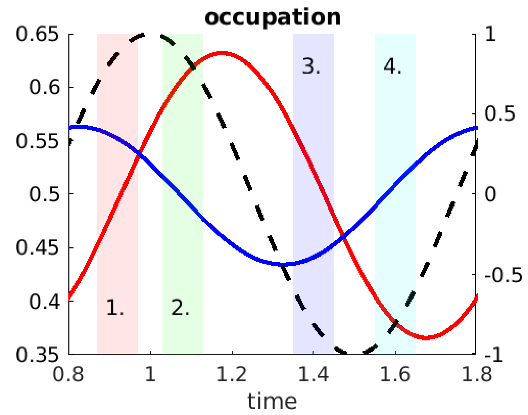
(a)

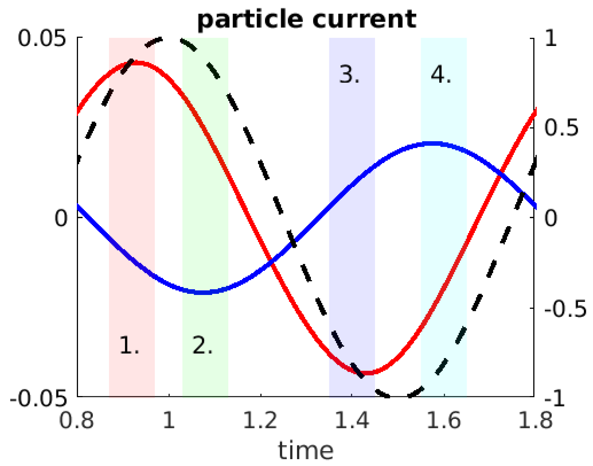
(b)

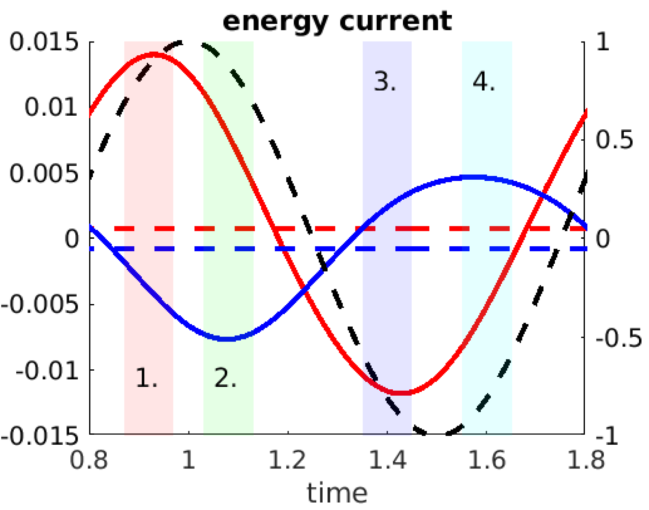
(c)

Figure 3: Observables measured over a period with driving of the left lead. Here, red lines correspond to the observables relating to the driven section, while blue lines refer to the undriven section of the model. Here, the energy current refers to the energy transfer from the lead and coupling region into the central region. The black dashed line is given by $\cos(\Omega t)$, while the colored dashed lines of Fig. 3(c) correspond to the averages of similarly colored energy currents. The parameters are $\Gamma_{\alpha}=\Gamma_{\beta}=0.5$, $U=0.6$, $T=0.001$, $\mu_{\alpha}=\mu_{\beta}=0.3$, $\epsilon_{A}=\epsilon_{B}=0$, $\Delta_{\alpha}=0.2$ and $\Omega=0.32$. The discretization was taken at $0.01$, the bounds of integration between $-40$ and $40$, and 49 Fourier coefficients were used. The convergence for both dots was taken as $10^{-4}$.

Taking real-time projections, we transform the equations of motion into matrix equations with the above transformations:

$$\begin{split}\left(\omega+\Omega m-\epsilon_{S}\right)\widetilde{G}_{S}^{R/A}\left(\omega,m,n\right)=\\ \delta_{mn}+\left[\widetilde{\Sigma}_{S}^{R/A}\circ\widetilde{G}_{S}^{R/A}\right]\left(\omega,m,n\right),\end{split}$$ (37)

$$\begin{split}\widetilde{G}_{S}^{<}(\omega,m,n)=\\ \left[\widetilde{G}_{S}^{R}\circ\widetilde{\Sigma}^{<}_{S}\circ\widetilde{G}_{S}^{A}\right]\left(\omega,m,n\right).\end{split}$$ (38)

The interaction self-energies can be cast in terms of Fourier coefficients: for GW,

$$\begin{split}\Sigma^{R/A}_{GW,S}\left(\omega,n\right)\\ =i\left[W_{S}^{ns,<}\;\square_{+}\;G^{R/A}_{S}+W_{S}^{ns,R/A}\;\square_{+}\;G^{>}_{S}\right]\left(\omega,n\right),\end{split}$$ (39)

$$\Sigma^{</>}_{GW,S}\left(\omega,n\right)=i\left[W_{S}^{ns,</>}\;\square_{+}\;G^{</>}_{S}\right]\left(\omega,n\right),$$ (40)

$$\begin{split}P_{S}^{R/A}(\omega,n)\\ =-i\left[G_{S}^{<}\;\square_{-}\;G^{A/R}_{S}+G_{S}^{R/A}\;\square_{-}\;G^{<}_{S}\right](\omega,n),\end{split}$$ (41)

$$\begin{split}P_{S}^{</>}(\omega,n)\\ =-i\left[G_{S}^{</>}\;\square_{-}\;G^{>/<}_{S}\right](\omega,n),\end{split}$$ (42)

$$\begin{split}\widetilde{W}_{S}^{ns,R/A}\left(\omega,m,n\right)=\widetilde{\Phi}^{R/A}_{S}\left(\omega,m,n\right)\\ +\left[\widetilde{\Phi}^{R/A}_{S}\circ\widetilde{P}^{R/A}_{S}\circ\widetilde{W}_{S}^{ns,R/A}\right]\left(\omega,m,n\right)\end{split}$$ (43)

and

$$\begin{split}\widetilde{W}_{S}^{ns,</>}\left(\omega,m,n\right)=\widetilde{\Phi}^{<\>}_{S}\left(\omega,m,n\right)\\ +\left[\widetilde{\Phi}^{R}_{S}\circ\widetilde{P}^{R}_{S}\circ\widetilde{W}_{S}^{ns,</>}\right]\left(\omega,m,n\right)\\ +\left[\widetilde{\Phi}^{R}_{S}\circ\widetilde{P}^{</>}_{S}\circ\widetilde{W}_{S}^{ns,A}\right]\left(\omega,m,n\right)\\ +\left[\widetilde{\Phi}^{</>}_{S}\circ\widetilde{P}^{A}_{S}\circ\widetilde{W}_{S}^{ns,A}\right]\left(\omega,m,n\right);\end{split}$$ (44)

for the particle-particle T-matrix,

$$\begin{split}\Sigma^{PP,R/A}_{S}\left(\omega,n\right)\\ =i\left[T^{PP,<}\;\square_{-}\;G^{A/R}_{\bar{S}}+T^{PP,R/A}\;\square_{-}\;G^{<}_{\bar{S}}\right]\left(\omega,n\right),\end{split}$$ (45)

$$\Sigma^{PP,</>}_{S}\left(\omega,n\right)=i\left[T^{PP,</>}\;\square_{-}\;G^{>/<}_{\bar{S}}\right]\left(\omega,n\right),$$ (46)

$$\begin{split}\widetilde{T}^{PP,R/A}\left(\omega,m,n\right)=-U\widetilde{G}^{H,R/A}\left(\omega,m,n\right)U\\ +U\left[\widetilde{G}^{H,R/A}\circ\widetilde{T}^{PP,R/A}\right](\omega,m,n),\end{split}$$ (47)

$$\begin{split}\widetilde{T}^{PP,</>}\left(\omega,m,n\right)=-U\widetilde{G}^{H,</>}\left(\omega,m,n\right)U\\ +U\left[\widetilde{G}^{H,R}\circ\widetilde{T}^{PP,</>}\right](\omega,m,n)\\ +U\left[\widetilde{G}^{H,</>}\circ\widetilde{T}^{PP,A}\right](\omega,m,n),\end{split}$$ (48)

$$\begin{split}G^{H,R/A}(\omega,n)\\ =i\left[G^{<}_{A}\;\square_{+}\;G^{R/A}_{B}+G^{R/A}_{A}\;\square_{+}\;G^{>}_{B}\right],(\omega,n),\end{split}$$ (49)

and

$$\begin{split}G^{H,</>}(\omega,n)\\ =i\left[G^{</>}_{A}\;\square_{+}\;G^{</>}_{B}\right](\omega,n);\end{split}$$ (50)

and for the particle-hole T-matrix,

$$\begin{split}\Sigma^{PH,R/A}_{S}\left(\omega,n\right)\\ =i\left[T_{S}^{PH,<}\;\square_{+}\;G^{R/A}_{\bar{S}}+T_{S}^{PH,R/A}\;\square_{+}\;G^{>}_{\bar{S}}\right]\left(\omega,n\right),\end{split}$$ (51)

$$\Sigma^{PH,</>}_{S}\left(\omega,n\right)=i\left[T_{S}^{PH,</>}\;\square_{+}\;G^{</>}_{\bar{S}}\right]\left(\omega,n\right),$$ (52)

$$\begin{split}\widetilde{T}_{S}^{PH,R/A}\left(\omega,m,n\right)=U\widetilde{G}_{S\bar{S}}^{F,R/A}\left(\omega,m,n\right)U\\ -U\left[\widetilde{G}_{S\bar{S}}^{F,R/A}\circ\widetilde{T}^{PH,R/A}_{S}\right](\omega,m,n),\end{split}$$ (53)

$$\begin{split}\widetilde{T}_{S}^{PH,</>}\left(\omega,m,n\right)=U\widetilde{G}_{S\bar{S}}^{F,</>}\left(\omega,m,n\right)U\\ -U\left[\widetilde{G}_{S\bar{S}}^{F,</>}\circ\widetilde{T}^{PH,A}_{S}\right](\omega,m,n)\\ -U\left[\widetilde{G}_{S\bar{S}}^{F,R}\circ\widetilde{T}^{PH,</>}_{S}\right](\omega,m,n),\end{split}$$ (54)

$$\begin{split}G_{S\bar{S}}^{F,R/A}(\omega,n)\\ =-i\left[G^{<}_{S}\;\square_{-}\;G^{A/R}_{\bar{S}}+G^{R/A}_{S}\;\square_{-}\;G^{<}_{\bar{S}}\right](\omega,n),\end{split}$$ (55)

and

$$\begin{split}G_{S\bar{S}}^{F,</>}(\omega,n)\\ =-i\left[G^{</>}_{S}\;\square_{-}\;G^{>/<}_{\bar{S}}\right](\omega,n).\end{split}$$ (56)

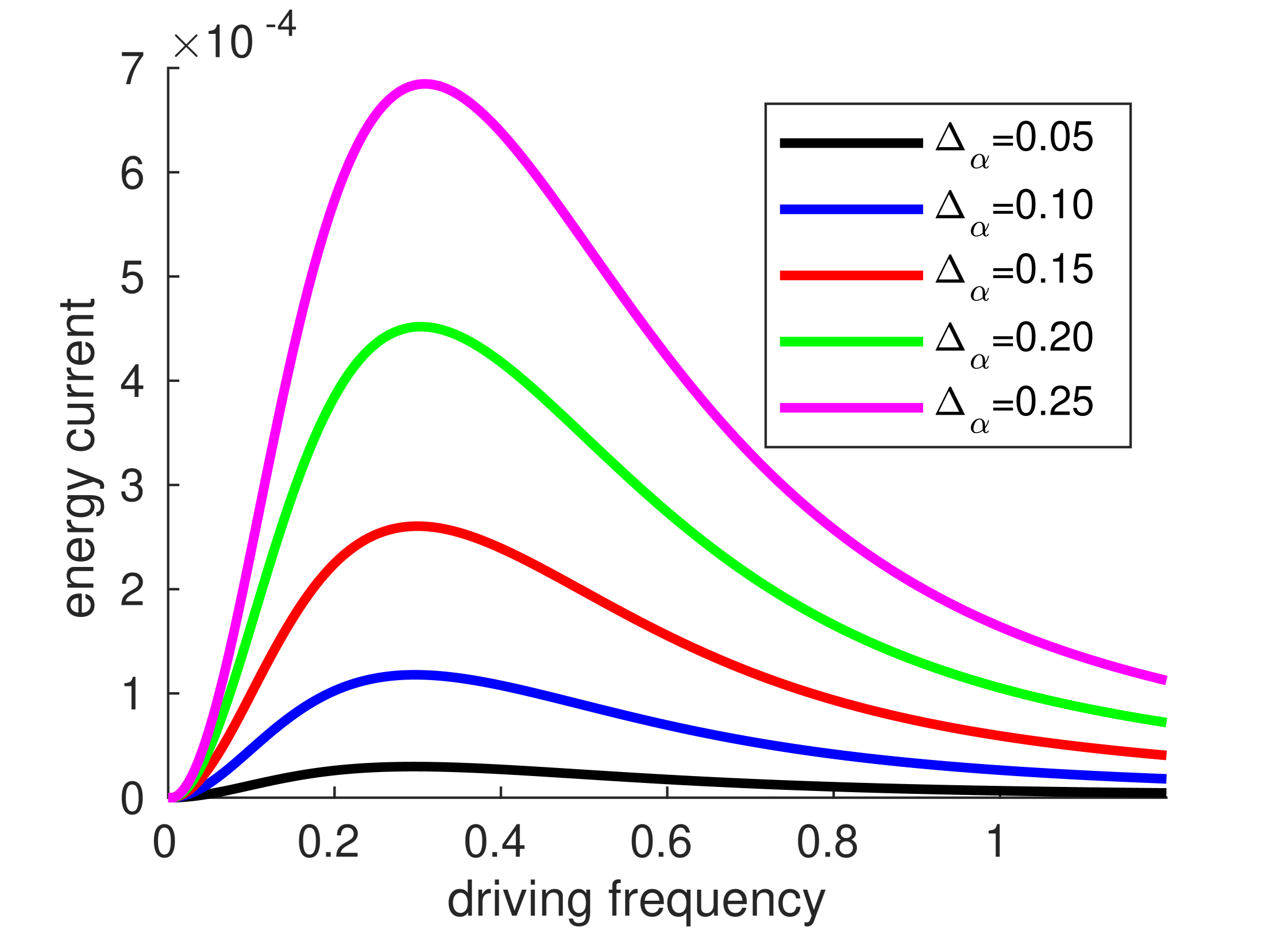
(a)

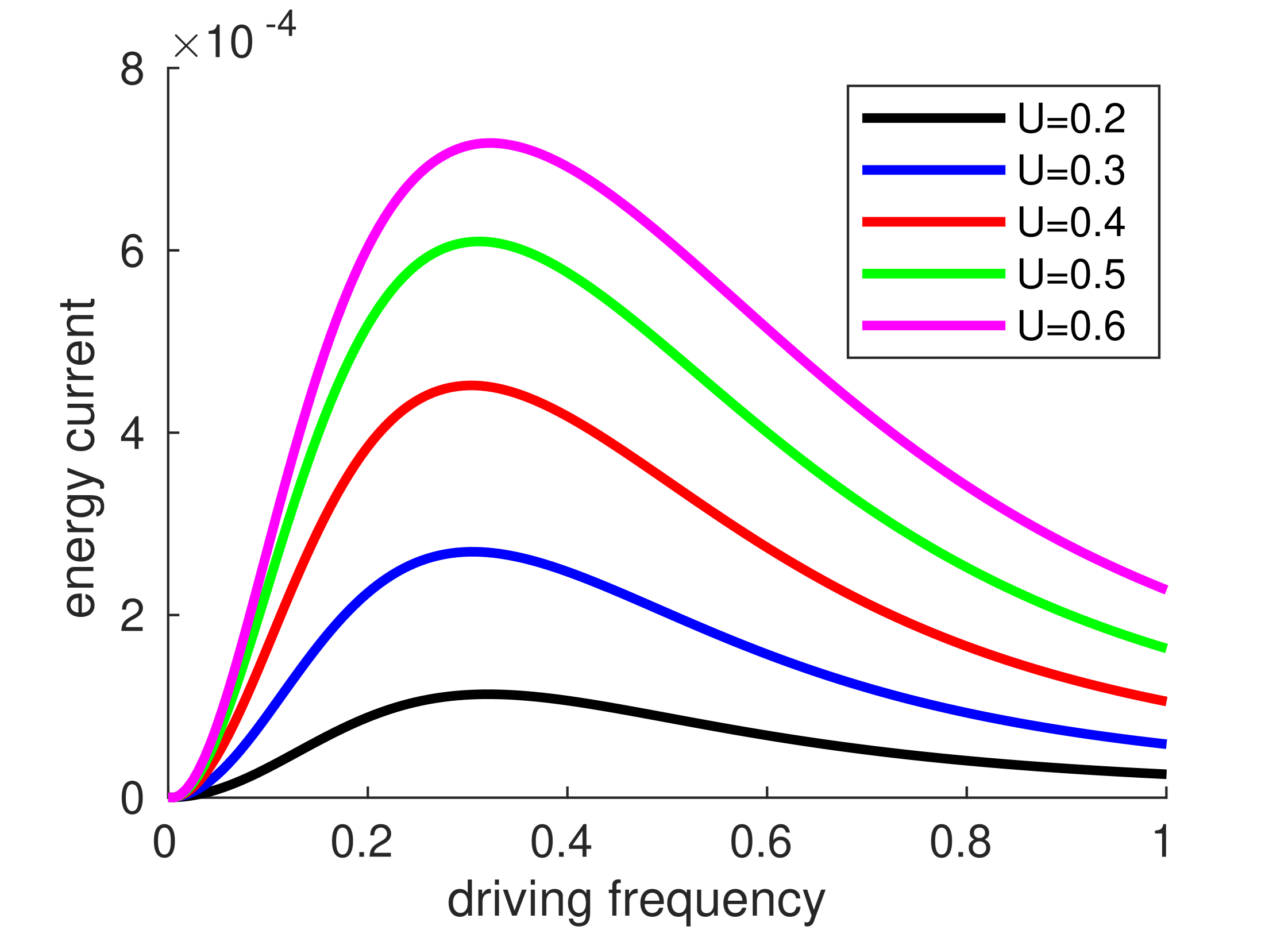
(b)

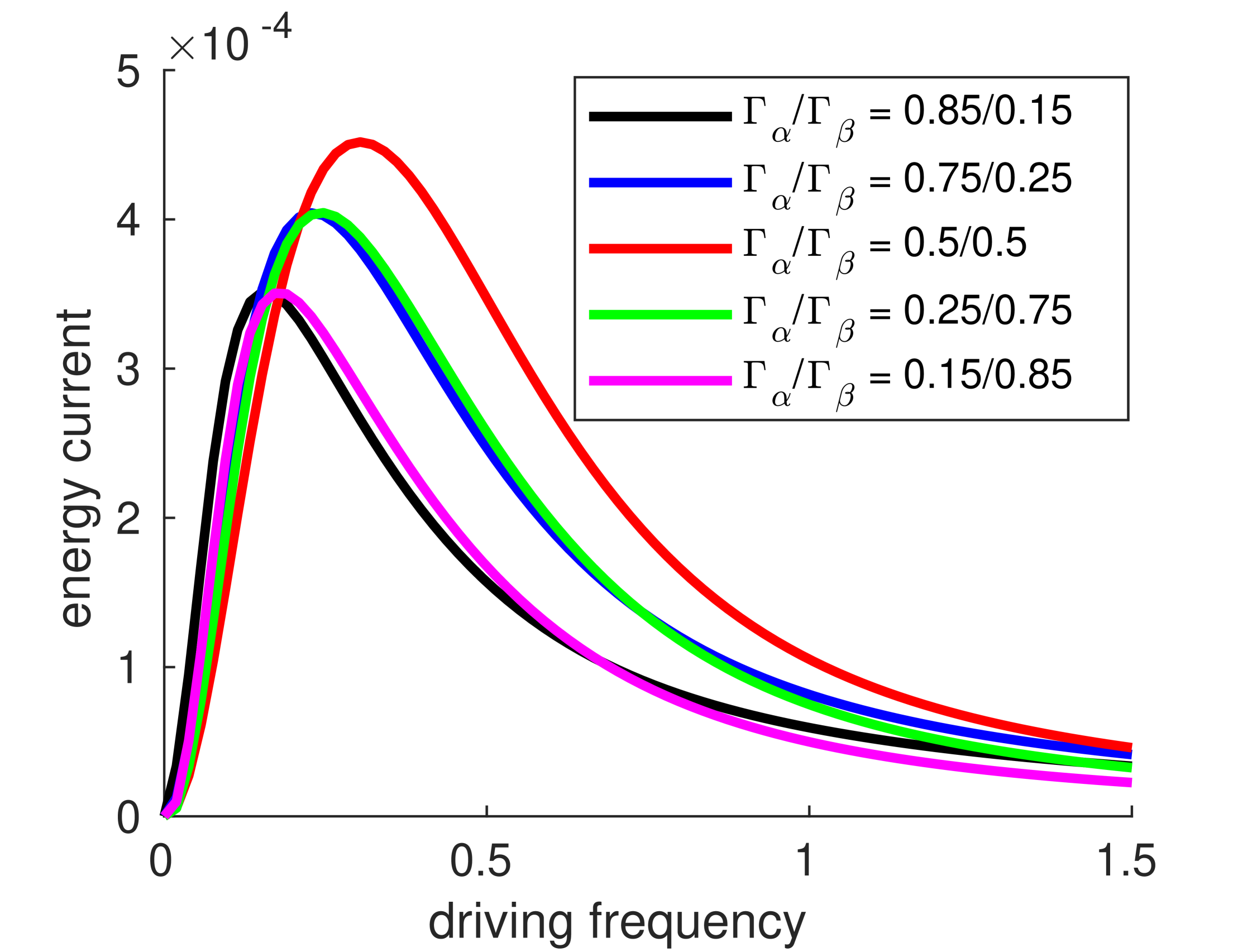
(c)

Figure 4: Time-averaged energy current through the system due to the periodic driving of the left lead. The parameters, unless specified, are $\Gamma_{\alpha}=\Gamma_{\beta}=0.5$, $\epsilon_{A}=\epsilon_{B}$=-0.2, $U=0.4$, $T=0.001$, $\mu_{\alpha}=\mu_{\beta}=0$ and $\Delta_{\alpha}=0.2$. The discretization was taken at $0.01$, the bounds of integration between $-40$ and $40$, and 49 Fourier coefficients were used. The convergence for both dots was taken as $10^{-4}$

The time-dependent driving of the leads’ energies was taken as sinusoidal,

$$\psi_{\alpha}(t)=\Delta_{\alpha}\cos(\Omega t),$$ (57)

giving $\Psi_{\alpha}(t)=\left(\Delta_{\alpha}/\Omega\right)\sin\left(\Omega t\right)$, which can be expanded with the Jacobi-Anger expansion

$$e^{i\frac{\Delta_{\alpha}}{\Omega}\sin(\Omega t)}=\sum_{n=-\infty}^{n=\infty}J_{n}\left(\frac{\Delta_{\alpha}}{\Omega}\right)e^{in\Omega t},$$ (58)

where $J_{n}(x)$ are Bessel functions of the first kind. We can recast equation (21), as a Floquet matrices,

$$\bar{\Sigma}_{\sigma}\left(\omega,m,n\right)=\left[\widetilde{S}_{\sigma}\circ{\widetilde{\Sigma}^{\prime}}_{\sigma}\circ{\widetilde{S}_{\sigma}}^{\dagger}\right]\left(\omega,m,n\right),$$ (59)

where $\widetilde{S}_{\sigma}\left(m,n\right)=J_{m-n}\left(\Delta_{\sigma}/\Omega\right)$.

In a similar manner to the equations of motion, the observables can be cast in terms of Fourier coefficients:

$$\begin{split}I^{P}_{\sigma}(n-m)=\widetilde{I}^{P}_{\sigma}\left(m,n\right)\\ =2\int^{\infty}_{-\infty}\frac{d\omega}{2\pi}\;\left[\widetilde{G}_{S}^{R}\circ\widetilde{\Sigma}^{<}_{\sigma}+\widetilde{G}_{S}^{<}\circ\widetilde{\Sigma}^{A}_{\sigma}\right](\omega,m,n),\end{split}$$ (60)

$$\begin{split}n_{S}\left(n-m\right)=\widetilde{n}_{S}\left(m,n\right)=-i\int^{\infty}_{-\infty}\frac{d\omega}{2\pi}\widetilde{G}_{S}^{<}(\omega,m,n),\end{split}$$ (61)

and

$$\begin{split}I^{E}_{\sigma}(n-m)=\widetilde{I}^{E}_{\sigma}\left(m,n\right)\\ =-2\int^{\infty}_{-\infty}\frac{d\omega}{2\pi}\;\left(\omega+m\Omega\right)\left[\widetilde{\Sigma}_{\sigma}^{<}\circ\widetilde{G}^{A}_{S}+\widetilde{\Sigma}_{\sigma}^{R}\circ\widetilde{G}^{<}_{S}\right](\omega,m,n).\end{split}$$ (62)

II.3 Implementation

To solve the equations of motion, we invert equations (37),(43),(44),(47),(48),(53) and (54) by first truncating the Floquet matrices, as defined in Eq. (35). Equations (39), (40), (41), (42),(45), (46), (49), (50), (51), (52), (55) and (56) are calculated by using the Fourier coefficient taken from the appropriate Floquet matrices. These Fourier coefficients were taken from the terms of the Floquet matrices given by $n+m=0,-1$ of equation (35). The self-energy terms were then transformed back to Floquet matrix form, using equation (35), for use in the equations of motion. The self-consistent process begins with calculating the noninteracting case followed by the interaction self-energies, as specified above. The interaction self-energies are then used to calculate successive iterations of the Green’s functions before the following convergence is satisfied:

$$\begin{split}\frac{\sum_{m}\left|n_{m}^{k}-n_{m}^{k-1}\right|}{\sum_{m}\left|n^{k}_{m}\right|}\leq\delta,\end{split}$$ (63)

where $n^{k}_{m}$ is the $k$th iteration of the $m$th Fourier coefficent of the occupation in question, with $\delta$ as the convergence. This convergence was satisfied for each dot’s occupation.

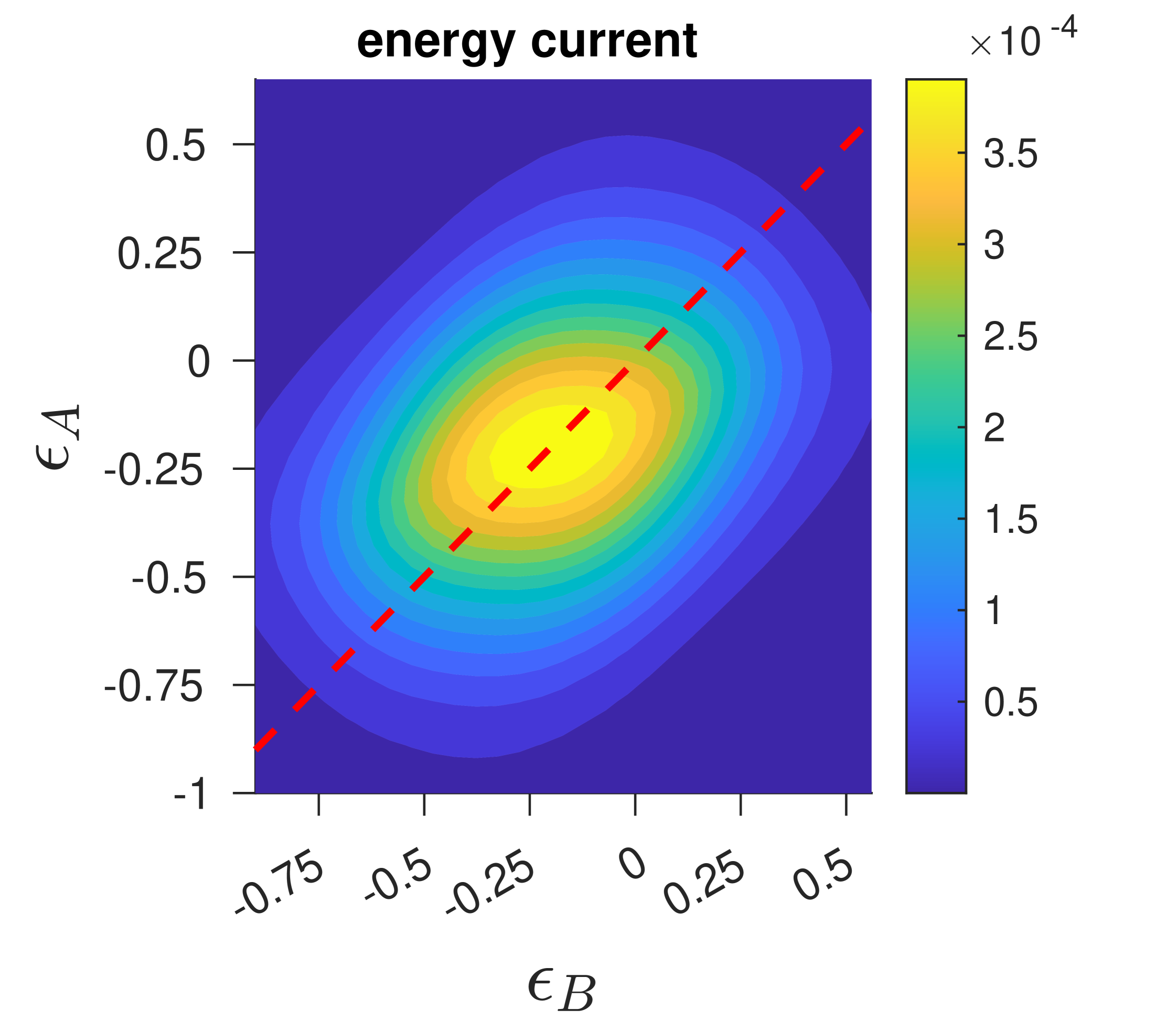
(a)

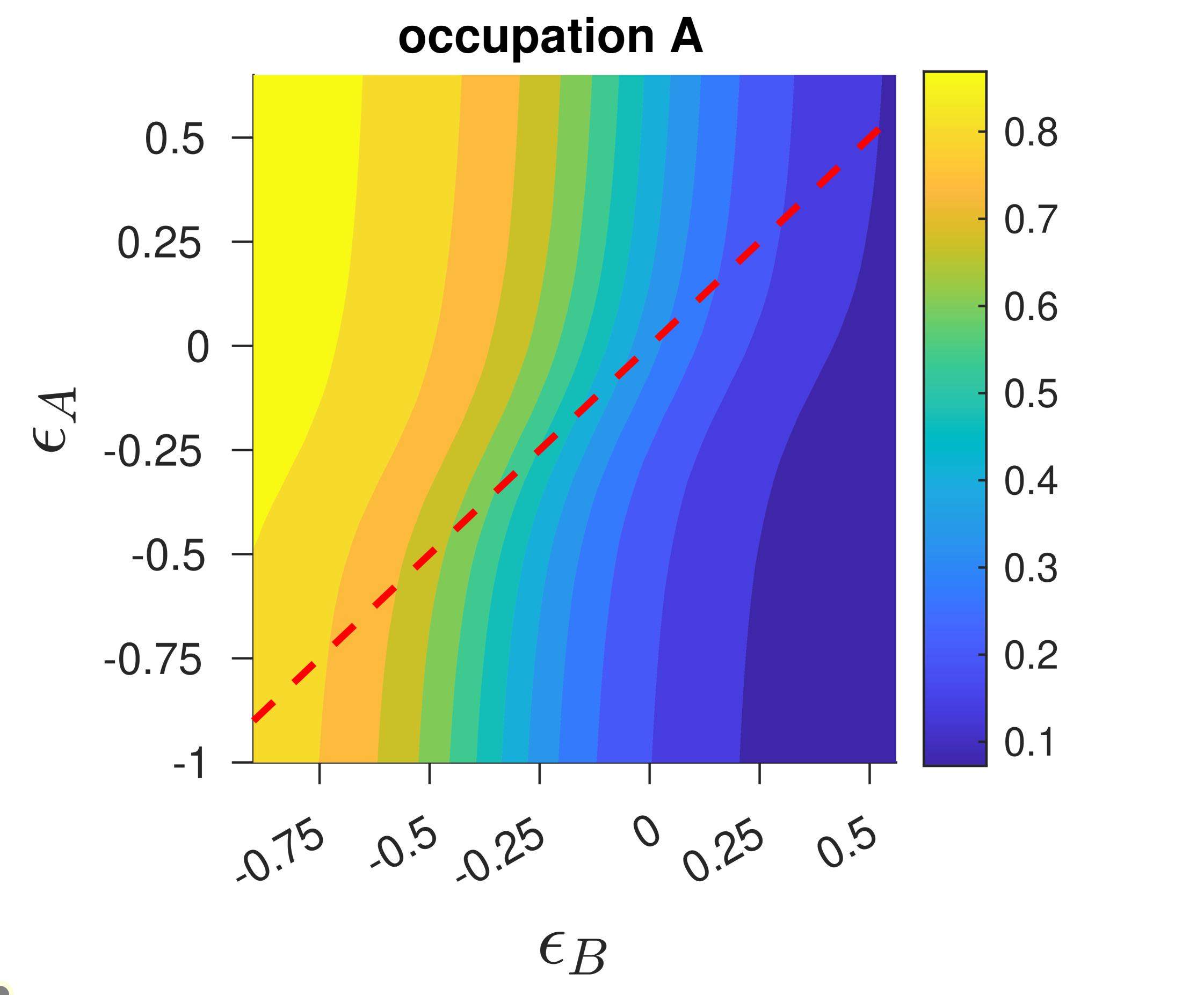
(b)

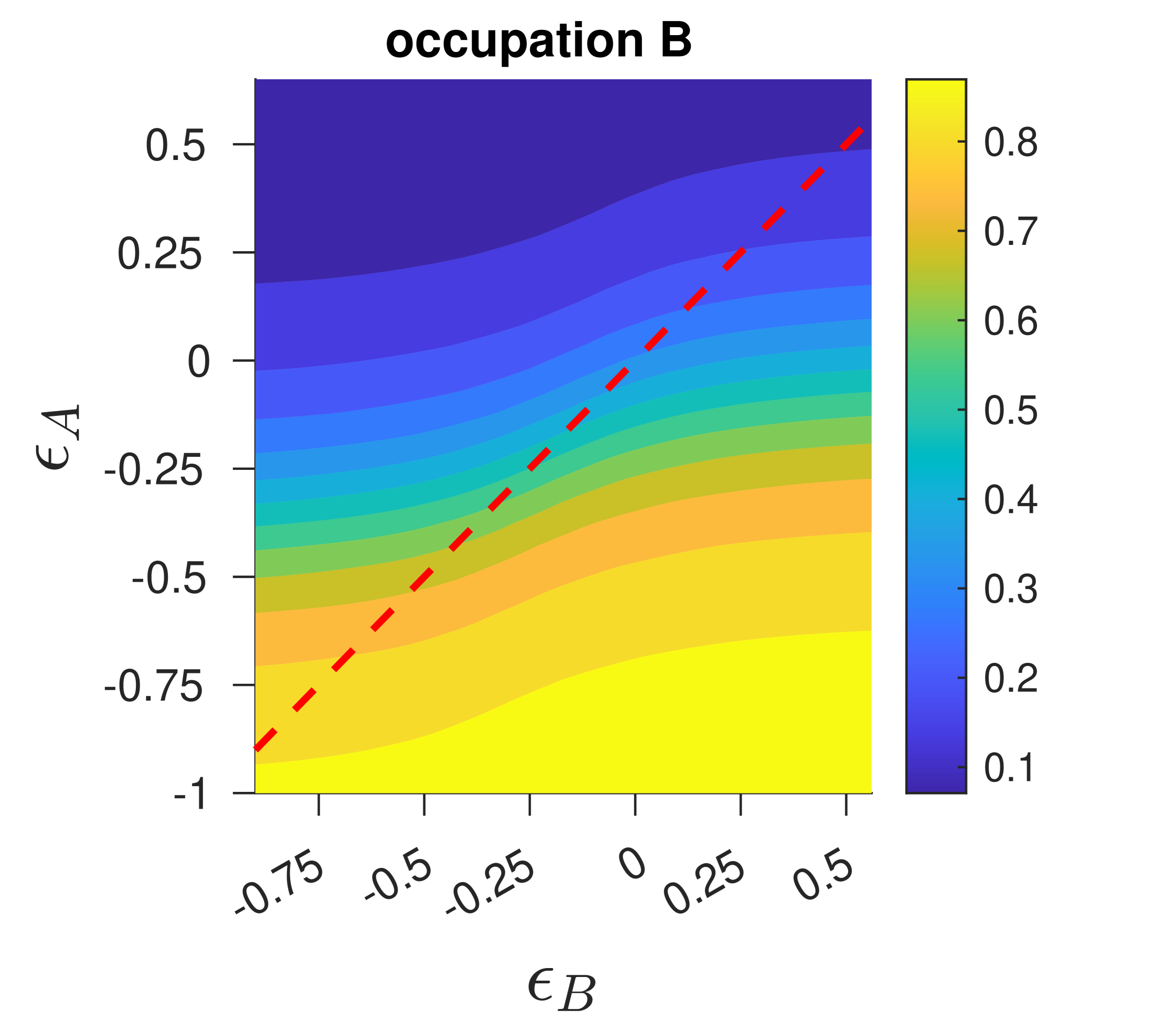
(c)

Figure 5: Time-averaged observables through the system, with driving of the left lead. The parameters are $\Gamma_{\alpha}=\Gamma_{\beta}=0.5$, $U=0.4$, $T=0.001$, $\mu_{\alpha}=\mu_{\beta}=0$, $\Delta_{\alpha}=0.2$ and $\Omega=0.4$. The discretization was taken at $0.01$, the bounds of integration between $-40$ and $40$ and 49 Fourier coefficients were used. The convergence for both dots was taken as $10^{-4}$. The red dashed line follows $\epsilon_{A}=\epsilon_{B}$.

III Results and Discussion

Within the system, energy moves from the driven to the undriven section via the capacitive coupling of the two dots. In particular, energy transfer occurs when the driven dot is occupied at a higher energy and unoccupied at a lower energy, and the undriven dot is unoccupied at a higher energy and occupied at a lower energy. This process is complicated because the energies at which a dot is occupied are informed by the occupation of the opposing dot. This relationship is transparent in the Hartree approximation, where the average energy current into the central region due to current into the dot $S$ is given by

$$\bar{I^{E}_{\sigma}}=U\int^{P}_{0}\frac{dt}{P}\;n_{\bar{S}}(t)I^{P}_{\sigma}(t).$$ (64)

These observations, coupled with the sinusoidal nature of the driving, suggest the following approximate cyclic stages in the energy transfer process:

1. Following stage $4$, charge moves onto the driven dot while the undriven dot is largely occupied.

2. The driven dot is largely occupied as charge moves off the undriven dot.

3. Charge moves off the driven dot as the undriven dot is largely unoccupied.

4. The driven dot is largely unoccupied as charge moves onto the undriven dot.

Stages one and two capture the movement of higher energy electrons moving onto the driven dot and off the undriven dot, resulting in the energy transfer from the driven to the undriven region. Stages three and four capture the lower energy electrons moving off the driven dot and onto the undriven dot, resulting in a lower energy transfer than the first two steps in the cycle in the opposite direction. An example of this can be seen in Fig. 3, where the regions in which the stages are most prominent have been highlighted.

The amount of energy transferred through the system is sensitive to the driving frequency, with the maximum transference a result of the balancing of stages of energy transfer [see in Fig. 4]. As the driving frequency decreases, electrons move between the dots and their respective leads quicker than the energy transfer stages can complete. In particular, the dots that remain largely occupied in stages one and two and largely unoccupied in processes three and four begin to change in occupation, resulting in less pronounced changes in the opposing dot’s occupation energy and outgoing energy current. Conversely, as the driving frequency increases, the charge has less time to move between the dots and their respective leads, resulting in smaller maxima and minima for the occupations over the period, which reduces the opposing dot’s occupation energy and its outgoing energy current.

The driving profile and the system parameters beyond the driving frequency also inform the effectiveness of the energy transfer process. As expected, given Eq. (64), increases in the interaction strength $U$ were found to increase the average energy current through the system [see Fig. 4(b)]. It was also found that significant asymmetry of the coupling strengths diminished energy flow through the system [see Fig. 4(c)]. This is due to uneven transfer rates, $\tau_{\sigma}\sim 1/\Gamma_{\sigma}$, for the movement of electrons between the dots and their respective leads, resulting in the inefficient completion of the stages of the energy transfer process. For the energies of the dots, the largest transference of energy through the system was achieved with dots with equal energies situated below the chemical potential of the two leads, such that, on average, the dots are both around half filled [see Fig. 5].

IV Conclusion

We have investigated two capacitively coupled quantum dots coupled to respective leads, where one lead’s energies are driven sinusoidally. While particles cannot move between the dots, Coulomb repulsion between the dots allows for the transfer of energy. The stages of the energy transfer were identified, and the effects of system parameters’ were investigated. In particular, it was found that energy transfer was maximized for a given driving, corresponding to the efficient completion of the identified energy transfer process.

This work has focused on a regime of relatively weak coupling with $\Gamma>U$. Further work in a regime of $\Gamma<U$ may result in different energy transfer stages, as outlined in Sec. III, for various drivings, suggesting interesting possible avenues for further research. Moreover, more complicated driving profiles and statistics relating to energy transfer may prove valuable in understanding and manipulating energy transfer in systems like that investigated.

This result furthers the understanding of particle and energy transfer in capacitively coupled quantum dots, particularly within the context of nonadiabatic driving. This is particularly important as the miniaturization of nanoelectronics brings active elements closer together, resulting in the potential for unwarranted capacitive coupling.

References

• [1] A. J. Keller, J. S. Lim, David Sánchez, Rosa López, S. Amasha, J. A. Katine, Hadas Shtrikman, and D. Goldhaber-Gordon. Cotunneling drag effect in coulomb-coupled quantum dots. Phys. Rev. Lett., 117:066602, Aug 2016.
• [2] Miguel A. Sierra, David Sánchez, Antti-Pekka Jauho, and Kristen Kaasbjerg. Fluctuation-driven coulomb drag in interacting quantum dot systems. Phys. Rev. B, 100:081404(R), Aug 2019.
• [3] Ludovico Tesser, Bibek Bhandari, Paolo Andrea Erdman, Elisabetta Paladino, Rosario Fazio, and Fabio Taddei. Heat rectification through single and coupled quantum dots. New Journal of Physics, 24(3):035001, mar 2022.
• [4] A. A. Aligia, D. Pérez Daroca, Liliana Arrachea, and P. Roura-Bas. Heat current across a capacitively coupled double quantum dot. Phys. Rev. B, 101:075417, Feb 2020.
• [5] Hari Kumar Yadalam and Upendra Harbola. Statistics of heat transport across a capacitively coupled double quantum dot circuit. Phys. Rev. B, 99:195449, May 2019.
• [6] A.-M. Daré. Comparative study of heat-driven and power-driven refrigerators with coulomb-coupled quantum dots. Phys. Rev. B, 100:195427, Nov 2019.
• [7] Rafael Sánchez and Markus Büttiker. Optimal energy quanta to current conversion. Phys. Rev. B, 83:085428, Feb 2011.
• [8] Holger Thierschmann, Rafael Sánchez, Björn Sothmann, Fabian Arnold, Christian Heyn, Wolfgang Hansen, Hartmut Buhmann, and Laurens W. Molenkamp. Three-terminal energy harvester with coupled quantum dots. Nature Nanotechnology, 10(10):854–858, Oct 2015.
• [9] Björn Sothmann, Rafael Sánchez, and Andrew N Jordan. Thermoelectric energy harvesting with quantum dots. Nanotechnology, 26(3):032001, dec 2014.
• [10] Nicklas Walldorf, Antti-Pekka Jauho, and Kristen Kaasbjerg. Thermoelectrics in coulomb-coupled quantum dots: Cotunneling and energy-dependent lead couplings. Phys. Rev. B, 96:115415, Sep 2017.
• [11] María Florencia Ludovico, Liliana Arrachea, Michael Moskalets, and David Sánchez. Periodic energy transport and entropy production in quantum electronics. Entropy, 18(11), 2016.
• [12] María Florencia Ludovico, Michael Moskalets, David Sánchez, and Liliana Arrachea. Dynamics of energy transport and entropy production in ac-driven quantum electron systems. Phys. Rev. B, 94:035436, Jul 2016.
• [13] María Florencia Ludovico, Jong Soo Lim, Michael Moskalets, Liliana Arrachea, and David Sánchez. Time resolved heat exchange in driven quantum systems. Journal of Physics: Conference Series, 568(5):052017, dec 2014.
• [14] A.-M. Daré and P. Lombardo. Time-dependent thermoelectric transport for nanoscale thermal machines. Phys. Rev. B, 93:035303, Jan 2016.
• [15] María Florencia Ludovico and Massimo Capone. Enhanced performance of a quantum-dot-based nanomotor due to coulomb interactions. Phys. Rev. B, 98:235409, Dec 2018.
• [16] Stefan Juergens, Federica Haupt, Michael Moskalets, and Janine Splettstoesser. Thermoelectric performance of a driven double quantum dot. Phys. Rev. B, 87:245423, Jun 2013.
• [17] Jong Soo Lim, Rosa López, and David Sánchez. Dynamic thermoelectric and heat transport in mesoscopic capacitors. Phys. Rev. B, 88:201304(R), Nov 2013.
• [18] Jian Chen, Minhui ShangGuan, and Jian Wang. A gauge invariant theory for time dependent heat current. New Journal of Physics, 17(5):053034, may 2015.
• [19] María Florencia Ludovico and Massimo Capone. Charge and energy transfer in ac-driven coulomb-coupled double quantum dots. The European Physical Journal B, 95(6):99, Jun 2022.
• [20] Tobias Brandes. Truncation method for green’s functions in time-dependent fields. Phys. Rev. B, 56:1213–1224, Jul 1997.
• [21] Thomas D. Honeychurch and Daniel S. Kosov. Full counting statistics for electron transport in periodically driven quantum dots. Phys. Rev. B, 102:195409, Nov 2020.
• [22] Thomas D. Honeychurch and Daniel S. Kosov. Quantum transport in driven systems with vibrations: Floquet nonequilibrium green’s functions and the self-consistent born approximation. Phys. Rev. B, 107:035410, Jan 2023.
• [23] Patrick Haughian, Han Hoe Yap, Jiangbin Gong, and Thomas L. Schmidt. Charge pumping in strongly coupled molecular quantum dots. Phys. Rev. B, 96:195432, Nov 2017.
• [24] Hideo Aoki, Naoto Tsuji, Martin Eckstein, Marcus Kollar, Takashi Oka, and Philipp Werner. Nonequilibrium dynamical mean-field theory and its applications. Rev. Mod. Phys., 86:779–837, Jun 2014.
• [25] N Schlünzen, S Hermanns, M Scharnke, and M Bonitz. Ultrafast dynamics of strongly correlated fermions—nonequilibrium green functions and selfenergy approximations. Journal of Physics: Condensed Matter, 32(10):103001, dec 2019.