Generative Prompt Model for Weakly Supervised Object Localization

Abstract

Weakly supervised object localization (WSOL) remains challenging when learning object localization models from image category labels. Conventional methods that discriminatively train activation models ignore representative yet less discriminative object parts. In this study, we propose a generative prompt model (GenPromp), defining the first generative pipeline to localize less discriminative object parts by formulating WSOL as a conditional image denoising procedure. During training, GenPromp converts image category labels to learnable prompt embeddings which are fed to a generative model to conditionally recover the input image with noise and learn representative embeddings. During inference, GenPromp combines the representative embeddings with discriminative embeddings (queried from an off-the-shelf vision-language model) for both representative and discriminative capacity. The combined embeddings are finally used to generate multi-scale high-quality attention maps, which facilitate localizing full object extent. Experiments on CUB-200-2011 and ILSVRC show that GenPromp respectively outperforms the best discriminative models by 5.2% and 5.6% (Top-1 Loc), setting a solid baseline for WSOL with the generative model. Code is available at https://github.com/callsys/GenPromp.

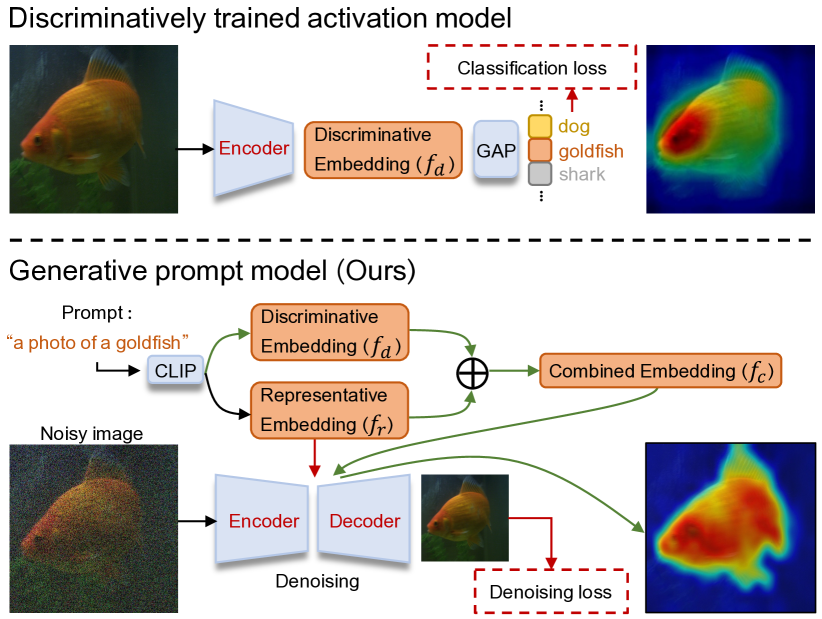
Figure 1: Comparison of our generative prompt model (GenPromp) with the discriminatively trained activation model. GenPromp aims to localize less discriminative object parts by formulating WSOL as a conditional image denoising procedure. Red, green, and black arrows respectively denote information propagation during training, inference, and training $\&$ inference. $f_{d}$, $f_{r}$, and $f_{c}$ denote the discriminative, representative, and combined embeddings.

1 Introduction

Weakly supervised object localization (WSOL) is a challenging task when provided with image category supervision but required to learn object localization models. As a pioneered WSOL method, Class Activation Map (CAM) [75] defines global average pooling (GAP) to generate semantic-aware localization maps based on a discriminatively trained activation model. Such a fundamental method, however, suffers from partial object activation while often missing full object extent, Fig. 1(upper). The nature behind the phenomenon is that discriminative models are born to pursue compact yet discriminative features while ignoring representative ones [3, 22].

Many efforts have been proposed to alleviate the partial activation issue by introducing spatial regularization terms [36, 38, 39, 60, 67, 24, 68, 73, 74], auxiliary localization modules [38, 41, 62, 63], or adversarial erasing strategies [13, 14, 39, 73]. Nevertheless, the fundamental challenge about how to use a discriminatively trained classification model to generate precise object locations remains.

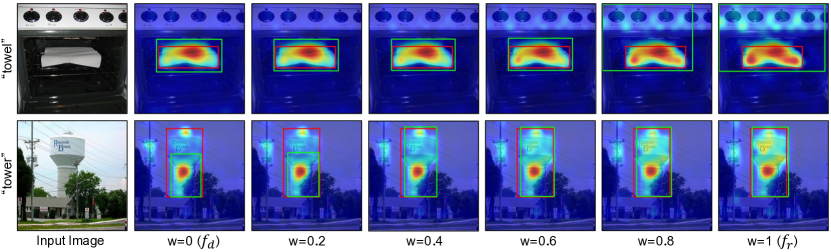
Figure 2: Activation maps and localization results using discriminative and representative embeddings. A proper combination ($w$=0.6) of discriminative embeddings $f_{d}$ with representative embedding $f_{r}$ as the prompt produces precise activation maps and good WSOL results (green boxes).

In this study, we propose a generative prompt model (GenPromp), Fig. 1(lower), which formulates WSOL as a conditional image denoising procedure, solving the fundamental partial object activation problem in a new and systematic way. During training, for each category (e.g.goldfish in Fig. 1) in the predetermined category set, GenPromp converts each category label to a learnable prompt embedding ($f_{r}$) through a pre-trained vision-language model (CLIP) [47]. The learnable prompt embedding is then fed to a transformer encoder-decoder to conditionally recover the noisy input image. Through multi-level denoising, the representative features of input images are back-propagated from the transformer decoder to the learnable prompt embedding, which is updated to the representative embedding $f_{r}$.

During inference, GenPromp linearly combines learned representative embeddings ($f_{r}$) with discriminative embeddings ($f_{d}$) to obtain both object generative and discrimination capability, Fig. 2. $f_{d}$ is queried from a pre-trained vision-language model (CLIP), which incorporates the correspondence between text (e.g.category labels) with vision feature embeddings. The combined embedding ($f_{c}$) is used to generate attention maps at multiple levels and timestamps, which are aggregated to object activation maps through a post-processing strategy. On CUB-200-2011 [56] and ImageNet-1K [52], GenPromp respectively outperforms the best discriminative models by 5.2% (87.0% $vs.$ 81.8% [63]) and 5.6% (65.2% $vs.$ 59.6% [63]) in Top-1 Loc.

The contributions of this study include:

• We propose a generative prompt model (GenPromp), providing a systematic way to solve the inconsistency between the discriminative models with the generative localization targets by formulating a conditional image denoising procedure.

• We propose to query discriminative embeddings from an off-the-shelf vision-language model using image labels as input. Combining the discriminative embeddings with the generative prompt model facilitates localizing objects while depressing backgrounds.

• GenPromp significantly outperforms its discriminative counterparts on commonly used benchmarks, setting a solid baseline for WSOL with generative models.

2 Related Work

Weakly Supervised Object Localization. As a simple-yet-effective method, CAM [75] localizes objects by introducing global average pooling (GAP) to an image classification network. CAM is also extended from WSOL to weakly supervised detection [12, 57, 70] and segmentation  [10, 58, 63, 71]. However, CAM suffers from partial activation, $i.e.$, activating the most discriminative parts instead of full object extent. The reason lies in the inconsistency between the discriminative models ($i.e.$, classification model) with the generative target (object localization).

To solve the partial activation problem, adversarial erasing, discrepancy learning, online localization refinement, classifier-localizer decoupling, and attention regularization methods are proposed. As a spatial regularization method, adversarial erasing [13, 14, 39, 55, 68, 73] online removes significantly activated regions within feature maps to drive learning the missed object parts. With a similar idea, spatial discrepancy learning [23, 67] leverages adversarial classifiers to enlarge object areas. Through classifier-localizer decoupling, PSOL [69] partitions the WSOL pipeline into two parts: class-agnostic object localization and object classification. For class-agnostic localization, it uses class-agnostic methods to generate noisy pseudo annotations and then perform bounding box regression on them without class labels. While online refinement of low-level features improves activation maps for WSOL [62], BAS [60] specifies a background activation suppression strategy to assist the learning of WSOL models. C²AM [63] generates class-agnostic activation maps using contrastive learning without category label supervision. FAM [41] optimizes the object localizer and classifiers jointly via object-aware and part-aware attention modules. TS-CAM [22] and LCTR [11] utilize the attention maps defined on long-range feature dependency of transformers to localize objects.

Despite the progress, existing methods typically ignore the fundamental challenge of WSOL, $i.e.$ discriminative models are required to perform representative (localization) tasks.

Vision-Language Models. Vision-language models have demonstrated increasing importance for vision tasks. In the early years, great efforts are paid to label image-text pairs which are important for vision-language model training [8, 16, 49, 66]. In recent years, the born-ed association relations of image and text on the Web facilitate collecting a massive quantity of image-text pairs [7, 43, 47, 53, 54], which requires much lower annotation cost compared to those manually annotated datasets (See supplementary for details). Such image-text pairs enable building the association between image category labels and visual feature embedding, which is the foundation of this study. Based on the massive quantity of image-text pairs, we pre-train two components of GenPromp (i.e.Stable diffusion [50], CLIP [47]) with two large image-text pair datasets. In specific, we pre-train the image denoising model using LAION-5B [53] and the CLIP model on WIT  [47].

Generative Vision Models. As the foundation of most generative vision models, GAN [25] defines an adversarial training process, where it simultaneously trains a generative model and a discriminative model. Many efforts have been made to improve GAN such as better optimization strategies [2, 26, 40, 44, 64], conditional image generation [31, 33, 34] and improved architecture [6, 32, 48, 72]. Recently, a generative vision paradigm, $i.e.$, denoising diffusion probabilistic models (DDPM) [30] become popular and have the potential to surpass GAN in several vision generation tasks such as image generation [18, 21, 46, 50, 51] and image editing [29, 35]. DDPM have also been adapted to some perception tasks such as object detection [9] and image segmentation [1, 5, 61], which inspires this study for WSOL.

Viewing categories labels as prompt embeddings is an important feature of GenPromp, which originates from conditional image generation tasks. This follows DDPM which feeds a language description encoded by the language model (e.g.BERT [17]) to the generative model for sematic-aware image generation. Existing works [21, 29, 35, 51] have proposed to learn the representative embeddings from user-provided images that contains a new object or a new style, which drive DDPM to generate synthesis images that contains that object or style. Inspired by this learning paradigm, GenPromp is proposed to learn the representative embeddings of each category, which are crucial for object localization.

3 Preliminaries

Diffusion models learn a data distribution $p(x)$ by gradually denoising a normally distributed variable, which corresponds to learning a reverse process of a Markov Chain [30]. Stable diffusion [50] leverages well-trained perceptual compression model $\mathcal{E}$ to transfer the denoising diffusion process from the high-dimensional pixel space to a low-dimensional latent space, which reduces the computational burden and increases efficiency. The objective function of Stable diffusion is defined as

$$\mathcal{L}(\theta,f) =\mathbb{E}_{x,\epsilon,t}\Big{[}||\epsilon-\epsilon_{\theta}(z_{t},t,f)||^{2}_{2}\Big{]},$$ (1)

$$z_{t} =\sqrt{\overline{\alpha}_{t}}\mathcal{E}(x)+\sqrt{1-\overline{\alpha}_{t}}\epsilon,t\in T,$$ (2)

where $\epsilon\sim N(0,1)$ is sampled from the normal distribution and $\epsilon_{\theta}(\circ,t,f)$ is the neural backbone, which is implemented as an attention-unet conditioned on time $t$ and the prompt embedding $f$. $\mathcal{E}$ is implemented as a VQGAN [20] encoder. $z_{t}$ is the noisy latent of the input image $x$ at time $t,t\in T=\{1,2,\cdots,1000\}$. $\{\overline{\alpha}_{t}\}_{t\in T}$ denotes a set of hyperparameters that steer the levels of noise added.

4 Generative Prompt Model

GenPromp consists of a training stage (Fig. 3) and a finetuning stage. In the training stage, the discriminative embedding $f_{d}$ is queried from a pre-trained CLIP model (Querying Discriminative Embeddings), meanwhile a representative embedding $f_{r}$ is specified for each category (Learning Representative Embedding.). In the finetuning stage, $f_{d}$ and $f_{r}$ are used to prompt the backbone network finetuning (Model Finetuning). The trained models and combined prompt embeddings (Combining Embeddings) are used to predict attention maps for WSOL (Fig. 4).

Querying Discriminative Embeddings. The embedding $f_{d}$ is queried from a pre-trained CLIP model [47], which uses a prompt string ($p$) as input and outputs a language feature vector. As CLIP is pre-trained with a discriminative loss ($i.e.$, contrastive loss), $f_{d}$ is therefore discriminative.

During training, for a given category (e.g.goldfish in Fig. 3), the prompt is obtained by filling the category label string to a template (e.g.“a photo of a goldfish”). During inference, however, the image category labels are unavailable. An intuitive way is using a pre-trained classifier to predict the category of the input image. Unfortunately, some category labels correspond to strings of multiple words, which imply multiple tokens and multiple attention maps. Such multiple attention maps with noise would deteriorate the localization performance. To address this issue, we heuristically select the last token of the first string to initialize the prompt, which is referred to as the meta token. For example, we select goldfish for category string “goldfish, Carassius auratus” and select ray for category string “electric ray, crampfish, numbfish, torpedo”. The meta token of a category is typically the name of its superclass.

To query discriminative embedding $f_{d}$ from the CLIP model, the prompt $p$ is converted to an ordered list of numbers (e.g.$[$a$\rightarrow$302, photo$\rightarrow$1125, of$\rightarrow$539, a$\rightarrow$302, goldfish$\rightarrow$806$])$. This procedure is performed by looking up the dictionary of the Tokenizer. The list of numbers is used to index the embedding vectors $v(p)=[v_{302},v_{1125},v_{539},v_{302},v_{806}]$ through an index-based Embedding layer. Such embedding vectors (language vectors) are input to a pre-trained vision-language model (CLIP) [47] to generate the discriminative language embedding $f_{d}$, as

$$f_{d}=\text{CLIP}(v(p)).$$ (3)

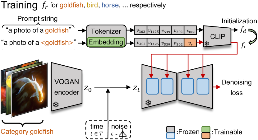
Figure 3: Training pipeline of GenPromp. The discriminative embedding $f_{d}$ is queried from a CLIP model while the representative embedding $f_{c}$ is learned through optimizing an image denoising model.

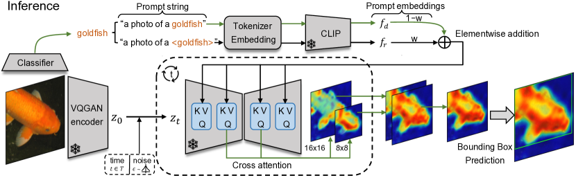
Figure 4: Inference pipeline of GenPromp. By performing a conditional denoising procedure, GenPromp produces object activation maps at multiple levels and timesteps. Two prompts (“a photo of a goldfish” and “a photo of a $\langle$goldfish$\rangle$”) are encoded to discriminative embedding $f_{d}$ and representative embedding $f_{r}$, which are combined to $f_{c}$. $f_{c}$ performs cross-attention with the features of the encoder and decoder in the image denoising model to obtain attention maps.

Learning Representative Embedding. Using solely the discriminative embedding $f_{d}$, GenPromp could miss representative yet less discriminative features. As an example in the second column and second row of Fig. 2, the activation map of the tower obtained by prompting the network with $f_{d}$ suffers from partial object activation. The representative embedding $f_{r}$ is thereby introduced as a prompt learning procedure, as shown in Fig. 3. In specific, the dictionary of the Tokenizer is extended by involving a new token ($i.e.$, $\langle{\rm\texttt{goldfish}}\rangle$), which is referred to as the concept token. The prompt with the concept token is encoded to the representative embedding $f_{r}$ through the pre-trained CLIP model.

Before learning, the representative embedding $f_{r}$ is initialized as the discriminative embedding $f_{d}$. When learning representative embedding, images belonging to a same category are collected to form the training set. Each input image is encoded to the latent variable $z_{0}$ by the VQGAN encoder, Fig. 3. Different levels of noises are added to $z_{0}$ to have a noisy latent $z_{t}$ through Eq. 2. The noisy latent $z_{t}$ is fed to the attention-unet $\epsilon_{\theta}$ to produce multi-layer feature maps $F_{l,t}$, where $l\in L$ index the encoded features of different layers. The Tokenizer Embedding layer in Fig. 3 incorporate embeddings for each word/token, where the embeddings ($i.e.$, $v_{r}$) of the corresponding concept tokens ($e.g.$, $\langle{\rm\texttt{goldfish}}\rangle$) are trainable. By optimizing a denoising procedure defined by stable diffusion, the representative embedding $f_{r}$ is learned, as

$$f_{r}^{*} =\mathop{\text{argmin}}\limits_{f_{r}}\mathcal{L}(\theta,f_{r}).$$ (4)

Benefiting from the property of the generative denoising model, $f_{r}^{*}$ can identify the common features among objects in the training set, learning representative features that define each category. As shown in the second column of Fig. 2, the activation map of tower obtained by prompting the network with $f_{r}$ activates the full object area.

Model Finetuning. After obtaining the representative embeddings $f_{r}^{*}$ for all image categories, the backbone network (attention-unet parameterized by $\epsilon_{\theta}$) is finetuned on the WSOL dataset, as

$$\theta^{*} =\mathop{\text{argmin}}\limits_{\theta}\mathcal{L}(\theta,f_{d})+\mathcal{L}(\theta,f_{r}^{*}),$$ (5)

which further optimizes the diffusion model using both $f_{d}$ and $f_{r}^{*}$ as prompts to reduce the domain gap between the model and the target dataset.

Combining Embeddings. After model finetuning, the discriminative and representative embeddings ($f_{d}$ and $f_{r}$) are linearly combined, as

$$f_{c} =w\cdot f_{r}+(1-w)\cdot f_{d},$$ (6)

where $w\in[0,1]$ is an experimentally determined weighted factor. As shown in Fig 2, for the category towel, a large $w$ activates background noise. Meanwhile, a small $w$ could cause partial object activation. An appropriate $w$ can balance the discriminative features and representative features of the categories, achieving the best localization performance.

5 Weakly Supervised Object Localization

As shown in Fig. 4, WSOL is defined as a conditional image denoising procedure. Similar to the training procedure, each input image is encoded to the latent variable $z_{0}$ by the VQGAN encoder. Different levels of noise are added to $z_{0}$ to generate noisy latent $z_{t}$ through Eq. 2. The noisy latent $z_{t}$ is fed to the finetuned attention-unet $\epsilon_{\theta^{*}}$ to produce multi-layer feature maps $F_{l,t}$, where $l\in L$ index the encoded features of different layers. Meanwhile, the input image is classified with a classifier pre-trained on the target dataset to obtain the category label, which is used to initialize two prompts (e.g.goldfish and $\langle\texttt{goldfish}\rangle$). According to Eq. 3, the two prompts are encoded to discriminative embedding $f_{d}$ and representative embedding $f_{r}$. The two embeddings are then combined to $f_{c}$, which is the condition for the image denoising model. Through performing denoising, cross attention maps are generated by using $F_{l,t}$ as the Query vector and $f_{c}$ as the Key vector, as

$$m_{l,t} =\text{CrossAttn}(F_{l,t},f_{c}),l\in L,t\in T.$$ (7)

One notable capability of GenPromp is to generate attention maps $\{m_{l,t}\}_{l\in L,t\in T}$ which exhibit distinct characteristics based on the specific layer $l$ at time $t$, as shown in Fig. 5. The characteristics of these attention maps can be concluded as follows: (1) Attention maps with higher resolution can provide more detailed localization clues but introduce more noise. (2) Attention maps of different layers can focus on different parts of the target object. (3) Smaller $t$ provides a less noisy background but tends to partial object activation. (4) Larger $t$ activates the target object more completely but introduces more background noise. Based on these observations, we propose to aggregate attention maps at multiple layers and timesteps to obtain a unified activation map, as

$$M =\frac{1}{|L|\cdot|T|}\sum_{l\in L,t\in T}\frac{m_{l,t}}{\text{max}(m_{l,t})}.$$ (8)

Experimentally, we find that aggregating the attention maps of spatial resolutions $8\times 8$ and $16\times 16$ at time steps $1$ and $100$ produces the best localization performance. A thresholding approach [73] is then applied to predict the object locations based on the unified activation map.

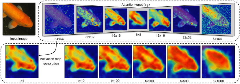
Figure 5: Aggregation of cross attention maps. Attention maps with respect to multiple resolutions and multiple noise levels (timesteps $t$) are aggregated to obtain the final localization map.

Method	Loc Back.	Cls Back.	CUB-200-2011			ImageNet-1K
			Top-1 Loc	Top-5 Loc	GT-known Loc	Top-1 Loc	Top-5 Loc	GT-known Loc
CAM${}_{\text{CVPR'16}}$ [75]	VGG16		41.1	50.7	55.1	42.8	54.9	59.0
TS-CAM${}_{\text{ICCV'21}}$ [22]	Deit-S		71.3	83.8	87.7	53.4	64.3	67.6
LCTR${}_{\text{AAAI'22}}$ [11]	Deit-S		79.2	89.9	92.4	56.1	65.8	68.7
SCM${}_{\text{ECCV'22}}$ [4]	Deit-S		76.4	91.6	96.6	56.1	66.4	68.8
CREAM${}_{\text{CVPR'22}}$ [65]	InceptionV3		71.8	86.4	90.4	56.1	66.2	69.0
BAS${}_{\text{CVPR'22}}$ [60]	ResNet50		77.3	90.1	95.1	57.2	67.4	71.8
PSOL${}_{\text{CVPR'20}}$ [69]	DenseNet161	EfficientNet-B7	80.9	90.0	91.8	58.0	65.0	66.3
C2AM${}_{\text{CVPR'22}}$ [63]	DenseNet161	EfficientNet-B7	81.8	91.1	92.9	59.6	67.1	68.5
GenPromp (Ours)	Stable Diffusion	EfficientNet-B7	87.0	96.1	98.0	65.1	73.3	74.9
GenPromp$\dagger$ (Ours)	Stable Diffusion	EfficientNet-B7	87.0	96.1	98.0	65.2	73.4	75.0

Table 1: Performance comparison of the proposed GenPromp approach with the state-of-the-art methods on the CUB-200-2011 test set and ImageNet-1K validation set. Loc Back. denotes the localization backbone, Cls Back. the backbone for classification, and $\dagger$ the prompt ensemble strategy, which ensembles the localization results from multiple prompts. Please refer to the supplementary for more comparison details.

6 Experiments

6.1 Experimental Settings

Datasets. We evaluate GenPromp on two commonly used benchmarks, $i.e.$, CUB-200-2011 and ImageNet-1K. CUB-200-2011 is a fine-grained bird dataset that contains 200 categories of birds with 5994 training images and 5794 test images. ImageNet-1K is a large-scale visual recognition dataset containing 1,000 categories with 1.2 million training images and 50,000 validation images.

Evaluation Metrics. We follow the previous methods and use Top-1 localization accuracy (Top-1 Loc), Top-5 localization accuracy (Top-5 Loc), and GT-known localization accuracy (GT-known Loc) as the metrics. For localization, a bounding box prediction is positive when it satisfies: (1) the predicted category label is correct, and (2) the IoU between the bounding box prediction and one of the ground-truth boxes is greater than 50$\%$. GT-known indicates that it considers only the IoU constraint regardless of the classification result.

Implementation Details. GenPromp is implemented based the Stable Diffusion model [50], which is pre-trained on LAION-5B [53]. The text encoder, $i.e.$, CLIP, is pre-trained on WIT [47]. During training, we resize the input image to 512$\times$512 and augment the training data with RandomHorizontalFlip and ColorJitter. We then optimize the network using AdamW with $\epsilon$=1$e$$-$8, $\beta_{1}$=0.9, $\beta_{2}$=0.999 and weight decay of 1$e$$-$2 on 8 RTX3090. In the training stage, we optimize GenPromp for 2 epochs with learning rate 5$e$$-$5 and batch size 8 for each category in CUB-200-2011 and ImageNet-1K. In the finetuning stage, we train GenPromp for 100,000 iterations with learning rate 5$e$$-$8 and batch size 128.

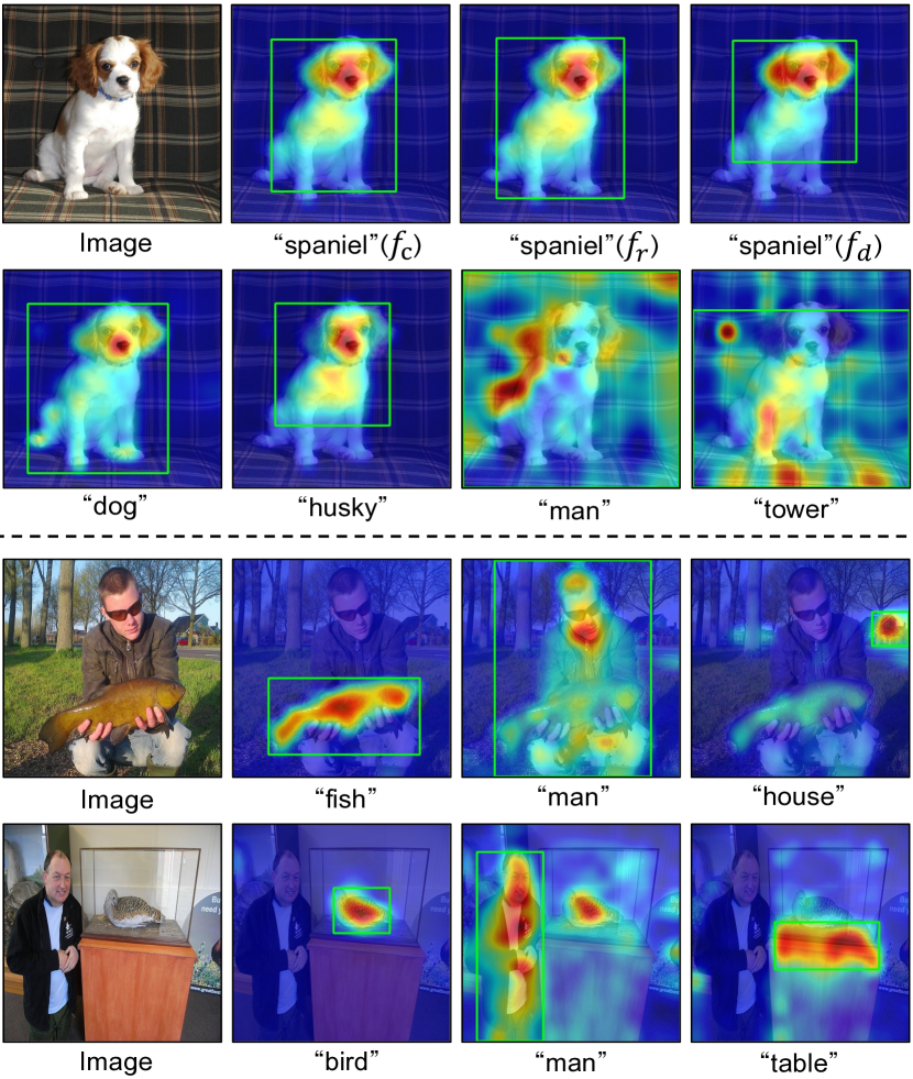
Figure 6: Object localization results of GenPromp using different prompt words. Words belonging to the same superclass activate the same object (upper), and words from different superclasses tend to activate different regions (upper and lower).

6.2 Main Results

Performance Comparison with SOTA Methods. In Table 1, the performance of the proposed GenPromp is compared with the state-of-the-art (SOTA) models. On CUB-200-2011 dataset, GenPromp achieves localization accuracy of Top-1 87.0%, Top-5 96.1%, which surpasses the SOTA methods by significant margins. Specifically, GenPromp achieves surprisingly 98.0% localization accuracy under GT-known metric, which shows the effectiveness of introducing generative model for WSOL. GenPromp outperforms the SOTA method $\text{C}^{2}\text{AM}$ [63] by 5.2% (87.0% $vs.$ 81.8%) and 5.0% (96.1% $vs.$ 91.1%) under Top-1 Loc and Top-5 Loc metrics respectively. When solely considering the localization performance (using GT-known Loc metric), GenPromp significantly outperforms the SOTA method SCM [4] by 1.4% (98.0% $vs.$ 96.6%). On the more challenging ImageNet-1K dataset, GenPromp also significantly outperforms the SOTA method $\text{C}^{2}\text{AM}$ [63] and BAS [60] by 5.6% (65.2% $vs.$ 59.6%), 6.0% (73.4% $vs.$ 67.4%), and 3.2% (75.0% $vs.$ 71.8%) under Top-1 Loc, Top-5 Loc and GT-known Loc metrics respectively. Such strong results clearly demonstrate the superiority of the generative model over conventional discriminative models for weakly supervised object localization.

Localization Results with respect to Prompt Embeddings. The localization results of GenPromp are shown in Fig. 6. In the first row of Fig. 6(upper), for the image with category spaniel, the discriminative prompt embedding $f_{d}$ fails to activate the legs, while the representative prompt embedding $f_{r}$ activates full object extent but suffering from the background noise. By combining $f_{d}$ and $f_{r}$, $f_{c}$ fully activates the object regions while maintaining low background noise. In the second row of Fig. 6(upper), we show the localization maps with prompt embeddings generated by different categories. Interestingly, categories that are highly related to spaniel ($i.e.,$ dog, husky) can also correctly activate the foreground object, which indicates that GenPromp is robust to the classifiers. When using the categories that are less related to spaniel ($i.e.$, man, tower) will introduce too much background noise and fail to localize the objects.

As shown in Fig. 6(lower), for the test images which contain multiple objects from various classes, GenPromp is able to generate high quality localization maps when given the corresponding prompt embeddings (generated using corresponding categories). The result demonstrates GenPromp can not only generate representative localization maps but also be able to discriminate object categories, revealing the potential of extending GenPromp to more challenging weakly supervised object detection or segmentation task.

Statistical Result with respect to Token Embeddings. In Fig. 7, the embedding vectors of the meta token are uniformly distributed in the two-dimensional feature space (yellow dots). After learning the representative embeddings/features of the categories, the embedding vectors of the concept token become uneven (blue dots), $i.e.$ less discriminative indicated by less deviation $\sigma_{x}$ and $\sigma_{y}$, which reveals the inconsistency between representative and discriminative embeddings.

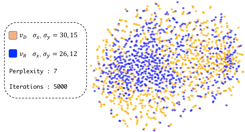
Figure 7: Statistical result of the embedding vectors of the meta token and the concept token for ImageNet-1K categories using tSNE. $\sigma_{x},\sigma_{y}$ respectively denote the standard deviation of the points in the $x$ and $y$ directions.

	Finetune	Embedding	ImageNet-1K
			Top-1 Loc	Top-5 Loc	GT-kno. Loc
1		$f_{d}$	61.2	69.0	70.4
2		$f_{r}$(w/o init)	44.6	50.2	51.3
3		$f_{r}$	64.0	72.1	73.7
4		$f_{c}$(w/o init)	56.2	63.2	64.5
5		$f_{c}$	64.5	72.7	74.2
6	✓	$f_{d}$	62.0	69.8	71.4
7	✓	$f_{r}$	64.9	73.1	74.6
8	✓	$f_{c}$	65.1	73.3	74.9

Table 2: Ablation studies of GenPromp.

6.3 Ablation Study

Baseline. We build the baseline method by using solely the discriminative embedding $f_{d}$ (Line 1 of Table 2). The performance (61.2% Top-1 Loc Acc.) of the baseline outperforms the SOTA methods, which indicates the great advantage of introducing the generative model for WSOL.

Representative Embedding. When using the trained representative embedding $f_{r}$ initialized by $f_{d}$ (Line 3 of Table 2), GenPromp outperforms the baseline by 2.8% (64.0% $vs.$ 61.2%) under Top-1 Loc metric, which validates the importance of the representative features of categories for object localization. We also train representative embedding $f_{r}$ which is random initialized (Line 2 of Table 2). The performance of $f_{r}$ drops to very low-level suffering from the local optimal embeddings.

Method	Loc Back.	Cls Back.	Params.	ImageNet-1K
				Top-1 Loc	Top-5 Loc	GT-known Loc	Top-1 Cls	Top-5 Cls
TS-CAM [22]	Deit-S (ImageNet-1K)		22.4M	53.4	64.3	67.6	74.3	92.1
TS-CAM [22]	ViT-H (LAION-2B [53], ImageNet-1K)		633M	42.1	49.9	52.2	77.4	93.7
GenPromp$\dagger$	Stable Diffusion	EfficientNet-B7	1017M + 66M	65.2	73.4	75.0	85.1	97.2

Table 3: Performance comparison with respect to model size and training data. With a larger backbone and pre-training dataset, the discriminatively trained method TS-CAM does not achieve higher performance.

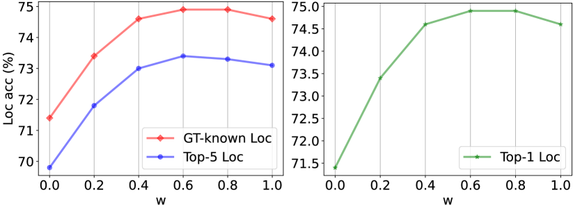
Figure 8: Localization accuracy under IoUs on ImageNet-1K using different embedding combination weights $w$.

Embedding Combination. By combining $f_{r}$ and $f_{d}$, the performance of GenPromp can be further boost to 64.5% in Top-1 Loc (Line 5 of Table 2). We also conduct experiments to show the effect of the combination weight $w$ on ImageNet 1K dataset. The performance keeps consistent when the combination weight $w$ falls to $[0.4,0.8]$, as shown in Fig. 8. With a proper $w$, GenPromp is able to generate discriminative while representative prompt embeddings and active full object extent with the least background noise.

Model Finetuning. By filling the domain gap through finetuning the backbone network (attention-unet), a performance gain of $0.6\%$ (65.1% $vs.$ 64.5%) can be achieved in Top-1 Loc (Line 8 of Table 2).

Timesteps	ImageNet-1K
	Top-1 Loc	Top-5 Loc	GT-known Loc
1	64.6	72.7	74.3
10	64.8	72.9	74.5
100	64.9	73.1	74.6
200	64.6	72.7	74.3
500	59.4	66.9	68.3
1000	42.8	48.3	49.3
1+100	65.1	73.3	74.9
1+100+200	65.1	73.3	74.9
1+100+200+500	64.1	72.2	73.7

Table 4: Performance under test timesteps.

Model Size and Training Data. In Table 3, we re-implement TS-CAM with larger backbone (e.g.ViT-H) and more training data (e.g.LAION-2B). The re-implemented TS-CAM achieves higher classification accuracy while much lower localization accuracy compared to the Deit-S based TS-CAM. We attribute this to the inherent flaw of the discriminatively trained classification model, $i.e.$, local discriminative regions are capable of minimizing image classification loss, but experience difficulty in accurate object localization. A larger backbone and more training data even make this phenomenon even more serious.

Resolution	ImageNet-1K
	Top-1 Loc	Top-5 Loc	GT-known Loc
8	58.5	65.7	67.1
16	62.5	70.5	72.0
32	38.0	42.7	43.6
64	17.5	19.9	20.3
8+16	65.1	73.3	74.9
8+16+32	64.2	72.2	73.7

Table 5: Performance under attention map resolutions.

Effect of Timesteps and Resolutions. In Tables 4 and  5, we evaluate the performance by aggregating attention maps under different timesteps and spatial resolutions. It can be seen that aggregating the attention maps of spatial resolutions $8\times 8$ and $16\times 16$ at time steps $1$, $100$ produces the best localization performance.

7 Conclusion and Future Remark

To solve the partial object activation brought by discriminatively trained activation models in a systematic way, we propose GenPromp, which formulates WSOL as a conditional image denoising procedure. During training, we use the learnable embeddings to conditionally recover the input image with the aim to learn the representative embeddings. During inference, GenPromp first combines the trained representative embeddings with another discriminative embeddings from the pre-trained CLIP model. The combined embeddings are then used to generate attention maps at multiple timesteps and resolutions, which facilitate localizing the full object extent. GenPromp not only sets a solid baseline for WSOL with generative models but also provides fresh insight for handling vision tasks using vision-language models.

When claiming the advantages of GenPromp, we also realize its disadvantages. One major disadvantage is its dependency on large-scale pre-trained vision-language models, which could slow down the inference speed and raise the requirement for GPU memory cost. Such a disadvantage should be solved in future work.

Dataset	Ann.	# Images	How to collect	$t$ (s/img)
CUB-200-2011 [56]	$\mathcal{I}$	11,788	Manual	1.5
Imagenet [52]	$\mathcal{I}$	14,197,122	Manual	1.5
JFT-3B [19]	$\mathcal{I}^{\dagger}$	3,000,000,000	Semi-automatic	$\approx 0$
CC12M [7]	$\mathcal{T}^{\dagger}$	12,000,000	Web crawler	$\approx 0$
WIT [47]	$\mathcal{T}^{\dagger}$	400,000,000	Web crawler	$\approx 0$
LAION-400M [54]	$\mathcal{T}^{\dagger}$	400,000,000	Web crawler	$\approx 0$
LAION-5B [53]	$\mathcal{T}^{\dagger}$	5,850,000,000	Web crawler	$\approx 0$
Cityscapes [15]	$\mathcal{B}$	25,000	Manual	37.5
COCO [37]	$\mathcal{B}$	328,000	Manual	37.5

Table 6: The size and data collecting approaches of some commonly used datasets. $\mathcal{I},\mathcal{T},\mathcal{B}$ denotes the image category labels, text descriptions and bounding box annotations respectively. $t$ denotes the average annotation time per image. $\dagger$ indicates the annotation is noisy.

Appendix A Annotation Cost

As shown in Table 6, we compare the size and data collection methods of commonly used datasets with three types of annotations: image category labels, text descriptions, and bounding boxes. It can be observed that datasets with accurate bounding box labels, such as Cityscapes and COCO, are usually small in size due to the high cost of manual annotation. However, when using image category labels, the dataset size can be increased to 14 million (e.g., ImageNet). For datasets with a huge size, such as JFT-3B, WIT, and LAION-5B, manual annotation becomes impractical. Instead, semi-automatic annotation methods or web crawler algorithms are used to extensively collect noisy annotated data. Thanks to the rapid development of the Internet, a large number of image-text pairs can be found in websites, forums, and libraries, which are naturally annotated by citizens and can be easily obtained by crawler algorithms. Since collecting image-text pairs hardly requires human participation, their annotation cost is negligible. In this paper, the proposed method GenPromp is implemented based the Stable Diffusion model, which is pre-trained on LAION-5B. Accordingly, GenPromp hardly introduces additional annotation cost for a weakly supervised learning system.

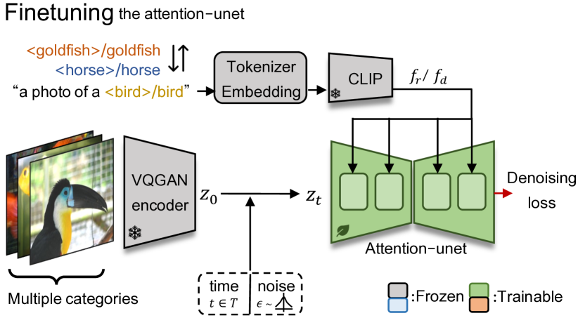
Figure 9: Finetuning pipeline of GenPromp.

Appendix B Finetuning

As described in Section 4 in the main document, after obtaining the representative embeddings $f_{r}^{*}$ for all image categories, we finetune the attention-unet (parameterized by $\epsilon_{\theta}$) to reduce the domain gap between the model and the target dataset. We demonstrate the pipeline of finetuning in Fig. 9. The finetuning pipeline is different from the training pipeline (shown in Fig. 3 of the main document) in two aspects: (1) Each training batch contains images of multiple categories, (2) The prompt embeddings are frozen while the attention-unet is trainable.

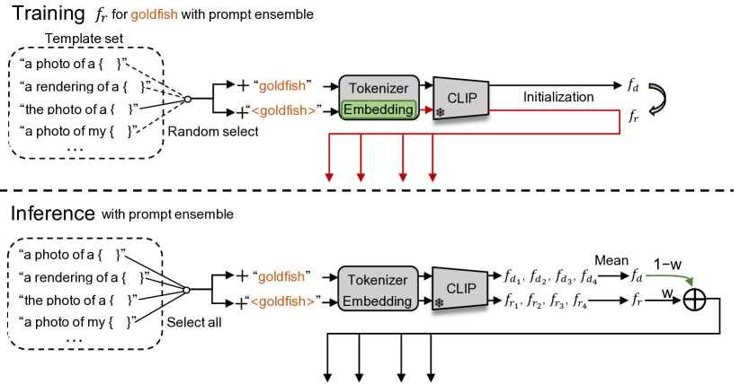
Figure 10: Workflow of the proposed prompt ensemble strategy. The image encoding and activate map generation procedure are omitted for clarity.

Appendix C Prompt Ensemble

To further improve the performance of GenPromp, we propose a prompt ensemble strategy. As shown in Fig. 10, during training, we random select a template from a template set. Then, we respectively fill the meta token (goldfish) and the concept token ($\langle\texttt{goldfish}\rangle$) into the template to obtain the two input prompts, which are used to learn the representative embedding $f_{r}$. During inference, for each template in the template set, we combines it with the two tokens to form the input prompts. Then, all the prompts are encoded into prompt embeddings by the pre-trained CLIP model. After that, the discriminative embedding $f_{d}$ is obtained by averaging the discriminative embeddings generated by different templates (e.g.$f_{d_{1}},f_{d_{2}},f_{d_{3}},f_{d_{4}}$ in Fig. 10), the representative embedding $f_{r}$ is obtained by averaging the representative embeddings generated by different templates (e.g.$f_{r_{1}},f_{r_{2}},f_{r_{3}},f_{r_{4}}$ in Fig. 10). Finally, $f_{d}$ and $f_{r}$ are combined to $f_{c}$, which is fed into the network to generate attention maps. In experiments, we use a template set that consists of 7 templates:

“a photo of a { }”

“a rendering of a { }”

“the photo of a { }”

“a photo of my { }”

“a photo of the { }”

“a photo of one { }”

“a rendition of a { }”

Embedding	ImageNet-1K
	Top-1 Loc	Top-5 Loc	GT-known Loc	M-Ins	Part	More
$f_{d}$	62.2	70.0	71.5	9.4	3.8	8.2
$f_{r}$	64.9	73.1	74.7	9.5	2.4	7.3
$f_{c}$	65.2	73.4	75.0	9.1	3.0	6.9

Table 7: Localization error statistics. The results are correspond to row 17-19 in Table 11. “M-Ins”, “Part” and “More” denote the multi-instance error, localization part error and localization more error respectively.

Noise $\epsilon$	ImageNet-1K
	Top-1 Loc	Top-5 Loc	GT-known Loc
	64.8	73.0	74.6
✓	65.1	73.3	74.9

Table 8: Evaluation of noise levels in the inference time. For the experiment that includes noise $\epsilon$ in the inference time, we conduct 10 experiments under different random seeds and average their results as the final result.

Method	Loc Back.	Cls Back.	CUB-200-2011			ImageNet-1K
			Top-1 Loc	Top-5 Loc	GT-known Loc	Top-1 Loc	Top-5 Loc	GT-known Loc
CAM${}_{\text{CVPR'16}}$ [75]	VGG16		41.1	50.7	55.1	42.8	54.9	59.0
ADL${}_{\text{CVPR'19}}$ [13]	VGG16		52.4	-	75.4	44.9	-	-
DANet${}_{\text{ICCV'19}}$ [67]	VGG16		52.5	62.0	67.7	-	-	-
SLT${}_{\text{CVPR'21}}$ [27]	VGG16		67.8	-	87.6	51.2	62.4	67.2
FAM${}_{\text{ICCV'21}}$ [41]	VGG16		69.3	-	89.3	52.0	-	71.7
TAFormer${}_{\text{TPAMI'22}}$ [42]	VGG16		72.0	85.9	90.8	53.4	67.7	74.0
BAS${}_{\text{CVPR'22}}$ [60]	VGG16		71.3	85.3	91.1	53.0	65.4	69.6
CAM${}_{\text{CVPR'16}}$ [75]	MobileNetV1		48.1	59.2	63.3	43.4	54.4	59.0
HaS${}_{\text{ICCV'17}}$ [55]	MobileNetV1		46.7	-	67.3	42.7	-	60.1
ADL${}_{\text{CVPR'19}}$ [13]	MobileNetV1		47.7	-	-	43.0	-	-
FAM${}_{\text{ICCV'21}}$ [41]	MobileNetV1		65.7	-	85.7	46.2	-	62.1
TAFormer${}_{\text{TPAMI'22}}$ [42]	MobileNetV1		66.7	80.2	85.0	47.6	65.5	68.8
BAS${}_{\text{CVPR'22}}$ [60]	MobileNetV1		69.8	86.0	92.4	53.0	66.6	72.0
CAM${}_{\text{CVPR'16}}$ [75]	ResNet50		46.7	54.4	57.4	39.0	49.5	51.9
ADL${}_{\text{CVPR'19}}$ [13]	ResNet50-SE		62.3	-	-	-	-	48.5
FAM${}_{\text{ICCV'21}}$ [41]	ResNet50		73.7	-	85.7	54.5	-	64.6
SPOL${}_{\text{CVPR'21}}$ [59]	ResNet50		80.1	93.4	96.5	59.1	67.2	69.0
TAFormer${}_{\text{TPAMI'22}}$ [42]	ResNet50		75.0	87.8	91.2	57.5	69.9	75.5
DA${}_{\text{CVPR'22}}$ [76]	ResNet50		66.7	-	81.8	55.8	-	70.3
BAS${}_{\text{CVPR'22}}$ [60]	ResNet50		77.3	90.1	95.1	57.2	67.4	71.8
CAM${}_{\text{CVPR'16}}$ [75]	InceptionV3		41.1	50.7	55.1	46.3	58.2	62.7
DANet${}_{\text{ICCV'19}}$ [67]	InceptionV3		49.5	60.5	67.0	47.5	58.3	-
SLT${}_{\text{CVPR'21}}$ [27]	InceptionV3		66.1	-	86.5	55.7	65.4	67.6
FAM${}_{\text{ICCV'21}}$ [41]	InceptionV3		70.7	-	87.3	55.2	-	68.6
TAFormer${}_{\text{TPAMI'22}}$ [42]	InceptionV3		73.3	84.1	88.7	56.0	66.5	69.8
BAS${}_{\text{CVPR'22}}$ [60]	InceptionV3		73.3	86.3	92.2	58.5	69.0	71.9
CREAM${}_{\text{CVPR'22}}$ [65]	InceptionV3		71.8	86.4	90.4	56.1	66.2	69.0
TS-CAM${}_{\text{ICCV'21}}$ [22]	Deit-S		71.3	83.8	87.7	53.4	64.3	67.6
LCTR${}_{\text{AAAI'22}}$ [11]	Deit-S		79.2	89.9	92.4	56.1	65.8	68.7
SCM${}_{\text{ECCV'22}}$ [4]	Deit-S		76.4	91.6	96.6	56.1	66.4	68.8
DiPS${}_{\text{WACVW'23}}$ [45]	Deit-S	TransFG [28]	88.2	-	-	-	-	-
PSOL${}_{\text{CVPR'20}}$ [69]	DenseNet161	EfficientNet-B7	80.9	90.0	91.8	58.0	65.0	66.3
C2AM${}_{\text{CVPR'22}}$ [63]	DenseNet161	EfficientNet-B7	81.8	91.1	92.9	59.6	67.1	68.5
GenPromp (Ours)	Stable Diffusion	EfficientNet-B7	87.0	96.1	98.0	65.1	73.3	74.9
GenPromp$\dagger$ (Ours)	Stable Diffusion	EfficientNet-B7	87.0	96.1	98.0	65.2	73.4	75.0
GenPromp$\dagger$ (Ours)	Stable Diffusion	TransFG [28]	89.3	96.5	98.0	-	-	-

Table 9: Performance comparison of the proposed GenPromp approach with the state-of-the-art methods on the CUB-200-2011 test set and ImageNet-1K validation set. Loc Back. denotes the localization backbone, Cls Back. the backbone for classification, and $\dagger$ the prompt ensemble strategy, which ensembles the localization results from multiple prompts.

Appendix D Additional Experimental Results

Complete Performance Comparison with SOTA Methods. Table 9 shows the complete performance comparison of the proposed GenPromp and the state-of-the-art (SOTA) models (extension of Table 1 in the main document). On CUB-200-2011 and ImageNet-1K dataset, GenPromp surpasses the SOTA methods by significant margins. Such strong results clearly demonstrate the superiority of the generative model over conventional discriminative models for weakly supervised object localization.

Localization Error Analysis. To further reveal the effect of the proposed prompt embeddings (e.g.$f_{d}$, $f_{r}$, $f_{c}$), following TS-CAM [22], we evaluate the localization errors of: multi-instance error (M-Ins), localization part error (Part), and localization more error (More). They are respectively defined as follows.

• M-Ins indicates that the predicted bounding box intersects with at least two ground-truth boxes, and $\text{IoG}>0.3$.

• Part indicates that the predicted bounding box only cover the parts of object, and $\text{IoP}>0.5$.

• More indicates that the predicted bounding box is larger than the ground truth bounding box by a large margin, and $\text{IoG}>0.7$.

where IoG and IoP are defined as Intersection over Ground truth box and Intersection over Predict bounding box, respectively (similar to IoU (Intersection over Union)). Each metric calculates the percentage of images belonging to corresponding error in the validation/test set. Please refer to TS-CAM [22] for a detailed definition of the three metrics. Table 7 lists localization error statistics of M-Ins, Part, and More. Compare to the discriminative embedding $f_{d}$, the learned representative embedding $f_{r}$ reduces both Part and More errors by 1.4% (3.8% $vs.$ 2.4%) and 0.9% (8.2% $vs.$ 7.3%) respectively, demonstrating that the representative embedding alleviates the partial object activation problem. By combining the representative embedding $f_{r}$ with the discriminative embedding $f_{d}$, the More errors drop 0.4% (7.3% $vs.$ 6.9%) while the Part errors increase 0.6% (3.0% $vs.$ 2.4%) compared to $f_{r}$. This demonstrates that $f_{c}$ can further depress the background noise while keeping relatively low Part errors.

Effect of Noise $\epsilon$. In Table 8, we evaluate the performance by setting the noise $\epsilon$ (in Eq. 1 and Eq. 2 of the main document) to 0 during inference. Without noise $\epsilon$, the performance of GenPromp drops 0.3% in Top-1 Loc in average. Similar to the methods [13, 14, 39, 55, 68, 73] based on adversarial erasing, the input noise in GenPromp can also alleviate the part activation issue, which drives the network to mine the representative yet less discriminative object parts.

Method	Loc Back.	Cls Back.	Params.	CUB-200-2011
				Top-1 Loc	Top-5 Loc	GT-known Loc	Top-1 Cls	Top-5 Cls
TS-CAM [22]	Deit-S (ImageNet-1K)		22.4M	71.3	83.8	87.7	80.3	94.8
TS-CAM [22]	Deit-B (ImageNet-1K)		87.2M	75.8	84.1	86.6	86.8	96.7
TS-CAM [22]	ViT-L (LAION-2B [53], ImageNet-1K, CUB(60epochs ft))		304M	63.4	76.0	80.1	77.3	93.8
TS-CAM [22]	ViT-H (LAION-2B [53], ImageNet-1K, CUB(60epochs ft))		633M	10.7	20.2	32.9	29.1	56.8
GenPromp$\dagger$	Stable Diffusion	EfficientNet-B7	1017M + 66M	87.0	96.1	98.0	88.7	97.9

Method	Loc Back.	Cls Back.	Params.	ImageNet-1K
				Top-1 Loc	Top-5 Loc	GT-known Loc	Top-1 Cls	Top-5 Cls
TS-CAM [22]	Deit-S (ImageNet-1K)		22.4M	53.4	64.3	67.6	74.3	92.1
TS-CAM [22]	ViT-H (LAION-2B [53], ImageNet-1K(3epochs ft))		633M	41.9	50.7	53.2	74.7	92.8
TS-CAM [22]	ViT-H (LAION-2B [53], ImageNet-1K(6epochs ft))		633M	42.1	49.9	52.2	77.4	93.7
GenPromp$\dagger$	Stable Diffusion	EfficientNet-B7	1017M + 66M	65.2	73.4	75.0	85.1	97.2

Table 10: Performance comparison with respect to model size and training data. With a larger backbone and pre-training dataset, the discriminatively trained method TS-CAM does not achieve higher performance.

	Multi-resolution	Multi-timesteps	Prompt Ensemble	Prompt Embedding	Finetune	ImageNet-1K
						Top-1 Loc	Top-5 Loc	GT-known Loc
1				$f_{d}$		58.5	66.0	67.4
2	✓			$f_{d}$		58.6	66.1	67.5
3		✓		$f_{d}$		58.6	66.0	67.5
4	✓	✓		$f_{d}$		61.2	69.0	70.4
5	✓	✓		$f_{r}$ (w/o init)		44.6	50.2	51.3
6	✓	✓		$f_{r}$		64.0	72.1	73.7
7	✓	✓		$f_{c}$ (w/o init)		56.2	63.2	64.5
8	✓	✓		$f_{c}$		64.5	72.7	74.2
9	✓	✓	✓	$f_{d}$		61.5	69.2	70.7
10	✓	✓	✓	$f_{r}$		64.2	72.3	73.8
11	✓	✓	✓	$f_{c}$		64.6	72.8	74.3
12	✓	✓		$f_{d}$	✓	62.0	69.8	71.4
13	✓	✓		$f_{r}$	✓	64.9	73.1	74.6
14	✓	✓		$f_{c}$	✓	65.1	73.3	74.9
15	✓		✓	$f_{c}$	✓	65.0	73.2	74.8
16		✓	✓	$f_{c}$	✓	62.3	70.3	71.8
17	✓	✓	✓	$f_{d}$	✓	62.2	70.0	71.5
18	✓	✓	✓	$f_{r}$	✓	64.9	73.1	74.7
19	✓	✓	✓	$f_{c}$	✓	65.2	73.4	75.0

Table 11: Ablation of main components of GenPromp. For experiments that do not have a “$\checkmark$” in Multi-resolution or Multi-timesteps, we use a single resolution (16$\times$ 16) or a single timestep ($t=100$) for model inference.

Additional Restults with respect to Model Size and Training Data. In Table 10, we re-implement TS-CAM with larger backbone (e.g.Deit-B, ViT-L, ViT-H) and more training data (e.g.LAION-2B). As the model size getting larger, the performance of TS-CAM becomes worse on CUB-200-2011 under GT-known Loc metric, Table 10(upper). As shown in Table 10(lower), by finetuning ViT-H-based TS-CAM for 3 epochs on ImageNet-1K, it achieves higher classification accuracy (74.7% $vs.$ 74.3% on Top-1 Cls) while much lower localization accuracy (53.2% $vs.$ 67.6% on GT-known Loc) compared to the Deit-S-based TS-CAM. By finetuning the model for more epochs (e.g.6 epochs), it achievea higher classification accuracy (77.4% $vs.$ 74.7% on Top-1 Cls) but lower localization accuracy (52.2% $vs.$ 53.2% under GT-known Loc metric), demonstrating that more epochs can not improve the localization performance of TS-CAM. We attribute this phenomenon to the inherent flaw of the discriminatively trained classification model, $i.e.$, local discriminative regions are capable of minimizing image classification loss but experience difficulty in accurate object localization. A larger backbone and more training data make this phenomenon even more serious.

Detailed Ablation Study. Table 11 provides a detailed ablation of the performance contribution of each component and their combinations, with respect to Multi-resolution, Multi-timesteps, Prompt ensemble, Prompt embedding and Finetuning.

Appendix E Additional Visualization Results

In Fig. 11, we visualize the localization results of GenPromp and compared them with the discriminatively trained model (e.g.CAM [75]). The object Localization maps of CAM (column b) suffer from partial object activation. Localization maps of GenPromp (column d) with sole representative embeddings ($f_{r}$) covers more object extent but introducing background noise. Those of GenPromp (column e) with combined embeddings ($f_{c}$) not only activate full object extent but also depress background noise for precise object localization.

We also provide additional visualization results of Fig. 2, Fig. 5 and Fig. 6 in the main document. The results are shown in Fig. 12, Fig. 13 and Fig. 14 respectively.

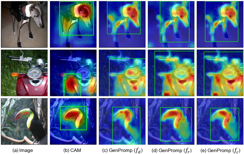
Figure 11: Comparison of activation maps between CAM and GenPromp.

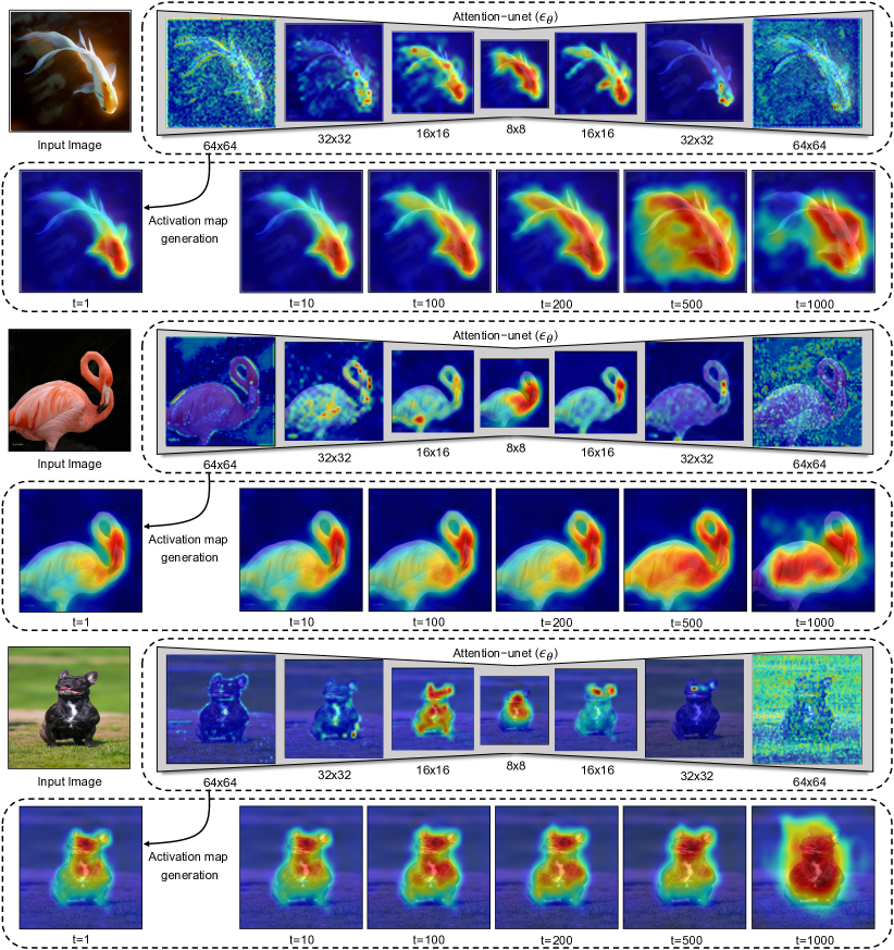
Figure 12: Visualization of cross attention maps. Attention maps with respect to multiple resolutions and multiple noise levels (timesteps $t$) are aggregated to obtain the final localization map. The characteristics of these attention maps can be concluded as follows: (1) Attention maps with higher resolution can provide more detailed localization clues but introduce more noise. (2) Attention maps of different layers can focus on different parts of the target object. (3) Smaller $t$ provides a less noisy background but tends to partial object activation. (4) Larger $t$ activates the target object more completely but introduces more background noise.

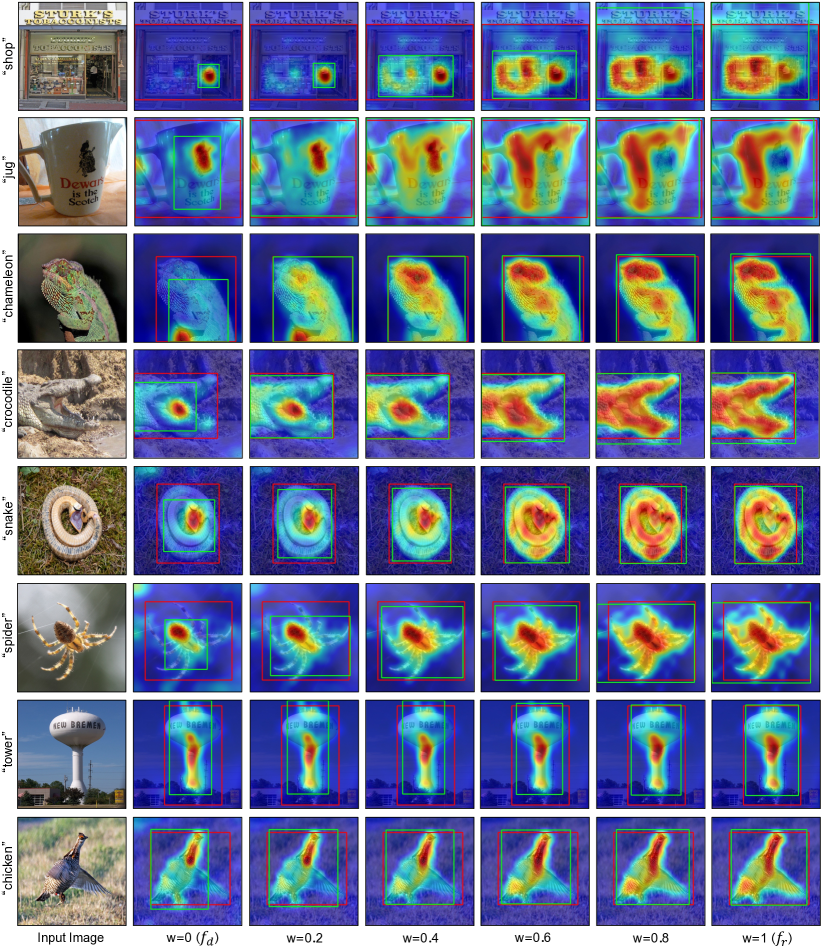
Figure 13: Activation maps and localization results using discriminative and representative embeddings. A proper combination of discriminative embeddings $f_{d}$ with representative embedding $f_{r}$ as the prompt produces precise activation maps and good WSOL results (green boxes).

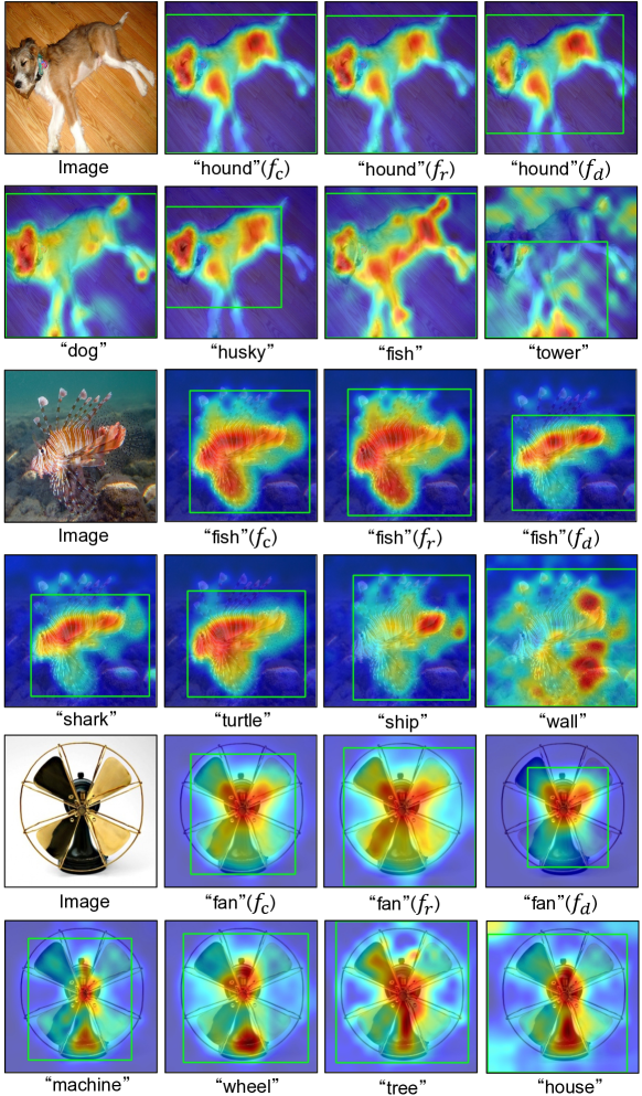
Figure 14: Object localization results of GenPromp using different prompt words.

References

- [1] Tomer Amit, Eliya Nachmani, Tal Shaharabany, and Lior Wolf. Segdiff: Image segmentation with diffusion probabilistic models. CoRR, abs/2112.00390, 2021.
- [2] Martín Arjovsky, Soumith Chintala, and Léon Bottou. Wasserstein GAN. CoRR, abs/1701.07875, 2017.
- [3] Wonho Bae, Junhyug Noh, and Gunhee Kim. Rethinking class activation mapping for weakly supervised object localization. In Andrea Vedaldi, Horst Bischof, Thomas Brox, and Jan-Michael Frahm, editors, ECCV, pages 618–634, 2020.
- [4] Haotian Bai, Ruimao Zhang, Jiong Wang, and Xiang Wan. Weakly supervised object localization via transformer with implicit spatial calibration. In ECCV, pages 612–628, 2022.
- [5] Dmitry Baranchuk, Andrey Voynov, Ivan Rubachev, Valentin Khrulkov, and Artem Babenko. Label-efficient semantic segmentation with diffusion models. In ICLR, 2022.
- [6] Andrew Brock, Jeff Donahue, and Karen Simonyan. Large scale GAN training for high fidelity natural image synthesis. In ICLR, 2019.
- [7] Soravit Changpinyo, Piyush Sharma, Nan Ding, and Radu Soricut. Conceptual 12m: Pushing web-scale image-text pre-training to recognize long-tail visual concepts. In IEEE CVPR, pages 3558–3568, 2021.
- [8] David L. Chen and William B. Dolan. Collecting highly parallel data for paraphrase evaluation. In Dekang Lin, Yuji Matsumoto, and Rada Mihalcea, editors, ACL, pages 190–200, 2011.
- [9] Shoufa Chen, Peize Sun, Yibing Song, and Ping Luo. Diffusiondet: Diffusion model for object detection. CoRR, abs/2211.09788, 2022.
- [10] Zhang Chen, Zhiqiang Tian, Jihua Zhu, Ce Li, and Shaoyi Du. C-CAM: causal CAM for weakly supervised semantic segmentation on medical image. In IEEE CVPR, pages 11666–11675, 2022.
- [11] Zhiwei Chen, Changan Wang, Yabiao Wang, Guannan Jiang, Yunhang Shen, Ying Tai, Chengjie Wang, Wei Zhang, and Liujuan Cao. LCTR: on awakening the local continuity of transformer for weakly supervised object localization. In AAAI, pages 410–418, 2022.
- [12] Gong Cheng, Junyu Yang, Decheng Gao, Lei Guo, and Junwei Han. High-quality proposals for weakly supervised object detection. TIP, pages 5794–5804, 2020.
- [13] Junsuk Choe, Seungho Lee, and Hyunjung Shim. Attention-based dropout layer for weakly supervised single object localization and semantic segmentation. IEEE TPAMI, pages 4256–4271, 2021.
- [14] Junsuk Choe and Hyunjung Shim. Attention-based dropout layer for weakly supervised object localization. In IEEE CVPR, pages 2219–2228, 2019.
- [15] Marius Cordts, Mohamed Omran, Sebastian Ramos, Timo Rehfeld, Markus Enzweiler, Rodrigo Benenson, Uwe Franke, Stefan Roth, and Bernt Schiele. The cityscapes dataset for semantic urban scene understanding. In IEEE CVPR, pages 3213–3223, 2016.
- [16] Pradipto Das, Chenliang Xu, Richard F. Doell, and Jason J. Corso. A thousand frames in just a few words: Lingual description of videos through latent topics and sparse object stitching. In IEEE CVPR, pages 2634–2641, 2013.
- [17] Jacob Devlin, Ming-Wei Chang, Kenton Lee, and Kristina Toutanova. BERT: pre-training of deep bidirectional transformers for language understanding. In Jill Burstein, Christy Doran, and Thamar Solorio, editors, NAACL-HLT, pages 4171–4186, 2019.
- [18] Prafulla Dhariwal and Alexander Quinn Nichol. Diffusion models beat gans on image synthesis. In Marc’Aurelio Ranzato, Alina Beygelzimer, Yann N. Dauphin, Percy Liang, and Jennifer Wortman Vaughan, editors, NeurIPS, pages 8780–8794, 2021.
- [19] Alexey Dosovitskiy, Lucas Beyer, Alexander Kolesnikov, Dirk Weissenborn, Xiaohua Zhai, Thomas Unterthiner, Mostafa Dehghani, Matthias Minderer, Georg Heigold, Sylvain Gelly, Jakob Uszkoreit, and Neil Houlsby. An image is worth 16x16 words: Transformers for image recognition at scale. In ICLR, 2021.
- [20] Patrick Esser, Robin Rombach, and Björn Ommer. Taming transformers for high-resolution image synthesis. In IEEE CVPR, pages 12873–12883, 2021.
- [21] Rinon Gal, Yuval Alaluf, Yuval Atzmon, Or Patashnik, Amit H. Bermano, Gal Chechik, and Daniel Cohen-Or. An image is worth one word: Personalizing text-to-image generation using textual inversion. CoRR, abs/2208.01618, 2022.
- [22] Wei Gao, Fang Wan, Xingjia Pan, Zhiliang Peng, Qi Tian, Zhenjun Han, Bolei Zhou, and Qixiang Ye. TS-CAM: token semantic coupled attention map for weakly supervised object localization. In ICCV, pages 2866–2875, 2021.
- [23] Wei Gao, Fang Wan, Jun Yue, Songcen Xu, and Qixiang Ye. Discrepant multiple instance learning for weakly supervised object detection. PR, page 108233, 2022.
- [24] Chen Gong, Zhou Yang, Yunpeng Bai, Jieke Shi, Arunesh Sinha, Bowen Xu, David Lo, Xinwen Hou, and Guoliang Fan. Curiosity-driven and victim-aware adversarial policies. In Proceedings of the 38th Annual Computer Security Applications Conference, pages 186–200, 2022.
- [25] Ian J. Goodfellow, Jean Pouget-Abadie, Mehdi Mirza, Bing Xu, David Warde-Farley, Sherjil Ozair, Aaron C. Courville, and Yoshua Bengio. Generative adversarial networks. Commun. ACM, pages 139–144, 2020.
- [26] Ishaan Gulrajani, Faruk Ahmed, Martín Arjovsky, Vincent Dumoulin, and Aaron C. Courville. Improved training of wasserstein gans. In Isabelle Guyon, Ulrike von Luxburg, Samy Bengio, Hanna M. Wallach, Rob Fergus, S. V. N. Vishwanathan, and Roman Garnett, editors, NeurIPS, pages 5767–5777, 2017.
- [27] Guangyu Guo, Junwei Han, Fang Wan, and Dingwen Zhang. Strengthen learning tolerance for weakly supervised object localization. In IEEE CVPR, pages 7403–7412, 2021.
- [28] Ju He, Jie-Neng Chen, Shuai Liu, Adam Kortylewski, Cheng Yang, Yutong Bai, and Changhu Wang. Transfg: A transformer architecture for fine-grained recognition. In AAAI, pages 852–860, 2022.
- [29] Amir Hertz, Ron Mokady, Jay Tenenbaum, Kfir Aberman, Yael Pritch, and Daniel Cohen-Or. Prompt-to-prompt image editing with cross attention control. CoRR, abs/2208.01626, 2022.
- [30] Jonathan Ho, Ajay Jain, and Pieter Abbeel. Denoising diffusion probabilistic models. In Hugo Larochelle, Marc’Aurelio Ranzato, Raia Hadsell, Maria-Florina Balcan, and Hsuan-Tien Lin, editors, NeurIPS, 2020.
- [31] Phillip Isola, Jun-Yan Zhu, Tinghui Zhou, and Alexei A. Efros. Image-to-image translation with conditional adversarial networks. In IEEE CVPR, pages 5967–5976, 2017.
- [32] Tero Karras, Timo Aila, Samuli Laine, and Jaakko Lehtinen. Progressive growing of gans for improved quality, stability, and variation. In ICLR, 2018.
- [33] Tero Karras, Samuli Laine, and Timo Aila. A style-based generator architecture for generative adversarial networks. In IEEE CVPR, pages 4401–4410, 2019.
- [34] Tero Karras, Samuli Laine, and Timo Aila. A style-based generator architecture for generative adversarial networks. TPAMI, pages 4217–4228, 2021.
- [35] Bahjat Kawar, Shiran Zada, Oran Lang, Omer Tov, Huiwen Chang, Tali Dekel, Inbar Mosseri, and Michal Irani. Imagic: Text-based real image editing with diffusion models. CoRR, abs/2210.09276, 2022.
- [36] Eunji Kim, Siwon Kim, Jungbeom Lee, Hyunwoo Kim, and Sungroh Yoon. Bridging the gap between classification and localization for weakly supervised object localization. In IEEE CVPR, pages 14238–14247, 2022.
- [37] Tsung-Yi Lin, Michael Maire, Serge J. Belongie, James Hays, Pietro Perona, Deva Ramanan, Piotr Dollár, and C. Lawrence Zitnick. Microsoft COCO: common objects in context. In David J. Fleet, Tomás Pajdla, Bernt Schiele, and Tinne Tuytelaars, editors, ECCV, pages 740–755, 2014.
- [38] Weizeng Lu, Xi Jia, Weicheng Xie, Linlin Shen, Yicong Zhou, and Jinming Duan. Geometry constrained weakly supervised object localization. In Andrea Vedaldi, Horst Bischof, Thomas Brox, and Jan-Michael Frahm, editors, ECCV, pages 481–496, 2020.
- [39] Jinjie Mai, Meng Yang, and Wenfeng Luo. Erasing integrated learning: A simple yet effective approach for weakly supervised object localization. In IEEE CVPR, pages 8763–8772, 2020.
- [40] Xudong Mao, Qing Li, Haoran Xie, Raymond Y. K. Lau, Zhen Wang, and Stephen Paul Smolley. Least squares generative adversarial networks. In IEEE ICCV, pages 2813–2821, 2017.
- [41] Meng Meng, Tianzhu Zhang, Qi Tian, Yongdong Zhang, and Feng Wu. Foreground activation maps for weakly supervised object localization. In IEEE ICCV, pages 3365–3375, 2021.
- [42] Meng Meng, Tianzhu Zhang, Zhe Zhang, Yongdong Zhang, and Feng Wu. Task-aware weakly supervised object localization with transformer. IEEE TPAMI, pages 1–13, 2022.
- [43] Antoine Miech, Dimitri Zhukov, Jean-Baptiste Alayrac, Makarand Tapaswi, Ivan Laptev, and Josef Sivic. Howto100m: Learning a text-video embedding by watching hundred million narrated video clips. In IEEE ICCV, pages 2630–2640, 2019.
- [44] Takeru Miyato, Toshiki Kataoka, Masanori Koyama, and Yuichi Yoshida. Spectral normalization for generative adversarial networks. In ICLR, 2018.
- [45] Shakeeb Murtaza, Soufiane Belharbi, Marco Pedersoli, Aydin Sarraf, and Eric Granger. Discriminative sampling of proposals in self-supervised transformers for weakly supervised object localization. In IEEE WACVW, pages 1–11, 2023.
- [46] Alexander Quinn Nichol and Prafulla Dhariwal. Improved denoising diffusion probabilistic models. In Marina Meila and Tong Zhang, editors, ICML, pages 8162–8171, 2021.
- [47] Alec Radford, Jong Wook Kim, Chris Hallacy, Aditya Ramesh, Gabriel Goh, Sandhini Agarwal, Girish Sastry, Amanda Askell, Pamela Mishkin, Jack Clark, Gretchen Krueger, and Ilya Sutskever. Learning transferable visual models from natural language supervision. In Marina Meila and Tong Zhang, editors, ICML, pages 8748–8763, 2021.
- [48] Alec Radford, Luke Metz, and Soumith Chintala. Unsupervised representation learning with deep convolutional generative adversarial networks. In Yoshua Bengio and Yann LeCun, editors, ICLR, 2016.
- [49] Michaela Regneri, Marcus Rohrbach, Dominikus Wetzel, Stefan Thater, Bernt Schiele, and Manfred Pinkal. Grounding action descriptions in videos. Trans. Assoc. Comput. Linguistics, pages 25–36, 2013.
- [50] Robin Rombach, Andreas Blattmann, Dominik Lorenz, Patrick Esser, and Björn Ommer. High-resolution image synthesis with latent diffusion models. In IEEE CVPR, pages 10674–10685, 2022.
- [51] Nataniel Ruiz, Yuanzhen Li, Varun Jampani, Yael Pritch, Michael Rubinstein, and Kfir Aberman. Dreambooth: Fine tuning text-to-image diffusion models for subject-driven generation. CoRR, abs/2208.12242, 2022.
- [52] Olga Russakovsky, Jia Deng, Hao Su, Jonathan Krause, Sanjeev Satheesh, Sean Ma, Zhiheng Huang, Andrej Karpathy, Aditya Khosla, Michael S. Bernstein, Alexander C. Berg, and Li Fei-Fei. Imagenet large scale visual recognition challenge. IJCV, pages 211–252, 2015.
- [53] Christoph Schuhmann, Romain Beaumont, Richard Vencu, Cade Gordon, Ross Wightman, Mehdi Cherti, Theo Coombes, Aarush Katta, Clayton Mullis, Mitchell Wortsman, Patrick Schramowski, Srivatsa Kundurthy, Katherine Crowson, Ludwig Schmidt, Robert Kaczmarczyk, and Jenia Jitsev. LAION-5B: an open large-scale dataset for training next generation image-text models. CoRR, abs/2210.08402, 2022.
- [54] Christoph Schuhmann, Richard Vencu, Romain Beaumont, Robert Kaczmarczyk, Clayton Mullis, Aarush Katta, Theo Coombes, Jenia Jitsev, and Aran Komatsuzaki. LAION-400M: open dataset of clip-filtered 400 million image-text pairs. CoRR, abs/2111.02114, 2021.
- [55] Krishna Kumar Singh and Yong Jae Lee. Hide-and-seek: Forcing a network to be meticulous for weakly-supervised object and action localization. In IEEE ICCV, pages 3544–3553, 2017.
- [56] C. Wah, S. Branson, P. Welinder, P. Perona, and S. Belongie. The caltech-ucsd birds-200-2011 dataset. 2011.
- [57] Fang Wan, Pengxu Wei, Zhenjun Han, Jianbin Jiao, and Qixiang Ye. Min-entropy latent model for weakly supervised object detection. TPAMI, pages 2395–2409, 2019.
- [58] Yude Wang, Jie Zhang, Meina Kan, Shiguang Shan, and Xilin Chen. Self-supervised equivariant attention mechanism for weakly supervised semantic segmentation. In IEEE CVPR, pages 12272–12281, 2020.
- [59] Jun Wei, Qin Wang, Zhen Li, Sheng Wang, S. Kevin Zhou, and Shuguang Cui. Shallow feature matters for weakly supervised object localization. In IEEE CVPR, pages 5993–6001, 2021.
- [60] Pingyu Wu, Wei Zhai, and Yang Cao. Background activation suppression for weakly supervised object localization. In IEEE CVPR, pages 14228–14237, 2022.
- [61] Weijia Wu, Yuzhong Zhao, Mike Zheng Shou, Hong Zhou, and Chunhua Shen. Diffumask: Synthesizing images with pixel-level annotations for semantic segmentation using diffusion models. arXiv preprint arXiv:2303.11681, 2023.
- [62] Jinheng Xie, Cheng Luo, Xiangping Zhu, Ziqi Jin, Weizeng Lu, and Linlin Shen. Online refinement of low-level feature based activation map for weakly supervised object localization. In IEEE ICCV, pages 132–141, 2021.
- [63] Jinheng Xie, Jianfeng Xiang, Junliang Chen, Xianxu Hou, Xiaodong Zhao, and Linlin Shen. C AM: contrastive learning of class-agnostic activation map for weakly supervised object localization and semantic segmentation. In IEEE CVPR, pages 979–988, 2022.
- [64] Siyu Xing, Chen Gong, Hewei Guo, Xiao-Yu Zhang, Xinwen Hou, and Yu Liu. Unsupervised domain adaptation gan inversion for image editing. arXiv preprint arXiv:2211.12123, 2022.
- [65] Jilan Xu, Junlin Hou, Yuejie Zhang, Rui Feng, Rui-Wei Zhao, Tao Zhang, Xuequan Lu, and Shang Gao. CREAM: weakly supervised object localization via class re-activation mapping. In IEEE CVPR, pages 9427–9436, 2022.
- [66] Jun Xu, Tao Mei, Ting Yao, and Yong Rui. MSR-VTT: A large video description dataset for bridging video and language. In IEEE CVPR, 2016.
- [67] Haolan Xue, Chang Liu, Fang Wan, Jianbin Jiao, Xiangyang Ji, and Qixiang Ye. Danet: Divergent activation for weakly supervised object localization. In IEEE ICCV, pages 6588–6597, 2019.
- [68] Sangdoo Yun, Dongyoon Han, Sanghyuk Chun, Seong Joon Oh, Youngjoon Yoo, and Junsuk Choe. Cutmix: Regularization strategy to train strong classifiers with localizable features. In IEEE ICCV, pages 6022–6031, 2019.
- [69] Chen-Lin Zhang, Yun-Hao Cao, and Jianxin Wu. Rethinking the route towards weakly supervised object localization. In IEEE CVPR, pages 13457–13466, 2020.
- [70] Dingwen Zhang, Wenyuan Zeng, Jieru Yao, and Junwei Han. Weakly supervised object detection using proposal- and semantic-level relationships. TPAMI, pages 3349–3363, 2022.
- [71] Fei Zhang, Chaochen Gu, Chenyue Zhang, and Yuchao Dai. Complementary patch for weakly supervised semantic segmentation. In IEEE ICCV, pages 7222–7231, 2021.
- [72] Han Zhang, Ian J. Goodfellow, Dimitris N. Metaxas, and Augustus Odena. Self-attention generative adversarial networks. In Kamalika Chaudhuri and Ruslan Salakhutdinov, editors, ICML, pages 7354–7363, 2019.
- [73] Xiaolin Zhang, Yunchao Wei, Jiashi Feng, Yi Yang, and Thomas S. Huang. Adversarial complementary learning for weakly supervised object localization. In IEEE CVPR, pages 1325–1334, 2018.
- [74] Xiaolin Zhang, Yunchao Wei, Guoliang Kang, Yi Yang, and Thomas S. Huang. Self-produced guidance for weakly-supervised object localization. In Vittorio Ferrari, Martial Hebert, Cristian Sminchisescu, and Yair Weiss, editors, ECCV, pages 610–625, 2018.
- [75] Bolei Zhou, Aditya Khosla, Àgata Lapedriza, Aude Oliva, and Antonio Torralba. Learning deep features for discriminative localization. In IEEE CVPR, pages 2921–2929, 2016.
- [76] Lei Zhu, Qi She, Qian Chen, Yunfei You, Boyu Wang, and Yanye Lu. Weakly supervised object localization as domain adaption. In IEEE CVPR, pages 14617–14626, 2022.