Theory of anomalous Hall effect in transition-metal pentatellurides $\mathrm{ZrTe}_{5}$ and $\mathrm{HfTe}_{5}$

Abstract

The anomalous Hall effect has considerable impact on the progress of condensed matter physics and occurs in systems with time-reversal symmetry breaking. Here we theoretically investigate the anomalous Hall effect in nonmagnetic transition-metal pentatellurides $\mathrm{ZrTe_{5}}$ and $\mathrm{HfTe}_{5}$. In the presence of Zeeman splitting and Dirac mass, there is an intrinsic anomalous Hall conductivity induced by the Berry curvature in the semiclassical treatment. In a finite magnetic field, the anomalous Hall conductivity rapidly decays to zero for constant spin-splitting and vanishes for the magnetic-field-dependent Zeeman energy. A semiclassical formula is derived to depict the magnetic field dependence of the Hall conductivity, which is beneficial for experimental data analysis. Lastly, when the chemical potential is fixed in the magnetic field, a Hall conductivity plateau arises, which may account for the observed anomalous Hall effect in experiments.

I Introduction

The transition-metal pentatellurides $\mathrm{ZrTe}_{5}$ and $\mathrm{HfTe}_{5}$ are prototypes of massive Dirac materials with finite band gap, which are very close to the topological transition point (weng2014prx, ; Chen2015prl, ; Li16natphys, ; zhang2017nc, ; zhang2017scibull, ; mutch2019evidence, ; zhang2021natcomm, ; tang2019nature, ; jiang2020prl, ). Further studies uncover more exotic physics in these compounds, such as the quantum anomaly (Li16natphys, ; wang2021prb, ), three-dimensional quantum Hall effect (tang2019nature, ; wang2020prb, ; Galeski2020nc, ; Galeski2021nc, ; qin2020prl, ; Gooth2022rpp, ; wang2023prb, ), resistivity anomaly (Okada1980jpsj, ; Izumi1981ssc, ; Izumi1982, ; Tritt1999prb, ; rubinstein1999hfte, ; shahi2018prx, ) and anomalous Hall effect (liang2018NP, ; sun2020npj, ; liu2021PRB, ; Mutch2021arxiv, ; Lozano2022arxiv, ; Gourgout2022arxiv, ; Choi2020prb, ). The anomalous Hall effect refers to the Hall effect in the absence of an external magnetic field which typically occurs in magnetic solids with broken time-reversal symmetry (xiao2010rmp, ; nagaosa2010rmp, ). When an external field is applied, due to the lack of convincing calculations based on the microscopic model, the analyses often rely on an empirical relation (nagaosa2010rmp, ). In the empirical formula, the anomalous part of Hall conductivity $\sigma_{xy}^{A}=\sigma_{0}^{A}\tanh(B/B_{0})$ reaches saturation at $\sigma_{0}^{A}$ in a large magnetic field $B\gg B_{0}$. $\mathrm{ZrTe_{5}}$ and $\mathrm{HfTe_{5}}$ are nonmagnetic topological materials without the prerequisite for anomalous Hall effect at zero field, but the Hall conductivities are still found to saturate in several tesla in experiments. Therefore, the physical origin of the anomalous Hall effect therein is still under debate. In systems with resistivity anomaly, the anomalous Hall effect can be explained by the Dirac polaron picture at high temperature (fu2020prl, ; wang2021prl, ). However, this picture cannot explain the nonlinear Hall resistivity at low temperatures, where the temperature effect becomes unimportant as $T\to 0$, the thermal excitation of electrons from valance band to conduction band is suppressed. In such a case, there are several mechanisms that have been discussed in literatures. First, the multi-band model is one possible mechanism. However, as revealed by the angle-resolved photoemission spectroscopy (ARPES) measurement, there is only one Fermi pocket near the $\Gamma$ point in $\mathrm{ZrTe_{5}}$, eliminating the possibility of a multi-band effect at low temperatures. The second viewpoint is the Zeeman effect induced Weyl nodes for massless Dirac fermion (liang2018NP, ; liu2021PRB, ; Choi2020prb, ), where the induced anomalous Hall effect is proportional to the distance of two Weyl nodes (burkov2011prl, ; zyuzin2012prb, ). Another scenario involves finite Berry curvature in spin-split massive Dirac fermions (liu2021PRB, ; Mutch2021arxiv, ; Lozano2022arxiv, ). In semiclassical theory, a strong magnetic field is required to obtain a sizable anomalous Hall effect, ensuring that the energy bands of different spins are well-separated. However, when the magnetic field is strong, the semiclassical description of the anomalous Hall effect might be invalid. The existing discussion should be revised in a quantum mechanical formalism.

In this work, we begin with the massive Dirac fermion with Zeeman splitting, and investigate the Hall conductivity in it. To treat the anomalous Hall effect and the conventional orbital Hall effect on an equal footing, the Landau levels in a finite magnetic field are considered. When $B\to 0$, the Kubo formula gives the anomalous Hall conductivity in the semiclassical theory for a constant spin splitting. However, when the band broadening is much smaller than the Landau band spacing in the strong magnetic field, the anomalous Hall conductivity decays to zero very quickly. Based on the numerical results, we propose a simple semiclassical equation for the total Hall conductivity from the electrons’ equation of motion, which captures the function behavior of Hall conductivity from the weak magnetic field to strong magnetic field very well. For the magnetic-field-dependent Zeeman splitting, it is hard to see any signals of anomalous Hall effect from the total Hall conductivity. Hence, the Zeeman effect is excluded as an explanation for the anomalous Hall effect in $\mathrm{ZrTe_{5}}$. If the chemical potential is fixed in the magnetic field due to the localization effect, a plateau structure is observed in the Hall conductivity, which could provide an explanation for the observed anomalous Hall effect in experiments.

II Model Hamiltonian and band structure

In a finite magnetic field, the low energy Hamiltonian for $\mathrm{ZrTe}_{5}$ can be described by the anisotropic massive Dirac equation as (Chen2015prl, ; tang2019nature, ; jiang2020prl, )

$$H(k)= m\tau_{z}+\omega\sigma_{z}+\sum_{i=x,y,z}v_{i}\Pi_{i}\Gamma_{i}$$ (1)

where $\Gamma_{1}=\tau_{x}\sigma_{z}$, $\Gamma_{2}=\tau_{y}$, $\Gamma_{3}=\tau_{x}\sigma_{x}$, $\sigma$ and $\tau$ are the Pauli matrices acting on the spin and orbit space, respectively. $v_{i}$ with $i=x,y,z$ are the fermi velocities along $i$-direction, $\Pi_{i}=\hbar k_{i}+eA_{i}$ are the kinematic momentum operators and $\hbar k_{i}$ are the momentum operators. $2m$ is the Dirac band gap, and $\omega$ is the term related to the Zeeman splitting. For a perpendicular magnetic field, the gauge potential can be chosen as $\mathbf{A}=(-By,0,0)$. By introducing the ladder operators $a=\frac{(v_{x}\Pi_{x}-iv_{y}\Pi_{y})}{\sqrt{2e\hbar Bv_{x}v_{y}}}$ and $a^{\dagger}=\frac{(v_{x}\Pi_{x}+iv_{y}\Pi_{y})}{\sqrt{2e\hbar Bv_{x}v_{y}}}$ (shen05prb, ), the energy spectrum of Landau levels can be solved as (see Appendix B for details)

$$\varepsilon_{n\zeta s} =\zeta\sqrt{(E_{n}+s\omega)^{2}+\left(v_{z}\hbar k_{z}\right)^{2}}$$ (2)

where $E_{n}=\sqrt{m^{2}+n\eta^{2}}$, $s=\pm$ represents two splitting states because of the Zeeman effect for $n>0$, and $E_{n}=-m,s=+$ for $n=0$. $\zeta=+$ is for the conduction band and $\zeta=-$ is for the valence band, $\eta=\sqrt{2v_{x}v_{y}}\hbar/\ell_{B}$ is the cyclotron energy, $\ell_{B}=\sqrt{\hbar/eB}$ is the magnetic length. Without loss of generality, we choose the model parameters as $m=5\,\mathrm{meV},$ $v_{x}=6.85\times 10^{5}\mathrm{m/s}$, $v_{y}=4.1\times 10^{5}\mathrm{m/s}$, $v_{z}=5\times 10^{4}\mathrm{m/s}$ according to Ref. (jiang2020prl, ).

III Hall conductivity in finite magnetic fields

In the semiclassical theory, the intrinsic anomalous Hall effect can be attributed to the nonzero Berry curvature induced by the Zeeman effect. The obtained anomalous Hall effect is odd in the Zeeman energy $\omega$ and band gap $2m$ (see more details in Appendix A). In a finite magnetic field, besides the intrinsic anomalous Hall effect at $B=0$, the orbital contribution from the Drude formula $\sigma_{xy}^{N}\sim\frac{\chi\sigma_{D}B}{1+\chi^{2}B^{2}}$ should also be important, where $\chi$ is the electric mobility, $\sigma_{D}$ is the zero field Drude conductivity (Pippard1989book, ). Hence, we need to treat the two parts on an equal footing. The total Hall conductivity for a disordered system can be evaluated by the Kubo-Streda formula (Mahan, ; Streda1982, ; wang2018prb, )

$$\sigma_{xy}= \mathrm{Im}\frac{e^{2}\hbar}{\pi V}\sum_{k}\int_{-\infty}^{+\infty}n_{F}(\epsilon-\mu)d\epsilon$$

$$\times\text{Tr}[\hat{v}^{x}\frac{dG^{R}}{d\epsilon}\hat{v}^{y}\mathrm{Im}G^{R}-\hat{v}^{x}\mathrm{Im}G^{R}\hat{v}^{y}\frac{dG^{A}}{d\epsilon}],$$ (3)

where $G^{R/A}=[\epsilon-H\pm i\gamma]^{-1}$ is the retarded or advanced Green’s function, $\gamma$ is the disorder induced band broadening, $\hat{v}^{x}=i\hbar^{-1}[H,x]$ and $\hat{v}^{y}=i\hbar^{-1}[H,y]$ are the velocity operators along the $x-$ and $y-$ direction, respectively. $n_{F}(\epsilon-\mu)=[1+\exp(\frac{\epsilon-\mu}{k_{B}T})]^{-1}$ is the Fermi-Dirac distribution function with $\mu$ the chemical potential and $k_{B}T$ the product of Boltzmann constant and absolute temperature. Kubo-Streda formula already includes the anomalous Hall conductivity and orbital Hall conductivity simultaneously. To understand the effect of Zeeman splitting on the anomalous Hall conductivity, we study two typical cases, i.e., the constant spin-splitting and the magnetic-field-dependent Zeeman splitting based on Eq. (3).

III.1 Clean limit

To compare with intrinsic contribution in the semiclassical theory , we first focus on the Hall conductivity in the disorder-free case, where the Hall conductivity in the Landau level basis can be evaluated as (see Appendix B for details)

$$\sigma_{xy}= -\frac{e^{2}\eta^{2}}{2\pi v_{x}v_{y}\hbar}\int_{-\infty}^{+\infty}\frac{dk_{z}}{2\pi}\sum_{\lambda\lambda^{\prime}}[v_{\lambda\lambda^{\prime}}^{(1)}]^{2}\delta_{n,n^{\prime}-1}$$

$$\times\frac{n_{F}(\varepsilon_{\lambda}-\mu)-n_{F}(\varepsilon_{\lambda^{\prime}}-\mu)}{(\varepsilon_{\lambda}-\varepsilon_{\lambda^{\prime}})^{2}},$$ (4)

where the subscript $\lambda$ denotes quantum numbers $\zeta,s,n$. The product of matrix elements of $\hat{v}^{x}$ and $\hat{v}^{y}$ satisfies $v_{\lambda\lambda^{\prime}}^{x}v_{\lambda^{\prime}\lambda}^{y}=-i[v_{\lambda\lambda^{\prime}}^{(1)}]^{2}\delta_{n,n^{\prime}-1}+i[v_{\lambda^{\prime}\lambda}^{(1)}]^{2}\delta_{n,n^{\prime}+1}$. To perform the summation over $\lambda$ and $\lambda^{\prime}$, we take advantage of following relations,

$$\sum_{s^{\prime}\zeta^{\prime}}\left(\frac{v_{ns\zeta,n+1s^{\prime}\zeta^{\prime}}^{(1)}}{\varepsilon_{ns\zeta}-\varepsilon_{n+1s^{\prime}\zeta^{\prime}}}\right)^{2}=\frac{v_{x}v_{y}}{2\eta^{2}}(2n+1-\frac{sm}{E_{n}}),$$ (5)

$$\sum_{s\zeta}\left(\frac{v_{ns\zeta,n+1s^{\prime}\zeta^{\prime}}^{(1)}}{\varepsilon_{ns\zeta}-\varepsilon_{n+1s^{\prime}\zeta^{\prime}}}\right)^{2}=\frac{v_{x}v_{y}}{2\eta^{2}}(2n+1-\frac{s^{\prime}m}{E_{n+1}}).$$ (6)

Then,

$$\sigma_{xy}= -\frac{en_{0}}{B},$$ (7)

where $n_{0}$ is the carrier density in the Landau level basis,

$$n_{0}= \frac{e^{2}}{4\pi^{2}\hbar}\int_{-\infty}^{+\infty}dk_{z}\sum_{\lambda}\sum_{\chi=\pm}\chi\theta(\chi\varepsilon_{\lambda})n_{F}[\chi(\varepsilon_{\lambda}-\mu)].$$ (8)

Hence, the Hall conductivity is always proportional to the carrier density and the inverse of magnetic field. Even in the presence of a finite Zeeman energy, the anomalous Hall effect is zero in the clean limit regardless of the magnitude of magnetic field and temperature once the carrier density $n_{0}$ is fixed. However, $\sigma_{xy}$ should be finite not divergent at zero-magnetic-field. Such a discrepancy between the results from the zero magnetic field and finite magnetic field is also found in a system without anomalous Hall effect. This contradiction can be removed by considering a finite disorder scattering in Eq. (3).

Figure 1: (a) By fixing the carrier density as $n_{0}=2.5\times 10^{15}\,\mathrm{cm}^{-3}$, the chemical potential $\mu$ is a function of magnetic field. (b) Hall conductivity as a function of magnetic field for a constant spin splitting $\omega=3\,\mathrm{meV}$ and constant broadening $\gamma=0.1\,\mathrm{meV}$, the red dots are the numerical results, blue line is the fitting curve from the Hall conductivity in Eq. (10), the purple dashed line denotes the anomalous Hall conductivity at zero magnetic field, and the green solid line represents the Hall conductivity in the clean limit. The insert shows the fitted anomalous Hall conductivity as a function of magnetic field.

III.2 Constant spin-splitting

For a constant spin-splitting, there is a finite anomalous Hall effect at $B=0$, and its magnitude decreases with the increasing of magnetic field. Here we choose the calculation parameters as $\gamma=0.1\,\mathrm{meV}$, $\omega=3\,\mathrm{meV}$, and $n_{0}=2.5\times 10^{15}\,\mathrm{cm^{-3}}$. By fixing carrier density in the magnetic field, the chemical potential can be solved out from the definition of $n_{0}$ in Eq. (8). As shown in Fig. 1(a), the chemical potential decreases linearly with increasing magnetic field in the weak magnetic field region and oscillates with the field in the strong magnetic field region. Plugging the chemical potential at finite magnetic field into the Kubo-Streda formula, we obtain the Hall conductivity as indicated by open circles in Fig. 1(b). The Hall conductivity approaches the numerical value of anomalous Hall effect in the zero magnetic filed (purple dashed line). To have a quantitative description for the field dependence of anomalous Hall conductivity, we phenomenologically introduce the transport equation for charge carriers in the presence of electric and magnetic fields, which takes the following form

$$\mathbf{j}=\sigma_{D}\mathbf{E}+\chi\mathbf{j}\times\mathbf{B}+\sigma_{A}\mathbf{E}\times\hat{\mathbf{z}}.$$ (9)

Here $\mathbf{j}$ is the electric current density, the magnetic field $\mathbf{B}$ is along the $z$-direction, $\sigma_{A}$ is the anomalous Hall conductivity at $B=0$ describing the Hall response in $x-y$ plane. The second term is given by the Lorentz force experienced by charge carriers in a magnetic field. After some vector algebra, we can obtain the field-dependent Hall conductivity as

$$\sigma_{xy}=\frac{\sigma_{A}+\chi B\sigma_{D}}{1+\chi^{2}B^{2}}.$$ (10)

The denominator $1+\chi^{2}B^{2}$ indicates that the anomalous Hall conductivity is suppressed at the high field as $\chi B\gg 1$. Especially, the anomalous Hall conductivity becomes zero in the clean limit as $\chi\to+\infty$. As shown in Fig. 1(b), the calculated Hall conductivity [red dots] can be well-fitted by Eq. (10) [blue line] in the full magnetic field regime. In the insert of Fig. 1(b), we present the fitted anomalous Hall conductivity $\sigma_{xy}^{A}$ as function of magnetic field, it decays to zero very quickly in the high field. A similar magnetic field dependence of $\sigma_{xy}^{A}$ has also been found in two dimensional systems (Tsaran2016prb, ). Besides, we plot the corresponding Hall conductivity in the clean limit ($\gamma=0$) in Fig. 1(b) for comparison (green solid line), where we have used the analytical expression $\sigma_{xy}=-en_{0}/B$. In the weak magnetic field, $\chi B\to 0$, the disorder effect is prominent and removes the divergence of the orbital part of $\sigma_{xy}$. While in a strong magnetic field, if the energy spacing of Landau levels becomes larger than the band broadening, one can ignore the disorder effect; then, the Hall conductivities with and without disorder effect coincide with each other in the high field regime. We present the Hall conductivity in a finite magnetic field by choosing several band broadenings in Fig. 2. The background of total Hall conductivity [solid lines] can be well-fitted by Eq. (10) as indicated by the red dashed line in Fig. 2(a). Accordingly, we plot the fitted orbital part $\frac{\chi B\sigma_{D}}{1+\chi^{2}B^{2}}$ and anomalous part $\frac{\sigma_{A}}{1+\chi^{2}B^{2}}$ in Fig. 2(b) and (c), respectively. The orbital Hall conductivities are suppressed in the low magnetic field by the band broadening, and collapse together in the high magnetic field. While for the anomalous Hall conductivities, they are almost independent of the band broadening at $B=0$, and increase with the increasing of band broadening in a finite magnetic field. As shown in Fig. 2(d), the obtained mobility [red dots] is inversely proportional to the band broadenings as indicated by the dashed line. It is noted that the fitted $\chi$ is slightly larger than the mobility at zero magnetic field $\chi_{0}=\frac{e\hbar}{2\gamma}\frac{v_{x}v_{y}}{(\mu+\omega)}$, which might be caused by the field-dependent chemical potential in Fig. 1(a). Hence, Eq. (10) indeed quantitatively captures the magnetic field dependence of Hall conductivity, and the anomalous Hall effect vanishes in the high magnetic filed and does not display a step like function.

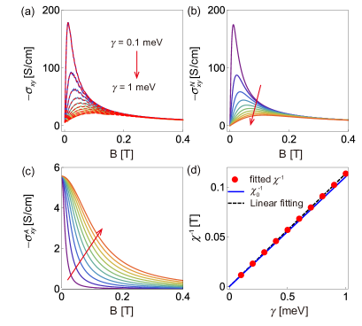
Figure 2: (a) Hall conductivity as a function of magnetic field for a constant spin splitting $\omega=3\,\mathrm{meV}$ and several selected band broadenings, the red dashed lines are the fitting curve from Eq. (10), and the solid lines are the numerical results from Eq. (3). (b) and (c) are the fitted orbital part and anomalous part of Hall conductivity in (a). (d) the inverse of fitted mobility as function of band broadenings, the blue lines are the inverse of mobility at $B=0$, $\chi_{0}=\frac{e\hbar}{2\gamma}\frac{v_{x}v_{y}}{(\mu+\omega)}$, and the dashed line is the linear fitting to $\chi^{-1}$.

III.3 Magnetic-field-dependent Zeeman splitting

For the magnetic-field-dependent Zeeman splitting, i.e., $\omega=\frac{1}{2}g\mu_{B}B$ with $g=20$, it is hard to distinguish the contribution of anomalous Hall conductivity and conventional orbital Hall conductivity. Setting a constant broadening width $\gamma=0.1\,\mathrm{meV}$ and carrier density $n_{0}=2.5\times 10^{15}\,\mathrm{cm^{-3}}$, following the same procedure, we can calculate the Hall conductivity with disorder effect, which has been given in Fig. 3. When the carrier density is fixed, as shown in Fig. 3(a), the chemical potential varies as a function of magnetic field, and it decreases monotonically in the strong magnetic field. Besides, the Hall conductivity can be described by the orbital Hall conductivity $\sigma_{xy}=\frac{\chi B\sigma_{D}}{1+\chi^{2}B^{2}}$ very well, as indicated by the blue line in Fig. 3(b). Similar to the constant spin-splitting case, the Hall conductivities with disorder effect coincide with the Hall conductivity in the clean limit [$\sigma_{xy}=-en_{0}/B$, the Green line in Fig. 3(b)] in the high field regime. Besides, we also calculate the Hall conductivity for several different band broadenings in Fig. 3(c), where the dip position shifts to the high magnetic field by increasing $\gamma$. The background of total Hall conductivity [solid lines] can be well-fitted by $\sigma_{xy}=\frac{\chi B\sigma_{D}}{1+\chi^{2}B^{2}}$ as indicated by the red dashed lines. The obtained mobility $\chi$ [red dots] has a good agreement with the mobility at zero magnetic field $\chi_{0}=\frac{e\hbar}{2\gamma}\frac{v_{x}v_{y}}{\mu}$ as shown in Fig. 3(d), where the Zeeman splitting is a higher order contribution in magnetic field to the Hall conductivity and negligible. In Appendix C, we further evaluate the transverse conductivity to obtain the Hall resistivity, we find the Hall resistivity is almost linear in magnetic field, which also does not show the signature of anomalous Hall effect.

Most previous works attribute the anomalous Hall effect to the Berry curvature effect due to the band degeneracy lifting by the Zeeman splitting. This effect can be evaluated based on a semiclassical approach by the integration of the Berry curvature and the magnetic field is only encoded in the energy level splitting for spin-up and spin-down electrons. However, in Dirac systems with large spin-orbital coupling which couples the spin-up and spin-down bands together, the magnetic field also introduces the vector potential that the canonical momentum is replaced by the kinetic momentum $\hbar\mathbf{k}\to\hbar\mathbf{k}+e\mathbf{A}$, leading to the formation of the Landau levels. The semiclassical approach completely ignores this part of contribution. In the full quantum mechanical approach here, we treat these two parts of contribution simultaneously. As previously discussed, The discrepancy between two approaches becomes more apparent for strong fields especially in the quantum limit where only the lowest Landau subband is filled and the semiclassical approach is completely inapplicable. In this regime, the Hall conductivity decreases as $B^{-1}$ as $B$ increases in quantum mechanical approach whereas saturates at high fields in semiclassical approach.

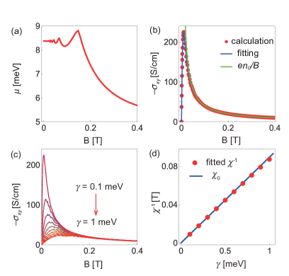
Figure 3: (a) By fixing the carrier density as $n_{0}=2.5\times 10^{15}\,\mathrm{cm}^{-3}$, the chemical potential $\mu$ is a function of magnetic field. (b) Hall conductivity as a function of magnetic field for Zeeman energy $\omega=\frac{1}{2}g\mu_{B}B$ and constant broadening $\gamma=0.1\,\mathrm{meV}$, the open circles are the numerical results, blue line is the fitting curve from the Hall conductivity $\sigma_{xy}=\frac{\chi B\sigma_{D}}{1+\chi^{2}B^{2}}$, and the green solid line represents the Hall conductivity in the clean limit. (c) Hall conductivity as a function of magnetic field for several selected band broadenings, the red dashed lines are the fitting curve from the Hall conductivity $\sigma_{xy}=\frac{\chi B\sigma_{D}}{1+\chi^{2}B^{2}}$, and the solid lines are the numerical results from Eq. (3). (d)The inverse of fitted mobility as function of band broadenings, the blue line are the inverse of mobility at $B=0$, $\chi_{0}=\frac{e\hbar}{2\gamma}\frac{v_{x}v_{y}}{\mu}$.

IV Possible origins

As the Zeeman effect has been excluded for the anomalous Hall effect, we expect a new mechanism for it. By summarizing the experiments in different works, we find that the anomalous Hall effect is more significant in thin film sample, which is usually several hundred nanometers. Consider the layer structure of $\mathrm{ZrTe_{5}}$ and small velocity along the $z$-direction, it can be regarded as a quasi-two dimensional system, and the localization effect may play important role in the Hall conductivity as in the pure two-dimensional system. Usually, the localization effect can be effectively considered by fixed chemical potential (QHE, ). In the clean limit and zero temperature, the carrier density in Eq. (8) becomes $n_{0}=\frac{k_{F,z}}{2\pi^{2}\ell_{B}^{2}}$ with $k_{F,z}$ the fermi wave vector of lowest Landau level. Then, plugging $n_{0}$ into Eq. (7), one obtained the Hall conductivity in the quantum limit as

$$\sigma_{xy}=-\frac{e^{2}}{2\pi^{2}\hbar}k_{F,z}.$$ (11)

It is noted that Eq. (11) is a general expression for the Hall conductivity in the quantum limit. Once $k_{F,z}$ is pinned to a constant due to the localization effect, $\sigma_{xy}$ is quasi-quantized. For density $n_{0}=\varrho\times 10^{15}\mathrm{cm}^{-3}$ at zero temperature and zero magnetic field, one has $k_{F,z}=(3\pi^{2}n_{0})^{1/3}\frac{(v_{x}v_{y}v_{z})^{1/3}}{v_{z}}$ and $B_{QL}\approx 0.314\frac{v_{z}}{(v_{x}v_{y}v_{z})^{1/3}}\varrho^{2/3}\,\mathrm{T}$, where the system enters the quantum limit for $B>B_{QL}$. In general, we expect that the critical field for Hall plateau is smaller than $B_{QL}$ due to the effect of disorder and temperature. This simple analysis is consistent with the experimental measurements, where the magnitude of Hall plateau and the corresponding critical field are increasing functions of carrier density in the low temperatures (Mutch2021arxiv, ).

As shown in Fig. 4, by fixing the chemical potential in the magnetic field, we present the Hall conductivity at different temperatures. There is a clear quasi-quantized structure in the Hall conductivity when the system enters the quantum limit regime. The magnitude of the plateau decreases with increasing temperature, and is almost independent of the band broadening. The oscillatory part of Hall conductivity is almost smeared out by a finite temperature. In addition, the Zeeman effect does not change the results qualitatively, and it only leads to the upward trend in the high magnetic field as shown in Fig. 4 (c). Moreover, we plot Eq. (11) and experimental data in literatures (sun2020npj, ; liu2021PRB, ; Mutch2021arxiv, ) together in Fig. 4 (d). Eq. (11) describes the carrier density dependence of Hall plateau value very well, which demonstrates that the observed Hall plateau can be attributed to the fixed chemical potential in magnetic field. Theoretically, the incommensurate charge density wave could offer one possible mechanism for the fixed chemical potential in $\mathrm{ZrTe}_{5}$ (tang2019nature, ; qin2020prl, ). However, the formation of charge density wave also requires the transverse conductivity vanishes in the corresponding magnetic field regime, which is inconsistent with the most of experimental measurements for $\mathrm{ZrTe_{5}}$ samples. Hence, it is anticipated that the fixed chemical potential is caused by mechanisms other than charge density wave, such as the localization effect from disorder (Rameshprb1990, ; Morgensternprb2001, ; Haudeprl2001, ). Besides, if there is charge transfer between the conduction band and other strongly scattering additional band, the carrier density in the conduction band can generically vary with field Gooth2022rpp . Correspondingly, the fermi wave vector $k_{F,z}$ might be field insensitive and is approximately a constant. The theoretical mechanism behind these scenarios requires further study in the future.

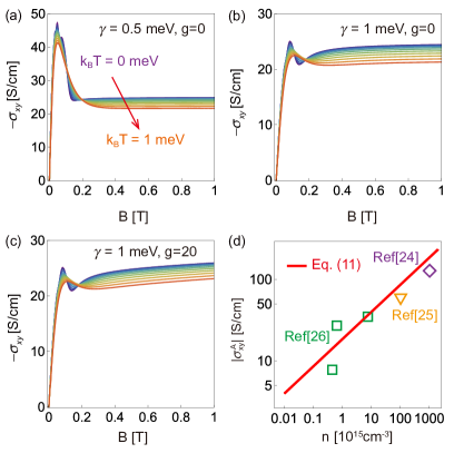
Figure 4: Hall conductivity as a function of the magnetic field for different temperatures. The band broadening is chosen as $\gamma=0.5\,\mathrm{meV}$ for (a) and (c) and $\gamma=1\,\mathrm{meV}$ for (b). The g-factor is chosen as $g=0$ for (a) and (b) and $g=20$ for (c). The carrier density in the absence of magnetic field is fixed as $n_{0}=2.5\times 10^{15}\,\mathrm{cm^{-3}}$ at different temperatures. The chemical potential is fixed by varying the magnetic field. (d) the comparison between Eq. (11) and experimental data in literatures.

V Summary and discussion

In summary, we have studied the Hall conductivity for $\mathrm{ZrTe}_{5}$ and $\mathrm{HfTe_{5}}$ based on the massive Dirac fermions. When Landau levels are formed in a finite magnetic field, there are two cases. (i) For a constant spin splitting, $\sigma_{xy}^{A}$ is finite and robust to the weak disorder at $B=0$, but vanishes in a high magnetic field and in the clean limit. (ii) For the magnetic field dependent Zeeman splitting $\omega=\frac{1}{2}\mu_{B}gB$, it is hard to identify the contribution of anomalous Hall conductivity from the total Hall conductivity. The Hall resistivity is almost linear in magnetic field even in the presence of Zeeman effect with a giant $g$-factor ($g=20$). Actually, the anomalous Hall effect for massive spin-split Dirac fermions are suppressed by a magnetic field by a factor $(1+\chi^{2}B^{2})^{-1}$ and vanishes in a finite magnetic field or in the clean limit as $(1+\chi^{2}B^{2})^{-1}\to 0$. Our calculations indicate that Zeeman field cannot generate the anomalous Hall effect in $\mathrm{ZrTe_{5}}$ and $\mathrm{HfTe_{5}}$. Even for constant Zeeman splitting, the anomalous Hall effect is suppressed in the strong magnetic field, and the calculation from the semiclassical treatment cannot be simply extended to the strong magnetic field. If the chemical potential is fixed in the magnetic field, there is a plateau in Hall conductivity, which might provide an explanation for the observed anomalous Hall effect in experiments.

Appendix A Anomalous Hall Conductivity without Landau level

In this section, we simply consider the case semi-classically, where the effect of magnetic field can be encoded into the Zeeman energy as $\omega=g_{z}\mu_{B}B/2$ with $g_{z}=21.3$ the g-factor and $\mu_{B}=5.788\times 10^{-2}\,\mathrm{meV\cdot T^{-1}}$ the Bohr magneton liu2016nc . Then, the low energy Hamiltonian in Eq. (1) becomes

$$H(k)=m\tau_{z}+\omega\sigma_{z}+v_{i}\hbar k_{i}\Gamma_{i}.$$ (12)

Solving the eigen equation, $H|\psi\rangle=\varepsilon|\psi\rangle$, we can find the energy spectrum as

$$\varepsilon_{s\zeta}=\zeta\sqrt{\left(m_{\perp}+s\omega\right)^{2}+\left(v_{z}\hbar k_{z}\right)^{2}},$$

where $m_{\perp}=\sqrt{m^{2}+\hbar^{2}\left(v_{x}^{2}k_{x}^{2}+v_{y}^{2}k_{y}^{2}\right)}$ , $s=\pm$ represents two splitting states because of the Zeeman effect, $\zeta=+$ is for the conduction band and $\zeta=-$ is for the valence band. The system becomes a nodal line semimetal when $\omega>m$, and the nodal ring is given by $\hbar^{2}\left(v_{x}^{2}k_{x}^{2}+v_{y}^{2}k_{y}^{2}\right)=\omega^{2}-m^{2}$ and $k_{z}=0$.

The corresponding eigenstates are found as

$$|\psi_{\lambda}\rangle=\begin{pmatrix}\zeta\cos\frac{\phi_{s\zeta}}{2}\cos\frac{\theta_{s}}{2}\\ s\mathrm{sign}(k_{z})\sin\frac{\phi_{s\zeta}}{2}\sin\frac{\theta_{s}}{2}e^{i\phi_{k}}\\ s\zeta\cos\frac{\phi_{s\zeta}}{2}\sin\frac{\theta_{s}}{2}e^{i\phi_{k}}\\ \mathrm{sign}(k_{z})\sin\frac{\phi_{s\zeta}}{2}\cos\frac{\theta_{s}}{2}\end{pmatrix}$$ ,

where the angles $\phi_{s\zeta}$, $\theta_{s}$ and $\phi_{k}$ are defined as $\cos\phi_{s\zeta}=\frac{\omega+sm_{\perp}}{\varepsilon_{s\zeta}}$, $\cos\theta_{s}=\frac{sm}{m_{\perp}}$ and $e^{i\phi_{k}}=\frac{v_{x}k_{x}+iv_{y}k_{y}}{\sqrt{v_{x}^{2}k_{x}^{2}+v_{y}^{2}k_{y}^{2}}}$. The subscript $\lambda$ denotes the quantum number $s$ and $\zeta$.

At the zero magnetic field, the anomalous Hall conductivity can be attributed to the nonzero Berry curvature of band structure as xiao2010rmp ; nagaosa2010rmp

$$\sigma_{xy}=\frac{e^{2}}{V\hbar}\sum_{k,\lambda}\Omega_{z}^{\lambda}n_{F}(\varepsilon_{\lambda}-\mu),$$ (13)

where $\Omega_{\ell}^{\lambda}$ is the $\ell$th component of Berry curvature vector of the $\lambda$th band. For well-separated bands, $\Omega_{\ell}^{\lambda}$ can be expressed as

$$\Omega_{\ell}^{\lambda}=\hbar^{2}\epsilon_{ij\ell}\sum_{\lambda^{\prime}\neq\lambda}\frac{\mathrm{Im}[v_{\lambda\lambda^{\prime}}^{i}v_{\lambda^{\prime}\lambda}^{j}]}{(\varepsilon_{\lambda}-\varepsilon_{\lambda^{\prime}})^{2}},$$

where $\epsilon_{ij\ell}$ is the Levi-Civita antisymmetric tensor with $i,j,\ell$ standing for $x,y,z$. $v_{\lambda\lambda^{\prime}}^{i}=\langle\psi_{\lambda}|\hat{v}^{i}|\psi_{\lambda^{\prime}}\rangle$ is the matrix element of velocity operator $\hat{v}^{i}$ in the eigen basis. For the massive Dirac fermions with Zeeman splitting, we can evaluate the $z$ component of Berry curvature as $\Omega_{z}^{\zeta s}=\frac{smv_{x}v_{y}\hbar^{2}}{2m_{\perp}^{3}}.$ Here $\Omega_{z}^{\zeta s}$ is independent of band index $\zeta$ and momentum $k_{z}$, and its sign depends on the band index $s$ and Dirac mass $m$. The magnitude of $\Omega_{z}^{\zeta s}$ is a decreasing function of $k_{\perp}$ and has a maximum at $k_{\perp}=0$ as $|\Omega_{z}^{\zeta s}(k_{\perp}=0)|=\frac{\hbar^{2}v_{x}v_{y}}{2m^{2}}$, and it vanishes as $k_{\perp}\to+\infty$. Then, we arrive the Hall conductivity as

$$\sigma_{xy}= e^{2}v_{x}v_{y}\hbar\sum_{s\zeta}\int\frac{d^{3}k}{(2\pi)^{3}}\frac{sm}{2m_{\perp}^{3}}n_{F}(\varepsilon_{s\zeta}-\mu)$$ (14)

It is easy to check that $\sigma_{xy}(-\mu,\omega)=-\sigma_{xy}(\mu,\omega)$ and $\sigma_{xy}(-\omega,\mu)=-\sigma_{xy}(\omega,\mu)$; hence, the anomalous Hall effect is asymmetric about the chemical potential and Zeeman energy. When the chemical potential is inside the band gap and temperature is zero, $n_{F}(\epsilon_{+\zeta}-\mu)=n_{F}(\epsilon_{-\zeta}-\mu)$, $\sigma_{xy}=0$; otherwise, $\sigma_{xy}(\omega\neq 0,\mu)\neq 0$. Besides, as $\varepsilon_{s\zeta}$ and $m_{\perp}$ are even in $m$, $\sigma_{xy}$ is odd in Dirac mass $m$ and vanishes when $m=0$. The finite Dirac mass is essential for the presence of anomalous Hall effect in $\mathrm{ZrTe}_{5}$. For simplicity, we put the chemical potential inside the conduction band $(\mu>0)$, and consider $\omega\geq 0$ and $m>0$ in the following discussion. At the zero temperature, Eq. (14) can be further simplified as

$$\sigma_{xy}= \frac{m}{2\pi\hbar v_{z}}\frac{e^{2}}{h}\sum_{s}\int_{|m|+s\omega}^{+\infty}dt\frac{s\sqrt{\mu^{2}-t^{2}}}{(t^{2}-s\omega)^{2}}\theta(\mu^{2}-t^{2})$$ (15)

where $\theta(x)$ is the unit-step function. We can define sum of the two integrals as $J$; then, $\sigma_{xy}=\frac{m}{2\pi\hbar v_{z}}\frac{e^{2}}{h}J$.

If we fix carrier density as a constant, $\mu$ is a function of $\omega$ and can be solved from the following equation,

$$n_{0}= \sum_{s,\chi=\pm}\int\frac{d^{3}k}{(2\pi)^{3}}\chi n_{F}(\varepsilon_{s}-\chi\mu).$$

For instance, we set $n_{0}=2.5\times 10^{15}\,\mathrm{cm^{-3}}$, the obtained chemical potential $\mu$ decreases with the increasing of $\omega$. There are two critical Zeeman energy, $\omega_{c1}$ and $\omega_{c2}$. As shown in Fig. 5(a), when $0<\omega<\omega_{1c},$ $\mu$ intersect with both bands of $s=+$ and $s=-$. When $\omega>\omega_{c1}$, $\mu$ intersects with band $s=-$ only. If $\omega$ is further larger than $\omega_{2}$, $\mu$ is lower than the band edge of $s=-$ at $k=0$.

Accordingly, there are three regimes for the nonzero $J$. When $\omega$ is smaller than $\omega_{c1}$,

$$J= \sum_{s}J_{s}(\omega,\mu)$$ (16)

where

$$J_{s}(\omega,\mu)= \frac{\omega}{\mu_{\omega}}\ln\left(\frac{\mu m}{\mu_{\omega}(\mu_{s}+\mu_{\omega})-s\omega m}\right)$$

$$+\frac{s\mu_{s}}{m}-s\cos^{-1}\left(\frac{m+s\omega}{\mu}\right)$$

with $\mu_{s}=\sqrt{\mu^{2}-(s\omega+m)^{2}}$ and $\mu_{\omega}=\sqrt{\mu^{2}-\omega^{2}}$. As indicated by the regime I in Fig. 5(a), the anomalous Hall conductivity is an decreasing function of $\omega$.

If we further increase the Zeeman energy so that $\omega_{c1}<\omega<\omega_{c2}$, the system enters the regime II in Fig. 5(a), the dimensionless coefficient $J$ becomes

$$J= J_{-}(\omega,\mu)$$ (17)

which is a increasing function of $\omega$.

If the Zeeman energy is so large that $\omega\geq\omega_{c2}$, as shown by the regime III in Fig. 5(a), the coefficient $J$ is found as

$$J= -\pi\left(\frac{\omega}{\sqrt{\omega^{2}-\mu^{2}}}-1\right)$$ (18)

which increases with the increasing of $\omega$ and approaches zero as $\omega\gg\mu$.

It is noted that $\sigma_{xy}$ reaches its max value when $\omega=\omega_{c1}$, and the corresponding maximum value are

$$\sigma_{xy}^{max}= \frac{m}{2\pi\hbar v_{z}}\frac{e^{2}}{h}J_{-}(\omega_{c1},\omega_{c1}+m)$$

For $m=5\,\mathrm{meV}$, $n_{0}=2.5\times 10^{15}\mathrm{cm^{-3}}$, $\omega_{c1}=2.65\,\mathrm{meV}$, $\frac{m}{2\pi\hbar v_{z}}\frac{e^{2}}{h}\approx 9.25\,\Omega^{-1}\cdot\mathrm{cm^{-1}}$, and $|\sigma_{xy}^{max}|\approx 5.63\,\Omega^{-1}\cdot\mathrm{cm^{-1}}$. Furthermore, $J_{-}(\omega_{c1},\omega_{c1}+m)$ can be written as a decreasing function of $\omega_{c}/m$. There are several ways to enlarge the magnitude of $\sigma_{xy}^{max}$. On the one hand, we can reduce the fermi velocity $v_{z}$, on the other hand, we can increase the carrier density so that $\omega_{c}$ can be enhanced as shown in Fig. 5(c). Besides, if we keep the ratio $\omega_{c}/m$ as a constant, $|\sigma_{xy}^{max}|$ will also increase with the increasing of Dirac mass $m$.

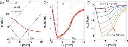
Figure 5: (a)Chemical potential and (b) Hall conductivity as a function of the Zeeman energy for a given carrier density. In (a), the dashed lines are the energy of the band edge of conduction bands at $k=0$. In (b), red open circles are numerically calculated from Eq. (14), the purple line is calculated by Eq. (16), the green line is calculated by Eq. (17), and the red line is calculated by Eq. (18). (c)The Hall conductivity as a function of the Zeeman energy for different given carrier density. The calculating parameters are chosen as $m=5\,\mathrm{meV}$.

Appendix B Landau level

In a finite perpendicular magnetic field $B$, in terms of the ladder operators $a$ and $a^{\dagger}$, the Hamiltonian in Eq. (1) can be expressed as

$$H=\begin{pmatrix}m+\omega&0&\eta a&v_{z}\hbar k_{z}\\ 0&m-\omega&v_{z}\hbar k_{z}&-\eta a^{\dagger}\\ \eta a^{\dagger}&v_{z}\hbar k_{z}&-m+\omega&0\\ v_{z}\hbar k_{z}&-\eta a&0&-m-\omega\end{pmatrix}.$$

For $n\geq 1$, using the ansatz $|\psi_{\lambda}\rangle=[c_{\lambda 1}|n-1\rangle,c_{\lambda 2}|n\rangle,c_{3\lambda}|n\rangle,c_{4\lambda}|n-1\rangle]^{T}$ with $n=1,2,3,\cdots$, we can solve out the eigen spectrum from the eigen equation $H|\psi_{\lambda}\rangle=\varepsilon_{\lambda}|\psi_{\lambda}\rangle$ as

$$\varepsilon_{n\zeta s}=\zeta\sqrt{(E_{n}+s\omega)^{2}+v_{z}^{2}\hbar^{2}k_{z}^{2}},$$

where $s=\pm$ represents two splitting states because of the Zeeman effect, $\zeta=+$ is for the conduction band and $\zeta=-$ is for the valence band, $E_{n}=\sqrt{m^{2}+n\eta^{2}}$. The corresponding eigen states are given by

$$|\psi_{\lambda}\rangle=\begin{pmatrix}\zeta\cos\frac{\phi_{ns\zeta}}{2}\cos\frac{\theta_{ns}}{2}|n-1\rangle\\ s\mathrm{sign}(k_{z})\sin\frac{\phi_{ns\zeta}}{2}\sin\frac{\theta_{ns}}{2}|n\rangle\\ s\zeta\cos\frac{\phi_{ns\zeta}}{2}\sin\frac{\theta_{ns}}{2}|n\rangle\\ \mathrm{sign}(k_{z})\sin\frac{\phi_{ns\zeta}}{2}\cos\frac{\theta_{ns}}{2}|n-1\rangle\end{pmatrix}$$ ,

where $\cos\phi_{ns\zeta}=\frac{\omega+sE_{n}}{\varepsilon_{ns\zeta}}$ and $\cos\theta_{ns}=\frac{sm}{E_{n}}$. The subscript $\lambda$ denotes the quantum number $n,s,\zeta$.

When $n=0$, we can find the eigen energy and eigen states as

$$\varepsilon_{0\zeta}=\zeta\sqrt{v_{z}^{2}\hbar^{2}k_{z}^{2}+(m-\omega)^{2}},$$

$$|\psi_{0\zeta}\rangle=\begin{pmatrix}0\\ \mathrm{sign}(k_{z})\sin\frac{\phi_{0\zeta}}{2}|0\rangle\\ \zeta\cos\frac{\phi_{0\zeta}}{2}|0\rangle\\ 0\end{pmatrix},$$

where $\cos\phi_{0\zeta}=\frac{\omega-m}{\varepsilon_{0\zeta}}$.

In the Landau level basis, the matrix element of velocity operator $v_{\lambda\lambda^{\prime}}^{i}$ can be evaluated as $v_{\lambda\lambda^{\prime}}^{i}=\langle\psi_{\lambda}|i\hbar^{-1}[H,r_{i}]|\psi_{\lambda^{\prime}}\rangle$. Along the $x-$ and $y-$ direction, the velocity operators are defined as $\hat{v}^{x}=i\hbar^{-1}[H,x]=v_{x}\Gamma_{1}$ and $\hat{v}^{y}=i\hbar^{-1}[H,y]=v_{y}\Gamma_{2}$, respectively. The product of matrix elements of $\hat{v}^{x}$ and $\hat{v}^{y}$ become,

$$v_{\lambda\lambda^{\prime}}^{x}v_{\lambda^{\prime}\lambda}^{y}= -i[v_{\lambda\lambda^{\prime}}^{(1)}]^{2}\delta_{n,n^{\prime}-1}+i[v_{\lambda^{\prime}\lambda}^{(1)}]^{2}\delta_{n,n^{\prime}+1}$$

$$v_{\lambda\lambda^{\prime}}^{x}v_{\lambda^{\prime}\lambda}^{x}= [v_{\lambda\lambda^{\prime}}^{(2)}]^{2}\delta_{n,n^{\prime}-1}+[v_{\lambda^{\prime}\lambda}^{(2)}]^{2}\delta_{n,n^{\prime}+1}$$

where $v_{\lambda\lambda^{\prime}}^{(1)}=\sqrt{v_{x}v_{y}}(c_{\lambda 3}c_{\lambda^{\prime}1}-c_{\lambda 2}c_{\lambda^{\prime}4})$ and $v_{\lambda\lambda^{\prime}}^{(2)}=v_{x}(c_{\lambda 3}c_{\lambda^{\prime}1}-c_{\lambda 2}c_{\lambda^{\prime}4})$. This relation can help us simplify the calculation for the Hall conductivity under finite magnetic field and temperature.

Besides, $G^{R/A}$ is diagonalized in the Landau level basis, and the diagonal elements are given by $G_{\lambda}^{R/A}=[\epsilon-\varepsilon_{\lambda}\pm i\gamma]^{-1}$,where $\lambda=n,s,\zeta$ denote the quantum numbers. By making the integral by parts for $\epsilon$ in Eq. (3), $\sigma_{xy}$ becomes

$$\sigma_{xy}= \frac{\hbar e^{2}}{\pi^{3}\ell_{B}^{2}}\sum_{\lambda\lambda^{\prime}}\int_{-\infty}^{+\infty}dk_{z}\int_{-\infty}^{+\infty}d\epsilon[v_{\lambda\lambda^{\prime}}^{(1)}]^{2}[-n_{F}^{\prime}(\epsilon-\mu)]$$

$$\times \frac{\delta_{n,n^{\prime}-1}}{2(\varepsilon_{\lambda}-\varepsilon_{\lambda^{\prime}})^{2}}\{\tan^{-1}\left(\frac{\varepsilon_{\lambda}-\epsilon}{\gamma}\right)+\tan^{-1}\left(\frac{\epsilon-\varepsilon_{\lambda^{\prime}}}{\gamma}\right)$$

$$-\frac{\gamma(\varepsilon_{\lambda}-\varepsilon_{\lambda^{\prime}})\left((\varepsilon_{\lambda}-\epsilon)(\varepsilon_{\lambda^{\prime}}-\epsilon)+\gamma^{2}\right)}{\left((\varepsilon_{\lambda}-\epsilon)^{2}+\gamma^{2}\right)\left((\varepsilon_{\lambda^{\prime}}-\epsilon)^{2}+\gamma^{2}\right)}\}$$

which is only contributed from the states near the fermi surface at the low temperature. In the weak scattering limit ($\gamma\to 0$), the terms in the big parentheses becomes $\frac{\pi}{2}[\mathrm{sgn}(\varepsilon_{\lambda}-\epsilon)+\mathrm{sgn}(\epsilon-\varepsilon_{\lambda^{\prime}})]$. After performing the integral of $\epsilon$, one arrives Eq. (4).

Appendix C Transverse conductivity and resistivity

As the magnitude of anomalous Hall conductivity is much smaller than the orbital Hall conductivity for $\omega=\frac{1}{2}g\mu_{B}B$, it is hard to see the anomalous contribution. To further confirm our conclusion in last part, we calculate the Hall resistivity to see wether there is a nonlinear behavior in the Hall curve or not. To obtain the elements of resistivity matrix, we need to further calculate the transverse conductivity $\sigma_{xx}$. According to the Kubo-Strda formula, the transverse conductivity $\sigma_{xx}$ in the Landau level basis is given by Mahan ; Streda1982 ; wang2018prb

$$\sigma_{xx}= \frac{e^{2}\hbar}{2\pi^{3}\ell_{B}^{2}}\sum_{\lambda\lambda^{\prime}}\int_{-\infty}^{+\infty}dk_{z}[v_{\lambda\lambda^{\prime}}^{(2)}]^{2}\delta_{n,n^{\prime}-1}$$

$$\int_{-\infty}^{\infty}[-n_{F}^{\prime}(\epsilon-\mu)]\text{Im}G_{\lambda}^{R}\text{Im}G_{\lambda^{\prime}}^{R}d\epsilon$$

Setting the calculation parameter identical to the one in main-text, we obtain the transverse conductivity as shown in Fig. 6(a), where the transverse conductivity decays quickly with the increasing of magnetic field and display an oscillating behavior for the moderate strong magnetic field. Besides, the transverse conductivity along $y$ direction can be obtained as $\sigma_{yy}=(\frac{v_{y}}{v_{x}})^{2}\sigma_{xx}$.

Taking advantage of the obtained Hall conductivity and transverse conductivity, we can derive the transverse and Hall resistivity as

$$\rho_{xx} =\frac{\sigma_{yy}}{\sigma_{xx}\sigma_{yy}+\sigma_{xy}^{2}},$$

$$\rho_{xy} =-\frac{\sigma_{xy}}{\sigma_{xx}\sigma_{yy}+\sigma_{xy}^{2}}.$$

As shown in Fig. 6(b), there are quantum oscillations in $\rho_{xx}$ and $\rho_{xy}$, and the oscillations split into two components in high magnetic field due to the Zeeman energy. The background of Hall resistivity is almost linear in magnetic field as $\rho_{xy}=\frac{B}{n_{0}e}$, which means there is no anomalous Hall effect due to the Zeeman energy. Besides, although the large transverse magneto-conductivity, there is almost no transverse magneto-resistivity. Hence, despite the Zeeman effect breaks the time-reversal symmetry, there is no linear magneto-resistivity in the weak magnetic field along the transverse configuration. For comparison, we also present the resistivity without Zeeman energy ($g=0$) as indicated by the black line in Fig. 6(b). There is no qualitative difference between the cases of $g=0$ and $g=20$. The Hall resistivity is also linear in magnetic field for both $g=0$ and $g=20$.

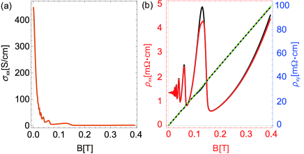
Figure 6: (a)Transverse conductivity as a function of magnetic field. (b)The resistivity (red and black line), Hall resistivity (blue line), and the linear background $B/n_{0}e$ (green line). For the resistivity, the $g$ factors are set as $g=20$ and $g=0$ for red and black line, respectively. For the Hall resistivity, the results of $g=20$ and $g=0$ are almost overlapped with each other, here we only present the result for $g=20$.

References

- (1) H. Weng, X. Dai, and Z. Fang, Transition-metal pentatelluride and : A paradigm for large-gap quantum spin Hall insulators, Phys. Rev. X 4, 011002 (2014).
- (2) R. Y. Chen, Z. G. Chen, X.-Y. Song, J. A. Schneeloch, G. D. Gu, F. Wang, and N. L. Wang, Magnetoinfrared Spectroscopy of Landau Levels and Zeeman Splitting of Three-Dimensional Massless Dirac Fermions in , Phys. Rev. Lett. 115, 176404 (2015).
- (3) Q. Li, D. E. Kharzeev, C. Zhang, Y. Huang, I. Pletikosic, A. V. Fedorov, R. D. Zhong, J. A. Schneeloch, G. D. Gu, and T. Valla, Chiral magnetic effect in , Nat. Phys. 12, 550 (2016).
- (4) Y. Zhang, C. Wang, L. Yu, G. Liu, A. Liang, J. Huang, S. Nie, X. Sun, Y. Zhang, B. Shen et al., Electronic evidence of temperature-induced Lifshitz transition and topological nature in , Nat. Commun. 8, 15512 (2017).
- (5) Y. Zhang, C. Wang, G. Liu, A Liang, L. Zhao, J. Huang, Q. Gao, B Shen, J. Liu, C. Hu et al., Temperature-induced Lifshitz transition in topological insulator candidate , Sci. Bull. 62, 950 (2017).
- (6) J. Mutch, W.-C. Chen, P. Went, T. Qian, I. Z. Wilson, A. Andreev, C. C. Chen, and J. H. Chu, Evidence for a strain-tuned topological phase transition in , Sci. Adv. 5, eaav9771 (2019).
- (7) P. Zhang, R. Noguchi, K. Kuroda, C. Lin, K. Kawaguchi, K. Yaji, A. Harasawa, M. Lippmaa, S. Nie, H. Weng et al., Observation and control of the weak topological insulator state in , Nat. Commun. 12, 406 (2021).
- (8) F. Tang, Y. Ren, P. Wang, R. Zhong, J. Schneeloch, S. A. Yang, K. Yang, P.A. Lee, G. Gu, Z. Qiao, and L. Zhang, Three-dimensional quantum Hall effect and metalinsulator transition in , Nature (London) 569, 537 (2019).
- (9) Y. Jiang, J. Wang, T. Zhao, Z. L. Dun, Q. Huang, X. S. Wu, M. Mourigal, H. D. Zhou, W. Pan, M. Ozerov, D. Smirnov, and Z. Jiang, Unraveling the Topological Phase of ZrTe 5 via Magnetoinfrared Spectroscopy, Phys. Rev. Lett. 125, 046403 (2020).
- (10) H. W. Wang, B. Fu, and S. Q. Shen, Helical symmetry breaking and quantum anomaly in massive Dirac fermions, Phys. Rev. B 104, L241111 (2021).
- (11) P. Wang, Y. Ren, F. Tang, P. Wang, T. Hou, H. Zeng, L. Zhang, and Z. Qiao, Approaching three-dimensional quantum Hall effect in bulk , Phys. Rev. B 101, 161201(R) (2020).
- (12) S. Galeski, X. Zhao, R. Wawrzynczak, T. Meng, T. Forster, P. M. Lozano, S. Honnali, N. Lamba, T. Ehmcke, A. Markou et al., Unconventional Hall response in the quantum limit of , Nat. Commun. 11, 5926 (2020).
- (13) S. Galeski, X. Zhao, R. Wawrzynczak, T. Meng, T. Forster, P. M. Lozano, S. Honnali, N. Lamba, T. Ehmcke, A. Markou et al., Origin of the quasi-quantized Hall effect in . Nat Commun. 12, 3197 (2021).
- (14) F. Qin, S. Li, Z. Z. Du, C. M. Wang, W. Zhang, D. Yu, H. Z. Lu, and X. C. Xie, Theory for the Charge-Density-Wave Mechanism of 3D Quantum Hall Effect, Phys. Rev. Lett. 125, 206601 (2020).
- (15) J. Gooth, S. Galeski, and T. Meng, Quantum-Hall physics and three dimensions, Rep. Prog. Phys. 86 044501 (2023).
- (16) Y. X. Wang, and Z. Cai, Quantum oscillations and three-dimensional quantum Hall effect in , Phys. Rev. B 107, 125203 (2023).
- (17) S. Okada, T. Sambongi, and M. Ido, Giant resistivity anomaly in , J. Phys. Soc. Jpn. 49, 839 (1980).
- (18) M. Izumi, K. Uchinokura, and E. Matsuura, Anomalous electrical resistivity in , Solid State Commun. 37, 641 (1981).
- (19) M. Izumi, K. Uchinokura, E. Matsuura, and S. Harada, Hall effect and transverse magnetoresistance in a low dimensional conductor , Solid State Commun. 42, 773 (1982).
- (20) T. M. Tritt, N. D. Lowhorn, R. T. Littleton Iv, A. Pope, C. R. Feger, and J. W. Kolis, Large enhancement of the resistive anomaly in the pentatelluride materials or with applied magnetic field, Phys. Rev. B 60, 7816 (1999).
- (21) M. Rubinstein, and : Possible polaronic conductors. Phys. Rev. B 60, 1627 (1999).
- (22) P. Shahi, D. J. Singh, J. P. Sun, L. X. Zhao, G. F. Chen, Y. Y. Lv, J. Li, J.-Q. Yan, D. G. Mandrus, J.-G. Cheng, Bipolar conduction as the possible origin of the electronic transition in pentatellurides: metallic vs semiconducting behavior. Phys. Rev. X 8, 021055 (2018).
- (23) T. Liang, J. Lin, Q. Gibson, S. Kushwaha, M. Liu, W. Wang, H. Xiong, J. A. Sobota, M. Hashimoto, P. S. Kirchmann et al., Anomalous Hall effect in , Nat. Phys. 14, 451 (2018).
- (24) Z. Sun, Z. Cao, J. Cui, C. Zhu, D. Ma, H. Wang, W. Zhuo, Z. Cheng, Z. Wang, X. Wan, and X. Chen, Large Zeeman splitting induced anomalous Hall effect in , Npj Quantum Mater. 5, 36 (2020).
- (25) Y. Liu, H. Wang, H. Fu, J. Ge, Y. Li, C. Xi, J. Zhang, J. Yan, D. Mandrus, B. Yan, et al., Induced anomalous Hall effect of massive Dirac fermions in and thin flakes, Phys. Rev. B 103, L201110 (2021).
- (26) J. Mutch, X. Ma, C. Wang, P. Malinowski, J. AyresSims, Q. Jiang, Z. Liu, D. Xiao, M. Yankowitz, and J.-H. Chu, Abrupt switching of the anomalous Hall effect by field-rotation in nonmagnetic , arXiv:2101.02681.
- (27) P. M. Lozano, G. Cardoso, N. Aryal, D. Nevola, G. Gu, A. Tsvelik, W. Yin, and Q. Li, Anomalous Hall effect at the Lifshitz transition in , Phys. Rev. B 106, L081124 (2022).
- (28) A. Gourgout, M. Leroux, J. L. Smirr, M. Massoudzadegan, R. P. S. M. Lobo, D. Vignolles, C. Proust, H. Berger, Q. Li, G. Gu et al., Magnetic freeze-out and anomalous Hall effect in , npj Quantum Mater. 7, 71 (2022).
- (29) Y. Choi, J. W. Villanova, and K. Park, Zeeman-splitting-induced topological nodal structure and anomalous Hall conductivity in , Phys. Rev. B 101, 035105 (2020).
- (30) D. Xiao, M. C. Chang, and Q. Niu, Berry phase effects on electronic properties, Rev. Mod. Phys. 82, 1959 (2010).
- (31) N. Nagaosa, J. Sinova, S. Onoda, A. H. MacDonald, and N. P. Ong, Anomalous Hall effect, Rev. Mod. Phys. 82, 1539 (2010).
- (32) B. Fu, H. W. Wang, and S. Q. Shen, Dirac Polarons and Resistivity Anomaly in and , Phys. Rev. Lett. 125, 256601(2020).
- (33) C. Wang, Thermodynamically Induced Transport Anomaly in Dilute Metals and , Phys. Rev. Lett. 126, 126601(2021).
- (34) A. A. Burkov and L. Balents, Weyl Semimetal in a Topological Insulator Multilayer, Phys. Rev. Lett. 107, 127205 (2011).
- (35) A. A. Zyuzin and A. A. Burkov, Topological response in Weyl semimetals and the chiral anomaly, Phys. Rev. B 86, 115133 (2012).
- (36) S. Q. Shen, Y. J. Bao, M. Ma, X. C. Xie, and F. C. Zhang, Resonant spin Hall conductance in quantum Hall systems lacking bulk and structural inversion symmetry, Phys. Rev. B 71, 155316 (2005).
- (37) A. B. Pippard, Magnetoresistance in Metals (Cambridge University Press, Cambridge, UK, 1989).
- (38) G. D. Mahan, Many-particle Physics.(Springer Science & Business Media, 2013).
- (39) P. Streda, Quantised Hall effect in a two-dimensional periodic potential, J. Phys. C: Solid State Phys. 15, L1299 (1982).
- (40) H. W. Wang, B. Fu, and S. Q. Shen, Intrinsic magnetoresistance in three-dimensional Dirac materials with low carrier density, Phys. Rev. B 98, 081202(R) (2018).
- (41) V. Yu. Tsaran and S. G. Sharapov, Magnetic oscillations of the anomalous Hall conductivity, Phys. Rev. B 93, 075430 (2016).
- (42) The Quantum Hall Effect, edited by R. E. Prange and S. M. Girvin (Springer-Verlag, New York, 1987).
- (43) G. M. Ramesh, Influence of localization on the Hall effect in narrow-gap, bulk semiconductors, Phys. Rev. B 41, 7922(R) (1990).
- (44) M. Morgenstern, D. Haude, Chr. Meyer, and R. Wiesendanger, Experimental evidence for edge-like states in three-dimensional electron systems, Phys. Rev. B 64, 205104 (2001).
- (45) D. Haude, M. Morgenstern, I. Meinel, and R. Wiesendanger, Local Density of States of a Three-Dimensional Conductor in the Extreme Quantum Limit, Phys. Rev. Lett. 86, 1582 (2001).
- (46) Y. Liu, X. Yuan, C. Zhang, Z. Jin, A. Narayan, C. Luo, Z. Chen, L. Yang, J. Zou, X. Wu et al., Zeeman splitting and dynamical mass generation in Dirac semimetal , Nat. Commun. 7, 12516 (2016).