Efficient Guided Generation for Large Language Models

Abstract

In this article we show how the problem of neural text generation can be constructively reformulated in terms of transitions between the states of a finite-state machine. This framework leads to an efficient approach to guiding text generation with regular expressions and context-free grammars by allowing the construction of an index over a language model’s vocabulary. The approach is model agnostic, allows one to enforce domain-specific knowledge and constraints, and enables the construction of reliable interfaces by guaranteeing the structure of the generated text. It adds little overhead to the token sequence generation process and significantly outperforms existing solutions. An implementation is provided in the open source Python library Outlines (Louf and Willard, ).

1 Introduction

We are concerned with the problem of generating sequences of tokens from a large language model (LLM) (Vaswani et al., 2017; Radford et al., 2019) that conform to regular expressions or context-free grammars (CFGs). This kind of guided LLM generation is used to make LLM model output usable under rigid formatting requirements that are either hard or costly to capture through fine-tuning alone (Beurer-Kellner et al., 2023; Scholak et al., 2021; Poesia et al., 2022a; Rabinovich et al., 2017; Weng, 2021; Dong et al., 2023; Poesia et al., 2022b; Geng et al., 2023; Wang et al., 2023). Such features have recently been generalized in prompting libraries and interfaces (Microsoft, 2023; Beurer-Kellner et al., 2023; Rickard, 2023a, b), but their applicability can be limited by their scaling costs.

Most implementations of guided generation bias the score values used to determine the probabilities of the tokens in an LLM’s vocabulary. A common and sufficient approach involves repeated evaluations over the entire vocabulary in order to determine which tokens are valid–according to the constraints and previously sampled tokens–and setting the probabilities of invalid tokens to zero. This approach entails a fixed $\mathcal{O}(N)$ cost for each token generated, where $N$ is the size of the LLM’s vocabulary.

We propose an approach that uses the finite state machine (FSM) formulation of regular expressions to both arbitrarily start and stop guided generation and allow the construction of an index with which the set of non-zero-probability tokens can be obtained efficiently at each step. The result is an algorithm that costs $\mathcal{O}(1)$ on average.

For the regular expression case, our approach shares the most similarity with Kuchnik et al. (2023), which uses a transducer formulation to obtain FSMs defined over a language model’s vocabulary, and these FSMs contain much of the same information and scaling benefits as the indices described here. Our approach does not require the complete transducer abstraction and can be used to more easily extend existing, efficient regular expression libraries without modifying the underlying automatons and their implementations.

More importantly, our indexing approach can also be extended to CFGs and $\operatorname{LALR}(1)$ parsers to allow for efficient guided generation according to popular data formats and programming languages (e.g. JSON, Python, SQL, etc.). The transition to parsing is made by way of augmentations to traditional $\operatorname{LALR}(1)$ parser components and operations, making it–again–an approach that can be used to extend existing parser implementations.

2 LLM Sampling and Guided Generation

Let $S_{t}=\left(s_{1}\dots s_{t}\right)$ represent a sequence of $t$ tokens with $s_{t}\in\mathcal{V}$, $\mathcal{V}$ a vocabulary, and $\lvert\mathcal{V}\rvert=N$. The vocabularies, $\mathcal{V}$, are composed of strings from a fixed alphabet (Sennrich et al., 2015) and $N$ is often on the order of $10^{4}$ or larger.

We define the next token $s_{t+1}$ as the following random variable:

$$\boldsymbol{\alpha} =\operatorname{LLM}(S_{t},\boldsymbol{\theta})$$

$$s_{t+1} \sim\operatorname{Categorical}({\boldsymbol{\alpha}})$$

where $\boldsymbol{\theta}$ is the set of trained parameters and $\boldsymbol{\alpha}\in\mathbb{R}^{N}$. In the context of this paper the function $\operatorname{LLM}$ refers to a deep neural network trained on next-token-completion tasks, but the method extends more generally to any function that takes token sequences and returns a probability distribution for the next token.

2.1 Sampling sequences

Let $\mathcal{F}\subset\mathcal{P}\left(\mathcal{V}\right)$, where $\mathcal{P}$ is the powerset operator, be subsets of multi-token strings that end with a special token $\texttt{EOS}\in\mathcal{V}$. The text generation task is to draw samples from $\mathcal{F}$.

Several procedures have been considered to generate elements of $\mathcal{F}$. Greedy decoding consists in generating tokens recursively, choosing the token with highest probability at each step. Beam search also generates tokens recursively, using a heuristic to find the mode of the distribution. More recently, SMC sampling has also been used to generate sequences (Lew et al., 2023).

Algorithm 1 Basic LLM token sampling

1:function sample_tokens($L$)

2:     $\boldsymbol{s}\leftarrow()$

3:     for $i\leftarrow 1,L$ do

4:         $\boldsymbol{\alpha}\leftarrow$ $\operatorname{LM}$($\boldsymbol{s}$, $\boldsymbol{\theta}$)

5:         Sample $s\sim\operatorname{Categorical}({\boldsymbol{\alpha}})$

6:         if $s=\texttt{EOS}$ then

7:              break

8:         end if

9:         $\boldsymbol{s}\leftarrow$ $\operatorname{append}$($\boldsymbol{s}$, $s$)

10:     end for

11:     return $\boldsymbol{s}$

12:end function

The sampling procedure is described in generality by Algorithm 1. Often called multinomial sampling, the procedure recursively generates new tokens by sampling from the categorical distribution defined above until the EOS token is found.

2.2 Guiding generation

We can derive other random variables from the next-token distribution by manipulating the output logits $\boldsymbol{\alpha}$. Since we are dealing with a finite, discrete distribution, we can compute an un-normalized conditional distribution by applying a boolean mask $m:\mathcal{P}\left(\mathcal{V}\right)\to\left\{0,1\right\}^{N}$ that restricts the support of the original distribution:

$$\boldsymbol{\alpha} =\operatorname{LM}(\tilde{S}_{t},\boldsymbol{\theta})$$

$$\tilde{\boldsymbol{\alpha}} =\operatorname{m}\left(\tilde{S}_{t}\right)\odot\boldsymbol{\alpha}$$

$$\tilde{s}_{t+1} \sim\operatorname{Categorical}({\tilde{\boldsymbol{\alpha}}})$$

The resulting conditional distribution implied by $\tilde{s}_{t+1}$ encodes constraints on the support of $s_{t+1}$. For instance, the masks $m$ could be designed so that the generated sequences, $\tilde{S}_{t+1}=\left(\tilde{s}_{1},\dots,\tilde{s}_{t+1}\right)$, represent

• digit samples,

• strings that match the regular expression [a-zA-Z],

• and strings that parse according to a specified grammar (e.g. Python, SQL, etc.)

The sampling procedure with masking is a simple augmentation of Algorithm 1 and is provided in Algorithm 2.

Algorithm 2 LLM token sampling with masking

1:function sample_tokens($L$)

2:     $\boldsymbol{s}\leftarrow()$

3:     for $i\leftarrow 1,L$ do

4:         $\boldsymbol{\alpha}\leftarrow$ $\operatorname{LLM}$($\boldsymbol{s}$, $\boldsymbol{\theta}$)

5:         Construct the mask $\operatorname{m}\left(\boldsymbol{s}\right)$

6:         $\tilde{\boldsymbol{\alpha}}\leftarrow\operatorname{m}\odot\boldsymbol{\alpha}$

7:         Sample $\tilde{s}\sim\operatorname{Categorical}({\tilde{\boldsymbol{\alpha}}})$

8:         if $\tilde{s}=\texttt{EOS}$ then

9:              break

10:         end if

11:         $\boldsymbol{s}\leftarrow$ $\operatorname{append}$($\boldsymbol{s}$, $\tilde{s}$)

12:     end for

13:     return $\boldsymbol{s}$

14:end function

The computation of $m$ on line $\ref{alg:llm-sequence-sampling-with-mask}.\ref{construct-m}$ is implicitly performed over all the elements of $\mathcal{V}$. Aside from computing $\boldsymbol{\alpha}$, this step is easily the most expensive. In the case of regular expression-guided masking–and cases more sophisticated than that–the support and, thus, $m$ will necessarily depend on the previously sampled tokens. Guided generation of this kind is ultimately an iterative matching or parsing problem and is not directly amenable to standard approaches that require access to a complete string upfront. In some cases, partial matching or parsing can be performed from the start of the sampled sequence on each iteration, but this has a cost that grows at least linearly alongside the $\mathcal{O}(N)$ cost of its application across the entire vocabulary.

This leads us to the main questions of this work: how can we efficiently match or parse incomplete strings according to a regular expression or CFG and determine the masks $m$ at each iteration of Algorithm 2?

3 Iterative FSM Processing and Indexing

We frame the case of regular expression guided generation in terms of state machines. This framing allows us to specify exactly how regular expression matching can be arbitrarily started and stopped, so that it can be easily and efficiently continued between samples of $\tilde{s}_{i+1}$, as well as how the masks can be computed without run-time evaluations over $\mathcal{V}$.

To be precise, we consider regular expressions in 5-tuple finite automaton form (Sipser, 1996, Definition 1.5):

Definition 1 (Finite Automaton).

A finite automaton, or finite-state machine, is given by $(Q,\Sigma,\delta,q_{0},F)$, where $Q$ is a finite set of states, $\Sigma$ a finite alphabet, $\delta:Q\times\Sigma\to Q$ the transition function, $q_{0}\in Q$ the start state, and $F\subseteq Q$ the set of accept states.

The characters comprising the strings in $\mathcal{V}$ are drawn from $\Sigma$: i.e. $\mathcal{V}\subset\mathcal{P}(\Sigma)$. Throughout, the FSM states, $Q$, will be represented by integer values for simplicity.

This formulation allows us to determine the exact states in $Q$ in which the guiding regular expression’s FSM stops after sampling a single vocabulary token $\tilde{s}_{t+1}$. These FSM states can then be tracked during the LLM token sampling process in Algorithm 2 and used to efficiently continue the state machine without reading from the beginning of the growing sample sequence each time.

Example 1.

We illustrate the FSM sampling process in 1 for the regular expression ([0-9]*)?\.?[0-9]*, which can be used to generate floating-point numbers. For simplicity, let the vocabulary, $\mathcal{V}$, consist of only the strings: "A"}, \mintinlinepython

”.”, "42"}, \mintinlinepython”.2”, and

"1"}.
When the generation begins, the FSM is in state \texttt

0, so our algorithm masks the string

"A"}, since it would not be accepted by the FSM.  We can only
sample \mintinline

python”.”, "42"}, \mintinlinepython”.2”, and

"1"} in this case.
If we sample \mintinline

python”.2”, we advance the FSM to state 3. In this case, only

"42"}
and \mintinline

python”1” are valid completions, so we mask the other values before sampling. If we sample "1"} instead, we advance the FSM to state \texttt1, in which case "."}, \mintinlinepython”.42”, ".2"}, and \mintinlinepython”1” are valid completions and the mask remains unchanged.

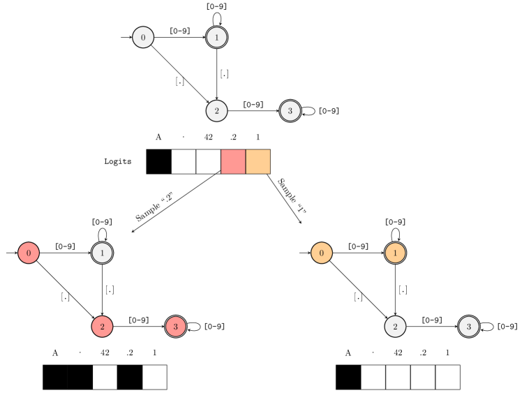
Figure 1: FSM masking for the regular expression ([0-9]*)?\.?[0-9]*.

Looping through the vocabulary to determine the valid next tokens is still the biggest issue. For that, we pre-process the vocabulary using the regular expression’s FSM and build an index. The important part is that we consider starting in every viable FSM state, because the strings in the vocabulary could match arbitrary parts of a regular expression, and those parts are implicitly the FSM states. A procedure for producing matches starting at any point in the FSM is given in 3. The result is a list of sub-sequences detailing the states through which the FSM would traverses when accepting the provided string.

Algorithm 3 Find sub-sequences of the FSM $M$ that accept the string $\boldsymbol{v}$

1:function find_sub_sequences($M$, $\boldsymbol{v}$)

2:     $M=(Q,\Sigma,\delta,q_{0},F)$

3:     $res\leftarrow()$

4:     for $r\in\delta^{-1}(\cdot,v_{0})$ do $\triangleright$ Loop through states that read $v_{0}$

5:         $p\leftarrow(r)$

6:         for $i\leftarrow 1,\lvert\boldsymbol{v}\rvert-1$ do $\triangleright$ Walk the FSM

7:              if $\delta(r,v_{i})=\emptyset$ then $\triangleright$ The FSM does not read $v_{i}$

8:                  $p\leftarrow()$

9:                  break $\triangleright$ Stop walking and try the next start state

10:              end if

11:              $r\leftarrow\delta(r,v_{i})$

12:              $p\leftarrow$ $\operatorname{append}$($p$, $r$)

13:         end for

14:         $res\leftarrow$ $\operatorname{append}$($res$, $p$)

15:     end for

16:     return $res$

17:end function

By matching the starting states of these sub-sequences to the last FSM state arrived at in a single step of the loop in Algorithm 2, we can efficiently index the vocabulary with a map, $\sigma:Q\to\mathcal{P}(\mathcal{V})$, connecting FSM states and sets of elements of the vocabulary that will be accepted by the FSM in those states. 4 describes the construction of $\sigma$.

Algorithm 4 Construct a map from FSM states to subsets of $\mathcal{V}$

1:function map_states_to_vocab($M$, $\mathcal{V}$)

2:     $M=(Q,\Sigma,\delta,q_{0},F)$

3:     Initialize the map $\sigma$ with empty sets for each element in $Q$

4:     for $v\in\mathcal{V}$ do $\triangleright$ Loop through the vocabulary

5:         $Z\leftarrow$ $\operatorname{find\_sub\_sequences}$($M$, $v$)

6:         for $z\in Z$ do $\triangleright$ Loop through state sequences accepting $v$

7:              $\sigma(z_{0})\leftarrow\sigma(z_{0})\cup v$

8:         end for

9:     end for

10:     return $\sigma$

11:end function

Using a hash-map for $\sigma$ can make the $m$ step in Algorithm 2 cost only $\mathcal{O}(1)$ on average. Furthermore, since $\sigma$ is constructed outside of the token sampling procedure, its run-time cost is effectively irrelevant, although it theoretically requires memory equal to the number of states in the FSM (i.e. $\lvert Q\rvert$). Fortunately, for non-pathological combinations of regular expressions and vocabularies, not every string in the vocabulary will be accepted by the FSM, and not every FSM state will be represented by a string in $\mathcal{V}$.

3.1 Examples

In this section we use GPT2-medium (355M parameters) to illustrate how regular expression guided generation works in practice. We use the library Outlines to generate them: minted language=python, nofloat import outlines.models as models import outlines.text.generate as generate model = models.transformers(”gpt2-medium”) prompt = ”Is 1+1=2? ” unguided = generate.continuation(model, max_tokens=30)(prompt) guided = generate.regex(model, r”s*([Yy]es—[Nn]o—[Nn]ever—[Aa]lways)”, max_tokens=30)( prompt ) print(unguided) # Is 1+1=2? # # This is probably the most perplexing question. As I said in one of my articles describing how I call 2 and 1, there isn’t print(guided) # Is 1+1=2? Always minted language=python, nofloat prompt = ”In what year was Noam Chomsky born?n” unguided = generate.continuation(model, max_tokens=30)(prompt) guided = generate.regex(model, r”s*19[0-9]2”, max_tokens=30)(prompt) print(unguided) # In what year was Noam Chomsky born? # # Professor Chomsky was born in about 1895 in Mille Medad, near Paris. Like others Chomsky does not know the details of the birth weight of print(guided) # In what year was Noam Chomsky born?1952 minted language=python, nofloat prompt = ”What is the IP address of the Google DNS servers? ” unguided = generate.continuation(model, max_tokens=30)(prompt) guided = generate.regex( model, r”((25[0-5]—2[0-4]d—[01]?dd?))̇3(25[0-5]—2[0-4]d—[01]?dd?)”, max_tokens=30, )(prompt) print(unguided) # What is the IP address of the Google DNS servers? # # Passive DNS servers are at DNS servers that are private. In other words, both IP servers are private. The database does not contain Chelsea Manning print(guided) # What is the IP address of the Google DNS servers? # 2.2.6.1

3.2 Comparison with current methods

To illustrate the efficiency of the indexing approach described here, and implemented in Outlines, we perform a simple comparison with the Guidance library. As of this writing, the Guidance library uses partial regular expression matching–applied from the start of the sampled sequence each time–and must iterate over the LLM’s vocabulary ($N=50,257$) on each step. The Guidance code and prompt used for this comparison are as follows: minted language=python, nofloat import guidance llm = guidance.llms.Transformers( ”gpt2”, token_healing=False, device=”cuda”, temperature=0.1, ) program = guidance( f”””What is a good Python variable name?gen temperature=0.1 max_tokens=max_tokens pattern=”[^Wd]w*””””, llm=llm, caching=False, async_mode=False, stream=False, log=False, silent=True, ) # Generate the token sequence. # Only this call is timed. program().text The corresponding Outlines code is as follows: minted language=python, nofloat from outlines import disable_cache import outlines.models as models import outlines.text.generate as generate disable_cache() model = models.transformers(”gpt2”, device=”cuda”, temperature=0.1) prompt = ”What is a good Python variable name? ” guided_continuation = generate.regex( model, r”[^Wd]w*”, max_tokens=max_tokens, ) def reset_continuation(): # This allows us to sample new sequences on each call guided_continuation.pstates = [] return guided_continuation(prompt) # Generate the token sequence. # Only this call is timed. reset_continuation() The value of max_tokens} is varied and the timings are recorded with \mintinlinepythontimeit for a single loop and single repeat value (i.e. only one sample is collected for each value of max_tokens}). The results are plotted in \Creffig:plot-guidance-comparisons. Barring any configuration oversights that might be creating a large run-time discrepancy, the observed scaling in the maximum number of sampled tokens is striking and is indicative of the growing computational problem implied by the approach.

4 Extensions to Iterative Parsing

In this section, we move our focus to general parser-guided generation and start with a simple walk-through for a Python-like grammar provided as a CFG. Consider a vocabulary consisting of strings like "d"} and \mintinlinepython”ef” that can be combined to produce Python-like syntax according to an implicit CFG, and assume that these strings are sequentially sampled and concatenated according to a process like Algorithm 1. Furthermore, consider a terminal symbol DEF in the CFG that corresponds to the string "def"} and is given by the trivial regular expression \textttdef. Also, consider a NAME symbol given by the regular expression [^\W\d]\w* (e.g. Python identifiers). We want to sequentially parse strings sampled from the aforementioned vocabulary in a way that adheres the Python syntax. For example, the following could be one such sequence:

["d", "ef", " f", "oo(", "):", " ", "pass"]}.  All the elements of the
sequence are by definition elements of the vocabulary.  Concatenating the sequence
produces \mintinline

python”def foo(): pass”, which is a valid sequence of tokens defining a function. In the situation we’re considering, we will have observed all the tokens up to a certain point and know nothing about the ones after that point. For instance, at the third observation in the example sequence, we have the concatenated string

"def f"}.  If we were to lex/parse this string a
traditional approach would return the symbol sequence \texttt

DEF NAME, which misidentifies the "f"} as a complete \textttNAME token. As we can see from the rest of the sequence, the correct NAME token will be

"foo"}.
In general, the next valid strings that can be sampled from the vocabulary are
ones that either
\begin

enumerate continue expanding/advancing the NAME currently starting with

"f"} (as the
full sequence in our example does), and/or
\item anything that begins with \mintinline

python”(”–i.e. an LPAR symbol with regular expression (–and proceeds to specify a valid argument signature. In the first case, the "f"} can be seen as a partially matched \textttNAME symbol in Python, and–recalling that its regular expression is [^\W\d]\w*–we can say that it matches both sub-patterns (i.e. [^\W\d] and \w*) in the regular expression. Our use of FSMs formalize the notion of sub-patterns by way of an FSM’s states. In this case, the regex for NAME can be represented by an FSM, $M$, with three states: 0 (i.e. the initial state $q_{0}$), 1 (i.e. [^\W\d]), and 2 (i.e. \w*), where $1,2\in F$. Using 3, we would obtain the FSM state sequences $(0,1)$, $(1,2)$, $(2,2)$ for "f"} and the FSM, \(M\), corresponding to the \textttNAME symbol. These FSM sequences for

"f"} tell us that matching can start for this
vocabulary string in the states 0, 1, or 2, and it can end in states 1 or 2.
According to case 1. above, parsing can be continued--for the \texttt

NAME symbol–after previously ending in states 1 or 2. According to case 2., the next string could also start with or contain an LPAR, implying that $M$ would have terminated, which it can given that 1 and 2 are final states in $M$ at which the parsing would have stopped after reading

"f"}.
\(M\) terminating also indicates that a \texttt

NAME symbol was completed, and that a transition to a state accepting LPAR was allowed by the grammar. In this illustration, the next valid vocabulary strings are at least

"d", "ef", "pass", " ", "oo("}, because all of those strings would expand the
partially matched \texttt

NAME, and the last one would also progress the parse state to one that reads an LPAR. The remaining string,

"):"}, from the subset of
the vocabulary we’ve considered would result in a sequence with invalid syntax.
In relation to the FSM indexing approach, this means that \Cref

alg:fsm-index-map would map FSM states 0, 1, and 2 to the subset

"d", "ef", "pass", " ", "oo("}
for the symbol \texttt

NAME and its FSM, $M$. This illustration omits the underlying parser states that determine which grammar symbols and transitions are allowed. We use pushdown automata (PDA) as a means to extend the FSM approach and address the remaining details.

4.1 Pushdown Automata Formulation

We define pushdown automata using the following 6-tuple representation (Sipser, 1996, Definition 2.13):

Definition 2 (Pushdown Automaton).

A pushdown automaton is given by $(Q,\Sigma,\Gamma,\delta,q_{0},F)$, where $Q$, $\Sigma$, $\Gamma$, and $F$ are all finite sets, $\Gamma$ is the stack alphabet, $\delta:Q\times\Sigma_{\epsilon}\times\Gamma_{\epsilon}\to\mathcal{P}\left(Q\times\Gamma_{\epsilon}\right)$, $\Gamma_{\epsilon}\equiv\Gamma\cup\epsilon$, $\epsilon$ is the empty character, and the remaining symbols retain their meanings from the finite automaton definition.

In order to construct an indexing approach for a PDA-driven parser, we need to use the connection between a CFG’s symbols–via a corresponding PDA’s alphabet–and the lexing and scanning steps that produce the symbols read by a PDA. More specifically, parsers are supported by lexers and scanners that identify symbols from a sequence of character inputs, as we implicitly illustrated in 4. Ordered lists of terminal symbols can be constructed for each parse/PDA state based on the symbol and stack transitions allowed by the map $\delta$ in each state. This means that we can construct an FSM for each parse state that is the union of each FSM corresponding to a terminal symbols read by the state. A scanning step will then identify a set of possible terminal symbols $V\subset\Sigma$ for the characters read since the last fully identified symbol in the parsing process. For example, in the initial state $q_{0}$ of a PDA for the Python-like CFG in 4, scanning and lexing the string

"de"} will
result in \(V = \left\

DEF, NAME }: i.e. DEF for any vocabulary string completing the string

"def"}--followed by a string not
also read by the \texttt

NAME FSM (e.g. "def "})--and \textttNAME for any other strings read by its FSM (e.g.

"default"}).
Note that steps of the scanner--and sampling steps of the LLM--will
eventually reduce the set \(V\) until a single terminal symbol \(v \in V\) is
determined.
By applying \Cref

alg:fsm-sub-sequences to each string in $\mathcal{V}$ using the combined FSMs for each parse state, we can determine parser configurations that consist of the PDA states, the corresponding FSM states, and the potential terminal symbols. By analogy with the steps in 3, we can use the pre-image of the PDA’s transition map to determine PDA stack values that will read the PDA states $q\in Q$ and terminal symbol sets $V$ of a parser configuration:

$$\delta^{-1}(q,V,\cdot)\equiv\left\{g:\delta(q,v,g)\in\mathcal{P}\left(Q\times\Gamma_{\epsilon}\right),g\in\Gamma_{\epsilon},v\in V\right\}.$$

The stack values provided by this map are needed in order to find paths–if any–through the PDA that allow successful, complete parses of each string in $\mathcal{V}$ starting from their possible parser configurations. For parser state and terminal combinations that correspond to REDUCE operations of an LALR(1) parser, these parser configurations will consist of more than just the top-of-stack values in $\Gamma$; they will consist of sub-stacks corresponding to all valid prefixes for the REDUCE operations entailed by a vocabulary string. Ultimately, each parser configuration that permits a complete parse of a vocabulary string is added as an entry in the index for the PDA, and, in this case, the index will need to be a trie data structure in order to allow queries against the parser’s stack values.

5 Discussion

The vocabulary indexing introduced in this paper removes a prohibitive run-time scaling barrier in guided generation. Naturally, it makes a trade-off between processing and memory, but we believe that the memory costs are relatively low on average and–when not–can be reduced through conventional means. In our tests using a slightly augmented version of the Python grammar, we find that even naively constructed indices (i.e. ones containing unused and redundant parser and FSM state configurations) are still only around 50 MB. Furthermore, these indices were constructed with un-reduced DFAs, implying that there are numerous redundant states unnecessarily increasing the size of the indices. Likewise, if the exact representation of the state machines is ever an issue, it’s possible that other state machine formulations with lower memory requirements could suffice (e.g. NFAs). The implications of this work are not limited to neural text generation. For instance, one could use the indexing approach described here to assist with the training or fine-tuning of LLMs when structured outputs are required. We can also speculate that assisted generation during training may reduce the need for a model to learn syntactic details. In addition, this method provides an alternative way to evaluate current models. One could, for instance, attempt to quantify the discrepancy between the masked logits generated by our method and the raw logits generated by the model. Which could in turn inform the training objective of a model. It may also be possible to “lift” the masks computed by this approach into the language models themselves. Basically, the masks implicitly determine which computations do not need to be performed. Our current formulation only applies the masks at the lowest level, but, by lifting the masks further up into the architecture of the model, we may be able to modulate which slices of the model parameters are needed before unnecessarily performing operations on them. This has the potential to further reduce computational costs.

References

- Beurer-Kellner et al. [2023] Luca Beurer-Kellner, Marc Fischer, and Martin Vechev. Prompting is programming: A query language for large language models. Proceedings of the ACM on Programming Languages, 7(PLDI):1946–1969, 2023.
- Dong et al. [2023] Yihong Dong, Ge Li, and Zhi Jin. CODEP: Grammatical Seq2Seq Model for General-Purpose Code Generation. In Proceedings of the 32nd ACM SIGSOFT International Symposium on Software Testing and Analysis, ISSTA 2023, pages 188–198, New York, NY, USA, July 2023. Association for Computing Machinery. ISBN 9798400702211. doi: 10.1145/3597926.3598048.
- Geng et al. [2023] Saibo Geng, Martin Josifosky, Maxime Peyrard, and Robert West. Flexible Grammar-Based Constrained Decoding for Language Models, May 2023.
- Kuchnik et al. [2023] Michael Kuchnik, Virginia Smith, and George Amvrosiadis. Validating large language models with relm. Proceedings of Machine Learning and Systems, 5, 2023.
- Lew et al. [2023] Alexander K. Lew, Tan Zhi-Xuan, Gabriel Grand, and Vikash K. Mansinghka. Sequential Monte Carlo Steering of Large Language Models using Probabilistic Programs. arXiv preprint arXiv:2306.03081, 2023.
- [6] Rémi Louf and Brandon T. Willard. Outlines: Generative Model Programming. URL https://github.com/normal-computing/outlines.
- Microsoft [2023] Microsoft. Guidance. Microsoft, July 2023. URL https://github.com/microsoft/guidance.
- Poesia et al. [2022a] Gabriel Poesia, Oleksandr Polozov, Vu Le, Ashish Tiwari, Gustavo Soares, Christopher Meek, and Sumit Gulwani. Synchromesh: Reliable code generation from pre-trained language models. arXiv preprint arXiv:2201.11227, 2022a.
- Poesia et al. [2022b] Gabriel Poesia, Oleksandr Polozov, Vu Le, Ashish Tiwari, Gustavo Soares, Christopher Meek, and Sumit Gulwani. Synchromesh: Reliable code generation from pre-trained language models, January 2022b.
- Rabinovich et al. [2017] Maxim Rabinovich, Mitchell Stern, and Dan Klein. Abstract syntax networks for code generation and semantic parsing. arXiv preprint arXiv:1704.07535, 2017.
- Radford et al. [2019] Alec Radford, Jeffrey Wu, Rewon Child, David Luan, Dario Amodei, and Ilya Sutskever. Language models are unsupervised multitask learners. OpenAI blog, 1(8):9, 2019.
- Rickard [2023a] Matt Rickard. parserLLM, July 2023a. URL https://github.com/r2d4/parserllm.
- Rickard [2023b] Matt Rickard. R2d4/rellm: Exact structure out of any language model completion., 2023b. URL https://github.com/r2d4/rellm.
- Scholak et al. [2021] Torsten Scholak, Nathan Schucher, and Dzmitry Bahdanau. PICARD: Parsing incrementally for constrained auto-regressive decoding from language models. arXiv preprint arXiv:2109.05093, 2021.
- Sennrich et al. [2015] Rico Sennrich, Barry Haddow, and Alexandra Birch. Neural machine translation of rare words with subword units. arXiv preprint arXiv:1508.07909, 2015.
- Sipser [1996] Michael Sipser. Introduction to the Theory of Computation. International Thomson Publishing, 1996.
- Vaswani et al. [2017] Ashish Vaswani, Noam Shazeer, Niki Parmar, Jakob Uszkoreit, Llion Jones, Aidan N. Gomez, \Lukasz Kaiser, and Illia Polosukhin. Attention is all you need. Advances in neural information processing systems, 30, 2017.
- Wang et al. [2023] Bailin Wang, Zi Wang, Xuezhi Wang, Yuan Cao, Rif A. Saurous, and Yoon Kim. Grammar Prompting for Domain-Specific Language Generation with Large Language Models, May 2023.
- Weng [2021] Lilian Weng. Controllable Neural Text Generation, January 2021. URL https://lilianweng.github.io/posts/2021-01-02-controllable-text-generation/.
Acknowledgments
We would like to thank Dan Gerlanc and Dan Simpson for their support and constructive feedback.