The Connection Between R-Learning and Inverse-Variance Weighting for Estimation of Heterogeneous Treatment Effects

Abstract

Many methods for estimating conditional average treatment effects (CATEs) can be expressed as weighted pseudo-outcome regressions (PORs). Previous comparisons of POR techniques have paid careful attention to the choice of pseudo-outcome transformation. However, we argue that the dominant driver of performance is actually the choice of weights. For example, we point out that R-Learning implicitly performs a POR with inverse-variance weights (IVWs). In the CATE setting, IVWs mitigate the instability associated with inverse-propensity weights, and lead to convenient simplifications of bias terms. We demonstrate the superior performance of IVWs in simulations, and derive convergence rates for IVWs that are, to our knowledge, the fastest yet shown without assuming knowledge of the covariate distribution.

1 Introduction

Estimates of conditional average treatment effects (CATEs) allow for treatment decisions to be tailored to the individual. Formally, let $A\in\{0,1\}$ be a binary treatment, let $X\in\mathcal{X}$ be a vector of confounders and treatment effect modifiers, let $Y_{(a)}$ be the potential outcome under treatment $a$, and let $Y=AY_{(1)}+(1-A)Y_{(0)}$ be the observed outcome. The CATE is defined as $\tau(X):=\mathbb{E}\left(Y_{(1)}-Y_{(0)}|X\right)$. Under conventional assumptions of exchangeability and positivity, the CATE can be identified as $\tau(x)=\mathbb{E}\left(Y|X,A=1\right)-\mathbb{E}\left(Y|X,A=0\right)$.

CATE estimation has a rich history going back several decades (see, e.g., Robins & Rotnitzky, 1995; Hill, 2011; Zhao et al., 2012; Imai & Ratkovic, 2013; Athey & Imbens, 2016; Hahn et al., 2017). We focus here on two general approaches: pseudo-outcome regression (POR) and R-learning. Both approaches easily accommodate flexible machine learning tools, and can attain double robustness (DR) properties similar to those established in the average treatment effect (ATE) literature (Kennedy, 2022a; Nie & Wager, 2020; see also Scharfstein et al. 1999; Robins et al. 2000; Bang & Robins 2005; Chernozhukov et al. 2022b; Kennedy 2022b)

POR aims to derive a noisy but unbiased approximation of $Y_{(1)}-Y_{(0)}$, and to fit a regression to predict this approximation using $X$ (Rubin & van der Laan, 2005; van der Laan, 2006; Tian et al., 2014; Chen et al., 2017; Foster & Syrgkanis, 2019; Künzel et al., 2019; Semenova & Chernozhukov, 2020; Curth & van der Schaar, 2021; see also Buckley & James 1979; Fan & Gijbels 1994; Rubin & van der Laan 2007; Díaz et al. 2018). The approximation of $Y_{(1)}-Y_{(0)}$ is referred to as a “unbiasing transformation” or “pseudo-outcome” because it serves as an observed stand-in for the latent outcome of interest $Y_{(1)}-Y_{(0)}$. For example, if the propensity scores $\text{Pr}(A=1|X)$ are known, then an appropriate pseudo-outcome can be derived using inverse propensity weights: $f_{\text{IPW}}(A,Y):=AY/\text{Pr}(A=1)-(1-A)Y/\text{Pr}(A=0)$. Since $\mathbb{E}\left(f_{\text{IPW}}(A,Y)|X\right)=\tau(X)$, regressing the pseudo-outcomes $f_{\text{IPW}}(A,Y)$ against $X$ produces a sensible estimate of $\tau$ (Powers et al., 2018). This regression can be done with any off-the-shelf machine learning algorithm. For this reason, POR methods are sometimes referred to as “meta-algorithms” (Kennedy, 2022a).

R-learning estimates the CATE using a moment condition derived by Robinson (1988; see Section 5.2 of Robins et al., 2008; Semenova et al., 2017; Nie & Wager, 2020; Zhao et al., 2022; Kennedy, 2022a; Kennedy et al., 2022). While R-Learning is sometimes described as separate from POR, it can also be expressed as a weighted POR (see Section 1.1, below, and the NonParamDML method in the EconML package from Syrgkanis et al. 2021).

This parallel between R-learning and weighted POR invites the question of whether or not weights should be used in POR more broadly, and, if so, what choice of weights is optimal? In other words, even after confounding bias has been accounted for through a pseudo-outcome transformation (e.g., $f_{\text{IPW}}$), should additional weights be used to prioritize the fit of $\tau$ of different subregions of $\mathcal{X}$? We aim to shed light on this question through a combination of simulation & theory.

Contribution Summary

The main intuition of this manuscript is that pseudo-outcomes based on inverse-propensity weights are effective at removing confounding, but can be unstable in the face of propensity scores close to zero or one. Inverse-variance weights restabilize the POR without reintroducing confounding, since the CATE estimand is conditional on $X$, and $Y$ is unconfounded within strata of $X$. This form of reweighting is done implicitly by the R-Learner.

Section 1.1 discusses the above intuition in more detail. Section 2 shows that the intuition bears out in simulations. Section 3 demonstrates how the framework of weighted POR can be used to study bias terms for CATE estimates, and to derive fast convergence rates. We close with a discussion.

1.1 Stabilizing weights in CATE estimation

In this section we outline connections between R-Learning and inverse-variance weighting (IVW). Let $Z:=(Y,X,A)$, and let

$$\mu_{a}(X) =\mathbb{E}\left(Y|X,A=a\right),$$

$$\eta(X) =\mathbb{E}\left(Y|X\right),$$

$$\pi(X) =\text{Pr}\left(A=1|X\right),$$

$$\kappa(X) =\text{Pr}\left(A=0|X\right),\text{ and}$$

$$\nu(X) =Var(A|X).$$

Let $\theta=\{\mu_{1},\mu_{0},\eta,\pi,\kappa,\nu\}$ denote the full vector of nuisance functions, and let $\hat{\theta}=\{\hat{\mu}_{1},\hat{\mu}_{0},\hat{\eta},\hat{\pi},\hat{\kappa},\hat{\nu}\}$ be a set of corresponding nuisance estimates. We use $\mu$ and $\hat{\mu}$ as shorthand for $\{\mu_{0},\mu_{1}\}$ and $\{\hat{\mu}_{0},\hat{\mu}_{1}\}$ respectively. One of the reasons we include the redundant representations $\pi(x)$ and $\kappa(x)=1-\pi(x)$ is to simplify certain formulas and bias results later on. The notation “kappa” is meant to be reminiscent of the term “control.”

1.1.1 Weights used in R-Learning

Given a pair of pre-estimated nuisance functions $\hat{\eta}$ and $\hat{\pi}$, the R-Learning estimate of the CATE ($\tau$) is typically written as

$$\arg\min_{\hat{\tau}} \sum_{i=1}^{n}\left[\left\{Y_{i}-\hat{\eta}(X_{i})\right\}-\left\{A_{i}-\hat{\pi}(X_{i})\right\}\hat{\tau}(X_{i})\right]^{2}.$$ (1)

The procedure is motivated by the fact that the term in square brackets has mean zero when $\hat{\eta}=\eta$, $\hat{\pi}=\pi$ and $\hat{\tau}=\tau$ (Robinson, 1988). The nuisance estimates $\hat{\eta}$ and $\hat{\pi}$, are typically obtained via cross-fitting (CF): splitting the sample into two partitions, using one to estimate $\hat{\eta}$ and $\hat{\pi}$, and using the other to create the summands in Eq (1) (Nie & Wager, 2020; Kennedy et al., 2020; Kennedy, 2022b; Chernozhukov et al., 2022a, b; see also related work from, e.g., Bickel 1982; Schick 1986; Bickel & Ritov 1988, as well as Athey & Imbens 2016). In general, we assume in this section that $\hat{\theta}$ is pre-estimated from an independent dataset or sample partition.

A known but often overlooked fact is that the minimization in Eq (1) can equivalently be solved by fitting a weighted regression using $X$ to predict

$$f_{\text{U},\hat{\theta}}(Z):= \frac{Y-\hat{\eta}(X)}{A-\hat{\pi}(X)}$$ (2)

with weights $\left\{A-\hat{\pi}(X)\right\}^{2}$ and the squared error loss function. While this connection is known in the literature as a computational trick for implementing R-Learning (see, e.g., Eq (8) of Zhao et al., 2022; and the NonParamDML method in the EconML package, Syrgkanis et al. 2021), there appears to be little discussion of how the regression framing can serve to motivate R-Learning in the first place.

One such motivation comes from “U-Learning,” a method that fits an unweighted regression to predict $f_{\text{U},\hat{\theta}}(Z)$ from $X$ (see the Appendix of Künzel et al., 2019). The rationale for U-Learning is that, if $\hat{\pi}=\pi$ and $\hat{\eta}=\eta$, then $f_{U,\hat{\theta}}$ is a pseudo-outcome in the sense that $\mathbb{E}\left[f_{\text{U},\hat{\theta}}(Z)|X\right]=\tau(X)$ (Robinson, 1988; Künzel et al., 2019; Nie & Wager, 2020). This rationale immediately applies to R-Learning as well.

Moreover, we can motivate the R-Learner’s weights by appealing to the intuition of inverse-variance weighted least squares. We show in Appendix C that, if $\hat{\theta}=\theta$, the treatment effect is null (i.e., $A\perp Y|X$), and the outcome $Y$ is homoskedastic (i.e., $Var(Y|X)=\sigma^{2}$ is constant), then the pseudo-outcome $f_{U,\hat{\theta}}$ used in R-Learning has conditional variance

$$Var\left(\frac{Y-\eta(X)}{A-\pi(X)}|X\right) \propto\mathbb{E}\left[\left(A-\pi(X)\right)^{-2}|X\right].$$ (3)

In this way, the weights $\left\{A-\hat{\pi}(X)\right\}^{2}$ used by R-Learning are approximate IVWs, and we would expect them to stabilize the regression.

Indeed, Nie & Wager (2020) remark that U-Learning suffers from instability due to the denominator in $f_{\text{U},\hat{\theta}}(Z)$. They find that R-Learning generally outperforms the U-Learner in simulations. Since the R-Learner is equivalent to a weighted U-Learner, this finding effectively means that the $\left\{A-\hat{\pi}(X)\right\}^{2}$ weights used in R-Learning counteract the instabilities of U-Learning. To our knowledge, the implicit connections between R-Learning, U-Learning and IVW have not been discussed in the literature.

Figure 1 shows a simple simulated illustration of how the R-Learner’s weights provide stabilization. Here, $X\sim U(0.05,0.95)$, $\pi(X)=X$, and $Y\sim N(0,1)$ regardless of the value of $(A,X)$. This implies that $\tau(x)=0$ for all $x$, and that the propensity score is most extreme when $x$ is close to 0 or 1. For simplicity of illustration, we briefly assume perfect knowledge of the nuisance functions, and use this knowledge to define pseudo-outcomes according to Eq (2). (We remove this assumption in our theoretical analysis and main simulation study.) Given these pseudo-outcomes, we apply both U-Learning and R-Learning using spline-based, (weighted) POR. Figure 1 shows the results. Here, we can see that values of $x$ close to 0 or 1 produce extreme propensity scores, which lead to instability in the pseudo-outcomes. While this hinders the U-Learner’s performance, the R-Learner is able to provide a more stable result and a lower rMSE by down-weighting observations with extreme propensity scores.

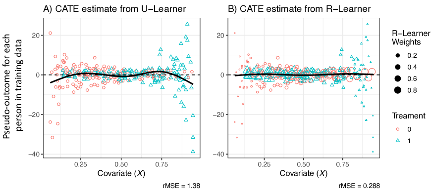
Figure 1: Example of how weights stabilize pseudo-outcome regression, using a single simulated sample. Here, the true conditional average treatment effect is zero for all patients. The estimates from U-Learning & R-Learning are shown as black lines. By down-weighting the observations with high variance, i.e., those with extreme propensity scores, R-Learning is able to achieve a lower rMSE.

1.1.2 Alternative motivation for R-Learner’s weights

As an alternative to Eq (3), a similar motivation for the R-Learner’s weights can be derived by noting that $\left\{A-\hat{\pi}(X)\right\}^{2}$ is roughly proportional the inverse variance of $f_{\text{U,$\hat{\theta}$}}(Z)$ conditional on conditional on $\hat{\theta}$, $X$ and $A$. More specifically, if $Var\left(Y|A,X\right)=\sigma^{2}$ is constant, then

$$Var\left(\frac{Y-\hat{\eta}(X)}{A-\hat{\pi}(X)}|A,X,\hat{\theta}\right)\propto\left\{A-\hat{\pi}(X)\right\}^{-2}.$$

Thus, if we were to expand R-Learning to predict $f_{\text{U,$\hat{\theta}$}}$ as a function of both $X$ and $A$, and if $Var(Y|A,X)$ were constant, then $\left\{A-\hat{\pi}(X)\right\}^{2}$ would form appropriate inverse variance weights, producing the regression problem

$$\arg\min_{\hat{g}}\sum_{i=1}^{n}\left\{A_{i}-\hat{\pi}(X_{i})\right\}^{2}\left\{\frac{Y-\hat{\eta}(X)}{A-\hat{\pi}(X)}-\hat{g}(A_{i},X_{i})\right\}^{2}.$$ (4)

The change to include $A$ as a covariate is balanced by the fact that, if $\hat{\theta}=\theta$, then the population minimizer for Eq (4), $\mathbb{E}\left[\frac{Y-\eta(X)}{A-\pi(X)}|A,X\right]$, does not actually depend on $A$. More specifically, the Robinson Decomposition implies that $\mathbb{E}\left[\frac{Y-\eta(X)}{A-\pi(X)}|A,X\right]=\tau(X)$. Reflecting this fact, if we additionally require the solution to Eq (4) to not depend on $A$, then we recover R-Learning exactly.

1.1.3 Weights in “oracle” R-Learning

A similar connection to stabilizing weights can be seen in the “oracle” version of R-Learning studied by Kennedy (2022a; see their Section 7.6.1). This hypothetical oracle model fits a weighted POR to predict the latent function

$$f_{\text{OR},\theta}(Z) :=\frac{\left\{A-\pi(X)\right\}\left\{Y-\eta(X)\right\}}{\pi(X)\left\{1-\pi(X)\right\}}$$

$$\approx\frac{\left\{A-\hat{\pi}(X)\right\}\left\{Y-\hat{\eta}(X)\right\}}{\left\{A-\hat{\pi}(X)\right\}^{2}}$$

$$=f_{\text{U},\hat{\theta}}(A,X,Y),$$

with weights $\nu(X)=Var(A|X)$. Above, the approximation simply reflects the fact that if $\hat{\pi}=\pi$ then the conditional expectation of the denominators are identical. Again, if the treatment effect is null ($A\perp Y|X$) and the conditional variance of $Y$ is constant (i.e., $Var(Y|X)=\sigma^{2}$), then

$$Var(f_{\text{OR},\theta}(A,X,Y)|X)\propto\nu(X)^{-1}$$

(see Appendix C). Thus, in the null setting, the oracle R-Learner is an inverse-variance weighted POR.

1.1.4 Weights for the DR-Learner

Another pseudo-outcome transformations that can suffer from instability is the “DR-Learner” (Kennedy, 2022a). This method fits a regression using $X$ to predict $f_{\text{DR},\hat{\theta}}(Z)=f_{1,\hat{\theta}}(Z)-f_{0,\hat{\theta}}(Z)$, where

$$f_{a,\hat{\theta}}(Z)$$

$$\hskip 10.00002pt=\hat{\mu}_{a}(X)+\frac{1(A=a)}{a\hat{\pi}(X)+(1-a)\hat{\kappa}(X)}\left(Y-\hat{\mu}_{a}(X)\right).$$ (5)

If $Var(Y|X,A)=\sigma^{2}$ is constant, then it is fairly straightforward to show that $Var\left(f_{\text{DR},\hat{\theta}}(Z)|X,\hat{\theta}=\theta\right)=\kappa(X)^{-1}\pi(X)^{-1}\sigma^{2}$ (Appendix C). Again, extreme values of the propensity score lead to regions where the pseudo-outcome has a high variance. Inspired by this fact, we will see in the sections below that using weights $\hat{\kappa}(X)\hat{\pi}(X)$ when fitting a POR to predict $f_{\text{DR},\hat{\theta}}(Z)$ leads to fast convergence rates and better simulated errors.

Table 1 summarizes the above relationships.

Table 1: Different available pseudo-outcome transformations and their conditional variances given $X$, under certain simplifying assumptions (see Appendix C).

Label	Outcome Transformation	Conditional Variance
U, R ($f_{\text{U},\theta})$	$\frac{Y-\eta(X)}{A-\pi(X)}$	$\propto\frac{\pi^{3}+\left\{1-\pi\right\}^{3}}{\left(1-\pi\right)^{2}\pi^{2}}=\mathbb{E}\left[\left(A-\pi(X)\right)^{-2}|X\right]$
DR ($f_{\text{DR},\theta})$	$\mu_{1}(X)-\mu_{0}(X)\hskip 10.00002pt\hskip 10.00002pt\hskip 10.00002pt\hskip 10.00002pt\hskip 10.00002pt\hskip 10.00002pt$	$\propto 1/\nu(X)$
	$\hskip 10.00002pt\hskip 10.00002pt+\frac{A-\pi(X)}{\pi(X)(1-\pi(X))}\left(Y-\mu_{A}(X)\right)$
Oracle-R $(f_{\text{OR},\theta})$	$\frac{\left\{A-\pi(X)\right\}\left\{Y-\eta(X)\right\}}{\pi(X)(1-\pi(X))}$	$\propto 1/\nu(X)$

2 Simulations

The goal of this simulation section is to examine the role of weights in POR. We include a total of 6 simulation scenarios, labeled A, B, C, D, E & F. The first four are experiments taken from Nie & Wager (2020), with $|X|$ set equal to 10. Setting E is the “low dimensional” simulated example from Kennedy (2022a). Setting F is the simple illustrative example from Figure 1. Table 2 presents each setting in detail, and Table 3 gives a qualitative summary of each setting. The settings generally differ in their complexity for the functions $\eta$, $\tau$ and $\pi$.

Table 2: Simulation Setting Details. Below we show the covariate distribution, CATE function, and nuisance functions for simulations A through F. The notation $\text{trim}_{a}(b)$ is shorthand for $\min(\max(a,b),1-a)$, and the notation $(a)_{+}$ is shorthand for $\max(a,0)$. Settings A-D use multivariate, $iid$ covariates $X$ with a dimension of 10. Here, each element of $X$ follows the distribution shown in the second column. Simulations E & F use univariate $X$. A qualitative description of these simulation settings is shown in Table 3.

Label	$X$ distr.	$\tau\left(x\right)$	$\mathbb{E}\left[Y|X=x\right]$	$\mathbb{E}\left[A|X=x\right]$
A	$U(0,1)$	$\frac{1}{2}x_{1}+\frac{1}{2}x_{2}$	$\sin(\pi x_{1}x_{2})+2\left(x_{3}-\frac{1}{2}\right)^{2}$	$\text{trim}_{0.1}\left\{\sin(\pi x_{1}x_{2})\right\}$
B	$N(0,1)$	$\begin{array}[]{c}\log(1+e^{x_{2}})\\ +x_{1}\end{array}$	$\begin{array}[]{c}\max\{0,x_{1}+x_{2},x_{3}\}\\ \hskip 10.00002pt+\left(x_{4}+x_{5}\right)_{+}\end{array}$	$1/2$
C	$N(0,1)$	1	$2\log\left(1+e^{x_{1}+x_{2}+x_{3}}\right)$	$\frac{1}{1+e^{x_{2}+x_{3}}}$
D	$N(0,1)$	$\begin{array}[]{l}\left(\sum_{i=1}^{3}x_{i}\right)_{+}\\ -\left(x_{4}+x_{5}\right)_{+}\end{array}$	$\begin{array}[]{l}\left(\sum_{i=1}^{3}x_{i}\right)_{+}\\ \hskip 10.00002pt+\frac{1}{2}\left(x_{4}+x_{5}\right)_{+}\end{array}$	$\frac{1}{1+e^{-x_{1}}+e^{-x_{2}}}$
E	$U(-1,1)$	0	$\begin{array}[]{l}1(x_{1}\leq-.5)\frac{(x_{1}+2)^{2}}{2}\\ +1(x_{1}>.5)(x_{1}+0.125)\\ +\left(\frac{x_{1}}{2}+0.875\right)1\left(-\frac{1}{2}<x_{1}<0\right)\\ +\left\{1\left(0<x_{1}<\frac{1}{2}\right)\right.\\ \left.\hskip 10.00002pt\times\left(-5\left(x_{1}-\frac{1}{5}\right)^{2}+1.075)\right)\right\}\end{array}$	$0.1+(0.8x_{1})_{+}$
F	$U\left(\frac{1}{20},\frac{19}{20}\right)$	0	1	$x_{1}$

Table 3: Qualitative summary of the simulation settings detailed in Table 2.

Label	Description	$\tau\left(x\right)$	$\mathbb{E}\left[Y|X=x\right]$	$\mathbb{E}\left[A|X=x\right]$
A	Simple effect	Simple	Complex	Complex
B	Randomized trial	Moderate	Moderate	Constant
C	Complex prognosis	Constant	Complex	Simple
D	Unrelated arms	Moderate	Moderate	Moderate
E	Non-differentiable prognosis	Constant	Complex	Simple
F	Simple illustration	Constant	Constant	Simple

We implemented POR with two pseudo-outcome functions, $f_{U,\hat{\theta}}$ and $f_{\text{DR},\hat{\theta}}$. In each case we used 10-fold cross-fitting. For example, for $f_{U,\hat{\theta}}$, we used 90% of the data to estimate the nuisance functions $\hat{\theta}$, evaluated and stored $f_{U,\hat{\theta}}(Z_{i})$ for the remaining 10%, and then repeated this process 10 times with different fold assignments to obtain a pseudo-outcome for every individual. We then fit a regression against all of these pseudo-outcomes together. We used boosted trees to perform all of our nuisance regressions, as well as the final regression predicting pseudo-outcomes as a function of $X$.

For each pseudo-outcome function, we considered a weighted and unweighted version. For $f_{U,\hat{\theta}}$ we compare uniform weights (i.e., the U-Learner) against weights $\left\{A-\hat{\pi}(X)\right\}^{2}$ (i.e., the R-Learner). For $f_{\text{DR},\hat{\theta}}$ we compare uniform against weights $\hat{\pi}(X)\hat{\kappa}(X)$ (see Table 1).

As a baseline comparator, we consider a “T-Learner” approach (Künzel et al., 2019), which entails separately fitting two estimates $\hat{\mu}_{1}$ and $\hat{\mu}_{0}$ for $\mu_{1}$ and $\mu_{0}$ respectively and then taking $\hat{\mu}_{1}(x_{\text{new}})-\hat{\mu}_{0}(x_{\text{new}})$ as an estimate of $\tau(x_{\text{new}})$. We used the same boosted tree algorithm when fitting the T-Learner.

Figure 2 shows the results of 400 simulation iterations. Weighted POR matched or outperformed unweighted POR in every setting. Performance was similar across the two weighted POR methods we considered. The T-Learner performed comparably to weighted POR in Settings D, E & F, but dramatically underperformed in Settings A, B & C.

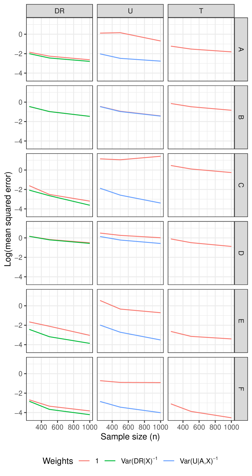
Figure 2: Weighted vs unweighted estimation of simulated CATEs. The columns respectively represent POR with the DR-Learner pseudo-outcome ($f_{\text{DR},\hat{\theta}}$), POR with the U-Learner pseudo-outcome ($f_{\text{U},\hat{\theta}}$), and T-Learning. The rows show the different simulation settings. For the weights, $\text{Var(U|A,X)}^{-1}$ is an abbreviation for $\left\{A-\hat{\pi}(X)\right\}^{2}\propto Var\left(f_{\text{U},\hat{\theta}}(Z)|A,X,\hat{\theta}\right)^{-1}$, and $\text{Var(DR|X)}^{-1}$ is an abbreviation for $\hat{\pi}(X)\hat{\kappa}(X)\approx Var\left(f_{\text{DR},\hat{\theta}}(Z)|X,\hat{\theta}\right)^{-1}$.

3 Convergence Rate Results

Part of the value the IVW framework is that it provides a straightforward path for simplifying expressions for the bias of CATE estimates. Specifically, if $Z,\hat{\kappa},\hat{\pi},$ and $\hat{\mu}$ are mutually independent, we can make use of the following helpful identity.

$$\mathbb{E}\left(\hat{\kappa}\hat{\pi}\left(f_{1,\hat{\theta}}-f_{1,\theta}\right)|X\right)$$

$$\hskip 10.00002pt=\mathbb{E}\left(\hat{\kappa}\hat{\pi}A\left(\frac{1}{\hat{\pi}}-\frac{1}{\pi}\right)(\hat{\mu}_{1}-\mu_{1})|X\right)$$

$$\hskip 10.00002pt=\mathbb{E}\left(\hat{\kappa}\hat{\pi}\pi\left(\frac{1}{\hat{\pi}}-\frac{1}{\pi}\right)(\hat{\mu}_{1}-\mu_{1})|X\right)$$

$$\hskip 10.00002pt=\mathbb{E}\left(\hat{\kappa}|X\right)\mathbb{E}\left(\pi-\hat{\pi}|X\right)\mathbb{E}\left(\hat{\mu}_{1}-\mu_{1}|X\right).$$ (6)

The left-hand side is the weighted conditional bias in estimating $f_{1,\hat{\theta}}$, which we can see depends only on the product of the biases for $\hat{\pi}$ and $\hat{\mu}$. The first equality is shown in Appendix A. The second equality iterates expectations over $\{\hat{\mu}_{1},\hat{\kappa},\hat{\pi}\}$ to replace $A$ with $\pi$. The last comes from the independence assumption. Kennedy (2022a) employs a similar identity when reducing bias terms associated with the oracle R-Learner (see their Section 7.6). In the remainder of this section, Eq (6) will play a fundamental role in our study of convergence rates.

3.1 Notation

Let $\bar{\mathbf{Z}}=(\bar{\mathbf{X}},\bar{\mathbf{a}},\bar{\mathbf{y}})$ denote a dataset of $n$ observations used for POR, which we assume is independent of the data used for estimating the nuisance functions $\hat{\theta}$. Let $d$ denote the dimension of the domain $\mathcal{X}$ of $X$, and let $x_{\text{new}}$ be a point for which we would like to predict $\tau(x_{\text{new}})$.

We will often use the “bar” notation when referring to estimators derived from $\bar{\mathbf{Z}}$; “hat” notation when referring to quantities that depend on nuisance training data; and both notations when referring to estimators derived from both datasets. We do this to help keep track of dependencies between estimated quantities. Let $\mathbf{X}_{\text{all}}$ be the combined matrix of covariates including $\bar{\mathbf{X}}$ as well as the covariates used in training nuisance functions.

Next we introduce notation to describe convergence rates. From random variables $A_{n},B_{n}$, let $A_{n}\lesssim B_{n}$ denote that there exists a constant $c$ such that $A_{n}\leq cB_{n}$ for all $n$. Let $A_{n}\asymp B_{n}$ denote that $A_{n}\lesssim B_{n}$ and $B_{n}\lesssim A_{n}$. Let $A_{n}\lesssim_{\mathbb{P}}c_{n}$ denote that $A_{n}=O_{\mathbb{P}}(c_{n})$ for constants $c_{n}$.

We say that a function $f$ is $s$-smooth if there exists a constant $c$ such that $|f(x)-f_{s,x^{\prime}}(x)|\leq c||x-x^{\prime}||^{s}$ for all $x,x^{\prime}$, where $f_{s,x^{\prime}}$ is the $\lfloor s\rfloor^{th}$ order Taylor approximation of $f$ at $x^{\prime}$. This form of smoothness is a key property of functions in a Hölder class (see, e.g., Tsybakov, 2009; Kennedy, 2022a).

For any function $g(Z)$, let $\bar{\mathbb{P}}_{n}(g(Z)):=\frac{1}{n}\sum_{i=1}^{n}g(Z_{i})$ denote its sample average over $\bar{\mathbf{Z}}$. We frequently omit function arguments when clear from context, writing, for example, $\bar{\mathbb{P}}_{n}(\pi)$ in place of $\bar{\mathbb{P}}_{n}(\pi(X))$.

3.2 Setup & Assumptions

Following Kennedy (2022a), we study convergence rates for an estimator of $\tau$ that uses a local polynomial (LP) regression for the POR step. To define this LP regression, let $h$ be a bandwidth parameter that we expect will shrink with $n$, let kern be a bounded, nonnegative kernel function that is zero outside of the range [-1,1], and let $K(X):=\frac{1}{h^{d}}\texttt{kern}\left(\frac{\|X-x_{\text{new}}\|}{h}\right)$. Let $b$ be a $L$-dimensional, polynomial basis function that is bounded on $\mathcal{X}$. Given independent estimates $\hat{\pi},$ $\hat{\kappa}$ and $\hat{\mu}$, let $\hat{\nu}(X):=\hat{\pi}(X)\hat{\kappa}(X)$, and let $f_{\text{DR},\hat{\theta}}(Z)=f_{1,\hat{\theta}}(Z)-f_{0,\hat{\theta}}(Z)$ be an observed proxy for the transformation $f_{\text{DR},\theta}$, where

$$f_{a,\hat{\theta}}(Z)$$

$$\hskip 10.00002pt=\hat{\mu}_{a}(X)+\frac{1(A=a)}{a\hat{\pi}(X)+(1-a)\hat{\kappa}(X)}\left(Y-\hat{\mu}_{a}(X)\right).$$

Let

$$\hat{\bar{\tau}}(x_{\text{new}}):=\frac{1}{n}\sum_{i=1}^{n}\hat{\bar{w}}(X_{i})f_{\text{DR},\hat{\theta}}(Z_{i})$$

be an estimate of $\tau(x_{\text{new}})$, where

$$\hat{\bar{w}}(x):=b(x_{\text{new}})^{\top}\hat{\bar{\mathbf{Q}}}^{-1}b(x)K(x)\hat{\nu}(x)$$

and

$$\hat{\bar{\mathbf{Q}}}:=\frac{1}{n}\sum_{i=1}^{n}b(X_{i})\hat{\nu}(X_{i})K(X_{i})b(X_{i})^{\top}.$$

Thus, $\hat{\bar{\tau}}(x_{\text{new}})$ is a weighted LP regression predicting $f_{\text{DR},\hat{\theta}}(Z)$ from $X$, with stabilizing weights $\hat{\nu}(X)$. Hereafter, with some abuse of notation, we also use the term “weights” to refer to $\hat{\bar{w}}(X)$.

We study $\hat{\bar{\tau}}(x_{\text{new}})$ by comparing it against an oracle counterpart using the same estimated weights $\hat{\bar{w}}$, but using the true function $f_{\text{DR},\theta}$. That is, we define the oracle estimate

$$\hat{\bar{\tau}}_{\text{oracle}}(x_{\text{new}}):=\frac{1}{n}\sum_{i=1}^{n}\hat{\bar{w}}(X_{i})f_{\text{DR},\theta}(Z_{i}).$$

Given $\hat{\pi}$ and $\hat{\kappa}$, this oracle estimate is a weighted LP regression predicting $f_{\text{DR},\theta}(Z)$ from $X$, evaluated at the point $X=x_{\text{new}}$.

Next, we present several assumptions. We reuse the notation “$c$” to refer to generic constants; the same constant need not satisfy all assumptions.

Assumption 3.1.

(Regularity) $\mathbb{E}\left(Y^{2}|A,X\right)$ is bounded.

Assumption 3.2.

(Positivity) There exists a constant $c\in(0,1)$ such that, for all covariate values $x$, all $a\in\{0,1\}$, and all sample sizes $n$, we have $c\leq\hat{\kappa}(x),\kappa(x),\hat{\pi}(x),\pi(x)<1-c$.

Assumption 3.3.

(Nuisance Error) There exists a complexity parameter $k$ (e.g., the number of parameters a model) and constants $c$, $s_{\mu}$ and $s_{\pi}$, such that, with probability approaching 1, the sequences $\mathsf{V}_{k,n}:=ck/n$, $\mathsf{B}_{\pi,k}:=ck^{-s_{\pi}/d}$ and $\mathsf{B}_{\mu,k}:=ck^{-s_{\mu}/d}$ satisfy

$$Var(\hat{\pi}(x)|\mathbf{X}_{\text{all}}) \leq\mathsf{V}_{k,n},$$

$$Var(\hat{\kappa}(x)|\mathbf{X}_{\text{all}}) \leq\mathsf{V}_{k,n},$$

$$Var(\hat{\mu}_{a}(x)|\mathbf{X}_{\text{all}}) \leq\mathsf{V}_{k,n},$$

and

$$\mathbb{E}(\hat{\pi}(x)-\pi(x)|\mathbf{X}_{\text{all}}) \leq\mathsf{B}_{\pi,k},$$

$$\mathbb{E}(\hat{\kappa}(x)-\kappa(x)|\mathbf{X}_{\text{all}}) \leq\mathsf{B}_{\pi,k},$$

$$\mathbb{E}(\hat{\mu}_{a}(x)-\mu_{a}(x)|\mathbf{X}_{\text{all}}) \leq\mathsf{B}_{\mu,k}$$

for all $x$ and $a$. Above, we assume that $k$ grows with $n$, and that $k<n$.

The bias conditions of Assumption 3.3 will typically require $\mu_{a}$ and $\pi$ to be $s_{\mu}$-smooth and $s_{\pi}$-smooth respectively. The variance conditions typically will require the complexity of the nuisance models (i.e., $k$) to grow at a limited rate. For example, for spline estimators, they generally require the design matrices to have stable eigenvalues with high probability. This can be ensured by requiring $k\log(k)/n$ to converge zero (see, e.g., Tropp, 2015; Belloni et al., 2015; Newey & Robins, 2018).

Assumption 3.4.

(Limited bandwidth) $n>1/h^{d}$.

Assumption 3.4 is fairly minimal, and is made for simplicity of presentation. Roughly speaking, it says that $n$ needs to be at least as large as the number of $h$-diameter subregions required to fully partition the covariate space.

Assumption 3.5.

(Eigenvalue Stability) There exists a constant $c>0$ such that $\lambda_{\min}\left(\hat{\bar{\mathbf{Q}}}\right)>c$ with probability approaching 1.

Assumption 3.5 ensures that the weights $\hat{\bar{w}}$ are bounded in probability. Kennedy (2022a) makes a similar assumption in their Theorem 3.

Assumption 3.6.

($X$ Distribution) The density of $X$ is approximately uniform in the sense that, for any $h>0$ and $x\in\mathcal{X}$, we have $\text{Pr}\left[\|X-x\|\leq h\right]\lesssim h^{d}$.

Assumption 3.7.

(Local Nuisance Estimators) There exists a constant $c$ such that $Cov(\hat{\pi}(x),\hat{\pi}(x^{\prime}))=0$, $Cov(\hat{\kappa}(x),\hat{\kappa}(x^{\prime}))=0$, and $Cov(\hat{\mu}_{a}(x),\hat{\mu}_{a}(x^{\prime}))=0$ for all $x,x^{\prime},a$ satisfying $\|x-x^{\prime}\|>ck^{-1/d}$.

Assumption 3.7 says that the nuisance models’ predictions for sufficiently far away points $x,x^{\prime}$ depend on entirely different training data. This is true, for example, in $r$-order spline regression models that divide each dimension into $p$ partitions, producing a total of $p^{d}$ neighborhoods and $k=p^{d}d^{r}$ parameters. If the neighborhoods are approximately evenly sized and $\mathcal{X}$ is the unit hypercube, the maximum distance within a neighborhood is $\left(\sum_{i=1}^{d}1/p^{2}\right)^{1/2}=d^{1/2}/p=d^{1/2+r/d}k^{-1/d},$ where the last equality comes from rearranging $k=p^{d}d^{r}$. Thus, predictions for points $x,x^{\prime}$ that are at least $d^{1/2+r/d}k^{-1/d}$ apart will be independent, as they are created from different neighborhoods of training data.

3.3 Convergence rate results

The assumptions in the previous section allow us to characterize the difference between $\hat{\bar{\tau}}(x_{\text{new}})$ and the oracle estimate.

Theorem 3.8.

(Error with respect to oracle) Under Assumptions 3.1-3.7, we have the following results.

1. (4-way CF) If $\hat{\pi},\hat{\kappa},\hat{\mu}$, and $\bar{\mathbf{Z}}$ are mutually independent, then

   $$\hat{\bar{\tau}}(x_{\text{new}})-\hat{\bar{\tau}}_{\text{oracle}}(x_{\text{new}})\lesssim_{\mathbb{P}}\sqrt{\frac{1}{nh^{d}}}+\mathsf{B}_{\mu}\mathsf{B}_{\pi}.\hphantom{+\frac{k^{1/2-s_{\mu}/d}}{n}+\frac{k^{1/2-s_{\pi}/d}}{n}+\frac{k}{n}}$$

2. (3-way CF) If $\hat{\pi},\hat{\mu}$ and $\bar{\mathbf{Z}}$ are mutually independent; $\hat{\kappa}(x)=1-\hat{\pi}(x)$; and
   Var$\left[\sup_{x}\left\{\hat{\pi}(x)-\pi(x)\right\}^{2}|\mathbf{X}_{\text{all}}\right]\lesssim k_{n}/n$ with probability approaching 1, then

   $$\hat{\bar{\tau}}(x_{\text{new}})-\hat{\bar{\tau}}_{\text{oracle}}(x_{\text{new}})\lesssim_{\mathbb{P}}\sqrt{\frac{1}{nh^{d}}}+\mathsf{B}_{\mu}\left(\mathsf{B}_{\pi}+\mathsf{V}_{k,n}\right).\hphantom{+\frac{k^{1/2/2-s_{\pi}/d}}{n}+\frac{k}{n}}$$

3. (2-way CF) If $\{\hat{\pi},\hat{\mu}\}\perp\bar{\mathbf{Z}}$ and $\hat{\kappa}(x)=1-\hat{\pi}(x)$, then

   $$\hat{\bar{\tau}}(x_{\text{new}})-\hat{\bar{\tau}}_{\text{oracle}}(x_{\text{new}})$$

   $$\hskip 10.00002pt\lesssim_{\mathbb{P}}\sqrt{\frac{1}{nh^{d}}}+\left(\mathsf{B}_{\mu}+\sqrt{\mathsf{V}_{k,n}}\right)\left(\mathsf{B}_{\pi}+\sqrt{\mathsf{V}_{k,n}}\right).$$

The three bounds given by Theorem 3.8 become less powerful as we relax the independence assumptions. As in Newey & Robins (2018) and Kennedy (2022a), the independence conditions can be ensured via higher-order cross-fitting, or “nested” cross-fitting, in which separate folds are used to estimate each nuisance function. Higher order cross-fitting is typically impractical in small or moderate sample sizes, as it requires that a smaller fraction of data points be used to train each nuisance function. That said, the effect of dividing our sample into smaller partitions will be asymptotically dwarfed by the effect of a faster convergence rate.

Point 3 makes the weakest assumptions and produces the least powerful bound. It is similar to the bound in Lemma 2 of Nie & Wager, 2020. That is, Point 3 implies that $\hat{\bar{\tau}}(x_{\text{new}})-\hat{\bar{\tau}}_{\text{oracle}}(x_{\text{new}})\lesssim_{\mathbb{P}}1/\sqrt{nh^{d}}$ if the conditional rMSE of $\hat{\pi}(x)$ and $\hat{\mu}_{a}(x)$ are $\lesssim n^{-1/4}$. The $\sqrt{1/nh^{d}}$ term common to all three bounds is a standard variance term associated with LP regression (see, e.g., Proposition 1.13 of Tsybakov, 2009, or Theorem 3 of Kennedy, 2022a). The variance condition in Point 2 is similar to Assumption 3.3, and we expect it to hold in similar situations.

To bound the error of the oracle itself, we additionally assume the following.

Assumption 3.9.

The target function $\tau$ is $s_{\tau}$-smooth, and the basis $b$ is of order at least $\lfloor s_{\tau}\rfloor$.

From here, fairly standard results for local polynomial regression (e.g., Tsybakov, 2009; see also Kennedy, 2022a) imply the following result.

Theorem 3.10.

(Oracle error) Under Assumptions 3.1-3.7 and Assumption 3.9,

$$\hat{\bar{\tau}}_{\text{oracle}}(x_{\text{new}})-\tau(x_{\text{new}})\lesssim_{\mathbb{P}}\sqrt{\frac{1}{nh^{d}}}+h^{s_{\tau}}.$$

Combining the results of Theorems 3.8 & 3.10, we see that

$$\hat{\bar{\tau}}(x_{\text{new}})-\tau(x_{\text{new}})\lesssim_{\mathbb{P}}\sqrt{\frac{1}{nh^{d}}}+h^{s_{\tau}}+\mathsf{B}_{\mu}\mathsf{B}_{\pi}$$ (7)

when $\hat{\pi},\hat{\kappa},\hat{\mu}$ and $\bar{\mathbf{Z}}$ are mutually independent and Assumptions 3.1-3.7 and 3.9 hold.

The bound in Eq (7) is at least as low as the bound established by Kennedy (2022a), which adds an additional $\mathsf{B}_{\pi}^{2}$ term. Our bound is not as low as the minimax bound established by Kennedy et al. (2022), although the latter depends on a slightly stronger assumption. Roughly speaking, Kennedy et al. assume approximate knowledge of the covariate distribution, which replaces our need for the covariance estimator $\hat{\bar{\mathbf{Q}}}$ and allows the authors to replace our $\mathsf{B}_{\mu}\mathsf{B}_{\pi}$ term with $\mathsf{B}_{\mu}\mathsf{B}_{\pi}h^{s_{\mu}+s_{\pi}}$ (2022; see their Eq (16)).

4 Discussion

We have argued that R-Learning implicitly employs a POR with stabilizing weights, and that these weight are key to its success. We also consider doubly robust estimators that incorporate IVW more directly, and show that they can attain a convergence rate that is, to our knowledge, the fastest available under our minimal assumptions (Eq (7)).

The use of weighted regression highlights two fundamental differences in the difficulty of estimating the CATE versus the ATE. The CATE is harder to estimate than the ATE in the sense that it is inherently a more complex target, and so it incurs a higher oracle error. Indeed, if the underlying CATE function is sufficiently non-smooth, then the oracle error erodes any advantage of using doubly robust methods over plug-in (“T-Learner”) methods. However, roughly speaking, when estimating the CATE we have the extra advantage of being able to use IVW without inducing confounding bias, and so the (higher) oracle error rate becomes easier to attain. Both differences disappear in the homogeneous effect setting when the CATE is constant, in which case IVW is a natural approach for improving the ATE estimate (see, e.g., Hullsiek & Louis, 2002; Yao et al., 2021).

Our work also highlights an important caveat for R-Learning, which is that it requires all confounders to be used as inputs in any resulting decision support tool. For example, consider the process of applying R-Learning to observational study in order to build a tool to identify patients who will benefit most from a treatment. Doctors using this tool must have access to all variables $(X)$ that were used for confounding adjustment in the study. If the study involved extensive lab tests, then this requirement may not be feasible. Alternatively, if the study adjusted for race and income, in addition to insurance status, then doctors may face ethical concerns if they allow information about a patient’s race or income to influence their recommended treatments. While this problem can be partially mitigated by fitting an additional regression to predict the R-Learning estimate from a subset of allowed decision factors $V$, R-Learning may still underperform due to the fact that it internally estimates a target that is more complex than is necessary. Here, approaches that directly estimate the coarsened function $\mathbb{E}\left(\tau(X)|V\right)$ may improve accuracy due to the low oracle error associated with estimating lower-dimensional functions (see, e.g., Fisher & Fisher, 2023).

Appendix A Proof of Theorem 3.8

Throughout the appendix, we will sometimes use colored text when writing long equations to flag parts of an equation that change from one line to the next (e.g., Line (8)). We use I.E. as an abbreviation for “iterating expectations.”

Proof.

Throughout the sections below we will use the fact if $1_{n}A_{n}\lesssim_{\mathbb{P}}b_{n}$ and $1_{n}$ is an indicator satisfying $\text{Pr}(1_{n}=1)\rightarrow 1$ (at any rate), then $A_{n}\lesssim_{\mathbb{P}}b_{n}$ as well. In particular, we define $\hat{\bar{1}}$ to be the event that the inequalities in Assumptions 3.3 and 3.5 hold. By these same assumptions, $\text{Pr}(\hat{\bar{1}}=1)\rightarrow 1$. When attempting to bound any given term $A_{n}$ in probability, it will be sufficient to bound $\hat{\bar{1}}A_{n}$.

We can now present a proof outline. First, we decompose the error with respect to the oracle as

$$\hat{\bar{\tau}}(x_{\text{new}})-\hat{\bar{\tau}}_{\text{oracle}}(x_{\text{new}}) =\bar{\mathbb{P}}_{n}\left\{\hat{\bar{w}}\left(\left(f_{1,\hat{\theta}}-f_{0,\hat{\theta}}\right)-\left(f_{1,\theta}-f_{0,\theta}\right)\right)\right\}$$

$$=\bar{\mathbb{P}}_{n}\left\{\hat{\bar{w}}\left(f_{1,\hat{\theta}}-f_{1,\theta}\right)\right\}-\bar{\mathbb{P}}_{n}\left\{\hat{\bar{w}}\left(f_{0,\hat{\theta}}-f_{0,\theta}\right)\right\}.$$

Due to the symmetry of the problem, proving that either one of the above terms is bounded will be sufficient. Without loss of generality (WLOG), we focus on the first term. After multiplying by $\hat{\bar{1}}$, which does not change the bound, we have

$$\hat{\bar{1}}\bar{\mathbb{P}}_{n}\left\{\hat{\bar{w}}\left(f_{1,\hat{\theta}}-f_{1,\theta}\right)\right\} =\hat{\bar{1}}\bar{\mathbb{P}}_{n}\left[\hat{\bar{w}}\left\{\hat{\mu}_{1}-\mu_{1}+\frac{A}{\hat{\pi}}\left(Y-\hat{\mu}_{1}\right)-\frac{A}{\pi}\left(Y-\mu_{1}\right)\right\}\right]$$

$$=\hat{\bar{1}}\bar{\mathbb{P}}_{n}\left[\hat{\bar{w}}\left\{\hat{\mu}_{1}-\mu_{1}{\color[rgb]{.75,0,.25}-\frac{A}{\pi}\hat{\mu}_{1}}+{\color[rgb]{0,0,1}\frac{A}{\pi}\mu_{1}}\right.\right.$$

$$\hskip 10.00002pt\hskip 10.00002pt+\frac{A}{\hat{\pi}}Y{\color[rgb]{1,0,0}-\frac{A}{\hat{\pi}}\mu_{1}}-\frac{A}{\pi}Y+\frac{A}{\pi}\mu_{1}$$

$$\hskip 10.00002pt\hskip 10.00002pt\left.\left.-\frac{A}{\hat{\pi}}\hat{\mu}_{1}{\color[rgb]{1,0,0}+\frac{A}{\hat{\pi}}\mu_{1}}{\color[rgb]{.75,0,.25}+\frac{A}{\pi}\hat{\mu}_{1}}-{\color[rgb]{0,0,1}\frac{A}{\pi}\mu_{1}}\right\}\right]$$ (8)

$$=\hat{\bar{1}}\bar{\mathbb{P}}_{n}\left[\hat{\bar{w}}\left(1-\frac{A}{\pi}\right)(\hat{\mu}_{1}-\mu_{1})\right]$$ (9)

$$\hskip 10.00002pt\hskip 10.00002pt+\hat{\bar{1}}\bar{\mathbb{P}}_{n}\left[\hat{\bar{w}}A\left(\frac{1}{\hat{\pi}}-\frac{1}{\pi}\right)(Y-\mu_{1})\right]$$ (10)

$$\hskip 10.00002pt\hskip 10.00002pt-\hat{\bar{1}}\bar{\mathbb{P}}_{n}\left[\hat{\bar{w}}A\left(\frac{1}{\hat{\pi}}-\frac{1}{\pi}\right)(\hat{\mu}_{1}-\mu_{1})\right].$$ (11)

Section A.1, below, shows that the weights $\hat{\bar{w}}$ satisfy $\mathbb{E}\left(\hat{\bar{1}}\hat{\bar{w}}(X_{i})^{2}\right)\lesssim 1/h^{d}$ (as in Kennedy (2022a)’s Lemma 1). Under the condition that $(\hat{\pi},\hat{\kappa},\hat{\mu}_{1})\perp\bar{\mathbf{Z}}$, Section A.2 shows that Lines (9) & (10) are weighted averages of terms that are $iid$ and mean zero, conditional $\hat{\pi},\hat{\kappa},\hat{\mu}_{1}$ and $\bar{\mathbf{X}}_{\text{all}}$. It will follow that Lines (9) & (10) have expected conditional variance bounded by $1/\left(nh^{d}\right)$. Thus, Lines (9) & (10) are

$$\lesssim_{\mathbb{P}}\frac{1}{\sqrt{nh^{d}}}$$ (12)

by Markov’s Inequality (see Section A.2 for details). This fact holds for all forms of independence considered in Theorem 3.8 (Points 1, 2 & 3), as it depends only on $(\hat{\pi},\hat{\kappa},\hat{\mu}_{1})\perp\bar{\mathbf{Z}}$. As an aside, these same steps can be used to show the first equality in Eq (6).

Line (11) does not have mean zero given $\hat{\pi},\hat{\kappa},\hat{\mu}_{1}$ and $\bar{\mathbf{X}}_{\text{all}}$, and so constitutes the bias relative to the oracle. These terms are more challenging to tackle due to the correlations between the $\hat{\bar{\mathbf{Q}}}$ matrix (contained within $\hat{\bar{w}}$) and the $1/\hat{\pi}$ nuisance estimate. However, we can separate these quantities using the Cauchy Schwartz inequality. Line (11) becomes

$$\hat{\bar{1}}\bar{\mathbb{P}}_{n}\left\{\hat{\bar{w}}A\left(\frac{1}{\hat{\pi}}-\frac{1}{\pi}\right)(\hat{\mu}_{1}-\mu_{1})\right\}$$

$$\hskip 10.00002pt\hskip 10.00002pt=\hat{\bar{1}}b(x_{\text{new}})^{\top}\hat{\bar{\mathbf{Q}}}^{-1}\bar{\mathbb{P}}_{n}\left\{b(X_{i})K(X_{i})\hat{\nu}(X_{i})A_{i}\left(\frac{1}{\hat{\pi}}-\frac{1}{\pi}\right)(\hat{\mu}_{1}-\mu_{1})\right\} \text{def of }\hat{\bar{w}}$$

$$\hskip 10.00002pt\hskip 10.00002pt\leq\hat{\bar{1}}\left\|\hat{\bar{\mathbf{Q}}}^{-1}b(x_{\text{new}})\right\|\;\left\|\bar{\mathbb{P}}_{n}\left\{bK\hat{\nu}A\left(\hat{\pi}^{-1}-\pi^{-1}\right)(\hat{\mu}_{1}-\mu_{1})\right\}\right\|$$ Cauchy Schwartz

$$\hskip 10.00002pt\hskip 10.00002pt\lesssim\hat{\bar{1}}\left\|\bar{\mathbb{P}}_{n}\left\{bK\hat{\nu}A\left(\hat{\pi}^{-1}-\pi^{-1}\right)(\hat{\mu}_{1}-\mu_{1})\right\}\right\| \text{def of }\hat{\bar{1}}\text{ \& }b$$

$$\hskip 10.00002pt\hskip 10.00002pt=\left[\sum_{l=1}^{L}\hat{\bar{1}}\bar{\mathbb{P}}_{n}\left\{b_{\ell}K\hat{\nu}A\left(\hat{\pi}^{-1}-\pi^{-1}\right)(\hat{\mu}_{1}-\mu_{1})\right\}^{2}\right]^{1/2}$$

$$\hskip 10.00002pt\hskip 10.00002pt\leq\sum_{l=1}^{L}\left|\hat{\bar{1}}\bar{\mathbb{P}}_{n}\left\{b_{\ell}K\hat{\kappa}\hat{\pi}A\left(\hat{\pi}^{-1}-\pi^{-1}\right)(\hat{\mu}_{1}-\mu_{1})\right\}\right|,$$ (13)

where the last $\leq$ comes from the definition of $\hat{\nu},$ and from the fact that $\sum_{j=1}^{J}a_{j}^{2}\leq\left(\sum_{j=1}^{J}a_{j}\right)^{2}$ for any nonnegative sequences of values $\{a_{j},\dots,a_{J}\}$.

Appealing to Markov’s Inequality, we tackle Line (13) by bounding the second moment of each summand. For Point 1, we use the fact that $\mathbb{E}(V^{2})=Var(V)+\mathbb{E}(V)^{2}$ for any random variable $V$ to bound

$$\mathbb{E}\left[\mathbb{E}\left\{\hat{\bar{1}}\bar{\mathbb{P}}_{n}\left\{b_{\ell}K\hat{\kappa}\hat{\pi}A\left(\hat{\pi}^{-1}-\pi^{-1}\right)(\hat{\mu}_{1}-\mu_{1})\right\}^{2}|\mathbf{X}_{\text{all}},\hat{\kappa}\right\}\right]$$

$$\;\;=\mathbb{E}\left[\mathbb{E}\left\{\hat{\bar{1}}\bar{\mathbb{P}}_{n}\left\{b_{\ell}K\hat{\kappa}\hat{\pi}A\left(\hat{\pi}^{-1}-\pi^{-1}\right)(\hat{\mu}_{1}-\mu_{1})\right\}|\mathbf{X}_{\text{all}},\hat{\kappa}\right\}^{2}\right]$$ (14)

$$\;\;\;\;\;\;+\mathbb{E}\left[Var\left\{\hat{\bar{1}}\bar{\mathbb{P}}_{n}\left\{b_{\ell}K\hat{\kappa}\hat{\pi}A\left(\hat{\pi}^{-1}-\pi^{-1}\right)(\hat{\mu}_{1}-\mu_{1})\right\}|\mathbf{X}_{\text{all}},\hat{\kappa}\right\}\right]$$ (15)

Section A.3 shows that Line (14) is

$$\lesssim k^{-2(s_{\mu}+s_{\pi})/d}$$

when $\hat{\pi}\perp\hat{\kappa}$, using steps similar to those in Eq (6).

Section A.4 shows that Line (15) is $\lesssim 1/\left(nh^{d}\right)$. Thus, Eq (13) is

$$\lesssim_{\mathbb{P}}\sqrt{\frac{1}{nh^{d}}}+k^{-(s_{\mu}+s_{\pi})/d}.$$

This, combined with Line (12), completes the proof of Point 1.

Section A.5 shows that Line (13) is

$$\lesssim_{\mathbb{P}}k^{-(s_{\mu}-s_{\pi})/d}+\frac{k^{1-s_{\mu}/d}}{n}+\sqrt{\frac{1}{nh^{d}}}$$

under the conditions of Point 2, and Section A.6 shows that Line (13) is

$$\lesssim_{\mathbb{P}}\frac{k}{n}+\frac{k^{1/2-s_{\mu}/d}}{\sqrt{n}}+\frac{k^{1/2-s_{\pi}/d}}{\sqrt{n}}+k^{-\left(s_{\mu}+s_{\pi}\right)/d}$$

under the conditions of Point 3. This completes the proof for Points 2 & 3. ∎

A.1 Bound on weights

Here we show results for the weights $\hat{\bar{w}}$. Our approach closely follows classic approaches for LP regression (e.g., Tsybakov, 2009; see also Kennedy, 2022a). Let $\mathcal{I}(x)=1(\|x-x_{\text{new}}\|\leq h)$, so that $K(x)=0$ and $\hat{\bar{w}}(x)=0$ whenever $\mathcal{I}(x)=0$ by the definitions of $K$ and $\hat{\bar{w}}$.

Lemma A.1.

(Bounded weights) Under Assumptions 3.4, 3.5 & 3.6:

1. $K(X)\lesssim\frac{1}{h^{d}}\mathcal{I}(X)$, and $\mathbb{E}\left(|K(X)|\right)\lesssim\frac{1}{h^{d}}\mathbb{E}\left(\mathcal{I}(X)\right)\lesssim 1$;

2. $\mathbb{E}\left[\left\{\frac{1}{n}\sum_{i=1}^{n}|K(X_{i})|\right\}^{2}\right]\lesssim 1$;

3. $\hat{\bar{1}}|\hat{\bar{w}}(x)|\lesssim\mathcal{I}(x)/h^{d}$ for any fixed $x$;

4. $\mathbb{E}\left\{\hat{\bar{1}}|\hat{\bar{w}}(X_{i})|\right\}\lesssim 1$; and

5. $\mathbb{E}\left\{\hat{\bar{1}}\hat{\bar{w}}(X_{i})^{2}\right\}\lesssim 1/h^{d}$.

Proof.

Point 1 comes immediately from the definitions of $K$ and $\mathcal{I}$, and from Assumption 3.6.

For Point 2,

$$\mathbb{E}\left[\left\{\frac{1}{n}\sum_{i=1}^{n}|K(X_{i})|\right\}^{2}\right] \lesssim\frac{1}{n^{2}h^{2d}}\mathbb{E}\left[\left\{\sum_{i=1}^{n}\mathcal{I}(X_{i})\right\}^{2}\right]$$ Point 1

$$=\frac{1}{n^{2}h^{2d}}\left[\mathbb{E}\left\{\sum_{i=1}^{n}\mathcal{I}(X_{i})\right\}+\mathbb{E}\left\{\sum_{i=1}^{n}\mathcal{I}(X_{i})\sum_{j\neq i}^{n}\mathbb{E}\left(\mathcal{I}(X_{j})|X_{i}\right)\right\}\right]$$

$$\lesssim\frac{1}{n^{2}h^{2d}}\left[nh^{d}+n(n-1)h^{2d}\right]$$ Assm 3.6

$$=\frac{1}{nh^{d}}+\frac{1}{n^{2}}\left[n(n-1)\right]$$

$$\leq 1.$$ Assm 3.4.

For Point 3,

$$\hat{\bar{1}}|\hat{\bar{w}}(x)| \leq\hat{\bar{1}}\|b(x_{\text{new}})\|\;\|\hat{\bar{\mathbf{Q}}}^{-1}b(x)K(x)\hat{\pi}(x)\|$$ Cauchy Schwartz

$$\lesssim\hat{\bar{1}}\|\hat{\bar{\mathbf{Q}}}^{-1}b(x)K(x)\hat{\nu}(x)\| \text{def of }b$$

$$\leq\frac{\hat{\bar{1}}}{\lambda_{\min}\left(\hat{\bar{\mathbf{Q}}}\right)}\|b(x)K(x)\hat{\nu}(x)\|$$

$$\lesssim\|b(x)K(x)\hat{\nu}(x)\| \text{def of }\hat{\bar{1}}$$

$$\leq|K(x)| \text{def of }b,\text{Assm \ref{assu:positivity}}$$

$$\lesssim\frac{1}{h^{d}}\mathcal{I}(x)$$ Point 1.

Point 4 follows from Points 1 & 3. Similarly, for Point 5,

$$\mathbb{E}\left\{\hat{\bar{1}}\hat{\bar{w}}(X_{i})^{2}\right\}\lesssim\frac{1}{h^{2d}}\mathbb{E}\left\{\mathcal{I}(x)\right\}\lesssim\frac{1}{h^{d}},$$

where the first $\lesssim$ is from Point 3 and the second is from Assumption 3.6. ∎

A.2 Showing Lines (9) & (10) are $\lesssim_{\mathbb{P}}\sqrt{1/(nh^{d})}$

Line (9) has conditional expectation

$$\hat{\bar{1}}\mathbb{E}\left[\bar{\mathbb{P}}_{n}\left(\hat{\bar{w}}\left(1-\frac{A}{\pi}\right)(\hat{\mu}_{1}-\mu_{1})\right)|\bar{\mathbf{X}}_{\text{all}},\hat{\mu}_{1},\hat{\pi},\hat{\kappa}\right]$$

$$=\hat{\bar{1}}\bar{\mathbb{P}}_{n}\left(\hat{\bar{w}}\left(1-\frac{{\color[rgb]{.75,0,.25}\pi}}{\pi}\right)(\hat{\mu}_{1}-\mu_{1})\right)$$

$$=0$$

and conditional variance

$$\hat{\bar{1}}Var\left[\bar{\mathbb{P}}_{n}\left(\hat{\bar{w}}\left(1-\frac{A}{\pi}\right)(\hat{\mu}_{1}-\mu_{1})\right)|\bar{\mathbf{X}}_{\text{all}},\hat{\mu}_{1},\hat{\pi},\hat{\kappa}\right]$$

$$\hskip 10.00002pt=\frac{\hat{\bar{1}}}{n^{2}}\sum_{i=1}^{n}\hat{\bar{w}}(X_{i})^{2}(\hat{\mu}_{1}(X_{i})-\mu_{1}(X_{i}))^{2}\frac{1}{\pi(X_{i})^{2}}Var\left[A|\bar{\mathbf{X}}_{\text{all}}\right]$$

$$\hskip 10.00002pt\lesssim\frac{\hat{\bar{1}}}{n^{2}}\sum_{i=1}^{n}\hat{\bar{w}}(X_{i})^{2}(\hat{\mu}_{1}(X_{i})-\mu_{1}(X_{i}))^{2}$$ Assm 3.2

$$\hskip 10.00002pt\lesssim_{\mathbb{P}}\frac{1}{n^{2}}\sum_{i=1}^{n}\mathbb{E}\left[\hat{\bar{1}}\hat{\bar{w}}(X_{i})^{2}\mathbb{E}\left\{(\hat{\mu}_{1}(X_{i})-\mu_{1}(X_{i}))^{2}|\mathbf{X}_{\text{all}}\right\}\right]$$ Markov’s Ineq

$$\hskip 10.00002pt\lesssim\frac{1}{n^{2}}\sum_{i=1}^{n}\mathbb{E}\left[\hat{\bar{1}}\hat{\bar{w}}(X_{i})^{2}\right] \text{def of }\hat{\bar{1}}$$

$$\hskip 10.00002pt\lesssim\frac{1}{nh^{d}}.$$ Lemma A.1.5.

Combining this with the fact that Line (9) is mean zero given $\bar{\mathbf{X}}_{\text{all}},\hat{\mu}_{1},\hat{\pi}$, and $\hat{\kappa}$ we have

$$\hat{\bar{1}}\mathbb{E}\left[\bar{\mathbb{P}}_{n}\left(\hat{\bar{w}}\left(1-\frac{A}{\pi}\right)(\hat{\mu}_{1}-\mu_{1})\right)^{2}|\bar{\mathbf{X}}_{\text{all}},\hat{\mu}_{1},\hat{\pi},\hat{\kappa}\right]$$

$$=\hat{\bar{1}}Var\left[\bar{\mathbb{P}}_{n}\left(\hat{\bar{w}}\left(1-\frac{A}{\pi}\right)(\hat{\mu}_{1}-\mu_{1})\right)^{2}|\bar{\mathbf{X}}_{\text{all}},\hat{\mu}_{1},\hat{\pi},\hat{\kappa}\right]$$

$$\lesssim_{\mathbb{P}}\frac{1}{nh^{d}},$$

which implies that Line (9) is $\lesssim_{\mathbb{P}}\sqrt{\frac{1}{nh^{d}}}$ by Markov’s Inequality (see Lemma 2 of Kennedy, 2022a for details).

Similarly, Line (10) has conditional expectation

$$\mathbb{E}\left[\bar{\mathbb{P}}_{n}\left(\hat{\bar{w}}A\left(\frac{1}{\hat{\pi}}-\frac{1}{\pi}\right)(Y-\mu_{1})\right)|\bar{\mathbf{X}}_{\text{all}},\hat{\mu}_{1},\hat{\pi},\hat{\kappa}\right]$$

$$=\bar{\mathbb{P}}_{n}\left[\hat{\bar{w}}\left(\frac{1}{\hat{\pi}}-\frac{1}{\pi}\right)\mathbb{E}\left\{A(Y-\mu_{1})|X\right\}\right]$$

$$=\bar{\mathbb{P}}_{n}\left[\hat{\bar{w}}\left(\frac{1}{\hat{\pi}}-\frac{1}{\pi}\right)\mathbb{E}\left\{Y-\mu_{1}|X,A=1\right\}\pi(X)\right]$$

$$=0.$$ (16)

and conditional variance

$$Var\left[\bar{\mathbb{P}}_{n}\left(\hat{\bar{w}}A\left(\frac{1}{\hat{\pi}}-\frac{1}{\pi}\right)(Y-\mu_{1})\right)|\bar{\mathbf{X}}_{\text{all}},\hat{\mu}_{1},\hat{\pi},\hat{\kappa}\right]$$

$$\hskip 10.00002pt=\frac{1}{n^{2}}\sum_{i=1}^{n}\hat{\bar{w}}(X_{i})^{2}\left(\frac{1}{\hat{\pi}(X_{i})}-\frac{1}{\pi(X_{i})}\right)^{2}Var\left[A(Y-\mu_{1})|\bar{\mathbf{X}}_{\text{all}}\right]$$

$$\hskip 10.00002pt\lesssim\frac{1}{n^{2}}\sum_{i=1}^{n}\hat{\bar{w}}(X_{i})^{2}$$ Assms 3.1 & 3.2

$$\hskip 10.00002pt\lesssim_{\mathbb{P}}\frac{1}{nh^{d}}$$ Lemma A.1.5 + Markov’s Ineq.

Thus, the same reasoning implies that Line (10) is $\lesssim_{\mathbb{P}}\sqrt{\frac{1}{nh^{d}}}$.

A.3 Showing Line (14) is $\lesssim k^{-2\left(s_{\mu}+s_{\pi}\right)}$ when $\hat{\pi}\perp\hat{\kappa}$

Let $\hat{1}$ be the indicator that the inequalities in Assumption 3.3 hold, where $\hat{1}\geq\hat{\bar{1}}$, and $\hat{1}$ depends only on $\mathbf{X}_{\text{all}}$. The inner expectation in Line (14) equals

$$\mathbb{E}\left[\hat{\bar{1}}\bar{\mathbb{P}}_{n}\left\{b_{\ell}K\hat{\kappa}\hat{\pi}A\left(\hat{\pi}^{-1}-\pi^{-1}\right)(\hat{\mu}_{1}-\mu_{1})\right\}|\mathbf{X}_{\text{all}},\hat{\kappa}\right]$$

$$\leq\frac{{\color[rgb]{0,0,1}\hat{1}}}{n}\sum_{i=1}^{n}b_{\ell}(X_{i})K(X_{i})\hat{\kappa}(X_{i})$$

$$\hskip 10.00002pt\hskip 10.00002pt\hskip 10.00002pt\times\mathbb{E}\left[A\left(1-\frac{\hat{\pi}(X_{i})}{\pi(X_{i})}\right)|\mathbf{X}_{\text{all}}\right]\mathbb{E}\left[\hat{\mu}_{1}(X_{i})-\mu_{1}(X_{i})|\mathbf{X}_{\text{all}}\right]$$ 4-way independence (17)

$$\lesssim\frac{\hat{1}k^{-s_{\mu}}}{n}\sum_{i=1}^{n}|K(X_{i})|\;\left|\mathbb{E}\left[A\left(1-\frac{\hat{\pi}(X_{i})}{\pi(X_{i})}\right)|\mathbf{X}_{\text{all}}\right]\right| \text{def of }\hat{1}$$

$$=\frac{\hat{1}k^{-s_{\mu}}}{n}\sum_{i=1}^{n}|K(X_{i})|\;\left|\mathbb{E}\left[\mathbb{E}\left(A|\mathbf{X}_{\text{all}},\hat{\pi}\right)\left(1-\frac{\hat{\pi}(X_{i})}{\pi(X_{i})}\right)|\mathbf{X}_{\text{all}}\right]\right|$$ I.E.

$$=\frac{\hat{1}k^{-s_{\mu}}}{n}\sum_{i=1}^{n}|K(X_{i})|\;\left|\mathbb{E}\left[\pi(X_{i})-\hat{\pi}(X_{i})|\mathbf{X}_{\text{all}}\right]\right| \text{by }\mathbb{E}\left(A_{i}|\mathbf{X}_{\text{all}},\hat{\pi}\right)=\pi(X_{i})$$

$$\lesssim\frac{k^{-s_{\mu}-s_{\pi}}}{n}\sum_{i=1}^{n}|K(X_{i})| \text{def of }\hat{1}.$$

Note that Line (17) requires $\hat{\pi}(x)\perp\hat{\kappa}(x)$ in order to remove the conditioning on $\hat{\kappa}$ from the expectation term containing $\hat{\pi}$.

Thus, Line (14) is

$$\lesssim k^{-2\left(s_{\mu}+s_{\pi}\right)}\mathbb{E}\left[\left\{\frac{1}{n}\sum_{i=1}^{n}|K(X_{i})|\right\}^{2}\right]\lesssim k^{-2\left(s_{\mu}+s_{\pi}\right)}$$

where the second $\lesssim$ comes from Lemma A.1.2.

A.4 Showing Line (15) is $\lesssim 1/(nh^{d})$

Line (15) is the expected value of

$$Var\left[\;\;\;\;\;\;\;\;\,\;\;\;\;\hat{\bar{1}}\bar{\mathbb{P}}_{n}\left\{b_{\ell}K\hat{\kappa}A\left(1-\frac{\hat{\pi}}{\pi}\right)(\hat{\mu}_{1}-\mu_{1})\right\}\;|\;\mathbf{X}_{\text{all}},\hat{\kappa}\;\right]$$

$$=Var\left[\;\;\mathbb{E}\left[\;\hat{\bar{1}}\bar{\mathbb{P}}_{n}\left\{b_{\ell}K\hat{\kappa}A\left(1-\frac{\hat{\pi}}{\pi}\right)(\hat{\mu}_{1}-\mu_{1})\right\}\;|\;\mathbf{X}_{\text{all}},\hat{\pi},\hat{\kappa},\hat{\mu}_{1}\;\;\right]\;\;|\;\;\mathbf{X}_{\text{all}},\hat{\kappa}\right]$$

$$\hskip 10.00002pt+\mathbb{E}\left[Var\left[\hat{\bar{1}}\bar{\mathbb{P}}_{n}\left\{b_{\ell}K\hat{\kappa}A\left(1-\frac{\hat{\pi}}{\pi}\right)(\hat{\mu}_{1}-\mu_{1})\right\}\;|\;\mathbf{X}_{\text{all}},\hat{\pi},\hat{\kappa},\hat{\mu}_{1}\;\;\right]\;\;|\;\;\mathbf{X}_{\text{all}},\hat{\kappa}\right]$$ Law of Total Var

$$=Var\left[\;\frac{\hat{\bar{1}}}{n}\;\sum_{i=1}^{n}b_{\ell}K\hat{\kappa}{\color[rgb]{0,0,1}\left(\pi-\hat{\pi}\right)}(\hat{\mu}_{1}-\mu_{1})|\mathbf{X}_{\text{all}},\hat{\kappa}\right]$$ (18)

$$\hskip 10.00002pt+\mathbb{E}\left[\frac{\hat{\bar{1}}}{n^{2}}\sum_{i=1}^{n}b_{\ell}^{2}K^{2}\hat{\kappa}^{2}{\color[rgb]{0,0,1}Var(A|\bar{\mathbf{X}})}\left(1-\frac{\hat{\pi}}{\pi}\right)^{2}(\hat{\mu}_{1}-\mu_{1})^{2}|\mathbf{X}_{\text{all}},\hat{\kappa}\right].$$ (19)

Section A.4.1 shows that the expectation of Line (18) is $\lesssim 1/(nh^{d})$ and Section A.4.2 shows that the expectation of Line (19) is $\lesssim 1/(nh^{d})$.

A.4.1 Showing the expectation of Line (18) is $\lesssim 1/(nh^{d})$

To study Line (18), it will be helpful to introduce some abbreviations. Let $\epsilon_{\hat{\pi}i}:=\hat{\pi}(X_{i})-\pi(X_{i})$, and $\epsilon_{\hat{\mu}i}:=\hat{\mu}_{1}(X_{i})-\mu_{1}(X_{i})$. Line (18) becomes

$$Var\left[\frac{\hat{\bar{1}}}{n}\sum_{i=1}^{n}b_{\ell}(X_{i})K(X_{i})\hat{\kappa}(X_{i})\epsilon_{\hat{\pi}i}\epsilon_{\hat{\mu}i}|\mathbf{X}_{\text{all}},\hat{\kappa}_{i}\right]$$

$$\lesssim\frac{\hat{1}}{n^{2}}\sum_{i=1}^{n}K(X_{i})^{2}Var\left(\epsilon_{\hat{\pi}i}\epsilon_{\hat{\mu}i}|\mathbf{X}_{\text{all}}\right)$$ (20)

$$\hskip 10.00002pt+\frac{\hat{1}}{n^{2}}\sum_{i=1}^{n}\sum_{j\in\{1,\dots n\}\backslash i}|K(X_{i})K(X_{j})|\;Cov\left(\epsilon_{\hat{\pi}i}\epsilon_{\hat{\mu}i},\epsilon_{\hat{\pi}j}\epsilon_{\hat{\mu}j}|\mathbf{X}_{\text{all}}\right),$$ (21)

by the definition of $b$.

To study these variance and covariance terms, we use the fact that for any four variables $A_{1},A_{2},B_{1},B_{2}$ satisfying $(A_{1},A_{2})\perp(B_{1},B_{2})$, we have

$$Cov(A_{1}B_{1},A_{2}B_{2})$$

$$=Cov(A_{1},A_{2})Cov(B_{1},B_{2})+\mathbb{E}(A_{1})\mathbb{E}(A_{2})Cov(B_{1},B_{2})+Cov(A_{1},A_{2})\mathbb{E}(B_{1})\mathbb{E}(B_{2}).$$ (22)

A corollary of Eq (22) is that

$$Var(A_{1}B_{1})=Var(A_{1})Var(B_{1})+\mathbb{E}(A_{1})^{2}Var(B_{1})+Var(A_{1})\mathbb{E}(B_{1})^{2}.$$ (23)

Applying Eq (23), we see that Line (20) equals

$$\frac{\hat{1}}{n^{2}}\sum_{i=1}^{n}K(X_{i})^{2}\left\{Var(\epsilon_{\hat{\pi}i}|\mathbf{X}_{\text{all}})Var(\epsilon_{\hat{\mu}i}|\mathbf{X}_{\text{all}})\right.$$

$$\hskip 10.00002pt\hskip 10.00002pt\hskip 10.00002pt\left.+\mathbb{E}(\epsilon_{\hat{\pi}i}|\mathbf{X}_{\text{all}})^{2}Var(\epsilon_{\hat{\mu}i}|\mathbf{X}_{\text{all}})+Var(\epsilon_{\hat{\pi}i}|\mathbf{X}_{\text{all}})\mathbb{E}(\epsilon_{\hat{\mu}i}|\mathbf{X}_{\text{all}})^{2}\right\}$$

$$\lesssim\frac{1}{n^{2}}\sum_{i=1}^{n}K(X_{i})^{2} \text{def of }\hat{1}.$$ (24)

For the off-diagonal terms in Line (21), we first note that for any $i,j\in\{1,\dots n\}$ satisfying $i\neq j$ we have

$$\hat{1}Cov\left(\epsilon_{\hat{\pi}i}\epsilon_{\hat{\mu}i},\epsilon_{\hat{\pi}j}\epsilon_{\hat{\mu}j}|\mathbf{X}_{\text{all}}\right)$$

$$=\hat{1}Cov\left(\epsilon_{\hat{\pi}i},\epsilon_{\hat{\pi}j}|\mathbf{X}_{\text{all}}\right)Cov\left(\epsilon_{\hat{\mu}i},\epsilon_{\hat{\mu}j}|\mathbf{X}_{\text{all}}\right)$$

$$\hskip 10.00002pt+\hat{1}Cov\left(\epsilon_{\hat{\pi}i},\epsilon_{\hat{\pi}j}|\mathbf{X}_{\text{all}}\right)\mathbb{E}\left(\epsilon_{\hat{\mu}i}|\mathbf{X}_{\text{all}}\right)^{2}+\hat{1}\mathbb{E}\left(\epsilon_{\hat{\pi}i}|\mathbf{X}_{\text{all}}\right)^{2}Cov\left(\epsilon_{\hat{\mu}i},\epsilon_{\hat{\mu}j}|\mathbf{X}_{\text{all}}\right) \text{by Eq \eqref{eq:cov-abab}},$$

$$\lesssim\hat{1}Cov\left(\epsilon_{\hat{\pi}i},\epsilon_{\hat{\pi}j}|\mathbf{X}_{\text{all}}\right)Cov\left(\epsilon_{\hat{\mu}i},\epsilon_{\hat{\mu}j}|\mathbf{X}_{\text{all}}\right)$$

$$\hskip 10.00002pt+\hat{1}Cov\left(\epsilon_{\hat{\pi}i},\epsilon_{\hat{\pi}j}|\mathbf{X}_{\text{all}}\right)+\hat{1}Cov\left(\epsilon_{\hat{\mu}i},\epsilon_{\hat{\mu}j}|\mathbf{X}_{\text{all}}\right) \text{def of $\hat{1}$},$$ (25)

where

$$\hat{1}Cov(\epsilon_{\hat{\pi}i},\epsilon_{\hat{\pi}j}|\mathbf{X}_{\text{all}})$$

$$\hskip 10.00002pt=\hat{1}Cov(\epsilon_{\hat{\pi}i},\epsilon_{\hat{\pi}j}|\mathbf{X}_{\text{all}})1\left(\|X_{i}-X_{j}\|\leq ck^{-1/d}\right)$$ Assm 3.7

$$\hskip 10.00002pt\leq\hat{1}Var(\epsilon_{\hat{\pi}i}|\mathbf{X}_{\text{all}})^{1/2}Var(\epsilon_{\hat{\pi}j}|\mathbf{X}_{\text{all}})^{1/2}1\left(\|X_{i}-X_{j}\|\leq ck^{-1/d}\right)$$ Cauchy Schwartz

$$\hskip 10.00002pt\lesssim\frac{k}{n}1\left(\|X_{i}-X_{j}\|\leq ck^{-d}\right), \text{def of $\hat{1}$}.$$ (26)

By the same reasoning,

$$\hat{\bar{1}}Cov(\epsilon_{\hat{\mu}i},\epsilon_{\hat{\mu}j}|\mathbf{X}_{\text{all}})\lesssim\frac{k}{n}1\left(\|X_{i}-X_{j}\|\leq ck^{-1/d}\right).$$ (27)

Plugging Eqs (26) & (27) into Eq (25), we get

$$\hat{1}Cov\left(\epsilon_{\hat{\pi}i}\epsilon_{\hat{\mu}i},\epsilon_{\hat{\pi}j}\epsilon_{\hat{\mu}j}|\mathbf{X}_{\text{all}}\right) \lesssim\left(\frac{k^{2}}{n^{2}}+2\frac{k}{n}\right)1\left(\|X_{i}-X_{j}\|\leq ck^{-1/d}\right).$$ (28)

Finally, plugging Eqs (24) & (28) into Lines (20) & (21), we see that the expectation of the expectation of Line (20) plus Line (21) is

$$\lesssim\mathbb{E}\left[\frac{1}{n^{2}}\sum_{i=1}^{n}K(X_{i})^{2}\right.$$

$$\hskip 10.00002pt\hskip 10.00002pt\left.+\frac{1}{n^{2}}\sum_{i=1}^{n}\sum_{j\in\{1,\dots n\}\backslash i}|K(X_{i})K(X_{j})|\;\frac{k}{n}1\left(\|X_{i}-X_{j}\|\leq ck^{-1/d}\right)\right]$$

$$\lesssim\frac{1}{n^{2}h^{2d}}\sum_{i=1}^{n}\mathbb{E}\left[\mathcal{I}(X_{i})\right]$$

$$\hskip 10.00002pt\hskip 10.00002pt+\frac{k}{n^{3}h^{2d}}\sum_{i=1}^{n}\sum_{j\in\{1,\dots n\}\backslash i}\mathbb{E}\left[\mathcal{I}(X_{i})\mathbb{E}\left\{1\left(\|X_{i}-X_{j}\|\leq ck^{-1/d}\right)|X_{i}\right\}\right]$$ Lemma A.1.1

$$\lesssim\frac{1}{n^{2}h^{2d}}\sum_{i=1}^{n}\mathbb{E}\left[\mathcal{I}(X_{i})\right]$$

$$\hskip 10.00002pt\hskip 10.00002pt+\frac{k}{n^{3}h^{2d}}\sum_{i=1}^{n}\sum_{j\in\{1,\dots n\}\backslash i}\mathbb{E}\left[\mathcal{I}(X_{i})k^{-1}\right]$$ Assm 3.6

$$\lesssim\frac{1}{nh^{d}}+\frac{1}{nh^{d}}.$$ Lemma A.1.1.

Thus, the expectation of Line (18) is $\lesssim 1/(nh^{d})$ as well.

A.4.2 Showing the expectation of Line (19) is $\lesssim 1/(nh^{d})$

The expectation of Line (19) is

$$\lesssim\mathbb{E}\mathbb{E}\left[\frac{\hat{1}}{n^{2}}\sum_{i=1}^{n}K^{2}\hat{\kappa}^{2}\left(1-\frac{\hat{\pi}}{\pi}\right)^{2}(\hat{\mu}_{1}-\mu_{1})^{2}|\mathbf{X}_{\text{all}},\hat{\kappa}\right] \text{def of }b$$

$$=\mathbb{E}\left[\frac{\hat{1}}{n^{2}}\sum_{i=1}^{n}K^{2}\hat{\kappa}^{2}\mathbb{E}\left\{\left\{{\color[rgb]{0,0,1}\frac{\pi}{\pi}}\left(1-\frac{\hat{\pi}}{\pi}\right)\right\}^{2}|\mathbf{X}_{\text{all}}\right\}\mathbb{E}\left\{(\hat{\mu}_{1}-\mu_{1})^{2}|\mathbf{X}_{\text{all}}\right\}\right]$$ 4-way independence

$$=\mathbb{E}\left[\frac{\hat{1}}{n^{2}}\sum_{i=1}^{n}K^{2}\hat{\kappa}^{2}\mathbb{E}\left\{{\color[rgb]{0,0,1}\frac{1}{\pi^{2}}\left(\pi-\hat{\pi}\right)^{2}}|\mathbf{X}_{\text{all}}\right\}\mathbb{E}\left\{(\hat{\mu}_{1}-\mu_{1})^{2}|\mathbf{X}_{\text{all}}\right\}\right]$$

$$=\mathbb{E}\left[\frac{\hat{1}}{n^{2}}\sum_{i=1}^{n}K^{2}\mathbb{E}\left\{{\color[rgb]{0,0,1}\left(\pi-\hat{\pi}\right)^{2}}|\mathbf{X}_{\text{all}}\right\}\mathbb{E}\left\{(\hat{\mu}_{1}-\mu_{1})^{2}|\mathbf{X}_{\text{all}}\right\}\right]$$ Assm 3.2

$$\lesssim\frac{1}{n^{2}}\sum_{i=1}^{n}\mathbb{E}\left[K(X_{i})^{2}\right] \text{def of }\hat{1}$$

$$\lesssim\frac{1}{n^{2}h^{2d}}\sum_{i=1}^{n}\mathbb{E}\left[\mathcal{I}(X_{i})\right]$$ Lemma A.1.1

$$\lesssim\frac{1}{nh^{d}} \text{Lemma \ref{lem:(Bounded-weights)}.\ref{enu:K1-vals}}.$$

A.5 Bounding Line (13) under the conditions of Point 2

Here, we redefine $\hat{1}$ to additionally indicate that $Var(\hat{\pi}(x)^{2}|\mathbf{X}_{\text{all}})\leq ck/n$ for all $x$. By assumption, we still have $\text{Pr}(\hat{1}=1)\rightarrow 1$.

We can add and subtract $\kappa(X)$ to see that the summands in Line (13) are

$$\leq\hat{1}|\bar{\mathbb{P}}_{n}\left\{b_{\ell}K\left\{\hat{\kappa}-\kappa\right\}\hat{\pi}A\left(\hat{\pi}^{-1}-\pi^{-1}\right)(\hat{\mu}_{1}-\mu_{1})\right\}|$$ (29)

$$\hskip 10.00002pt\;\;\;\;\;\;+\hat{1}|\bar{\mathbb{P}}_{n}\left\{b_{\ell}K\kappa\hat{\pi}A\left(\hat{\pi}^{-1}-\pi^{-1}\right)(\hat{\mu}_{1}-\mu_{1})\right\}|.$$ (30)

Since $\kappa(X)\perp\hat{\pi}(X)|X$, Line (30) can be studied in the same way as in Sections A.3 & A.4, producing the same bound. We tackle Line (29) by bounding its second moment, which is equal to

$$\mathbb{E}\left[\;\;\;\;\;\;\;\;\;\;\;\mathbb{E}\left\{\hat{1}\bar{\mathbb{P}}_{n}\left\{b_{\ell}K\left\{\hat{\kappa}-\kappa\right\}A\left(1-\frac{\hat{\pi}}{\pi}\right)(\hat{\mu}_{1}-\mu_{1})\right\}^{2}|\mathbf{X}_{\text{all}}\right\}\;\;\right]$$

$$=\mathbb{E}\left[\;\;\;\;\;\;\mathbb{E}\left\{\hat{1}\bar{\mathbb{P}}_{n}\left\{b_{\ell}K\left\{\hat{\kappa}-\kappa\right\}A\left(1-\frac{\hat{\pi}}{\pi}\right)(\hat{\mu}_{1}-\mu_{1})\right\}|\mathbf{X}_{\text{all}}\right\}^{2}\;\;\right]$$ (31)

$$\;\;+\mathbb{E}\left[\;Var\left\{\hat{1}\bar{\mathbb{P}}_{n}\left\{b_{\ell}K\left\{\hat{\kappa}-\kappa\right\}A\left(1-\frac{\hat{\pi}}{\pi}\right)(\hat{\mu}_{1}-\mu_{1})\right\}|\mathbf{X}_{\text{all}}\right\}\;\;\right].$$ (32)

For Line (31), since $\hat{\kappa}(x)=1-\hat{\pi}(x),$ we have

$$\hat{\kappa}(x)-\kappa(x)=1-\hat{\pi}(x)-(1-\pi(x))=\pi(x)-\hat{\pi}(x),$$

which implies that the inner expectation in Line (31) equals

$$\frac{\hat{1}}{n}\sum_{i=1}^{n}b_{\ell}(X_{i})K(X_{i})\mathbb{E}\left\{\hat{\mu}_{1}(X_{i})-\mu_{1}(X_{i})|X_{i}\right\}$$

$$\hskip 10.00002pt\hskip 10.00002pt\hskip 10.00002pt\times\mathbb{E}\left\{\left\{\pi(X_{i})-\hat{\pi}(X_{i})\right\}A_{i}\left(1-\frac{\hat{\pi}(X_{i})}{\pi(X_{i})}\right)|\mathbf{X}_{\text{all}}\right\} \hat{\mu}\perp\hat{\pi}$$

$$=\frac{\hat{1}}{n}\sum_{i=1}^{n}b_{\ell}(X_{i})K(X_{i})\mathbb{E}\left\{\hat{\mu}_{1}(X_{i})-\mu_{1}(X_{i})|X_{i}\right\}$$

$$\hskip 10.00002pt\hskip 10.00002pt\hskip 10.00002pt\times\mathbb{E}\left\{\left\{\pi(X_{i})-\hat{\pi}(X_{i})\right\}^{2}|\mathbf{X}_{\text{all}}\right\} \hat{\pi}$$ I.E. over

$$\lesssim k^{-s_{\mu}/d}\left(k^{-2s_{\pi}/d}+\frac{k}{n}\right)\frac{1}{n}\sum_{i=1}^{n}|K(X_{i})| \text{def of }\hat{1}\text{ \& }b_{\ell}.$$

Thus, Line (31) is

$$\lesssim k^{-2s_{\mu}/d}\left(k^{-2s_{\pi}/d}+\frac{k}{n}\right)^{2}\mathbb{E}\left[\left\{\frac{1}{n}\sum_{i=1}^{n}|K(X_{i})|\right\}^{2}\right]$$

$$\lesssim k^{-2s_{\mu}/d}\left(k^{-2s_{\pi}/d}+\frac{k}{n}\right)^{2}$$ Lemma A.1.2 (33)

As in Section A.4, Line (32) is the expected value of

$$Var\left[\;\;\;\;\;\;\;\;\,\;\;\;\;\hat{\bar{1}}\bar{\mathbb{P}}_{n}\left\{b_{\ell}K\left(\pi-\hat{\pi}\right)A\left(1-\frac{\hat{\pi}}{\pi}\right)(\hat{\mu}_{1}-\mu_{1})\right\}\;|\;\mathbf{X}_{\text{all}}\;\right]$$

$$=Var\left[\;\;\mathbb{E}\left[\;\hat{\bar{1}}\bar{\mathbb{P}}_{n}\left\{b_{\ell}K\left(\pi-\hat{\pi}\right)A\left(1-\frac{\hat{\pi}}{\pi}\right)(\hat{\mu}_{1}-\mu_{1})\right\}\;|\;\mathbf{X}_{\text{all}},\hat{\pi},\hat{\mu}_{1}\;\;\right]\;\;|\;\;\mathbf{X}_{\text{all}}\right]$$

$$\hskip 10.00002pt+\mathbb{E}\left[Var\left[\hat{\bar{1}}\bar{\mathbb{P}}_{n}\left\{b_{\ell}K\left(\pi-\hat{\pi}\right)A\left(1-\frac{\hat{\pi}}{\pi}\right)(\hat{\mu}_{1}-\mu_{1})\right\}\;|\;\mathbf{X}_{\text{all}},\hat{\pi},\hat{\mu}_{1}\;\;\right]\;\;|\;\;\mathbf{X}_{\text{all}}\right]$$ Law of total var

$$\leq Var\left[\;\frac{{\color[rgb]{0,0,1}\hat{1}}}{n}\;\sum_{i=1}^{n}b_{\ell}K{\color[rgb]{0,0,1}\left(\pi-\hat{\pi}\right)^{2}}(\hat{\mu}_{1}-\mu_{1})|\mathbf{X}_{\text{all}}\right]$$

$$\hskip 10.00002pt+\mathbb{E}\left[\frac{\hat{1}}{n^{2}}\sum_{i=1}^{n}b_{\ell}^{2}K^{2}\left(\hat{\pi}-\pi\right)^{2}{\color[rgb]{0,0,1}Var(A|\bar{\mathbf{X}})}\left(1-\frac{\hat{\pi}}{\pi}\right)^{2}(\hat{\mu}_{1}-\mu_{1})^{2}|\mathbf{X}_{\text{all}}\right].$$

$$=\hat{1}Var\left[\;\frac{1}{n}\;\sum_{i=1}^{n}b_{\ell}(X_{i})K(X_{i})\epsilon_{i\pi}^{2}\epsilon_{i\mu}|\mathbf{X}_{\text{all}}\right]$$ (34)

$$\hskip 10.00002pt+\hat{1}\mathbb{E}\left[\frac{1}{n^{2}}\sum_{i=1}^{n}b_{\ell}(X_{i})K(X_{i})\epsilon_{i\pi}^{2}Var(A|\bar{\mathbf{X}})\left(1-\frac{\hat{\pi}(X_{i})}{\pi(X_{i})}\right)^{2}\epsilon_{i\mu}^{2}|\mathbf{X}_{\text{all}}\right],$$ (35)

where the last equality is by definition of $\epsilon_{i\pi}$ and $\epsilon_{i\mu}$. Since $\hat{1}Var(\epsilon_{\hat{\pi}i}^{2}|\mathbf{X}_{\text{all}})\leq ck/n$ and $\epsilon_{\hat{\pi}i}^{2}\leq 1$, we can follow the same steps as in Section A.4.1 (with $\left(\epsilon_{\hat{\pi}i},\epsilon_{\hat{\pi}j}\right)$ replaced throughout by $\left(\epsilon_{\hat{\pi}i}^{2},\epsilon_{\hat{\pi}j}^{2}\right)$) to see that Line (34) has expectation $\lesssim 1/(nh^{d})$. Similarly, since $\epsilon_{\hat{\pi}i}^{2}\leq 1$, we can follow the same steps as in Section A.4.2 to see that Line (35) has expectation $\lesssim 1/(nh^{d})$. Thus, by Markov’s Inequality and Eq (33), we see that Line (29) is

$$\lesssim_{\mathbb{P}}k^{-s_{\mu}/d}\left(k^{-2s_{\pi}/d}+\frac{k}{n}\right)+\sqrt{\frac{1}{nh^{d}}}$$

$$\leq k^{-(s_{\mu}-s_{\pi})/d}+\frac{k^{1-s_{\mu}/d}}{n}+\sqrt{\frac{1}{nh^{d}}}.$$

A.6 Bounding Line (13) under the conditions of Point 3

If we assume only that $(\hat{\pi},\hat{\mu}_{1})\perp\text{{Z}}$, then

$$\mathbb{E}\left[\left.\vphantom{\frac{1}{1}}\hat{\bar{1}}|\bar{\mathbb{P}}_{n}\left\{b_{\ell}K\hat{\kappa}\hat{\pi}A\left(\hat{\pi}^{-1}-\pi^{-1}\right)(\hat{\mu}_{1}-\mu_{1})\right\}|\;\;\right|\mathbf{X}_{\text{all}}\right]$$

$$\lesssim\hat{1}\bar{\mathbb{P}}_{n}\left\{|K|\;\mathbb{E}\left(\left.\vphantom{a_{3_{3}}^{3^{3}}}\left|1-\hat{\pi}/\pi\right|\;\left|\hat{\mu}_{1}-\mu_{1}\right|\hskip 10.00002pt\right|\;\mathbf{X}_{\text{all}}\right)\right\} A,b_{\ell}(x),\hat{\kappa}(x)\lesssim 1$$

$$\lesssim\hat{1}\bar{\mathbb{P}}_{n}\left\{|K|\;\mathbb{E}\left(\pi\left|1-\hat{\pi}/\pi\right|\;\left|\hat{\mu}_{1}-\mu_{1}\right|\hskip 10.00002pt|\;\mathbf{X}_{\text{all}}\right)\right\} 1/\pi(x)\lesssim 1$$ from

$$\leq\hat{1}\bar{\mathbb{P}}_{n}\left\{|K|\;\mathbb{E}\left(\left(\pi-\hat{\pi}\right)^{2}|\mathbf{X}_{\text{all}}\right)^{1/2}\mathbb{E}\left(\left(\hat{\mu}_{1}-\mu_{1}\right)^{2}|\mathbf{X}_{\text{all}}\right)^{1/2}\right\}$$ Cauchy Schwartz

$$\lesssim\left(\frac{k}{n}+k^{-2s_{\mu}/d}\right)^{1/2}\left(\frac{k}{n}+k^{-2s_{\mu}/d}\right)^{1/2}\frac{1}{n}\sum_{i=1}^{n}|K(X_{i})| \hat{\pi} \hat{\mu}_{1} \perp\text{{Z}} \hat{1}$$ (,), and def. of

$$\lesssim\left(\sqrt{\frac{k}{n}}+k^{-s_{\mu}/d}\right)\left(\sqrt{\frac{k}{n}}+k^{-s_{\mu}/d}\right)\frac{1}{n}\sum_{i=1}^{n}|K(X_{i})|$$ (36)

$$\lesssim_{\mathbb{P}}\frac{k}{n}+\frac{k^{1/2-s_{\mu}/d}}{\sqrt{n}}+\frac{k^{1/2-s_{\pi}/d}}{\sqrt{n}}+k^{-\left(s_{\mu}+s_{\pi}\right)/d}$$ Lemma A.1.1 + Markov’s Ineq.

Above, Line 36 comes from the fact that $\sqrt{a+b}\leq\sqrt{a}+\sqrt{b}$ for any two positive constants $a,b$.

Appendix B Proof of Theorem 3.10

First we remark that the “reproducing” property for local polynomial estimators still holds even when $\hat{\nu}$ is pre-estimated. If $f$ is a $\lfloor s_{\tau}\rfloor$ order polynomial, then there exists a set of coefficients $\beta$ such that $f(x)=b(x)^{\top}\beta$. Thus,

$$f(x_{\text{new}})=b(x_{\text{new}})^{\top}\beta= b(x_{\text{new}})^{\top}\hat{\bar{\mathbf{Q}}}^{-1}\sum_{i=1}^{n}b(X_{i})K(X_{i})\hat{\nu}(X_{i})b(X_{i})^{\top}\beta$$

$$= b(x_{\text{new}})^{\top}\hat{\bar{\mathbf{Q}}}^{-1}\sum_{i=1}^{n}b(X_{i})K(X_{i})\hat{\nu}(X_{i})f(X_{i})$$

$$= \sum_{i=1}^{n}\hat{\bar{w}}(X_{i})f(X_{i}).$$ (37)

Let $\tau(X_{i};x_{\text{new}})$ be the $\lfloor s_{\tau}\rfloor$ order Taylor approximation of $\tau$ at $x_{\text{new}}$. It follows from Eq (37) that

$$\frac{1}{n}\sum_{i=1}^{n}\hat{\bar{w}}(X_{i})\tau(X_{i};x_{\text{new}})=\tau(x_{\text{new}};x_{\text{new}})=\tau(x_{\text{new}}),$$ (38)

where the second equality comes from the fact that the Taylor approximation is exact at $x_{\text{new}}$.

Conditional on $\hat{\nu}$ and $\bar{\mathbf{X}}$, the oracle bias is

$$\mathbb{E}\left(\left\{\hat{\bar{\tau}}_{\text{oracle}}(x_{\text{new}})-\tau(x_{\text{new}})\right\}|\hat{\nu},\bar{\mathbf{X}}\right)$$

$$=\frac{1}{n}\sum_{i=1}^{n}\hat{\bar{w}}(X_{i})\mathbb{E}\left(f_{\text{DR},\theta}(Z_{i})|\hat{\nu},\bar{\mathbf{X}}\right)-\tau(x_{\text{new}})$$

$$=\frac{1}{n}\sum_{i=1}^{n}\hat{\bar{w}}(X_{i})\tau(X_{i})-\tau(x_{\text{new}}) \hat{\nu}\perp f_{\text{DR},\theta}(Z_{i})|\bar{\mathbf{X}}$$

$$=\frac{1}{n}\sum_{i=1}^{n}\hat{\bar{w}}(X_{i})\left\{\tau(X_{i})-\tau(X_{i};x_{\text{new}})\right\}$$ Eq (38)

$$\leq\frac{1}{n}\sum_{i=1}^{n}|\hat{\bar{w}}(X_{i})|\;\left|\tau(X_{i})-\tau(X_{i};x_{\text{new}})\right|\;\left|\mathcal{I}(X_{i})\right| \text{definitions of }\hat{\bar{w}}\text{ \& }\mathcal{I}$$

$$\leq\frac{1}{n}\sum_{i=1}^{n}|\hat{\bar{w}}(X_{i})|\;\left\|X_{i}-x_{\text{new}}\right\|^{s_{\tau}}\;\left|\mathcal{I}(X_{i})\right|$$ Assm 3.9

$$\leq\frac{h^{s_{\tau}}}{n}\sum_{i=1}^{n}|\hat{\bar{w}}(X_{i})| \text{definition of }\mathcal{I}$$

$$\lesssim_{\mathbb{P}}h^{s_{\tau}}$$ Lemma A.1.4 + Markov’s Ineq.

The conditional variance of the oracle is

$$Var\left(\hat{\bar{\tau}}_{\text{oracle}}(x_{\text{new}})|\hat{\nu},\bar{\mathbf{X}}\right) =\frac{1}{n^{2}}\sum_{i=1}^{n}\hat{\bar{w}}(X_{i})^{2}Var(f_{\text{DR},\theta}(Z_{i})|X_{i})$$

$$\lesssim\frac{1}{n^{2}}\sum_{i=1}^{n}\hat{\bar{w}}(X_{i})^{2}$$ Assms 3.1 & 3.2

$$\lesssim_{\mathbb{P}}\frac{1}{nh^{d}}$$ Lemma A.1.5 + Markov’s Ineq.

This, combined with a conditional version of Markov’s Inequality (see Lemma 2 of Kennedy, 2022a), shows the result.

Appendix C Conditional Variance of Pseudo-outcomes

For the pseudo-outcome function $f_{\text{U,$\theta$}}$, assume that $A\perp Y|X$ and $Var(Y|X)=\sigma^{2}$. It follows from $A\perp Y|X$ that $\eta(X)=\mu_{1}(X)=\mu_{0}(X)$ and $Var(Y|X,A)=Var(Y|X)=\sigma^{2}$. Thus,

$$Var\left(f_{\text{U},\theta}(A,X,Y)|X\right) =Var\left(\frac{Y-\eta(X)}{A-\pi(X)}|X\right)$$

$$=\mathbb{E}\left[Var\left(\frac{Y-\eta(X)}{A-\pi(X)}|X,A\right)|X\right]$$

$$\hskip 10.00002pt\hskip 10.00002pt\hskip 10.00002pt+Var\left[\mathbb{E}\left(\frac{Y-\eta(X)}{A-\pi(X)}|X,A\right)|X\right]$$ Law of Total Var

$$=\mathbb{E}\left[\left(A-\pi(X)\right)^{-2}Var\left(Y|X,A\right)|X\right]$$

$$\hskip 10.00002pt\hskip 10.00002pt\hskip 10.00002pt+Var\left[\frac{\mu_{A}(X)-\eta(X)}{A-\pi(X)}|X\right]$$

$$=\mathbb{E}\left[\left(A-\pi(X)\right)^{-2}|X\right]\sigma^{2}$$

$$\hskip 10.00002pt\hskip 10.00002pt\hskip 10.00002pt+0 \text{from }\eta(X)=\mu_{A}(X)$$

$$=\left\{\frac{\pi(X)}{\left\{1-\pi(X)\right\}^{2}}+\frac{1-\pi(X)}{\left\{0-\pi(X)\right\}^{2}}\right\}\sigma^{2}$$

$$=\left\{\frac{\pi^{3}+\left\{1-\pi\right\}^{3}}{\left(1-\pi\right)^{2}\pi^{2}}\right\}\sigma^{2}.$$

For $f_{\text{OR},\theta}(Z)$, if $A\perp Y|X$ and $\mathbb{E}\left[\left(Y-\eta(X)\right)^{2}|X\right]=\sigma^{2}$ then

$$Var\left(f_{\text{OR},\theta}(Z)|X\right) =\nu(X)^{-2}Var\left[\left(A-\pi(X)\right)\left(Y-\eta(X)\right)|X\right]$$

$$=\nu(X)^{-2}\mathbb{E}\left[\left(A-\pi(X)\right)^{2}\left(Y-\eta(X)\right)^{2}|X\right]$$

$$\hskip 10.00002pt\hskip 10.00002pt\hskip 10.00002pt\hskip 10.00002pt-\mathbb{E}\left[\left(A-\pi(X)\right)|X\right]^{2}\mathbb{E}\left[\left(Y-\eta(X)\right)|X\right]^{2}$$

$$=\nu(X)^{-2}\mathbb{E}\left[\left(A-\pi(X)\right)^{2}|X\right]\mathbb{E}\left[\left(Y-\eta(X)\right)^{2}|X\right]$$

$$=\nu(X)^{-1}\sigma^{2}.$$

For $f_{\text{DR,$\theta$}}$, if $Var(Y|A,X)=\sigma^{2}$ we have

$$Var\left(f_{\text{DR,$\theta$}}(A,X,Y)|X\right)$$

$$=Var\left[\mu_{1}(X)-\mu_{0}(X)+\frac{A-\pi(X)}{\pi(X)(1-\pi(X))}\left(Y-\mu_{A}(X)\right)|X\right]$$

$$=\nu(X)^{-2}Var\left[\left(A-\pi(X)\right)\left(Y-\mu_{A}(X)\right)|X\right]$$

$$=\nu(X)^{-2}\left[Var\left\{\vphantom{\frac{1}{1}}\left(A-\pi(X)\right)\mathbb{E}\left\{\vphantom{\frac{1}{1}}Y-\mu_{A}(X)|A,X\right\}|X\right\}\right.$$

$$\hskip 10.00002pt\hskip 10.00002pt\hskip 10.00002pt\hskip 10.00002pt\left.\mathbb{E}\left\{\vphantom{\frac{1}{1}}\left(A-\pi(X)\right)^{2}Var\left\{\vphantom{\frac{1}{1}}Y-\mu_{A}(X)|A,X\right\}|X\right\}\right]$$ Law of Total Var

$$=\nu(X)^{-2}\left[0\right.$$

$$\hskip 10.00002pt\hskip 10.00002pt\hskip 10.00002pt\hskip 10.00002pt\left.\mathbb{E}\left\{\vphantom{\frac{1}{1}}\left(A-\pi(X)\right)^{2}|X\right\}\sigma^{2}\right]$$

$$=\nu(X)^{-1}\sigma^{2}$$

$$=\kappa(X)^{-1}\pi(X)^{-1}\sigma^{2}.$$

References

• Athey & Imbens (2016) Athey, S. and Imbens, G. Recursive partitioning for heterogeneous causal effects. Proc. Natl. Acad. Sci. U. S. A., 113(27):7353–7360, July 2016.
• Bang & Robins (2005) Bang, H. and Robins, J. M. Doubly robust estimation in missing data and causal inference models. Biometrics, 61(4):962–973, December 2005.
• Belloni et al. (2015) Belloni, A., Chernozhukov, V., Chetverikov, D., and Kato, K. Some new asymptotic theory for least squares series: Pointwise and uniform results. J. Econom., 186(2):345–366, June 2015.
• Bickel (1982) Bickel, P. J. On adaptive estimation. Ann. Stat., 10(3):647–671, 1982.
• Bickel & Ritov (1988) Bickel, P. J. and Ritov, Y. Estimating integrated squared density derivatives: Sharp best order of convergence estimates. Sankhyā: The Indian Journal of Statistics, Series A (1961-2002), 50(3):381–393, 1988.
• Buckley & James (1979) Buckley, J. and James, I. Linear regression with censored data. Biometrika, 66(3):429–436, 1979.
• Chen et al. (2017) Chen, S., Tian, L., Cai, T., and Yu, M. A general statistical framework for subgroup identification and comparative treatment scoring. Biometrics, 73(4):1199–1209, December 2017.
• Chernozhukov et al. (2022a) Chernozhukov, V., Escanciano, J. C., Ichimura, H., Newey, W. K., and Robins, J. M. Locally robust semiparametric estimation. Econometrica, 90(4):1501–1535, 2022a.
• Chernozhukov et al. (2022b) Chernozhukov, V., Newey, W. K., and Singh, R. Automatic debiased machine learning of causal and structural effects. Econometrica, 90(3):967–1027, 2022b.
• Curth & van der Schaar (2021) Curth, A. and van der Schaar, M. Nonparametric estimation of heterogeneous treatment effects: From theory to learning algorithms. In Banerjee, A. and Fukumizu, K. (eds.), Proceedings of The 24th International Conference on Artificial Intelligence and Statistics, volume 130 of Proceedings of Machine Learning Research, pp. 1810–1818. PMLR, 2021.
• Díaz et al. (2018) Díaz, I., Savenkov, O., and Ballman, K. Targeted learning ensembles for optimal individualized treatment rules with time-to-event outcomes. Biometrika, 105(3):723–738, September 2018.
• Fan & Gijbels (1994) Fan, J. and Gijbels, I. Censored regression: Local linear approximations and their applications. J. Am. Stat. Assoc., 89(426):560–570, June 1994.
• Fisher & Fisher (2023) Fisher, A. and Fisher, V. Three-way Cross-Fitting and Pseudo-Outcome regression for estimation of conditional effects and other linear functionals. June 2023.
• Foster & Syrgkanis (2019) Foster, D. J. and Syrgkanis, V. Orthogonal statistical learning. January 2019.
• Hahn et al. (2017) Hahn, R. P., Murray, J. S., and Carvalho, C. Bayesian regression tree models for causal inference: regularization, confounding, and heterogeneous effects. June 2017.
• Hill (2011) Hill, J. L. Bayesian nonparametric modeling for causal inference. J. Comput. Graph. Stat., 20(1):217–240, January 2011.
• Hullsiek & Louis (2002) Hullsiek, K. H. and Louis, T. A. Propensity score modeling strategies for the causal analysis of observational data. Biostatistics, 3(2):179–193, June 2002.
• Imai & Ratkovic (2013) Imai, K. and Ratkovic, M. Estimating treatment effect heterogeneity in randomized program evaluation. aoas, 7(1):443–470, March 2013.
• Kennedy (2022a) Kennedy, E. H. Towards optimal doubly robust estimation of heterogeneous causal effects. May 2022a.
• Kennedy (2022b) Kennedy, E. H. Semiparametric doubly robust targeted double machine learning: a review. March 2022b.
• Kennedy et al. (2020) Kennedy, E. H., Balakrishnan, S., and G’Sell, M. Sharp instruments for classifying compliers and generalizing causal effects. Ann. Stat., 2020.
• Kennedy et al. (2022) Kennedy, E. H., Balakrishnan, S., Robins, J. M., and Wasserman, L. Minimax rates for heterogeneous causal effect estimation. March 2022.
• Künzel et al. (2019) Künzel, S. R., Sekhon, J. S., Bickel, P. J., and Yu, B. Metalearners for estimating heterogeneous treatment effects using machine learning. Proc. Natl. Acad. Sci. U. S. A., 116(10):4156–4165, March 2019.
• Newey & Robins (2018) Newey, W. K. and Robins, J. R. Cross-Fitting and fast remainder rates for semiparametric estimation. January 2018.
• Nie & Wager (2020) Nie, X. and Wager, S. Quasi-oracle estimation of heterogeneous treatment effects. Biometrika, 2020.
• Powers et al. (2018) Powers, S., Qian, J., Jung, K., Schuler, A., Shah, N. H., Hastie, T., and Tibshirani, R. Some methods for heterogeneous treatment effect estimation in high dimensions. Stat. Med., 37(11):1767–1787, May 2018.
• Robins et al. (2008) Robins, J., Li, L., Tchetgen, E., and van der Vaart, A. Higher order influence functions and minimax estimation of nonlinear functionals. May 2008.
• Robins & Rotnitzky (1995) Robins, J. M. and Rotnitzky, A. Semiparametric efficiency in multivariate regression models with missing data. J. Am. Stat. Assoc., 90(429):122–129, 1995.
• Robins et al. (2000) Robins, J. M., Rotnitzky, A., and van der Laan, M. On profile likelihood: Comment. J. Am. Stat. Assoc., 95(450):477–482, 2000.
• Robinson (1988) Robinson, P. M. Root-N-Consistent semiparametric regression. Econometrica, 56(4):931–954, 1988.
• Rubin & van der Laan (2005) Rubin, D. and van der Laan, M. J. A general imputation methodology for nonparametric regression with censored data. 2005.
• Rubin & van der Laan (2007) Rubin, D. and van der Laan, M. J. A doubly robust censoring unbiased transformation. Int. J. Biostat., 3(1), 2007.
• Scharfstein et al. (1999) Scharfstein, D. O., Rotnitzky, A., and Robins, J. M. Adjusting for nonignorable Drop-Out using semiparametric nonresponse models. J. Am. Stat. Assoc., 94(448):1096–1120, December 1999.
• Schick (1986) Schick, A. On asymptotically efficient estimation in semiparametric models. Ann. Stat., 14(3):1139–1151, 1986.
• Semenova & Chernozhukov (2020) Semenova, V. and Chernozhukov, V. Debiased machine learning of conditional average treatment effects and other causal functions. Econom. J., 24(2):264–289, August 2020.
• Semenova et al. (2017) Semenova, V., Goldman, M., Chernozhukov, V., and Taddy, M. Estimation and inference on heterogeneous treatment effects in high-dimensional dynamic panels under weak dependence. December 2017.
• Shi et al. (2023) Shi, Y., Ke, G., Soukhavong, D., Lamb, J., Meng, Q., Finley, T., Wang, T., Chen, W., Ma, W., Ye, Q., Liu, T.-Y., Titov, N., and Cortes, D. lightgbm: Light gradient boosting machine. https://CRAN.R-project.org/package=lightgbm, 2023.
• Syrgkanis et al. (2021) Syrgkanis, V., Lewis, G., Oprescu, M., Hei, M., Battocchi, K., Dillon, E., Pan, J., Wu, Y., Lo, P., Chen, H., Harinen, T., and Lee, J.-Y. Causal inference and machine learning in practice with EconML and CausalML: Industrial use cases at microsoft, TripAdvisor, uber. In Proceedings of the 27th ACM SIGKDD Conference on Knowledge Discovery & Data Mining, KDD ’21, pp.  4072–4073, New York, NY, USA, August 2021. Association for Computing Machinery.
• Tian et al. (2014) Tian, L., Alizadeh, A. A., Gentles, A. J., and Tibshirani, R. A simple method for estimating interactions between a treatment and a large number of covariates. J. Am. Stat. Assoc., 109(508):1517–1532, October 2014.
• Tropp (2015) Tropp, J. A. An introduction to matrix concentration inequalities. Foundations and Trends® in Machine Learning, 8(1-2):1–230, 2015.
• Tsybakov (2009) Tsybakov, A. B. Introduction to nonparametric estimation. Springer Series in Statistics, 2009.
• van der Laan (2006) van der Laan, M. J. Statistical inference for variable importance. Int. J. Biostat., 2(1), February 2006.
• Yao et al. (2021) Yao, L., Chu, Z., Li, S., Li, Y., Gao, J., and Zhang, A. A survey on causal inference. ACM Trans. Knowl. Discov. Data, 15(5):1–46, May 2021.
• Zhao et al. (2022) Zhao, Q., Small, D. S., and Ertefaie, A. Selective inference for effect modification via the lasso. J. R. Stat. Soc. Series B Stat. Methodol., 84(2):382–413, April 2022.
• Zhao et al. (2012) Zhao, Y., Zeng, D., Rush, A. J., and Kosorok, M. R. Estimating individualized treatment rules using outcome weighted learning. J. Am. Stat. Assoc., 107(449):1106–1118, September 2012.