A Modal Logic with n-ary Relations Over Paths: Comonadic Semantics and Expressivity

Abstract

Game comonads give a categorical semantics for comparison games in Finite Model Theory, thus providing an abstract characterisation of logical equivalence for a wide range of logics, each one captured through a specific choice of comonad. However, data-aware logics such as ${\rm CoreDataXPath}$ present sophisticated notions of bisimulation which defy a straightforward comonadic encoding. In this work we begin the comonadic treatment of data-aware logics by introducing a generalisation of Modal Logic that allows relation symbols of arbitrary arity as atoms of the syntax, which we call Path Predicate Modal Logic or ${\rm PPML}$. We motivate this logic as arising from a shift in perspective on a already studied restricted version of ${\rm CoreDataXPath}$, called ${\rm DataGL}$, and prove that ${\rm PPML}$ recovers ${\rm DataGL}$ for a specific choice of signature. We argue that this shift in perspective allows the capturing and designing of new data-aware logics. On the other hand, ${\rm PPML}$ enjoys an intrinsic motivation in that it extends Modal Logic to predicate over more general models. Having defined the simulation and bisimulation games for ${\rm PPML}$ and having proven a Hennessy-Milner-type theorem, we define the ${\rm PPML}$ comonad and prove that it captures these games, following analogous results in the literature. Our treatment is novel in that we explicitly prove that our comonad satisfies the axioms of arboreal categories and arboreal covers. Using the comonadic machinery, we immediately obtain a tree-model property for ${\rm PPML}$. Finally, we define a translation functor from relational structures into Kripke structures and use its properties to prove a series of polynomial-time reductions from ${\rm PPML}$ problems to their Basic Modal Logic counterparts. Our results explain precisely in what sense ${\rm PPML}$ lets us view general relational structures through the modal lens.

1 Introduction

In the theory of databases, data-aware logics are languages that reason on data graphs, i.e. finite graph structures whose nodes contain a label from a finite alphabet and a data value from an infinite domain. Formulas in data-aware logics express queries based on the graph topology and the node labels, as modal logics do, but can also refer to data values in a controlled way. Instead of accessing data values directly, as constants of the language, these languages allow the comparison of data values through specific syntactical constructions. An important such comparison is that of checking for equality of data-values, which is sufficient to express the data join, arguably the most important construct of a query language.

The following work constitutes a first application of the Comonadic Semantics framework for Finite Model Theory [6] to the study of data-aware logics. We define and characterise comonadically a family of logics which generalises Basic Modal Logic by extending its syntax to relational signatures with symbols of arbitrary arity. This family, which to the best of our knowledge has not yet been investigated, seems well suited to express data-aware logics, and is of independent interest inasmuch it gives a formal answer to the question of what it would mean to reason modally about arbitrary first-order relational structures. We call this family of logics Path Predicate Modal Logic or ${\rm PPML}$ for short. The corresponding ${\rm PPML}$ comonads occupy a middle ground between the Ehrenfeucht-Fraïssé and Modal comonads [6] and share a fundamental technical property with the latter, namely idempotence, which helps us establish tight connections between ${\rm PPML}$ and Basic Modal Logic.

The rest of this section is organised as follows: we will first give an overview of the motivation for the introduction of ${\rm PPML}$ by starting from our goal of using Comonadic Semantics to study data-aware logics, which also serves as an intuitive explanation of ${\rm PPML}$. We will then give an example of how ${\rm PPML}$ lets us reason modally about relational structures which may not have been originally conceived as graph-like. We will then conclude the introduction with a discussion of our contributions.

1.1 From data-aware logics to Path Predicate Modal Logic, through Comonadic Semantics

Comonadic Semantics is a novel framework for Finite Model Theory in which a categorical language and methodology is adopted. The cornerstone of this framework consists in the observation that bisimulation games for different logics can be expressed through corresponding game comonads. These comonads are indexed by a resource parameter that controls some notion of complexity of the formulas in the associated language. Given that monads and comonads feature prominently in formal semantics and functional programming, this is particularly interesting from the perspective of unifying the two main strands of Theoretical Computer Science, which have been called ‘structure’ (semantics and compositionality) and ‘power’ (expressivity and complexity) in [6] and subsequent works. Tending bridges between these two communities and their methods will hopefully provide new insights into the discipline of Theoretical Computer Science as a whole.

To study data-aware logics comonadically it is necessary to capture the bisimulation games for these logics in terms of a corresponding game comonad. However, games for sophisticated data-aware logics like ${\rm CoreDataXPath}$ [12] are not easily represented in this way. This lead us to consider weak fragments of ${\rm CoreDataXPath}$ as a starting point. In particular, we focused on a very simple data-aware logic that reasons over data trees, which has been studied under the name of ${\rm DataGL}$ in [9] from a proof-theoretical point of view.

${\rm DataGL}$ captures a fragment of ${\rm CoreDataXPath}(\downarrow^{+})$, i.e. ${\rm CoreDataXPath}$ with the ‘descendant’ accessibility relation. In [9], ${\rm DataGL}$ is presented as a modal logic with two different modal operators, $\Diamond_{=}$ and $\Diamond_{\neq}$, which are called data-aware modalities since their associated accessibility relations contain and indeed encapsulate all of the information about data values that can be accessed by this language, namely checking for equality. The accessibility relation for $\Diamond_{=}$ [resp. $\Diamond_{\neq}$] is defined implicitly by the conjunction of an accessibility relation (representing the underlying graph structure) and a data-derived relation (encapsulating the data equality [resp. non-equality] comparison).

In contrast, by thinking about ${\rm DataGL}$ from the point of view of its bisimulation game, it becomes natural to represent this language in a different way: instead of encapsulating information about equality and non-equality of data values through two different modalities, which in turn depend on data-aware accessibility relations, we generalise modal logic syntax to allow data-aware relations as atoms of the syntax. In the case of ${\rm DataGL}$, the result is a logic that has a single modal operator and a separate binary relation symbol $R_{=}$ expressing data equality which can be used as an atom.

The underlying idea of splitting each data-aware modality into two different language components at the level of syntax can be applied more generally and in this sense we propose that ${\rm PPML}$ gives a flexible approach to data-aware logics. However, this relaxation of the syntax has a certain semantic counterpart in how we must model data-aware logics, which we will explain next.

Throughout this paper we will adopt the perspective that data-aware logics predicate not over data graphs but over relational structures obtained by forgetting the actual data values and retaining only the information about how these values relate to each other according to the comparison operations of our language. For instance, if we can only compare for data equality (as in the case of ${\rm DataGL}$), we will consider the models to be sets equipped with a binary accessibility relation (giving the graph structure) and a second binary relation $R_{=}$ that relates two points exactly when their data-values coincide. Once relations such as $R_{=}$ become syntactical atoms, the natural models for our syntax become relational structures which assign an interpretation to those relation symbols. However, in order for the resulting relational structure to be a model of the data-aware logic in any meaningful sense, we must require that these relation symbols are interpreted in specific ways. For example, $R_{=}$ in ${\rm DataGL}$ must be interpreted as an equivalence relation to match the “equal data” semantics of ${\rm DataGL}$. Thus the splitting of data-aware modalities into two separate constituents of the syntax must be accompanied by a semantic restriction of the valid first-order models. This can be accomplished at the level of comonads through the concept of relative comonads [7], something that we will touch upon in the Conclusions as a future line of work. Practically speaking, this allows us both to express previously existing data-aware logics such as ${\rm DataGL}$ or other fragments of ${\rm CoreDataXPath}$ and to build new data-aware logics starting from these more fundamental syntactical building blocks. In each case we will obtain a (relative) game comonad accompanying the corresponding logic.

1.2 ${\rm PPML}$ as an extension of Modal Logic to arbitrary structures

It is not at all necessary to perform a semantic restriction for ${\rm PPML}$ to be meaningful. One other application of ${\rm PPML}$ is that it lets us reason modally about arbitrary $\sigma$-structures which may not have been originally conceived as graph-like. As long as $\sigma$ contains at least one binary relation symbol, we can always adopt to regard the structure as a graph with additional relations on it, and then wonder how we might restrict First Order Logic such that it respects a locality constraint with respect to the graph topology. Path Predicate Modal Logic provides an answer to that question, which we illustrate with an example.

Consider a relational database containing information about factories and storage depots of a production company. This information might be expressed in the form of attributes whose values range over infinite domains such as location, daily production for factories and storage capacity for depots. Abstracting away the actual data values, we may encode certain data comparisons we might be interested in through new relation symbols added to the signature. In this example we might consider a binary relation $T$ with intended meaning “$T(a,b)$ iff the distance between $a$ and $b$ is less than $100$ Kilometres”, and a ternary relation symbol $S$ with intended meaning “$S(a,b,c)$ iff $a,b$ are factories, $c$ is a depot and ${\sf production}(a)+{\sf production}(b)\leq{\sf capacity}(c)$”. Now suppose we were exclusively interested in studying the movement of cargo trucks between locations which are reasonably close to each other. Moreover we want to know which paths a truck can take that satisfy certain specific properties. For instance we may want to know from which factories it is possible for a truck to begin a task which consists picking up the daily production, then moving to another factory, picking up its production, then finally moving to a depot and dropping its entire load. In this case we might be able to express all of the relevant queries using quantifiers that are restricted in a certain way that amounts to considering $T$ as an accessibility relation. The logic that results from promoting $T$ to an accessibility relation and restricting quantification to $T$-neighbourhoods is not Basic Modal Logic (since it still contains relation symbols of arbitrary arity) but ${\rm PPML}$. As we will see next, in ${\rm PPML}$, the formula corresponding to all factories satisfying the condition expressed above is $\Diamond\Diamond S$. Notice that (1) the formula follows the same structure as its unrestricted first order analogue $\exists y\exists z.S(x,y,z)$, where $\exists$ has been replaced by a modal operator $\Diamond$, and (2) the symbol $S$ appearing in the formula is ternary, something that would not make sense in Basic Modal Logic.

1.3 Contributions and outline

In Section 2 we fix terminology and notation. In Section 3 we define ${\rm PPML}$, its fragments and logical equivalences, and show that ${\rm DataGL}$ can be recovered as a semantic restriction of ${\rm PPML}$ over a specific choice of signature (Theorem 3.8). Next, in Section 4 we define notions of $k$-step ${\rm PPML}$ simulation and bisimulation, we characterise them in terms of Spoiler-Duplicator games and we prove the corresponding Hennessy-Milner-type theorem (Theorem 4.2).

In Section 5 we introduce the parameterised family of ${\rm PPML}$ comonads $(\mathbb{C}_{k})_{k\in\mathbb{N}}$ over the category of pointed, first-order relational structures, which takes a structure to its ${\rm PPML}$-unravelling. We prove that $\mathbb{C}_{k}$ is a subcomonad of the previously introduced Ehrenfeucht-Fraïssé and Pebbling comonads [2, 6] (Proposition 5.5), that it is idempotent (Proposition 5.8), and that it captures one-way simulations through its coKleisli morphisms (Proposition 5.6) as well as bisimulations through spans of strong, surjective homomorphisms between unravellings (Theorem 5.11). Such unravellings constitute the category of coalgebras of $\mathbb{C}_{k}$, characterised as the coreflective subcategory of pp-trees, the analogues of Kripke trees for ${\rm PPML}$ (Corollary 5.9). The latter result is one of our main contributions, since to prove it we go through multiple steps as outlined in C. In particular we give an explicit proof of the fact that the categories of coalgebras assemble into a resource-indexed arboreal category in the sense of [4] and thus the adjunctions induced by $\{\mathbb{C}_{k}\}_{k}$ constitute a resource-indexed arboreal cover of the category of pointed relational strucutres (Theorem C.11). The other fundamental steps in the proof of Theorem 5.11 are a proof that the abstract back-and-forth game between coalgebras of $\mathbb{C}_{k}$ coincides with the $k$-step ${\rm PPML}$ bisimulation game (Proposition C.16) and that the open pathwise-embeddings between them are precisely the strong, surjective homomorphisms (Proposition C.20).

We close Section 5 with two applications: a sketch of an alternative proof of the Hennessy-Milner-type result for ${\rm PPML}$ simulations, based on the fact that coalgebras of $\mathbb{C}_{k}$ realise positive existential ${\rm PPML}$ formulas (Subsection 5.3) and a pp-tree-model property for ${\rm PPML}$ as an immediate consequence of $\mathbb{C}_{k}$ being idempotent (Corollary 5.15).

Finally, in Section 6 we define a translation functor embedding pp-trees into Kripke trees which preserves both truth-values and open pathwise embeddings. This allows us to establish polynomial-time reductions from the problems of checking $k$-bisimilarity, model checking and satisfiability for ${\rm PPML}$ to their Basic Modal Logic counterparts. We close with a discussion of conclusions and future lines of work in Section 7.

Note on the category-theoretical material.

In the spirit of bridging the gap between structure and power, we have strived to give a clear exposition of all the necessary categorical concepts. Indeed, in the main text we only assume familiarity with the essential concepts of category, functor, and natural transformation, while leaving all further categorical machinery to C, where adjunctions, limits and colimits are employed. We also present the proof of Theorem C.11 in considerable detail, in the hope that it will be instructive for readers without a categorical background who wish to learn to manipulate the definitions involved in arboreal covers.

2 Preliminaries

Relational structures

Given a relational first-order signature $\sigma$, for each symbol $R\in\sigma$, we write ${\rm arity}(R)\in\mathbb{N}$ for its arity. For any given $\sigma$-structure $\mathcal{A}$, we write $|\mathcal{A}|$ for the domain of $\mathcal{A}$, and if $R$ is an $n$-ary relation symbol in $\sigma$ then $R^{\mathcal{A}}\subseteq|\mathcal{A}|^{n}$ denotes the interpretation of $R$ in $\mathcal{A}$. When $R$ is a binary relation symbol and $R^{\mathcal{A}}(a,a^{\prime})$ holds in $\mathcal{A}$, we might write $a\prec_{\mathcal{A}}a^{\prime}$ or simply $a\prec a^{\prime}$ if the structure is understood from context.

Morphisms of relational structures

We denote by ${\sf Struct}(\sigma)$ the category whose objects are $\sigma$-structures and whose morphisms are the homomorphisms between them (that is, the interpretation-preserving functions between the underlying domains). ${\sf Struct}_{*}(\sigma)$ denotes the category whose objects are pointed $\sigma$-structures, that is $\sigma$-structures $\mathcal{A}$ equipped with a distinguished element or basepoint $a\in|\mathcal{A}|$; the morphisms in this case are the basepoint-preserving homomorphisms. A homomorphism $f:\mathcal{A}\to\mathcal{B}$ is strong iff for all $i$, $R_{i}^{\mathcal{A}}(a_{1},\dots,a_{r_{i}})\iff R_{i}^{\mathcal{B}}(f(a_{1}),\dots,f(a_{r_{i}}))$, that is it reflects relations as well as preserving them. An embedding (of relational structures) is an injective strong homomorphism. When talking about homomorphisms between pointed structures, all homomorphisms will be assumed to be basepoint-preserving unless stated otherwise. We say $(\mathcal{A},a)$ is an embedded substructure of $(\mathcal{B},b)$ iff $|\mathcal{A}|\subseteq|\mathcal{B}|$, $a=b$ and the inclusion $\mathcal{A}\hookrightarrow\mathcal{B}$ is an embedding.

Binary relations and trees

Given a set $V$ and a binary relation $R\subseteq V\times V$, we denote by $R^{+}$ the transitive closure of $R$. We say that $(V,R)$ is a tree rooted at $v\in V$ if for all $v^{\prime}\in V\setminus\{v\}$ there exists a unique $v^{\prime\prime}$ such that $(v^{\prime\prime},v^{\prime})\in R$ and there is no such $v^{\prime\prime}$ for $v^{\prime}=v$. If $V$ is finite, the height of a point $v^{\prime}\in V$ is the unique $n\in\mathbb{N}$ such that $(v,v^{\prime})\in R^{n}$, where $R^{n}$ is the $n$-fold composition of $R$ with itself (with the convention that $R^{0}$ is the identity relation). The height of a finite tree $(V,R)$ is the maximum of the heights of its elements.

Sequences

For a set $\Sigma$, let $\Sigma^{i}$ be the set of all finite sequences of length $i$ over $\Sigma$, let $\Sigma^{*}=\bigcup_{0\leq i}\Sigma^{i}$ and let $\Sigma^{\leq n}=\bigcup_{1\leq i\leq n}\Sigma^{i}$. For $s\in\Sigma^{*}$, let $|s|$ be the length of $s$ and let $s(i)$ be the $i$-th element of $s$ from left to right, so that $s=s(1)\dots s(|s|)$. Let ${\rm last}_{k}(s)=s(|s|-k)\dots s(|s|)$ if $k\leq|s|$, and ${\rm last}_{k}(s)=s$ otherwise. In accordance with the comonadic notation to be introduced in Section 5, we will denote the last element of $s$ by $\varepsilon(s)$, if $|s|>0$. The concatenation of an element $a\in\Sigma$ and a sequence $s\in\Sigma^{*}$ is denoted by $a.s$. Although tuples are represented with parentheses and sequences with square brackets, we do not distinguish between them formally.

Functors and categories

Let $F:\mathscr{A}\to\mathscr{B}$ be a functor between categories $\mathscr{A}$ and $\mathscr{B}$. We say that $F$ is full if the functions that define its action on morphisms are all surjective, i.e. if for every $A,A^{\prime}\in\mathscr{A}$ and for every morphism $g:FA\to FA^{\prime}$, there exists a morphism $f:A\to A^{\prime}$ such that $g=Ff$. We say that $F$ is faithful if such actions are injective, i.e. if whenever $Ff=Ff^{\prime}$ for a pair of morphisms $f,f^{\prime}:A\to A^{\prime}$, it must be the case that $f=f^{\prime}$. We say $F$ is fully faithful if it is full and faithful, in which case it defines bijections between homsets. The image of a fully faithful functor is a subcategory of its codomain, and in particular is a full subcategory, which means that it contains all morphisms between the objects it contains.

3 Path Predicate Modal Logic

Throughout this paper we will work with relational signatures $\sigma$ including a designated binary relation symbol $R_{0}$ and at least one other relation symbol. The signatures are allowed to have a countable number of symbols as long as the arities of the symbols remain bounded by some constant. We call such relational signatures permissible.

Definition 3.1.

Let $\sigma$ be a permissible signature. The syntax of Path Predicate Modal Logic (${\rm PPML}$) over $\sigma$ (or $\sigma$-${\rm PPML}$) is defined by the grammar

$$\varphi \ ::=R\ \mid\ \lnot\varphi\ \mid\ \varphi\land\varphi\ \mid\ \Diamond\varphi. R\in\overline{\sigma}$$ ()

where $\overline{\sigma}:=\sigma\setminus\{R_{0}\}$, witnessing that $R_{0}$ is not an atom of the language. The depth of a formula $\varphi$ is defined as the maximum number of nested $\Diamond$ symbols in $\varphi$.

Just like for Basic Modal Logic (which we will shorten to ${\rm BML}$), the truth value of a formula $\varphi$ of ${\rm PPML}$ is defined relative to a $\sigma$-structure $\mathcal{A}$ and a specific point $a\in|\mathcal{A}|$. However, the evaluation of a ${\rm PPML}$ formula “constructs” a path on the structure whose history must be remembered in order to continue the evaluation at any given point. Indeed, one can think of this language as manipulating paths at a propositional level, hence the name Path Predicate Modal Logic. In this way, it becomes natural to define the semantics of formulas with respect to sequences of points in $|\mathcal{A}|$.

Definition 3.2.

Given a permissible signature $\sigma$, let $W$ be the maximum arity of relations in $\overline{\sigma}$, which we will think of as a window size. A sliding valuation over $|\mathcal{A}|$ is a non-empty sequence $s\in|\mathcal{A}|^{\leq W}$. We define the semantics of ${\rm PPML}$ over a $\sigma$-structure $\mathcal{A}$ and a sliding valuation $s$ as follows:

$$\mathcal{A},s \models R {\rm arity}(R)\leq|s| {\rm last}_{{\rm arity}(R)}(s)\in R^{\mathcal{A}}$$  iff and

$$\mathcal{A},s \models\lnot\varphi \mathcal{A},s\not\models\varphi$$  iff

$$\mathcal{A},s \models\varphi\land\psi \mathcal{A},s\models\varphi\text{ and }\mathcal{A},s\models\psi$$  iff

$$\mathcal{A},s \models\Diamond\varphi \exists a\in|\mathcal{A}|.(\varepsilon(s),a)\in R_{0}^{\mathcal{A}}\text{ and }\mathcal{A},({\rm last}_{W-1}(s).a)\models\varphi.$$  iff

Remark 3.3.

As mentioned before, we will study the semantics of ${\rm PPML}$ formulas evaluated at particular points of a structure, i.e. valuations of length $1$. This means that, if $R$ is a relation symbol of arity $\geq 1$, $\varphi=R$ will be unsatisfiable, by virtue of the definition above. More generally, any instance of a relation symbol $R$ appearing in a formula $\varphi$ not nested in at least ${\rm arity}(R)-1$ diamond symbols will be syntactically replaceable by the falsum constant $\bot$. In this way, one can always rewrite a ${\rm PPML}$-formula to a formula in which all symbols appear appropriately nested.

Remark 3.4.

If ${\rm arity}(R)=1$ for all $p\in\overline{\sigma}$ then a $\sigma$-structure is equivalent to a Kripke model with propositional variables $\overline{\sigma}$ and accessibility relation $R_{0}$, and a ${\rm PPML}$-formula is equivalent to a ${\rm BML}$-formula both in terms of syntax and semantics. In this case we say that $\sigma$ is a unimodal signature. Thus ${\rm PPML}$ extends Basic Modal Logic to signatures with arities possibly higher than $1$, but without adding extra modalities nor changing the arity of the modal operator.

Fragments

The positive fragment of ${\rm PPML}$, ${\rm PPML}^{+}$, consists of the subset of negation-free formulas. We denote by ${\rm PPML}_{k}$ and ${\rm PPML}_{k}^{+}$the fragments of ${\rm PPML}$ and ${\rm PPML}^{+}$consisting of formulas of modal depth $\leq k$.

Logical equivalence

We write

$$A,a\Rrightarrow^{+}_{k}\mathcal{B},b\quad\text{ if } \quad\mathcal{A},a\models\varphi\implies\mathcal{B},b\models\varphi\text{ for all $\varphi$ in ${\rm PPML}_{k}^{+}$;}$$

$$A,a\equiv_{k}\mathcal{B},b\quad\text{ if } \quad\mathcal{A},a\models\varphi\iff\mathcal{B},b\models\varphi\text{ for all $\varphi$ in ${\rm PPML}_{k}$, and}$$

$$A,a\equiv^{+}_{k}\mathcal{B},b\quad\text{ if } \quad\mathcal{A},a\models\varphi\iff\mathcal{B},b\models\varphi\text{ for all $\varphi$ in ${\rm PPML}_{k}^{+}$.}$$

3.1 ${\rm DataGL}$ as a semantic restriction of ${\rm PPML}$

To compare ${\rm DataGL}$ and ${\rm PPML}$, we first explain how to see both languages as predicating over the same class of models. For that, we will have to choose a specific relational signature.

Following the discussion in [9, Section 2.2.2], even though ${\rm DataGL}$ originally predicates over a class of models called finite data trees, we can replace these models by others based on data Kripke structures. These two choices of semantics can be used indifferently, and we choose the latter as the target of our comparison since it simplifies our exposition.

Definition 3.5.

A data Kripke structure is a tuple $\mathfrak{M}=\langle W,R,d,\ell\rangle$ where $\langle W,R\rangle$ is a directed graph specified by a set $W$ and a binary relation $R$, $d:W\to\mathbb{D}$ is a function labelling each node with a data value from a countably infinite set $\mathbb{D}$, and $\ell:W\to 2^{P}$ labels each node $w$ with a subset $\ell(p)$ of a finite set of atomic propositions $P=\{p_{1},\dots,p_{m}\}$ which are deemed to hold at $w$.

In [9], a data Kripke structure $\langle W,R,d,\ell\rangle$ is considered a valid model for ${\rm DataGL}$ if $W$ is finite and $R$ is transitive irreflexive. To understand this latter requirement, notice that this is the case when $R$ is the transitive closure of a binary relation $R^{\prime}$ encoding a directed tree on $W$ (see Figure 1). In the original semantics of ${\rm DataGL}$ over data trees, the operators $\Diamond_{=},\Diamond_{\neq}$ refer to strict descendants of the current node. Thus when moving to a more traditional modal-logic-type semantics in terms modified Kripke structures, we must take the transitive closure of $R^{\prime}$, and not $R^{\prime}$ itself, as the accessibility relation governing the modal operator(s). As it turns out, the semantics suffer no significant change when allowing $R$ to not come necessarily from taking the transitive closure of a tree relation.

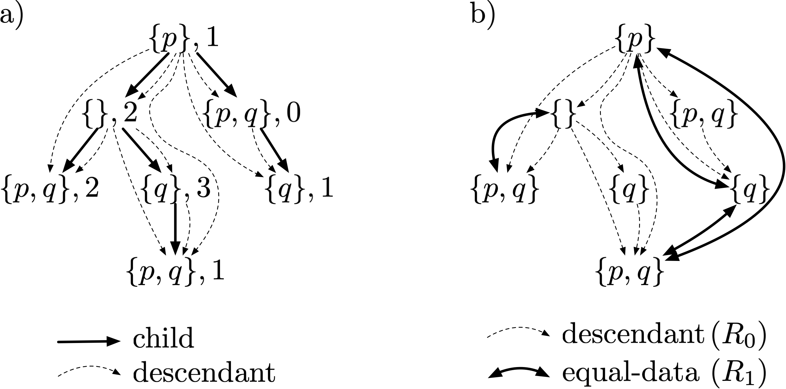
Figure 1: a) An example of a data-tree; labels are subsets of $\{p,q\}$, data-values are integers. b) The same data-tree regarded as a relational structure with ‘strict descendant’ as the relation $R_{0}$ and ‘equal-data’ as $R_{1}$. Since $R_{0}$ is the transitive closure of the accessibility relation of a tree, it is transitive irreflexive and thus the structure is a ${\rm DataGL}$ model in the sense of Definition 3.6.

As we mentioned in the Introduction, our treatment of data-aware logics is based on abstracting the actual data values and encoding the relevant information about data comparisons through specific relation symbols. Since ${\rm DataGL}$ can only compare the data values of nodes by equality or non-equality, we replace the labelling function $d$ in the definition of a data Kripke structure $\mathfrak{M}=\langle W,R,d,\ell\rangle$ for a binary relation $R_{=}^{\mathfrak{M}}\subseteq W\times W$ encoding which pairs of nodes have the same data value. Our working definition of a ${\rm DataGL}$ model is thus the following.

Definition 3.6.

Let $\sigma_{\rm DGL}=\{R_{0},R_{=},p_{1},\dots,p_{m}\}$ where $R_{0}$, $R_{=}$ are binary and $p_{1},\dots,p_{m}$ are unary. We define a ${\rm DataGL}$ model to be a $\sigma_{\rm DGL}$-structure $\mathcal{A}$ such that $|\mathcal{A}|$ is finite, $R_{0}^{\mathcal{A}}$ is transitive irreflexive, and $R_{=}^{\mathcal{A}}$ is an equivalence relation over $|\mathcal{A}|$.We denote by ${\sf ModDGL}$ the class of ${\rm DataGL}$ models.

Definition 3.7.

The syntax of ${\rm DataGL}$ is that of a modal logic with two modalities, $\Diamond_{=}$ and $\Diamond_{\neq}$, namely:

$$\varphi \ ::=R_{i}\ \mid\ \lnot\varphi\ \mid\ \varphi\land\varphi\ \mid\ \Diamond_{=}\varphi\ \mid\ \Diamond_{\neq}\varphi. i\geq 2$$ ()

For a ${\rm DataGL}$ model $\mathcal{A}$ and $a\in|\mathcal{A}|$, the semantics of ${\rm DataGL}$ are defined by

$$\mathcal{A},a\models R \text{\quad iff\quad}a\in R^{\mathcal{A}} R\in\overline{\sigma_{\rm DGL}}$$ ()

$$\mathcal{A},a\models\lnot\varphi \text{\quad iff\quad}\mathcal{A},a\not\models\varphi$$

$$\mathcal{A},a\models\varphi\land\psi \text{\quad iff\quad}\mathcal{A},a\models\varphi\text{ and }\mathcal{A},a\models\psi$$

$$\mathcal{A},a\models\Diamond_{=}\varphi \text{\quad iff\quad}\exists a^{\prime}\in|\mathcal{A}|.(a,a^{\prime})\in R_{0}^{\mathcal{A}}\cap R_{=}^{\mathcal{A}}\text{ and }{\mathcal{A}},a^{\prime}\models\varphi$$

$$\mathcal{A},a\models\Diamond_{\neq}\varphi \text{\quad iff\quad}\exists a^{\prime}\in|\mathcal{A}|.(a,a^{\prime})\in R_{0}^{\mathcal{A}}\setminus R_{=}^{\mathcal{A}}\text{ and }{\mathcal{A}},a^{\prime}\models\varphi$$

Theorem 3.8.

${\rm DataGL}$ and $\sigma_{\rm DGL}$-${\rm PPML}$ are equi-expressive over the class of ${\rm DataGL}$ models. Explicitly, there is a translation ${\rm tr}_{1}$ mapping ${\rm DataGL}$-formulas to $\sigma_{\rm DGL}$-${\rm PPML}$-formulas and a translation ${\rm tr}_{2}$ in the reverse direction such that for any ${\rm DataGL}$ model $\mathcal{A}$ and $a\in|\mathcal{A}|$,

$$\mathcal{A},a\models\varphi \text{ iff }\mathcal{A},a\models{\rm tr}_{1}(\varphi)$$

$$\mathcal{A},a\models{\rm tr}_{2}(\psi) \text{ iff }\mathcal{A},a\models\psi.$$

Owing to this result, whose proof is given in A, the only essential difference between ${\rm DataGL}$ and $\sigma_{\rm DGL}$-${\rm PPML}$ is that the latter admits more general models.

Finally, let us look at an example of how to capture more expressive logics by extending $\sigma_{\rm DGL}$.

Example 3.9.

Let $\sigma=\sigma_{\rm DGL}\cup\{T\}$ where $T$ is ternary. We wish to study the expressivity of ${\rm PPML}$ over $\sigma$ and over structures in which we require $R_{0},R_{=}$ to satisfy the ${\rm DataGL}$ constraints and require $T$ to be interpreted as $T^{\mathcal{A}}=\{(a_{1},a_{2},a_{3}):(a_{1},a_{3})\in R_{=}^{\mathcal{A}}\}$.

The ${\rm PPML}$-formula $\psi_{1}:=\Diamond(\lnot R_{=}\land\Diamond(\lnot R_{=}\land\lnot T))$ evaluated in $a$ expresses the existence of a descendant $a^{\prime}$ and a descendant $a^{\prime\prime}$ of $a^{\prime}$ such that $a,a^{\prime},a^{\prime\prime}$ have pairwise different data values. As a consequence of the fact that ‘different data’ is not transitive, it can be shown that this property is not expressible in ${\rm DataGL}$, nor in ${\rm CoreDataXPath}(\downarrow^{+})$.

On the other hand, the formula $\psi_{2}:=\Diamond(\varphi_{1}\land\Diamond(T\land\varphi_{2}))$ is true at $a$ iff $a$ has a descendant $a^{\prime}$ satisfying $\varphi_{1}$ and $a^{\prime}$ has a descendant $a^{\prime\prime}$ satisfying $\varphi_{2}$ such that $a$ and $a^{\prime\prime}$ have the same data value. It can be shown that this property is not expressible in ${\rm DataGL}$, but it is expressible in ${\rm CoreDataXPath}(\downarrow^{+})$ with the formula $\langle\varepsilon={\downarrow^{+}}[\varphi_{1}]{\downarrow^{+}}[\varphi_{2}]\rangle$.

$\psi_{1}$ is not expressible in ${\rm CoreDataXPath}(\downarrow^{+})$, thus ${\rm PPML}$ over $\sigma$ is not a fragment of ${\rm CoreDataXPath}(\downarrow^{+})$. Consider instead the signature $\tau=\{R_{0},T\}=\sigma\setminus\{R_{=}\}$. Now a property like the one given by $\psi_{1}$ cannot be expressed, while $\psi_{2}$ is still part of the language. Indeed, ${\rm PPML}$ over $\tau$ is a fragment of ${\rm CoreDataXPath}(\downarrow^{+})$.

4 ${\rm PPML}$ Bisimulation

We now present a natural notion of bounded bisimulation (and one-way simulation) for ${\rm PPML}$. These notions differ from the case of ${\rm BML}$ in that checking the ${\rm PPML}$ analogue of atomic harmony requires remembering up to $W-1$ previously visited points.

Definition 4.1.

Given two $\sigma$-structures $\mathcal{A}$ and $\mathcal{B}$, consider a chain of non-empty binary relations $\emptyset\neq Z_{k}\subseteq\dots\subseteq Z_{0}$ between sequences in $|\mathcal{A}|$ and sequences in $|\mathcal{B}|$ of the same length, such that for all $0\leq j\leq k$, the sequences related by $Z_{j}$ have length at most $n_{j}=\min\{W,k-j+1\}$. That is, $n_{k}=1$ and $n_{j-1}=n_{j}+1$ until reaching $W$, remaining constant afterwards. We say that these relations constitute a $k$-bisimulation between $\mathcal{A}$ and $\mathcal{B}$ if the following conditions hold:

1. If $sZ_{0}t$ (or equivalently, $sZ_{j}t$ for any $j$), then $R^{\mathcal{A}}(s(1),\dots,s(r))\iff R^{\mathcal{B}}(t(1),\dots,t(r))$ for all $R\in\overline{\sigma}$ of arity $r\leq|s|=|t|$;

2. Whenever $sZ_{j}t$ for some $j>0$, for each $a\in|\mathcal{A}|$ such that $\varepsilon(s)\prec a$ there is some $b\in|\mathcal{B}|$ such that $\varepsilon(t)\prec b$ and $({\rm last}_{W-1}(s).a)\ Z_{j-1}\ ({\rm last}_{W-1}(t).b)$;

3. Whenever $sZ_{j}t$ for some $j>0$, for each $b\in|\mathcal{B}|$ such that $\varepsilon(t)\prec b$ there is $a\in|\mathcal{A}|$ such that $\varepsilon(s)\prec a$ and $({\rm last}_{W-1}(s).a)\ Z_{j-1}\ ({\rm last}_{W-1}(t).b)$.

We say that $(\mathcal{A},a)$ and $(\mathcal{B},b)$ are $k$-bisimilar, notated $(\mathcal{A},a)\mathrel{\underline{~{}~{}}{\leftrightarrow}}_{k}(\mathcal{B},b)$ if there is a $k$-bisimulation $(Z_{j})_{0\leq j\leq k}$ between $\mathcal{A}$ and $\mathcal{B}$ such that $aZ_{k}b$.

A $k$-simulation from $\mathcal{A}$ to $\mathcal{B}$ is a family of non-empty relations $(Z_{j})_{0\leq j\leq k}$ as before but satisfying only item 2 above together with

1. If $j=0$, for each $R\in\overline{\sigma}$ of arity $r\leq|s|=|t|$, $R^{\mathcal{A}}(s(1),\dots,s(r))\implies R^{\mathcal{B}}(t(1),\dots,t(r))$.

We say that $(\mathcal{B},b)$ $k$-simulates $(\mathcal{A},a)$, notated $(\mathcal{A},a)\mathrel{\underline{~{}~{}}{\rightarrow}}_{k}(\mathcal{B},b)$, if there is a $k$-simulation $(Z_{j})_{j\leq k}$ from $\mathcal{A}$ to $\mathcal{B}$ such that $aZ_{k}b$.

We next prove a Hennessy-Milner-type theorem characterising logical equivalence via bisimulations. For this result to hold, $\sigma$ must be finite or the graph structures given by the interpretations of $R_{0}$ must be finitely branching (i.e. the set of immediate descendants of any point is finite). We call this condition a finiteness condition.

Theorem 4.2.

Let $\sigma$ be a permissible signature, and let $(\mathcal{A},a),(\mathcal{B},b)\in{\sf Struct}_{*}(\sigma)$. Assume that $\sigma$ is finite or $(\mathcal{A},a),(\mathcal{B},b)$ are finitely branching. Then $(\mathcal{A},a)\mathrel{\underline{~{}~{}}{\rightarrow}}_{k}(\mathcal{B},b)$ if and only if $(\mathcal{A},a)\Rrightarrow^{+}_{k}(\mathcal{B},b)$, and $(\mathcal{A},a)\mathrel{\underline{~{}~{}}{\leftrightarrow}}_{k}(\mathcal{B},b)$ if and only if $(\mathcal{A},a)\equiv_{k}(\mathcal{B},b)$.

Proof.

We show $\mathcal{A},a\mathrel{\underline{~{}~{}}{\rightarrow}}_{k}\mathcal{B},b$ iff $\mathcal{A},a\Rrightarrow^{+}_{k}\mathcal{B},b$. The proof for $\mathcal{A},a\mathrel{\underline{~{}~{}}{\leftrightarrow}}_{k}\mathcal{B},b$ iff $\mathcal{A},a\equiv_{k}\mathcal{B},b$ is analogous.

For the left-to-right implication (bisimulation invariance), we assume $\mathcal{A},a\mathrel{\underline{~{}~{}}{\rightarrow}}_{k}\mathcal{B},b$ via $(Z_{j})_{j\leq k}$ and we show that if $sZ_{j}t$, $\varphi\in{\rm PPML}^{+}_{j}$ and $\mathcal{A},s\models\varphi$, then $\mathcal{B},t\models\varphi$ by structural induction in $\varphi$. If $\varphi=R$ of arity $r$ then $r\leq|s|=|t|$ and $(s(1),\dots,s(r))\in R^{\mathcal{A}}$. Since $Z_{j}\subseteq Z_{0}$, we have $sZ_{0}t$ and by item 4 we conclude $(t(1),\dots,t(r))\in R^{\mathcal{B}}$. The case of $\varphi=\psi_{1}\land\psi_{2}$ is straightforward. Suppose $\varphi=\Diamond\psi$ and $j>0$. Then there is $a\in A$ such that $(\varepsilon(s),a)\in R_{0}^{\mathcal{A}}$ and $\mathcal{A},({\rm last}_{W-1}(s).a)\models\psi$. By item 2, there is $b\in|\mathcal{B}|$ such that $(\varepsilon(t),b)\in R_{0}^{\mathcal{B}}$ and $({\rm last}_{W-1}(s).a)Z_{j-1}({\rm last}_{W-1}(t).b)$. Observe that since $|s|=|t|\leq\min\{W,k-j+1\}$ then $|{\rm last}_{W-1}(s).a|=|{\rm last}_{W-1}(t).b|\leq\min\{W,k-j+1\}$. By the inductive hypothesis, $\mathcal{B},({\rm last}_{W-1}(t).b)\models\psi$ and then $\mathcal{B},t\models\Diamond\psi$.

For the right-to-left implication, assume $\mathcal{A},a\Rrightarrow^{+}_{k}\mathcal{B},b$. We will show that a certain family of relations $(Z_{j})_{j\leq k}$ is a $k$-simulation from $\mathcal{A}$ to $\mathcal{B}$ such that $aZ_{k}b$. This family is defined in the usual way as follows: $sZ_{j}t$ iff for all $\varphi\in{\rm PPML}^{+}_{j}$, if $\mathcal{A},s\models\varphi$ then $\mathcal{B},t\models\varphi$.

First, observe that $aZ_{k}b$ follows by the definition of $Z_{k}$. We will now verify that $(Z_{j})_{j\leq k}$ satisfies items 4 and 2. For item 4, suppose $sZ_{0}t$ and $R^{\mathcal{A}}(s(1),\dots,s(r))$ for some $R$ of arity $r\leq|s|=|t|$. Then, since relation symbols are formulas in ${\rm PPML}^{+}_{0}$, we have $R_{i}^{\mathcal{B}}(t(1),\dots,t(r))$.

For item 2, assume $sZ_{j}t$ for some $j>0$. By contradiction, suppose there is $a\in|\mathcal{A}|$ such that $\varepsilon(s)\prec a$ and for all $b\in|\mathcal{B}|$ with $\varepsilon(t)\prec b$ we have that $({\rm last}_{W-1}(s).a)Z_{j-1}({\rm last}_{W-1}(t).b)$ does not hold. Using the definition of $Z_{j-1}$, this means that for each successor $b$ of $\varepsilon(t)$ we can choose a formula $\psi_{b}\in{\rm PPML}^{+}_{j-1}$ such that $\mathcal{A},({\rm last}_{W-1}(s).a)\models\psi_{b}$ and $\mathcal{B},({\rm last}_{W-1}(t).b)\not\models\psi_{b}$. Let $\Psi$ be the set of all of these formulas, one for each $b$.

If $\mathcal{B}$ is finitely branching, then $\Psi$ is finite. Thus we can form $\varphi=\Diamond\left(\bigwedge\Psi\right)\in{\rm PPML}^{+}_{j}$, which holds for $\mathcal{A},a$ but not for $\mathcal{B},b$, contradicting the definition of $Z_{j}$. If instead $\Psi$ is not finite but $\sigma$ is finite, we replace $\Psi$ for a subset $\Psi^{\prime}\subseteq\Psi$ consisting of one formula of $\Psi$ representing each equivalence class of formulas under logical equivalence. Since $\sigma$ is finite, there are only finitely many equivalence classes in ${\rm PPML}^{+}_{j-1}$, and thus $\Psi^{\prime}$ will be finite. Thus $\varphi=\Diamond\left(\bigwedge\Psi^{\prime}\right)\in{\rm PPML}^{+}_{j}$ witnesses that $s$ and $t$ cannot be related by $Z_{j}$, giving us the desired contradiction. ∎

4.1 ${\rm PPML}$ Bisimulation Game

As in Basic Modal Logic, ${\rm PPML}$ $k$-bisimulations and $k$-simulations can be presented in terms of games. We first define the $k$-round bisimulation game $\mathcal{G}_{k}((\mathcal{A},a_{0}),(\mathcal{B},b_{0}))$, a variation of the ${\rm BML}$ bisimulation game [11], played up to $k$ rounds between $(\mathcal{A},a_{0})$ and $(\mathcal{B},b_{0})$.

The game is played between two players, called Spoiler and Duplicator. The state of the game at round $\ell\leq k$ is given by a pair of sequences $(s,t)\in|\mathcal{A}|^{\ell+1}\times|\mathcal{B}|^{\ell+1}$ corresponding to the moves of both players up to round $\ell$. We say that $(s,t)$ satisfies the winning condition for Duplicator iff for all $R\in\overline{\sigma}$ with arity $r\leq\ell+1$, ${\rm last}_{r}(s)\in R^{\mathcal{A}}\iff{\rm last}_{r}(t)\in R^{\mathcal{B}}$.

The initial position is $([a_{0}],[b_{0}])$. If $a_{0}$ and $b_{0}$ do not satisfy exactly the same unary relations, Duplicator loses the game. Otherwise, assuming position $([a_{0},\dots,a_{\ell}],[b_{0},\dots,b_{\ell}])$ is reached after $\ell\geq 0$ rounds, position $\ell+1$ is determined as follows: either Spoiler chooses $a_{\ell+1}$ such that $a_{\ell}\prec a_{\ell+1}$ and Duplicator responds with $b_{\ell+1}$ such that $b_{\ell}\prec b_{\ell+1}$, or Spoiler chooses $b_{\ell+1}$ such that $b_{\ell}\prec b_{\ell+1}$ and Duplicator responds with $a_{\ell+1}$ such that $a_{\ell}\prec a_{\ell+1}$. The resulting position for round $\ell+1$ is $([a_{0},\dots,a_{\ell+1}],[b_{0},\dots,b_{\ell+1}])$. We say that Duplicator wins the round $\ell+1$ if Duplicator is able to respond with a move which is valid according to the preceding description and which moreover makes the resulting state satisfy the winning condition. Otherwise, the game ends and Duplicator loses immediately. A winning strategy for Duplicator consists in a choice of a response that makes Duplicator win the round $\ell+1$ for every move that Spoiler may make after any number $\ell<k$ of rounds and for any possible game state $([a_{1},\dots,a_{\ell}],[b_{0},\dots,b_{\ell}])$ reachable from the initial state by the progression of the game.

We also consider the $k$-round simulation game $\mathcal{G}_{k}^{\rightarrow}((\mathcal{A},a_{0}),(\mathcal{B},b_{0}))$, in which Spoiler can only play on $\mathcal{A}$ and Duplicator on $\mathcal{B}$. In this case the winning condition for Duplicator is modified by replacing $\iff$ with $\implies$.

The following result characterises $k$-(bi)simulation in terms of winning strategies in the corresponding games. We omit the proof since it follows standard ideas from comparison games.

Theorem 4.3.

Given $(\mathcal{A},a),(\mathcal{B},b)\in{\sf Struct}_{*}(\sigma)$,

• $(\mathcal{A},a)\mathrel{\underline{~{}~{}}{\leftrightarrow}}_{k}(\mathcal{B},b)$ iff there exists a winning strategy for Duplicator in the game $\mathcal{G}_{k}((\mathcal{A},a),(\mathcal{B},b))$.

• $(\mathcal{A},a)\mathrel{\underline{~{}~{}}{\rightarrow}}_{k}(\mathcal{B},b)$ iff there exists a winning strategy for Duplicator in the game $\mathcal{G}_{k}^{\rightarrow}((\mathcal{B},b),(\mathcal{A},a))$.

Corollary 4.4.

If $\sigma$ is finite, then given $(\mathcal{A},a),(\mathcal{B},b)\in{\sf Struct}_{*}(\sigma)$,

• $(\mathcal{A},a)\equiv_{k}(\mathcal{B},b)$ iff there exists a winning strategy for Duplicator in the game $\mathcal{G}_{k}((\mathcal{A},a),(\mathcal{B},b))$.

• $(\mathcal{A},a)\equiv^{+}_{k}(\mathcal{B},b)$ iff there exist winning strategies for Duplicator both in the game $\mathcal{G}_{k}^{\rightarrow}((\mathcal{A},a),(\mathcal{B},b))$ and in $\mathcal{G}_{k}^{\rightarrow}((\mathcal{B},b),(\mathcal{A},a))$.

5 The ${\rm PPML}$ Comonad

Having captured logical indistinguishability for bounded fragments ${\rm PPML}_{k}$ and ${\rm PPML}^{+}_{k}$ through appropriate comparison games, we introduce now a $k$-indexed family of comonads which corresponds to these games and allows us to understand multiple aspects of ${\rm PPML}$ through naturally arising constructions associated to any comonad.

In the spirit of giving a self-contained account of the comonadic characterisation of ${\rm PPML}$, we recall the definitions of comonad and other related notions as they become necessary (many categorical notions will be left to C). Given a category $\mathscr{E}$, a comonad on $\mathscr{E}$ is a functor $G:\mathscr{E}\to\mathscr{E}$ equipped with natural transformations $\varepsilon:G\Rightarrow 1_{\mathscr{E}}$ and $\delta:G\Rightarrow GG$, called the counit and comultiplication of $G$, usually presented as a triple $(G,\varepsilon,\delta)$, such that the following diagrams commute for all objects $X\in\mathscr{E}$:

            

An intuition that will be useful for us is that applying $G$ to an object $X$ amounts to exposing information already contained in $X$, information that assembles into a new object $GX$ of the same kind as the original one. Readers acquainted with the notion of the unravelling of a graph might keep that in mind as an example: constructing the unravelling of a graph is a procedure which exposes some information (the paths on a graph) and organises that information into a new graph (in particular a tree). Indeed, many game comonads (including the one we will introduce shortly) constitute variants of this core idea.

From this point of view, each component $\delta_{X}$ of $\delta$ expresses the fact that the extra information in $GX$ about $X$ can be ‘duplicated’, while $\varepsilon_{X}$ consists in discarding that extra information and thus obtaining $X$ from $GX$. The diagram on the left expresses the property that for every $n$, there is one unique way to iterate this duplication of information $n$ times (this property is called co-associativity) while the diagram on the right expresses the fact that $\varepsilon$ is a right inverse of $\delta$, i.e. duplicating information and then discarding one ‘copy’ is the same as doing nothing.

We are now ready to provide the definition of our ${\rm PPML}$ comonads $(\mathbb{C}_{k})_{k\in\mathbb{N}}$.

Definition 5.1.

Let $\sigma$ be a permissible signature and let $k\geq 0$. Given a pointed $\sigma$-structure $(\mathcal{A},a)$ we define $\mathbb{C}_{k}(\mathcal{A},a)$ to be a pointed $\sigma$-structure $(\mathbb{C}_{k}(\mathcal{A},a),[a])$ with universe

$$|\mathbb{C}_{k}(\mathcal{A},a)|:=\{[a_{0},\dots,a_{\ell}]\in|\mathcal{A}|^{\leq k+1}\mid a_{0}=a\textup{ and }a_{j}\prec a_{j+1}\forall j\in\{0,\dots,\ell-1\}\}$$

and distinguished point $[a]$.

Relations are interpreted as follows. Let $\varepsilon_{\mathcal{A}}:|\mathbb{C}_{k}\mathcal{A}|\to|\mathcal{A}|$ be the function that sends a sequence to its last element. Then for each $R\in\sigma$ of arity $r$, $R^{\mathbb{C}_{k}\mathcal{A}}(s_{1},\dots,s_{r})$ iff $s_{j+1}$ is an immediate successor of $s_{j}$ in the prefix ordering of the sequences for all $j\in\{1,\dots,r-1\}$ and moreover $R^{\mathcal{A}}(\varepsilon_{\mathcal{A}}(s_{1}),\dots,\varepsilon_{\mathcal{A}}(s_{r}))$ holds. This makes $\varepsilon_{\mathcal{A}}$ into a homomorphism for all $(\mathcal{A},a)$.

We extend $\mathbb{C}_{k}$ to a functor $\mathbb{C}_{k}:{\sf Struct}_{*}(\sigma)\to{\sf Struct}_{*}(\sigma)$ by letting $\mathbb{C}_{k}$ act on morphisms: given $f:(\mathcal{A},a)\to(\mathcal{B},b)$, $\mathbb{C}_{k}f$ is given by $[a_{0},\dots,a_{\ell}]\mapsto[f(a_{0}),\dots,f(a_{\ell})]$. Functoriality is immediate.

We also define, for each $(\mathcal{A},a)\in{\sf Struct}_{*}(\sigma)$, a function $\delta:|\mathbb{C}_{k}(\mathcal{A},a)|\to|\mathbb{C}_{k}\mathbb{C}_{k}(\mathcal{A},a)|$ by $[a_{0},\dots,a_{\ell}]\mapsto[[a_{0}],[a_{0},a_{1}],\dots,[a_{0},\dots,a_{\ell}]]$, which is readily seen to determine a homomorphism $\mathbb{C}_{k}(\mathcal{A},a)\to\mathbb{C}_{k}\mathbb{C}_{k}(\mathcal{A},a)$. An immediate verification shows that $\varepsilon$ and $\delta$ thus constitute natural transformations.

We give $\mathbb{C}_{k}$ a comonad structure by declaring $\varepsilon$ to be the counit and $\delta$ to be the comultiplication. Checking that the comonad laws are satisfied is straightforward. Thus, $(\mathbb{C}_{k},\varepsilon,\delta)$ is a comonad on ${\sf Struct}_{*}(\sigma)$ for every $k\geq 0$.

Remark 5.2.

When $\sigma$ is a unimodal signature (see Remark 3.4), the structure $\mathbb{C}_{k}(\mathcal{A},a)$ is naturally isomorphic to $\mathbb{M}_{k}(\mathcal{A},a)$ where $\mathbb{M}_{k}$ is the Modal Comonad [6], in which case we call $\mathbb{M}_{k}$ the Basic Modal Comonad. The definitions of counit and comultiplication also coincide in this case, which immediately implies that they are isomorphic as comonads.

Remark 5.3.

The interpretation of relations in $\mathbb{C}_{k}(\mathcal{A},a)$ is similar to that of $\mathbb{E}_{k}(\mathcal{A},a)$ where $\mathbb{E}_{k}$ is the Ehrenfeucht-Fraïssé (EF) comonad [6], but with an additional locality constraint (tuples of sequences related by some $R\in\sigma$ must be immediate extensions of each other). Thus, $\mathbb{C}_{k}(\mathcal{A},a)$ is not an embedded substructure of $\mathbb{E}_{k}(\mathcal{A},a)$, contrary to the case of the Hybrid and Bounded comonads introduced in [3]. In this sense, the ${\rm PPML}$ comonad occupies similar but distinct middle ground between the Modal and EF comonads. Indeed, $\mathbb{C}_{k}$ is arguably closer to the Modal comonad in that it is also idempotent, see Proposition 5.8 below.

By analogy with the Modal Comonad, we sometimes say that $\mathbb{C}_{k}(\mathcal{A},a)$ is the ${\rm PPML}$-unravelling of the structure $\mathcal{A}$ starting from $a$ up to depth $k$, or its $k$-unravelling. Just like the $k$-unravelling of a Kripke structure is a Kripke tree (of height $\leq k$), the $k$-unravelling of a $\sigma$-structure (for permissible $\sigma$) is what we call a pp-tree.

Definition 5.4.

A path-predicate tree pp-tree of height $\ell$ is a pointed $\sigma$-structure $(\mathcal{T},u)$ such that (1) $(|\mathcal{T}|,R_{0}^{\mathcal{T}})$ is a tree of height $\ell$ rooted in $u$ and (2) for each $R\in\overline{\sigma}$ of arity $r$, if $u_{1},\dots,u_{r}\in|\mathcal{T}|$ are such that $R^{\mathcal{T}}(u_{1},\dots,u_{r})$, then $u_{1}\prec\dots\prec u_{r}$, i.e. $[u_{1},\dots,u_{r}]$ is the unique path of length $r$ ending in $u_{r}$.

It is immediate that given any $(\mathcal{A},a)\in{\sf Struct}_{*}(\sigma)$, $\mathbb{C}_{k}(\mathcal{A},a)$ is a pp-tree of height $\leq k$.

5.1 Fragments of First Order Logic and subcomonads

It is not hard to see that ${\rm PPML}_{k}$ translates to a fragment of First Order Logic which is has bounded quantifier rank and bounded variable number. Although we won’t state this formally, we now prove a proposition that witnesses this fact from the comonadic perspective.

Indeed, $\mathbb{C}_{k}$ turns out to be a subcomonad of the comonads corresponding to these fragments, namely the Ehrenfeucht-Fraïssé and Pebbling comonads of [6], denoted by $\mathbb{E}_{k}$ and $\mathbb{P}_{k}$. To be more precise, since these are comonads over ${\sf Struct}(\sigma)$ we must consider their liftings $\mathbb{E}_{k}^{*},\mathbb{P}_{k}^{*}$ to the category ${\sf Struct}_{*}(\sigma)$. These are defined by declaring the distinguished points of $\mathbb{E}_{k}^{*}(\mathcal{A},a)$ and $\mathbb{P}_{k}^{*}(\mathcal{A},a)$ as $[a]$ and $[(1,a)]$, respectively.

We state the Proposition here but defer its proof, together with the necessary definitions, to the B.

Proposition 5.5.

$\mathbb{C}_{k}$ is a subcomonad both of $\mathbb{E}_{k}^{*}$ and of $\mathbb{P}_{N}^{*}$, where $N=\max\{2,W\}$ is the maximum arity of all relations in $\sigma$, independent of $k$.

The subcomonad morphism $\mathbb{C}_{k}\hookrightarrow\mathbb{P}_{N}$ hints towards representing the ${\rm PPML}$ comparison games as restricted pebble games. Indeed, we see that elements of $\mathbb{C}_{k}(\mathcal{A},a)$, when interpreted as sequences of Spoiler’s moves in the ${\rm PPML}$ $k$-simulation game (see Proposition 5.6 below), get translated to certain sequences of Spoiler’s moves in the $N$-pebble game. These sequences are constrained by the fact that Spoiler (and therefore, Duplicator as well) must move the $N$ pebbles in a cyclic pattern. Thus, the resulting embedded substructure of $\mathcal{A}$ which is picked out by the positions of the $N$ pebbles always consists in the last $N$ visited positions, with a particular ordering.

5.2 $\mathbb{C}_{k}$ is the game comonad for ${\rm PPML}$

Although there is no formal definition of what makes a comonad $G$ into a game comonad, there are many properties shared by all the comonads that are informally called that way, and which may function as a makeshift definition. Two of these properties, which we take to be fundamental, are the following:

• morphisms of the type $GX\to Y$, called coKleisli morphisms in the categorical jargon, can be thought of as winning strategies for Duplicator in some existential, ‘one-way’ model comparison game played from $X$ to $Y$; and

• the category of coalgebras of $G$ is an arboreal category, and therefore pairs of objects in that category are equipped with an intrinsic notion of back-and-forth comparison game between them.

We will prove that $\mathbb{C}_{k}$ satisfies these two properties, and that the corresponding games will turn out to coincide with the ${\rm PPML}$ simulation and bisimulation games, thus making the name ‘${\rm PPML}$ comonad’ appropriate. In particular, logical equivalence for both ${\rm PPML}_{k}^{+}$ and ${\rm PPML}$ is captured by certain homomorphisms involving ${\rm PPML}$-unravellings.

We begin by discussing the first of these two properties since it can be understood merely in terms of homomorphisms involving objects built from $\mathbb{C}_{k}$. This gives an immediate sense for the meaning of this categorical construction with as little technicality as possible, and indeed the definition of $\mathbb{C}_{k}$ is reverse-engineered from the desideratum that this property holds. We will then move to the second property, which refers to the concept of coalgebras of a comonad. Instead of recalling the precise definition, we will give some intuition for them and take advantage of the fact that when a comonad is idempotent the situation simplifies greatly.

Proposition 5.6.

Given $(\mathcal{A},a),(\mathcal{B},b)\in{\sf Struct}_{*}(\sigma)$, there is a bijective correspondence between homomorphisms $\mathbb{C}_{k}(\mathcal{A},a)\to(\mathcal{B},b)$ and the set of winning strategies for Duplicator in the $k$-round simulation game $\mathcal{G}_{k}^{\rightarrow}((\mathcal{A},a),(\mathcal{B},b))$.

Proof.

The proof amounts to a close inspection of the definition of $\mathbb{C}_{k}$. Note that by definition the elements of $|\mathbb{C}_{k}(\mathcal{A},a)|$ are exactly the valid sequences of Spoiler moves. The definition of the interpretations of relations in $\mathbb{C}_{k}(\mathcal{A},a)$ is exactly such that preservation of relations by a function $|\mathbb{C}_{k}\mathcal{A}|\to|\mathcal{B}|$, i.e. the property of being a homomorphism, coincides with $f(s)$ being a valid and moreover winning answer of Duplicator to the state of the game up to that point. ∎

Corollary 5.7.

Let $(\mathcal{A},a),(\mathcal{B},b)\in{\sf Struct}_{*}(\sigma)$. Under appropriate finiteness conditions (finite $\sigma$ or finitely branching structures), $(\mathcal{A},a)\equiv_{k}^{+}(\mathcal{B},b)$ iff there exist homomorphisms $\mathbb{C}_{k}(\mathcal{A},a)\to(\mathcal{B},b)$ and $\mathbb{C}_{k}(\mathcal{B},b)\to(\mathcal{A},a)$.

From a categorical perspective, morphisms $\mathbb{C}_{k}(\mathcal{A},a)\to(\mathcal{B},b)$ can be understood as functions $(\mathcal{A},a)\to(\mathcal{B},b)$ that depend on ‘extra input’ (cf. side effects, which are ‘extra output’ of computations, captured by monads instead of comonads). We can consider homomorphisms $\mathbb{C}_{k}(\mathcal{A},a)\to(\mathcal{B},b)$ as morphisms $(\mathcal{A},a)\to(\mathcal{B},b)$ in a different category, called the coKleisli category of the comonad, $\text{\sf{Kl}}(\mathbb{C}_{k})$, which has the same objects but this new notion of (coKleisli) morphism. Thus, what this result shows is that $\text{\sf{Kl}}(\mathbb{C}_{k})$ is essentially the category of structures and $k$-simulations between them.

The category $\text{\sf{Kl}}(G)$ for a comonad $G$ is one of the two fundamental categorical constructions that can be produced from a comonad. The second one is that of the category of coalgebras, to which we now turn.

Formally, a coalgebra for a comonad $G$ on a category $\mathscr{E}$ is an object $X\in\mathscr{E}$ together with a morphism $\gamma:X\to GX$ in $\mathscr{E}$, called its structure map, such that $\varepsilon_{X}\circ\gamma=\textup{id}_{X}$ and $\delta_{X}\circ\gamma=G(\gamma)\circ\gamma$, while a morphism of coalgebras $f:(X,\gamma)\to(Y,\eta)$ is a morphism $f:X\to Y$ in $\mathscr{E}$ such that it commutes with the structure maps, i.e. $\eta\circ f=\gamma\circ G(f)$. This defines the category of coalgebras or Eilenberg-Moore category of $G$, denoted by $\text{\sf{EM}}(G)$. However, the following result allows us to simplify the discussion of $\mathbb{C}_{k}$-coalgebras enormously.

Proposition 5.8.

$\mathbb{C}_{k}$ is idempotent, i.e. the comultiplication $\delta$ is a natural isomorphism with inverse $\mathbb{C}_{k}\varepsilon$.

Proof.

For every $(\mathcal{A},a)$, we must show that $\delta_{A}\circ\mathbb{C}_{k}\varepsilon_{A}=\textup{id}_{\mathbb{C}_{k}\mathcal{A}}$ and $\mathbb{C}_{k}\varepsilon_{\mathcal{A}}\circ\delta_{\mathcal{A}}=\textup{id}_{\mathbb{C}_{k}\mathbb{C}_{k}\mathcal{A}}$. $\mathbb{C}_{k}\varepsilon_{\mathcal{A}}$ acts by sending a sequence of sequences $[s_{0},\dots,s_{\ell}]$ to the sequence $[\varepsilon_{\mathcal{A}}(s_{0}),\dots,\varepsilon_{\mathcal{A}}(s_{\ell})]$, from which the first of the two equalities is immediate. The second amounts to proving that, for any $[s_{0},\dots,s_{\ell}]\in\mathbb{C}_{k}\mathbb{C}_{k}(\mathcal{A},a)$,

$$[s_{0},\dots,s_{\ell}]=[[\varepsilon(s_{0})],[\varepsilon(s_{0}),\varepsilon(s_{1})],\dots,[\varepsilon(s_{0}),\dots,\varepsilon(s_{\ell})]].$$

We do this by induction on $\ell$. For $\ell=0$ it holds since if $[s_{0}]\in\mathbb{C}_{k}\mathbb{C}_{k}(\mathcal{A},a)$ then $s_{0}$ must be the distinguished point of $\mathbb{C}_{k}(\mathcal{A},a)$ and thus $[s_{0}]=[[a]]$. On the other hand if the equality holds for sequences of length $\ell+1$, then for any sequence $[s_{0},\dots,s_{\ell+1}]\in\mathbb{C}_{k}\mathbb{C}_{k}(\mathcal{A},a)$ of length $\ell+2$, we have

$$[s_{0},\dots,s_{\ell+1}]=[[\varepsilon(s_{0})],[\varepsilon(s_{0}),\varepsilon(s_{1})],\dots,[\varepsilon(s_{0}),\dots,\varepsilon(s_{\ell})],s_{\ell+1}].$$

Finally, $s_{\ell+1}=[\varepsilon(s_{0}),\dots,\varepsilon(s_{\ell+1})]$ since $s_{\ell+1}$ must be an immediate successor of $s_{\ell}$ in the prefix ordering. ∎

Two established consequences of a comonad $G$ on $\mathscr{E}$ being idempotent are the following (see e.g. [13, Prop 4.2.3] for the statements in dual form):

1. $\text{\sf{EM}}(G)$ is a (coreflective) subcategory of $\mathscr{E}$. This means that if an object $X\in\mathscr{E}$ admits a coalgebra structure, it is unique. Thus, we may talk about $X$ being a $G$-coalgebra as a property of the object rather than structure on it; and

2. if $X$ is a $G$-coalgebra, its structure map $X\to GX$ is an isomorphism. Therefore, all $G$-coalgebras are (isomorphic to) an object of the form $GX$ for some $X\in\mathscr{E}$.

Thanks to (1) we need only to identify which pointed $\sigma$-structures are $\mathbb{C}_{k}$-coalgebras, to identify the category $\text{\sf{EM}}(\mathbb{C}_{k})$ as the full subcategory of ${\sf Struct}_{*}(\sigma)$ spanned by those objects. From (2), we obtain immediately the desired characterisation.

Corollary 5.9.

$(\mathcal{A},a)\in{\sf Struct}_{*}(\sigma)$ is a $\mathbb{C}_{k}$-coalgebra if and only if it is a pp-tree of height $\leq k$.

Proof.

If $(\mathcal{A},a)$ is a $\mathbb{C}_{k}$-coalgebra, then by (2) above $(\mathcal{A},a)\simeq\mathbb{C}_{k}(\mathcal{A},a)$, which is a pp-tree of height $\leq k$, and the properties of being a pp-tree and having a certain height are invariant under isomorphism. Conversely, given a pp-tree of height $\ell$ it is straightforward that it is isomorphic to its ${\rm PPML}$-unravelling. ∎

Thus, $\mathbb{C}_{k}$-coalgebras are exactly the pp-trees or, equivalently, those structures that coincide (up to isomorphism) with their $k$-unravelling. Yet equivalently, these are structures that are the $k$-unravelling of some structure. The fact that relations in pp-trees can only hold along paths reflects the fact that ${\rm PPML}$ is impervious to whether relations hold between non-successor points (see Subsection 5.4).

Remark 5.10.

Following the discussion of previous game comonads, it would make sense to introduce a coalgebra number $\kappa(\mathcal{A},a)$ defined as the smallest $k$ such that $(\mathcal{A},a)$ is a $\mathbb{C}_{k}$-coalgebra, if it exists. In our case, similarly to the case of $\mathbb{M}_{k}$, this parameter makes sense only for pp-trees and coincides with the height of the pp-tree. Coalgebras of idempotent comonads are not equipped with extra structure with respect to $\sigma$-structures, thus in this sense they do not give rise to rich combinatorial parameters such as tree-depth in the case of $\mathbb{E}_{k}$ or tree-width in the case of $\mathbb{P}_{k}$.

As was mentioned before, the category $\text{\sf{EM}}(\mathbb{C}_{k})$ is arboreal for each $k$, and moreover these categories assemble into the category $\mathscr{C}:=\cup_{k}\text{\sf{EM}}(\mathbb{C}_{k})$ of all pp-trees of finite height, which in turn is a resource-indexed arboreal category (this is the content of Theorem C.11). We have chosen to present the formal definitions and proofs in the C, since they require many intermediate definitions and the proofs are more categorically involved.

Informally, an arboreal category is a category admitting a paths functor to the category of trees and tree homomorphisms, sending each object to the tree of its paths ordered by inclusion, such that each object can be obtained by gluing its associated tree of paths in a canonical way. Using this notion of paths in an object, on one hand one may define an abstract version of functional bisimulation between two objects which goes under the name of open pathwise embedding (Definition C.18), introduced in [6] as a variation on the concept of open map bisimulation [15]. On the other hand, it is possible to define a back-and-forth game between two objects $X$ and $Y$ in an arboreal category (Definition C.15), in which the positions are pairs consisting of a path in $X$ and a path in $Y$ and whose rules are essentially those of a Spoiler-Duplicator game. The general theory of arboreal categories [4, Proposition 46] then proves that Duplicator has a winning strategy in this game if and only if there exists a span between $X$ and $Y$, that is a diagram $X\leftarrow Z\to Y$, where the two morphisms are open pathwise embeddings. The fact that a span is needed, and a single morphism is not sufficient in general, reflects the elementary fact from e.g. Modal Logic that not all bisimulations are functional.

In our case, we prove that the abstract back-and-forth game coincides with the ${\rm PPML}$ Bisimulation game (Proposition C.16) and that open pathwise embeddings are precisely the strong and surjective homomorphisms between pp-trees (C.20). Thus the following characterisation of ${\rm PPML}$-bisimilarity is obtained.

Theorem 5.11.

Two structures $(\mathcal{A},a),(\mathcal{B},b)\in{\sf Struct}_{*}(\sigma)$ are $k$-bisimilar iff there exists a span of strong surjective homomorphisms $\mathbb{C}_{k}(\mathcal{A},a)\leftarrow(\mathcal{T},u)\to\mathbb{C}_{k}(\mathcal{B},b)$ with some $\mathbb{C}_{k}$-coalgebra $(\mathcal{T},u)$ as common domain.

Corollary 5.12.

Let $(\mathcal{A},a),(\mathcal{B},b)\in{\sf Struct}_{*}(\sigma)$. Under appropriate finiteness conditions, $(\mathcal{A},a)\equiv_{k}(\mathcal{B},b)$ iff there exists a span of strong surjective homomorphisms $\mathbb{C}_{k}(\mathcal{A},a)\leftarrow(\mathcal{T},u)\to\mathbb{C}_{k}(\mathcal{B},b)$ with some $\mathbb{C}_{k}$-coalgebra $(\mathcal{T},u)$ as common domain.

5.3 Alternative proof of Hennessy-Milner-type theorem for one-way simulations

Following the general relationship between coalgebras and conjunctive queries presented in [6], we can think of pp-trees as models realising ${\rm PPML}_{k}^{+}$-formulas (without disjunctions). Starting from such a formula $\varphi$, one can define a canonical, finite pp-tree $(\mathcal{T},u)$ in a standard way such that $(\mathcal{A},a)\models\varphi$ iff there exists a morphism $(\mathcal{T},u)\to(\mathcal{A},a)$. In the other direction, if $\sigma$ is finite, then from any pp-tree $(\mathcal{T},u)$ of finite height one can produce a formula $\varphi_{\mathcal{T}}$ such that $(\mathcal{T},u)$ maps homomorphically to $(\mathcal{A},a)$ if and only if $(\mathcal{A},a)\models\varphi_{\mathcal{T}}$.

Connecting this with comonads, a general and elementary fact for any comonad $G$ is that the existence of a morphism $GX\to Y$ is equivalent to the fact that for all $G$-coalgebras $Z$, if $Z$ maps into $X$ then it also maps into $Y$ (see [6, Prop. 7.1]). This line of reasoning gives an alternative proof of our Hennessy-Milner-type theorem (Theorem 4.2) for the case of finite $\sigma$. We give a sketch of the proof:

$$(\mathcal{A},a)\mathrel{\underline{~{}~{}}{\rightarrow}}_{k}(\mathcal{B},b) \text{ iff }\mathbb{C}_{k}(\mathcal{A},a)\to(\mathcal{B},b)$$

$$\text{ iff }\forall(\mathcal{T},u)\in\text{\sf{EM}}(\mathbb{C}_{k}).(\mathcal{T},u)\to(\mathcal{A},a)\implies(\mathcal{T},u)\to(\mathcal{B},b)$$

$$\text{ iff }\forall\varphi\in{\rm PPML}_{k}^{+}.(\mathcal{A},a)\models\varphi\implies(\mathcal{B},b)\models\varphi$$

$$\text{ iff }(\mathcal{A},a)\Rrightarrow_{k}^{+}(\mathcal{B},b).$$

5.4 Applications to Expressivity

In Section 6, we will make use of this categorical characterisation of logical equivalence in order to explore the relationship between ${\rm PPML}$ and Basic Modal Logic. For now, we give a different application. In the same way one can reason with games or with (bi)simulations to conclude that a certain property is not expressible within a logic such as ${\rm PPML}$, one can also do so through Corollary 5.12.

Following the literature [3, 1, 5], if $G$ is a comonad on $\mathscr{E}$ whose EM category $\text{\sf{EM}}(G)$ is arboreal, we say that

• $X,Y\in\mathscr{E}$ are back-and-forth equivalent iff there exists a span of open pathwise embeddings $GX\leftarrow Z\to GY$ in $\text{\sf{EM}}(G)$, and

• $G$ has the bisimilar companion property if $GX$ is back-and-forth equivalent to $X$ for all $X\in\mathscr{E}$.

Proposition 5.13.

Let $G$ be a comonad whose category $\text{\sf{EM}}(G)$ is arboreal. If $G$ is idempotent, then it satisfies the bisimilar companion property.

Proof.

Since isomorphisms are in particular open pathwise embeddings, our desired span of open pathwise embeddings in $\text{\sf{EM}}(G)$ is $GGX\xleftarrow{\delta_{X}}GX=GX$. ∎

In the preceding proof we have used that $\text{\sf{EM}}(G)$ can be identified with a full subcategory of $\mathscr{E}$ thanks to idempotence; this allows us to avoid using the language of adjunctions as is used in e.g. [5, Prop. 5.4].

Corollary 5.14.

$(\mathcal{A},a)\mathrel{\underline{~{}~{}}{\leftrightarrow}}\mathbb{C}_{k}(\mathcal{A},a)$ for all $(\mathcal{A},a)\in{\sf Struct}_{*}(\sigma)$. Thus, under appropriate finiteness conditions, $(\mathcal{A},a)\equiv_{k}\mathbb{C}_{k}(\mathcal{A},a)$ for all $(\mathcal{A},a)\in{\sf Struct}_{*}(\sigma)$.

Note that we arrived at this result without using the concrete description of open pathwise embeddings as strong, surjective homomorphisms. Instead, the result follows immediately from the fact that $\mathbb{C}_{k}$ is idempotent, using only the abstract definition of open pathwise embedding.

Corollary 5.14 allows us to derive many expressivity results about ${\rm PPML}$. One such result says that ${\rm PPML}$ enjoys a pp-tree-model property which generalises ${\rm BML}$’s tree-model property:

Corollary 5.15.

A ${\rm PPML}$-formula $\varphi$ is satisfiable if and only if it is satisfied by a finite pp-tree.

Proof.

Let $k$ be the modal depth of $\varphi$. Corollary 5.14 implies immediately that $\varphi$ is satisfiable if and only if it is satisfiable in some $\mathbb{C}_{k}$-coalgebra. Thus any $\varphi$ is satisfiable if and only if it is satisfied by a pp-tree of finite height. To obtain that moreover the pp-tree can be chosen to be finitely branching as well, modify the preceding argument by noting that if $\varphi$ is satisfiable, then it is satisfied in a finite model $(\mathcal{A},a)$, then take $\mathbb{C}_{k}(\mathcal{A},a)$. ∎

Indeed, for any game comonad, idempotence will imply that its corresponding logic enjoys what we could call a coalgebra-model property.

Another consequence is that any property of $\sigma$-structures that can be expressed by a ${\rm PPML}$-formula of depth $k$ must be ‘preserved’ by passing from a structure to its $k$-unravelling, since otherwise we would have two $k$-bisimilar structures which nonetheless do not satisfy the same ${\rm PPML}_{k}$-formulas. This allows us to prove that many properties are not ${\rm PPML}$-expressible. Take for instance the property “in the interpretation of $R$, there is a tuple that is not an $R_{0}$-chain” for some $R\in\overline{\sigma}$. This is obviously the case for many structures and yet it cannot be true of any pp-tree; thus it is not expressible in ${\rm PPML}$. It is in this sense that $\mathbb{C}_{k}(\mathcal{A},a)$ is what ${\rm PPML}_{k}$ ‘sees’ of a structure $(\mathcal{A},a)$.

Remark 5.16.

Analogously to the Modal Logic case, it is possible to extend ${\rm PPML}$ with graded modalities of the form $\Diamond_{n}$ with intended meaning ‘there exist at least $n$ successors such that…’. Let ${\rm PPML}(\#)$ denote this new language and ${\rm PPML}_{k}(\#)$ its fragment of modal depth $\leq k$. Since $\mathbb{C}_{k}$ is idempotent just like $\mathbb{M}_{k}$, two $\sigma$-structures $(\mathcal{A},a),(\mathcal{B},b)$ will be indistinguishable by ${\rm PPML}_{k}(\#)$ iff $\mathbb{C}_{k}(\mathcal{A},a)$ and $\mathbb{C}_{k}(\mathcal{B},b)$ are isomorphic as $\sigma$-structures. From this, it is immediate that any idempotent comonad such as $\mathbb{C}_{k}$ satisfies a property stronger than the bisimilar companion property: since $\mathbb{C}_{k}(\mathcal{A},a)\simeq\mathbb{C}_{k}\mathbb{C}_{k}(\mathcal{A},a)$ as $\sigma$-structures, under appropriate finiteness conditions, $(\mathcal{A},a)$ is not only ${\rm PPML}_{k}$-equivalent to $\mathbb{C}_{k}(\mathcal{A},a)$ but moreover it is ${\rm PPML}_{k}(\#)$-equivalent to it.

6 Relationship between ${\rm PPML}$ and Basic Modal Logic

What is ${\rm PPML}$ about, after all? ${\rm PPML}$ shares many properties with ${\rm BML}$. It contains ${\rm BML}$ for particular choices of $\sigma$ and has a coalgebra-model property, owing to its game comonad being idempotent, just like the one for ${\rm BML}$.

In what follows, we will give a way of looking at pp-trees as Kripke trees. This transformation will preserve and reflect open pathwise embeddings, as well as the truth value of formulas in a suitable sense. The first property will allow us to reduce checking $k$-bisimilarity in ${\rm PPML}$ to checking $k$-bisimilarity between Kripke trees of height $\leq k$. Meanwhile, the second property of this transformation will give polynomial reductions from the model checking and satisfiability problems for ${\rm PPML}$ to those for ${\rm BML}$.

Definition 6.1.

Given a permissible signature $\sigma$, we define a new signature $\widetilde{\sigma}=\{\widetilde{R}\ :R\in\sigma\}$ where each symbol $\widetilde{R}$ is unary except for $\widetilde{R}_{0}$, which is binary just like $R_{0}$; in fact we will identify $\widetilde{R}_{0}=R_{0}$. Given a $\sigma$-structure $(\mathcal{A},a)$, let $T(\mathcal{A},a)$, also denoted by $(\widetilde{\mathcal{A}},a)$, be the pointed $\widetilde{\sigma}$-structure with universe $|\widetilde{\mathcal{A}}|=|\mathcal{A}|$, basepoint $a$, and the following relations: $R_{0}^{\widetilde{\mathcal{A}}}=R_{0}^{\mathcal{A}}$, and for $R\in\overline{\sigma}$ of arity $n$ and $a^{\prime}\in|\mathcal{A}|$, $\widetilde{R}^{\widetilde{\mathcal{A}}}(a^{\prime})$ iff there is some $m\geq n$ and $a_{0},\dots,a_{m}$ in $|\mathcal{A}|$ such that $a_{0}=a$, $a^{\prime}=a_{m}$, $a_{i}\prec a_{i+1}$ for $i<m$ and $(a_{m-n-1},\dots,a_{m})\in R^{\mathcal{A}}$ (note that $\widetilde{R}$ coincides with $R$ for arity $n=1$). We will concentrate on this construction for the particular case of pp-trees; thus such a path will be unique if it exists.

Let $\mathbb{M}_{k}:{\sf Struct}_{*}(\widetilde{\sigma})\to{\sf Struct}_{*}(\widetilde{\sigma})$ denote the Basic Modal Comonad over signature $\widetilde{\sigma}$. Recall that this is no more and no less than the ${\rm PPML}$ comonad over $\widetilde{\sigma}$, since $\widetilde{\sigma}$ is a unimodal signature. Thus we use the notation $\mathbb{M}_{k}$ to emphasize that in our context $\mathbb{C}_{k}$ and $\mathbb{M}_{k}$ are functors defined on different categories.

Proposition 6.2.

$T$ as given above defines the action on objects of a functor $T:\text{\sf{EM}}(\mathbb{C}_{k})\to\text{\sf{EM}}(\mathbb{M}_{k})$, which acts as the identity on morphisms.

Moreover this functor is fully faithful, and its image is the full subcategory of $\text{\sf{EM}}(\mathbb{M}_{k})$ spanned by $\mathbb{M}_{k}$-coalgebras $(\mathcal{A},a)$ that satisfy the following condition:

• for any symbol $R\in\overline{\sigma}$ of arity $n$ and for any $a^{\prime}\in|\mathcal{A}|$, if $\widetilde{R}^{\mathcal{A}}(a^{\prime})$ then the height of $a^{\prime}$ is at least $n-1$.

Proof.

The claim that $T$ extends to a functor acting as the identity on morphisms reduces to the claim that given a function $f:|\mathcal{A}|\to|\mathcal{B}|$, if $f$ constitutes a homomorphism of $\sigma$-structures $(\mathcal{A},a)\to(\mathcal{B},b)$, then it also constitutes an homomorphism of $\widetilde{\sigma}$-structures $(\widetilde{\mathcal{A}},a)\to(\widetilde{\mathcal{B}},b)$. On the other hand, checking that $T$ is full reduces to checking the converse implication. It is straightforward to make these verifications. Meanwhile, faithfulness is trivial by definition.

Since $T$ is fully faithful, it defines a full subcategory of $\text{\sf{EM}}(\mathbb{M}_{k})$, and by definition of $\widetilde{R}$ ($R\in\overline{\sigma}$) it is clear that all objects in the image of $T$ satisfy condition $(\star)$. Conversely, any Kripke tree $(\mathcal{T},u)$ of finite height satisfying condition $(\star)$ is the image of a pp-tree obtained from $(\mathcal{T},u)$ by defining the interpretation of an $n$-ary $R\in\overline{\sigma}$ to contain a tuple $(a_{1},\dots,a_{n})$ if and only if it is a chain and $a_{n}\in\widetilde{R}^{\mathcal{T}}$. ∎

Intuitively, this means that for a fixed $\sigma$ we can identify pp-trees (of finite height) with the Kripke trees for which relation symbols, now interpreted as propositional letters, do not hold too close to the root, and where how close is too close is controlled by the arities of the symbols in $\sigma$.

Proposition 6.3.

$T$ preserves and reflects open pathwise embeddings.

Proof.

Since open pathwise embeddings in both the domain and codomain categories are strong surjective homomorphisms, all we must show is that a homomorphism $f:(\mathcal{A},a)\to(\mathcal{B},b)$ is strong iff $f:(\widetilde{\mathcal{A}},a)\to(\widetilde{\mathcal{B}},b)$ is strong, which is immediate. ∎

In the following corollary, we use the same symbol $\mathrel{\underline{~{}~{}}{\leftrightarrow}}_{k}$ to refer to both $k$-bisimilarity between $\sigma$-structures and $k$-bisimilarity between $\widetilde{\sigma}$-structures. Recall that since $\widetilde{\sigma}$ is unimodal, $\widetilde{\sigma}$-structures are Kripke models and the relation $\mathrel{\underline{~{}~{}}{\leftrightarrow}}_{k}$ between them is precisely $k$-bisimilarity in ${\rm BML}$ [6, Section 10.3].

Corollary 6.4.

Given two pointed $\sigma$-structures $(\mathcal{A},a)$ and $(\mathcal{B},b)$, $(\mathcal{A},a)\mathrel{\underline{~{}~{}}{\leftrightarrow}}_{k}(\mathcal{B},b)$ iff $T\mathbb{C}_{k}(\mathcal{A},a)\mathrel{\underline{~{}~{}}{\leftrightarrow}}_{k}T\mathbb{C}_{k}(\mathcal{B},b)$.

Proof.

Given two $\mathbb{C}_{k}$-coalgebras, let us write an arrow $\xrightarrow{ope}$ to indicate the existence of an open pathwise embedding between them. Let $(\mathcal{A},a)$ and $(\mathcal{B},b)$ be as above. Then

$$(\mathcal{A},a)\mathrel{\underline{~{}~{}}{\leftrightarrow}}_{k}(\mathcal{B},b) \text{ iff }\exists(\mathcal{T},u)\in\text{\sf{EM}}(\mathbb{C}_{k}).\mathbb{C}_{k}(\mathcal{A},a)\xleftarrow{ope}(\mathcal{T},u)\xrightarrow{ope}\mathbb{C}_{k}(\mathcal{B},b)$$

$$\text{ iff }\exists(\mathcal{T},u)\in\text{\sf{EM}}(\mathbb{C}_{k}).T\mathbb{C}_{k}(\mathcal{A},a)\xleftarrow{ope}T(\mathcal{T},u)\xrightarrow{ope}T\mathbb{C}_{k}(\mathcal{B},b)$$

$$\text{ iff }\exists(\mathcal{T},u)\in\text{\sf{EM}}(\mathbb{C}_{k}).\mathbb{M}_{k}T\mathbb{C}_{k}(\mathcal{A},a)\xleftarrow{ope}T(\mathcal{T},u)\xrightarrow{ope}\mathbb{M}_{k}T\mathbb{C}_{k}(\mathcal{B},b)$$

$$\text{ iff }T\mathbb{C}_{k}(\mathcal{A},a)\mathrel{\underline{~{}~{}}{\leftrightarrow}}_{k}T\mathbb{C}_{k}(\mathcal{B},b),$$

where between lines 1 and 2 we used that $T$ preserves and reflects open pathwise embeddings, while between lines 2 and 3 we used that $\mathbb{M}_{k}$ is idempotent and thus coalgebra maps $T\mathbb{C}_{k}(\mathcal{A},a)\to M_{k}T\mathbb{C}_{k}(\mathcal{A},a)$, $T\mathbb{C}_{k}(\mathcal{B},b)\to M_{k}T\mathbb{C}_{k}(\mathcal{B},b)$ are isomorphisms, hence, in particular, open pathwise embeddings. ∎

We now use the translation functor to give computational reductions from ${\rm PPML}$ problems to their ${\rm BML}$ analogues. Although the complexity results thus obtained may also be established directly, the reductions exhibit the close relationship between ${\rm PPML}$ and ${\rm BML}$.

Deciding $k$-bisimilarity

Given a finite, permissible signature $\sigma$, the problem $k\textup{{-Bisim}}(\sigma)$ has as inputs two finite, pointed $\sigma$-structures $(\mathcal{A},a)$ and $(\mathcal{B},b)$, and asks whether $(\mathcal{A},a)\mathrel{\underline{~{}~{}}{\leftrightarrow}}_{k}(\mathcal{B},b)$. Note that when $\sigma$ is unimodal, $k\textup{{-Bisim}}(\sigma)$ consists in checking whether two Kripke models are $k$-bisimilar in the usual sense of ${\rm BML}$.

Corollary 6.5.

There is a polynomial-time reduction from $k\textup{{-Bisim}}(\sigma)$ to $k\textup{{-Bisim}}(\widetilde{\sigma})$. Thus $k\textup{{-Bisim}}(\sigma)$ is in PTime.

Proof.

Given $(\mathcal{A},a)$ and $(\mathcal{B},b)$, the reduction simply computes $T\mathbb{C}_{k}(\mathcal{A},a)$ and $T\mathbb{C}_{k}(\mathcal{B},b)$, since by Corollary 6.4, $(\mathcal{B},b)$, $(\mathcal{A},a)\mathrel{\underline{~{}~{}}{\leftrightarrow}}_{k}(\mathcal{B},b)$ iff $T\mathbb{C}_{k}(\mathcal{A},a)\mathrel{\underline{~{}~{}}{\leftrightarrow}}_{k}T\mathbb{C}_{k}(\mathcal{B},b)$. Computing the action of $\mathbb{C}_{k}$ on finite structures is polynomial in the size of the structure as can be seen from inspection of Definition 5.1. On the other hand, $T$ can be computed in linear time as its action can be calculated with just one pass over the input data (for each $R\in\sigma$ and for each tuple $s\in R^{\mathbb{C}_{k}\mathcal{A}}$, write $\varepsilon(s)\in\widetilde{R}^{T\mathbb{C}_{k}\mathcal{A}}$). ∎

We now turn to the issue of truth preservation, related to giving reductions to ${\rm BML}$ for the problems of model checking and satisfiability.

Definition 6.6.

Given a $\sigma$-${\rm PPML}$-formula $\varphi$, let $\widetilde{\varphi}$ denote the $\widetilde{\sigma}$-${\rm BML}$-formula obtained by replacing each instance of each symbol $R\in\overline{\sigma}$ by $\widetilde{R}$.

Model checking

Given a permissible signature $\sigma$, the problem $\textup{{ModelCheck}}(\sigma)$ has as inputs a finite structure $(\mathcal{A},a)\in{\sf Struct}_{*}(\sigma)$ and a ${\rm PPML}$-formula $\varphi$, and asks whether $(\mathcal{A},a)\models\varphi$.

Proposition 6.7.

Given $(\mathcal{A},a)\in\text{\sf{EM}}(\mathbb{C}_{k})$ and a sliding valuation $(a_{1},\dots,a_{\ell})$ in $|\mathcal{A}|$ where $a_{1}=a$, $\mathcal{A},(a_{1},\dots,a_{\ell})\models\varphi$ if and only if $\widetilde{\mathcal{A}},a_{\ell}\models\widetilde{\varphi}$.

Proof.

We proceed by structural induction in $\varphi$. The base case is $\varphi=R$, $R\in\overline{\sigma}$ with arity $n$. If $n>\ell$ then $\mathcal{A},(a_{1},\dots,a_{\ell})\not\models\varphi$ and $\widetilde{\mathcal{A}},a_{\ell}\not\models\widetilde{\varphi}$, while if $n\leq\ell$, the equivalence holds by definition of $\widetilde{R}^{\widetilde{\mathcal{A}}}$. The cases $\varphi=\lnot\psi$ and $\varphi=\psi_{1}\land\psi_{2}$ are straightforward. Finally, for the case of $\varphi=\Diamond\psi$,

$$\mathcal{A},(a_{1},\dots,a_{\ell})\models\varphi \text{ iff }\exists a^{\prime}.a_{\ell}\prec a^{\prime}\text{ and }\mathcal{A},(a_{1},\dots,a_{\ell},a^{\prime})\models\psi$$

$$\text{ iff }\exists a^{\prime}.a_{\ell}\prec a^{\prime}\text{ and }\widetilde{\mathcal{A}},a^{\prime}\models\widetilde{\psi}$$

$$\text{ iff }\widetilde{\mathcal{A}},a_{\ell}\models{\widetilde{\varphi}}.$$

∎

Corollary 6.8.

Given $(\mathcal{A},a)\in\text{\sf{EM}}(\mathbb{C}_{k})$, $\mathcal{A},a\models\varphi$ if and only if $\widetilde{\mathcal{A}},a\models\widetilde{\varphi}$.

Corollary 6.9.

There is a polynomial-time reduction from $\textup{{ModelCheck}}(\sigma)$ to $\textup{{ModelCheck}}(\widetilde{\sigma})$.

Proof.

Just as for $k\textup{{-Bisim}}(\sigma)$, the reduction amounts to calculating $T\mathbb{C}_{k}(\mathcal{A},a)$ and checking whether $T\mathbb{C}_{k}(\mathcal{A},a)\models\widetilde{\varphi}$. ∎

Satisfiability

The problem PPML-Sat has as input a ${\rm PPML}$ formula $\varphi$, and asks whether $\varphi$ is satisfiable over $\sigma$-structures where $\sigma$ is the finite permissible signature obtained from the symbols appearing in $\varphi$ together with their specified arities. The satisfiability problem for ${\rm BML}$, BML-Sat, is defined in the same way except that all relation symbols are presumed to be unary.

Proposition 6.10.

There exists a polynomial-time reduction from PPML-Sat to BML-Sat. Moreover, since the former includes the latter, we deduce that PPML-Sat is PSpace-complete.

Proof.

Let $\varphi$ be a ${\rm PPML}$ formula, and let $\overline{\sigma}$ consist of the symbols in $\varphi$ with their prespecified arities, so that $\sigma=\{R_{0}\}\cup\overline{\sigma}$ is the permissible signature obtained from the input of PPML-Sat.

Throughout this proof, we will identify syntactically $\varphi$ with its modal translation $\widetilde{\varphi}$. That is, we will not modify the syntax of $\varphi$ by replacing symbols $R$ with symbols $\widetilde{R}$ of different arity. Instead, we will consider the symbols as unchanged and change only whether their arities are assigned according to $\sigma$ or taken to be unary.

By Corollary 6.8, if $\varphi$ is ${\rm PPML}$-satisfiable then it is ${\rm BML}$-satisfiable. However the converse does not hold since some ${\rm BML}$-satisfiable formulas such as $\psi=R$ for $R\in\overline{\sigma}$ of arity $2$, are ${\rm PPML}$-unsatisfiable. This can be seen as a consequence of the fact that $T$ is not surjective (nor essentially surjective) on objects.

Starting from $\varphi$, we define a ${\rm PPML}$-equivalent formula $\varphi^{\prime}$, computable uniformly in $\varphi$, such that $\varphi^{\prime}$ is ${\rm BML}$-satisfiable iff it is ${\rm BML}$-satisfiable by a Kripke tree of finite height satisfying ($\star$). If we manage to do this, then we will have that $\varphi$ is ${\rm PPML}$-satisfiable iff $\varphi^{\prime}$ is ${\rm BML}$-satisfiable and thus the computation of $\varphi^{\prime}$ out of $\varphi$ will be our desired reduction.

To this end, for each $R\in\overline{\sigma}$ of arity $n\geq 2$, define

$$\psi_{R}:=\lnot\bigvee_{j=0}^{n-2}(\underbrace{\Diamond\dots\Diamond}_{\text{$j$ times}}R).$$

Define $\varphi^{\prime}:=\varphi\land\varphi_{0}$ where $\varphi_{0}$ is the conjunction of all $\psi_{R}$. Note that the length of $\varphi^{\prime}$ is polynomial in the length of $\varphi$ and in the prespecified arities of the relation symbols. Note also that $\varphi$ is ${\rm PPML}$-equivalent to $\varphi^{\prime}$, since $\varphi_{0}$ is a ${\rm PPML}$-tautology.

By the tree-model property, $\varphi^{\prime}$ is ${\rm BML}$-satisfiable iff it is satisfiable in the class of finite Kripke trees. Say that $\varphi^{\prime}$ is satisfied as a modal formula by some finite Kripke tree of height $k$, i.e. a $\mathbb{M}_{k}$-coalgebra $(\mathcal{T},u)$. Then $(\mathcal{T},u)\models\varphi_{0}$ and thus it satisfies ($\star$). If on the contrary $\varphi^{\prime}$ is not ${\rm BML}$-satisfiable, then a fortiori it is not ${\rm BML}$-satisfiable by finite Kripke trees satisfying ($\star$). Thus we have established that $\varphi^{\prime}$ is ${\rm BML}$-satisfiable iff it is ${\rm BML}$-satisfiable over the class of Kripke tree of finite height which satisfy ($\star$).

By Proposition 5.15, $\varphi$ is satisfiable iff it is satisfied by some finite pp-tree, iff $\varphi^{\prime}$ is satisfied by a finite Kripke tree satisfying ($\star$) (using that $T$ preserves truth), iff $\varphi^{\prime}$ is ${\rm BML}$-satisfiable.

Since $\varphi^{\prime}$ can be computed from $\varphi$ in polynomial time, this gives a reduction from PPML-Sat to BML-Sat, which means that PPML-Sat is in PSpace. Finally, since PPML-Sat includes BML-Sat for certain choices of input, and since BML-Sat is PSpace-complete [10], PPML-Sat is PSpace-complete as well. ∎

7 Conclusions

Path Predicate Modal Logic, or ${\rm PPML}$, is a generalisation of Basic Modal Logic which arose from the insight that the ‘same data’ relationship of ${\rm DataGL}$ can be split from the definition of the modal operator(s) and added as an atom of the language. This allowed us to express ${\rm DataGL}$ not as a bimodal logic but as a unimodal logic of a new kind, and gave a more natural representation of the ${\rm DataGL}$ bisimulation game. ${\rm PPML}$ is obtained when we observe that this procedure, together with the resulting bisimulation games, generalises to any number of relation symbols of arbitrary arity.

The resulting ${\rm PPML}$ syntax has a certain redundancy built in, since it allows expressions with badly-nested instances relation symbols such as like $\varphi=R$ for $R$ binary or $\varphi=\lnot R\land\Diamond(R\lor S)$ where moreover $S$ is ternary. As long as we consider their truth-value under single-point valuations, these badly-nested instances may be safely rewritten as $\bot$. In this sense they constitute a redundancy of the syntax; however, such redundancy is necessary. In order to specify the single-point semantics in recursively, we must define a more general semantics on sliding valuations of varying length, and for this we are forced to consider as well-formed all the formulas like the ones just given.

What do we gain? We give two main motivations for ${\rm PPML}$. One is that we can think of ${\rm PPML}$ as a way of interpreting Basic Modal Logic over general $\sigma$-structures. Given a first order signature $\sigma$ that contains at least one binary relation (what we have called a ‘permissible signature’), we can select that relation to function as an accessibility relation and then use ${\rm PPML}$ to reason modally about the structure, replacing $\exists$ and $\forall$ with $\Diamond$ and $\Box$. This represents an important relaxation on what kinds of first order signatures admit a modal interpretation.

The other motivation, related to our interest in studying logics for data graphs, is that since ${\rm PPML}$ splits the concept of data-aware modalities into two separate syntactical constructs (the path-predicate modality on one side, and the atoms expressing relational properties of the data on the other), it gives us a way of capturing (and possibly designing) data-aware logics that is different from (multi-)modal logic, while at the same time retaining a modal-like syntax and semantics. In this regard it is important to keep in mind that, as we have attempted to show in this work, ${\rm PPML}$ has essentially the same expressive power and complexity that Modal Logic has. We now expand on this point.

Through the definition and study of the ${\rm PPML}$ game comonad, we identified the importance of a certain class of relational structures which we called ‘pp-trees’ and which arise as the ${\rm PPML}$-unravelling (up to a fixed, finite depth) of pointed $\sigma$-structures. Having determined that the category of finite-depth pp-trees was an indexed arboreal category, and thus that the ${\rm PPML}$ comonad had its name well deserved, the idempotence of the comonad immediately implied a pp-tree-model property, which shows among other things that ${\rm PPML}$ can only express properties of a structure that are also true of its unravelling.

Finally, our results from Section 6 relating ${\rm PPML}$ to Basic Modal Logic through polynomial-time reductions of different computational problems (deciding bounded bisimilarity, model checking and satisfiability), explain the intimate relationship between these two languages.

For a finite, permissible signature $\sigma$, the translation functor $T$ induces a function that sends $\sigma$-${\rm PPML}_{k}$-equivalence classes of relational structures to $\widetilde{\sigma}$-${\rm BML}_{k}$-equivalence classes of Kripke structures. This function is well defined since $T$ preserves $k$-bisimilarity and it is injective since the construction $\varphi\mapsto\varphi^{\prime}$ in the proof of Proposition 6.10 is truth-preserving. Therefore we can identify the semantic equivalence classes of ${\rm PPML}_{k}$ as a subset of those of ${\rm BML}_{k}$, the fragment of ${\rm BML}$ of modal depth $\leq k$. We cannot compare directly the expressivity of ${\rm BML}$ and ${\rm PPML}$, since they predicate over possibly different models; however we can take these equivalence classes as a proxy to measure ‘how many different properties’ either logic can express. It is in this sense that what ${\rm PPML}$ can express, i.e. what it can distinguish between $\sigma$-structures, is essentially what ${\rm BML}$ distinguishes between Kripke trees. Thus, what we gain is not a different expressivity but the possibility of using the same modal lens to look at more general structures.

7.1 Future work

${\rm PPML}$ over modal similarity types

Here we have presented the theory of ${\rm PPML}$ as corresponding to Basic Modal Logic, but modal languages may be constructed more generally by choosing a modal similarity type consisting of a finite number of modal operators which moreover may be polyadic, i.e. have accessibility relations of arbitrary finite arity (see [10]). In the same way, we may generalise ${\rm PPML}$ to modal similarity types. Given any relational signature $\sigma$, we may choose any finite subset of relation symbols $\tau:=\{R_{0},\dots,R_{m}\}\subseteq\sigma$, each of arity $r_{j}$, to function as accessibility relations corresponding to syntactical constructs $\Delta_{j}$. The case of $r_{j}=1$ corresponds to nullary operators $\Delta_{j}$ which serve as ‘propositional constants’, while for $r_{j}\geq 2$, the intended meaning is “$\mathcal{A},a\models\Delta_{j}(\varphi_{1},\dots,\varphi_{r_{j}-1})$ iff there exist $a_{1},\dots,a_{r_{j}-1}$ such that $R_{j}(a,a_{1},\dots,a_{r_{j}-1})$ and $\mathcal{A},(a,a_{i})\models\varphi_{i}$ for all $i\in\{1,\dots,r_{j}-1\}$”.

This is especially interesting from the point of view of our original motivation, since it allows us to view $\sigma$-structures for arbitrary signatures through a modal lens by choosing any number of arbitrary relation symbols to be interpreted as accessibility relations.

Relative comonads for ${\rm DataGL}$ and ${\rm CoreDataXPath}$

Although in this paper we concentrate on the comonadic description of ${\rm PPML}$, a DataGL comonad can be recovered as a relative comonad in the sense of [7]. To this end, recall from Definition 3.6 the notion of the ${\rm DataGL}$ first-order signature $\sigma_{\rm DGL}=\{R_{0},R_{=},p_{1},\dots,p_{m}\}$ and the notion of ${\rm DataGL}$-models as finite $\sigma_{\rm DGL}$-structures in which $R_{0}$ is interpreted as a transitive irreflexive relation and $R_{=}$ is interpreted as an equivalence relation. Let ${\sf ModDGL}$ now denote the the full subcategory of ${\sf Struct}_{*}(\sigma_{\rm DGL})$ spanned by ${\rm DataGL}$ models and let $i$ be the embedding of categories $i:{\sf ModDGL}\hookrightarrow{\sf Struct}_{*}(\sigma_{\rm DGL})$.

Note that if $(\mathcal{A},a)\in{\sf ModDGL}$, then $\mathbb{C}_{k}(\mathcal{A},a)\not\in{\sf ModDGL}$ except for trivial models, i.e. $R_{0}^{\mathbb{C}_{k}\mathcal{A}}$ will not be a tree order and $R_{=}^{\mathbb{C}_{k}\mathcal{A}}$ will not be an equivalence relation (in particular, it will not be symmetric nor transitive). This implies that $\mathbb{C}_{k}$ cannot be restricted to an comonad ${\sf ModDGL}\to{\sf ModDGL}$. However, we can still define the ${\rm DataGL}$ comonad as a relative comonad. More precisely, we define $\mathbb{C}_{k}^{\textup{\rm DGL}}:{\sf ModDGL}\to{\sf Struct}_{*}(\sigma)$ by $\mathbb{C}_{k}^{\textup{\rm DGL}}=\mathbb{C}_{k}\circ i$. This is a comonad relative to $i$ on ${\sf Struct}_{*}(\sigma_{\rm DGL})$. Specialising the results for $\mathbb{C}_{k}$ comonad to $\mathbb{C}_{k}^{\textup{\rm DGL}}$ might lead to possibly new results on ${\rm DataGL}$ using the the comonadic formalism.

Furthermore, as we begin to explore more complex comparison games, such as bisimulation games for ${\rm CoreDataXPath}$ [14], we expect that these games will be naturally captured by relative comonads which do not come from restricting a proper comonad, contrary to the case of ${\rm DataGL}$. This reinforces the centrality of relative comonads to extending the comonadic formalism to sophisticated notions of bisimulation.

Acknowledgements

This work was partially funded by UBACyT 20020190100021BA and PICT-2021-I-A-00838.

Appendix A Proof of Theorem 3.8

To show that ${\rm DataGL}$ and $\sigma_{\rm DGL}$-${\rm PPML}$ are equi-expressive over ${\sf ModDGL}$, we must translate formulas from one language to the other in both directions. Define the translation ${\rm tr}_{1}$ of ${\rm DataGL}$ into $\sigma_{\rm DGL}{\text{-}}{\rm PPML}$ as follows:

$${\rm tr}_{1}(p) =p p\in P$$ ()

$${\rm tr}_{1}(\lnot\varphi) =\lnot{\rm tr}_{1}(\varphi)$$

$${\rm tr}_{1}(\varphi\land\psi) ={\rm tr}_{1}(\varphi)\land{\rm tr}_{1}(\psi)$$

$${\rm tr}_{1}(\Diamond_{=}\varphi) =\Diamond(R_{=}\land{\rm tr}_{1}(\varphi))$$

$${\rm tr}_{1}(\Diamond_{\neq}\varphi) =\Diamond(\lnot R_{=}\land{\rm tr}_{1}(\varphi))$$

The following result can be shown by a straightforward induction in the structure of $\varphi$:

Proposition A.1.

If $\mathcal{A}$ is a ${\rm DataGL}$ model and $a\in|\mathcal{A}|$ then for any ${\rm DataGL}$-formula, we have $\mathcal{A},a\models\varphi$ iff $\mathcal{A},a\models{\rm tr}_{1}(\varphi)$.

Next, we show that $\sigma_{\rm DGL}{\text{-}}{\rm PPML}$ can be translated into ${\rm DataGL}$ when interpreted over ${\sf ModDGL}$. For simplicity, we add $\top$ and $\bot$ to the language of ${\rm PPML}$ with the obvious semantics (doing this does not increase the expressive power). We also write $\varphi\lor\psi$ as syntactic sugar for $\lnot(\lnot\varphi\land\lnot\psi)$. For a ${\rm PPML}$-formula $\varphi$, for $*\in\{\top,\bot\}$, let $\varphi[R_{=}/*]$ be the result of replacing every occurrence of $R_{=}$ which is not in the scope of a $\Diamond$ with $*$. Formally,

$$R_{=}[R_{=}/*] =*$$

$$p[R_{=}/*] =p p\in P$$ ()

$$(\lnot\varphi)[R_{=}/*] =\lnot(\varphi[R_{=}/*])$$

$$(\varphi\land\psi)[R_{=}/*] =(\varphi[R_{=}/*])\star(\psi[R_{=}/*])$$

$$(\Diamond\varphi)[R_{=}/*] =\Diamond\varphi.$$

We define a translation ${\rm tr}_{2}$ of ${\rm PPML}$ into $\sigma_{\rm DGL}{\text{-}}{\rm DataGL}$ as follows:

$${\rm tr}_{2}(R_{=}) =\bot$$

$${\rm tr}_{2}(p) =p p\in P$$ ()

$${\rm tr}_{2}(\lnot\varphi) =\lnot{\rm tr}_{2}(\varphi)$$

$${\rm tr}_{2}(\varphi\land\psi) ={\rm tr}_{2}(\varphi)\land{\rm tr}_{2}(\psi)$$

$${\rm tr}_{2}(\Diamond\varphi) =\left(\Diamond_{=}{\rm tr}_{2}(\varphi[R_{=}/\top])\right)\lor\left(\Diamond_{\neq}{\rm tr}_{2}(\varphi[R_{=}/\bot])\right)$$

Lemma A.2.

For any ${\rm DataGL}$ model $\mathcal{A}$, $a,a^{\prime}\in|\mathcal{A}|$ such that $a\prec a^{\prime}$ and any ${\rm PPML}$-formula $\varphi$ we have that $\mathcal{A},aa^{\prime}\models\varphi$ iff the following two conditions hold:

• $(a,a^{\prime})\in R_{=}^{\mathcal{A}}$ implies $\mathcal{A},a^{\prime}\models\varphi[R_{=}/\top]$, and

• $(a,a^{\prime})\notin R_{=}^{\mathcal{A}}$ implies $\mathcal{A},a^{\prime}\models\varphi[R_{=}/\bot]$.

Proof.

We proceed by induction in $||\varphi||$, the complexity $\varphi$, defined by

$$||R_{i}||=||\top||=||\bot|| =0$$

$$||\lnot\varphi||=||\Diamond\varphi|| =1+||\varphi||$$

$$||\varphi\land\psi|| =1+||\varphi||+||\psi||$$

If $\varphi=p\in P$ then the result follows from the fact that $\mathcal{A},aa^{\prime}\models\varphi$ iff $\mathcal{A},a^{\prime}\models\varphi$ and that $\varphi[R_{=}/\top]=\varphi[R_{=}/\bot]=\varphi$. The same argument applies if $\varphi$ is of the form $\Diamond\psi$, $\top$ or $\bot$. If on the other hand $\varphi=R_{=}$, then $\varphi[R_{=}/\top]=\top$ and $\varphi[R_{=}/\bot]=\bot$; $\mathcal{A},aa^{\prime}\models\varphi$ iff $(a,a^{\prime})\in R_{=}^{\mathcal{A}}$ and from this the result follows straightforwardly. The case $\varphi=\psi_{1}\land\psi_{2}$ is immediate by the inductive hypothesis. Finally, if $\varphi=\lnot\psi$ then

$$\mathcal{A},aa^{\prime}\models\varphi \text{ iff }\mathcal{A},aa^{\prime}\not\models\psi$$

$$\text{ iff }(a,a^{\prime})\in R_{=}^{\mathcal{A}}\text{ and }\mathcal{A},a^{\prime}\not\models\psi[R_{=}/\top],\text{ or }$$

$$\qquad(a,a^{\prime})\notin R_{=}^{\mathcal{A}}\text{ and }\mathcal{A},a^{\prime}\not\models\psi[R_{=}/\bot]$$ (ind. hyp.)

$$\text{ iff }(a,a^{\prime})\in R_{=}^{\mathcal{A}}\text{ and }\mathcal{A},a^{\prime}\models\varphi[R_{=}/\top],\text{ or }$$

$$\qquad(a,a^{\prime})\notin R_{=}^{\mathcal{A}}\text{ and }\mathcal{A},a^{\prime}\models\varphi[R_{=}/\bot] \dagger$$ ()

$$\text{ iff }(a,a^{\prime})\in R_{=}^{\mathcal{A}}\text{ implies }\mathcal{A},a^{\prime}\models\varphi[R_{=}/\top],\text{ and }$$

$$\qquad(a,a^{\prime})\notin R_{=}^{\mathcal{A}}\text{ implies }\mathcal{A},a^{\prime}\models\varphi[R_{=}/\bot].$$

Observe that $||\psi[R_{=}/\top]||=||\psi[R_{=}/\bot]||<||\varphi||$ and hence we can apply the inductive hypothesis; and $(\dagger)$ holds by the fact that $\varphi=\lnot\psi$ and the definition of $(\lnot\varphi)[R_{=}/*]$. ∎

Finally, the following proposition concludes the proof of Theorem 3.8.

Proposition A.3.

If $\mathcal{A}$ is a ${\rm DataGL}$ model and $a\in|\mathcal{A}|$ then for any $\sigma_{\rm DGL}{\text{-}}{\rm PPML}$-formula $\varphi$, we have $\mathcal{A},a\models\varphi$ iff $\mathcal{A},a\models{\rm tr}_{2}(\varphi)$.

Proof.

We proceed by induction in $||\varphi||$, defined in the proof of Lemma A.2. The only interesting case is when $\varphi=\Diamond\psi$, where we reason as follows:

$$\mathcal{A},a\models\Diamond\psi \text{ iff }\exists a^{\prime}.a\prec a^{\prime}\text{ such that }\mathcal{A},aa^{\prime}\models\psi$$

$$\text{ iff }\exists a^{\prime}.a\prec a^{\prime}\text{ such that }$$

$$\quad\qquad(a,a^{\prime})\in R_{=}^{\mathcal{A}}\text{ and }\mathcal{A},a^{\prime}\models\psi[R_{=}/\top],\text{ or }$$

$$\quad\qquad(a,a^{\prime})\notin R_{=}^{\mathcal{A}}\text{ and }\mathcal{A},a^{\prime}\models\psi[R_{=}/\bot]$$ (Lemma A.2)

$$\text{ iff }\exists a^{\prime}.a\prec a^{\prime}\text{ such that }$$

$$\quad\qquad(a,a^{\prime})\in R_{=}^{\mathcal{A}}\text{ and }\mathcal{A},a^{\prime}\models{\rm tr}_{2}(\psi[R_{=}/\top]),\text{ or }$$

$$\quad\qquad(a,a^{\prime})\notin R_{=}^{\mathcal{A}}\text{ and }\mathcal{A},a^{\prime}\models{\rm tr}_{2}(\psi[R_{=}/\bot])$$ (ind. hyp.)

$$\text{ iff }\exists a^{\prime}.(a,a^{\prime})\in R_{=}^{\mathcal{A}}\cap R_{=}^{\mathcal{A}}\text{ such that }\mathcal{A},a^{\prime}\models{\rm tr}_{2}(\psi[R_{=}/\top]),\text{ or }$$

$$\qquad\exists a^{\prime}.(a,a^{\prime})\in R_{=}^{\mathcal{A}}\setminus R_{=}^{\mathcal{A}}\text{ such that }\mathcal{A},a^{\prime}\models{\rm tr}_{2}(\psi[R_{=}/\bot])$$

$$\text{ iff }\mathcal{A},a\models\left(\Diamond_{=}{\rm tr}_{2}(\psi[R_{=}/\top])\right)\lor\left(\Diamond_{\neq}{\rm tr}_{2}(\psi[R_{=}/\bot])\right)$$ (def. semantics)

$$\text{ iff }\mathcal{A},a\models{\rm tr}_{2}(\Diamond\psi).$$

∎

Appendix B Proof of Proposition 5.5

We first recall the definition of a subcomonad. Given two comonads $(F,\varepsilon^{F},\delta^{F})$ and $(G,\varepsilon^{G},\delta^{G})$ over a common category, a comonad morphism $(F,\varepsilon^{F},\delta^{F})\to(G,\varepsilon^{G},\delta^{G})$ is a natural transformation $\alpha:F\Rightarrow G$ between the underlying functors such that $\varepsilon^{F}=\varepsilon^{G}\circ\alpha$ and $\delta^{G}\circ\alpha=\alpha\alpha\circ\delta^{F}$. We say that $F$ is a subcomonad of $G$ whenever there exists a comonad morphism $F\to G$ whose components are monomorphisms (in the case of ${\sf Struct}_{*}(\sigma)$, these are the injective homomorphisms).

We now recall the definitions of the EF and Pebbling comonads following [6].

For each structure $\mathcal{A}$, define a new structure $\mathbb{E}_{k}\mathcal{A}$, with universe $\mathbb{E}_{k}\mathcal{A}\,:=\,|\mathcal{A}|^{\leq k}$. For each relation symbol $R$ of arity $r$, we define $R^{\mathbb{E}_{k}\mathcal{A}}$ to be the set of $r$-tuples $(s_{1},\ldots,s_{r})$ of sequences which (1) are pairwise comparable in the prefix ordering, and such that (2) $R^{\mathcal{A}}(\varepsilon^{\mathbb{E}_{k}}_{\mathcal{A}}(s_{1}),\ldots,\varepsilon^{\mathbb{E}_{k}}_{\mathcal{A}}(s_{r}))$. The counit $\varepsilon^{\mathbb{E}_{k}}$ just referenced and the comultiplication have the exact same definitions as those of $\mathbb{C}_{k}$, given in Definition 5.1. $\mathbb{E}_{k}$ lifts to $\mathbb{E}_{k}^{*}:{\sf Struct}_{*}(\sigma)\to{\sf Struct}_{*}(\sigma)$ by letting $\mathbb{E}_{k}^{*}(\mathcal{A},a):=(\mathbb{E}_{k}\mathcal{A},[a])$.

Given a structure $\mathcal{A}$, define a new structure $\mathbb{P}_{k}\mathcal{A}$, with universe is $(\{1,\dots,k\}\times|\mathcal{A}|)^{+}$, intuitively interpreted as the set of finite non-empty sequences of moves $(p,a)$, where $p$ is a pebble index and $a\in|\mathcal{A}|$. For each relation symbol $R$ of arity $r$, we define $R^{\mathbb{P}_{k}\mathcal{A}}$ to be the set of $r$-tuples $(s_{1},\ldots,s_{r})$ of sequences such which (1) are pairwise comparable in the prefix ordering, such that (2) $R^{\mathcal{A}}(\varepsilon^{\mathbb{P}_{k}}_{\mathcal{A}}(s_{1}),\ldots,\varepsilon^{\mathbb{P}_{k}}_{\mathcal{A}}(s_{r}))$ and (3) the pebble index of the last move in each $s_{i}$ does not appear in the suffix of $s_{i}$ in $s_{j}$ for any $s_{j}$ extending $s_{i}$. The counit $\varepsilon^{\mathbb{P}_{k}}_{\mathcal{A}}$ just referenced and the comultiplication $\delta^{\mathbb{P}_{k}}$ have analogous definitions to those of $\mathbb{C}_{k}$ and $\mathbb{E}_{k}$, discarding and duplicating the information about pebble indexes respectively (in particular, $\varepsilon^{\mathbb{P}_{k}}(s)$ is the position $a\in|\mathcal{A}|$ of the last move in $s$). $\mathbb{P}_{k}$ lifts to $\mathbb{P}_{k}^{*}:{\sf Struct}_{*}(\sigma)\to{\sf Struct}_{*}(\sigma)$ by letting $\mathbb{P}_{k}^{*}(\mathcal{A},a):=(\mathbb{P}_{k}\mathcal{A},[(1,a)])$.

Proof of Proposition 5.5.

For the EF comonad, it is straightforward that the universe inclusions $|\mathbb{C}_{k}(\mathcal{A},a)|\to|\mathbb{E}_{k}(\mathcal{A},a)|$ for every $(\mathcal{A},a)$ induce injective homomorphisms and thus define a natural transformation with monic components. Compatibility with the counit and comultiplication is trivial since these are defined by the same formulas for both comonads.

For the Pebbling comonad, for each $(\mathcal{A},a)\in{\sf Struct}_{*}(\sigma)$ we define a map $\alpha_{(\mathcal{A},a)}:\mathbb{C}_{k}(\mathcal{A},a)\to\mathbb{P}_{N}(\mathcal{A},a)$ by $\alpha_{(\mathcal{A},a)}([a_{0},\dots,a_{\ell}]):=[(p_{0},a_{0}),\dots,(p_{\ell},a_{\ell})]$ where $p_{j}:=j+1\textup{(mod $N$)}$. This mapping clearly preserves the basepoint; let us see that it also preserves relation interpretations.

Suppose $R^{\mathbb{C}_{k}\mathcal{A}}(s_{1},\dots,s_{r})$ holds for some $R\in\sigma$ of arity $r$. By definition of $R^{\mathbb{C}_{k}\mathcal{A}}$, $R^{\mathcal{A}}(\varepsilon_{\mathcal{A}}(s_{1}),\dots,\varepsilon_{\mathcal{A}}(s_{r}))$ holds and $s_{j+1}$ is the immediate successor of $s_{j}$ in the prefix ordering for all $j$. This means that $R^{\mathcal{A}}(\varepsilon_{\mathcal{A}}(\alpha_{(\mathcal{A},a)}(s_{1})),\dots,\varepsilon_{\mathcal{A}}(\alpha_{(\mathcal{A},a)}(s_{r})))$ holds and that the elements $\alpha_{(\mathcal{A},a)}(s_{j})\in\mathbb{P}_{N}(\mathcal{A},a)$ are pairwise comparable in the prefix ordering. These are two of the three conditions that must be checked to establish that $R^{\mathbb{P}_{N}\mathcal{A}}(\alpha_{(\mathcal{A},a)}(s_{1}),\dots,\alpha_{(\mathcal{A},a)}(s_{r}))$ holds.

The only remaining condition to be checked is that the pebble index of the last move in each $\alpha_{(\mathcal{A},a)}(s_{j})$ does not appear in the suffix of $\alpha_{(\mathcal{A},a)}(s_{j})$ in any sequence $\alpha_{(\mathcal{A},a)}(s_{j}^{\prime})$ extending $\alpha_{(\mathcal{A},a)}(s_{j})$. Since each $\alpha_{(\mathcal{A},a)}(s_{j+1})$ is an immediate successor of $\alpha_{(\mathcal{A},a)}(s_{j})$, it is enough to check this for $j^{\prime}=r$. If $|s_{1}|=\ell+1$, we may write

$$s_{r} =[a_{0},\dots,a_{\ell},\dots,a_{\ell+r-1}]$$

$$\alpha_{(\mathcal{A},a)}(s_{r}) =[(p_{0},a_{0}),\dots,(p_{\ell},a_{\ell}),\dots,(p_{\ell+r-1},a_{\ell+r-1})].$$

We must show that the last position where $p_{j}$ appears in $\alpha_{(\mathcal{A},a)}(s_{r})$ is the $j$-th position, for all $\ell\leq j\leq\ell+r-1$. By definition of $\alpha_{(\mathcal{A},a)}$, the next position where $p_{j}$ appears after position $j$ would be position $j+N$, but this will always be out of range because $r\leq N$.

This proves that indeed the mappings $\alpha_{(\mathcal{A},a)}$ are well defined morphisms in ${\sf Struct}_{*}(\sigma)$. The remaining verifications, namely those of naturality and preservation of counit and comultiplication, are all straightforward. ∎

Appendix C Proof of Theorem 5.11

In this section we aim to prove Theorem 5.11. We consider the proof technique to be of interest in itself since it makes use of the abstract theory of arboreal categories and elucidates why $\mathbb{C}_{k}$ is the game comonad corresponding to ${\rm PPML}$.

The plan is as follows: first we prove a more abstract version of Theorem 5.11 (C.17), which refers to open pathwise embeddings instead of strong surjective homomorphisms. We accomplish this by first proving that the ${\rm PPML}$ comonads $\{\mathbb{C}_{k}\}_{k}$ induce a resource-indexed arboreal cover of ${\sf Struct}_{*}(\sigma)$ (Theorem C.11), and then proving that the abstract back-and-forth games in the EM categories of the comonads $\mathbb{C}_{k}$ correspond to the ${\rm PPML}$ Bisimulation game for different choices of $k$ (Proposition C.16). This allows us to use [4, Proposition 46] in order to relate $k$-bisimilarity to the existence of spans of open pathwise embeddings (Theorem C.17). Finally, we obtain Theorem 5.11 from the fact that open pathwise embeddings in our case are the strong surjective homomorphisms (Proposition C.20).

Above we have already assumed knowledge of the basic categorical concepts of categories, functors, and natural transformations. Here we will also assume familiarity with limits and colimits (including pullbacks, products and coproducts). We will also mention adjunctions since the theory of arboreal categories is formulated in that language.

The following definitions are reproduced from [4] to facilitate reading. We assume $\mathscr{C}$ is a locally small and well-powered category.

Definition C.1.

Given a category $\mathscr{C}$ and a pair of arrows $e$ and $m$ in $\mathscr{C}$, we say that $e$ has the left lifting property with respect to $m$, or that $m$ has the right lifting property with respect to $e$, iff for every commutative square

there exists a possibly non-unique diagonal filler $d$ such that

commutes.

A pair of classes of morphisms $(\mathscr{M},\mathscr{Q})$ is a weak factorisation system on $\mathscr{C}$ iff every morphism in $\mathscr{C}$ can be factorised as $f=m\circ e$ with $e\in\mathscr{Q}$ and $m\in\mathscr{M}$ and moreover $\mathscr{Q}$ is precisely the the class of morphisms having the left lifting property against every morphism in $\mathscr{M}$ while $\mathscr{M}$ is precisely the the class of morphisms having the right lifting property against every morphism in $\mathscr{Q}$.

A factorisation system $(\mathscr{M},\mathscr{Q})$ is said to be proper iff all $\mathscr{Q}$-morphisms are epimorphisms and all $\mathscr{M}$-morphisms are monomorphisms. It is said to be a stable proper factorisation system iff it is proper and moreover for any $e\in\mathscr{Q}$ and $m\in\mathscr{M}$ with common codomain, the pullback of $e$ along $m$ exists and belongs to $\mathscr{Q}$.

Definition C.2.

Let $\mathscr{C}$ be a category equipped with a stable proper factorisation system $(\mathscr{M},\mathscr{Q})$ and let $X\in\mathscr{C}$. An $\mathscr{M}$-subobject of $X$ is an $\mathscr{M}$-morphism with codomain $X$, considered up to the following equivalence relation: given $\mathscr{M}$-morphisms $m:Y\to X$ and $n:Z\to X$, $m\sim n$ iff there exists an isomorphism $i$ such that $m=n\circ i$. The set of $\mathscr{M}$-subobjects of $X$ has a natural partial ordering given by $[m]\leq[n]$ iff there exists a morphism $i$ such that $m=n\circ i$. We say that $[m]\prec[n]$ iff $[n]$ is an immediate successor of $[m]$.

We say $X$ is a path iff its poset of $\mathscr{M}$-subobjects is a finite chain. We denote by $\mathbb{S}X$ the poset of $\mathscr{M}$-subobjects of $X$ and by $\mathbb{P}X$ the subposet of path embeddings, that is the $\mathscr{M}$-subobjects of $X$ whose domains are paths.

Remark C.3.

All the categories that will appear in our discussion are full subcategories of ${\sf Struct}_{*}(\sigma)$, whose factorisation system $(\mathscr{M},\mathscr{Q})$ will be taken to be (embeddings, surjective homomorphisms). Thus, paths in our case will always be pointed $\sigma$-structures $(\mathcal{P},p)$ such that $(|\mathcal{P}|,R_{0}^{\mathcal{P}})$ is a finite chain with minimal element $p$.

Remark C.4.

When talking about paths in a structure $(\mathcal{A},a)$ we may take them to be the path embeddings $m:(\mathcal{P},p)\to(\mathcal{A},a)$ or, equivalently, consider them to be simply the embedded substructures of $(\mathcal{A},a)$ which are moreover paths. In any case, note that by definition paths in $(\mathcal{A},a)$ are finite and start at $a$, and that there is a bijection between $\mathbb{P}(\mathcal{A},a)$ and points of $\mathbb{C}_{k}(\mathcal{A},a)$.

Definition C.5.

A category $\mathscr{C}$ is said to be a path category iff the following hold:

• $\mathscr{C}$ has a stable proper factorisation system $(\mathscr{M},\mathscr{Q})$;

• $\mathscr{C}$ has all coproducts of small families of paths;

• for any paths $P,Q,R$, if a composite $P\to Q\to R$ is a $\mathscr{Q}$-morphism, then so is $P\to Q$ (the so-called “two out of three property”).

Definition C.6.

An object $X$ in a path category $\mathscr{C}$ is connected iff for all small families of paths $(P_{i})_{i\in I}$ in $\mathscr{C}$, any morphism $X\to\amalg_{i\in I}P_{i}$ factors through some coproduct injection $P_{j}\to\amalg_{i\in I}P_{i}$.

Definition C.7.

Given an object $X$ in a path category $\mathscr{C}$, consider the cocone with nadir $X$ consisting of all path embeddings with codomain $X$:

where the morphisms between paths are those morphisms in $\mathscr{C}$ which make the evident triangles commute. More formally, let $(\mathscr{C}/X)_{\mathscr{M}}$ be the full subcategory of $\mathscr{C}/X$, the category over $X$, on the $\mathscr{M}$-morphisms. Let $\Pi_{X}:(\mathscr{C}/X)_{\mathscr{M}}\to\mathscr{C}$ be the projection functor. Then the cocone in question is the cocone $\lambda:\Pi_{X}\Rightarrow X$ whose leg $\lambda_{(P,f)}$ is $f$. We say that $X$ is path-generated iff this cocone is a colimit cocone in $\mathscr{C}$.

Definition C.8.

An arboreal category is a path category $\mathscr{C}$ such that (1) every object of $\mathscr{C}$ is path-generated, and (2) every path in $\mathscr{C}$ is connected.

Definition C.9.

A collection $\{\mathscr{C}_{k}\}_{k\in\mathbb{N}}$ of categories is a resource-indexed arboreal category iff the following hold:

1. There is an arboreal category $\mathscr{C}$ with full subcategory of paths $\mathscr{C}_{p}$ such that for all $k\geq 0$, there is a full subcategory $\mathscr{C}_{p}^{k}$ of $\mathscr{C}_{p}$ closed under embeddings with $\mathscr{C}_{p}^{0}\hookrightarrow\mathscr{C}_{p}^{1}\hookrightarrow\mathscr{C}_{p}^{2}\hookrightarrow\dots$

2. For every $k$, the full subcategory of $\mathscr{C}$ spanned by the “$k$-path-generated objects” is precisely $\mathscr{C}_{k}$. More specifically, the objects of $\mathscr{C}_{k}$ are precisely those objects whose cocone of path embeddings with domain in $\mathscr{C}_{p}^{k}$ is a colimit cocone in $\mathscr{C}$.

Definition C.10.

Given a resource-indexed arboreal category $\{\mathscr{C}_{k}\}_{k\in\mathbb{N}}$, a resource-indexed arboreal cover of a category $\mathscr{E}$ by $\{\mathscr{C}_{k}\}_{k\in\mathbb{N}}$ is an indexed family of comonadic adjunctions

(1)

Since any adjunction induces a comonad, a resource-indexed arboreal cover induces an indexed family of comonads $\{(G_{k},\delta^{k},\varepsilon^{k})\}_{k\in\mathbb{N}}$ where $G_{k}=L_{k}R_{k}$, $\delta^{k}=L_{k}\eta_{k}R_{k}$ and $\eta^{k},\varepsilon^{k}$ are the unit and counit of each adjunction, respectively.

By definition, an adjunction is comonadic iff the domain of the left adjoint is isomorphic to the EM category of the induced comonad. Thus, that the adjunctions are comonadic means that $\mathscr{C}_{k}\simeq\text{\sf{EM}}(G_{k})$ for each $k$.

$\{\mathbb{C}_{k}\}_{k}$ induces a resource-indexed arboreal cover

Our first aim is to prove the following theorem.

Theorem C.11.

$\{\text{\sf{EM}}(\mathbb{C}_{k})\}$ constitutes a resource-indexed arboreal category. Therefore, the family of comonadic adjunctions

where $i_{k}$ is the inclusion of categories and $C_{k}$ is the co-restriction of $\mathbb{C}_{k}$ to its image, constitutes a resource-indexed arboreal cover of ${\sf Struct}_{*}(\sigma)$.

By definition, the adjunctions involved are comonadic and the induced comonads on ${\sf Struct}_{*}(\sigma)$ are precisely $\{\mathbb{C}_{k}\}_{k}$. Thus all we must really do is prove that $\{\text{\sf{EM}}(\mathbb{C}_{k})\}$ constitutes a resource-indexed arboreal category. This amounts to straightforward verifications, however we consider it worthwhile include the verifications in detail in order to illustrate the procedure.

Once we prove that $\{\text{\sf{EM}}(\mathbb{C}_{k})\}_{k}$ is a resource-indexed arboreal category, we will also have established that in particular each category $\text{\sf{EM}}(\mathbb{C}_{k})$ is arboreal [4, Prop. 42].

Let $\mathsf{ppTree}$ be the category of $\mathbb{C}_{k}$-coalgebras for all $k$, that is, the full subcategory of ${\sf Struct}_{*}(\sigma)$ spanned by pp-trees of finite height.

Lemma C.12.

$\mathsf{ppTree}$ is arboreal.

We give the proof incrementally, building on two preliminary propositions.

Proposition C.13.

$\mathsf{ppTree}$ has a stable proper factorisation system $(\mathscr{Q},\mathscr{M})$ where $\mathscr{Q}$ are the (basepoint-preserving) surjective homomorphisms and $\mathscr{M}$ are the (basepoint-preserving) embeddings of relational structures.

Proof.

We start from the fact that $(\mathscr{Q},\mathscr{M})$ as above is a stable, proper factorisation system for ${\sf Struct}(\sigma)$ [4, Example 2.4]. First we check that the system lifts to ${\sf Struct}_{*}(\sigma)$ and then that it restricts well to the full subcategory $\mathsf{ppTree}$.

This factorisation system lifts to ${\sf Struct}_{*}(\sigma)$ in the following way: let $U:{\sf Struct}_{*}(\sigma)\to{\sf Struct}(\sigma)$ be the evident forgetful functor. Given $f:(\mathcal{A},a)\to(\mathcal{B},b)$, the factorisation $\mathcal{A}\xrightarrow{e}\widetilde{\mathcal{A}}\xrightarrow{m}\mathcal{B}$ of $Uf$ lifts to a factorisation of $f$ by simply declaring the basepoint of $\widetilde{\mathcal{A}}$ to be $e(a)$. It is straightforward that diagonal fillers in ${\sf Struct}(\sigma)$ must preserve basepoints and thus also lift to ${\sf Struct}_{*}(\sigma)$. This establishes the lifting of $(\mathscr{Q},\mathscr{M})$ as a weak factorisation system. The lifted factorisation system is proper because basepoint-preserving surjective homomorphisms are epimorphisms in ${\sf Struct}_{*}(\sigma)$ and basepoint-preserving relational embeddings are monomorphisms in ${\sf Struct}_{*}(\sigma)$. To see that the factorisation system is stable, recall that ${\sf Struct}_{*}(\sigma)$ is category under $*$, $*/{\sf Struct}(\sigma)$, where $*$ is the structure with one point in which the interpretations of all relations are empty, and that the projection functor $\Pi:*/{\sf Struct}(\sigma)\to{\sf Struct}(\sigma)$ strictly creates all limits (since ${\sf Struct}(\sigma)$ is complete), in particular pullbacks (see e.g. [16, Proposition 3.3.8]).

The factorisation system on ${\sf Struct}_{*}(\sigma)$ restricts well to $\mathsf{ppTree}$ because it is a full subcategory and given any morphism between pp-trees, the intermediate object of its ($\mathscr{M},\mathscr{Q}$)-factorisation is also a pp-tree. The resulting weak factorisation system on $\mathsf{ppTree}$ is obviously proper (inclusions reflect monomorphisms and epimorphisms). As for stability, we use that the inclusion $i:\mathsf{ppTree}\hookrightarrow{\sf Struct}_{*}(\sigma)$, being fully faithful, reflect limits. This means that given a cone $\lambda:X\Rightarrow J$ over a diagram $J:I\to\mathsf{ppTree}$, if $\lambda$ is a limit cone over $J$ when seen in ${\sf Struct}_{*}(\sigma)$, then it is also a limit cone when seen in $\mathsf{ppTree}$. Thus, if we check that the pullback of pp-trees is also a pp-tree, that means that the pullback of pp-trees in ${\sf Struct}_{*}(\sigma)$ is the pullback in $\mathsf{ppTree}$, and then since the factorisation system is stable in ${\sf Struct}_{*}(\sigma)$ (pullbacks of $\mathscr{Q}$-morphisms along $\mathscr{M}$-morphisms exist and are $\mathscr{Q}$-morphisms), its restriction to $\mathsf{ppTree}$ will be stable as well.

Recall that given a diagram in ${\sf Struct}_{*}(\sigma)$, its limit has as universe the set-theoretical limit of the underlying universes (since the forgetful functor to $\mathsf{Set}$ is a right adjoint). Thus it is easy to check that the categorical product of relational structures coincides with the standard notion of product of structures, while it is also easy to check that the categorical equaliser of two relational homomorphisms $f,g:(\mathcal{A},a)\to(\mathcal{B},b)$ can be constructed as the embedded substructure $(\mathcal{Z},z)\to(\mathcal{A},a)$ consisting of points $a^{\prime}\in|\mathcal{A}|$ such that $f(a^{\prime})=g(a^{\prime})$. It is straightforward to verify that product of two pp-trees is a pp-tree and that the equaliser of two homomorphisms between pp-trees is also a pp-tree. Hence, since a pullback is nothing more than the equalizer of a product of homomorphisms, the pullback of two pp-trees is also a pp-tree. ∎

Proposition C.14.

$\mathsf{ppTree}$ is a path category.

Proof.

We have just seen that $(\mathscr{M},\mathscr{Q})$ as above is a stable proper factorisation system for $\mathsf{ppTree}$. To see that $\mathsf{ppTree}$ has all coproducts of small families of paths, we show that a fortiori all small coproducts exist in $\mathsf{ppTree}$. Recall that finite coproducts exist in ${\sf Struct}_{*}(\sigma)$. The universe of the binary coproduct $(\mathcal{A},a)\amalg(\mathcal{B},b)$ is formed by taking the disjoint union of the universes $|\mathcal{A}|$ and $|\mathcal{B}|$, and then identifying the basepoints. A relation $R$ holds on a tuple of points in this universe iff all the points can be traced back to either $\mathcal{A}$ or $\mathcal{B}$ exclusively, and moreover the tuple belonged to the interpretation of $R$ in that structure.

Now, from the description above it should be clear that if $(\mathcal{A},a)$ and $(\mathcal{B},b)$ are pp-trees, then $(\mathcal{A},a)\amalg(\mathcal{B},b)$ is too: it is a tree with height equal to the maximum of the heights of the starting trees, and if a tuple belongs to a relation, then that must have been the case in one of the starting structures and thus the tuple constitutes a path in the structure. Finally, because inclusions of categories reflect colimits, $(\mathcal{A},a)\amalg(\mathcal{B},b)$ must also be the categorical coproduct in $\mathsf{ppTree}$.

This establishes the existence of all finite coproducts. To extend this to all small coproducts, note that the above construction can be generalized in a straightforward way to a nonempty collection of $\mathbb{C}_{k}$-coalgebras. As for the empty collection, its coproduct is the initial object, which is the one-element universe in which no relations hold.

Finally, to see that $\mathsf{ppTree}$ satisfies the two out of three property for paths, start by noticing that in a path there is exactly zero or one element for each height. Homomorphisms between paths are injective, and thus they preserve and reflect height. Given paths $P,Q,R$, homomorphisms $P\xrightarrow{f}Q\xrightarrow{g}R$ such that $g\circ f$ is a $\mathscr{Q}$-morphism (i.e. a surjective homomorphism) and given $q\in Q$, let $p\in P$ be the preimage of $g(q)$. Then $f(p)=q$ since $q$ is the only element of $Q$ of the appropriate height. Thus $f$ is also a $\mathscr{Q}$-morphism. ∎

Proof of Lemma C.12.

We have already seen that $\mathsf{ppTree}$ is a path category. That every path in $\mathsf{ppTree}$ is connected is straightforward from the construction of small coproducts above, since a coproduct of paths $\amalg_{i\in I}P_{i}$ is a tree whose only branching node (point with more than one successor) is the root node. Thus the image of a homomorphism $Q\to\amalg_{i\in I}P_{i}$ lies entirely in one of the $P_{i}$.

Let us now see that every object of $\mathsf{ppTree}$ is path-generated. Given $(\mathcal{A},a)\in\mathsf{ppTree}$, consider the diagram $\Pi_{(\mathcal{A},a)}:(\mathsf{ppTree}/(\mathcal{A},a))_{\mathscr{M}}\to\mathsf{ppTree}$ of all path embeddings into $(\mathcal{A},a)$, and consider the canonical cocone under that diagram $\eta:\Pi_{(\mathcal{A},a)}\Rightarrow X$ whose leg $\eta_{(P,f)}$ is $f$. In order to prove that this is a colimit cocone in $\mathsf{ppTree}$, by taking representatives, we can assume that all paths $P$ in the diagram are embedded relational substructures inside $\mathcal{A}$, and thus the legs of this cocone are the corresponding inclusions $i_{P}$. Now consider a generic cocone $\lambda:\Pi_{(\mathcal{A},a)}\Rightarrow(\mathcal{B},b)$ in $\mathsf{ppTree}$ over the same diagram, this time with nadir $(\mathcal{B},b)$. We must show existence of a unique homomorphism $\varphi:(\mathcal{A},a)\to(\mathcal{B},b)$ such that it commutes with the legs of the cocones.

Given $a^{\prime}\in|\mathcal{A}|$, let $\mathcal{A}_{a^{\prime}}$ denote the unique path from $a$ to $a^{\prime}$. It is clear that if $\varphi$ exists, then it must send $a^{\prime}\mapsto\lambda_{\mathcal{A}_{a^{\prime}}}(a^{\prime})$. This choice of $\varphi$ makes the corresponding triangles commute (i.e. $\varphi\circ i_{P}=\lambda_{P}$); indeed, for any path $P$ containing $a^{\prime}$, it must be the case that $\mathcal{A}_{a^{\prime}}\subseteq P$ and thus $\lambda_{P}$ and $\lambda_{\mathcal{A}_{a^{\prime}}}$ agree on $a^{\prime}$ since $\lambda$ is a cocone.

Now let us see that $\varphi$ is a homomorphism. It is straightforward that $\varphi(a)=b$. To see that $\varphi$ preserves relations, let $R\in\sigma$ be of arity $n$ and assume $R^{\mathcal{A}}(a_{1},\dots,a_{n})$ holds. Then $a_{1},\dots,a_{n}$ must be all contained in $\mathcal{A}_{a_{n}}$, and thus since $\lambda_{\mathcal{A}_{a_{n}}}$ is a homomorphism, it must be that $R^{\mathcal{B}}(\lambda_{\mathcal{A}_{a_{n}}}(a_{1}),\dots,\lambda_{\mathcal{A}_{a_{n}}}(a_{n}))$, i.e. $R^{\mathcal{B}}(\varphi(a_{1}),\dots,\varphi(a_{n}))$. ∎

Finally, a small observation completes the proof of Theorem C.11.

Proof of Theorem C.11.

We have just proven that $\mathsf{ppTree}$ is arboreal. By Remark C.3, for every $k$, the full subcategory of paths in $\mathsf{ppTree}$, which we denote by $\mathsf{ppTree}_{p}$, consists of those pp-trees which are moreover total orders. Let $\mathsf{ppTree}_{p}^{k}$ be the full subcategory of $\mathsf{ppTree}_{p}$ of paths of length at most $k$. This is clearly closed under embeddings. It is also straightforward that $\mathsf{ppTree}_{p}^{k}$ embeds into $\mathsf{ppTree}_{p}^{k+1}$ for all $k$.

To show that $\{\text{\sf{EM}}(\mathcal{C}_{k})\}_{k\in\mathbb{N}}$ is a resource-indexed arboreal category, we must see that the objects of $\text{\sf{EM}}(\mathbb{C}_{k})$ are precisely those objects whose cocone of path embeddings with domain in $\mathsf{ppTree}_{p}^{k}$ is a colimit cocone in $\mathsf{ppTree}$. To this end, it is enough to show that in the proof of Lemma C.12, if the object of $\mathsf{ppTree}$, in particular a tree, has height at most $k$ and thus belongs to $\text{\sf{EM}}(\mathbb{C}_{k})$, then all the paths in the diagram are actually objects of $\mathsf{ppTree}_{p}^{k}$, that is, they all have length at most $k$. Indeed, a path of length $>k$ cannot be embedded into a tree of height $\leq k$. Thus, for $(\mathcal{A},a)\in\text{\sf{EM}}(\mathbb{C}_{k})$, the cocone of path embeddings with codomain $(\mathcal{A},a)$ which was shown above to be a colimit cocone in $\mathsf{ppTree}$ is also the cocone of path embeddings with nadir $(\mathcal{A},a)$ and domains in $\mathsf{ppTree}_{p}^{k}$. ∎

The abstract back-and-forth game in $\mathsf{ppTree}_{k}$ is the ${\rm PPML}$ Bisimulation game

We now reproduce from [4] the definition of the abstract back-and-forth game between objects of an arboreal category.

Definition C.15.

Let $\mathscr{C}$ be an arboreal category and let $X,Y\in\mathscr{C}$. The back-and-forth game $\mathscr{G}(X,Y)$ between $X$ and $Y$ is defined as follows.

The game is played between two players, called Spoiler and Duplicator. The state of the game at round $\ell$ is given by a pair of (equivalence classes of) path embeddings $([m],[n])\in\mathbb{P}X\times\mathbb{P}Y$. We say that $([m],[n])$ satisfies the winning condition if the domains ${\rm dom}(m)$ and ${\rm dom}(n)$ are isomorphic.

The initial position is $(\bot_{X},\bot_{Y})$ where $\bot_{X}\colon P\to X$ and $\bot_{Y}\colon Q\to Y$ are the roots of $\mathbb{P}{X}$ and $\mathbb{P}{Y}$, respectively. If $P$ and $Q$ are not isomorphic, then Duplicator loses the game. Otherwise, assuming position $([m],[n])\in\mathbb{P}{X}\times\mathbb{P}{Y}$ is reached after $\ell\geq 0$ rounds, position $\ell+1$ is determined as follows: either Spoiler chooses some $[m^{\prime}]\succ[m]$ and Duplicator must respond with some $[n^{\prime}]\succ[n]$, or Spoiler chooses some $[n^{\prime\prime}]\succ[n]$ and Duplicator must respond with $[m^{\prime\prime}]\succ[m]$. We say that Duplicator wins the round $\ell+1$ if Duplicator is able to respond with a move which is valid according to the preceding description and which moreover makes the resulting state satisfy the winning condition. Otherwise, the game ends and Duplicator loses immediately. A winning strategy for Duplicator consists in a choice of a response that makes Duplicator win the round $\ell+1$ for every move that Spoiler may make after any number of rounds $\ell>0$.

Recall that each category in a resource-indexed arboreal category is in particular arboreal. Thus we can speak of the back-and-forth-game in each category $\text{\sf{EM}}(\mathbb{C}_{k})$.

Proposition C.16.

The $k$-round bisimulation game for ${\rm PPML}$ played between $(\mathcal{A},a)$ and $(\mathcal{B},b)$, $\mathcal{G}_{k}((\mathcal{A},a),(\mathcal{B},b))$, is equivalent to the back-and-forth game $\mathscr{G}(\mathbb{C}_{k}(\mathcal{A},a),\mathbb{C}_{k}(\mathcal{B},b))$ in the arboreal category $\text{\sf{EM}}(\mathbb{C}_{k})$ played between $\mathbb{C}_{k}(\mathcal{A},a)$ and $\mathbb{C}_{k}(\mathcal{B},b)$. More precisely, there exists a winning strategy for Duplicator in one of the two games iff there exists one in the other.

Proof.

A position in the abstract back-and-forth game $\mathscr{G}(\mathbb{C}_{k}(\mathcal{A},a),\mathbb{C}_{k}(\mathcal{B},b))$ is a pair $([m],[n])\in\mathbb{P}\mathbb{C}_{k}(\mathcal{A},a)\times\mathbb{P}\mathbb{C}_{k}(\mathcal{B},b)$, which by Remark C.4 can be seen as a pair of elements from $\mathbb{C}_{k}\mathbb{C}_{k}(\mathcal{A},a)\times\mathbb{C}_{k}\mathbb{C}_{k}(\mathcal{B},b)$. But $\mathbb{C}_{k}$ is idempotent, thus $\delta$ gives an identification between positions $(m,n)$ in $\mathscr{G}(\mathbb{C}_{k}(\mathcal{A},a),\mathbb{C}_{k}(\mathcal{B},b))$ and positions $(s,t)\in\mathbb{C}_{k}(\mathcal{A},a)\times\mathbb{C}_{k}(\mathcal{B},b)$ in the game in $\mathcal{G}_{k}((\mathcal{A},a),(\mathcal{B},b))$. This correspondence also maps the starting position $(\bot_{\mathbb{C}_{k}(\mathcal{A},a)},\bot_{\mathbb{C}_{k}(\mathcal{A},a)})$ of $\mathscr{G}(\mathbb{C}_{k}(\mathcal{A},a),\mathbb{C}_{k}(\mathcal{B},b))$ to the starting position $([a],[b])$ of $\mathcal{G}_{k}((\mathcal{A},a),(\mathcal{B},b))$. On the other hand, the procedures by which a new position is obtained from the previous one in each game coincide under this identification, and both games end after the $k$-th round, since in the definition of $\mathscr{G}(\mathbb{C}_{k}(\mathcal{A},a),\mathbb{C}_{k}(\mathcal{B},b))$, it is left implicit that the game can only continue if Spoiler has a valid move to make, and Spoiler will not have such a valid move after playing the $k$-th round. We thus reach the conclusion that $\mathscr{G}(\mathbb{C}_{k}(\mathcal{A},a),\mathbb{C}_{k}(\mathcal{B},b))$ can be regarded as being the same as $\mathcal{G}_{k}((\mathcal{A},a),(\mathcal{B},b))$, except for a possibly different winning condition for Duplicator. We focus now on showing that the two winning conditions are indeed equivalent.

Through the above mentioned correspondence, the winning condition of $\mathscr{G}(\mathbb{C}_{k}(\mathcal{A},a),\mathbb{C}_{k}(\mathcal{B},b))$, namely that ${\rm dom}([m])\simeq{\rm dom}([n])$, can be restated as corresponding to positions $(s,t)$ that satisfy

• The embedded substructures $(\mathbb{C}_{k}\mathcal{A})_{s}\subseteq\mathbb{C}_{k}(\mathcal{A},a)$ and $(\mathbb{C}_{k}\mathcal{B})_{t}\subseteq\mathbb{C}_{k}(\mathcal{A},a)$, whose points are the prefixes of $s$ and $t$, respectively, are isomorphic.

Thus we must show that for any position $(s,t)$ that is reachable during the game, condition ($*$) is satisfied if and only if condition ($**$) below holds:

• for all $R\in\sigma$ of arity $R\leq\ell+1$, ${\rm last}_{n}(s)\in R^{\mathcal{A}}\iff{\rm last}_{n}(t)\in R^{\mathcal{B}}$;

where $|s|=|t|=\ell+1$. We prove this by induction. The base case for $([a],[b])$ is immediate. Now assume the result holds for any position $(s,t)=([a_{0},\dots,a_{\ell}],[b_{0},\dots,b_{\ell}])$ obtained during round $\ell$. If this position does not satisfy any of the two winning conditions (and therefore, by inductive hypothesis, none of them), then Duplicator loses the game and there is no next position to analyse. Otherwise, Duplicator wins that round and the game progresses to round $\ell+1$. Let $(s^{\prime},t^{\prime})=(s.a_{\ell+1},t.b_{\ell+1})$ be the next position. Let $s_{j}:=[a_{0},\dots,a_{j}]$ and $t_{j}:=[b_{0},\dots,b_{j}]$ where $j\in\{0,\dots,\ell+1\}$.

First let us see that condition ($*$) implies condition ($**$). For this, the inductive hypothesis is not needed. Assuming that ($*$) holds for $(s^{\prime},t^{\prime})$, given $R$ of arity $n\leq\ell+2$, we have that

$${\rm last}_{n}(s^{\prime})\in R^{\mathcal{A}} \iff[s_{\ell+2-n},\dots,s^{\prime}]\in R^{\mathbb{C}_{k}\mathcal{A}} R^{\mathbb{C}_{k}\mathcal{A}}$$ (Def. )

$$\iff[t_{\ell+2-n},\dots,t^{\prime}]\in R^{\mathbb{C}_{k}\mathcal{B}} *$$ ()

$$\iff{\rm last}_{n}(t^{\prime})\in R^{\mathcal{B}}. R^{\mathbb{C}_{k}\mathcal{B}}$$ (Def. )

In the other direction, by contrapositive, assume that condition ($*$) does not hold for $(s^{\prime},t^{\prime})$. Then there exist $R\in\sigma$ of arity $n$ and $j_{1},\dots,j_{n}\in\{0,\dots,\ell+1\}$ such that $(s_{j_{1}},\dots,s_{j_{n}})\in R^{\mathbb{C}_{k}\mathcal{A}}$ and $(t_{j_{1}},\dots,t_{j_{n}})\not\in R^{\mathbb{C}_{k}\mathcal{B}}$, or viceversa. Given the definitions of $R^{\mathbb{C}_{k}\mathcal{A}}$ and $R^{\mathbb{C}_{k}\mathcal{B}}$, it must be that $j_{1},\dots,j_{n}$ are consecutive and non-repeating, and since the previous round had been won by Duplicator, condition ($*$) holds for $(s,t)$, which immediately implies that $[j_{1},\dots,j_{n}]=[\ell+2-n,\dots,\ell+1]$. Thus in particular either ${\rm last}_{n}(s^{\prime})\in R^{\mathcal{A}}$ and ${\rm last}_{n}(t^{\prime})\not\in R^{\mathcal{B}}$ or viceversa. ∎

Open pathwise embeddings characterise $k$-bisimilarity

We are now in position to state and prove the main theorem of this Appendix.

Theorem C.17.

Two structures $(\mathcal{A},a),(\mathcal{B},b)\in{\sf Struct}_{*}(\sigma)$ are $k$-bisimilar iff there exists a span of open pathwise embeddings $(\mathcal{C},c)\to\mathbb{C}_{k}(\mathcal{A},a)$ and $(\mathcal{C},c)\to\mathbb{C}_{k}(\mathcal{B},b)$ with some $\mathbb{C}_{k}$-coalgebra $(\mathcal{C},c)$ as common domain.

Proof.

By [4, Proposition 46], since ${\sf Struct}_{*}(\sigma)$ has binary products (as was mentioned in the proof of C.13) and considering the resource-indexed arboreal cover given by the comonadic adjunctions of $\{\mathbb{C}_{k}\}_{k}$, there exists a span of open pathwise embeddings with codomains $\mathbb{C}_{k}(\mathcal{A},a)$ and $\mathbb{C}_{k}(\mathcal{A},a)$ if and only if Duplicator has a winning strategy in the game $\mathscr{G}(\mathbb{C}_{k}(\mathcal{A},a),\mathbb{C}_{k}(\mathcal{B},b))$.

By Prop. C.16 this game coincides with $\mathscr{G}(\mathbb{C}_{k}(\mathcal{A},a),\mathbb{C}_{k}(\mathcal{B},b))$, and thus by Theorem 4.3, there exists such a span of open pathwise embeddings iff $(\mathcal{A},a)\mathrel{\underline{~{}~{}}{\leftrightarrow}}_{k}(\mathcal{B},b)$. ∎

Open pathwise embeddings are the strong surjective homomorphisms

Finally, we unpack of the abstract notion of open pathwise embedding, which generalises functional bisimulations, in our current context.

Definition C.18 ([4]).

Let $\mathscr{C}$ be a category equipped with a stable, proper factorisation system. A morphism $f:X\to Y$ in $\mathscr{C}$ is said to be a pathwise embedding if for all path embeddings $e:P\to X$, $f\circ e$ is also a (path) embedding. $f$ is said to be open iff given any commutative square

where $P,Q$ are paths and $e,e^{\prime},m$ are embeddings, there exists a diagonal morphism $d:Q\to X$ making the two triangles commute.

In our case, that a homomorphism $f:(\mathcal{A},a)\to(\mathcal{B},b)$ is a pathwise embedding means that it preserves embedded, linear substructures of $(\mathcal{A},a)$. In particular, given a path $e$ of shape $\mathcal{P}$ in $(\mathcal{A},a)$ (i.e. an embedding $e:(\mathcal{P},p)\to(\mathcal{A},a)$) it can be pushed forward through $f$ to a path $f\circ e$ of shape $\mathcal{P}$ in $(\mathcal{B},b)$. The possibility of extending this path $f\circ e$ in $(\mathcal{B},b)$ to a longer path in $(\mathcal{B},b)$, say of shape $\mathcal{Q}$, is exactly what is encoded by the commutativity of the square

(2)

Thus if $f$ is also open, given such a commutative square we can find a path of shape $\mathcal{Q}$ already in $(\mathcal{A},a)$, namely $d\circ m$, such that it is mapped by $f$ to the extended path $e^{\prime}\circ m$. The reader familiar with bounded morphisms in Modal Logic may be able to recognise that notion in this definition.

Proposition C.19.

A homomorphism $f:(\mathcal{A},a)\to(\mathcal{B},b)$ between pp-trees is a pathwise embedding if and only if it is strong.

Proof.

A pathwise embedding between pp-trees is necessarily strong since relations in pp-trees only hold along chains of consecutive points; for any such chain in $\mathcal{A}$ ending at $a^{\prime}$ we can take the path embedding $e_{a}^{\prime}:(\mathcal{A}_{a^{\prime}},a)\to(\mathcal{A},a)$ where $(\mathcal{A}_{a^{\prime}},a)$ is the embedded substructure of $(\mathcal{A},a)$ spanned by the chain from $a$ to $a^{\prime}$ in $\mathcal{A}$. $f$ being a pathwise embedding means that it is an embedding, and thus strong, when restricted to this embedded substructure.

The other direction is immediate since assuming that $f$ is strong, given any path embedding $e:(\mathcal{P},p)\to(\mathcal{A},a)$, $f\circ e$ is a composition of strong homomorphisms. ∎

Proposition C.20.

Open pathwise embeddings between pp-trees are precisely the strong surjective homomorphisms.

Proof.

Let $f:(\mathcal{A},a)\to(\mathcal{B},b)$ be an open pathwise embedding between pp-trees. By Prop. C.19 $f$ is strong, thus we just need to show that it is surjective. Let $b^{\prime}\in|\mathcal{B}|$.

Since $f$ is strong, in particular $a$ and $b$ satisfy precisely the same unary relation symbols. Looking at Diagram 2, let $(\mathcal{P},p)$ be the root of either $(\mathcal{A},a)$ or $(\mathcal{B},b)$ (which as we just said, are isomorphic) seen as an embedded substructure (in particular $|\mathcal{P}|=\{p\}$) and let $(\mathcal{Q},q)$ be $\mathcal{B}_{b^{\prime}}$, the embedded substructure of $(\mathcal{B},b)$ spanned by the unique $R_{0}$-chain from $b$ to $b^{\prime}$. The outer square commutes trivially (since all morphisms preserve basepoints) and all required morphisms are embeddings, thus there exists a diagonal filler as in 2 in virtue of which $b^{\prime}$ has a preimage $d(b^{\prime})$ in $\mathcal{A}$.

In the other direction, assume that $f:(\mathcal{A},a)\to(\mathcal{B},b)$ is strong and surjective. By Prop C.19 $f$ is a pathwise embedding; let us see that it is open. Given a commutative square as the one in Diagram 2, let $J$ be the height (length) of $\mathcal{Q}$ and for each $j\in\{0,\dots,J$}, let $q_{j}$ denote the unique point of $\mathcal{Q}$ of height $j$, so that $|\mathcal{Q}|=\{q_{0},\dots,q_{J}\}$ where $q_{0}=q$ and $q_{J}$ is the unique leaf of $\mathcal{Q}$ (i.e. the unique point with no successors). Fix a preimage $a_{J}\in f^{-1}(e^{\prime}(q_{J}))$. An easy induction proves that the unique $R_{0}$-chain from $a$ to $a_{J}$, which we denote by $[a_{0},\dots,a_{J}]$ (where $a_{0}=a$) is an elementwise preimage of $[e^{\prime}(q),\dots,e^{\prime}(q_{J})]$. Therefore we may define $d(q_{j}):=a_{j}$ and this will make both triangles in 2 commute (the upper left triangle commutes since $d\circ m(p^{\prime})$ has the same height as $e(p^{\prime})$). To see that $d$ is a (strong) homomorphism, given $R\in\sigma$ of arity $n$ and given $q_{j_{1}},\dots q_{j_{n}}\in\mathcal{Q}$,

$$R^{\mathcal{Q}}(q_{j_{1}},\dots q_{j_{n}}) \iff R^{\mathcal{B}}(e^{\prime}(q_{j_{1}}),\dots e^{\prime}(q_{j_{n}})) e^{\prime}$$ ( strong)

$$\iff R^{\mathcal{A}}(a_{j_{1}},\dots a_{j_{n}}) f$$ ( strong)

$$\iff R^{\mathcal{A}}(d(q_{j_{1}}),\dots d(q_{j_{n}})).$$ (def.)

∎

Thus we obtain Theorem 5.11 as a corollary of Theorem C.17.

Proof of Theorem 5.11.

Combine Theorem C.17 and Proposition C.20. ∎

References

- [1] Samson Abramsky. Structure and power: an emerging landscape. Fundamenta Informaticae, 186, 2022.
- [2] Samson Abramsky, Anuj Dawar, and Pengming Wang. The pebbling comonad in finite model theory. In 2017 32nd Annual ACM/IEEE Symposium on Logic in Computer Science (LICS), pages 1–12. IEEE, 2017.
- [3] Samson Abramsky and Dan Marsden. Comonadic semantics for hybrid logic. In 47th International Symposium on Mathematical Foundations of Computer Science (MFCS 2022). Schloss Dagstuhl-Leibniz-Zentrum für Informatik, 2022.
- [4] Samson Abramsky and Luca Reggio. Arboreal Categories and Resources. In Nikhil Bansal, Emanuela Merelli, and James Worrell, editors, 48th International Colloquium on Automata, Languages, and Programming (ICALP 2021), volume 198 of Leibniz International Proceedings in Informatics (LIPIcs), pages 115:1–115:20, Dagstuhl, Germany, 2021. Schloss Dagstuhl – Leibniz-Zentrum für Informatik.
- [5] Samson Abramsky and Luca Reggio. Arboreal categories and homomorphism preservation theorems. arXiv preprint arXiv:2211.15808, 2022.
- [6] Samson Abramsky and Nihil Shah. Relating structure and power: Comonadic semantics for computational resources. Journal of Logic and Computation, 31(6):1390–1428, 2021.
- [7] Thorsten Altenkirch, James Chapman, and Tarmo Uustalu. Monads need not be endofunctors. In FoSSaCS, pages 297–311. Springer, 2010.
- [8] Carlos Areces, Diego Figueira, Santiago Figueira, and Sergio Mera. The expressive power of memory logics. Review of Symbolic Logic, 4(2):290–318, 2011.
- [9] David Baelde, Simon Lunel, and Sylvain Schmitz. A sequent calculus for a modal logic on finite data trees. In CSL, volume 62 of LIPIcs, pages 32:1–32:16, 2016.
- [10] Patrick Blackburn, Maarten De Rijke, and Yde Venema. Modal logic, volume 53. Cambridge University Press, 2001.
- [11] Patrick Blackburn, Johan van Benthem, and Frank Wolter. Handbook of modal logic. Elsevier, 2006.
- [12] Mikoaj Bojańczyk, Anca Muscholl, Thomas Schwentick, and Luc Segoufin. Two-variable logic on data trees and XML reasoning. Journal of the ACM (JACM), 56(3):1–48, 2009.
- [13] Francis Borceux. Handbook of Categorical Algebra: Volume 2, Categories and Structures, volume 2. Cambridge University Press, 1994.
- [14] Diego Figueira, Santiago Figueira, and Carlos Areces. Model theory of XPath on data trees. Part I: Bisimulation and characterization. Journal of Artificial Intelligence Research, 53:271–314, 2015.
- [15] André Joyal, Mogens Nielsen, and Glynn Winskel. Bisimulation from open maps. Information and Computation, 127(2):164–185, 1996.
- [16] Emily Riehl. Category theory in context. Courier Dover Publications, 2017.