Domain Adaptation based Enhanced Detection for Autonomous Driving in Foggy and Rainy Weather

Abstract

Typically, object detection methods for autonomous driving that rely on supervised learning make the assumption of a consistent feature distribution between the training and testing data, however such assumption may fail in different weather conditions. Due to the domain gap, a detection model trained under clear weather may not perform well in foggy and rainy conditions. Overcoming detection bottlenecks in foggy and rainy weather is a real challenge for autonomous vehicles deployed in the wild. To bridge the domain gap and improve the performance of object detectionin foggy and rainy weather, this paper presents a novel framework for domain-adaptive object detection. The adaptations at both the image-level and object-level are intended to minimize the differences in image style and object appearance between domains. Furthermore, in order to improve the model’s performance on challenging examples, we introduce a novel adversarial gradient reversal layer that conducts adversarial mining on difficult instances in addition to domain adaptation. Additionally, we suggest generating an auxiliary domain through data augmentation to enforce a new domain-level metric regularization. Experimental findings on public V2V benchmark exhibit a substantial enhancement in object detection specifically for foggy and rainy driving scenarios.

I Introduction

The past decade has witnessed the significant breakthroughs on autonomous driving with artificial intelligence methods [2, 3], leading to numerous applications in transportation, including improving traffic safety [4, 5, 6], reducing traffic congestion [7, 8], minimizing air pollution [9, 10], and enhancing traffic efficiency [11, 12, 13]. Object detection is a critical component of autonomous driving, which relies on computer vision and artificial intelligence techniques to understand driving scenarios [14, 2]. However, the foggy and rainy weather conditions make the understanding of camera images particularly difficult, which poses challenges to the camera based object detection system installed on the intelligent vehicles [15, 16, 17, 18].

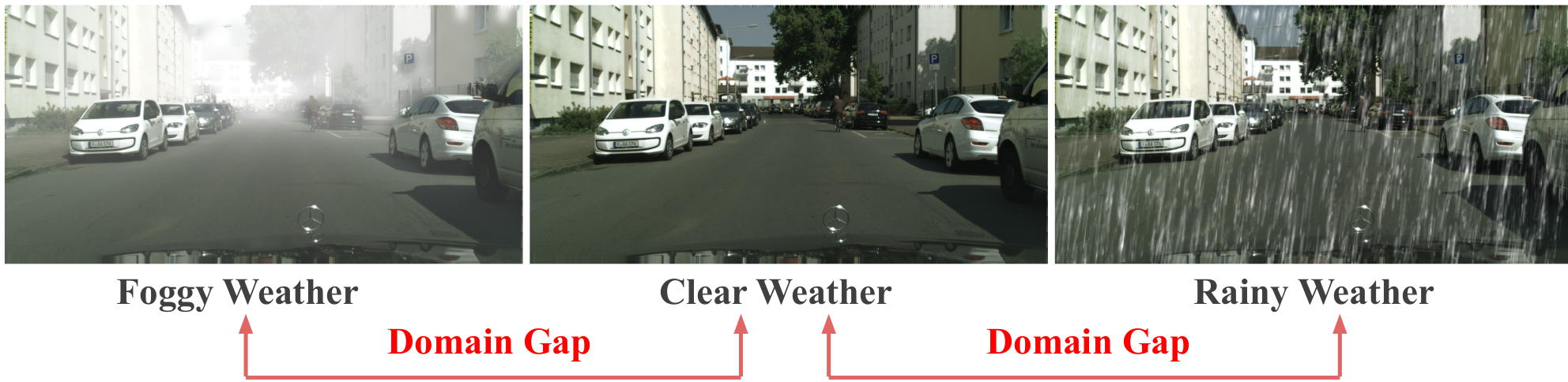
(a) The domain gap between different weather in the wild

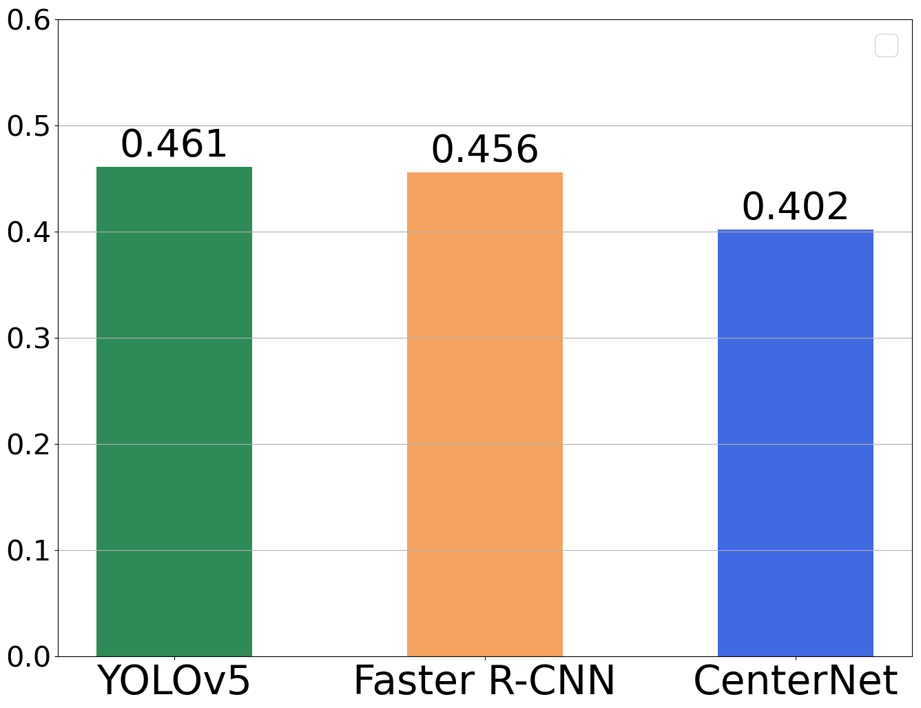
(b) Detection in clear weather

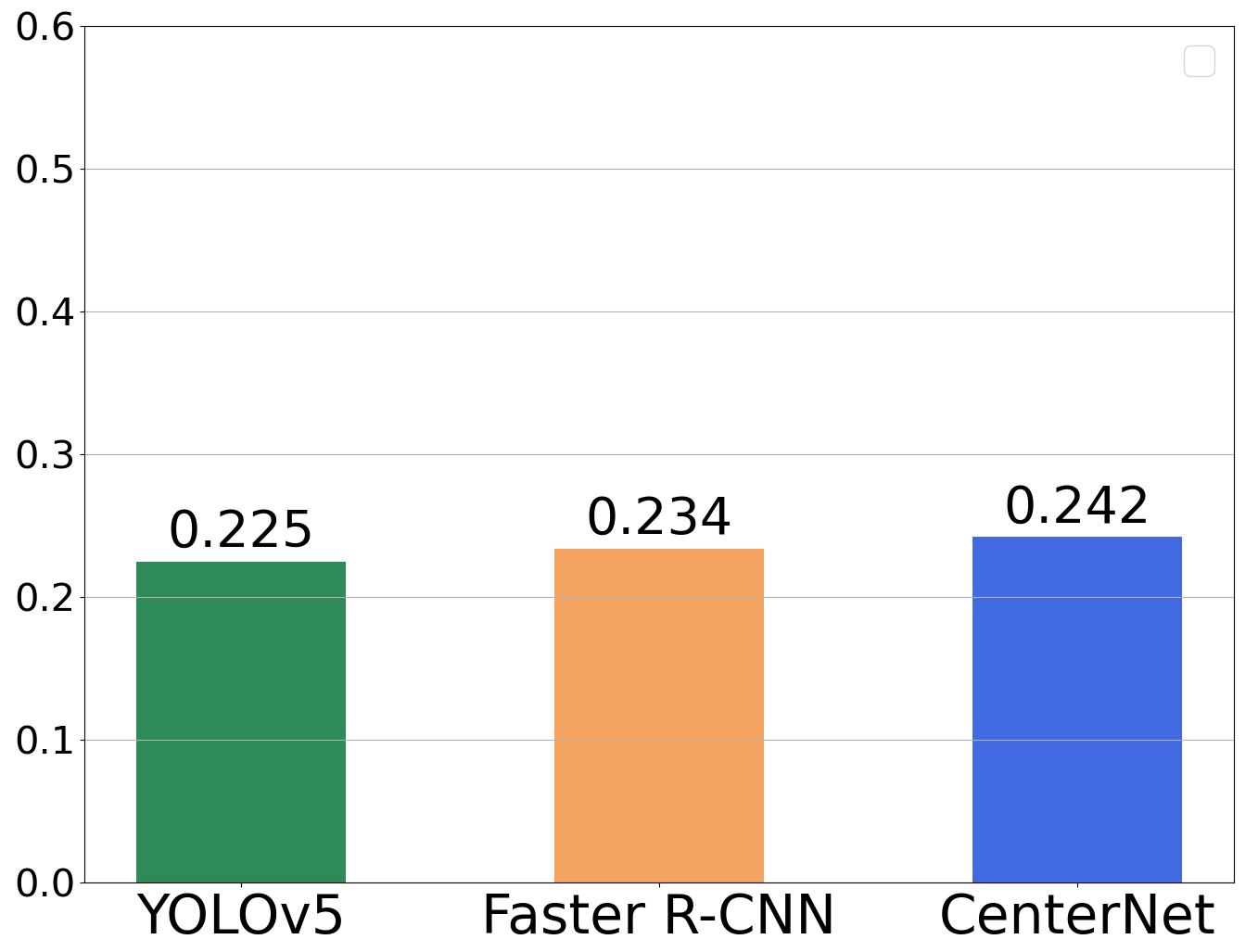
(c) Detection in foggy weather

Figure 1: Illustration of the weather domain gap (foggy and rainy) for autonomous driving and the detection performance drop because of the domain gap. Three deep learning models (YOLOv5 [19], Faster R-CNN [20], and CenterNet [21]) are all trained with the clear weather data of Cityscapes [22].

Thanks to the rapid advancements in deep learning, numerous object detection deep learning-based methods have achieved remarkable success in intelligent transportation systems. However, the impressive performance of these popular methods heavily relies on large-scale annotated data for supervised learning. Moreover, these methods make the assumption of consistent feature distributions between the training and testing data. In reality, this assumption may not hold true, especially in diverse weather conditions [23]. For example, as depicted in Fig. 1, CNN models such as YOLOv5 [19], Faster R-CNN [20], and CenterNet [21], trained on clear-weather data (source domain), exhibit accurate object detection performance under clear weather conditions (Fig. 1b). However, their performance significantly degrades under foggy weather conditions (Fig. 1c). This degradation can be attributed to the presence of a feature domain gap between different weather conditions, as illustrated in Fig. 1a. The model trained on the source domain is not familiar with the feature distribution in the target domain. Consequently, this paper aims to enhance object detection specifically in foggy and rainy weather conditions through domain adaptation-based transfer learning.

The objective of this paper is to reduce the domain gap between various weathers for enhanced object detection. To handle the domain shift problem (e.g. Clear$\to$Foggy and Clear$\to$Rainy), in this paper, we present a new domain adaptation framework that aims to enhance the robustness of object detection in foggy and rainy weather conditions. Our proposed framework follows an unsupervised setting, similar to previous works [24, 25, 26]. In this setting, we have well-labeled clear-weather images as the source domain, while the foggy and rainy weather images, which serve as the target domains, lack any annotations. This unsupervised setting is because that adverse weather images with labeling (manual annotating) are time-consuming and costly. Inspired by [24, 27], the proposed method aims to reduce the domain feature discrepancies in both image style and object appearance. To achieve domain-invariant features, we incorporate both image-level and object-level domain classifiers as components to facilitate domain adaptation in our CNN architecture. These classifiers are responsible for distinguishing between different domains. By employing an adversarial approach, our detection model learns to generate features that are invariant to domain variations, thereby confusing the domain classifiers. This adversarial design encourages the network to produce features that are agnostic to the specific weather conditions, leading to improved object detection performance in foggy and rainy weather scenarios.

Furthermore, we propose novel methodology for domain adaptation (DA). Current existing domain adaptation methods [24, 26, 28, 29, 27] might ignore: 1) the different challenging levels of various training samples, 2) the domain-level feature metric distance to the third related domain by only involving the source domain and target domain. This paper investigates the incorporation of hard example mining and an additional related domain to further strengthen the model’s ability to learn robust and transferable representations. We propose a novel Adversarial Gradient Reversal Layer (AdvGRL) and introduce an auxiliary domain through data augmentation. The AdvGRL is designed to perform adversarial mining on challenging examples, thereby improving the model’s ability to learn in challenging scenarios. Additionally, the auxiliary domain is leveraged to enforce a new domain-level metric regularization during the transfer learning process. In summary, the contributions of this paper can be summarized as follows:

• This paper proposes a novel unsupervised domain adaptation method to enhance the object detection for autonomous vehicle under foggy and rainy conditions, including the image-level and object-level adaptations.

• This paper proposes to perform adversarial mining for hard examples during domain adaptation to further improve the model’s transfer learning capabilities under challenging samples, which is accomplished by our proposed AdvGRL.

• This paper proposes a new domain-level metric regularization to improve transfer learning, i.e., the regularization constraint between source domain, added auxiliary domain, and target domain.

• This paper explores the intensive transfer learning experiments of clear$\rightarrow$foggy, clear$\rightarrow$rainy, cross-camera adaptation, and also carefully studies the different-intensity (small, medium, large) fog and rain adaptations.

II Related Work

II-A Detection for intelligent vehicles

The field of autonomous driving has made remarkable progress thanks to recent deep learning advancements [30, 31, 32]. Object detection, in particular, has emerged as one of the most actively researched areas in this field [33, 34]. In general, current object detection methods can be classified into two main categories: two-stage object detection methods and single-stage object detection methods. Two-stage methods typically consist of two main stages: region proposal generation and object classification/localization. The first process is region proposal, where potential object regions are identified within an image. The second process is object classification and localization refinement. In the beginning, R-CNN [35] introduced the concept of using selective search for generating region proposals and employing separate CNNs for each object prediction. Fast R-CNN [20] enhanced R-CNN by extracting object features directly from a shared CNN feature map. Faster R-CNN [20] enhanced the framework by introducing the Region Proposal Network (RPN) as a replacement for the selective search stage. This enhancement enabled more efficient and accurate region proposal generation. Single-stage detectors typically use a set of predefined anchor boxes or default boxes at different scales and aspect ratios to densely cover the image. Single-stage methods are typically faster in terms of inference speed compared to two-stage algorithms, but they may sacrifice some accuracy. Significant advancements in this category include the SSD series [36], YOLO series [37] , and RetinaNet [38]. Although these methods have achieved significant success in visual scenes with clear weather conditions, their direct application in autonomous driving scenarios is often limited due to the challenges posed by challenging real-world weather conditions.

II-B Detection for intelligent vehicles under foggy and rainy weather

In recent years, considerable research has been dedicated to addressing the challenges posed by various weather conditions encountered in autonomous driving scenarios. Researchers have generated various datasets [23, 39] and proposed numerous methods [40, 41, 42, 43, 44, 45] to improve object detection under adverse weather conditions. One notable example is the Foggy Cityscape dataset, which is a synthetic dataset created by applying fog simulation to the Cityscape dataset [23]. In the context of object detection research in rainy weather, several synthesized rainy datasets have been proposed [46, 44, 45]. [41] devised a fog simulation technique to augment existing real lidar datasets, thereby enhancing their quality and realism. The simulated foggy data offers valuable opportunities to enhance object detection methods that are specifically tailored for foggy weather conditions. For leveraging information from multiple sensors, [43] designed a network to integrate data from different sensors e.g., LiDAR, camera, and radar. [42] proposed a method that exploits both LiDAR and radar signals to obtain object proposals. The features extracted from the regions of interest in both sensors are fused together to improve the performance of object detection. However, these mentioned methods often rely on input data from different types of sensors other than the camera alone, which may not be applicable to all autonomous driving vehicles. Therefore, the objective of this work is to develop a DA network by utilizing only camera-sensor data as input.

II-C Object Detection via Domain Adaptation

Domain adaptation is effective in reducing the distribution discrepancy between different domains, enabling models trained on a labeled source domain to be applicable to an unlabeled target domain. There has been a growing interest in addressing domain adaptation for object detection [24, 47, 48, 49, 50, 51, 52, 27] in recent years. Several studies [24, 53, 48, 52, 27] have explored the alignment of features from different domains to achieve DA object detectors. A DA Faster R-CNN framework [24] was proposed to reduces the domain gap at both the image level and instance level. He et al. [53] proposed a MAF network that aligns domain features and proposal features hierarchically to minimize domain distribution disparity. In addition to feature alignment, image style transfer approaches [33, 47, 54, 55] are utilized to address the challenge of DA. An image translation module [33] was utilized to convert images from the source domain to the target domain. They then trained the object detector using adversarial training on the target domain. [54] adopted a progressive image translation strategy and introduced a weighted task loss during adversarial training to address image quality differences. Several previous methods [56, 57, 58, 59] have also proposed complex architectures for domain adaptation in object detection. Feature Pyramid Networks (FPN) was utilized to incorporate pixel-level and category-level adaptation for object detection [56] . In order to incorporate the uncertainty of unlabeled target data, [58] introduced an uncertainty-guided self-training mechanism, which leverages a Probabilistic Teacher and Focal Loss. Different with these methods, our approach does not introduce additional learnable parameters to the Faster R-CNN. Instead, we utilize an AdvGRL and a Domain-level Metric Regularization based on triplet loss. A key difference between our method and previous domain adaptation approaches lies in the treatment of training samples. While existing methods often assume that training samples are at the same challenging level, our approach introduces the AdvGRL for adversarial hard example mining, specifically targeting the improvement of transfer learning performance. Additionally, to mitigate overfitting and improve domain adaptation, an auxiliary domain is generated and incorporated to domain-level metric regularization.

III Methodology

This section introduces the overall network architecture, each detailed component, loss functions of our proposed method.

III-A Network Architecture

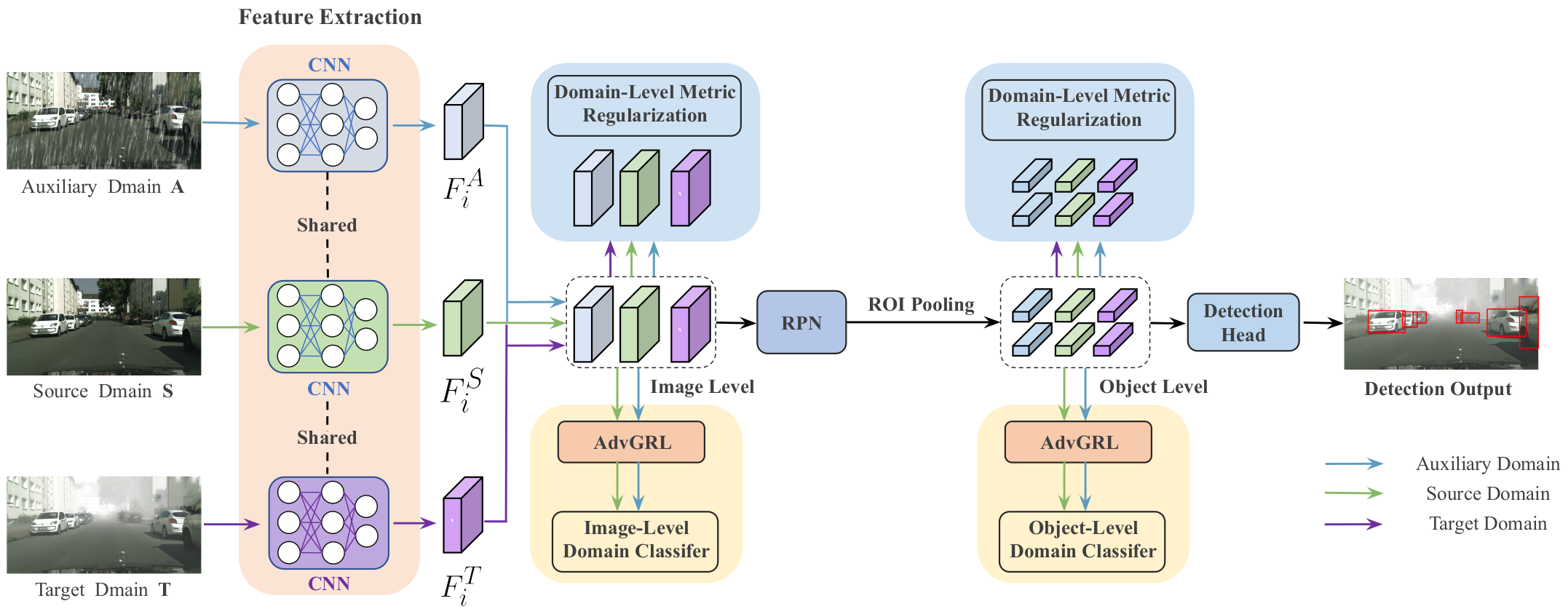
Figure 2: The architecture of the proposed domain adaptation based enhanced detection for intelligent vehicles in foggy and rainy weather. It is recommended to view this figure in color.

As shown in Fig. 2, our proposed network follows the pipeline of Faster R-CNN. In the first step, we involve a CNN backbone to extract the image-level features from input images. These features are then fed into the Region Proposal Network to produce region proposals. The next stage involves the ROI pooling, both the image-level features and the object proposals are as input to obtain object-level features. Finally, we apply a detection head for the object-level features to make the final outputs. To enhance the framework of Faster R-CNN for domain adaptation, we incorporate two additional domain adaptation modules: image-level and object-level modules. Both of them utilize a novel AdvGRL in conjunction with the domain classifier. By combining these modules, we are able to extract domain-invariant features and effectively perform adversarial hard example mining. Additionally, an auxiliary domain is introduced to enforce a new domain-level metric regularization. During training, source, target, and auxiliary domains, are simultaneously utilized.

III-B Image-level based Adaptation

The image-level domain representation is derived from the feature extraction process of the backbone network, encompassing valuable global information such as style, scale, and illumination. These factors have the potential to greatly influence the performance of the object detection task [24]. To address this, we incorporate a domain classifier, which aims to classify the domains of the extracted image-level features and promote global alignment at the image level. The domain classifier is implemented as two simple convolutional layers. It takes the image-level features as input and produces a prediction to identify the feature domain. A BCE loss is employed for the domain classifier as follows:

$$L_{img}=-\sum_{i=1}^{N}[G_{i}{\rm log}P_{i}+(1-G_{i}){\rm log}(1-P_{i})],$$ (1)

where $i\in\{1,...,N\}$ represents the $N$ training images, the ground truth domain label of the $i$-th training image is denoted as $G_{i}\in\{1,0\}$, where $G_{i}$ takes a value of 1 or 0 to represent the source and target domains, respectively. The prediction of the domain classifier for the $i$-th training image is denoted as $P_{i}$.

III-C Object-level based Adaptation

Besides the global differences at the image level, objects within different domains may exhibit variations in terms of appearance, size, color, and other characteristics. To address this, Each region proposal generated by the ROI Pooling layer is considered as a potential object of interest. After obtaining the object-level domain representation via ROI pooling, we introduce an object-level domain classifier to discern the origin of the local features, which is implemented by three fully-connected layers. The objective of the object-level domain classifier is to align the distribution of object-level features across different domains. Similar to the image-level domain classifier, we utilize the BCE loss to train our object-level domain classifier:

$$L_{obj}=-\sum_{i=1}^{N}\sum_{j=1}^{M}[G_{i,j}{\rm log}P_{i,j}+(1-G_{i,j}){\rm log}(1-P_{i,j})],$$ (2)

where $j\in\{1,...,M\}$ is the $j$-th predicted object in the $i$-th image, $P_{i,j}$ is the prediction of the object-level domain classifier for the $j$-th region proposal in the $i$-th image, The corresponding binary ground-truth label for the source and target domains is denoted as $G_{i,j}$.

III-D Adversarial Gradient Reversal Layer

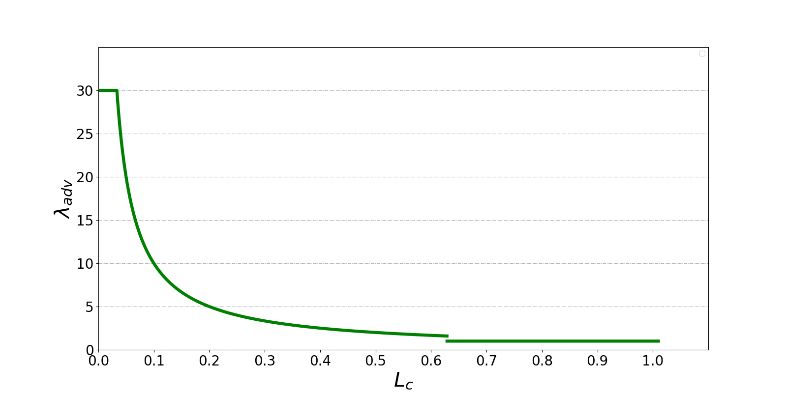
Figure 3: Illustration of the AdvGRL based hard training example mining. We assign larger responses to harder training examples with lower domain classifier loss ($L_{c}$) values. In this paper, we set $\lambda_{0}=1$ and $\beta=30$.

In this section, we will begin by providing a brief overview of the original Gradient Reversal Layer (GRL), which serves as the foundation for our proposed Adversarial Gradient Reversal Layer (AdvGRL).

The original GRL was initially developed for unsupervised domain adaptation in image classification tasks [60]. During forward propagation, the GRL leaves the input unchanged. However, during back-propagation, the gradient is reversed by multiplying it by a negative scalar before propagating it to the preceding layers of the base network. This reversal of gradients serves as a mechanism to confuse the domain classifier. Like this, by reversing the gradient during back-propagation, the GRL encourages the base network to learn domain-invariant features, enabling DA. The forward propagation of GRL is defined as:

$$R_{\lambda}({\mathbf{v}})={\mathbf{v}},$$ (3)

where ${\mathbf{v}}$ represents an input feature vector, and $R_{\lambda}$ represents the forward function performed by GRL. Back-propagation of GRL is defined as:

$$\frac{dR_{\lambda}}{d{\mathbf{v}}}=-\lambda\mathbf{I},$$ (4)

where $\mathbf{I}$ is an identity matrix and $-\lambda$ is a negative scalar.

In the original GRL, a constant or varying value of $-\lambda$ is utilized, which is determined by the training iterations, as described in [60]. However, this approach overlooks the fact that different training samples may exhibit varying levels of challenge during transfer learning. To address this limitation, this paper introduces a novel AdvGRL that incorporates adversarial mining for hard example. This is achieved by replacing the parameter $\lambda$ with a new parameter $\lambda_{adv}$ in Eq. (4) of GRL, resulting in the proposed AdvGRL. Notably, the value of $\lambda_{adv}$ is determined as follows:

$$\lambda_{adv}=\left\{\begin{aligned} &{\rm min}(\frac{\lambda_{0}}{L_{c}},\beta),\qquad&L_{c}<\alpha\\ &\lambda_{0},\qquad&{\rm otherwise},\end{aligned}\right.$$ (5)

where $L_{c}$ represents the loss of the domain classifier. $\alpha$ is a hardness threshold used to determine the difficulty level of the training sample. $\beta$ is the overflow threshold implemented to prevent the generation of excessive gradients during back-propagation. In our experiment, we set $\lambda_{0}=1$ as a fixed parameter. Namely, when the domain classifier’s loss $L_{c}$ is smaller, it indicates that the training sample’s domain can be more easily identified by the classifier. In this case, the features associated with this sample are not the desired domain-invariant features, making it a more difficult example for domain adaptation. The relationship between $\lambda_{adv}$ and $L_{c}$ is visualized in Fig. 3.

Ous proposed AdvGRL serves two main purposes. 1) It utilizes the concept of gradient reversal during back-propagation to confuse the domain classifier, thereby promoting the generation of domain-invariant features. 2) AdvGRL enables adversarial mining for hard examples, meaning that it selectively focuses on challenging examples that contribute to the model’s generalization. Fig. 2 illustrates the utilization of the AdvGRL in both the image-level and object-level DA modules.

III-E Domain-level Metric Learning based Regularization

A common transfer learning approach in many existing DA methods is to prioritize the transfer of features from a source domain $S$ to a target domain $T$. Hence, they often overlook the potential advantages that a third related domain can offer. To explore the potential advantages of incorporating a third related domain, we introduce an auxiliary domain for domain-level metric regularization that complements the source domain $S$. We leverage advanced data augmentation techniques to create this auxiliary domain $A$, which is particularly useful in autonomous driving scenarios where training data needs to be synthesized for different weather conditions based on existing clear-weather data. As a result, in our proposed architecture (as shown in Fig. 2), the source, auxiliary, and target domain images are regarded as aligned images, ensuring the enforcement of domain-level metric constraints across these three distinct domains.

The global image-level features of the $i$-th training image for the source ($S$), auxiliary ($A$), and target ($T$) domains are defined as $F_{i}^{S}$, $F_{i}^{A}$, and $F_{i}^{T}$, respectively. Our goal is to reduce the domain gap between $S$ and $T$ and ensure that the feature metric distance between $F_{i}^{S}$ and $F_{i}^{T}$ is closer compared to the distance between $F_{i}^{S}$ and $F_{i}^{A}$. This can be expressed as:

$$d(F_{i}^{S},F_{i}^{T})<d(F_{i}^{S},F_{i}^{A}),$$ (6)

where the metric distance between the corresponding features is denoted as $d(,)$. To implement this constraint, we can use a triplet structure where $F_{i}^{S}$, $F_{i}^{T}$, and $F_{i}^{A}$ are treated as the anchor, positive, and negative, respectively. Therefore, the image-level constraint in Eq. (6) can be equivalently expressed as minimizing the image-level triplet loss:

$$L^{R}_{img}={\rm max}(d(F_{i}^{S},F_{i}^{T})-d(F_{i}^{S},F_{i}^{A})+\delta,0),$$ (7)

where the margin constraint is denoted as $\delta$, and in our experiments, $\delta$ is set as $1.0$.

Equivalently, the $i$-th training image’s $j$-th object-level features of $S$, $A$, and $T$ are defined as $f_{i,j}^{S}$, $f_{i,j}^{A}$, and $f_{i,j}^{T}$ respectively. To apply our proposed metric regularization to the object-level features, we further minimize the object-level triplet loss:

$$L^{R}_{obj}={\rm max}(d(f_{i,j}^{S},f_{i,j}^{T})-d(f_{i,j}^{S},f_{i,j}^{A})+\delta,0).$$ (8)

III-F Training Loss

The overall training loss of the proposed network consists of several individual components. It can be expressed as follows:

$$L=\gamma*(L_{img}+L_{obj}+L^{R}_{img}+L^{R}_{obj})+L_{cls}+L_{reg},$$ (9)

where $L_{cls}$ and $L_{reg}$ represent the loss of classification and the loss of regression respectively. A weight parameter $\gamma$ is introduced to balance the Faster R-CNN loss and the domain adaptation loss, which is set as $0.1$. During the training phase, the network can be trained in an end-to-end manner utilizing a standard SGD algorithm. During the testing phase, the object detection can be performed using the Faster R-CNN with the trained adapted weights.

III-G General Domain Adaptive Detection with Proposed Method

Our proposed method is designed to be versatile and adaptable to various domain adaptive object detection scenarios. Specifically, when dealing with scenarios where the target domain images are generated from the source domain with pixel-to-pixel correspondence, such as the Clear Cityscapes$\longrightarrow$Foggy Cityscapes, our method can be directly applied without any modifications. To utilize our method with unaligned datasets in real-world scenarios, where the target and source domains lack strict correspondence, such as the Cityscapes$\longrightarrow$KITTI, we can remove the $L^{R}_{obj}$ loss, which eliminates the requirement for object alignment during training. This allows our method to be applied directly without the need for object-level alignment.

IV Experiments

IV-A Benchmark

Cityscapes [22]: It is a widely used computer vision dataset that focuses on urban street scenes. There are 2,975 training set and 500 validation set from 27 different cities. The dataset includes annotations for $8$ different categories. All images in the Cityscapes dataset are 3-channel $1024\times 2048$ images.

Foggy Cityscapes [23]: It is a public benchmark dataset created by simulating different intensity levels of fog on the original Cityscapes images. This dataset uses a depth map and a physical model [23] to generate three levels of simulated fog.

Rainy Cityscapes: We synthesize a rainy-weather dataset named as Rainy Cityscapes in this paper from the original Cityscapes dataset. Specifically, the training set of 3,475 images and the validation set of 500 images from Cityscapes are used to create the Rainy Cityscapes dataset by utilizing a novel data augmentation method called RainMix [61, 62]. To generate rainy Cityscapes images, we utilize a combination of techniques. First, we randomly sample a rain map from a publicly dataset of real rain streaks [63]. Next, we apply random transformations to the rain map using the RainMix technique. These transformations include rotation, zooming, translation, and shearing, which are randomly sampled and combined. Lastly, the rain maps after transformation are merged with the original source domain images, resulting in the generation of rainy Cityscapes images. An example illustrating this process can be seen in Figure 4.

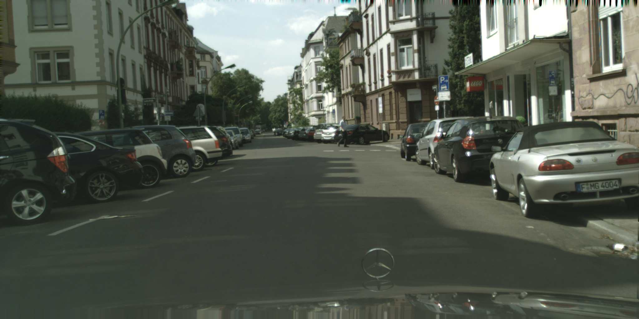
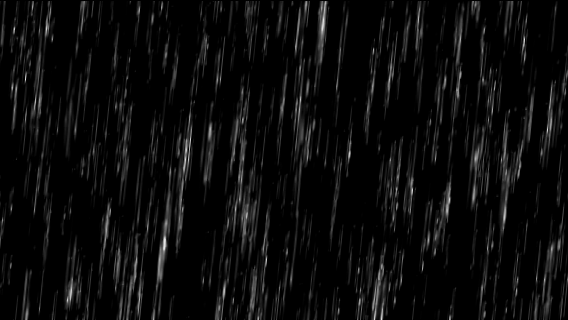
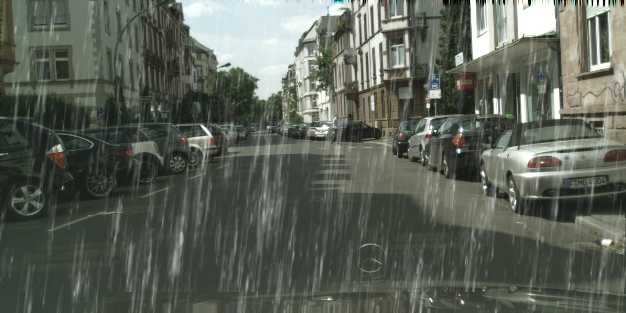
Figure 4: Illustration of synthesizing Rainy Cityscapes from the Cityscapes data: (a) the original image from Cityscapes [22], (b) rain map generated by RainMix [61], (c) synthesized rainy image.

Intensity levels of fog/rain: For the Foggy Cityscapes and Rainy Cityscapes datasets, their number of images, resolution, and annotations are identical to those of Clear Cityscapes dataset. Based on physical model of [23], the different intensity levels of fog could be synthesized on the Foggy Cityscapes dataset. After obtaining the rain maps by RainMix [61], the intensity of rain maps could be further processed with different erosion levels. In these two ways, the different fog and rain levels (small, medium, large) can be synthesized, as shown in Fig. 5. Following the setting  [24, 52, 27], the images with the highest intensity level of fog/rain are selected as the target domain for model training. The models trained with highest intensity level will be then used to test the performance on the validation sets of different fog/rain intensity levels (small, medium, large).

IV-B Experimental Setting

TABLE I: Adaptation from Clear to Foggy: Cityscapes$\rightarrow$Foggy Cityscapes experiment.

Methodologies	$C_{bus}$	$C_{bicycle}$	$C_{car}$	$C_{mcycle}$	$C_{person}$	$C_{rider}$	$C_{train}$	$C_{truck}$	mAP
MCAR-ECCV’2020 [49]	44.1	36.6	43.9	37.4	32.0	42.1	43.4	31.3	38.8
MTOR-CVPR-2019 [64]	38.6	35.6	44.0	28.3	30.6	41.4	40.6	21.9	35.1
DA-Faster-CVPR’2018 [24]	49.8	39.0	53.0	28.9	35.7	45.2	45.4	30.9	41.0
GPA-CVPR’2020 [52]	45.7	38.7	54.1	32.4	32.9	46.7	41.1	24.7	39.5
RPN-PR-CVPR’2021 [51]	43.6	36.8	50.5	29.7	33.3	45.6	42.0	30.4	39.0
UaDAN-TMM’2021 [27]	49.4	38.9	53.6	32.3	36.5	46.1	42.7	28.9	41.1
HTCN-CVPR’2020 [65]	47.4	37.1	47.9	32.3	33.2	47.5	40.9	31.6	39.8
SAPN-ECCV’2020 [66]	46.8	40.7	59.8	30.4	40.8	46.7	37.5	24.3	40.9
MeGA-CDA-CVPR’2021 [67]	49.2	39.0	52.4	34.5	37.7	49.0	46.9	25.4	41.8
UMT-CVPR2021 [68]	56.6	37.3	48.6	30.4	33.0	46.7	46.8	34.1	41.7
SCAN-AAAI’2022 [69]	48.6	37.3	57.3	31.0	41.7	43.9	48.7	28.7	42.1
ParaUDA-TITS’2022 [70]	48.3	37.6	52.5	33.5	36.7	46.7	45.9	32.3	41.7
ConfMix-WACV’2023 [71]	45.8	33.5	62.6	28.6	45.0	43.4	40.0	27.3	40.8
SDAYOLO-TIV’2023 [72]	40.5	37.3	61.9	24.4	42.6	42.1	39.5	23.5	39.0
MS-DAYOLO-TIP’2023 [73]	51.0	36.0	56.5	27.5	39.6	46.5	45.9	28.9	41.5
Ours w/o Auxiliary Domain	48.4	36.7	53.5	26.1	36.1	45.9	39.1	29.3	40.2
Ours	51.2	39.1	54.3	31.6	36.5	46.7	48.7	30.3	42.3
Oracle	49.9	45.8	65.2	39.6	46.5	51.3	34.2	32.6	45.6

TABLE II: Adaptation from Clear to Rainy: Cityscapes$\rightarrow$Rainy Cityscapes experiment.

Methodologies	$C_{bus}$	$C_{bicycle}$	$C_{car}$	$C_{mcycle}$	$C_{person}$	$C_{rider}$	$C_{train}$	$C_{truck}$	mAP
Faster R-CNN (source only)	46.3	26.0	54.8	25.8	34.7	35.9	26.9	23.9	34.3
DA-Faster-CVPR’2018 [24]	54.6	33.8	59.6	32.4	38.2	41.6	42.9	33.8	42.1
MS-DAYOLO-TIP’2023 [73]	60.3	34.4	67.7	31.9	47.2	47.4	31.9	30.7	44.0
Ours w/o Auxiliary Domain	55.5	35.3	60.0	32.8	38.3	22.1	49.3	33.1	43.4
Ours	60.0	35.3	60.6	33.8	38.8	42.9	52.4	36.3	45.0
Oracle	58.5	35.3	66.9	35.7	47.5	50.9	37.4	40.5	46.6

Dataset setting: We conducted two main experiments in this paper: 1) Clear to Foggy Adaptation, denoted as Clear Cityscapes$\rightarrow$Foggy Cityscapes, the labeled training set of Clear Cityscapes [22] and the unlabeled training set of Foggy Cityscapes [23] are used as the source and target domains during training, respectively. Subsequently, the trained model was evaluated Foggy Cityscapes validation set to report the performance. Rainy Cityscapes training set is used as the Auxiliary Domain $A$ in this Clear to Foggy Adaptation experiment. 2) Clear to Rainy Adaptation, denoted as the Clear Cityscapes$\rightarrow$Rainy Cityscapes, where the labeled training set of Clear Cityscapes [22] and the unlabeled training set of Rainy Cityscapes are used as the source and target domains during training, respectively. Then the trained model was evaluated on Rainy Cityscapes validation set to report the performance. Foggy Cityscapes training set is used as the Auxiliary Domain $A$ in this Clear to Rainy Adaptation experiment. Additionally, we analyzed the transfer learning performance on different intensity levels of fog and rain (small, medium, and large).

Training setting: We utilize ResNet-50 as the backbone for the Faster R-CNN [20]. Following in [24, 20], during training, We utilize back-propagation and stochastic gradient descent (SGD) to optimize all the deep learning methods in our approach. The initial learning rate of $0.01$ for $50,000$ iterations is used in all model training. Afterward, the learning rate is reduced to $0.001$ and training continues for an additional $20,000$ iterations. Weight decay is set as $0.0005$ and momentum is set as $0.9$ for all experiments. Each training batch consists of three images from source, target, and auxiliary domains respectively. For comparison purposes, we set the $\lambda$ value in the original GRL (Equation (4)) to $1$. In the AdvGRL (Equation (5)), the hardness threshold $\alpha$ is set to $0.63$, which is computed by averaging the parameters in Equation (1) with setting ($P_{i}=0.7,G_{i}=1$ and $P_{i}=0.3,G_{i}=0$).

Evaluation metrics: We calculate the Average Precision for each category and the mean Average Precision across all categories using an Intersection over Union threshold of $0.5$.

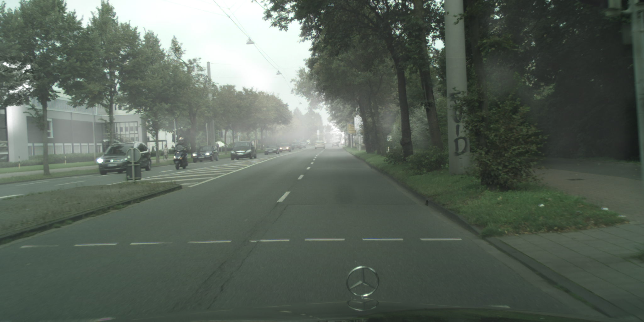
(a) Small Fog

(b) Medium Fog

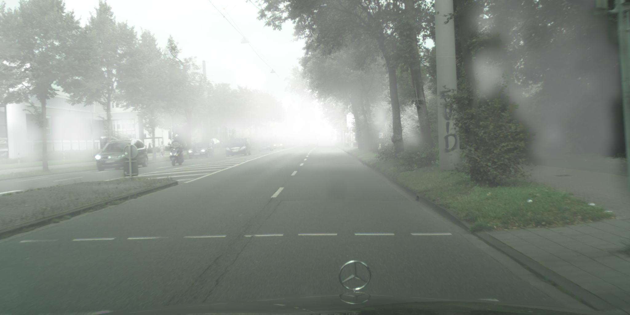
(c) Large Fog

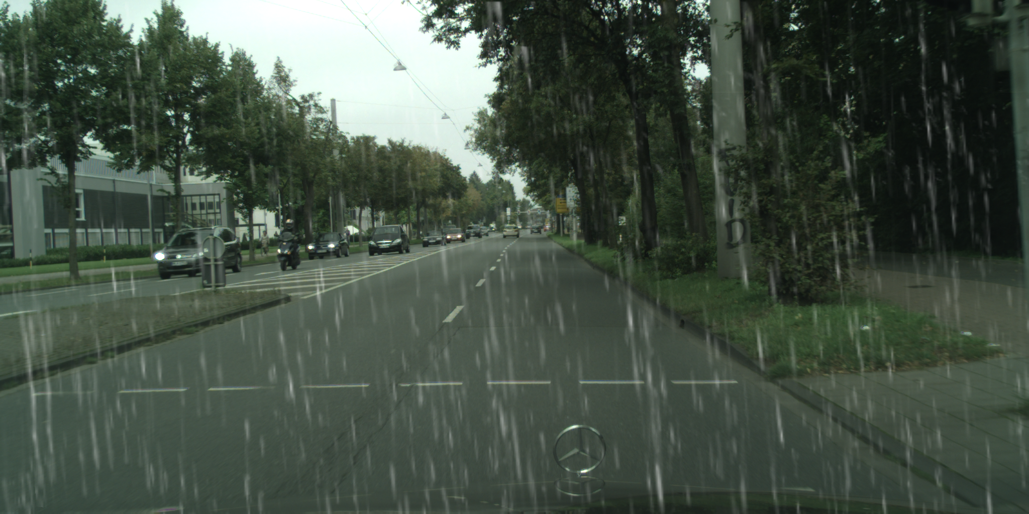
(d) Small Rain

(e) Medium Rain

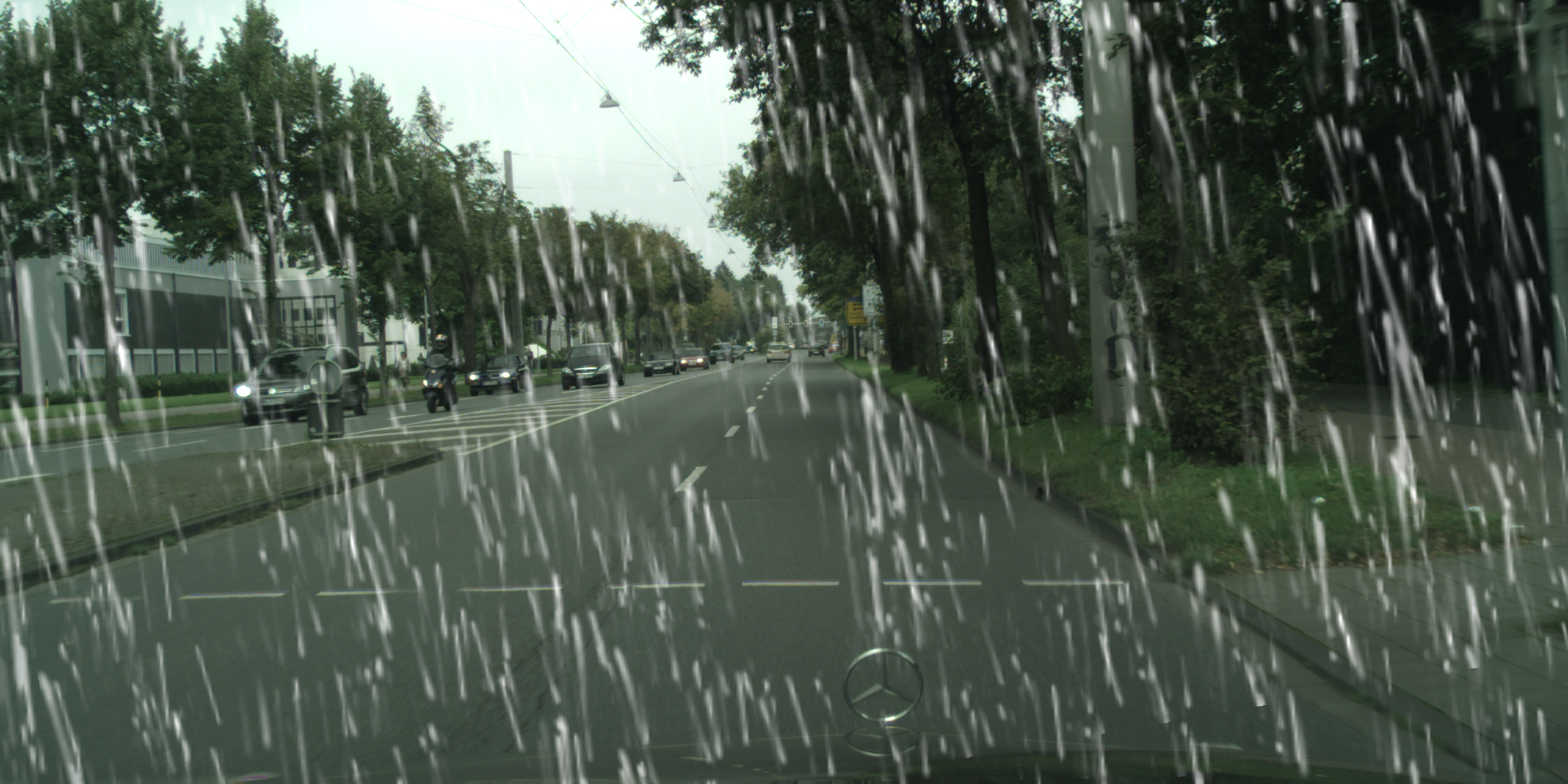
(f) Large Rain

Figure 5: Sample visualization results for the Foggy Cityscapes and Rainy Cityscapes validation sets with different intensity levels.

IV-C Adaptation from Clear to Foggy

Table I presents the results of our experiments on weather adaptation from clear to foggy. In comparison to other DA methods, our proposed DA method achieves the highest performance on Foggy Cityscape, with a mAP of $42.3\%$, which outperforms the second-best method SCAN [69] by a margin of $0.2\%$ in terms of mAP improvement. The proposed method effectively reduces the domain gap across various categories, e.g., bus got $51.2\%$ and bicycle got $39.1\%$ as the second best performance, and train got $48.7\%$ as the best performance in AP, which is the highlight in Table I. While UMT got $56.6\%$ in bus and $34.1\%$ in truck, SAPN got $40.7\%$ in bicycle, MeGA-CDA got $49.0\%$ in rider, our proposed DA method exhibits similar performance across them with only minor differences. However, our proposed DA method achieves the highest overall mAP detection performance on Foggy Cityscapes among the recent DA methods.

TABLE III: Ablation study of components on the experiments of Cityscapes$\rightarrow$Foggy Cityscapes and Cityscapes$\rightarrow$Rainy Cityscapes.

Methods	Img	Obj	AdvGRL	Reg	Foggy mAP	Rainy mAP
Source only					23.41	34.35
img w/ GRL	✓				38.10	36.41
obj w/ GRL		✓			38.02	37.92
img+obj w/ GRL (Baseline)	✓	✓			38.43	41.02
img+obj w/AdvGRL	✓	✓	✓		40.23	43.44
img+obj+ Reg w/ GRL	✓	✓		✓	41.97	44.44
img+obj+Reg w/ AdvGRL	✓	✓	✓	✓	42.34	45.07

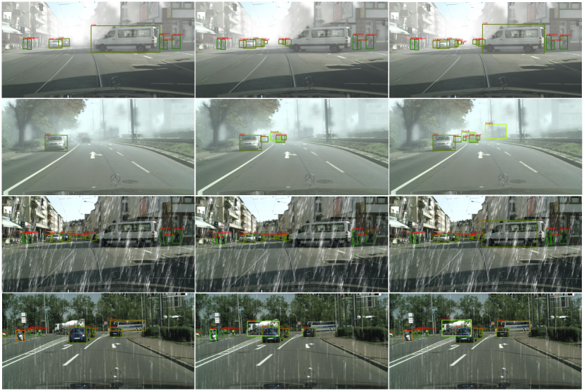
Figure 6: Visualization of the qualitative detection on Foggy/Rainy Cityscapes (validation sets). First column (Source only): original Faster R-CNN w/ DA, Second column (Baseline): Faster R-CNN with image-level and object-level adaptations w/ GRL, Third column: Proposed DA Method. Top: foggy weather, Bottom: rainy weather.

IV-D Adaptation from Clear to Rainy

In the Clear to Rainy adaptation, the only difference during training is the exchange of domains, where the unlabelled Rainy Cityscapes training set serves as the target domain, while the Foggy Cityscapes training set is used as the auxiliary domain. Table II presents the results of domain adaptation from clear to rainy weather. Due to the page limit, we choose the methods with the public available source code which perform very well in the Clear to Foggy Adaptation experiment as the comparison methods in this Clear to Rainy Adaptation experiment, i.e., DA-Faster [24], MS-DAYOLO [73]. Similar to the Clear to Foggy Adaptation, our proposed domain adaptation method got the best overall mAP (45.07%) detection performance on Rainy Cityscapes compared to the comparison methods.

IV-E Ablation Study of Components

We conduct an analysis of the individual proposed components of our DA object detection method. The experiments are conducted on the Cityscapes$\rightarrow$Foggy Cityscapes and Cityscapes$\rightarrow$Rainy Cityscapes tasks, using the ResNet-50 backbone. The results of the ablation study are presented in Table III. In the first row of the table, image-level and object-level adaptation modules are labels as ‘img’ and ‘obj’, respectively. ‘AdvGRL’ and ‘Reg’ indicate the proposed Adversarial GRL and domain-level metric regularization, respectively. The ‘img+obj+GRL’ configuration represents the Baseline model used in our experiments. We also evaluate two additional configurations: ‘img+obj+AdvGRL’ and ‘img+obj+AdvGRL+Reg’. Additionally, we include the ‘Source only’ configuration, which refers to the Faster R-CNN model trained solely on labeled source domain images without any DA methods. The ablation study presented in Table III provides clear evidence of the positive impact of each proposed component in the DA method for both foggy and rainy weather scenarios. Furthermore, we provide qualitative visualization of the object detection results in Fig. 6.

IV-F Adaptation of Different-intensity Fog and Rain

Moreover, both simulated Foggy and Rainy Cityscapes datasets contain three levels of intensity, namely Small, Medium, and Large as depicted in Fig. 5. Following the previous works [24, 52, 27], we only utilize the Large intensity level as the target domain during training for both fog and rain. After training, the trained models on the validation set of Rainy Cityscapes and Foggy Cityscapes with images of different intensity levels are evaluated. For the three intensity levels of fog and rain, as shown in Table IV, the ‘Baseline’ model after domain adaptation could get better detection performance compared to the ‘Source only’ without DA, while the Proposed Method could continue to further improve the performance compared to the ‘Baseline’ method. Alternatively, our proposed DA method could significantly mitigate the impact of fog and rain under Small, Medium, Large intensity levels.

TABLE IV: Adaptation of Different-intensity Fog and Rain: Cityscapes$\rightarrow$Foggy Cityscapes and Cityscapes$\rightarrow$Rainy Cityscapes experiments.

Foggy / Rainy	Methodologies	$C_{bus}$	$C_{bicycle}$	$C_{car}$	$C_{mcycle}$	$C_{person}$	$C_{rider}$	$C_{train}$	$C_{truck}$	mAP
	Source only	27.1 / 46.3	28.3 / 26.0	32.8 / 54.8	18.4 / 25.8	28.6 / 34.7	32.2 / 35.9	4.9 / 26.9	14.7 / 23.9	23.4 / 34.3
	Baseline	45.4 / 49.5	36.7 / 32.6	53.5 / 58.3	26.0 / 31.4	36.1 / 36.1	45.9 / 41.4	37.1 / 43.4	26.3 / 35.1	38.4 / 41.0
Large	Proposed Method	51.2 / 60.0	39.1 / 35.3	54.3 / 60.6	31.6 / 33.8	36.5 / 38.8	46.7 / 42.9	48.7 / 52.4	30.3 / 36.3	42.3 / 45.0
	Source only	40.6 / 47.1	36.9 / 26.9	48.9 / 54.6	27.3 / 23.9	37.9 / 34.0	43.2 / 38.6	40.4 / 30.8	22.4 / 30.7	37.2 / 35.8
	Baseline	52.0 / 47.3	40.5 / 33.3	58.9 / 58.2	31.7 / 27.9	40.8 / 35.8	50.0 / 44.3	39.8 / 35.1	29.9 / 36.4	42.9 / 39.8
Medium	Proposed Method	52.6 / 58.8	42.6 / 37.1	59.3 / 60.0	32.1 / 30.9	41.2 / 38.6	47.5 / 45.1	48.8 / 41.0	32.5 / 39.7	44.6 / 43.9
	Source only	49.2 / 43.8	40.9 / 29.6	55.7 / 55.7	33.1 / 24.1	41.0 / 35.7	47.0 / 37.5	43.1 / 38.7	28.4 / 23.3	42.3 / 36.0
	Baseline	54.1 / 42.9	40.6 / 34.5	60.3 / 59.0	32.5 / 30.7	42.0 / 36.7	51.0 / 43.7	49.3 / 48.1	31.9 / 36.1	45.2 / 41.5
Small	Proposed Method	52.9 / 53.6	43.1 / 38.3	60.6 / 61.3	36.3 / 33.6	42.7 / 39.4	49.4 / 42.8	54.8 / 51.4	36.5 / 35.7	47.0 / 44.5

IV-G Adaptation of Cross Cameras

We conducted an experiment specifically targeting the real-world cross-camera adaptation for different autonomous driving datasets with varying camera settings. We applied our DA method for cross-camera adaptation i.e., Cityscapes dataset (source) $\rightarrow$ KITTI dataset (target). To accommodate the unaligned nature of the datasets, we simply removed the $L^{R}_{obj}$ term (Eq. 8) during the adaptation process. Following the previous work [24], we used the KITTI training set, consisting of 7,481 images as the target domain. Specifically, we evaluated the AP of the Car category on the target domain. Table V demonstrated the outstanding performance of our proposed DA method compared to recent comparison methods.

IV-H Feature Distribution Visualization via Adaptation

To investigate the capability of our proposed DA method to overcome the domain shift (clear weather $\rightarrow$ rainy/foggy weather), we visualize these domain feature distributions by utilizing t-SNE [74] before and after the domain adaptation in foggy and rainy weather. Fig. 7 obviously presents that our proposed DA method could align the feature distributions to bridge the domain gap (clear weather $\rightarrow$ rainy/foggy weather).

TABLE V: Adaptation of cross cameras on Cityscapes$\rightarrow$KITTI experiment.

Methodologies	Car AP
MAF-ICCV’2019 [53]	72.10
SWDA-CVPR’2019 [48]	71.00
ATF-ECCV’2020 [75]	73.50
ART-CVPR’2020 [29]	73.60
GPA-CVPR’2020 [52]	65.36
SGA-TMM’2021 [76]	72.02
UIT-ESwA’2022 [77]	73.70
ParaUDA-TITS’2022 [70]	72.20
IDF-TCSVT’2023 [78]	74.00
Ours	74.38

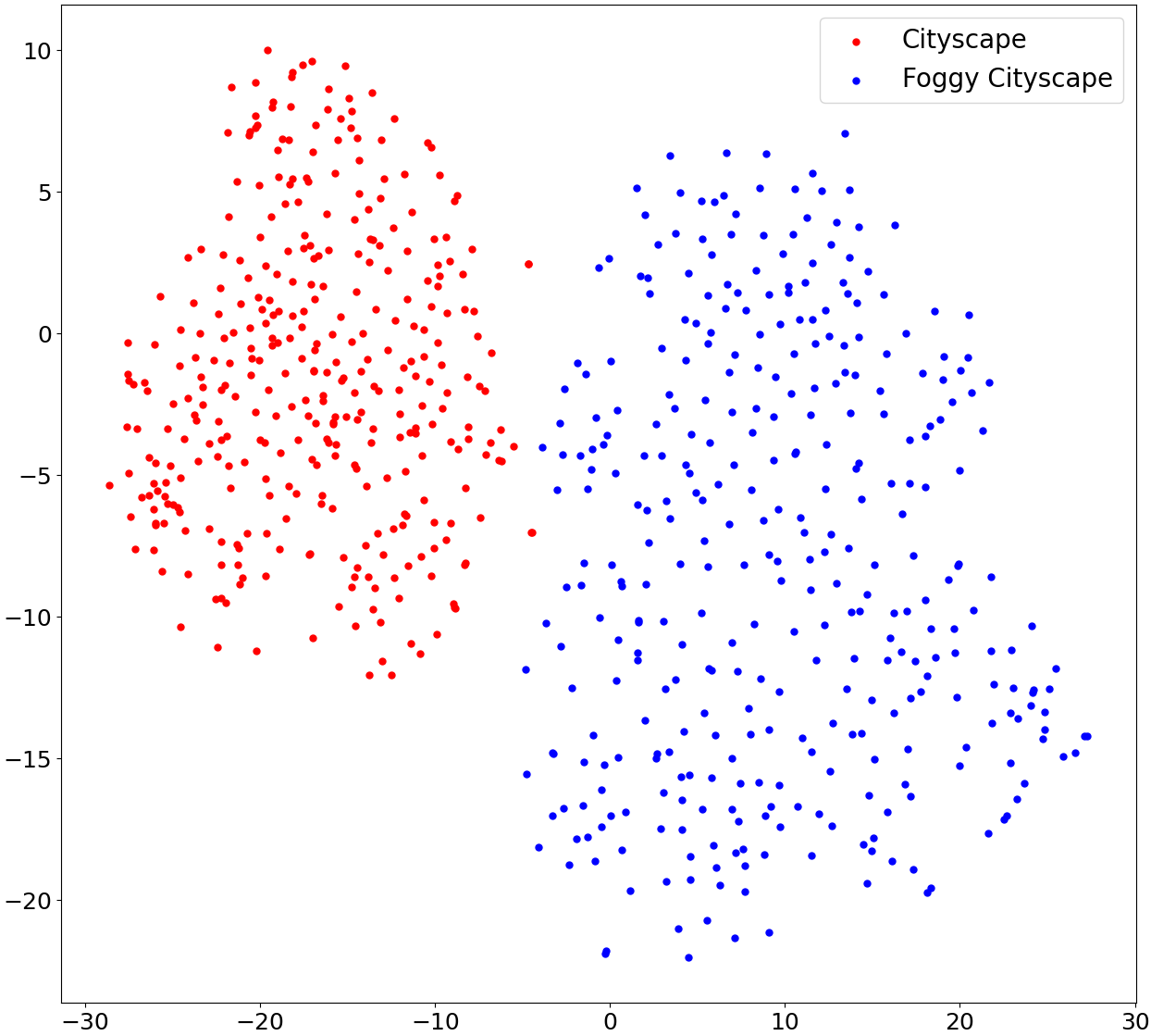
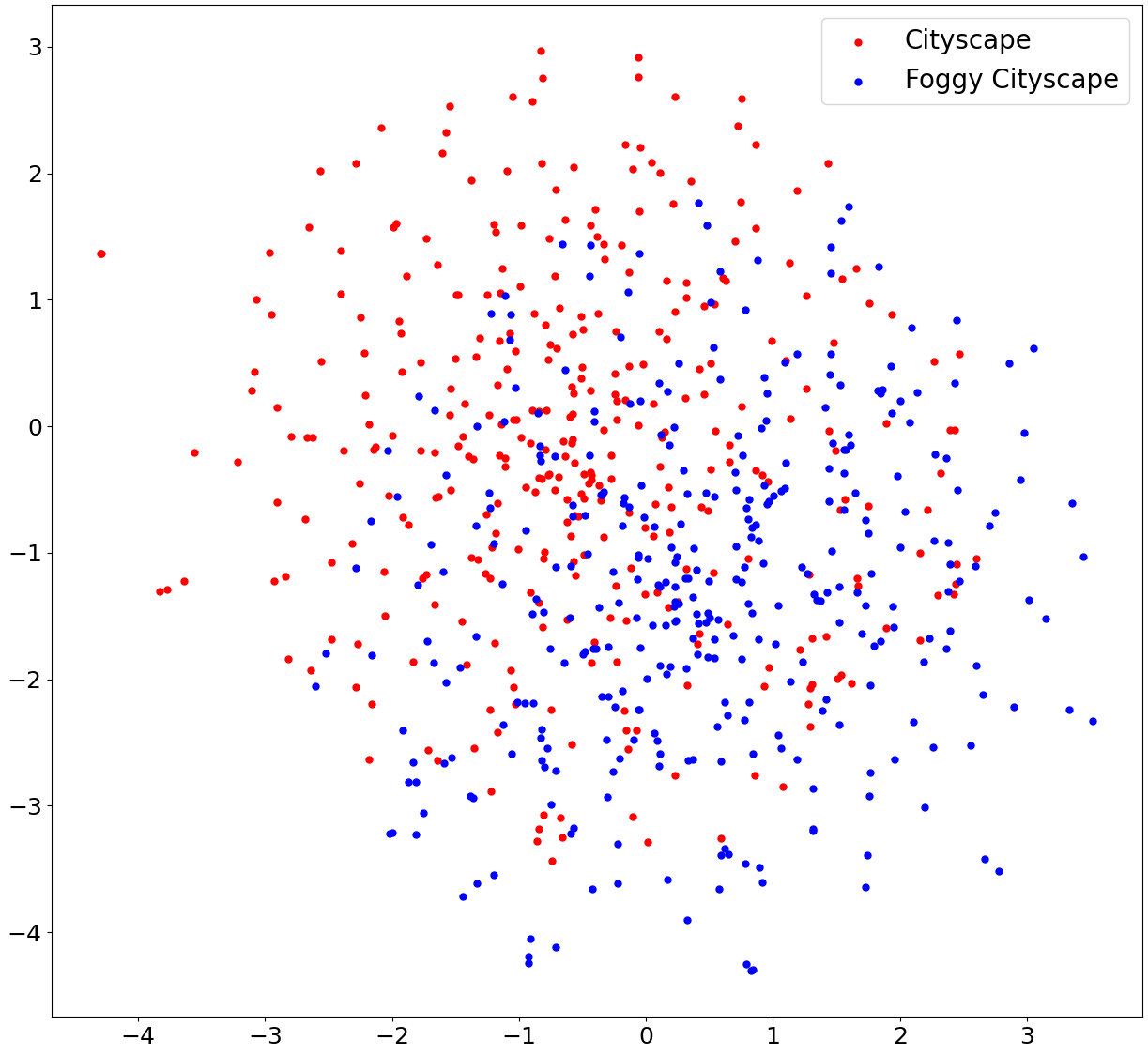
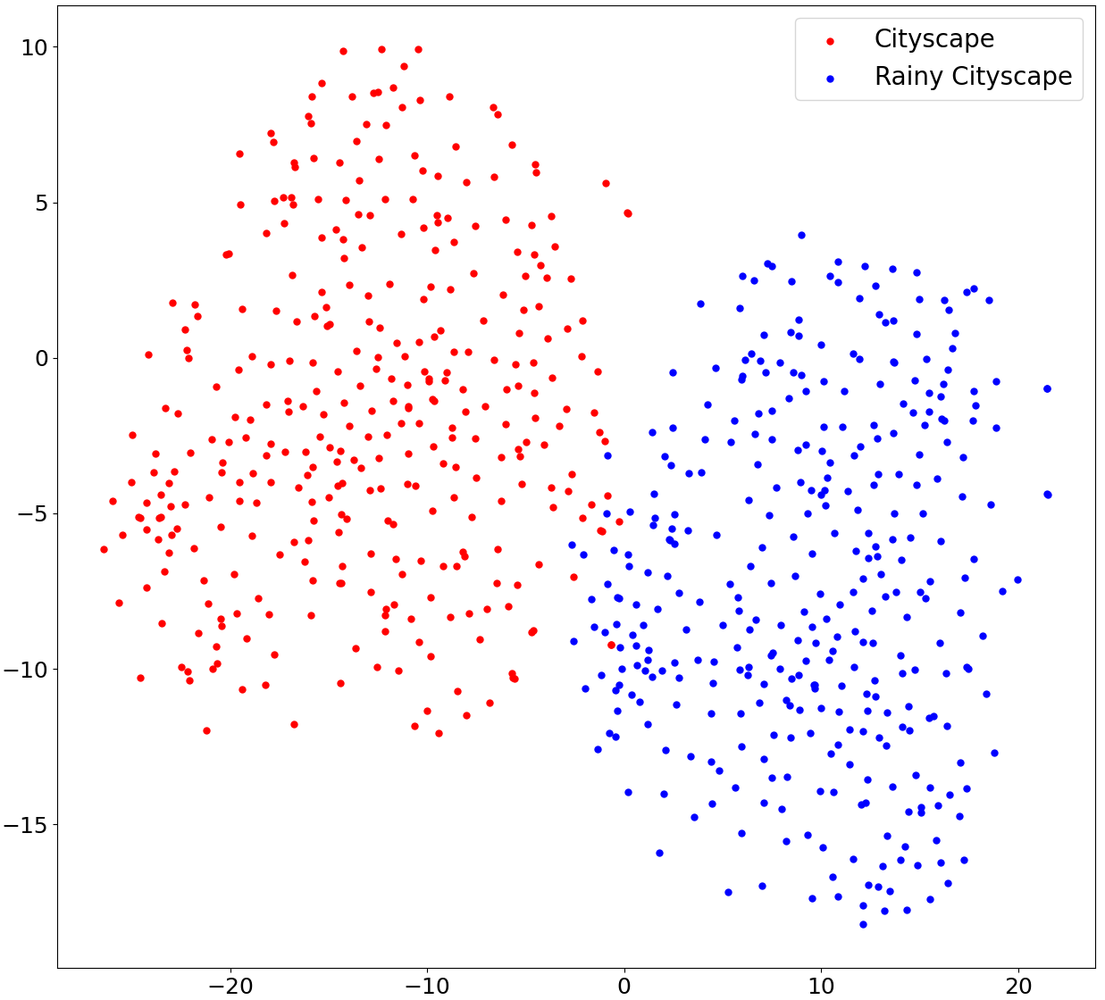
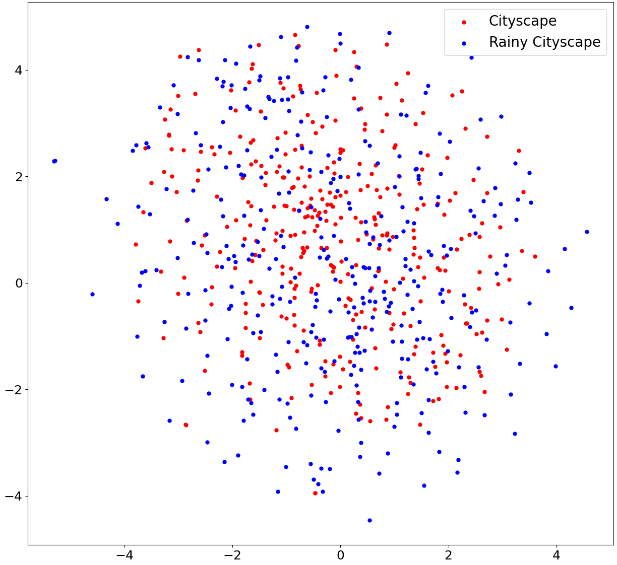
Figure 7: Feature distribution visualization by t-SNE [74] before and after domain adaptation. Clear to Foggy Adaptation: (a) original distribution before adaptation, (b) aligned distribution after the proposed adaptation. Clear to Rainy Adaptation: (c) original distribution before adaptation, (d) aligned distribution after the proposed adaptation. It is recommended to view this figure in color.

IV-I Experiments on Different Parameters

We analyze the detection performance on different hyper-parameters in Section III, .i.e, Eq.9 and Eq.5 for the Cityscapes$\rightarrow$Foggy Cityscapes case, and several hyper-parameters were investigated. First of all, $mAP_{\gamma}$ can be obtained $mAP_{0.1}=42.34,mAP_{0.01}=41.30,mAP_{0.001}=41.19$, where $\gamma$ represents loss balance weight in Eq. 9. Then, in the AdvGRL (Eq. 5), the $(\alpha,\beta)$, where $\beta$ represents the overflow threshold and $\alpha$ represents hardness threshold are set as (a) $(0.63,30)$, (b) $(0.63,10)$, (c) $(0.54,30)$, and (d) $(0.54,10)$, where $\alpha=0.54$ is obtained by averaging the values of Eq. 1 when $P_{i}=0.9,G_{i}=1$ and $P_{i}=0.1,G_{i}=0$. The corresponding detection mAP(s) are (a) 42.34, (b) 38.83, (c) 39.38, (d) 40.47, respectively.

IV-J Visualization of Hard Examples

By utilizing $\lambda_{adv}$ of the proposed AdvGRL, we can identify hard examples during the domain adaptation process. Fig.8 illustrates some of these hard examples. We compute the $L_{1}$ distance between the features $F^{S}_{i}$ and $F^{T}_{i}$ obtained from the backbone of Fig.2. This distance is used as an approximation of the example’s hardness ($ah$), where a smaller $ah$ indicates a harder example for transfer learning. Intuitively, when the fog covers a larger number of objects, as illustrated by the bounding-box regions in Fig. 8, the task becomes more challenging.

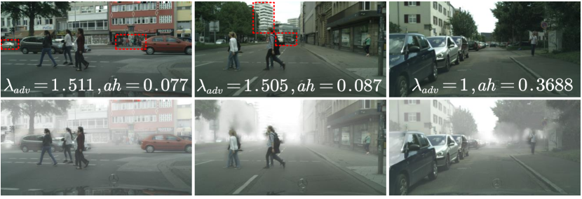
Figure 8: Visualization of hard examples mined by AdvGRL. Two mined hard examples and one easy example are shown from left to right.

IV-K Experiments on Pre-trained Models and Domain Randomization

Pre-trained Models: In the experiment of Cityscapes$\rightarrow$Foggy Cityscapes, our proposed DA method utilizes a pre-trained Faster R-CNN as an initialization, and achieves a detection mean Average Precision (mAP) of 41.3, compared to a mAP of 42.3 achieved when our method is initialized without the pre-trained deep learning model.

Domain Randomization: In the Cityscapes$\rightarrow$Foggy Cityscapes experiment, we explore two approaches for domain randomization to reduce the domain shift between the source and target domains. 1) The first approach involves regular data augmentation techniques such as color change, blurring, and salt $\&$ pepper noises to construct the auxiliary domain. When our method is trained using this auxiliary domain, the detection mean Average Precision (mAP) achieved is 38.7, compared to our method’s performance of 42.3 when using the auxiliary domain dataset i.e. rain synthesis Cityscapes dataset. 2) The second approach utilizes CycleGAN [79] to facilitate the transfer of image style between the Cityscapes training set and Foggy Cityscapes training set. We trained a Faster R-CNN with these generated images, which got 32.8 mAP. These findings emphasize the limitations of commonly employed domain randomization techniques in effectively addressing the DA challenge.

V Conclusions

In this paper, a novel domain adaptive object detection framework is presented, which is specifically designed for intelligent vehicle perception in foggy and rainy weather conditions. The framework incorporates both image-level and object-level adaptations to address the domain shift in global image style and local object appearance. An adversarial GRL is introduced for adversarial mining of hard examples during domain adaptation. Additionally, a domain-level metric regularization is proposed to enforce feature metric distance between the source, target, and auxiliary domains. The proposed method is evaluated through transfer learning experiments from Cityscapes to Foggy Cityscapes, Rainy Cityscapes, and KITTI. The experimental results demonstrate the effectiveness of the proposed DA method in improving object detection performance. This research contributes significantly to enhancing intelligent vehicle perception in challenging foggy and rainy weather scenarios.

References

- [1] J. Li, R. Xu, J. Ma, Q. Zou, J. Ma, and H. Yu, “Domain adaptive object detection for autonomous driving under foggy weather,” in IEEE/CVF Winter Conference on Applications of Computer Vision, 2023, pp. 612–622.
- [2] L. Chen, Y. Li, C. Huang, B. Li, Y. Xing, D. Tian, L. Li, Z. Hu, X. Na, Z. Li et al., “Milestones in autonomous driving and intelligent vehicles: Survey of surveys,” IEEE Transactions on Intelligent Vehicles, 2022.
- [3] L. Chen, Y. Zhang, B. Tian, Y. Ai, D. Cao, and F.-Y. Wang, “Parallel driving os: A ubiquitous operating system for autonomous driving in cpss,” IEEE Transactions on Intelligent Vehicles, vol. 7, no. 4, pp. 886–895, 2022.
- [4] J. Nie, J. Yan, H. Yin, L. Ren, and Q. Meng, “A multimodality fusion deep neural network and safety test strategy for intelligent vehicles,” IEEE transactions on intelligent vehicles, vol. 6, no. 2, pp. 310–322, 2020.
- [5] M. Parseh, F. Asplund, L. Svensson, W. Sinz, E. Tomasch, and M. Törngren, “A data-driven method towards minimizing collision severity for highly automated vehicles,” IEEE Transactions on Intelligent Vehicles, vol. 6, no. 4, pp. 723–735, 2021.
- [6] R. Ke, Z. Cui, Y. Chen, M. Zhu, H. Yang, Y. Zhuang, and Y. Wang, “Lightweight edge intelligence empowered near-crash detection towards real-time vehicle event logging,” IEEE Transactions on Intelligent Vehicles, pp. 1–11, 2023.
- [7] Y. Zhang, C. Wang, R. Yu, L. Wang, W. Quan, Y. Gao, and P. Li, “The ad4che dataset and its application in typical congestion scenarios of traffic jam pilot systems,” IEEE Transactions on Intelligent Vehicles, pp. 1–12, 2023.
- [8] Y. Gao, J. Li, Z. Xu, Z. Liu, X. Zhao, and J. Chen, “A novel image-based convolutional neural network approach for traffic congestion estimation,” Expert Systems with Applications, vol. 180, p. 115037, 2021.
- [9] M. Singh and R. K. Dubey, “Deep learning model based co2 emissions prediction using vehicle telematics sensors data,” IEEE Transactions on Intelligent Vehicles, vol. 8, no. 1, pp. 768–777, 2023.
- [10] W. Hong, I. Chakraborty, H. Wang, and G. Tao, “Co-optimization scheme for the powertrain and exhaust emission control system of hybrid electric vehicles using future speed prediction,” IEEE Transactions on Intelligent Vehicles, vol. 6, no. 3, pp. 533–545, 2021.
- [11] X. Wang, K. Tang, X. Dai, J. Xu, J. Xi, R. Ai, Y. Wang, W. Gu, and C. Sun, “Safety-balanced driving-style aware trajectory planning in intersection scenarios with uncertain environment,” IEEE Transactions on Intelligent Vehicles, pp. 1–11, 2023.
- [12] Q. Lan and Q. Tian, “Instance, scale, and teacher adaptive knowledge distillation for visual detection in autonomous driving,” IEEE Transactions on Intelligent Vehicles, pp. 1–14, 2022.
- [13] Z. Ding and H. Zhao, “Incorporating driving knowledge in deep learning based vehicle trajectory prediction: A survey,” IEEE Transactions on Intelligent Vehicles, pp. 1–20, 2023.
- [14] L. Wang, X. Zhang, Z. Song, J. Bi, G. Zhang, H. Wei, L. Tang, L. Yang, J. Li, C. Jia, and L. Zhao, “Multi-modal 3d object detection in autonomous driving: A survey and taxonomy,” IEEE Transactions on Intelligent Vehicles, pp. 1–19, 2023.
- [15] K. Strandberg, N. Nowdehi, and T. Olovsson, “A systematic literature review on automotive digital forensics: Challenges, technical solutions and data collection,” IEEE Transactions on Intelligent Vehicles, vol. 8, no. 2, pp. 1350–1367, 2023.
- [16] R. Xu, H. Xiang, X. Han, X. Xia, Z. Meng, C.-J. Chen, C. Correa-Jullian, and J. Ma, “The opencda open-source ecosystem for cooperative driving automation research,” IEEE Transactions on Intelligent Vehicles, pp. 1–13, 2023.
- [17] Z. Ju, H. Zhang, X. Li, X. Chen, J. Han, and M. Yang, “A survey on attack detection and resilience for connected and automated vehicles: From vehicle dynamics and control perspective,” IEEE Transactions on Intelligent Vehicles, 2022.
- [18] R. Xu, Y. Guo, X. Han, X. Xia, H. Xiang, and J. Ma, “Opencda: an open cooperative driving automation framework integrated with co-simulation,” in IEEE International Intelligent Transportation Systems Conference. IEEE, 2021, pp. 1155–1162.
- [19] G. Jocher, “Yolov5 by ultralytics,” 2020. [Online]. Available: https://github.com/ultralytics/yolov5
- [20] S. Ren, K. He, R. Girshick, and J. Sun, “Faster r-cnn: Towards real-time object detection with region proposal networks,” Advances in Neural Information Processing Systems, vol. 28, 2015.
- [21] G. Li, Z. Ji, and X. Qu, “Stepwise domain adaptation (sda) for object detection in autonomous vehicles using an adaptive centernet,” IEEE Transactions on Intelligent Transportation Systems, vol. 23, no. 10, pp. 17 729–17 743, 2022.
- [22] M. Cordts, M. Omran, S. Ramos, T. Rehfeld, M. Enzweiler, R. Benenson, U. Franke, S. Roth, and B. Schiele, “The cityscapes dataset for semantic urban scene understanding,” in IEEE Conference on Computer Vision and Pattern Recognition, 2016, pp. 3213–3223.
- [23] C. Sakaridis, D. Dai, and L. Van Gool, “Semantic foggy scene understanding with synthetic data,” International Journal of Computer Vision, vol. 126, no. 9, pp. 973–992, 2018.
- [24] Y. Chen, W. Li, C. Sakaridis, D. Dai, and L. Van Gool, “Domain adaptive faster r-cnn for object detection in the wild,” in IEEE Conference on Computer Vision and Pattern Recognition, 2018, pp. 3339–3348.
- [25] S. Song, H. Yu, Z. Miao, J. Fang, K. Zheng, C. Ma, and S. Wang, “Multi-spectral salient object detection by adversarial domain adaptation,” in AAAI Conference on Artificial Intelligence, vol. 34, no. 07, 2020, pp. 12 023–12 030.
- [26] J. Li, Z. Xu, L. Fu, X. Zhou, and H. Yu, “Domain adaptation from daytime to nighttime: A situation-sensitive vehicle detection and traffic flow parameter estimation framework,” Transportation Research Part C: Emerging Technologies, 2021.
- [27] D. Guan, J. Huang, A. Xiao, S. Lu, and Y. Cao, “Uncertainty-aware unsupervised domain adaptation in object detection,” IEEE Transactions on Multimedia, 2021.
- [28] L. Fu, H. Yu, F. Juefei-Xu, J. Li, Q. Guo, and S. Wang, “Let there be light: Improved traffic surveillance via detail preserving night-to-day transfer,” IEEE Transactions on Circuits and Systems for Video Technology, 2021.
- [29] Y. Zheng, D. Huang, S. Liu, and Y. Wang, “Cross-domain object detection through coarse-to-fine feature adaptation,” in IEEE Conference on Computer Vision and Pattern Recognition, 2020, pp. 13 766–13 775.
- [30] E. Li, S. Wang, C. Li, D. Li, X. Wu, and Q. Hao, “Sustech points: A portable 3d point cloud interactive annotation platform system,” in IEEE Intelligent Vehicles Symposium, 2020, pp. 1108–1115.
- [31] R. Xu, F. Tafazzoli, L. Zhang, T. Rehfeld, G. Krehl, and A. Seal, “Holistic grid fusion based stop line estimation,” in International Conference on Pattern Recognition. IEEE, 2021, pp. 8400–8407.
- [32] J. Li, R. Xu, X. Liu, J. Ma, Z. Chi, J. Ma, and H. Yu, “Learning for vehicle-to-vehicle cooperative perception under lossy communication,” IEEE Transactions on Intelligent Vehicles, 2023.
- [33] Y. Shan, W. F. Lu, and C. M. Chew, “Pixel and feature level based domain adaptation for object detection in autonomous driving,” Neurocomputing, vol. 367, pp. 31–38, 2019.
- [34] X. Zhao, P. Sun, Z. Xu, H. Min, and H. Yu, “Fusion of 3d lidar and camera data for object detection in autonomous vehicle applications,” IEEE Sensors Journal, vol. 20, no. 9, pp. 4901–4913, 2020.
- [35] R. Girshick, J. Donahue, T. Darrell, and J. Malik, “Rich feature hierarchies for accurate object detection and semantic segmentation,” in IEEE Conference on Computer Vision and Pattern Recognition, 2014, pp. 580–587.
- [36] W. Liu, D. Anguelov, D. Erhan, C. Szegedy, S. Reed, C.-Y. Fu, and A. C. Berg, “Ssd: Single shot multibox detector,” in European Conference on Computer Vision. Springer, 2016, pp. 21–37.
- [37] J. Redmon, S. Divvala, R. Girshick, and A. Farhadi, “You only look once: Unified, real-time object detection,” in IEEE Conference on Computer Vision and Pattern Recognition, 2016, pp. 779–788.
- [38] T.-Y. Lin, P. Goyal, R. Girshick, K. He, and P. Dollár, “Focal loss for dense object detection,” in IEEE International Conference on Computer Vision, 2017, pp. 2980–2988.
- [39] Y. Pang, J. Cao, Y. Li, J. Xie, H. Sun, and J. Gong, “Tju-dhd: A diverse high-resolution dataset for object detection,” IEEE Transactions on Image Processing, vol. 30, pp. 207–219, 2020.
- [40] S.-C. Huang, T.-H. Le, and D.-W. Jaw, “Dsnet: Joint semantic learning for object detection in inclement weather conditions,” IEEE Transactions on Pattern Analysis and Machine Intelligence, vol. 43, no. 8, pp. 2623–2633, 2020.
- [41] M. Hahner, C. Sakaridis, D. Dai, and L. Van Gool, “Fog simulation on real lidar point clouds for 3d object detection in adverse weather,” in IEEE International Conference on Computer Vision, 2021, pp. 15 283–15 292.
- [42] K. Qian, S. Zhu, X. Zhang, and L. E. Li, “Robust multimodal vehicle detection in foggy weather using complementary lidar and radar signals,” in IEEE Conference on Computer Vision and Pattern Recognition, 2021, pp. 444–453.
- [43] M. Bijelic, T. Gruber, F. Mannan, F. Kraus, W. Ritter, K. Dietmayer, and F. Heide, “Seeing through fog without seeing fog: Deep multimodal sensor fusion in unseen adverse weather,” in IEEE Conference on Computer Vision and Pattern Recognition, 2020, pp. 11 682–11 692.
- [44] V. A. Sindagi, P. Oza, R. Yasarla, and V. M. Patel, “Prior-based domain adaptive object detection for hazy and rainy conditions,” in European Conference on Computer Vision. Springer, 2020, pp. 763–780.
- [45] S.-C. Huang, Q.-V. Hoang, and T.-H. Le, “Sfa-net: a selective features absorption network for object detection in rainy weather conditions,” IEEE Transactions on Neural Networks and Learning Systems, 2022.
- [46] M. Hnewa and H. Radha, “Object detection under rainy conditions for autonomous vehicles: A review of state-of-the-art and emerging techniques,” IEEE Signal Processing Magazine, vol. 38, no. 1, pp. 53–67, 2020.
- [47] T. Kim, M. Jeong, S. Kim, S. Choi, and C. Kim, “Diversify and match: A domain adaptive representation learning paradigm for object detection,” in IEEE Conference on Computer Vision and Pattern Recognition, 2019, pp. 12 456–12 465.
- [48] K. Saito, Y. Ushiku, T. Harada, and K. Saenko, “Strong-weak distribution alignment for adaptive object detection,” in IEEE Conference on Computer Vision and Pattern Recognition, 2019, pp. 6956–6965.
- [49] Z. Zhao, Y. Guo, H. Shen, and J. Ye, “Adaptive object detection with dual multi-label prediction,” in European Conference on Computer Vision. Springer, 2020, pp. 54–69.
- [50] Q. Xu, Y. Zhou, W. Wang, C. R. Qi, and D. Anguelov, “Spg: Unsupervised domain adaptation for 3d object detection via semantic point generation,” in IEEE International Conference on Computer Vision, 2021, pp. 15 446–15 456.
- [51] Y. Zhang, Z. Wang, and Y. Mao, “Rpn prototype alignment for domain adaptive object detector,” in IEEE Conference on Computer Vision and Pattern Recognition, 2021, pp. 12 425–12 434.
- [52] M. Xu, H. Wang, B. Ni, Q. Tian, and W. Zhang, “Cross-domain detection via graph-induced prototype alignment,” in IEEE Conference on Computer Vision and Pattern Recognition, 2020, pp. 12 355–12 364.
- [53] Z. He and L. Zhang, “Multi-adversarial faster-rcnn for unrestricted object detection,” in IEEE International Conference on Computer Vision, 2019, pp. 6668–6677.
- [54] H.-K. Hsu, C.-H. Yao, Y.-H. Tsai, W.-C. Hung, H.-Y. Tseng, M. Singh, and M.-H. Yang, “Progressive domain adaptation for object detection,” in IEEE Winter Conference on Applications of Computer Vision, 2020, pp. 749–757.
- [55] M. Schutera, M. Hussein, J. Abhau, R. Mikut, and M. Reischl, “Night-to-day: Online image-to-image translation for object detection within autonomous driving by night,” IEEE Transactions on Intelligent Vehicles, vol. 6, no. 3, pp. 480–489, 2020.
- [56] W. Zhou, D. Du, L. Zhang, T. Luo, and Y. Wu, “Multi-granularity alignment domain adaptation for object detection,” in Proceedings of the IEEE/CVF Conference on Computer Vision and Pattern Recognition, 2022, pp. 9581–9590.
- [57] W. Li, X. Liu, and Y. Yuan, “Sigma: Semantic-complete graph matching for domain adaptive object detection,” in IEEE Conference on Computer Vision and Pattern Recognition, 2022, pp. 5291–5300.
- [58] M. Chen, W. Chen, S. Yang, J. Song, X. Wang, L. Zhang, Y. Yan, D. Qi, Y. Zhuang, D. Xie et al., “Learning domain adaptive object detection with probabilistic teacher,” in International Conference on Machine Learning. PMLR, 2022, pp. 3040–3055.
- [59] J. Wang, T. Shen, Y. Tian, Y. Wang, C. Gou, X. Wang, F. Yao, and C. Sun, “A parallel teacher for synthetic-to-real domain adaptation of traffic object detection,” IEEE Transactions on Intelligent Vehicles, vol. 7, no. 3, pp. 441–455, 2022.
- [60] Y. Ganin and V. Lempitsky, “Unsupervised domain adaptation by backpropagation,” in International Conference on Machine Learning. PMLR, 2015, pp. 1180–1189.
- [61] Q. Guo, J. Sun, F. Juefei-Xu, L. Ma, X. Xie, W. Feng, Y. Liu, and J. Zhao, “Efficientderain: Learning pixel-wise dilation filtering for high-efficiency single-image deraining,” in AAAI Conference on Artificial Intelligence, vol. 35, no. 2, 2021, pp. 1487–1495.
- [62] D. Hendrycks, N. Mu, E. D. Cubuk, B. Zoph, J. Gilmer, and B. Lakshminarayanan, “AugMix: A simple data processing method to improve robustness and uncertainty,” International Conference on Learning Representations, 2020.
- [63] K. Garg and S. K. Nayar, “Photorealistic rendering of rain streaks,” ACM Transactions on Graphics, vol. 25, no. 3, pp. 996–1002, 2006.
- [64] Q. Cai, Y. Pan, C.-W. Ngo, X. Tian, L. Duan, and T. Yao, “Exploring object relation in mean teacher for cross-domain detection,” in IEEE Conference on Computer Vision and Pattern Recognition, 2019, pp. 11 457–11 466.
- [65] C. Chen, Z. Zheng, X. Ding, Y. Huang, and Q. Dou, “Harmonizing transferability and discriminability for adapting object detectors,” in IEEE Conference on Computer Vision and Pattern Recognition, 2020, pp. 8869–8878.
- [66] C. Li, D. Du, L. Zhang, L. Wen, T. Luo, Y. Wu, and P. Zhu, “Spatial attention pyramid network for unsupervised domain adaptation,” in European Conference on Computer Vision. Springer, 2020, pp. 481–497.
- [67] V. Vibashan, V. Gupta, P. Oza, V. A. Sindagi, and V. M. Patel, “Mega-cda: Memory guided attention for category-aware unsupervised domain adaptive object detection,” in IEEE Conference on Computer Vision and Pattern Recognition (CVPR). IEEE, 2021, pp. 4514–4524.
- [68] J. Deng, W. Li, Y. Chen, and L. Duan, “Unbiased mean teacher for cross-domain object detection,” in IEEE Conference on Computer Vision and Pattern Recognition, 2021, pp. 4091–4101.
- [69] W. Li, X. Liu, X. Yao, and Y. Yuan, “Scan: Cross domain object detection with semantic conditioned adaptation,” in AAAI Conference on Artificial Intelligence, vol. 36, no. 2, 2022, pp. 1421–1428.
- [70] W. Zhang, J. Wang, Y. Wang, and F.-Y. Wang, “Parauda: Invariant feature learning with auxiliary synthetic samples for unsupervised domain adaptation,” IEEE Transactions on Intelligent Transportation Systems, vol. 23, no. 11, pp. 20 217–20 229, 2022.
- [71] G. Mattolin, L. Zanella, E. Ricci, and Y. Wang, “Confmix: Unsupervised domain adaptation for object detection via confidence-based mixing,” in IEEE Winter Conference on Applications of Computer Vision, 2023, pp. 423–433.
- [72] G. Li, Z. Ji, X. Qu, R. Zhou, and D. Cao, “Cross-domain object detection for autonomous driving: A stepwise domain adaptative yolo approach,” IEEE Transactions on Intelligent Vehicles, vol. 7, no. 3, pp. 603–615, 2022.
- [73] M. Hnewa and H. Radha, “Integrated multiscale domain adaptive yolo,” IEEE Transactions on Image Processing, 2023.
- [74] L. Van der Maaten and G. Hinton, “Visualizing data using t-sne.” Journal of machine learning research, vol. 9, no. 11, 2008.
- [75] Z. He and L. Zhang, “Domain adaptive object detection via asymmetric tri-way faster-rcnn,” in European conference on computer vision. Springer, 2020, pp. 309–324.
- [76] C. Zhang, Z. Li, J. Liu, P. Peng, Q. Ye, S. Lu, T. Huang, and Y. Tian, “Self-guided adaptation: Progressive representation alignment for domain adaptive object detection,” IEEE Transactions on Multimedia, vol. 24, pp. 2246–2258, 2021.
- [77] V. F. Arruda, R. F. Berriel, T. M. Paixão, C. Badue, A. F. De Souza, N. Sebe, and T. Oliveira-Santos, “Cross-domain object detection using unsupervised image translation,” Expert Systems with Applications, vol. 192, p. 116334, 2022.
- [78] Q. Lang, L. Zhang, W. Shi, W. Chen, and S. Pu, “Exploring implicit domain-invariant features for domain adaptive object detection,” IEEE Transactions on Circuits and Systems for Video Technology, 2023.
- [79] J.-Y. Zhu, T. Park, P. Isola, and A. A. Efros, “Unpaired image-to-image translation using cycle-consistent adversarial networks,” in IEEE International Conference on Computer Vision, 2017, pp. 2223–2232.