Promoting Exploration in Memory-Augmented Adam using Critical Momenta

Abstract

Adaptive gradient-based optimizers, particularly Adam, have left their mark in training large-scale deep learning models. The strength of such optimizers is that they exhibit fast convergence while being more robust to hyperparameter choice. However, they often generalize worse than non-adaptive methods. Recent studies have tied this performance gap to flat minima selection: adaptive methods tend to find solutions in sharper basins of the loss landscape, which in turn hurts generalization. To overcome this issue, we propose a new memory-augmented version of Adam that promotes exploration towards flatter minima by using a buffer of critical momentum terms during training. Intuitively, the use of the buffer makes the optimizer overshoot outside the basin of attraction if it is not wide enough. We empirically show that our method improves the performance of several variants of Adam on standard supervised language modelling and image classification tasks.

1 Introduction

The performance of deep learning models is often sensitive to the choice of optimizer used during training, which significantly influences convergence speed and the qualitative properties of the minima to which the system converges [4]. Stochastic gradient descent (SGD) [42], SGD with momentum [41], and adaptive gradient methods such as Adam [26] have been the most popular choices for training large-scale models.

Adaptive gradient methods are advantageous in that, by automatically adjusting the learning rate on a per-coordinate basis, they can achieve fast convergence with minimal hyperparameter tuning by taking into account curvature information of the loss. However, they are also known to achieve worse generalization performance than SGD [48, 53, 56]. The results of several recent works suggest that this generalization gap is due to the greater stability of adaptive optimizers [53, 49, 5], which can lead the system to converge to sharper minima than SGD, resulting in worse generalization performance [19, 24, 14, 37, 2, 21, 23].

In this work, we hypothesize that the generalization properties of Adam can be improved if we equip the optimizer with an exploration strategy. that might allow it to escape sharp minima, similar to the role of exploration in Reinforcement Learning. We build on the memory augmentation framework proposed by McRae et al. [35], which maintains a buffer containing a limited history of gradients from previous iterations, called critical gradients (CG), during training. Memory augmentation can be seen as a form of momentum, that allows the optimizer to overshoot and escape narrow minima. This is the basis of the exploration mechanism, where we want to add inertia to the learning process, and by controlling the amount of inertia control the necessary width of the minima in order for the system to converge. However, the original proposal memory-augmented adaptive optimizers in [35], particularly Adam using CG, suffer from gradient cancellation: a phenomenon where new gradients have high directional variance and large norm around a sharp minima. This leads to the aggregated gradient over the buffer to vanish, and hence preventing the optimizer to escape from the sharp minima. This hypothesis is in agreement with the poor generalization performance when combining Adam with CG (referred to as Adam+CG) presented in the original paper [35].

We propose to instead store critical momenta (CM) during training, which leads to a new memory-augmented version of Adam (Algorithm 1) that can effectively escape sharp basins and converge to flat loss regions. To illustrate this, we show in Figure 1 the optimization trajectories, on a toy $2$D loss surface corresponding to the Goldstein–Price (GP) function [40], of Adam, Adam+CG, Adam+CM, and Adam combined with sharpness-aware minimization (Adam+SAM) [15], with the same initialization (black square). We observe that (i) Adam converges to a low loss but sharp region of the surface; (ii) Adam+SAM converges to a flatter but higher loss region than Adam; (iii) memory-augmented variants (Adam+CG and Adam+CM) bring more exploration; (iv) only Adam+CM is able to find the flat region that contains the global minimum (black diamond).

Algorithm 1 Adam with Critical Momenta

0:  Initial parameters $\theta_{0}$ and moments $m_{0},v^{M}_{0}$, loss $L$, step size $\alpha$, buffer $\textbf{m}_{c}$, capacity $C$, decay $\lambda$

  for $t=1,2,\cdots$ do

     Sample mini-batch & compute loss gradient

     Update 1st moments $m_{t}$  (1)

     Aggregate with buffer moments $m^{M}_{t}\xleftarrow{}m_{t}$   (5)

     Update 2nd moments $v^{M}_{t}$   (5)

     if buffer is not full  then

        Add $m_{t}$ to $\textbf{m}_{c}$

     else if Priority($m_{t}$) $>\min(\text{Priority}(\textbf{m}_{c}))$ then

        Replace smallest priority element with $m_{t}$

     end if

     Decay $\text{Priority}(\textbf{m}_{c})$ using $\lambda$

     Update parameter $\theta_{t}$   (7)

  end for

Figure 1: (Left) Learning trajectories for different optimizers on the Goldstein-Price loss function starting from a common initial point (black square). While the other optimizers get stuck in sub-optimal surfaces, Adam+CM explores a lower loss surface and is able to reach the global minimum (black diamond). (Right) Pseudocode for Adam with critical momenta (Adam+CM).

The key contributions of our work are as follows:

• We introduce a framework for promoting exploration in adaptive optimizers (Section 3). We propose a new memory-augmented version of Adam, which stores and leverages a buffer of critical momenta from previous iterations during training.

• We illustrate on a wide range of synthetic examples how our method addresses drawbacks of existing memory-augmented methods and promotes exploration towards flat minima (Section 4).

• We observe empirically an improvement of the generalization performance of different deep learning models on a set of supervised language and image tasks (Section 5).

2 Related work

Numerous optimizers have been proposed to improve convergence speed and achieve better generalization in deep learning models. While SGD with momentum tends to show superior performance in particular scenarios, it usually requires careful hyperparameter tuning of the learning rate and convergence criteria [30]. On the other hand, adaptive optimization methods [13, 18, 52], which adjust the learning rate for each parameter based on past gradient information to accelerate convergence, have reached state-of-the-art performance in many supervised learning problems while being more robust to hyperparameter choice. In particular, Adam [26] combines momentum with an adaptive learning rate and has become the preeminent choice of optimizer across a variety of models and tasks, particularly in large-scale deep learning models [10, 47]. Several Adam variants have since been proposed [33, 54, 16, 6] to tackle Adam’s lack of generalization ability [50, 53, 56, 5].

Converging to flat minima has been shown to be a viable way of indirectly improving generalization performance [19, 24, 14, 37, 21, 23, 22]. For example, sharpness-aware minimization (SAM) [15] jointly maximizes model performance and minimizes sharpness within a specific neighborhood during training. Since its proposal, SAM has been utilized in several applications, enhancing generalization in vision transformers [9, 3], reducing quantization error [31], and improving model robustness [36]. Numerous methods have been proposed to further improve its generalization performance, e.g. by changing the neighborhood shape [25] or reformulating the definition of sharpness [28, 55], and to reduce its cost, mostly focusing on alleviating the need for the double backward and forward passes required by the original algorithm [11, 12, 32].

Memory-augmented optimizers extend standard optimizers by storing gradient-based information during training to improve performance. Hence, they present a trade-off between performance and memory usage. Different memory augmentation optimization methods have distinct memory requirements. For instance, stochastic accelerated gradient (SAG) [43] and its adaptive variant, SAGA [7], require storing all past gradients to achieve a faster convergence rate. While such methods show great performance benefits, their large memory requirements often make them impractical in the context of deep learning. On the other hand, one may only use a subset of past gradients, as proposed in limited-history BFGS (LBFGS) [38], its online variant (oLBFGS) [44], and stochastic dual coordinate ascent (SDCA) [45]. Additionally, memory-augmented frameworks with critical gradients (CG) use a fixed-sized gradient buffer during training, which has been shown to achieve a good performance and memory trade-off for deep learning compared to the previous methods [35].

In this work, we further improve upon CG by storing critical momenta instead of critical gradients, leading to an increase in generalization performance in adaptive optimizers, particularly Adam.

3 Memory-augmented Adam

In this section, we introduce our method, which builds upon the memory-augmented framework presented by [35]. We focus on Adam in a supervised learning setting. The standard parameter update in Adam can be written as:

$$m_{t}=\beta_{1}m_{t-1}+(1-\beta_{1})g_{t};~{}~{}~{}v_{t}=\beta_{2}v_{t-1}+(1-\beta_{2})g_{t}^{2}$$ (1)

$$\hat{m}_{t}=\frac{m_{t}}{1-\beta_{1}^{t}};~{}~{}\hat{v}_{t}=\frac{v_{t}}{1-\beta_{2}^{t}};~{}~{}\theta_{t+1}=\theta_{t}-\alpha\frac{\hat{m}_{t}}{\sqrt{\hat{v}_{t}+\epsilon}}\,.$$ (2)

where $\theta_{t}$ denotes the model parameter at iteration $t$, $g_{t}$ is the loss gradient on the current mini-batch, $\alpha$ is the learning rate, $\beta_{1},\beta_{2}\in[0,1)$ are the decay rates for the first and second moments.

Critical gradients (CG).

To memory-augment Adam, [35] introduces a fixed-size buffer $\textbf{g}_{c}$ of priority gradients $g_{c}$ maintained in memory during training, and apply an aggregation function over this buffer to modify the moment updates (1):

$$m^{G}_{t}=\beta_{1}m^{G}_{t-1}+(1-\beta_{1})\texttt{aggr}(g_{t},\textbf{g}_{c});~{}~{}~{}v^{G}_{t}=\beta_{2}v^{G}_{t-1}+(1-\beta_{2})\texttt{aggr}(g_{t},\textbf{g}_{c})^{2}$$ (3)

The gradient $l_{2}$-norm is used as selection criterion for the buffer. The buffer takes the form of a dictionary where the key-value pairs are $(\|g_{c}\|_{2},g_{c})$; additionally, the priority keys are decayed at each iteration by a decay factor $\lambda\in(0,1)$ to encourage buffer update. Thus, at each iteration $t$, if the norm $\|g_{t}\|_{2}$ of the current gradient is larger than the smallest priority key in the buffer, the corresponding critical gradient gets replaced by $g_{t}$ in the buffer. A standard choice of aggregation function adds $g_{t}$ to the average of the critical gradients in the buffer.

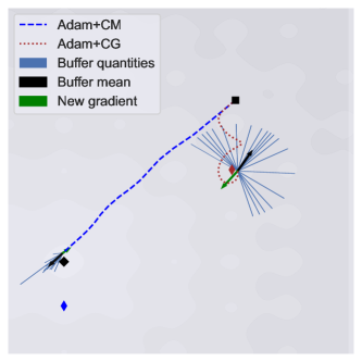
Figure 2: First $10$ steps of the Adam+CG and Adam+CM trajectories on Ackley loss surface. Coloured diamond represents the final points reached by the optimizers. Gradient cancellation is observed in Adam+CG on Ackley function as buffer mean and new gradients cancel each other out, which yields in a small update. On the other hand, Adam+CM escapes sub-optimal minima and converges near the global minimum.

The gradient cancellation problem.

However, as we observe throughout this paper, combining Adam with critical gradients does not always perform well. We hypothesize that in CG, while the buffer gradients can promote exploration initially (as observed in Figure 1), the parameters remain stuck in sharp regions due to gradient cancellation. Gradient cancellation primarily occurs when existing buffer gradients get quickly replaced by high-magnitude gradients when the parameters are near a sharp basin. As a result, the buffer quickly converges to high variance gradients whose mean goes to zero, allowing learning to converge. Intuitively, the parameters bounce back and forth off the sides and bottom of the sharp basin: whenever the parameters try to escape the basin, the new outgoing gradient gets cancelled by incoming gradients in the buffer. Figure 2 illustrates this phenomenon on a toy surface, by showing the buffer gradients (thin blue lines) and their means (black arrow) as well as the new gradient (green arrow), within sharp basins where Adam+CG gets stuck. Additional plots can be found in Appendix A.1.

Critical momenta (CM).

We have seen that gradient cancellation hinders the ability of Adam+CG to escape sharp minima. To fix this problem, our approach leverages instead a buffer $\textbf{m}_{c}$ of critical momenta $m_{c}$ during training. Just like in [35], we use the gradient $l_{2}$-norm, as priority criterion. The buffer takes the form of a dictionary where the key-value pairs are $(\|g_{c}\|_{2},m_{c})$ with a decay factor $\lambda\in(0,1)$ for the keys at each iteration. The integration with critical momenta leads to a new algorithm, Adam+CM, which defines the moment updates as follow:

$$m_{t} =\beta_{1}m_{t-1}+(1-\beta_{1})g_{t};~{}~{}~{}m^{M}_{t}=\texttt{aggr}(m_{t},\textbf{m}_{c})$$ (4)

$$v^{M}_{t} =\beta_{2}v^{M}_{t-1}+(1-\beta_{2})~{}\texttt{aggr}(m_{t},\textbf{m}_{c})^{2}$$ (5)

where aggr is the addition of the current momentum to the average of all critical momenta:

$$\texttt{aggr}(m_{t},\textbf{m}_{c})=m_{t}+\frac{1}{C}\sum_{m_{c}\in\textbf{m}_{c}}m_{c}\,.$$ (6)

Finally, the Adam+CM update rule is given by

$$\hat{m}^{M}_{t}=\frac{m^{M}_{t}}{1-\beta_{1}^{t}};~{}~{}~{}\hat{v}^{M}_{t}=\frac{v^{M}_{t}}{1-\beta_{2}^{t}};~{}~{}~{}\theta_{t+1}=\theta_{t}-\alpha\frac{\hat{m}^{M}_{t}}{\sqrt{\hat{v}^{M}_{t}+\epsilon}}$$ (7)

The pseudo-code of Adam+CM is given in Algorithm 1.

Looking at Figure 1, while at a sharp minima, the elements of the buffer will still be quickly replaced, due to the inertia in the momentum terms the variance will stay low. Moreover, the fact that gradients quickly change direction will lead to the new momentum terms being smaller and hence have a smaller immediate influence on the aggregate value of the buffer. This allows the overshooting effect to still happen, enabling the exploration effect and helping to learn to escape sharp minima. Furthermore, the larger the size of the buffer, the stronger the overshooting effect will be and the wider the minima needs to be for learning to converge. That is because learning needs to stay long enough in the basin of a minima to fill up most of the buffer in order to turn back to the minimum that it jumped over and for the optimizer to converge. We observe this empirically in Figure 8 and Appendix A.2.2.

4 Insights from toy examples

In this section, we empirically validate on toy tasks our working hypothesis by analyzing and comparing various combinations of Adam with memory augmentation and sharpness-aware minimization.

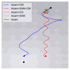
Figure 3: Training loss curves (left, averaged across $10$ seeds) and learning trajectories (right, one seed) for different optimizers on the Ackley loss surface. While the other optimizers get stuck in sub-optimal minima near the initialization point (black square), both CM variants explore and find the lower loss surface near the global solution (black diamond).

Critical momenta promote exploration.

We first compare the optimization trajectories of Adam+CM with Adam, Adam+SAM, and Adam+CG, on interpretable, non-convex $2$D loss surfaces. We also include the double combination of Adam with SAM and CM. To complement the Goldstein-Price function in Figure 1, we consider the Ackley function [1] (see (9) in Appendix A.2.1 for the explicit formula), which contains a nearly flat outer region with many sharp minima and a large hole at the center with the global minimum at $(0,0)$.

We minimize the Ackley function for $10$ different initialization seeds, and compare the trajectories of the different optimizers. We run each model for $500$ steps and reduce the learning rate by a factor $10$ at the $250$th step. To get the best performing setup, we perform a grid search over the hyper-parameters for each optimizer. Figure 3 shows the training curves (left) and optimization trajectories (right) of the different optimizers, for the same initialization (black square). We observe that, here, only the CM variants are able to explore the loss surface, resulting in a lower loss solution.

Additional trajectories with various different seeds for both the Ackley and Goldstein-Price loss surfaces are shown in Appendix A.2.1 (Figures 14 and 13).

Figure 4: Escape ratio (number of times the optimizer escapes the sharp minimum to reach the global minimum out of $50$ runs) in the $10$-D toy example (8), for different values of the sharpness coefficient. Adam+CM shows a higher ability to escape sharp minima in this setting.

	Optimizers	Loss	Sharpness
	Adam	$0.86$	$1.49$
	Adam+SAM	$3.14$	$1.43$
GP	Adam+CG	$0.85$	$1.51$
	Adam+CM	0.81	1.36
	Adam	$13.87$	$65.65$
	Adam+SAM	$13.87$	$65.62$
Levy	Adam+CG	$13.61$	$64.45$
	Adam+CM	12.50	62.53

Figure 5: Loss vs sharpness of the solutions of different optimizers for toy loss surfaces. The buffer decay is set to $0.99$ for these experiments. Adam+CM is able to find solutions that are both flatter and deeper (lower loss) than other optimizers in this setting.

Critical momenta reduce sharpness.

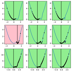
Figure 6: Optimization trajectory of Adam (left), Adam+CG (middle), and Adam+CM (right) on a toy 1D function with a flat and a sharp minimum with increasing sharpness (across columns), for different initialization points (across rows). Green backgrounds indicate that the optimizer escapes the sharper minimum while red backgrounds indicate otherwise. The vertical line indicates the final point in each sub-figure. We observe that Adam mostly converges to the minimum closest to the initial point. Adam+CM converges to the flatter minimum for different initial points and degrees of sharpness more often than Adam+CG.

We now want to compare more specifically the implicit bias of the different optimizers towards flat regions of the loss landscape.

We first examine the solutions of optimizers trained on the Goldstein-Price and Levy functions [29] (see Appendix A.2.1). Both of these functions contain several local minima and one global minimum. We evaluate the solutions based on the final loss and sharpness, averaged across $20$ seeds. As a simple proxy for sharpness, we compute the highest eigenvalue of the loss Hessian.

Results in Table 5 show that Adam+CM finds flatter solutions with a lower loss value compared to Adam, Adam+CG, and Adam+SAM in both examples. Furthermore, Adam and Adam+SAM reach almost equal loss values for the Levy function with a negligible difference in sharpness, but for the GP function, Adam+SAM converges to a sub-optimal minimum with lower sharpness.

We hypothesize that the buffer size controls the amount of exploration and analyze this empirically in Appendix A.2.1, where we show that even with a small buffer size, Adam+CM can escape sharper minima and explores lower loss regions than other optimizers. The results also suggest that in a controlled setting, the larger buffer size helps find a flatter minimum.

To further investigate the escaping abilities of the various optimizers, we consider the following class of functions on $\mathbb{R}^{D}$:

$$f_{s}(x)=\sum_{d=1}^{D}\text{min}(x_{d}^{2},s(x_{d}-1)^{2})$$ (8)

where $s>1$ is a sharpness coefficient. Each function in this class has two global minima: a flat minimum at the origin and a sharper minimum at $(1\cdots 1)$. Figure 6 shows optimization trajectories in the one-dimensional case for various values of the sharpness coefficient $s\in\{5,10,100\}$ (across columns) and initial point $x\in\{-2,2,3\}$ (across rows). We can see that Adam mostly converges to the minimum closest to the initial point. Adam+CM converges to the flatter minimum for different initial points and degrees of sharpness more often than Adam+CG. Additional plots are shown in Appendix A.3 for various values of the hyperparameters.

To quantify this bias in higher dimension ($D=10$), we sample $50$ different initial points uniformly in $[-5,5]^{10}$. Out of these $50$ runs, we count the number of times an optimizer finds the flat minimum at the origin by escaping the sharper minimum. Figure 5 reports the escape ratio for different values of the sharpness coefficient. We observe that Adam+CM (with buffer capacity $C=20$) has a higher escape ratio than others as the sharpness increases. We replicate this experiment with various values of the buffer capacity in Appendix A.2.1 (Figure 12).

5 Experimental results

The goal of this section is to evaluate our method empirically on complex models and benchmarks. All our results are averaged across three seeds.

5.1 Language modelling

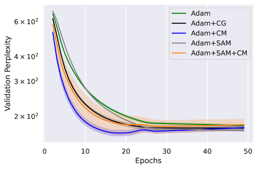
Figure 7: Validation perplexity of the different optimizers and Adam+CM using a single-layer LSTM trained on the PTB dataset. We see that Adam+CM and its SAM variant result in a lower validation perplexity and faster convergence.

Starting with a language-based task, a single-layer long short-term memory network (LSTM) [20] is trained on the Penn Tree Bank (PTB) dataset [34]. We evaluate the performance by reporting the validation perplexity on a held-out set. All models and optimizers are trained for $50$ epochs. We train the models for $40$ epochs (similar to [35]) and we reduce the learning at the $25^{th}$ epoch by dividing it by $10$. The results are reported after performing a grid search over corresponding hyper-parameters. The details of this grid search are present in Appendix Table 5.

Figure 7 shows the validation perplexity during the learning process. We observe that Adam+CM always converges faster, suggesting that it has explored and found a basin with a better generalizable solution than other optimizers by the $18$th epoch. The second-best performing optimizer is Adam+CG, which reaches lower perplexity after reducing the learning rate. Additionally, both CM variants overfit after convergence.

5.2 Image classification

Next, we evaluate the effect of Adam+CM on different model sizes for image classification.

CIFAR 10/100 [27]

We train ResNet models [17], particularly ResNet34 and WRN-1 (with 40 layers) [51]) for 3 different seeds. Optimizers are compared in terms of the validation accuracy computed on a held-out set. We train the models for 100 epochs where we reduce the learning at the $50$th epoch by dividing it by $10$.

Table 1: Comparison of performance in terms of best validation accuracy (%) achieved by the existing baselines with Adam+CM and its SAM variant on training ResNet34 and WRN-1 with CIFAR-10 and CIFAR-100. All measurements are averaged across 3 runs.

		CIFAR-10		CIFAR-100
Grid search	Optimizers	ResNet34	WRN-1	ResNet34	WRN-1
	Adam [26]	$93.6_{\pm 4.1}$	$90.5_{\pm 1.1}$	$69.6_{\pm 0.5}$	$61.9_{\pm 0.4}$
	Adam+CG [35]	$93.3_{\pm 1.6}$	$89.7_{\pm 1.4}$	$69.3_{\pm 0.2}$	$62.2_{\pm 1.0}$
✗	Adam+SAM [15]	$93.6_{\pm 4.4}$	$90.3_{\pm 3.5}$	$69.5_{\pm 0.1}$	$62.1_{\pm 0.3}$
	Adam+CM	$\textbf{93.7}_{\pm 2.4}$	$90.7_{\pm 2.4}$	$\textbf{69.8}_{\pm 1.4}$	$61.7_{\pm 0.3}$
	Adam+SAM+CM	$93.4_{\pm 5.3}$	$\textbf{91.0}_{\pm 1.3}$	$68.2_{\pm 0.1}$	$\textbf{63.1}_{\pm 0.2}$
	Adam [26]	$93.9_{\pm 0.3}$	$91.1_{\pm 0.6}$	$70.7_{\pm 0.3}$	$62.8_{\pm 0.3}$
	Adam+CG [35]	$93.8_{\pm 0.4}$	$90.6_{\pm 0.3}$	$71.0_{\pm 0.3}$	$63.4_{\pm 0.5}$
✓	Adam+SAM [15]	$93.7_{\pm 2.6}$	$90.5_{\pm 3.8}$	${70.5}_{\pm 0.4}$	$62.4_{\pm 0.5}$
	Adam+CM	${94.0}_{\pm 0.3}$	${91.5}_{\pm 0.1}$	${\textbf{71.2}}_{\pm 0.3}$	${\textbf{63.6}}_{\pm 0.6}$
	Adam+SAM+CM	${\textbf{94.5}}_{\pm 2.3}$	${\textbf{91.7}}_{\pm 2.0}$	$69.7_{\pm 0.3}$	${63.1}_{\pm 0.5}$

Results from all experiments performed for image classification tasks are summarized in Table 1, where we report the best validation accuracy achieved by different ResNet models when they are trained on CIFAR-10/100. We report the results both with and without performing an extensive grid search over hyper-parameters. The details of this grid search are present in Appendix Table 5.

In each case, we observe that CM variants perform best. Without grid search, CM variants perform best on both datasets, with Adam+CM achieving the best results with the ResNet34 model while Adam+SAM+CM performs best with the WRN-1 model. With grid search, Adam+SAM+CM yielded the best validation accuracy for CIFAR-10, while Adam+CM performed the best on CIFAR-100.

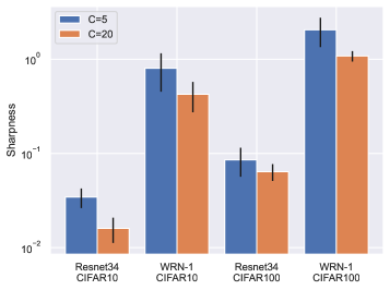
Figure 8: (Left) Validation accuracy with default hyper-parameterson CIFAR-10 for WRN-1. In this case, Adam+SAM+CM results in the best performance. (Right) Sharpness for different buffer sizes for Adam+CM CIFAR10/100 experiments with the same hyper-parameter setup. Using a larger buffer size results in lower sharpness even for high-dimensional models.

Figure 8 (left) shows the training progress of the different optimizers without grid search, where we see CM variants have slightly faster convergence in WRN-1 and Adam+SAM+CM outperform other baselines when the learning rate is reduced after the $50$th epoch. Similar plots with and without grid search are given in Appendix A.2.2. Figure 8 (right) shows the final sharpness metric for different buffer sizes recorded for CIFAR10/100 experiments with default hyperparameter setup. It is clear that using a large buffer size can further reduce the sharpness of the solution in such complex settings.

ImageNet [8]

We also train an EfficientNet-B0 model [46] from scratch on ImageNet. We used a publicly available EfficientNet implementation in PyTorch [39], weight decay [33] of $1$e-$4$ and an initial learning rate of $1$e-$4$ which is reduced by a factor of $10$ every $30$ epochs. We provide additional details about the datasets and models in Appendix A.2.

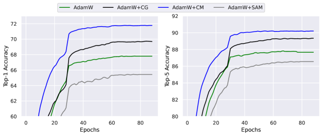
Figure 9: Top-1 accuracy (left), top-5 accuracy (right) of the different optimizers and AdamW+CM training an EfficientNet-B0 on ImageNet. All optimizers use the same weight decay and learning rate scheduler. AdamW+CM outperform existing optimizers with default settings.

Figure 9 compares top-1 and top-5 accuracies on the validation set. Due to compute constraints, we use the default hyper-parameter set. We observe that AdamW+CM convergences faster and achieves better final top-1 and top-5 accuracies than the other optimizer baselines whereas SAM does not perform well in the default hyper-parameter setting.

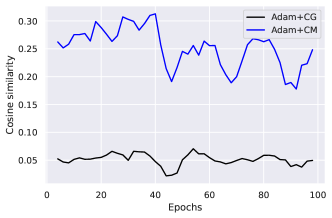
Figure 10: Sharpness (top-left), distance (top-right) buffer variance (bottom-left) and cosine similarity (bottom-right) in buffer elements of the optimizers using WRN-1 on CIFAR-100. These indicate that buffer elements in Adam+CM agree more with each other and have lower sharpness than Adam+CG.

5.2.1 Analysis

Figure 10 corroborates the claim in Section 4 that Adam+CM finds a flatter surface containing the global minimum, as the top-right plot shows lower sharpness when compared to Adam or Adam+SAM. It also reveals the greater distance travelled by parameters during training, which indicates that using CM promotes more exploration than the other optimizers.

The bottom-left plot in Figure 10 shows that buffer elements stored by Adam+CM have lower variance during training compared to Adam+CG. To compare the agreement among buffer quantities, we take the element with the highest norm within the buffer, compute the cosine similarities with other elements in the buffer, and take the mean of these similarities. The bottom-right plot in Figure 10 shows that the agreement in Adam+CM remains higher than in Adam+CG, indicating that the aggregation of buffer elements in Adam+CM will more often result in a non-zero quantity in the desired direction. On the other hand, high variance and disagreement among elements in the Adam+CG buffer may cause gradient cancellation during aggregation and result in Adam-like behavior.

6 Conclusion

This work introduces a framework for promoting exploration in adaptive optimizers. We propose Adam+CM, a new memory-augmented version of Adam that maintains a buffer of critical momenta and modifies the parameters update rule using an aggregation function. Our analysis shows that it addresses the drawbacks of existing memory-augmented adaptive optimizers and promotes exploration towards flatter regions of the loss landscape. Our empirical results show that Adam+CM outperforms Adam, SAM, and CG on standard image classification and language modeling tasks. For large-scale models, CM provides exploration benefits by searching for flat loss surfaces.

A promising avenue of investigation is to apply our method to non-stationary settings like continual learning, as these require the model to transfer knowledge without overfitting on a single task. Our results suggest that CM may be able to capture higher-order dynamics of the loss surface, deserving further exploration. We leave the theoretical in-depth analysis for future work.

Appendix A Appendix

In this section, we provide the details and results not present in the main content. In section A.1, we report more evidence of gradient cancellation in a toy example. In section A.2, we describe the implementation details including hyper-parameters values used in our experiments. All experiments were executed on an NVIDIA A100 Tensor Core GPUs machine with 40 GB memory.

A.1 Gradient cancellation in CG

When we track the trajectory along with the gradient directions of the buffer in the Adam+CG optimizer on the Ackley+Rosenbrock function (defined in the next section), we found that CG gets stuck in the sharp minima (see Figure 11). This is because of the gradient cancellation problem discussed earlier.

Figure 11: Three consecutive steps in training Adam+CG on Ackley+Rosenbrock function with $C=5$. The white lines indicate the gradient directions in the buffer. Since four of these gradients point in opposite directions, their mean would be small and cancel the current gradient update out. As a result, parameters get stuck in the sharp minima.

A.2 Implementation details and other results

A.2.1 Toy examples

We evaluate our optimizer on the following test functions in Section 4:

1. Ackley function:

   $$f(x,y)=-20\exp(-0.2\sqrt{0.5(x^{2}+y^{2})})-\exp(0.5(\cos{2\pi x}+\cos{2\pi y}))+e+20$$ (9)

   The global minimum is present at $(0,0)$. In Figure 13, we visualize the trajectories of Adam, Adam+SAM, Adam+CG and Adam+CM for different initialization points. While other optimizers may get stuck at nearby local minima, Adam+CM benefits from more exploration and finds a lower-loss surface that may contain the global minima.

2. Goldstein-Price function:

   $$f(x,y) =\frac{1}{2.427}\log[1+(x+y+1)^{2}(19-14x+3x^{2}-14y+6xy+3y^{2})]$$ (10)

   $$\times[30+(2x-3y)^{2}(18-32x+12x^{2}+48y-36xy+27y^{2})-8.693]$$

   The global minimum is present at $[0,1]^{2}$. In Figure 14, we visualize the trajectories of Adam, Adam+SAM, Adam+CG and Adam+CM for different initialization points. While other optimizers may get stuck at a sub-optimal loss surface, Adam+CM benefits from more exploration and finds the global minimum.

3. Levy function:

   $$f(x_{1},x_{2})=\sin^{2}(\pi w)+\sum_{i=1}^{d-1}(w_{i}-1)^{2}[1+10\sin^{2}(\pi w_{i}+1)]+(w_{d}-1)^{2}[1+\sin^{2}(2\pi w_{d})]$$ (11)

   where $w_{i}=1+\frac{x_{i}-1}{4}$ and $d$ is the number of variables. The global minimum is present at $(1,1)$.

4. Ackley+Rosenbrock function:

   $$f(x,y)=0.05(1-x)^{2}+0.05(y-x^{2})^{2}+0.6[\exp(-0.2\sqrt{0.5(x^{2}+y^{2})})$$ (12)

   $$-\exp(0.5(\cos{2\pi x}+\cos{2\pi y}))+e]$$

   The global minima is present at $(2.1,3.9)$.

In Figure 12 (left), we compare the escape ratio for different optimizers on Equation 8 with $d=1$ (similar to Figure 5). We can see that for $\texttt{C}=10$, with an exception at $s=2$, Adam+CM consistently finds the minimum at $x=0$ more often than other optimizers. Interestingly, as $s$ increases, Adam+CG is outperformed by both Adam and Adam+SAM, which indicates that Adam+CG is more susceptible to getting stuck at sharper minima in this example. Figure 12 (right) shows that the tendency of Adam+CM to escape minima is dependent on C such that, a larger value of C results in convergence to flatter minimum more often.

Figure 12: (i) Escape ratio (number of times when optimizer reaches the minima at $x=0$ out of total $50$ runs) for different sharpness coefficient ($s$) for minima at $x=1$ in 1D toy example shown in Figure 6. (ii) Escape ratio vs sharpness coefficient ($s$) for different $C$.

In Table 5, we also compared different optimizers in terms of the sharpness of the solution reached by each optimizer on different functions. In Table 2, we perform a similar experiment and compare sharpness across different values of hyperparameters for Adam+CM. We observe that Adam+CM is able to find a flatter and lower-loss solution as buffer size increases. This is consistent with complex tasks in Figure 8.

Table 2: Loss vs sharpness of the solutions of Adam+CM for different hyperparameters buffer sizes on Levy function. Adam+CM is able to find solutions that are both flatter and deeper (lower loss) as buffer size increases. Moreover, Adam+CM always outperforms Adam+CG even with a smaller buffer size.

Optimizers	C	$\lambda$	Loss	Sharpness
Adam+CG	$5$	$0.7$	${14.40}$	${64.72}$
Adam+CG	$5$	$0.99$	${14.41}$	${64.67}$
Adam+CG	$20$	$0.99$	$13.61$	$64.45$
Adam+CM	$5$	$0.7$	${12.90}$	${63.74}$
Adam+CM	$5$	$0.99$	${13.02}$	${63.83}$
Adam+CM	$20$	$0.99$	12.50	62.53

Figure 13: Optimization trajectories of various optimizers on the Ackley loss surface for different initial points (black square). The black diamond indicates the global minimum.

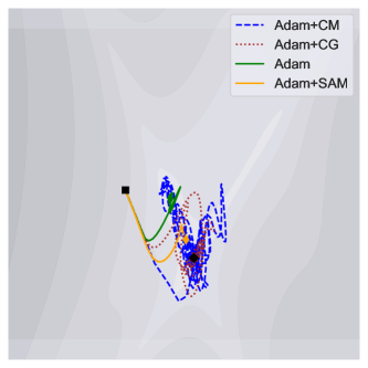
Figure 14: Optimization trajectories of various optimizers on the Goldstein-Price loss surface for different initial points (black square). The black diamond indicates the global minimum..

A.2.2 Deep learning experiments

In Table 3 and Table 4, we provide a summary of all datasets and deep learning models used in the experiment from Section 5.

Table 3: Dataset details

Dataset	Train set	Validation set
PTB	890K	70K
CIFAR-10	40K	10K
CIFAR-100	40K	10K
ImageNet	1281K	50K

The tasks consist of:

• The Penn Treebank (PTB) is a part-of-speech (POS) tagging task where a model must determine what part of speech (ex. verb, subject, direct object, etc.) every element of a given natural language sentence consists of.

• CIFAR-10 is a multiclass image classification task the training and validation set consists of images that are separated into 10 distinct classes, with each class containing an equal number of samples across the training and validation sets. The goal is to predict the correct image class, provided as an annotated label, given a sample from the sets.

• CIFAR-100 is the same task as CIFAR-10, except that images are now separated into 100 classes with an equal number of samples within each class.

• ImageNet is a large-scale dataset consisting of images separated into 1000 distinct classes. The objective of the task is the same as CIFAR-10 and CIFAR-100, which is to classify images from the training and validation set correctly into a class with an annotated label.

Table 4: Model details

Model	Number of parameters
LSTM	20K
WRN-2	11M
WRN-2	45M
ResNet34	22M
WRN-1	0.5M
EfficientNet-B0	5.3M

For all toy examples experiments based on Equation 8, the learning rate is set as $0.05$. The learning rate is set as $0.1$ for other toy examples. For the results reported in Table 1, we run a grid search only over the learning rate for CIFAR10/100 experiments that work best for a given model using Adam and keep that learning rate fixed for all other optimizers for comparison. For all Imagenet experiments, the learning rate is set to $0.0001$. Unless specified in the experiment description, the default set of other hyperparameters in all our experiments is $\{\beta_{1},\beta_{2},\texttt{C},\lambda,\rho\}=\{0.9,0.99,5,0.7,0.05\}$ except in CIFAR10/100 experiments where $\beta_{2}$ is set to $0.999$. The default values of C and $\lambda$ are decided based on the suggested values from [35] and $\rho$ based on [15]. For the results in Figure 5 and Table 5, C and $\lambda$ are est to $20$ and $0.99$.

For PTB and CIFAR10/100, we provide the details on hyper-parameter grid-search in Table 5 and the best settings for all experiments and Table 6, Table 7 and Table 8. In these tables, we report the hyperparameter set for each optimizer as follows:

• Adam: $\{\alpha\}$

• Adam+CG: $\{\alpha,\beta_{1},\beta_{2},\texttt{C},\lambda\}$

• Adam+SAM: $\{\alpha,\beta_{1},\beta_{2},\rho\}$

• Adam+CM: $\{\alpha,\beta_{1},\beta_{2},\texttt{C},\lambda\}$

• Adam+SAM+CM: $\{\alpha,\beta_{1},\beta_{2},\texttt{C},\lambda,\rho\}$

Table 5: Details on grid search on hyper-parameter setting.

Hyper-parameter	Set
lr	$\{0.1,0.01,0.001,0.0001\}$
$\beta_{1}$	$\{0.9,0.99,0.999\}$
$\beta_{2}$	$\{0.99,0.999,0.9999\}$
C	$\{5,20\}$
$\lambda$	$\{0.7,0.99\}$
$\rho$	$\{0.01,0.05,0.1\}$

Table 6: Best hyperparameter settings for different optimizers on PTB.

Optimizers	PTB
	LSTM
Adam	{0.001, 0.9, 0.99}
Adam+CG	{0.001, 0.9, 0.999, 5, 0.7}
Adam+SAM	{0.001, 0.9, 0.9, 0.01}
Adam+CM	{0.001, 0.9, 0.999, 5, 0.7}
Adam+SAM+CM	{0.001, 0.9, 0.999, 5, 0.7, 0.1}

Table 7: Best hyperparameter settings for different optimizers on CIFAR10.

	CIFAR10
Optimizers	Resnet34	WRN1
Adam	{0.001, 0.9, 0.999}	{0.01, 0.9, 0.999}
Adam+CG	{0.0001, 0.9, 0.999, 20, 0.7}	{0.001, 0.9, 0.99, 20, 0.7}
Adam+SAM	{0.0001, 0.9, 0.99, 0.05}	{0.01, 0.9, 0.9999, 0.1}
Adam+CM	{0.0001, 0.9, 0.999, 20, 0.99}	{0.001, 0.9, 0.999, 5, 0.7}
Adam+SAM+CM	{0.0001, 0.9, 0.99, 20, 0.99, 0.05}	{0.001, 0.9, 0.9999, 20, 0.7, 0.1}

Table 8: Best hyperparameter settings for different optimizers on CIFAR100.

	CIFAR100
Optimizers	Resnet34	WRN1
Adam	{0.0001, 0.9, 0.9999}	{0.001, 0.9, 0.99}
Adam+CG	{0.0001, 0.9, 0.9999, 20, 0.7}	{0.001, 0.9, 0.99, 20, 0.7}
Adam+SAM	{0.0001, 0.9, 0.999, 0.1}	{0.001, 0.9, 0.999, 0.05}
Adam+CM	{0.0001, 0.9, 0.999, 20, 0.99}	{0.001, 0.9, 0.9999, 5, 0.7}
Adam+SAM+CM	{0.0001, 0.9, 0.9999, 20, 0.7, 0.05}	{0.001, 0.9, 0.99, 5, 0.7, 0.1}

Next, similar to Figure 8, we plot the training process in CIFAR-10/100 on ResNet34 and WRN-1 models with hyperparameter tuning (see Figure 15) and without hyper-parameter tuning (see Figure 16). Overall, we can see that while Adma+SAM can have faster convergence, the CM variants reach higher validation accuracy in both setups.

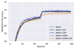
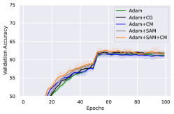
Figure 15: Validation accuracy of the different optimizers and Adam+CM with default hyper-parameterson CIFAR-10 for ResNet34 (left) and CIFAR-100 for ResNet34 (middle) and WRN-1 (right). Overall, Adam+SAM+CM results in the best performance.

Figure 16: Validation accuracy of the different optimizers and Adam+CM with hyper-parameter search on CIFAR-10 (left column) and CIFAR-100 (right column) for ResNet34 (first row) and WRN-1 (second row).

A.3 Sensitivity analysis on toy example

Following experiments in Figure 6 in section 4, we fix decay to $0.7$ in Figure 17 and vary C. We perform a similar experiment with decay$=0.99$ and plot them in Figure 18. In both these figures, the observation remains the same that is Adam+CM converges to flatter minima for different initial points and degrees of sharpness. We also observe that C plays an important role in convergence to flatter minima in both Adam+CG and Adam+CM.

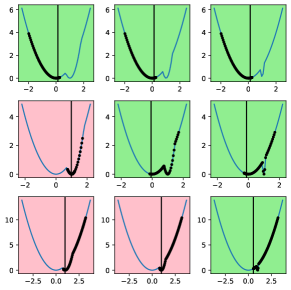
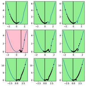
Figure 17: Following Figure 6, we compare trajectories of Adam+CG (left columns) and Adam+CM (right column) on Equation 8 with $d=1$ where $\lambda$ is set to $0.7$ and C: (i) $5$ (first row), (ii) $10$ (second row) and (iii) $20$ (third row). For different initial points and degrees of sharpness, Adam+CM converges to flatter minima more often than Adam+CG.

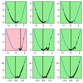
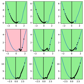
Figure 18: Following Figure 6, we compare trajectories of Adam+CG (left columns) and Adam+CM (right column) on Equation 8 with $d=1$ where $\lambda set$ to $0.99$ and C: (i) $5$ (first row), (ii) $10$ (second row) and (iii) $20$ (third row). For different initial points and degrees of sharpness, Adam+CM converges to flatter minima more often than Adam+CG.

References

- Ackley [1987] David H Ackley. The model. In A Connectionist Machine for Genetic Hillclimbing, pages 29–70. Springer, 1987.
- Chaudhari et al. [2017] Pratik Chaudhari, Anna Choromanska, Stefano Soatto, Yann LeCun, Carlo Baldassi, Christian Borgs, Jennifer Chayes, Levent Sagun, and Riccardo Zecchina. Entropy-SGD: Biasing gradient descent into wide valleys. In International Conference on Learning Representations, 2017.
- Chen et al. [2022] Xiangning Chen, Cho-Jui Hsieh, and Boqing Gong. When vision transformers outperform resnets without pre-training or strong data augmentations. In International Conference on Learning Representations, 2022.
- Choi et al. [2019] Dami Choi, Christopher J Shallue, Zachary Nado, Jaehoon Lee, Chris J Maddison, and George E Dahl. On empirical comparisons of optimizers for deep learning. arXiv preprint arXiv:1910.05446, 2019.
- Cohen et al. [2022] Jeremy M Cohen, Behrooz Ghorbani, Shankar Krishnan, Naman Agarwal, Sourabh Medapati, Michal Badura, Daniel Suo, David Cardoze, Zachary Nado, George E Dahl, et al. Adaptive gradient methods at the edge of stability. arXiv preprint arXiv:2207.14484, 2022.
- Defazio and Jelassi [2022] Aaron Defazio and Samy Jelassi. Adaptivity without compromise: a momentumized, adaptive, dual averaged gradient method for stochastic optimization. Journal of Machine Learning Research, 2022.
- Defazio et al. [2014] Aaron Defazio, Francis Bach, and Simon Lacoste-Julien. SAGA: A fast incremental gradient method with support for non-strongly convex composite objectives. Advances in Neural Information Processing Systems, 2014.
- Deng et al. [2009] Jia Deng, Wei Dong, Richard Socher, Li-Jia Li, Kai Li, and Li Fei-Fei. ImageNet: A large-scale hierarchical image database. In IEEE Conference on Computer Vision and Pattern Recognition, 2009.
- Dosovitskiy et al. [2021] Alexey Dosovitskiy, Lucas Beyer, Alexander Kolesnikov, Dirk Weissenborn, Xiaohua Zhai, Thomas Unterthiner, Mostafa Dehghani, Matthias Minderer, Georg Heigold, Sylvain Gelly, Jakob Uszkoreit, and Neil Houlsby. An image is worth 16x16 words: Transformers for image recognition at scale. In International Conference on Learning Representations, 2021.
- Dozat [2016] Timothy Dozat. Incorporating Nesterov momentum into Adam. In International Conference on Learning Representations workshop, 2016.
- Du et al. [2022a] Jiawei Du, Zhou Daquan, Jiashi Feng, Vincent Tan, and Joey Tianyi Zhou. Sharpness-aware training for free. In Advances in Neural Information Processing Systems, 2022a.
- Du et al. [2022b] Jiawei Du, Hanshu Yan, Jiashi Feng, Joey Tianyi Zhou, Liangli Zhen, Rick Siow Mong Goh, and Vincent Tan. Efficient sharpness-aware minimization for improved training of neural networks. In International Conference on Learning Representations, 2022b.
- Duchi et al. [2011] John Duchi, Elad Hazan, and Yoram Singer. Adaptive subgradient methods for online learning and stochastic optimization. Journal of Machine Learning Research, 2011.
- Dziugaite and Roy [2017] Gintare Karolina Dziugaite and Daniel M. Roy. Computing nonvacuous generalization bounds for deep (stochastic) neural networks with many more parameters than training data. In Conference on Uncertainty in Artificial Intelligence, 2017.
- Foret et al. [2021] Pierre Foret, Ariel Kleiner, Hossein Mobahi, and Behnam Neyshabur. Sharpness-aware minimization for efficiently improving generalization. In International Conference on Learning Representations, 2021.
- Granziol et al. [2020] Diego Granziol, Xingchen Wan, Samuel Albanie, and Stephen Roberts. Iterative averaging in the quest for best test error. arXiv preprint arXiv:2003.01247, 2020.
- He et al. [2016] Kaiming He, Xiangyu Zhang, Shaoqing Ren, and Jian Sun. Deep residual learning for image recognition. In IEEE Conference on Computer Vision and Pattern Recognition, 2016.
- Hinton et al. [2012] Geoffrey Hinton, Nitish Srivastava, and Kevin Swersky. Neural networks for machine learning lecture 6a overview of mini-batch gradient descent, 2012.
- Hochreiter and Schmidhuber [1994] Sepp Hochreiter and Jürgen Schmidhuber. Simplifying neural nets by discovering flat minima. Advances in Neural Information Processing Systems, 1994.
- Hochreiter and Schmidhuber [1997] Sepp Hochreiter and Jürgen Schmidhuber. Long short-term memory. Neural Computation, 9:1735–1780, 1997.
- Izmailov et al. [2018] Pavel Izmailov, Dmitrii Podoprikhin, Timur Garipov, Dmitry P. Vetrov, and Andrew Gordon Wilson. Averaging weights leads to wider optima and better generalization. In Conference on Uncertainty in Artificial Intelligence, 2018.
- Jiang* et al. [2020] Yiding Jiang*, Behnam Neyshabur*, Hossein Mobahi, Dilip Krishnan, and Samy Bengio. Fantastic generalization measures and where to find them. In International Conference on Learning Representations, 2020.
- Kaur et al. [2022] Simran Kaur, Jeremy Cohen, and Zachary C Lipton. On the maximum hessian eigenvalue and generalization. arXiv preprint arXiv:2206.10654, 2022.
- Keskar et al. [2016] Nitish Shirish Keskar, Dheevatsa Mudigere, Jorge Nocedal, Mikhail Smelyanskiy, and Ping Tak Peter Tang. On large-batch training for deep learning: Generalization gap and sharp minima. In International Conference on Learning Representations, 2016.
- Kim et al. [2022] Minyoung Kim, Da Li, Shell X Hu, and Timothy Hospedales. Fisher SAM: Information geometry and sharpness aware minimisation. In International Conference on Machine Learning, 2022.
- Kingma and Ba [2015] Diederik P Kingma and Jimmy Ba. Adam: A method for stochastic optimization. In International Conference on Learning Representations, 2015.
- Krizhevsky et al. [2009] Alex Krizhevsky, Geoffrey Hinton, et al. Learning multiple layers of features from tiny images, 2009.
- Kwon et al. [2021] Jungmin Kwon, Jeongseop Kim, Hyunseo Park, and In Kwon Choi. ASAM: Adaptive sharpness-aware minimization for scale-invariant learning of deep neural networks. In International Conference on Machine Learning, 2021.
- Laguna and Marti [2005] Manuel Laguna and Rafael Marti. Experimental testing of advanced scatter search designs for global optimization of multimodal functions. Journal of Global Optimization, 33:235–255, 2005.
- Le et al. [2011] Quoc V Le, Jiquan Ngiam, Adam Coates, Abhik Lahiri, Bobby Prochnow, and Andrew Y Ng. On optimization methods for deep learning. In International Conference on Machine Learning, 2011.
- Liu et al. [2023] Ren Liu, Fengmiao Bian, and Xiaoqun Zhang. Binary quantized network training with sharpness-aware minimization. Journal of Scientific Computing, 2023.
- Liu et al. [2022] Yong Liu, Siqi Mai, Xiangning Chen, Cho-Jui Hsieh, and Yang You. Towards efficient and scalable sharpness-aware minimization. In IEEE/CVF Conference on Computer Vision and Pattern Recognition, 2022.
- Loshchilov and Hutter [2019] Ilya Loshchilov and Frank Hutter. Decoupled weight decay regularization. In International Conference on Learning Representations, 2019.
- Marcus et al. [1993] Mitchell P. Marcus, Mary Ann Marcinkiewicz, and Beatrice Santorini. Building a large annotated corpus of english: The penn treebank. Comput. Linguist., 19(2):313–330, jun 1993. ISSN 0891-2017.
- McRae et al. [2022] Paul-Aymeric Martin McRae, Prasanna Parthasarathi, Mido Assran, and Sarath Chandar. Memory augmented optimizers for deep learning. In International Conference on Learning Representations, 2022.
- Mordido et al. [2022] Gonçalo Mordido, Sarath Chandar, and François Leduc-Primeau. Sharpness-aware training for accurate inference on noisy DNN accelerators. arXiv preprint arXiv:2211.11561, 2022.
- Neyshabur et al. [2017] Behnam Neyshabur, Srinadh Bhojanapalli, David McAllester, and Nati Srebro. Exploring generalization in deep learning. Advances in Neural Information Processing Systems, 2017.
- Nocedal [1980] Jorge Nocedal. Updating quasi-Newton matrices with limited storage. Mathematics of computation, 1980.
- Paszke et al. [2019] Adam Paszke, Sam Gross, Francisco Massa, Adam Lerer, James Bradbury, Gregory Chanan, Trevor Killeen, Zeming Lin, Natalia Gimelshein, Luca Antiga, et al. PyTorch: An imperative style, high-performance deep learning library. Advances in Neural Information Processing Systems, 2019.
- Picheny et al. [2013] Victor Picheny, Tobias Wagner, and David Ginsbourger. A benchmark of kriging-based infill criteria for noisy optimization. Structural and multidisciplinary optimization, 48:607–626, 2013.
- Polyak [1964] Boris T Polyak. Some methods of speeding up the convergence of iteration methods. USSR Computational Mathematics and Mathematical Physics, 1964.
- Robbins and Monro [1951] Herbert Robbins and Sutton Monro. A stochastic approximation method. The Annals of Mathematical Statistics, 1951.
- Roux et al. [2012] Nicolas Roux, Mark Schmidt, and Francis Bach. A stochastic gradient method with an exponential convergence rate for finite training sets. Advances in Neural Information Processing Systems, 2012.
- Schraudolph et al. [2007] Nicol N Schraudolph, Jin Yu, and Simon Günter. A stochastic quasi-newton method for online convex optimization. In Conference on Artificial Intelligence and Statistics, 2007.
- Shalev-Shwartz and Zhang [2013] Shai Shalev-Shwartz and Tong Zhang. Stochastic dual coordinate ascent methods for regularized loss minimization. Journal of Machine Learning Research, 2013.
- Tan and Le [2019] Mingxing Tan and Quoc Le. EfficientNet: Rethinking model scaling for convolutional neural networks. In International Conference on Machine Learning, 2019.
- Vaswani et al. [2017] Ashish Vaswani, Noam Shazeer, Niki Parmar, Jakob Uszkoreit, Llion Jones, Aidan N Gomez, Ł ukasz Kaiser, and Illia Polosukhin. Attention is all you need. In Advances in Neural Information Processing Systems, 2017.
- Wilson et al. [2017] Ashia C Wilson, Rebecca Roelofs, Mitchell Stern, Nati Srebro, and Benjamin Recht. The marginal value of adaptive gradient methods in machine learning. In Advances in Neural Information Processing Systems, 2017.
- Wu et al. [2018a] Lei Wu, Chao Ma, and Weinan E. How SGD selects the global minima in over-parameterized learning: A dynamical stability perspective. In Advances in Neural Information Processing Systems, 2018a.
- Wu et al. [2018b] Lei Wu, Chao Ma, et al. How SGD selects the global minima in over-parameterized learning: A dynamical stability perspective. Advances in Neural Information Processing Systems, 31, 2018b.
- Zagoruyko and Komodakis [2016] Sergey Zagoruyko and Nikos Komodakis. Wide residual networks. arXiv preprint arXiv:1605.07146, 2016.
- Zeiler [2012] Matthew D Zeiler. ADADELTA: An adaptive learning rate method. arXiv preprint arXiv:1212.5701, 2012.
- Zhou et al. [2020] Pan Zhou, Jiashi Feng, Chao Ma, Caiming Xiong, Steven Chu Hong Hoi, et al. Towards theoretically understanding why SGD generalizes better than Adam in deep learning. Advances in Neural Information Processing Systems, 2020.
- Zhuang et al. [2020] Juntang Zhuang, Tommy Tang, Yifan Ding, Sekhar C Tatikonda, Nicha Dvornek, Xenophon Papademetris, and James Duncan. AdaBelief optimizer: Adapting stepsizes by the belief in observed gradients. In Advances in Neural Information Processing Systems, 2020.
- Zhuang et al. [2022] Juntang Zhuang, Boqing Gong, Liangzhe Yuan, Yin Cui, Hartwig Adam, Nicha C Dvornek, Sekhar Tatikonda, James Duncan, and Ting Liu. Surrogate gap minimization improves sharpness-aware training. In International Conference on Learning Representations, 2022.
- Zou et al. [2021] Difan Zou, Yuan Cao, Yuanzhi Li, and Quanquan Gu. Understanding the generalization of Adam in learning neural networks with proper regularization. arXiv preprint arXiv:2108.11371, 2021.