Guided Linear Upsampling

Abstract.

Guided upsampling is an effective approach for accelerating high-resolution image processing. In this paper, we propose a simple yet effective guided upsampling method. Each pixel in the high-resolution image is represented as a linear interpolation of two low-resolution pixels, whose indices and weights are optimized to minimize the upsampling error. The downsampling can be jointly optimized in order to prevent missing small isolated regions. Our method can be derived from the color line model and local color transformations. Compared to previous methods, our method can better preserve detail effects while suppressing artifacts such as bleeding and blurring. It is efficient, easy to implement, and free of sensitive parameters. We evaluate the proposed method with a wide range of image operators, and show its advantages through quantitative and qualitative analysis. We demonstrate the advantages of our method for both interactive image editing and real-time high-resolution video processing. In particular, for interactive editing, the joint optimization can be precomputed, thus allowing for instant feedback without hardware acceleration.

Figure 1. Our method to accelerate high-resolution image processing with guided linear upsampling. Given a high-resolution source image $I$, our method can jointly optimize the downsampled source image $I^{{}_{\downarrow}}$ and the interpolation parameters $\Theta$, and then $I^{{}_{\downarrow}}$ is processed by a black-box image operator to get the low-resolution target image $T^{{}_{\downarrow}}$. The high-resolution target image $\hat{T}$ can be linearly upsampled from $T^{{}_{\downarrow}}$ with the optimized parameters $\Theta$.

1. Introduction

In the past decades, many useful image processing methods have been proposed for various tasks such as enhancement (Aubry et al., 2014), style transfer (Zhu et al., 2017; Li et al., 2018), matting (Levin et al., 2007), colorization (Iizuka et al., 2016), etc. Most of them require intensive computation and memory, and thus face great challenges for high-resolution images. At the same time, the popularity of mobile devices requires us to consider more about computational efficiency. The problem is even more prominent for interactive image editing (Levin et al., 2004; Bousseau et al., 2009), which requires repetitive user interactions, so instant feedback is necessary for a better user experience.

For general image processing, the guided upsampling should be the simplest and most effective way to achieve acceleration. By using the original image as a guidance map, a large ratio downsampling of the output image can be upsampled to the original resolution without noticeable artifacts. This is amazing because even for image operators of linear complexity in image size, using $8\times$ downsampling can result in $64\times$ speed up.

Two classical approaches for guided upsampling are joint bilateral upsampling (JBU) (Kopf et al., 2007) and bilateral guided upsampling (BGU) (Chen et al., 2016). JBU is an extension of the bilateral filter (Paris and Durand, 2006; Durand and Dorsey, 2002), while BGU is based on the local color transformations (Levin et al., 2007), whose effectiveness for guided upsampling has been demonstrated in earlier works such as transform recipes (Gharbi et al., 2015) and guided filter (He et al., 2012). In BGU, the local transformations are applied in the bilateral space (Barron et al., 2015), which further improves the efficiency and quality. Recent works are mainly learning-based (Gharbi et al., 2017; Xia et al., 2020, 2021; Dai et al., 2021), which can better employ domain knowledge for improving quality. However, they need to be trained for each specific task, and thus cannot be generalized to other tasks. Instead, we will follow the roadmap of the classical approaches, in order to seek a universal guided upsampler applicable to a wide range of image operators.

In this paper, we propose Guided Linear Upsampling (GLU), which is pretty simple but very effective. We introduce a new representation of high-resolution images, with each pixel represented as the linear interpolation of only two low-resolution pixels. By optimizing the representation parameters, i.e. the indices and weights of the interpolated pixel pairs, very small errors can be achieved even for large ratio upsampling. The parameters can be optimized for the source image and then applied to the target image, resulting in a high-resolution target image that can well preserve details while avoiding artifacts such as bleeding and blurring. We also propose an efficient method to optimize the downscaled source image, in order to better preserve thin structures and small regions. As illustrated in Figure 1, with our method the downsampling and upsampling can be jointly optimized in order to minimize the upsampling error, thus effectively preventing the loss of small isolated local structures.

The proposed method contains only a few parameters that are easy to set, and a fixed parameter setting can be well suited for various tasks and input images. It is efficient and easy to implement, and can achieve fast speed with a GPU implementation. Moreover, the joint optimization of upsampling and downsampling is target-free, i.e. independent of the target image, and thus needs to be done only once for each image, regardless of how the target image changes. As a demonstration, we show that with our method, real-time image editing and video processing can be achieved easily for time-costly image operators.

2. Related Work

The computational efficiency of image processing algorithms is very important for many applications, so it has attracted a lot of studies for various image processing tasks, such as filtering (Vaudrey and Klette, 2009; Liu and Shen, 2011), enhancement (Farbman et al., 2008) and modern learning-based image synthesis (Chai et al., 2022) etc. GPU-based acceleration has also been widely studied (Wu and Xu, 2009; Kazhdan and Hoppe, 2008; Li et al., 2012). Most of these methods are specific to the processing algorithms. In contrast, we will focus on guided upsampling, which can accelerate a wide range of image operators by treating them as black boxes.

The problem of guided upsampling is first introduced in (Kopf et al., 2007), in which joint bilateral upsampling (JBU) is proposed as the solution. JBU represents each output pixel as the weighted average of a set of low-resolution pixels. The weights are computed with bilateral weighting function (Tomasi and Manduchi, 1998) incorporating the guidance of the high-resolution input image. As a result, JBU also inherits the problems of the bilateral filter, such as edge blur and gradient reversal (Durand and Dorsey, 2002; He et al., 2012). Our method has the same general form as JBU, but it involves the weighted average of only two pixels, and the artifacts can be avoided by the proposed optimization techniques.

In guided image filtering (He et al., 2012), the target image is locally represented as the affine transformations of the source image. This approach is effective in preserving the local structures of the source image. (Gharbi et al., 2015) introduces the concept of transform recipe for efficient cloud image processing, which shows that high-quality upsampling can be obtained with local affine transformations for a wide range of processing tasks. (Chen et al., 2016) proposes to apply the local color transformations in the bilateral space, which further enhances the ability to represent detail effects by localizing the transformations in both spatial and range spaces.

Recent works mainly achieve improvements by leveraging machine learning. (Gharbi et al., 2017) shows that the local color transformations can be directly learned from pairs of training images, which eliminates the need to run the processing operator online. (Wu et al., 2018) proposes an end-to-end trainable guided filter by formulating the local transformations into a fully differentiable module. For better preserving details, (Pan et al., 2019) proposes to use linear representations with more localized support and learning-based regularization. (Shi et al., 2021) reformulates the guided filter as an unsharp mask operator more suitable for learning. Although impressive results can be achieved, the learning-based methods need to be trained for each specific task, and thus may be unavailable or inconvenient in some cases.

3. Method

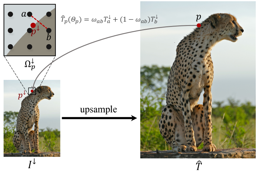
Figure 2. The proposed linear representation of high-resolution images. Each pixel $p$ in the high-resolution image is represented as the linear interpolation of two pixels $(a,b)$ in the low-resolution image, with $(a,b)$ and the interpolation weight optimized for minimizing the representation error.

Given an image operator $f$ and a high-resolution input image $I$ with RGB colors, our goal is to obtain an approximation $\hat{T}$ of the original output $T=f(I)$. With the guided upsampling method, we first apply $f$ to a downsampled image $I^{{}_{\downarrow}}$, and then upsample the result $T^{{}_{\downarrow}}$to the high-resolution output $\hat{T}$ with the guidance of $I$. We need to optimize the downsampling and upsampling processes in order to minimize the difference between $\hat{T}$ and $T$. Note that the same as previous universal guided upsampling methods (Kopf et al., 2007; Chen et al., 2016), we also treat $f$ as a black-box operator that is scale-invariant.

(a) Source (560$\times$560)

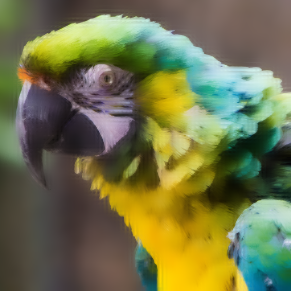
(b) JBU ($8\times$)

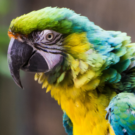
(c) GLU^∗ ($16\times$)

(d) GLU^∗ ($32\times$)

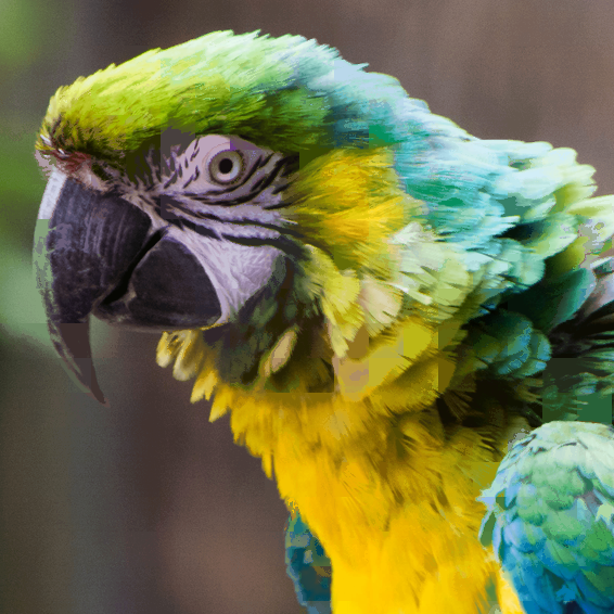
(e) GLU ($32\times$)

Figure 3. Guided self-upsampling with JBU and our method. The input source image is downscaled and then upsampled to the original resolution with the guidance of itself. GLU^∗ is our method as described in Section 3.1, GLU is the accelerated version introduced in Section 3.2. They both can well recover the original image for large ratios as $32\times$. As the comparison, JBU produces obvious blur even for smaller ratios as $8\times$.

3.1. Guided Linear Upsampling

We first assume that the downsampled input image $I^{{}_{\downarrow}}$ is given, or produced with regular grid downsampling by default. As illustrated in Figure 2, in order to optimize the upsampling, our basic assumption is that each pixel $p$ of the high-resolution target image $T$ can be well approximated by the linear interpolation of a pair of low-resolution pixels $(a,b)$ as follows:

(1) $$\hat{T}_{p}=\omega_{ab}T^{{}_{\downarrow}}_{a}+(1-\omega_{ab})T^{{}_{\downarrow}}_{b}\;\;s.t.\;\;a,b\in\Omega_{p^{{}_{\downarrow}}}$$

where $\omega_{ab}$ is the weighting function, $p^{{}_{\downarrow}}$ is the downscaled coordinates of $p$, and $\Omega_{p^{{}_{\downarrow}}}$ is a small neighborhood of $p^{{}_{\downarrow}}$. $\hat{T}_{p}$ is an estimate of the original output $T_{p}$. The above assumption can actually be derived from the well-known color line model (Levin et al., 2007), which we will explain in Section 4.1. Eq. (1) contains three parameters $a,b,\omega_{ab}$, which need to be optimized in order to minimize the upsampling error. Denote the parameters of pixel $p$ by $\Theta_{p}=\{a,b,\omega_{ab}\}$, and then $\Theta$ is a $3\times H\times W$ tensor containing the parameters of all pixels of $T$. Given $\Theta$, the corresponding high-resolution output $\hat{T}(\Theta)$ can be easily computed with Eq. (1).

The same as previous local color transformation methods (Levin et al., 2007; He et al., 2012; Chen et al., 2016), we also assume that the target image can be locally represented as the affine transformation of the source image. As will be explained in Section 4.1, in this case the source and target images can be optimally upsampled with the same set of parameters. In other words, if $\Theta$ is optimal for the source image, then it should be optimal for the target image as well. Therefore, the optimal parameters $\Theta$ can be solved w.r.t only the source image in order to minimize its upsampling error:

(2) $$\Theta=\mathop{\arg\min}\limits_{\Theta}\parallel\hat{I}(\Theta)-I\parallel$$

in which $\hat{I}(\Theta)$ is the upsampled source image with the given parameters $\Theta$. We assume that $\Theta_{p}$ of each pixel is independent of each other, so the above equation can be solved for each pixel as

(3) $$\Theta_{p}=\mathop{\arg\min}\limits_{\Theta_{p}}\parallel\omega_{ab}I^{{}_{\downarrow}}_{a}+(1-\omega_{ab})I^{{}_{\downarrow}}_{b}-I_{p}\parallel$$

which is a combinatorial optimization problem that is usually difficult to solve. Fortunately, in our case $\Omega_{p^{{}_{\downarrow}}}$ is a small neighborhood (a $3\times 3$ window in our experiments), so it is easy to enumerate all possible pixel pairs. For each selected pixel pair $(a,b)$, the optimal weighting parameter should be

(4) $$\omega_{ab}=\frac{(I_{p}-I^{{}_{\downarrow}}_{b})(I^{{}_{\downarrow}}_{a}-I^{{}_{\downarrow}}_{b})}{\parallel I^{{}_{\downarrow}}_{a}-I^{{}_{\downarrow}}_{b}\parallel^{2}+\varepsilon}$$

which makes the interpolation result $\hat{I}_{p}$ the projection of $I_{p}$ on the color line determined by $I^{{}_{\downarrow}}_{a}$ and $I^{{}_{\downarrow}}_{b}$, just as previous sampling-based matting methods (Wang and Cohen, 2007). $\varepsilon$ is a small constant ($10^{-3}$ in our implementation) to avoid dividing by zero in flat patches.

Figure 3 demonstrates an example to upsample an image from its downscaled counterpart. The above simple method achieves surprisingly good results. Even for large ratios such as $32\times$, details of the original image can be reconstructed almost perfectly. As a comparison, the result of JBU is obviously blurred even for smaller ratios. Note that for the methods based on the local color transformation (He et al., 2012; Chen et al., 2016), the above task is trivial because an identity transformation would be learned if the source and target images are the same.

(a) Source (112$\times$168)

(b) GNU

(c) GLU

Figure 4. Comparison of GLU and GNU for upsampling an image patch from its $8\times$ downsampling. GNU cannot represent the smooth variations of the original image, and thus produces obvious artifacts.

3.2. Efficient Computation

The complexity of the above method is quadratic to the number of pixels in $\Omega_{p^{{}_{\downarrow}}}$. For a typical $3\times 3$ window, it needs to check 36 pairs of pixels in order to minimize Eq. (3). For high-resolution images, this still requires a large amount of computation, so we propose the following improvements for better efficiency.

Firstly, we find that it is not necessary to enumerate all pixel pairs $(a,b)\in\Omega_{p^{{}_{\downarrow}}}$ in order to optimize Eq. (3). Instead, we can first fix $a$ as the pixel with the most similar color to $I_{p}$, and then optimize only $b$ and $\omega_{ab}$ with respect to Eq. (3). In this way, the complexity can be reduced to be linear with $|\Omega_{p^{{}_{\downarrow}}}|$. Since $a$ is close to $I_{p}$ in the color space, the approximation error should be small for the projection of $I_{p}$ on the color line.

Secondly, it is easy to see that if $I_{p}$ is on the color line determined by $I^{{}_{\downarrow}}_{a}$ and $I^{{}_{\downarrow}}_{b}$, the interpolation weight $\omega_{ab}$ as in Eq. (4) reduces to

(5) $$\omega_{ab}=\frac{\parallel I_{p}-I^{{}_{\downarrow}}_{b}\parallel}{\parallel I_{p}-I^{{}_{\downarrow}}_{a}\parallel+\parallel I_{p}-I^{{}_{\downarrow}}_{b}\parallel+\varepsilon}$$

which can be computed more efficiently and the results are guaranteed to be in $[0,\,1]$. Since the color lines not crossing $I_{p}$ are less likely to be selected, the above approximation has little impact on the quality of our method.

As shown in Figure 3, the above accelerations would not introduce noticeable differences compared to our original method, but the complexity is much lower. Therefore, in the following we will use the accelerated method by default.

Our final upsampling method is as described in the Algorithm 1. It is very simple and efficient. $\Omega_{p^{{}_{\downarrow}}}$ is typically chosen as a $3\times 3$ window, so for each pixel, only 9 pixel pairs need to be checked. Note that if we fix $\omega_{ab}$ to 1, then the optimization in line 3 is not necessary, and $\hat{T}_{p}$ would be equal to $T^{{}_{\downarrow}}_{a}$. We call this special case of our method as Guided Nearest Upsampling (GNU). As shown in Figure 4, GNU lacks the ability to recover the ramp edges and smooth variations of natural images, thus producing blocky effects and false contours, which can be effectively eliminated by using GLU.

Input: High-res source image $I$, low-res source image $I^{{}_{\downarrow}}$ and corresponding target image $T^{{}_{\downarrow}}$.

Output: High-res target image $\hat{T}$.

1

2for each pixel $p\in I$ do

3       Find $a$ as the pixel in $\Omega_{p}^{{}_{\downarrow}}$ with the most similar color to $I_{p}$ ;

4       Fix $a$ and optimize $b,\omega_{ab}$ with Eq. (3)(5);

5       Compute $\hat{T}_{p}$ as Eq. (1);

6      

7 end for

ALGORITHM 1 Efficient Guided Linear Upsampling.

(a) Source (284$\times$202)

(b) $16\times$ downsampling

(c) GLU^-

(d) Optimized downsampling

(e) GLU

Figure 5. Demonstration of downsample optimization. (a) The input image with some thin structures. (b) Most thin structures are lost with $16{\times}$ default downsampling. (c) The result upsampled from (b), the thin structures cannot be recovered. (d) Optimized $16{\times}$ downsampled image. (e) The result upsampled from (d), the thin structures are well recovered.

Figure 6. Illustration of the proposed downsample optimization method. For the input high-resolution image $I$, we initialize $I^{\downarrow}$ with regular grid downsampling, and then iteratively update $I^{\downarrow}$ by trying to add large-error pixels to it for minimizing the total upsampling error.

3.3. Downsample Optimization

For large downsampling ratio, isolated thin structures and small regions may be completely lost due to regular grid downsampling. In this case, it would be impossible for the upsampling process to recover the original content. Figure 5 demonstrates such a situation. Although downsampling optimization has been extensively studied, previous works mainly aim to avoid aliasing artifacts (Kopf et al., 2013; Oeztireli and Gross, 2015; Weber et al., 2016), which is different from our goal. Some super-resolution methods (Kim et al., 2018; Sun and Chen, 2020; Xiao et al., 2020) also jointly optimize their downscaling and upscaling processes, which however, are not well suited for the proposed GLU upsampler.

Given the GLU upsampler $\Psi(I^{{}_{\downarrow}},\Theta)$, we can formulate the downsampling process as an optimization problem aiming to minimize the self-upsampling error of the source image. In practice since $\Theta$ is unknown, the downsampling and upsampling need to be jointly optimized as

(6) $$I^{{}_{\downarrow}},\Theta=\mathop{\arg\min}\limits_{I^{{}_{\downarrow}},\Theta}\parallel I-\Psi(I^{{}_{\downarrow}},\Theta)\parallel$$

with each pixel of $I^{{}_{\downarrow}}$ from exactly one pixel of $I$. Note that this is different from previous downsampling optimization methods, in which each pixel of $I^{{}_{\downarrow}}$ is usually filtered from multiple pixels of $I$ in order to reduce aliasing artifacts. For our method, the filtering in downsampling may significantly blur the upsampled image because it would shrink the endpoints of color lines, which is detrimental to image details.

Eq. (6) can be solved by iteratively optimizing $I^{{}_{\downarrow}}$ and $\Theta$. Given $I^{{}_{\downarrow}}$, the upsampling parameters $\Theta$ can be solved as in Algorithm 1. To optimize the downsampling, we first compute the pixel-wise error map $E,E_{p}=\parallel I_{p}-\hat{I}_{p}\parallel$. Obviously, the pixels with large error must be those that cannot be well represented by $I^{{}_{\downarrow}}$, and thus need to be added to $I^{{}_{\downarrow}}$ by replacing some existing pixels. Note that since each pixel in $I^{{}_{\downarrow}}$ may be used to interpolate multiple pixels of $I$, the above operation may not reduce the total error. Therefore, we adopt a trial-and-error approach, and if replacing some pixels in $I^{{}_{\downarrow}}$ does not reduce the total error, the replaced pixels would be rolled back.

Figure 6 illustrates the procedure of our method, more details are described in Algorithm 2. The trial-and-error procedure is executed for each connected region $C_{i}$ of pixels with large error ($\mathcal{E}$). The pixels with large errors are tried to be added to the downsampled image, and the operation would be accepted if it can reduce the total error, otherwise it would be unrolled. For multiple high-resolution pixels $[q^{{}_{\uparrow}}]$ mapped to the same low-resolution pixel location $q\in I^{{}_{\downarrow}}$, the one with the largest error would be selected to replace the original color of $q$.

As shown in Figure 5, the above method can effectively prevent the missing of thin structures and small regions. In most cases, it requires only 1 or 2 iterations to converge, and after the initialization, only pixels with large errors are involved for further processing, so only a little more computation is required.

Input: High-res source image $I$, the error threshold $\tau$, the maximum iterations $N$.

Output: Optimized low-res image $I^{{}_{\downarrow}}$ and upsampling parameters $\Theta$.

1

2Initialize $I^{{}_{\downarrow}}$ with regular grid downsampling;

3 Initialize $\Theta$ from $I,\;I^{{}_{\downarrow}}$ with Algorithm 1;

4 Compute initial error map $E$;

5 for n = 1, …, N do

6       Find the set of pixels with large error: $\mathcal{E}=\{p\,|\,E_{p}>\tau\}$ ;

7       if $\mathcal{E}$=$\emptyset$ then

8            Break

9       end if

10      Cluster $\mathcal{E}$ as connected components $C_{1},\cdots,C_{M}$;

11       for $i=1,\cdots,M$ do

12             Backup $\Theta,I^{{}_{\downarrow}},E$ for scroll back;

13             Compute $e^{0}=\sum_{p\in C_{i}}E_{p}$;

14             $Q=\{q\,|\,q\in I^{{}_{\downarrow}}\,\&\,[q^{{}_{\uparrow}}]\bigcap C_{i}\neq\emptyset$};

15             for $q\in Q$ do

16                   Update $I^{{}_{\downarrow}}_{q}$ with $I_{p},\;p=\mathop{\arg\max}\limits_{p\in[q^{{}_{\uparrow}}]\bigcap C_{i}}E_{p}$

17             end for

18            for $p\in C_{i}$ do

19                   Update $\Theta_{p}$ as in Algorithm 1;

20                   Update $E_{p}$ with updated $\Theta_{p}$;

21                  

22             end for

23            Compute $e^{1}=\sum_{p\in C_{i}}E_{p}$;

24             if $e^{1}>e^{0}$ then

25                   Scroll back updated regions of $\Theta,I^{{}_{\downarrow}}$ and $e$;

26                  

27             end if

28            

29       end for

30      

31 end for

32

ALGORITHM 2 Joint Optimization of Down- and Upsampling.

4. Analysis

An ideal guided upsampling method should be able to preserve the detail effects of the target image while avoiding artifacts such as bleeding and blurring. In the following we will analyze the capabilities of our method and show how it relates to previous methods.

4.1. Theoretical Derivation

The proposed upsampling method in Section 3.1 can be derived from the color line model (Levin et al., 2007) and local color transformation methods (Levin et al., 2007; He et al., 2012; Chen et al., 2016).

The color line model tells us that the colors of pixels in a small patch should be roughly on the same line in the color space. Therefore, the color of each pixel in the patch must be well approximated by the linear interpolation of the two endpoints $[a,b]$ of the color line. After downsampling, it can be expected that $[a,b]$ still can be well represented by two pixels in the downsampled patch, because of the information redundancy in the high-resolution image. As a result, each pixel color in the original patch can also be linearly interpolated by two pixels in the downsampled patch, as in Eq. (1).

The local color transformation methods assume that the output image can be locally represented as the affine transformation of the input image, i.e. $T_{p}=A_{p}I_{p}$, where $A_{p}$ is an affine transformation that varies smoothly over the image space. In addition, we require the operator to be approximately scale-invariant: $T^{{}_{\downarrow}}_{p}=A_{p}I^{{}_{\downarrow}}_{p}$. Therefore, if using $\Theta_{p}$ can linearly interpolate $I_{p}$, i.e.

(7) $$I_{p}=\omega_{ab}I^{{}_{\downarrow}}_{a}+(1-\omega_{ab})I^{{}_{\downarrow}}_{b}$$

then it immediately follows that

(8) $$T_{p}=\omega_{ab}A_{p}I^{{}_{\downarrow}}_{a}+(1-\omega_{ab})A_{p}I^{{}_{\downarrow}}_{b}=\omega_{ab}T^{{}_{\downarrow}}_{a}+(1-\omega_{ab})T^{{}_{\downarrow}}_{b}$$

which means that using $\Theta_{p}$ also can linearly interpolate $T_{p}$, as we have assumed in Section 3.1.

4.2. Edge Recovery

Typical image edges can be classified into three types: step edge, ramp edge, and roof edge (Koschan and Abidi, 2005; Yin et al., 2019). For natural images, most edges should be ramp edges connecting two regions. Obviously, the transition effects of ramp edges can be well represented by linear interpolation of the two region colors. Therefore, by interpolating only two pixels, GLU can recover the edges of the original image very well. As a comparison, using GNU can recover only the step edges, and thus would introduce significant artifacts, as is shown in Figure 4.

A natural question is whether we can achieve further improvements by interpolating more pixels. Indeed, Eq. (1) can be more generally expressed as

(9) $$\hat{T}_{p}=\sum\limits_{q\in\Omega_{p^{{}_{\downarrow}}}}\omega_{q}\;T^{{}_{\downarrow}}_{q}$$

with $\omega_{q}$ as the normalized weights. Interestingly, this is exactly the form of JBU. However, in JBU $\omega_{q}$ is not optimized, and the filtering effect would result in blur and edge reversal artifacts (He et al., 2012). It is easy to see that when $\sigma_{d}\to\infty$ and $\sigma_{r}\to 0$, JBU will reduce to GNU. However, in practice this is hard to achieve due to the numerical problems of the exp weighting function. By decreasing $\sigma_{r}$, the blurring artifacts of JBU can be reduced, but may lead to aliasing artifacts as GNU. Therefore, in this sense both GLU and GNU can be taken as special cases of JBU with optimized weights.

Although not tested, we do not see the need to take more pixels for interpolation. Involving more pixels not only makes the optimization more difficult, but may also lead to overfitting and extrapolation, both of which can reduce the result quality.

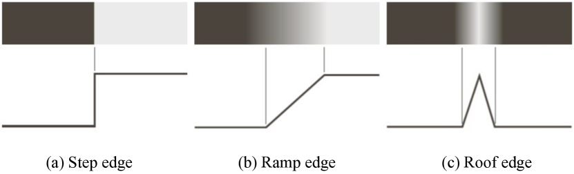
Figure 7. The three types of edges in natural images.

4.3. Detail Preservation

As discussed in Section 4.1, our method implicitly takes advantage of the local color transformation for transferring the upsampling parameters. However, it should be noted that unlike previous approaches such as guided filter (He et al., 2012) and BGU (Chen et al., 2016), our method does not require the transformations to be smooth in either image space or bilateral space. Therefore, it can better preserve the detail effects of the target image while avoiding the bleeding artifacts caused by over-smoothing.

One potential issue with our method is the lack of an explicit smoothness constraint. Although preserving smoothness is important for most image processing operators, we find that our method which operates on each pixel independently also works well in most situations. This is mainly because the linear interpolation model can well approximate the appearance of the original source image, which serves as a smooth guidance map that can suppress unsmooth artifacts if the target image has similar local affinities as the source image. However, if the pixel affinities of the source and target images are significantly different (e.g., when new edges are introduced in the target image), unsmooth artifacts may be produced. Actually, this is the main limitation of our method, which we will discuss further in Section 6.

5. Experiments

In experiments we evaluate the proposed method in various image processing applications, and compare it qualitatively and quantitatively with previous methods. We also demonstrate the advantages of our method for interactive image editing and real-time video processing, and reveal its limitations for more diverse applications.

Table 1. Comparisons of different methods with PSNR scores. The low-resolution target is produced from the low-resolution source using the image operator, except the applications with ^†, for which the low-resolution target is obtained by downsampling the reference image.

PSNR$\uparrow$	alpha matting		colorization		unsharp mask		$L_{0}$-smoothing		dehazing		laplacian filter		unsharp mask†
	$8\times$	$16\times$	$8\times$	$16\times$	$8\times$	$16\times$	$8\times$	$16\times$	$8\times$	$16\times$	$8\times$	$16\times$	$8\times$	$16\times$
JBU	25.6	22.9	20.9	20.1	18.2	16.9	22.3	20.1	25.9	22.3	15.6	13.8	19.0	17.8
BGU-fast	21.4	22.2	28.5	27.8	23.8	23.2	22.8	22.2	21.1	17.7	21.8	21.3	25.1	24.9
BGU	28.3	25.8	30.7	28.8	23.5	22.4	27.0	25.4	26.8	23.4	23.7	22.3	25.4	25.0
GLU-	31.4	28.9	29.7	27.7	23.6	22.3	23.6	24.5	27.6	24.1	20.5	17.2	25.2	24.0
GLU	31.5	29.1	31.3	29.6	24.0	22.4	28.8	27.1	27.6	24.1	23.1	24.5	25.9	25.2

Table 2. Comparisons of different methods with SSIM scores.

SSIM$\uparrow$	alpha matting		colorization		unsharp mask		$L_{0}$-smoothing		dehazing		laplacian filter		unsharp mask†
	$8\times$	$16\times$	$8\times$	$16\times$	$8\times$	$16\times$	$8\times$	$16\times$	$8\times$	$16\times$	$8\times$	$16\times$	$8\times$	$16\times$
JBU	0.93	0.91	0.60	0.56	0.40	0.36	0.80	0.78	0.91	0.88	0.32	0.27	0.41	0.37
BGU-fast	0.71	0.64	1.00	1.00	0.85	0.84	0.83	0.82	0.79	0.72	0.82	0.81	0.77	0.75
BGU	0.86	0.78	1.00	1.00	0.88	0.85	0.88	0.84	0.90	0.85	0.88	0.84	0.79	0.77
GLU-	0.96	0.94	0.97	0.97	0.86	0.83	0.86	0.83	0.94	0.89	0.80	0.68	0.82	0.79
GLU	0.96	0.94	0.99	0.99	0.87	0.83	0.89	0.85	0.94	0.89	0.85	0.80	0.83	0.81

5.1. Comparisons

For quantitative evaluations we tested our method with the following applications and datasets:

$\bullet$ Alpha Matting with the method of (Chen et al., 2013). The dataset is from (Rhemann et al., 2009), which consists of 27 high-resolution images with a size of about $6-8$M pixels.

$\bullet$ Colorization with the method of (Levin et al., 2004). The dataset is from the high-quality 2K images for super-resolution (Agustsson and Timofte, 2017). We use all 100 images in the validation set. The source grayscale images are produced by graying the original RGB images and then converted to 3 channels simply by replicating the channel. The required seed constraints (Levin et al., 2004) are sparsely sampled from the original color images.

$\bullet$ Dehazing with the method of (Li et al., 2017). The dataset is from NTIRE-19 benchmark (Ancuti et al., 2019), which includes 55 real hazy images with $\sim$2M pixels.

$\bullet$ Unsharp Masking for enhancing image details by the method of (Ngo et al., 2020). The source images are the same as colorization.

$\bullet$ $L_{0}$ Smoothing using the method of (Xu et al., 2011). The dataset is the same as the colorization.

$\bullet$ Laplacian Filtering for enhancing image details with the method of (Aubry et al., 2014). The dataset is the same as colorization.

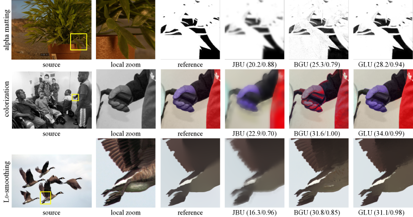
Figure 8. Visual comparisons of different methods with $8\times$ downsampling. In the parentheses are the PSNR/SSIM scores.

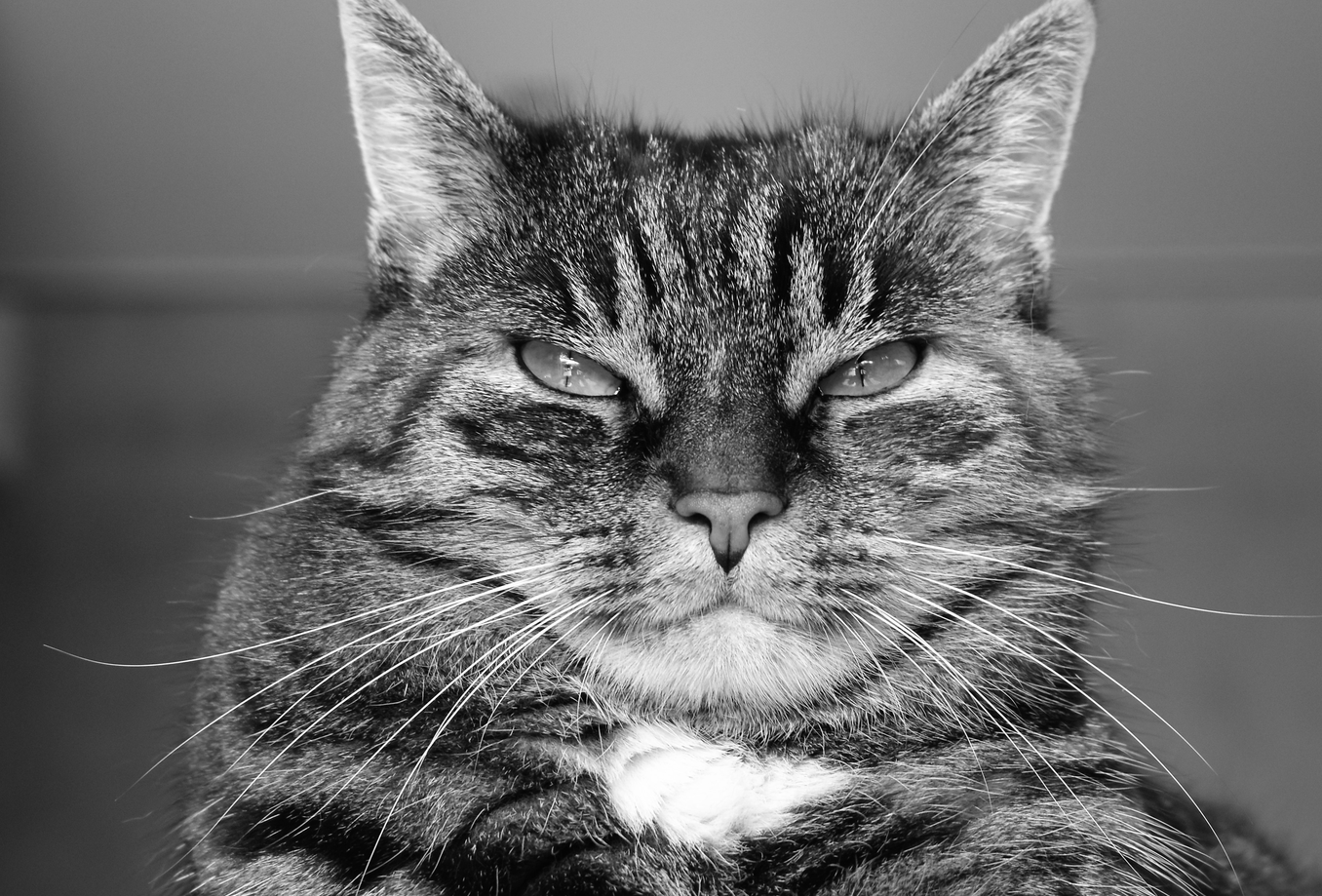
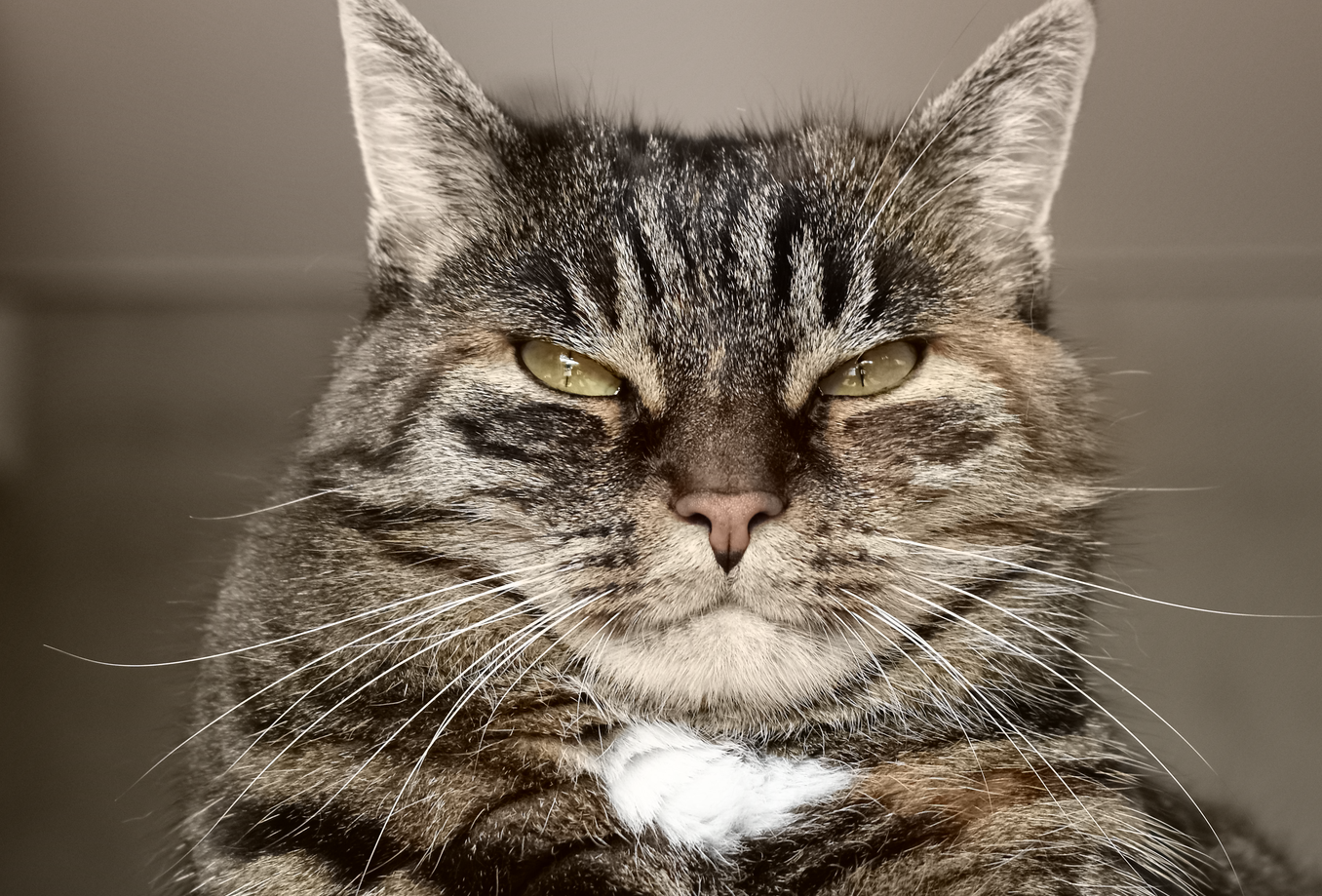
(a) source (1356$\times$919)	(b) reference
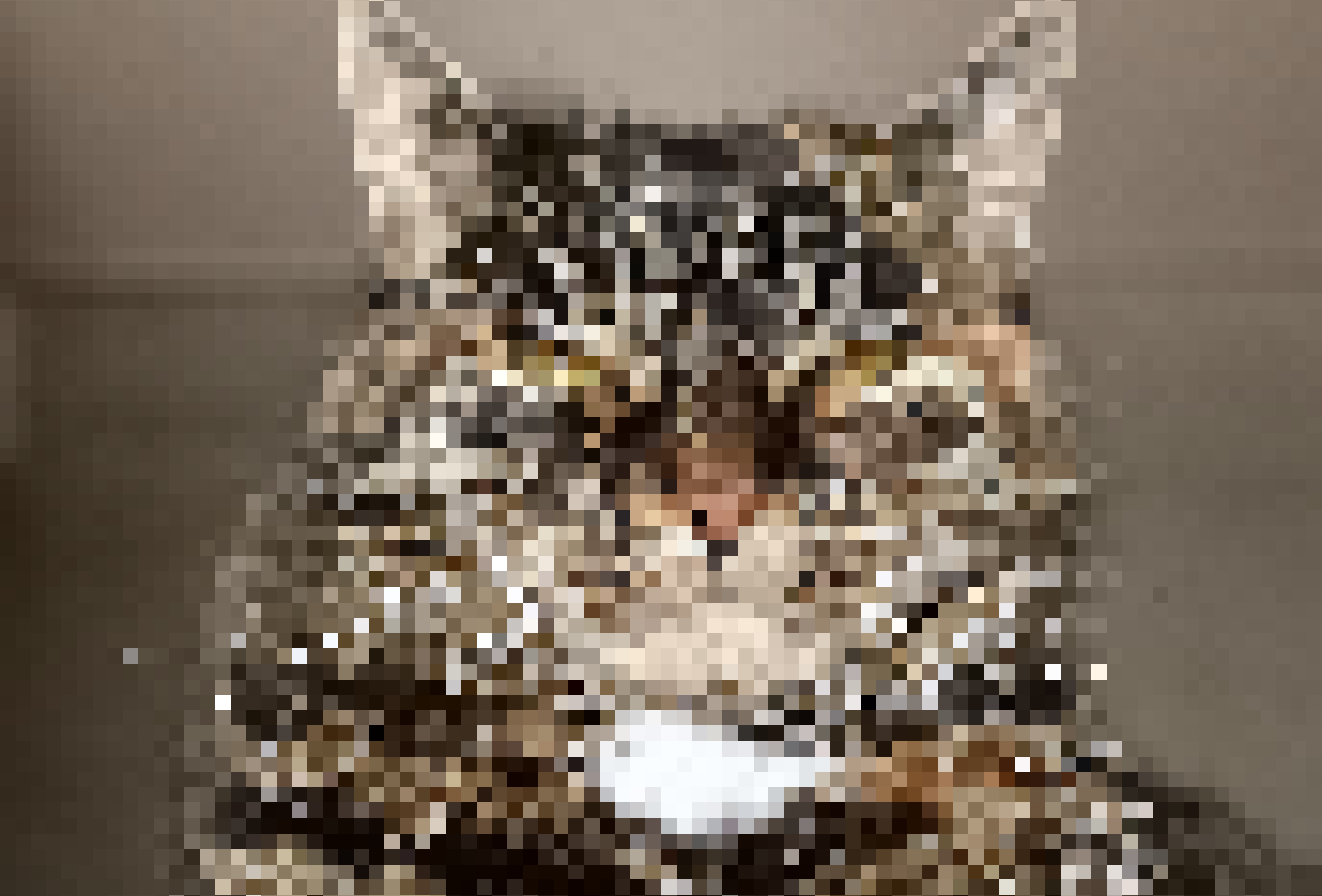
(c) low-res target of GLU-	(d) GLU-
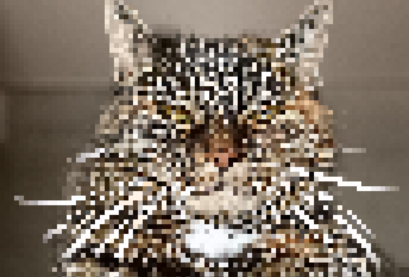
(e) low-res target of GLU	(f) GLU

Figure 9. The effect of downsampling optimization demonstrated on colorization at 16$\times$. GLU can better preserve fine image structures (the cat whiskers) than GLU^-.

The low-resolution target images are produced from the downsampled source images using the chosen image operators, and then upsampled using our technique to produce the full-resolution target images. Table 2 and Table 2 are the quantitative results with PSNR and SSIM scores, respectively. PSNR measures the difference in pixel values, while SSIM mainly measures the similarity of local structures. We compare our method with JBU (Kopf et al., 2007) and BGU (Chen et al., 2016). For JBU, we use the default parameter setting with $5\times 5$ support windows and $\sigma_{d}=0.5,\sigma_{r}=0.1$. For BGU we test both the global method with the authors’ MATLAB code, and the fast local method (BGU-fast) implemented with Halide (Ragan-Kelley et al., 2012, 2013). For GLU we use the default setting as described in Section 5.2. GLU^- is our method without downsampling optimization.

For most applications our method outperforms JBU and BGU for both scores. Figure 8 shows some examples. In general, for large scaling ratios such as $8\times$ and $16\times$, JBU tends to overblur low-contrast edges, while BGU tends to produce bleeding artifacts that mix the effects of different regions due to the smooth constraint of local transformations, as we analyzed in Sections 4.2 and 4.3.

Since BGU represents the target image as the local transformations of the source image, it is good at preserving the source image structures, and is therefore advantageous for applications such as Colorization, Unsharp Masking, and Laplacian Filter. For these applications BGU achieves better SSIM scores than our method. In particular, for Colorization, BGU obtains a full SSIM score, because our colorization method modifies only the chrominance channels, while SSIM is computed using only the grayscale channel. However, the PSNR scores of these applications are still comparable to or lower than our method. For applications where some source details need to be removed, such as Matting and Smoothing, preserving the local structures of the source image may have unwanted effects, e.g. for image smoothing BGU may re-introduce some source details that have been removed by the smoothing operator, as demonstrated in Figure 8. For these applications our method can significantly outperform BGU.

The downsample optimization can improve the PSNR and SSIM scores for all tested applications. As shown in Figure 9, fine image structures can be better preserved with the optimized downsampling. In comparison with the regular grid downsampler, the optimized downsampler may result in more gritty and aliased low-resolution images due to the irregular spatial sampling. However, note that such aliasing actually can improve the upsampled image because the joint optimization only accepts results with lower upsampling errors. Moreover, for operators that can preserve local affinities (as assumed by our method), the low-resolution target image should have the same aliasing as the downsampled source image, which should be beneficial for the upsampled target image according to our analysis in Section 4.

For Unsharp Masking, it is strange that BGU-fast performs better than BGU in terms of PSNR. Actually, this is caused by the different effects of the image operator at different scales. As shown in Figure 10, the upsampled results of BGU and GLU are largely different from the reference, which is obviously caused by the image operator rather than the upsampler. In this case, we consider the scores to be mostly noise and not trustworthy for the evaluation. The last column of Tables 2 and 2 shows the results with low-resolution target downsampled from the reference, which can better reflect the net effect of upsampling methods.

Finally, to see the effect of our method for large ratio of upsampling, we conducted experiments with larger ratios of $32\times$, $64\times$, and even $128\times$. Figure 11 shows an example for matting. Surprisingly, for the tested image, even for $128\times$ of downsampling and upsampling, our method still obtains pretty good results, which are better than the results of JBU and BGU with smaller ratios.

(a) source	(b) reference
(c) BGU	(d) GLU

Figure 10. Unsharp Masking with $8\times$ downsampling. The results of BGU and GLU are comparable, and both look better than the reference.

(a) Source ($3270\times 2388$)	(b) BGU 32$\times$	(c) BGU 64$\times$	(d) JBU 32$\times$
(e) Reference	(f) GLU 32$\times$	(g) GLU 64$\times$	(h) GLU 128$\times$

Figure 11. Experiments with large ratios of downsampling and upsampling. JBU produces obvious blur for $32\times$, BGU produces significant bleeding for $64\times$, and our method gets pretty good results even for $128\times$. For this experiment the low-resolution target images are downsampled from the reference, in order to observe the net effect of upsampling methods.

5.2. Parameters

Our method contains only 3 parameters, i.e. the window size $S$ of $\Omega_{p^{{}_{\downarrow}}}$, the error threshold $\tau$ and the maximum number of iterations $N$. $\tau$ should be an error value that may introduce noticeable visual difference, and for most examples our joint optimization requires only 1 or 2 iterations to remove large-error regions, so the parameters are easy to set. In our experiments, they are fixed to $S=3$, $\tau=30/255$, $N=3$.

Table 3. Effect of the window size $S$ to the resulting quality in PSNR.

window size	$3\times 3$	$5\times 5$	$7\times 7$	$9\times 9$
self-upsampling	41.31	42.83	44.04	44.92
matting	35.47	35.18	34.76	34.15
colorization	32.39	29.95	29.94	28.74

Table 3 investigates the effect of the window size $S$. Using a larger window size can lead to better self-upsampling, but slightly reduces the quality of the target images. Actually, a $3\times 3$ window in the downscaled image corresponds to a large enough neighborhood in the original resolution, so using a larger window size is not necessary and may degrade performance around low-contrast edges.

Compared with JBU and BGU, the parameter setting of our method is much simpler. This advantage makes it more suitable to be used as a universal guided upsampler for different situations.

Table 4. Time cost (ms).

Image Size	JBU	BGU	BGU-fast	GLU	GLU-
	C++	Matlab	Halide	C++	CUDA
2K	364	5772	13.1	125	5.6
4K	1427	18029	28.5	507	14.3

5.3. Time Cost

Table 4 compares the time cost of different methods. The BGU global method implemented with MATLAB is slow to compute, JBU and GLU are much faster, but still cannot reach real-time speed. BGU-fast implemented with Halide can be very fast even on CPU, but as compared in Tables 2 and 2, its quality is significantly lower than our method because the local method is unstable in some situations.

The main computation of our method is the joint optimization of $\Theta$ and $I^{{}_{\downarrow}}$. Note that since each pixel is optimized independently, our method is parallelizable and can be greatly accelerated with GPU. For a test we implemented GLU^- with CUDA and tested it on a laptop with Nvidia GTX1650 GPU. The accelerated version takes only about 5ms for 2K images and 14ms for 4K images, so it can be easily incorporated for real-time video processing.

A great advantage of our method is that the joint optimization process is target-free, i.e. the optimization is independent of the target image. Therefore, it can be precomputed before the target image is acquired, as we will demonstrate in Sections 5.4 and 5.5. For applications where multiple operators may be applied for the same image, optimized parameters can be cached and shared between different operators, which further reduces the overall computations of our method.

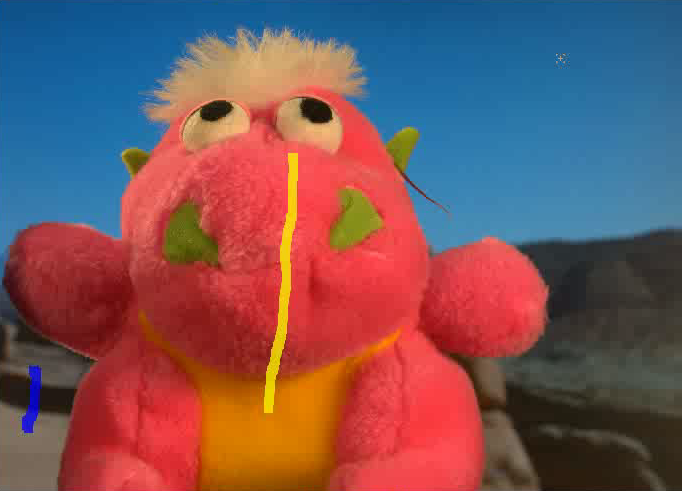
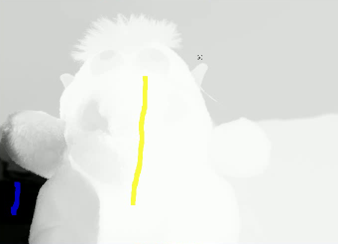
(a)	(b)
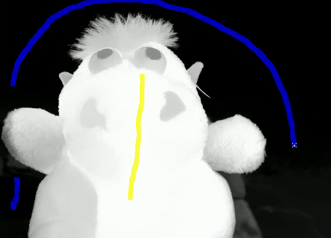
(c)	(d)

Figure 12. Interactive matting with instant feedback. (a) input image with initial scribble brushes. (b) the initial alpha matte. (c)(d) the changes in alpha matte can be observed instantly while the user moving mouse to add a new brush.

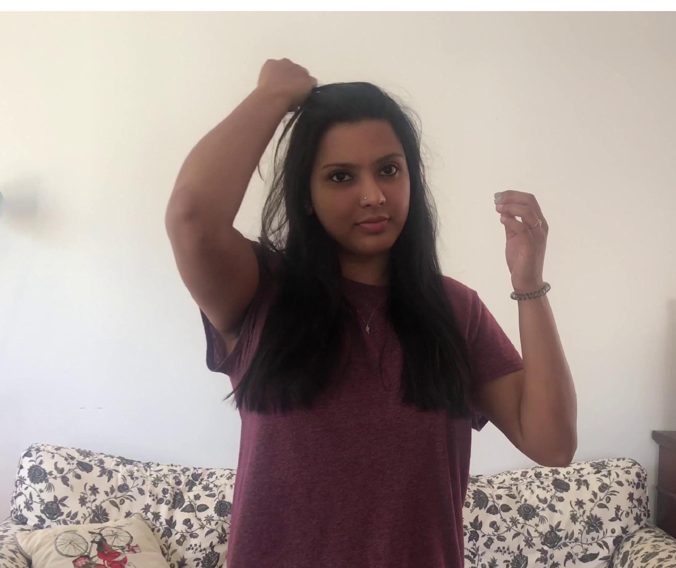
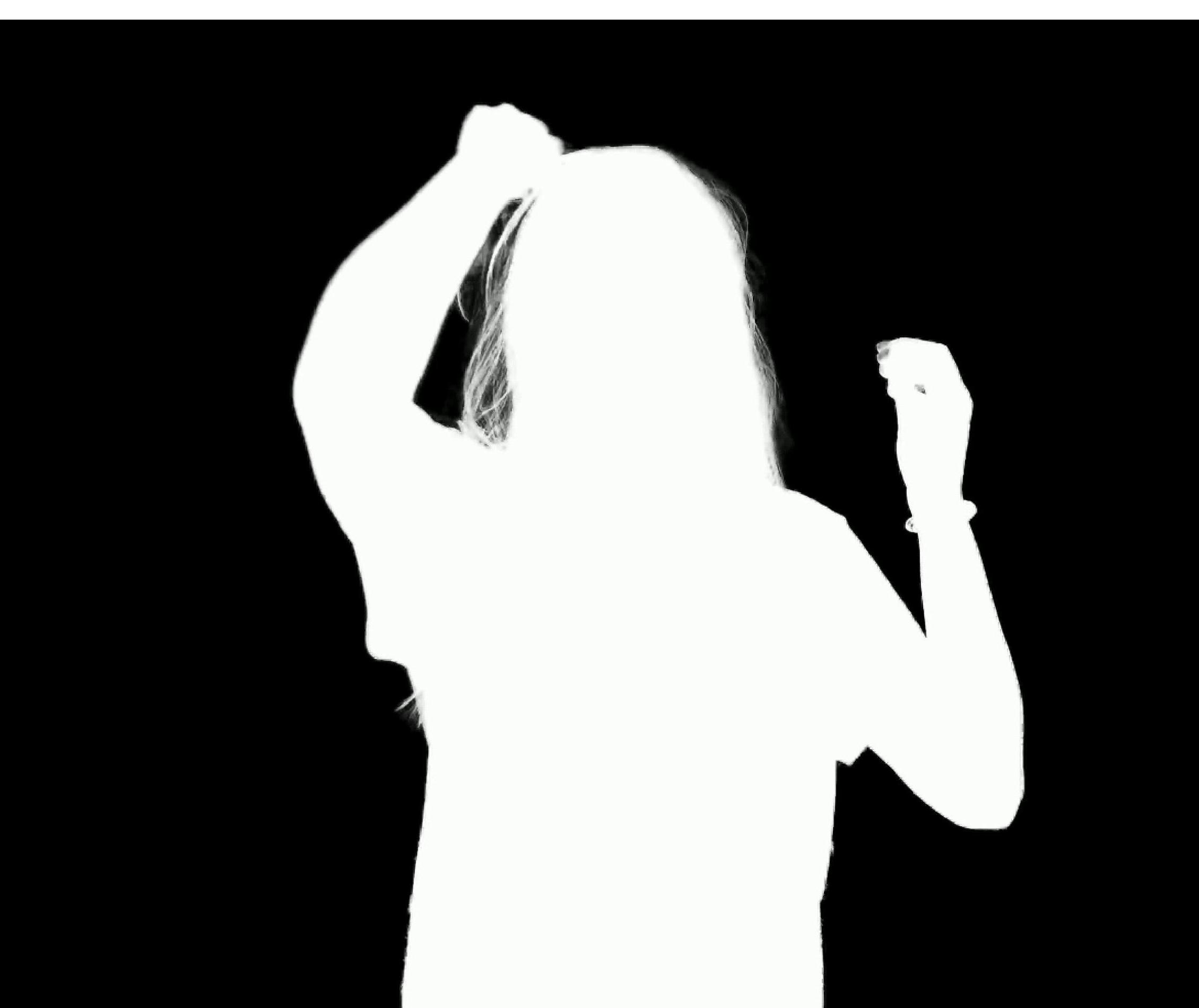
(a) Source (3840$\times$2160)	(b) full res. (¡5fps)
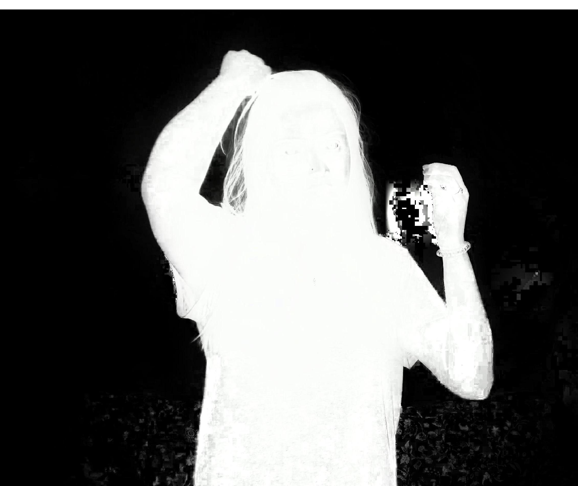
(c) BGU-fast $8\times$ ($\sim$20fps)	(d) GLU${}^{-}8\times$ (¿30fps)

Figure 13. Real-time video matting with BackgroundMattingV2 (Lin et al., 2021), which can achieve only less than 5fps with GTX1650 GPU. With the acceleration of our method, it can easily achieve real-time speed.

5.4. Interactive Editing with Instant Feedback

As mentioned above, the joint optimization process is target-free, so it can be precomputed for interactive image editing. The optimized upsampling parameter $\Theta$ can be stored as a $3\times H\times W$ tensor. Given $\Theta$, the upsampling requires only a simple linear interpolation for each pixel, whose computation is negligible for interactive applications.

As a demonstration, we built an interactive matting system that enables instant feedback without GPU acceleration. It is known that automatic image matting is very hard for general objects, while interactive matting requires fast speed for better user experience. To demonstrate the power of the proposed approach, we adopted the global matting method proposed in (Levin et al., 2007), which needs to solve a large sparse linear system, and is therefore very slow for large images.

Regardless of the size of the input image, our system resizes it to a small image of no more than 10K pixels, for which the matting method is invoked and then the result matte is upsampled to the full resolution for display. Thus, the main computation is to solve the $10000\times 10000$ sparse linear system. We adopted the MKL PARDISO solver, which is very efficient and requires about 0.5 seconds for each solution. Surprisingly, although 10K pixels seems very small, we find it works well with the proposed guided upsampling method. Actually, as shown in Figure 11, our method can achieve good results for very large ratios such as $64\times$ and $128\times$. For a typical high-resolution input of 10M pixels, downsampling it to 10K requires a downscale ratio about $30\times$, which is not too large in comparison. After a period of user interaction, a trimap can be estimated from the current alpha matte, then our system proceeds with unknown pixels at a finer scale. In this way, the matting operator is invoked from coarse to fine, which helps avoid upsampling errors due to large ratio of downsampling.

Figure 12 demonstrates the effectiveness of our system. The user can instantly observe changes in the matting result when moving the mouse for editing. This enables the user to add brushes accordingly in the areas with large errors, thus greatly improving efficiency and bringing a much better user experience. Please see the supplementary material for video demonstrations.

5.5. Real-time Video Processing

Our method is parallelable and can be executed fast with GPU implementation, thus enabling real-time video processing. To demonstrate this, we apply our method to BackgroundMattingV2 (Lin et al., 2021), an efficient video matting method that can achieve 30fps for 4K videos on RTX2080ti GPU. However, for our low-end test machine with GTX1650 GPU, it requires more than 200ms for each frame. To achieve real-time speed, we apply our method with 8$\times$ downsampling, then the low-resolution matting with BackgroundMattingV2 requires about 21ms, and upsampling with GLU^- requires about 14ms, so in total it takes about 35ms per frame.

The target-free property of our method can further improve the efficiency. Since the optimization of GLU^- is independent of the matting result, it can be executed in parallel with the matting procedure. In this way the time cost can be further reduced. Compared to the results in full resolution, the sacrifice in quality is usually small for 8$\times$ downsampling, as shown in Figure 13. In comparison with BGU-fast, our method can achieve faster speed and better quality.

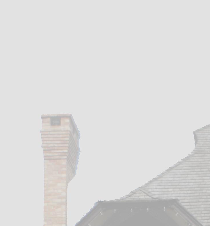
(a) Source

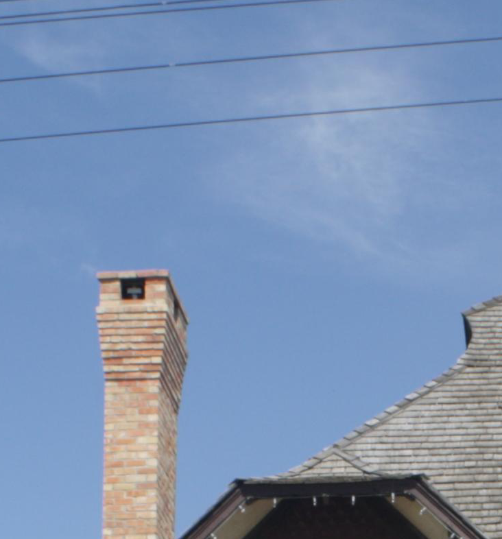
(b) Reference

(c) GLU $8\times$

Figure 14. Failure case of our method. New edges not appear in the source image cannot be well recovered.

(a) Source

(b) Reference

(c) GLU $8\times$

Figure 15. Our method may produce unsmooth artifacts when the source and target images have very different pixel affinities.

Figure 16. Examples of CycleGAN style transfer (Zhu et al., 2017), which may introduce dramatic changes to local image structures. In this case, our method may produce unsmooth artifacts, while BGU may smooth out the new structures. Since CycleGAN can only output 256$\times$256 fixed-size results, the reference here is the low-resolution target image.

6. Limitations

The same as JBU and BGU, a basic assumption of our method is that the source and target images have almost the same local affinity, i.e. pixels with more similar color in the source image should have more similar color in the target output. Therefore, our method is not suitable for applications that may introduce new edges in the target image. Figure 14 shows such an example. The affinity of new edges differs a lot from the source and is therefore out of the scope of joint optimization. In a more general case, our method may produce unsmooth edges due to different local affinities. As shown in Figure 15, since the object has similar color to the background, our method fails to accurately recover the sharp matte edges.

Note that unlike adding new edges, removing edges does not usually cause problems for our method, because the resultant pixels can still be interpolated by neighboring pixels, so applications such as matting and smoothing can be well supported. In contrast, BGU may insistent on preserving the edges and local structures of the source image, so for edge-removing applications it may produce artifacts, as demonstrated in Figure 8.

Due to the limitation on handling new edges, our method is not suitable for applications that may drastically change the local image structures, such as the recent learning-based style transfer methods (Zhu et al., 2017; Park et al., 2020). This is a common limitation for universal guided upsampling methods including JBU and BGU. Figure 16 shows some examples. As shown, for cases such as Horse2Zebra, BGU may completely ignore new edges, while our method results in unsmooth artifacts. In fact, since for new edges, there is no guidance information in the source image, it is not able to get good results without any domain-specific prior knowledge, so using learning-based approaches should be better in this case.

For real applications, a practical issue is to find an image operator that is suitable for low-resolution processing. As demonstrated in Figure 10, the input image scale may have a great effect on the output of some image processing methods. For example, we found that BackgroundMattingV2 produces significantly more errors when being applied to $8\times$ downsampling inputs, because it is originally designed for high-resolution video. Another example is optical flow estimation (Teed and Deng, 2020), whose accuracy is greatly influenced by image resolution and requires special treatment after upsampling. How to adapt these methods for better low-resolution image processing is a remaining problem.

7. Conclusion

We propose a simple yet effective guided upsampling method, which represents each high-resolution pixel as a linear interpolation of two low-resolution pixels. Transition edges and smooth variations in natural images can be well represented. The upsampling parameters and the downscaled input image are jointly optimized in order to minimize the upsampling error. We reveal and discuss the connections with previous methods. In particular, our method can be considered as a special case of JBU with optimized weights, and it also implicitly exploits pixel-level local color transformations. These properties enable it to overcome the blurring and bleeding artifacts of previous approaches.

We demonstrate the advantages of our method with a wide range of image operators. For interactive editing tasks, our approach enables time-costly operators to achieve instant feedback without hardware acceleration. Real-time video processing can also be enabled easily for high-resolution inputs. Finally, our work shows that a high-resolution image can be well represented by simple linear interpolation of its downscaled counterpart. Similar to bilateral filter and local color transformations, the power of such representation can be further explored in related tasks such as learning-based image processing (Gharbi et al., 2017), super resolution (Sun and Chen, 2020), segmentation (Mazzini, 2018), etc.

8. Acknowledge

The authors would like to thank the anonymous reviewers for their valuable comments and suggestions. This work is supported by National Key R&D Program of China under grant (2022YFB3303200), Natural Science Foundation of China (62072284), and Center-initiated Research Project of Zhejiang Lab (2021NB0AL01).

References

- (1)
- Agustsson and Timofte (2017) Eirikur Agustsson and Radu Timofte. 2017. NTIRE 2017 Challenge on Single Image Super-Resolution: Dataset and Study. In The IEEE Conference on Computer Vision and Pattern Recognition (CVPR) Workshops.
- Ancuti et al. (2019) Codruta O Ancuti, Cosmin Ancuti, Radu Timofte, Luc Van Gool, Lei Zhang, and Ming-Hsuan Yang. 2019. Ntire 2019 image dehazing challenge report. In Proceedings of the IEEE/CVF Conference on Computer Vision and Pattern Recognition Workshops. 0–0.
- Aubry et al. (2014) Mathieu Aubry, Sylvain Paris, Samuel W Hasinoff, Jan Kautz, and Frédo Durand. 2014. Fast local laplacian filters: Theory and applications. ACM Transactions on Graphics (TOG) 33, 5 (2014), 1–14.
- Barron et al. (2015) Jonathan T Barron, Andrew Adams, YiChang Shih, and Carlos Hernández. 2015. Fast bilateral-space stereo for synthetic defocus. In Proceedings of the IEEE Conference on Computer Vision and Pattern Recognition. 4466–4474.
- Bousseau et al. (2009) Adrien Bousseau, Sylvain Paris, and Frédo Durand. 2009. User-assisted intrinsic images. In ACM SIGGRAPH Asia 2009 papers. 1–10.
- Chai et al. (2022) Lucy Chai, Michaël Gharbi, Eli Shechtman, Phillip Isola, and Richard Zhang. 2022. Any-Resolution Training For High-Resolution Image Synthesis. In Computer Vision – ECCV 2022: 17th European Conference, Tel Aviv, Israel, October 23–27, 2022, Proceedings, Part XVI. Springer-Verlag, Berlin, Heidelberg, 170–188.
- Chen et al. (2016) Jiawen Chen, Andrew Adams, Neal Wadhwa, and Samuel W Hasinoff. 2016. Bilateral guided upsampling. ACM Transactions on Graphics (TOG) 35, 6 (2016), 1–8.
- Chen et al. (2013) Qifeng Chen, Dingzeyu Li, and Chi-Keung Tang. 2013. KNN matting. IEEE transactions on pattern analysis and machine intelligence 35, 9 (2013), 2175–2188.
- Dai et al. (2021) Yutong Dai, Hao Lu, and Chunhua Shen. 2021. Learning Affinity-Aware Upsampling for Deep Image Matting. In Proceedings of the IEEE/CVF Conference on Computer Vision and Pattern Recognition. 6841–6850.
- Durand and Dorsey (2002) Frédo Durand and Julie Dorsey. 2002. Fast bilateral filtering for the display of high-dynamic-range images. In Proceedings of the 29th annual conference on Computer graphics and interactive techniques. 257–266.
- Farbman et al. (2008) Zeev Farbman, Raanan Fattal, Dani Lischinski, and Richard Szeliski. 2008. Edge-preserving decompositions for multi-scale tone and detail manipulation. ACM Transactions on Graphics (TOG) 27, 3 (2008), 1–10.
- Gharbi et al. (2017) Michaël Gharbi, Jiawen Chen, Jonathan T Barron, Samuel W Hasinoff, and Frédo Durand. 2017. Deep bilateral learning for real-time image enhancement. ACM Transactions on Graphics (TOG) 36, 4 (2017), 1–12.
- Gharbi et al. (2015) Michaël Gharbi, YiChang Shih, Gaurav Chaurasia, Jonathan Ragan-Kelley, Sylvain Paris, and Frédo Durand. 2015. Transform recipes for efficient cloud photo enhancement. ACM Transactions on Graphics (TOG) 34, 6 (2015), 1–12.
- He et al. (2012) Kaiming He, Jian Sun, and Xiaoou Tang. 2012. Guided image filtering. IEEE transactions on pattern analysis and machine intelligence 35, 6 (2012), 1397–1409.
- Iizuka et al. (2016) Satoshi Iizuka, Edgar Simo-Serra, and Hiroshi Ishikawa. 2016. Let there be color! Joint end-to-end learning of global and local image priors for automatic image colorization with simultaneous classification. ACM Transactions on Graphics (ToG) 35, 4 (2016), 1–11.
- Kazhdan and Hoppe (2008) Michael Kazhdan and Hugues Hoppe. 2008. Streaming multigrid for gradient-domain operations on large images. ACM Transactions on graphics (TOG) 27, 3 (2008), 1–10.
- Kim et al. (2018) Heewon Kim, Myungsub Choi, Bee Lim, and Kyoung Mu Lee. 2018. Task-aware image downscaling. In Proceedings of the European Conference on Computer Vision (ECCV). 399–414.
- Kopf et al. (2007) Johannes Kopf, Michael F Cohen, Dani Lischinski, and Matt Uyttendaele. 2007. Joint bilateral upsampling. ACM Transactions on Graphics (ToG) 26, 3 (2007), 96–es.
- Kopf et al. (2013) Johannes Kopf, Ariel Shamir, and Pieter Peers. 2013. Content-adaptive image downscaling. ACM Transactions on Graphics (TOG) 32, 6 (2013), 1–8.
- Koschan and Abidi (2005) Andreas Koschan and Mongi Abidi. 2005. Detection and classification of edges in color images. IEEE Signal Processing Magazine 22, 1 (2005), 64–73.
- Levin et al. (2004) Anat Levin, Dani Lischinski, and Yair Weiss. 2004. Colorization using optimization. In ACM SIGGRAPH 2004 Papers. 689–694.
- Levin et al. (2007) Anat Levin, Dani Lischinski, and Yair Weiss. 2007. A closed-form solution to natural image matting. IEEE transactions on pattern analysis and machine intelligence 30, 2 (2007), 228–242.
- Li et al. (2017) Boyi Li, Xiulian Peng, Zhangyang Wang, Jizheng Xu, and Dan Feng. 2017. Aod-net: All-in-one dehazing network. In Proceedings of the IEEE international conference on computer vision. 4770–4778.
- Li et al. (2012) Ping Li, Hanqiu Sun, Jianbing Shen, and Chen Huang. 2012. HDR image rerendering using GPU-based processing. International Journal of Image and Graphics 12, 01 (2012), 1250007.
- Li et al. (2018) Yijun Li, Ming-Yu Liu, Xueting Li, Ming-Hsuan Yang, and Jan Kautz. 2018. A closed-form solution to photorealistic image stylization. In Proceedings of the European Conference on Computer Vision (ECCV). 453–468.
- Lin et al. (2021) Shanchuan Lin, Andrey Ryabtsev, Soumyadip Sengupta, Brian L Curless, Steven M Seitz, and Ira Kemelmacher-Shlizerman. 2021. Real-time high-resolution background matting. In Proceedings of the IEEE/CVF Conference on Computer Vision and Pattern Recognition. 8762–8771.
- Liu and Shen (2011) Hengsheng Liu and Jianbing Shen. 2011. Tone mapping using intensity layer decomposition-based fast trilateral filter. Journal of Computer-Aided Design & Computer Graphics 23, 1 (2011), 85–90.
- Mazzini (2018) Davide Mazzini. 2018. Guided upsampling network for real-time semantic segmentation. arXiv preprint arXiv:1807.07466 (2018).
- Ngo et al. (2020) Dat Ngo, Seungmin Lee, and Bongsoon Kang. 2020. Nonlinear Unsharp Masking Algorithm. In 2020 International Conference on Electronics, Information, and Communication (ICEIC). IEEE, 1–6.
- Oeztireli and Gross (2015) A Cengiz Oeztireli and Markus Gross. 2015. Perceptually based downscaling of images. ACM Transactions on Graphics (TOG) 34, 4 (2015), 1–10.
- Pan et al. (2019) Jinshan Pan, Jiangxin Dong, Jimmy S Ren, Liang Lin, Jinhui Tang, and Ming-Hsuan Yang. 2019. Spatially variant linear representation models for joint filtering. In Proceedings of the IEEE/CVF Conference on Computer Vision and Pattern Recognition. 1702–1711.
- Paris and Durand (2006) Sylvain Paris and Frédo Durand. 2006. A fast approximation of the bilateral filter using a signal processing approach. In European conference on computer vision. Springer, 568–580.
- Park et al. (2020) Taesung Park, Jun-Yan Zhu, Oliver Wang, Jingwan Lu, Eli Shechtman, Alexei A. Efros, and Richard Zhang. 2020. Swapping Autoencoder for Deep Image Manipulation. In Advances in Neural Information Processing Systems.
- Ragan-Kelley et al. (2012) Jonathan Ragan-Kelley, Andrew Adams, Sylvain Paris, Marc Levoy, Saman Amarasinghe, and Frédo Durand. 2012. Decoupling algorithms from schedules for easy optimization of image processing pipelines. ACM Transactions on Graphics (TOG) 31, 4 (2012), 1–12.
- Ragan-Kelley et al. (2013) Jonathan Ragan-Kelley, Connelly Barnes, Andrew Adams, Sylvain Paris, Frédo Durand, and Saman Amarasinghe. 2013. Halide: a language and compiler for optimizing parallelism, locality, and recomputation in image processing pipelines. Acm Sigplan Notices 48, 6 (2013), 519–530.
- Rhemann et al. (2009) Christoph Rhemann, Carsten Rother, Jue Wang, Margrit Gelautz, Pushmeet Kohli, and Pamela Rott. 2009. A perceptually motivated online benchmark for image matting. In 2009 IEEE Conference on Computer Vision and Pattern Recognition. IEEE, 1826–1833.
- Shi et al. (2021) Zenglin Shi, Yunlu Chen, Efstratios Gavves, Pascal Mettes, and Cees GM Snoek. 2021. Unsharp Mask Guided Filtering. IEEE Transactions on Image Processing 30 (2021), 7472–7485.
- Sun and Chen (2020) Wanjie Sun and Zhenzhong Chen. 2020. Learned image downscaling for upscaling using content adaptive resampler. IEEE Transactions on Image Processing 29 (2020), 4027–4040.
- Teed and Deng (2020) Zachary Teed and Jia Deng. 2020. Raft: Recurrent all-pairs field transforms for optical flow. In European conference on computer vision. Springer, 402–419.
- Tomasi and Manduchi (1998) Carlo Tomasi and Roberto Manduchi. 1998. Bilateral filtering for gray and color images. In Sixth international conference on computer vision (IEEE Cat. No. 98CH36271). IEEE, 839–846.
- Vaudrey and Klette (2009) Tobi Vaudrey and Reinhard Klette. 2009. Fast trilateral filtering. In International Conference on Computer Analysis of Images and Patterns. Springer, 541–548.
- Wang and Cohen (2007) Jue Wang and Michael F Cohen. 2007. Optimized color sampling for robust matting. In 2007 IEEE Conference on Computer Vision and Pattern Recognition. IEEE, 1–8.
- Weber et al. (2016) Nicolas Weber, Michael Waechter, Sandra C Amend, Stefan Guthe, and Michael Goesele. 2016. Rapid, detail-preserving image downscaling. ACM Transactions on Graphics (TOG) 35, 6 (2016), 1–6.
- Wu and Xu (2009) Hao Wu and Dan Xu. 2009. Improved Poisson image editing and its implementation on GPU. In 2009 IEEE 10th International Conference on Computer-Aided Industrial Design & Conceptual Design. IEEE, 1044–1048.
- Wu et al. (2018) Huikai Wu, Shuai Zheng, Junge Zhang, and Kaiqi Huang. 2018. Fast end-to-end trainable guided filter. In Proceedings of the IEEE Conference on Computer Vision and Pattern Recognition. 1838–1847.
- Xia et al. (2021) Xide Xia, Tianfan Xue, Wei-sheng Lai, Zheng Sun, Abby Chang, Brian Kulis, and Jiawen Chen. 2021. Real-time localized photorealistic video style transfer. In Proceedings of the IEEE/CVF Winter Conference on Applications of Computer Vision. 1089–1098.
- Xia et al. (2020) Xide Xia, Meng Zhang, Tianfan Xue, Zheng Sun, Hui Fang, Brian Kulis, and Jiawen Chen. 2020. Joint bilateral learning for real-time universal photorealistic style transfer. In European Conference on Computer Vision. Springer, 327–342.
- Xiao et al. (2020) Mingqing Xiao, Shuxin Zheng, Chang Liu, Yaolong Wang, Di He, Guolin Ke, Jiang Bian, Zhouchen Lin, and Tie-Yan Liu. 2020. Invertible image rescaling. In European Conference on Computer Vision. Springer, 126–144.
- Xu et al. (2011) Li Xu, Cewu Lu, Yi Xu, and Jiaya Jia. 2011. Image smoothing via L 0 gradient minimization. In Proceedings of the 2011 SIGGRAPH Asia conference. 1–12.
- Yin et al. (2019) Hui Yin, Yuanhao Gong, and Guoping Qiu. 2019. Side window filtering. In Proceedings of the IEEE/CVF Conference on Computer Vision and Pattern Recognition. 8758–8766.
- Zhu et al. (2017) Jun-Yan Zhu, Taesung Park, Phillip Isola, and Alexei A Efros. 2017. Unpaired Image-to-Image Translation using Cycle-Consistent Adversarial Networkss. In Computer Vision (ICCV), 2017 IEEE International Conference on.