A possibility of Klein Paradox in quaternionic ($3+1$) frame

Abstract

In light of the significance of non-commutative quaternionic algebra in modern physics, the current study proposes the existence of the Klein paradox in the quaternionic (3+1)-dimensional space-time structure. By introducing quaternionic wave-function, we rewrite the Klein-Gordon equation in extended quaternionic form that includes scalar and the vector fields. Because quaternionic fields are non-commutative, the quaternionic Klein-Gordon equation provides three separate sets of the probability density and probability current density of relativistic particles. We explore the significance of these probability densities by determining the reflection and transmission coefficients for the quaternionic relativistic step potential. Furthermore, we also discuss the quaternionic version of the oscillatory, tunnelling, and Klein zones for the quaternionic step potential. The Klein paradox occurs only in the Klein zone when the impacted particle’s kinetic energy is less than $\mathbb{V}_{0}-m_{0}c^{2}$. Therefore, it is emphasized that for the quaternionic Klein paradox, the quaternionic reflection coefficient becomes exclusively higher than value one while the quaternionic transmission coefficient becomes lower than zero.

Keywords: quaternion, wave equation, Klein-Gordon equation, relativistic particle, Klein paradox.

Department of Physics
G. B. Pant University of Agriculture and Technology, Pantnagar 263 145, Uttarakhand, India

1 Introduction

For the development of the microscopic world in terms of hypercomplex division algebra, quaternionic quantum mechanics (qQM) has been mathematically developed as a modified version of quantum theory that uses typical complex algebra. The quaternions [1] are similar to complex numbers in values, but their multiplication is non-commutative, giving rise to some additional degree of freedom. The qQM is formulated using hypercomplex wave functions [2] evaluated over the quaternionic number field. The quaternions were utilized in discussions of a novel area of quantum physics [3], where the quaternionic field characterizes the reducibility of finite dimension. Adler [4] has researched and compiled information on the quaternionic generalization of quantum mechanics and quantum field theory. Since the quaternion structure offers homogeneous space-time in higher-dimensional quantum mechanics and has the potential to unify all four fundamental interactions, it has replaced the space-time formalism [5] as the dominant space-time structure in theoretical physics. Therefore, quaternions are well capable of dealing with higher dimensions. Furthermore, the quaternions are substantially more compact than the standard form of Lorentz vectors and tensors for any solution that is conceivable. Also, quaternionic units are used to define the Pauli spin [2,6] corresponding to the spin of the particle. As a part of this, the quaternions were effectively applied in the formulation of a theory for the Dirac equations, which disclosed various aspects of employing quaternions in relativistic quantum mechanics [7]. Giardino [8-10] studied the various applications of quaternionic quantum mechanics by using the concept of real Hilbert space. The formulation and resolution of the quaternionic form of the Klein-Gordon equation were the focus of Giardino’s work [11] whereas Seema [12] provided a pure quaternionic Klein-Gordon equation and quaternionic wave. The additional parameters of this non-commutative algebra facilitate the investigation of concealed physical states in complicated circumstances. As such, the Dirac equation has been derived in quaternionic space [13,14] and the subject also concerns the formulation of the quaternionic Klein-Gordon equation for a scalar field [11,12,15]. Not only this, many researchers [16-28] have used the quaternion algebra for applications in the various disciplines of physics.

In relativistic qQM, it is very challenging to consider four-dimensional relativistic quaternionic potential with the application of Klein-Gordon and Dirac field equations. Initially, Leo et al. [29] provided the key ideas of quaternionic value potential for solving the quaternionic Dirac equation. Further, the quantum tunnelling phenomena [30,31] for relativistic fermions have been studied in the presence of a quaternionic step potential. In this context, the Klein-paradox [32] is an interesting challenge to discuss in relativistic qQM, which shows the anomalous reflection of particles off a huge potential barrier. Many physicists [33-35] worked on the Klein-paradox for relativistic quantum mechanics. Recently, the role of quaternionic four-spaces in the fundamental of relativistic quantum mechanics has been explored [36,37]. However, the Klein-paradox problem can be solved by using relativistic qQM, which can provide some interesting aspects. Therefore, in this way, considering the non-commutative nature of quaternions under multiplication operation and its significance in relativistic qQM, we have used quaternionic four spaces, i.e. ($3+1$) spaces (where three spaces for spatial coordinate and one space component for temporal coordinate), to discuss Klein-Gordon equation for scalar as well as the vector field by using quaternionic wave function. In the quaternionic field, we propose three different cases to discuss the probability density and probability current density of relativistic particles, where one case is precisely matched for a pure scalar field, the second case corresponds to a pure vector field, and the third case is applicable to a combined field containing both the scalar and vector fields. We further define the relativistic step-potential in quaternionic ($3+1$) spaces to analyze the application of the quaternionic Klein-Gordon equation. We determine the reflection and transmission coefficients for a quaternionic plane wavefunction interacting with a quaternionic relativistic step potential. We offer three separate energy zones related to particle’s momentum to address different values of the kinetic energy of particles. As a result, the quaternionic form of the Klein paradox is established for the proposed Klein zone where the kinetic energy $E$ of incident particle is less than $\mathbb{V}_{0}-m_{0}c^{2}$. In the foregoing results, it has been proposed that the Klein paradox occurs when the momentum direction of particle in step-potential region is opposite to its incident momentum direction.

2 Preliminaries

A quaternionic field is a kind of generalized field made up of four-dimensional spaces that include respectively, scalar and vector fields. Thus, a quaternion variable $\mathbb{Q}$ can be expressed as

$$\mathbb{Q}\,:\longmapsto\,\,\,\mathbb{Q}(e_{0},e_{j})\,= \,\,e_{0}q_{0}+\sum_{j=1}^{3}e_{j}q_{j}\,\,,\,\,\,\,\forall\,\,q_{0}\in\mathbb{R},\,q_{j}\in\mathbb{R}^{3}\,,$$ (1)

where ($e_{0},e_{1},e_{2},e_{3}$) are the quaternionic basis elements in which $e_{0}$ denotes a scalar unit and $e_{j}$ $\left(\text{for}\,j=1,2,3\right)$ denotes the vector unit. The quaternionic conjugate of variable $\mathbb{Q}$, defined by $\mathbb{Q}^{*}$, can be written as

$$\mathbb{Q^{*}}\,:\longmapsto\,\,\,\mathbb{Q}^{*}(e_{0},-e_{j})\,= \,\,e_{0}q_{0}-\sum_{j=1}^{3}e_{j}q_{j}\,\,.$$ (2)

The quaternion conjugation is an involution or its own inverse, it always gives the original element when applied to an element twice, i.e., $(\mathbb{Q}^{*})^{*}=\mathbb{Q}$. The quaternion conjugate of any two quaternionic variable can also be written as $(\mathbb{Q}_{1}\mathbb{Q}_{2})^{*}=\mathbb{Q}_{2}^{*}\mathbb{Q}_{1}^{*}$. However, because the quaternionic multiplication $(\mathbb{Q}_{1}\mathbb{Q}_{2})$ depends upon the multiplication of their basis elements, one can write the multiplication relations of quaternion units as

$$e_{0}^{2}\,= \,1,\,\,\,e_{j}^{2}\,=-1,\,\,\,\,e_{0}^{*}\,=\,e_{0},\,\,\,\,e_{j}^{*}\,=\,-e_{j}\,,$$

$$e_{0}e_{j}\,= \,e_{j}e_{0}\,=\,e_{j},\,\,\,e_{i}e_{j}\,=-\delta_{ij}+\epsilon_{ijk}e_{k},\,\,\,\forall\,(i,j,k=1,2,3),$$ (3)

where $\delta_{ij}$ and $\epsilon_{ijk}$ are respectively, the Kronecker delta and the three index Levi-Civita symbols. Therefore, from Eq.(3), the multiplication of two quaternions $(\mathbb{Q}_{1}\mathbb{Q}_{2})$ can be employed as a non commutative quaternionic field as follows:

$$\mathbb{Q}_{1}\mathbb{Q}_{2}\,= \,\,e_{0}(q_{0}q^{\prime}_{0}-\boldsymbol{q}.\boldsymbol{q}^{\prime})+\sum_{j=1}^{3}\,e_{j}\left[q_{0}\boldsymbol{q}^{\prime}+q^{\prime}_{0}\boldsymbol{q}+(\boldsymbol{q}\times\boldsymbol{q}^{\prime})_{j}\right]\,.$$ (4)

In this situation, the coefficient $e_{0}$ is merely a scalar quantity that may be stated in the presence of a quaternionic scalar field, but the coefficient $e_{j}$ can be applied to a pure quaternionic vector field. Thus, the quaternions show non-commutativity under multiplication operation as $\mathbb{Q}_{1}\mathbb{Q}_{2}\neq\mathbb{Q}_{2}\mathbb{Q}_{1}$ because of $(\boldsymbol{q}\times\boldsymbol{q}^{\prime})_{j}\neq(\boldsymbol{q}^{\prime}\times\boldsymbol{q})_{j}$. The quaternionic multiplication of two quaternions may exhibit a commutative nature only if the vector products of their vectors $\boldsymbol{q}$ and $\boldsymbol{q}^{\prime}$ are zero or $\boldsymbol{q}$ is parallel to $\boldsymbol{q}^{\prime}$. The factor $\left(\boldsymbol{q}\times\boldsymbol{q}^{\prime}\right)$ plays a significant role for vector field quantities like spin angular momentum, orbital angular momentum, etc. Additionally, quaternionic fields are capable of having the associative property under multiplication, such as $\mathbb{Q}_{1}\left(\mathbb{Q}_{2}\mathbb{Q}_{3}\right)=\left(\mathbb{Q}_{1}\mathbb{Q}_{2}\right)\mathbb{Q}_{3}.$ The norm of a quaternion is the square root of the product of the quaternion and its conjugate as

$$\mathbb{\left\|Q\right\|\,=} \,\,\sqrt{q_{0}^{2}+q_{1}^{2}+q_{2}^{2}+q_{4}^{3}}\,\,=\,\,\sqrt{\mathbb{Q}\mathbb{Q}^{*}}\,\,=\,\,\sqrt{\mathbb{Q^{*}}\mathbb{Q}}\,,$$ (5)

which is always a real number and cannot be negative. The quaternionic norm of any two variables shows the multiplicative property, which means $\left\|\mathbb{Q}_{1}\mathbb{Q}_{2}\right\|=\left\|\mathbb{Q}_{2}\right\|\left\|\mathbb{Q}_{1}\right\|$. In quaternionic division algebra, any nonzero quaternion has an inverse with regard to the Hamilton product, that is,

$$\left[e_{0}q_{0}+\sum_{j=1}^{3}e_{j}q_{j}\right]^{-1}\,\,= \,\,\frac{1}{\sqrt{q_{0}^{2}+q_{1}^{2}+q_{2}^{2}+q_{4}^{3}}}\left[e_{0}q_{0}-\sum_{j=1}^{3}e_{j}q_{j}\right]\,.$$ (6)

Moreover, in the quaternionic metric space, the norm makes it possible to define the distance $\mathbb{D}(\mathbb{Q}_{1},\,\mathbb{Q}_{2})$ between $\mathbb{Q}_{1}$ and $\mathbb{Q}_{2}$ by the norm of their difference as $\mathbb{D}(\mathbb{Q}_{1},\,\mathbb{Q}_{2})=\left\|\mathbb{Q}_{1}-\mathbb{Q}_{2}\right\|$. In terms of the corresponding metric topology, addition and multiplication are continuous operations.

3 Generalized quaternionic wave-function

In modern quantum physics, a quaternionic wave function is a generalized wave function that characterizes the quantum state mathematically. Thus, the quaternionic wave-function is somewhat comparable to four space-time wave-functions that involve four-dimensional non-commutative quaternion algebra. Now, in order to write the quaternionic wave function, let us start with quaternionic four$-$space ($\mathbb{X}$) and four$-$linear momentum ($\mathbb{P}$) as

$$\mathbb{X}(e_{0},e_{j})\,\,= \,\,e_{0}x_{0}+\sum_{j=1}^{3}e_{j}x_{j}\,\,,\,\,\,\,\forall\,\,x_{0}\in\mathbb{R},\,x_{j}\in\mathbb{R}^{3}\,,$$ (7)

$$\mathbb{P}(e_{0},e_{j})\,\,= \,\,e_{0}p_{0}+\sum_{j=1}^{3}e_{j}p_{j}\,\,,\,\,\,\,\forall\,\,p_{0}\in\mathbb{R},\,p_{j}\in\mathbb{R}^{3}\,,$$ (8)

where the coefficient of quaternionic scalar unit ($e_{0}$) can be written as time component while the vector unit ($e_{j}$) can be written as three-space components. In quaternionic Euclidean structure ($-,+,+,+$), Eqs. (7) and (8) can be rewrite as $\mathbb{X}(e_{0},e_{j})=\left(-ict,\,\boldsymbol{x}\right)$ and $\mathbb{P}(e_{0},e_{j})=\left(-iE/c,\,\boldsymbol{p}\right)$; where $c$ is the speed of light. It should be noted that the quaternionic structure has $(1_{\text{time}}+3_{\text{space}})$ or ($3_{\text{space}}+1_{\text{time}}$) dimensions, where one dimension is linked to a scalar (time-like) component and the other three are linked to vector (space-like) components. Therefore, the quaternionic wave function or a wave state ($\Psi$) can be generalized as, [12]

$$\Psi(e_{0},e_{j})\,= \,\,e_{0}\Psi_{0}\exp\left\{i\Theta_{0}\right\}+\sum_{j=1}^{3}e_{j}\Psi_{j}\exp\left\{i\Theta_{j}\right\}\,\,,$$ (9)

where $(\Psi_{0},\Psi_{j})$ are the scalar and vector parts of quaternionic state vector while $\left\{\Theta_{0},\Theta_{j}\right\}$ are the corresponding quaternionic phase terms. In the superposition quantum state, we have both scalar and vector states. For pure quaternionic scalar state we can write $\Psi(e_{0},0)\,=\,e_{0}\Psi_{0}\exp\left\{i\Theta_{0}\right\}$, and for pure vector state, $\Psi(0,e_{j})\,=\,\sum_{j=1}^{3}e_{j}\Psi_{j}\exp\left\{i\Theta_{j}\right\}$. The quaternionic phase ($\Theta$) can be employed by the product of conjugate four-momentum and four-space as

$$\Theta(e_{0},e_{j})\,\,:\longmapsto\frac{1}{\hbar}\left(\mathbb{P}^{*}\mathbb{X}\right) \,=\,\,\frac{1}{\hbar}\left[\left(e_{0}p_{0}-\sum_{j=1}^{3}e_{j}p_{j}\right)\left(e_{0}x_{0}+\sum_{j=1}^{3}e_{j}x_{j}\right)\right]$$

$$=\,\,e_{0}\Theta_{0}+\sum_{j=1}^{3}e_{j}\Theta_{j}\,,$$ (10)

along with quaternionic values

$$\Theta_{0}\,= \,\,\frac{1}{\hbar}\left(p_{0}x_{0}+\boldsymbol{p}\cdot\boldsymbol{x}\right)\,=\,\,\frac{1}{\hbar}\left(-Et+\boldsymbol{p}\cdot\boldsymbol{x}\right)\,,$$ (11)

$$\Theta_{j}\,= \,\,\frac{1}{\hbar}\left[x_{0}p_{j}+p_{0}x_{j}+\left(\boldsymbol{p}\times\boldsymbol{x}\right)_{j}\right]\,=\,\,\frac{i}{\hbar}\left[ct\boldsymbol{p}_{j}-\left(\frac{E}{c}\right)\boldsymbol{x}_{j}-i\left(\boldsymbol{p}\times\boldsymbol{x}\right)_{j}\right]\,.$$ (12)

Therefore, from Eq.(9) we gets

$$\Psi(e_{0},e_{j})\,= \,\,e_{0}\Psi_{0}\exp\left\{-\frac{i}{\hbar}\left(Et-\boldsymbol{p}\cdot\boldsymbol{x}\right)\right\}+\sum_{j=1}^{3}e_{j}\Psi_{j}\exp\left\{-\frac{1}{\hbar}\left[ct\boldsymbol{p}_{j}-\left(\frac{E}{c}\right)\boldsymbol{x}_{j}-i\left(\boldsymbol{p}\times\boldsymbol{x}\right)_{j}\right]\right\}\,\,.$$ (13)

Eq.(13) represents a generalized wave state of a particle in terms of quaternionic basis. Although the real part of the wave state $\Psi(e_{0},0)$ has the conventional significance of representing the dynamics of particle behavior, while the imaginary part of the quaternionic wave-state $\Psi(0,e_{j})$ illustrates the damping nature along the $e_{j}-$axes. In the four-dimensional quaternionic space, the attenuation of the wave state will always be influenced by the pure quaternionic component. Additionally, it is straightforward to write the probability of a particle including both quaternionic components as $\mathcal{P}\sim\left|\mathcal{P}_{1}-\mathcal{P}_{2}\right|$ $=\left|\Psi_{0}\right|^{2}-\left|\Psi_{j}\right|^{2}\exp\left\{-2z\right\}$ where $z=\frac{1}{\hbar c}\left(c^{2}tp_{j}-Ex_{j}\right)$.

4 Quaternionic version of Klein-Gordon equation

In order to describe the wave behavior of the particle in a quaternionic field, we state the Klein-Gordon equation. Thus, let us begin with the quaternionic eigenvalue equation for the quaternionic momentum of the particle as

$$\mathbb{P}\,\Psi\,= \,\,m_{0}c\,\Psi\,.$$ (14)

For the second-order differential equation, we operate complex conjugate of quaternionic momentum $\mathbb{P}^{*}$ by left to the both side in the Eq.(14) as

$$\mathbb{P}^{*}\left(\mathbb{P}\,\Psi\right)\,= \,\,m_{0}^{2}c^{2}\Psi\,.$$ (15)

Using the quaternionic value of $\mathbb{P}^{*},\,\mathbb{P}$ and $\Psi$, we get

$$\mathbb{P}^{*}\left(\mathbb{P}\,\Psi\right)\,= \,\,e_{0}\left\{\frac{E^{2}}{c^{2}}-\left(p_{1}^{2}+p_{2}^{2}+p_{3}^{2}\right)\right\}\Psi_{0}+\sum_{j=1}^{3}e_{j}\left\{\frac{E^{2}}{c^{2}}-\left(p_{1}^{2}+p_{2}^{2}+p_{3}^{2}\right)\right\}\Psi_{j}\,\,.$$ (16)

So, from Eq.(15) we obtain four relativistic quaternionic equations:

$$E^{2}\Psi_{0}\,= \,\,\left(p_{1}^{2}+p_{2}^{2}+p_{3}^{2}\right)c^{2}\Psi_{0}+m_{0}^{2}c^{4}\Psi_{0}\,,\,\,\,\,\,\,\,\,\,\,\,\,(\text{coefficient of }e_{0})$$ (17)

$$E^{2}\Psi_{j}\,= \,\,\left(p_{1}^{2}+p_{2}^{2}+p_{3}^{2}\right)c^{2}\Psi_{j}+m_{0}^{2}c^{4}\Psi_{j}\,,\,\,\,\,\,\,\,\,\,\,\,\,(\text{coefficient of }e_{j})\,\,.$$ (18)

Now, to check these equations in quaternionic space-time frame, we put operators $E=i\hbar\frac{\partial}{\partial t}$ and $p=-i\hbar\frac{\partial}{\partial x}$, then the generalized quaternionic wave equations will be written as

$$e_{0}\left(\boxdot-\frac{m_{0}^{2}c^{2}}{\text{$\hbar$}^{2}}\right)\Psi_{0}\,= \,\,0\,,\,\,\,\,\,\,\,(\text{along scalar field)}\,;$$ (19)

$$e_{j}\left(\boxdot-\frac{m_{0}^{2}c^{2}}{\text{$\hbar$}^{2}}\right)\Psi_{j}\,= \,\,0\,,\,\,\,\,\,\,\,(\text{along vector field)}\,;$$ (20)

where $\boxdot=\left(\nabla^{2}-\frac{1}{c^{2}}\frac{\partial^{2}}{\partial t^{2}}\right)$ represents the d’ Alembert operator. Eqs.(19) and (20) represent the quaternionic Klein-Gordon equation, respectively for scalar field corresponding to scalar coefficient $e_{0}$ and vector field corresponding to coefficient $e_{j}$. It is interesting to note that we may claim that the generalized quaternionic field can unify relativistic Klein-Gordon wave equations for the scalar and vector fields in a single frame, such as

$$e_{0}\left(\boxdot-\kappa^{2}\right)\Psi_{0}+\sum_{j=1}^{3}e_{j}\left(\boxdot-\kappa^{2}\right)\Psi_{j} \,\,=\,0\,,\,\,\,\,\,\,\,\,\,(\kappa=m_{0}c/\hbar)\,.$$ (21)

The generalized quaternionic Klein-Gordon equation is applicable if we have a set of four electric or magnetic potentials that contain both scalar and vector potentials. Moreover, we may also obtain the group and phase velocities using the quaternionic wave function (13), which are, respectively, $v_{g}=c^{2}k/\omega$ and $v_{p}=\pm c.$ As a result, a relation $v_{g}\times v_{p}=c^{2}$ may be used to express the relationship between group and phase velocity for the relativistic particles.

5 Generalized quaternionic continuity equation and the probability densities

In this section, we describe how the quaternionic scalar and vector fields flow in a four-dimensional space-time frame. Thus, to formulate the generalized continuity equation for a quaternionic relativistic wave propagation, we may use the quaternionic Klein-Gordon equation given in Eq.(21) as

$$\left(\boxdot-\frac{m^{2}c^{2}}{\text{$\text{$\hbar$}$}^{2}}\right)\Psi\,\equiv\,\,\left(\boxdot-\frac{m^{2}c^{2}}{\text{$\text{$\hbar$}$}^{2}}\right)\left(e_{0}\Psi_{0}+\sum_{j=1}^{3}e_{j}\Psi_{j}\right)\,= \,\,0\,\,,$$ (22)

and its quaternionic conjugate

$$\left(\text{$\boxdot$}-\frac{m^{2}c^{2}}{\text{$\text{$\hbar$}$}^{2}}\right)\Psi^{*}\,\equiv\,\,\left(\boxdot-\frac{m^{2}c^{2}}{\text{$\text{$\hbar$}$}^{2}}\right)\left(e_{0}\Psi_{0}^{*}-\sum_{j=1}^{3}e_{j}\Psi_{j}^{*}\right)\,= \,\,0\,\,.$$ (23)

Now, multiplying the left side of Eq.(22) by quaternionic $\Psi^{*}$ and Eq.(23) by $\Psi$ and then subtracting both equations gives us the following simplified version:

$$\frac{i\text{$\hbar$}}{2mc^{2}}\frac{\partial}{\partial t}\left\{\left[\Psi_{0}\frac{\partial}{\partial t}\Psi_{0}^{*}-\Psi_{0}^{*}\frac{\partial}{\partial t}\Psi_{0}\right]+\left[\left(\sum_{j=1}^{3}e_{j}\Psi_{j}\right)\frac{\partial}{\partial t}\left(\sum_{j=1}^{3}e_{j}\Psi_{j}\right)^{*}-\left(\sum_{j=1}^{3}e_{j}\Psi_{j}\right)^{*}\frac{\partial}{\partial t}\left(\sum_{j=1}^{3}e_{j}\Psi_{j}\right)\right]\right\}$$

$$+\frac{i\text{\text{$\hbar$}}}{2mc^{2}}\frac{\partial}{\partial t}\left\{\left[\left(\sum_{j=1}^{3}e_{j}\Psi_{j}\right)\frac{\partial}{\partial t}\Psi_{0}^{*}-\Psi_{0}^{*}\frac{\partial}{\partial t}\left(\sum_{j=1}^{3}e_{j}\Psi_{j}\right)\right]+\left[\Psi_{0}\frac{\partial}{\partial t}\left(\sum_{j=1}^{3}e_{j}\Psi_{j}\right)^{*}-\left(\sum_{j=1}^{3}e_{j}\Psi_{j}\right)^{*}\frac{\partial}{\partial t}\Psi_{0}\right]\right\}$$

$$+\frac{i\text{\text{$\hbar$}}}{2m}\boldsymbol{\nabla}\left\{\left[\Psi_{0}^{*}\boldsymbol{\nabla}\Psi_{0}-\Psi_{0}\boldsymbol{\nabla}\Psi_{0}^{*}\right]+\left[\left(\sum_{j=1}^{3}e_{j}\Psi_{j}\right)^{*}\boldsymbol{\nabla}\left(\sum_{j=1}^{3}e_{j}\Psi_{j}\right)-\left(\sum_{j=1}^{3}e_{j}\Psi_{j}\right)\boldsymbol{\nabla}\left(\sum_{j=1}^{3}e_{j}\Psi_{j}\right)^{*}\right]\right\}$$

$$+\frac{i\text{\text{$\hbar$}}}{2m}\boldsymbol{\nabla}\left\{\left[\Psi_{0}^{*}\boldsymbol{\nabla}\left(\sum_{j=1}^{3}e_{j}\Psi_{j}\right)-\left(\sum_{j=1}^{3}e_{j}\Psi_{j}\right)\boldsymbol{\nabla}\Psi_{0}^{*}\right]+\left[\left(\sum_{j=1}^{3}e_{j}\Psi_{j}\right)^{*}\boldsymbol{\nabla}\Psi_{0}-\Psi_{0}\boldsymbol{\nabla}\left(\sum_{j=1}^{3}e_{j}\Psi_{j}\right)^{*}\right]\right\}=0\,.$$ (24)

Furthermore, to compare with quaternionic continuity-like equation, we estimate the quaternionic probability density (qPD) and quaternionic probability current density (qPCD) from Eq.(24) as follows:

$$\rho_{\text{qPD}}(e_{0},e_{j})\,=\, \,\,e_{0}\left[\frac{i\text{\text{$\hbar$}}}{2mc^{2}}\left(\Psi_{0}\frac{\partial}{\partial t}\Psi_{0}^{*}-\Psi_{0}^{*}\frac{\partial}{\partial t}\Psi_{0}\right)+\frac{i\text{\text{$\hbar$}}}{2mc^{2}}\left(\sum_{j=1}^{3}\Psi_{j}\frac{\partial}{\partial t}\Psi_{j}^{*}-\sum_{j=1}^{3}\Psi_{j}^{*}\frac{\partial}{\partial t}\Psi_{j}\right)\right]$$

$$\,+\sum_{j=0}^{3}e_{j}\left[\frac{i\text{\text{$\hbar$}}}{2mc^{2}}\left(\Psi_{j}\frac{\partial}{\partial t}\Psi_{0}^{*}-\Psi_{0}^{*}\frac{\partial}{\partial t}\Psi_{j}\right)+\frac{i\text{\text{$\hbar$}}}{2mc^{2}}\left(\Psi_{j}^{*}\frac{\partial}{\partial t}\Psi_{0}-\Psi_{0}\frac{\partial}{\partial t}\Psi_{j}^{*}\right)\right]\,\,,$$ (25)

$$J_{\text{qPCD}}(e_{0},e_{j})\,= \,\,e_{0}\left[\frac{i\text{\text{$\hbar$}}}{2m}\left(\Psi_{0}^{*}\boldsymbol{\nabla}\Psi_{0}-\Psi_{0}\boldsymbol{\nabla}\Psi_{0}^{*}\right)+\frac{i\text{\text{$\hbar$}}}{2m}\left(\sum_{j=1}^{3}\Psi_{j}^{*}\boldsymbol{\nabla}\Psi_{j}-\sum_{j=1}^{3}\Psi_{j}\boldsymbol{\nabla}\Psi_{j}^{*}\right)\right]$$

$$\,+\sum_{j=0}^{3}e_{j}\left[\frac{i\text{\text{$\hbar$}}}{2m}\left(\Psi_{0}^{*}\boldsymbol{\nabla}\Psi_{j}-\Psi_{j}\boldsymbol{\nabla}\Psi_{0}^{*}\right)+\frac{i\text{\text{$\hbar$}}}{2m}\left(\Psi_{0}\boldsymbol{\nabla}\Psi_{j}^{*}-\Psi_{j}^{*}\boldsymbol{\nabla}\Psi_{0}\right)\right]\,\,.$$ (26)

It is noticed that, $\rho_{\text{qPD}}$ and $J_{\text{qPCD}}$ are there self both the quaternionic probability densities functions along quaternionic basis $e_{0}$ and $e_{j}.$ To interpret qPD and qPCD, let us take the three cases as

Case 1: $$\rho_{\text{qPD}}=\frac{i\text{\text{$\hbar$}}}{2mc^{2}}\left(\Psi_{0}\frac{\partial}{\partial t}\Psi_{0}^{*}-\Psi_{0}^{*}\frac{\partial}{\partial t}\Psi_{0}\right),\,\,\,\,\,\,J_{\text{qPCD}}=\frac{i\text{\text{$\hbar$}}}{2m}\left(\Psi_{0}^{*}\boldsymbol{\nabla}\Psi_{0}-\Psi_{0}\boldsymbol{\nabla}\Psi_{0}^{*}\right),\,\,\,\,\,\,(\text{for scalar quaternion field)}$$

Case 2: $$\rho_{\text{qPD}}=\frac{i\text{\text{$\hbar$}}}{2mc^{2}}\sum_{j=1}^{3}\left(\Psi_{j}\frac{\partial}{\partial t}\Psi_{j}^{*}-\Psi_{j}^{*}\frac{\partial}{\partial t}\Psi_{j}\right),\,\,\,\,\,\,J_{\text{qPCD}}=\frac{i\text{\text{$\hbar$}}}{2m}\sum_{j=1}^{3}\left(\Psi_{j}^{*}\boldsymbol{\nabla}\Psi_{j}-\Psi_{j}\boldsymbol{\nabla}\Psi_{j}^{*}\right),\,\,\,\,(\text{for pure quaternion field)}$$

Case 3: $$\begin{cases}\begin{array}[]{cc}\rho_{\text{qPD}}=&\frac{i\text{\text{$\hbar$}}}{2mc^{2}}\sum_{j=1}^{3}\left[\left(\Psi_{j}\frac{\partial}{\partial t}\Psi_{0}^{*}-\Psi_{0}^{*}\frac{\partial}{\partial t}\Psi_{j}\right)+\left(\Psi_{j}^{*}\frac{\partial}{\partial t}\Psi_{0}-\Psi_{0}\frac{\partial}{\partial t}\Psi_{j}^{*}\right)\right]\,,\\ J_{\text{qPCD}}=&\frac{i\text{\text{$\hbar$}}}{2m}\sum_{j=1}^{3}\left[\left(\Psi_{0}^{*}\nabla\Psi_{j}-\Psi_{j}\nabla\Psi_{0}^{*}\right)+\left(\Psi_{0}\nabla\Psi_{j}^{*}-\Psi_{j}^{*}\nabla\Psi_{0}\right)\right]\,,\end{array}&(\text{for combined quaternion field)}\end{cases}$$

In the above instance, case 1 illustrates the conventional representation of the probability density and probability current density of a relativistic particle, but case 2 and case 3 take into account the probability density and probability current density due to the effect of quaternionic fields. The probability density and probability current density of a pure quaternionic field depend solely on the vector fields, whereas for the combined quaternionic field, they are influenced by the interactions of scalar and vector fields. A somewhat similar outcome has previously been suggested [12].

6 Quaternionic relativistic step-potential and the Klein Paradox

In this section, we will discuss the application of the quaternionic Klein-Gordon wave to the interaction with a quaternionic step potential. We extend the idea of Giardino [8-11] where the quaternionic quantum wave equation has been studied for a particle in a relativistic box. Thus, let us consider a relativistic quaternionic step-potential $\mathbb{V}(\mathbb{X}):\rightarrow\mathbb{V}(t,\,x,y,z)$ or $\mathbb{V}(x,y,z,\,t)$ in four dimensional structure as

$$\mathbb{V}(x,y,z,t)\,\,= \,\,\begin{cases}0\,\,,&\,\,\text{for\,\,\,}\mathbb{X}<0\\ \mathbb{V}_{0}\,\,,&\,\,\text{for\,}\,\,\mathbb{X}\geq 0\,\,\,.\end{cases}$$ (27)

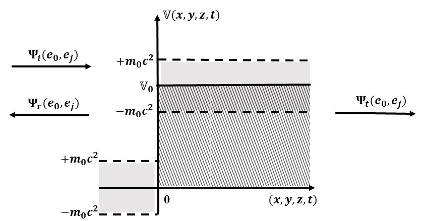
Figure 1: Schematic diagram of quaternionic step potential

A relativistic quaternionic Klein-Gordon equation for the step potential of regions $\mathbb{X}<0$ and $\mathbb{X}\geq 0$ shown in Fig. 1 takes form,

$$\left[-\frac{1}{c^{2}}\frac{\partial^{2}}{\partial t^{2}}+\nabla^{2}-\frac{m^{2}c^{2}}{\text{$\hbar$}^{2}}\right]\Psi(e_{0},e_{j})\,= \,\,0\,,\,\,\,\,\,\,\,\,\,\,(\mathbb{X}<0)\,,$$ (28)

$$\left[\left(\frac{i}{c}\frac{\partial}{\partial t}-\mathbb{V}_{0}\right)^{2}+\nabla^{2}-\frac{m^{2}c^{2}}{\text{\text{$\hbar$}}^{2}}\right]\Psi(e_{0},e_{j})\,= \,\,0\,,\,\,\,\,\,\,\,\,\,\,(\mathbb{X}\geq 0)\,\,.$$ (29)

The quaternionic wave function is now defined as

$$\Psi_{\text{$\mathbb{X}$$<0$}}\,\simeq \,\,\Psi_{\mathcal{I}}+\Psi_{\mathcal{R}}\,,\,\,\,\,\,\,\,\,\,\,(\mathbb{X}<0)$$ (30)

where $\Psi_{\mathcal{I}}$ is the quaternionic form of incident wave and $\Psi_{\mathcal{R}}$ is the quaternionic form of reflected wave, which can be further expressed as,

$$\Psi_{\mathcal{I}}(e_{0},e_{j})\,= \,\,\exp\left[-\frac{i}{\text{$\hbar$}}\left(Et-\boldsymbol{p}\cdot\boldsymbol{x}\right)\right]+\sum_{j=1}^{3}e_{j}\exp\left[-\frac{i}{\text{$\hbar$}}\left(-ict\boldsymbol{p}+\frac{iE}{c}\boldsymbol{x}-\left(\boldsymbol{p}\times\boldsymbol{x}\right)_{j}\right)\right]\,\,,$$ (31)

and

$$\Psi_{\mathcal{R}}(e_{0},e_{j})\,= \,\,\mathcal{R}\exp\left[-\frac{i}{\text{\text{$\hbar$}}}\left(Et+\boldsymbol{p}\cdot\boldsymbol{x}\right)\right]+\sum_{j=1}^{3}e_{j}\mathcal{R}\exp\left[-\frac{i}{\text{\text{$\hbar$}}}\left(-ict\boldsymbol{p}-\frac{iE}{\text{$c$}}\boldsymbol{x}+\left(\boldsymbol{p}\times\boldsymbol{x}\right)_{j}\right)\right]\,\,,$$ (32)

where $\mathcal{R}$ represents the amplitude for the reflected wave. As such, the quaternionic wave function for $\mathbb{X}\geq 0$ becomes $\Psi_{\text{$\mathbb{X}\geq 0$}}=\Psi_{\mathcal{T}}$, i.e.,

$$\Psi_{\mathcal{T}}(e_{0},e_{j})\,= \,\,\mathcal{T}\exp\left[-\frac{i}{\text{\text{$\hbar$}}}\left(Et-\boldsymbol{p}^{\prime}\cdot\boldsymbol{x}\right)\right]+\sum_{j=1}^{3}e_{j}\mathcal{T}\exp\left[-\frac{i}{\text{\text{$\hbar$}}}\left(-ict\boldsymbol{p}^{\prime}+\frac{iE}{\text{\text{$c$}}}\boldsymbol{x}-\left(\boldsymbol{p}^{\prime}\times\boldsymbol{x}\right)_{j}\right)\right],\,\,\,(\mathbb{X}\geq 0)\,,$$ (33)

with transmission amplitude $\mathcal{T}$ and momentum $\left|\boldsymbol{p^{\prime}}\right|=\,\sqrt{\frac{1}{c^{2}}\left(E-\mathbb{V}_{0}\right)^{2}-m_{0}^{2}c^{2}}$. Here, it is noticed that the kinetic energy of the transmitted particle will be lesser than that of the incident kinetic energy ($E$) because of the effect of step potential. Now, to solve the reflection and transmission coefficients for the relativistic step potential, we first calculate the reflected and transmitted amplitude of the quaternionic wave function by applying boundary conditions. Let us consider the boundary conditions

$$\left.\Psi_{\text{$\mathbb{X}$$<0$}}\right|_{\left(0,\,t\right)}\,= \,\,\left.\Psi_{\text{$\mathbb{X}\geq 0$}}\right|_{\left(0,\,t\right)}\,\,;$$ (34)

$$\left.\dot{\Psi}_{\text{$\mathbb{X}$$<0$}}\right|_{\left(0,\,t\right)}\,= \,\,\left.\dot{\Psi}_{\text{$\mathbb{X}\geq 0$}}\right|_{\left(0,\,t\right)}\,\,,$$ (35)

which gives

$$1+\mathcal{R} \,=\,\,\frac{\exp\left[-\frac{i}{\text{\text{$\hbar$}}}Et\right]+\sum_{j=1}^{3}e_{j}\exp\left[-\frac{ct}{\text{$\hbar$}}\boldsymbol{p}^{\prime}_{j}\right]}{\exp\left[-\frac{i}{\text{\text{$\hbar$}}}Et\right]+\sum_{j=1}^{3}e_{j}\exp\left[-\frac{ct}{\text{$\hbar$}}\boldsymbol{p}_{j}\right]}\mathcal{T}\,;$$ (36)

$$1-\mathcal{R} \,=\,\,\frac{\frac{i}{\text{\text{$\hbar$}}}\boldsymbol{p}^{\prime}\exp\left[-\frac{i}{\text{\text{$\hbar$}}}Et\right]+\sum_{j=1}^{3}\frac{E}{\text{\text{$\hbar$}}c}e_{j}\exp\left[-\frac{ct}{\text{\text{$\hbar$}}}\boldsymbol{p}^{\prime}_{j}\right]}{\frac{i}{\text{\text{$\hbar$}}}\boldsymbol{p}\exp\left[-\frac{i}{\text{\text{$\hbar$}}}Et\right]+\sum_{j=1}^{3}\frac{E}{\text{\text{$\hbar$}}c}e_{j}\exp\left[-\frac{ct}{\text{\text{$\hbar$}}}\boldsymbol{p}_{j}\right]}\mathcal{T}\,,$$ (37)

dividing (36) by (37), then simplifying, we get

$$|\mathcal{R}|^{2}\,= \mathcal{\,\,R}\mathcal{R}^{*}$$

$$= \,\frac{\left(\boldsymbol{p}-\boldsymbol{p}^{\prime}\right)^{2}+\left\{\boldsymbol{p}e^{\left[-\frac{ct}{\text{\text{$\hbar$}}}\boldsymbol{p}^{\prime}\right]}-\boldsymbol{p}^{\prime}e^{\left[-\frac{ct}{\text{\text{$\hbar$}}}\boldsymbol{p}\right]}\right\}^{2}+\frac{E^{2}}{c^{2}}\left\{e^{\left[-\frac{ct}{\text{\text{$\hbar$}}}\boldsymbol{p}^{\prime}\right]}-e^{\left[-\frac{ct}{\text{\text{$\hbar$}}}\boldsymbol{p}\right]}\right\}^{2}}{\left(\boldsymbol{p}+\boldsymbol{p}^{\prime}\right)^{2}+\frac{4E^{2}}{c^{2}}e^{\left[-\frac{2ct}{\text{\text{$\hbar$}}}\left(\boldsymbol{p}+\boldsymbol{p}^{\prime}\right)\right]}+\left\{\boldsymbol{p}e^{\left[-\frac{ct}{\text{\text{$\hbar$}}}\boldsymbol{p}^{\prime}\right]}+\boldsymbol{p}^{\prime}e^{\left[-\frac{ct}{\text{\text{$\hbar$}}}\boldsymbol{p}\right]}\right\}^{2}+\frac{E^{2}}{c^{2}}\left\{e^{\left[-\frac{ct}{\text{\text{$\hbar$}}}\boldsymbol{p}^{\prime}\right]}+e^{\left[-\frac{ct}{\text{\text{$\hbar$}}}\boldsymbol{p}\right]}\right\}^{2}}\,.$$ (38)

Here, $|\mathcal{R}|^{2}$ is the square of the amplitude of quaternionic reflected wave. Now, the quaternionic reflection coefficient (qRC) can be defined as

$$\mathbb{R}(e_{0},e_{j})=- \frac{J_{\mathcal{R}}}{J_{\mathcal{I}}}\,\,,$$ (39)

where $J_{\mathcal{R}}$and $J_{\mathcal{I}}$ are respectively the reflected and the incident probability current densities that can be determined by Eq.(26), such as

$$J_{\mathcal{R}}\,= \,\,\frac{\boldsymbol{p}}{m}|\mathcal{R}|^{2}+\frac{i\text{$\hbar$}}{2m}\sum_{j=1}^{3}e_{j}\left\llbracket\left(\frac{i\boldsymbol{p}}{\text{\text{$\hbar$}}}-\frac{E}{\text{\text{$\hbar$}}c}\right)\exp\left\{-\frac{i}{\text{\text{$\hbar$}}}\left[\left(Et+\boldsymbol{p}\cdot\boldsymbol{x}\right)-\left(ict\boldsymbol{p}+\frac{iE}{\text{\text{$c$}}}\boldsymbol{x}+\left(\boldsymbol{p}\times\boldsymbol{x}\right)_{j}\right)\right]\right\}\right.$$

$$\left.-\left(\frac{i\boldsymbol{p}}{\text{\text{$\hbar$}}}+\frac{E}{\text{\text{$\hbar$}}c}\right)\exp\left\{\frac{i}{\text{\text{$\hbar$}}}\left[\left(Et+\boldsymbol{p}\cdot\boldsymbol{x}\right)-\left(-ict\boldsymbol{p}-\frac{iE}{\text{\text{$c$}}}\boldsymbol{x}+\left(\boldsymbol{p}\times\boldsymbol{x}\right)_{j}\right)\right]\right\}\right\rrbracket|\mathcal{R}|^{2}\,\,,$$ (40)

and

$$J_{\mathcal{I}}\,= \,-\frac{\boldsymbol{p}}{m}+\frac{i\text{\text{$\hbar$}}}{2m}\sum_{j=1}^{3}e_{j}\left\llbracket\left(\frac{i\boldsymbol{p}}{\text{\text{$\hbar$}}}+\frac{E}{\text{\text{$\hbar$}}c}\right)\exp\left\{\frac{i}{\text{\text{$\hbar$}}}\left[\left(Et-\boldsymbol{p}\cdot\boldsymbol{x}\right)-\left(-ict\boldsymbol{p}+\frac{iE}{\text{$c$}}\boldsymbol{x}-\left(\boldsymbol{p}\times\boldsymbol{x}\right)_{j}\right)\right]\right\}\right.$$

$$\left.-\left(\frac{i\boldsymbol{p}}{\text{\text{$\hbar$}}}-\frac{E}{\text{\text{$\hbar$}}c}\right)\exp\left\{-\frac{i}{\text{\text{$\hbar$}}}\left[\left(Et-\boldsymbol{p}\cdot\boldsymbol{x}\right)-\left(ict\boldsymbol{p}-\frac{iE}{\text{$c$}}\boldsymbol{x}-\left(\boldsymbol{p}\times\boldsymbol{x}\right)_{j}\right)\right]\right\}\right\rrbracket\,\,,$$ (41)

Thus, from Eq.(39) the quaternionic reflection coefficient becomes

$$\mathbb{R}(e_{0},e_{j})\,=$$

$$-\frac{\frac{\boldsymbol{p}}{m}+\frac{i\text{\text{$\hbar$}}}{2m}\sum_{j=1}^{3}e_{j}\left[\left(\frac{i\boldsymbol{p}}{\text{\text{$\hbar$}}}-\frac{E}{\text{\text{$\hbar$}}c}\right)e^{-\frac{i}{\text{\text{$\hbar$}}}\left[Et+\boldsymbol{p}\cdot\boldsymbol{x}-ict\boldsymbol{p}-\frac{iE}{\text{\text{$c$}}}\boldsymbol{x}-\left(\boldsymbol{p}\times\boldsymbol{x}\right)_{j}\right]}-\left(\frac{i\boldsymbol{p}}{\text{\text{$\hbar$}}}+\frac{E}{\text{\text{$\hbar$}}c}\right)e^{\frac{i}{\text{\text{$\hbar$}}}\left[Et+\boldsymbol{p}\cdot\boldsymbol{x}+ict\boldsymbol{p}+\frac{iE}{\text{\text{$c$}}}\boldsymbol{x}-\left(\boldsymbol{p}\times\boldsymbol{x}\right)_{j}\right]}\right]}{-\frac{\boldsymbol{p}}{m}+\frac{i\text{\text{$\hbar$}}}{2m}\sum_{j=1}^{3}e_{j}\left[\left(\frac{i\boldsymbol{p}}{\text{\text{$\hbar$}}}+\frac{E}{\text{\text{$\hbar$}}c}\right)e^{\frac{i}{\text{\text{$\hbar$}}}\left[Et-\boldsymbol{p}\cdot\boldsymbol{x}+ict\boldsymbol{p}-\frac{iE}{\text{$c$}}\boldsymbol{x}+\left(\boldsymbol{p}\times\boldsymbol{x}\right)_{j}\right]}-\left(\frac{i\boldsymbol{p}}{\text{\text{$\hbar$}}}-\frac{E}{\text{\text{$\hbar$}}c}\right)e^{-\frac{i}{\text{\text{$\hbar$}}}\left[Et-\boldsymbol{p}\cdot\boldsymbol{x}-ict\boldsymbol{p}+\frac{iE}{\text{$c$}}\boldsymbol{x}+\left(\boldsymbol{p}\times\boldsymbol{x}\right)_{j}\right]}\right]}|\mathcal{R}|^{2}\,,$$ (42)

We can split the quaternionic reflection coefficient into two parts, where the pure scalar part yields

$$\mathbb{R}(e_{0},0) \,\,=\,|\mathcal{R}|^{2}\,,$$ (43)

while the pure quaternionic part becomes

$$\mathbb{R}(0,e_{j})\, =\,\,\sum_{j=1}^{3}e_{j}\left(\frac{\frac{E}{c}\cos\alpha-\boldsymbol{p}\sin\alpha}{\frac{E}{c}\cos\beta-\boldsymbol{p}\sin\beta}\right)\exp\left[-\frac{2E}{\text{$\hbar$}c}\boldsymbol{x}_{j}\right]|\mathcal{R}|^{2}\,,$$ (44)

where the parameters $\alpha=\frac{1}{\text{$\hbar$}}\left[Et+\boldsymbol{p}\cdot\boldsymbol{x}-\left(\boldsymbol{p}\times\boldsymbol{x}\right)\right]$ and $\beta=\frac{1}{\text{$\hbar$}}\left[Et-\boldsymbol{p}\cdot\boldsymbol{x}+\left(\boldsymbol{p}\times\boldsymbol{x}\right)\right]$. Therefore, it is conclude that the real quaternionic reflection coefficient has conventional meaning, however, the pure quaternionic reflection coefficient shows the additional part associated with quaternionic phase part and the decaying factor $\Omega(\boldsymbol{x}_{j})\,\sim\,\exp\left[-\frac{2E}{\text{$\hbar$}c}\boldsymbol{x}_{j}\right]$ along with $e_{j}-$ frames arise from the quaternionic wave function.
Besides, the quaternionic transmission coefficient (qTC) can be identified as

$$\mathbb{T}(e_{0},e_{j})\,= \,\,\frac{J_{\mathcal{T}}}{J_{\mathcal{I}}}\,\,,$$ (45)

where

$$J_{\mathcal{T}}\,= \,-\frac{\boldsymbol{p}^{\prime}}{m}|\mathcal{T}|^{2}+\frac{i\text{\text{$\hbar$}}}{2m}\sum_{j=1}^{3}e_{j}\left\llbracket\left(\frac{i\boldsymbol{p}^{\prime}}{\text{\text{$\hbar$}}}+\frac{E}{\text{\text{$\hbar$}}c}\right)\exp\frac{i}{\text{\text{$\hbar$}}}\left[\left(Et-\boldsymbol{p}^{\prime}\cdot\boldsymbol{x}\right)-\left(-ict\boldsymbol{p}^{\prime}+\frac{iE}{\text{$c$}}\boldsymbol{x}-\left(\boldsymbol{p}^{\prime}\times\boldsymbol{x}\right)_{j}\right)\right]\right.$$

$$\left.-\left(\frac{i}{\text{\text{$\hbar$}}}\boldsymbol{p}^{\prime}-\frac{E}{\text{\text{$\hbar$}}c}\right)\exp\left\{-\frac{i}{\text{\text{$\hbar$}}}\left[\left(Et-\boldsymbol{p}^{\prime}\cdot\boldsymbol{x}\right)-\left(ict\boldsymbol{p}^{\prime}-\frac{iE}{\text{$c$}}\boldsymbol{x}-\left(\boldsymbol{p}^{\prime}\times\boldsymbol{x}\right)_{j}\right)\right]\right\}\right\rrbracket\,|\mathcal{T}|^{2}\,\,.$$ (46)

Therefore, by substituting the value of $J_{\mathcal{T}}$ and $J_{\mathcal{I}},$ the quaternionic transmission coefficient becomes

$$\mathbb{T}(e_{0},e_{j})\,=$$

$$\frac{-\frac{\boldsymbol{p}^{\prime}}{m}+\frac{i\text{\text{$\hbar$}}}{2m}\sum_{j=1}^{3}e_{j}\left[\left(\frac{i\boldsymbol{p}^{\prime}}{\text{\text{$\hbar$}}}+\frac{E}{\text{\text{$\hbar$}}c}\right)e^{\frac{i}{\text{\text{$\hbar$}}}\left[Et-\boldsymbol{p}^{\prime}\cdot\boldsymbol{x}+ict\boldsymbol{p}^{\prime}-\frac{iE}{\text{$c$}}\boldsymbol{x}+\left(\boldsymbol{p}^{\prime}\times\boldsymbol{x}\right)_{j}\right]}-\left(\frac{i\boldsymbol{p}^{\prime}}{\text{\text{$\hbar$}}}-\frac{E}{\text{\text{$\hbar$}}c}\right)e^{-\frac{i}{\text{\text{$\hbar$}}}\left[Et-\boldsymbol{p}^{\prime}\cdot\boldsymbol{x}-ict\boldsymbol{p}^{\prime}+\frac{iE}{\text{$c$}}\boldsymbol{x}+\left(\boldsymbol{p}^{\prime}\times\boldsymbol{x}\right)_{j}\right]}\right]}{-\frac{\boldsymbol{p}}{m}+\frac{i\text{\text{$\hbar$}}}{2m}\sum_{j=1}^{3}e_{j}\left[\left(\frac{i\boldsymbol{p}}{\text{\text{$\hbar$}}}+\frac{E}{\text{\text{$\hbar$}}c}\right)e^{\frac{i}{\text{\text{$\hbar$}}}\left[Et-\boldsymbol{p}\cdot\boldsymbol{x}+ict\boldsymbol{p}-\frac{iE}{\text{$c$}}\boldsymbol{x}+\left(\boldsymbol{p}\times\boldsymbol{x}\right)_{j}\right]}-\left(\frac{i\boldsymbol{p}}{\text{\text{$\hbar$}}}-\frac{E}{\text{\text{$\hbar$}}c}\right)e^{-\frac{i}{\text{\text{$\hbar$}}}\left[Et-\boldsymbol{p}\cdot\boldsymbol{x}-ict\boldsymbol{p}+\frac{iE}{\text{$c$}}\boldsymbol{x}+\left(\boldsymbol{p}\times\boldsymbol{x}\right)_{j}\right]}\right]}\,|\mathcal{T}|^{2}.$$ (47)

The real part of quaternionic transmission coefficient will be contributed as

$$\mathbb{T}(e_{0},0)\,= \,\,|\mathcal{T}|^{2}\,\,,$$ (48)

while the pure quaternionic part contributes

$$\mathbb{T}(0,e_{j})\,= \,\,\sum_{j=1}^{3}e_{j}\left(\frac{\frac{E}{c}\cos\alpha^{\prime}-\boldsymbol{p}^{\prime}\sin\alpha^{\prime}}{\frac{E}{c}\cos\beta^{\prime}-\boldsymbol{p}\sin\beta^{\prime}}\right)\exp\left[-ct\left(\boldsymbol{p}^{\prime}-\boldsymbol{p}\right)\right]\,|\mathcal{T}|^{2}\,\,,$$ (49)

where $\alpha^{\prime}\,=\,\frac{1}{\hbar}\left[Et-\boldsymbol{p^{\prime}}\cdot\boldsymbol{x}+\left(\boldsymbol{p}^{\prime}\times\boldsymbol{x}\right)_{j}\right]$ and $\beta^{\prime}\,=\,\frac{1}{\hbar}\left[Et-\boldsymbol{p}\cdot\boldsymbol{x}+\left(\boldsymbol{p}\times\boldsymbol{x}\right)_{j}\right]$. Here, the real quaternionic transmission coefficient has usual form, but the pure quaternionic transmission coefficient has an additional part associated with the decaying factor $\exp\left[-ct\left(\boldsymbol{p}^{\prime}-\boldsymbol{p}\right)\right]$ for $e_{j}-$ axes arise from the quaternionic wave function. Further, if particles are not to be created or destroyed at the boundary as in a real quaternions, it strongly follows $\mathbb{R}+\mathbb{T}=1$, but for pure quaternionic case, the relation violates due to relativistic destroy in quaternionic space. Now, to check the significance of the quaternionic formalism, in following subsections we will discuss some important cases for the incident kinetic energy of particle that compare to the quaternionic step potential.

6.1 $\boldsymbol{E>\mathbb{V}_{0}+m_{0}c^{2}}$ : The oscillatory-like zone

In this case the kinetic energy of particle is greater than the sum of the step-potential and rest mass energy, then the momentum of the particle for region $\mathbb{X}\geq 0$ will be positive, i.e., $\left.\boldsymbol{P}^{\prime}\right|_{\mathbb{X}\geq 0}=\boldsymbol{p}^{\prime}$. Here, we assume that the lowest feasible value of step potential becomes the rest mass energy of particle. In order to check the quaternionic significance with time varying expression, we restrict our solutions only for time slaps $t\rightarrow 0$ and $t\rightarrow\infty$.

• Case 1: $t\rightarrow 0$. For this case, the square of reflection and transmission amplitude become:

  $$|\mathcal{R}|^{2}\,= \,\,\frac{\left(p-p^{\prime}\right)^{2}}{\left(p+p^{\prime}\right)^{2}-4p_{0}^{2}}\,\,\,;\,\,\,\,\,\,|\mathcal{T}|^{2}\,=\,\,\frac{4pp^{\prime}-4p_{0}^{2}}{\left(p+p^{\prime}\right)^{2}-4p_{0}^{2}}\,.$$ (50)

  Thus, the pure quaternionic form of reflection and transmission coefficients can be expressed by

  $$\mathbb{R}(e_{0},0)\,= \,\,|\mathcal{R}|^{2}\,,\,\,\,\,\mathbb{R}(0,e_{j})\,=\,\left(\frac{\frac{E}{c}\cos\alpha_{0}-\boldsymbol{p}\sin\alpha_{0}}{\frac{E}{c}\cos\beta_{0}-\boldsymbol{p}\sin\beta_{0}}\right)\Omega(\boldsymbol{x}_{j})|\mathcal{R}|^{2}\,;$$ (51)

  $$\mathbb{T}(e_{0},0)\,= \,\,|\mathcal{T}|^{2}\,,\,\,\,\,\mathbb{T}(0,e_{j})\,=\,\left(\frac{\frac{E}{c}\cos\alpha_{0}^{\prime}-\boldsymbol{p}^{\prime}\sin\alpha_{0}^{\prime}}{\frac{E}{c}\cos\beta_{0}-\boldsymbol{p}\sin\beta_{0}}\right)|\mathcal{T}|^{2}\,,$$ (52)

  where $\alpha_{0}=\frac{1}{\text{$\hbar$}}\left[\boldsymbol{p}\cdot\boldsymbol{x}-\left(\boldsymbol{p}\times\boldsymbol{x}\right)_{j}\right]$, $\beta_{0}=\frac{1}{\hbar}\left[-\boldsymbol{p}\cdot\boldsymbol{x}+\left(\boldsymbol{p}\times\boldsymbol{x}\right)_{j}\right]$and $\alpha_{0}^{\prime}=\frac{1}{\hbar}\left[-\boldsymbol{p^{\prime}}\cdot\boldsymbol{x}+\left(\boldsymbol{p}^{\prime}\times\boldsymbol{x}\right)_{j}\right]$. The reflection and transmission probability of a particle at the boundary of a quaternionic step potential is prevalent in pure scalar axes; however, it has some significant consequences in pure quaternionic axes. Despite the fact that the kinetic energy of a relativistic particle is greater than the quaternionic step potential, the probability of some particles reflecting back has a declining exponential component, whereas transmission has an oscillatory form for pure quaternionic space.

• Case 2: $t\rightarrow\infty$. In this case, the step potential width of forth-space component is taken extremely large. Then, the quaternionic reflection and transmission coefficients become:

  $$\mathbb{R}(e_{0},0)\,= \,\,\frac{\left(p-p^{\prime}\right)^{2}}{\left(p+p^{\prime}\right)^{2}}\,\,;\,\,\,\,\,\mathbb{R}(0,e_{j})\,=\,\Omega(\boldsymbol{x}_{j})|\mathcal{R}|^{2}\,\,,$$ (53)

  $$\mathbb{T}(e_{0},0)\,= \,\,\mathbb{T}(0,e_{j})\,=\,0\,.$$ (54)

  It is interesting to note that in this case, the quaternionic usual reflection coefficient is all that exists, and there is no quaternionic transmission for the potential steps that result from the fourth space component expanding towards infinity. The particle may therefore act like a classical particle.

6.2 $\boldsymbol{\left(\mathbb{V}_{0}-m_{0}c^{2}\right)<E<\left(\mathbb{V}_{0}+m_{0}c^{2}\right)}$: The tunnelling-like zone

In this case, the kinetic energy of the particle varies within the quaternionic effective potential, i.e., from $\mathbb{V}_{0}-m_{0}c^{2}$ to $\mathbb{V}_{0}+m_{0}c^{2}$ (see Fig. 1). Then, for this energy band, one can have

$$\left.\boldsymbol{P^{\prime}}\right|_{\mathbb{X}\geq 0}\,=\,i\boldsymbol{p^{\prime}}$$ (55)

where $\boldsymbol{P}^{\prime}$ indicates the imaginary momentum of the particle for region $\mathbb{X}\geq 0$, so we can simply replace $i\boldsymbol{p^{\prime}}$ instead of $\boldsymbol{p}$^′.

• Case 1: $t\rightarrow 0$. For this case, the square of reflection amplitude and transmission amplitude modified as:

  $$|\mathcal{R}|^{2}\,= \,\,\frac{\left(p-ip^{\prime}\right)^{2}}{\left(p+ip^{\prime}\right)^{2}-4p_{0}^{2}}\,\,;\,\,\,\,\,\,\,\,|\mathcal{T}|^{2}\,=\,\frac{4ipp^{\prime}-4p_{0}^{2}}{\left(p+ip^{\prime}\right)^{2}-4p_{0}^{2}}\,\,,$$ (56)

  which gives

  $$\mathbb{R}(e_{0},0)\,= \,\,|\mathcal{R}|^{2}\,;\,\,\,\,\mathbb{R}(0,e_{j})\,=\,\,\left(\frac{\frac{E}{c}\cos\alpha_{0}-\boldsymbol{p}\sin\alpha_{0}}{\frac{E}{c}\cos\beta_{0}-\boldsymbol{p}\sin\beta_{0}}\right)\Omega(\boldsymbol{x}_{j})|\mathcal{R}|^{2}\,,$$ (57)

  $$\mathbb{T}(e_{0},0)\,= \,\,|\mathcal{T}|^{2}\,;\,\,\,\,\mathbb{T}(0,e_{j})\,=\,\,\left(\frac{\frac{E}{c}\cos\alpha_{0}^{\prime}-i\boldsymbol{p}^{\prime}\sin\alpha_{0}^{\prime}}{\frac{E}{c}\cos\beta_{0}-\boldsymbol{p}\sin\beta_{0}}\right)|\mathcal{T}|^{2}\,.$$ (58)

  However, for time $t\rightarrow\tau$ the pure quaternionic transmission coefficient varies as

  $$\left.\mathbb{T}(0,e_{j})\right|_{t\rightarrow\tau}\,=\,\,\mathbb{T}(0,e_{j})\, e^{-\xi\,\tau}\,,$$ (59)

  where $\xi=c\boldsymbol{p}^{\prime}-c\boldsymbol{p}$ indicates the change of relativistic kinetic energy of a moving particle from region $\mathbb{X}<0$ to $\mathbb{X}\geq 0$. As a result of Eq.(59), the transmission coefficient for a pure quaternionic framework decays exponentially with time. Thus, the probability of identifying particles in $\mathbb{X}>0$ within such a tunnelling-like zone can be estimated by the fourth-space component of pure quaternionic space.

• Case 2: $t\rightarrow\infty$. The reflection and transmission coefficients for the infinitely extended step potential width due to the quaternionic fourth-space component are

  $$\mathbb{R}(e_{0},0)\,= \,\,|\mathcal{R}|^{2}\,\,\equiv\,\,\frac{\left(p-ip^{\prime}\right)^{2}}{\left(p+ip^{\prime}\right)^{2}}\,\,\,;\,\,\,\,\,\mathbb{R}(0,e_{j})\,=\,\Omega(\boldsymbol{x}_{j})|\mathcal{R}|^{2}\,\,,$$ (60)

  $$\mathbb{T}(e_{0},0)\,= \,\,\mathbb{T}(0,e_{j})\,=\,0\,.$$ (61)

  Essentially, as shown in subsection 6.2, only the quaternionic usual reflection coefficient is present in this situation, and no quaternionic transmission takes place for any hypothetical steps that result in the fourth space component stretching towards infinity.

6.3 $\boldsymbol{E<\left(\mathbb{V}_{0}-m_{0}c^{2}\right)}$: The Klein-like zone

This zone is crucial because if the particle’s kinetic energy is significantly lower than the height of the tunnelling-like zone, inappropriate particle reflection will have appeared. In order to analyze the Klein paradox behavior of relativistic particles in a quaternionic frame, let us write the momentum of the particle for region $\mathbb{X}\geq 0$, which becomes negative as

$$\left.\boldsymbol{P}^{\prime}\right|_{\mathbb{X}\geq 0}=\,\,-\boldsymbol{p}^{\prime}\,\,.$$ (62)

To examine the probability of particles in the regions $\mathbb{X}<0$ and $\mathbb{X}\geq 0$, we can place this opposite momentum value in Eqs.(39) and (45) as the following manner:

• Case 1: $t\rightarrow 0$. In this instance, the square of the reflection and transmission amplitudes of the quaternionic wave is adjusted as follows:

  $$|\mathcal{R}|^{2}\,\,=\,\,\frac{\left(p+p^{\prime}\right)^{2}}{\left(p-p^{\prime}\right)^{2}-4p_{0}^{2}}\,\,;\,\,\,\,\,\,\,\,\,|\mathcal{T}|^{2}\,\,= \,\,\frac{-4\left(pp^{\prime}+p_{0}^{2}\right)}{\left(p-p^{\prime}\right)^{2}-4p_{0}^{2}}\,\,.$$ (63)

  Hence, the quaternionic reflection coefficients i.e., $\mathbb{R}(e_{0},0),\,$$\mathbb{R}(0,e_{j})$ become:

  $$\mathbb{R}(e_{0},0)\,= \,\,|\mathcal{R}|^{2}\,\,\,;\,\,\,\,\,\,\mathbb{R}(0,e_{j})\,=\,\,\left(\frac{\frac{E}{c}\cos\alpha_{0}-\boldsymbol{p}\sin\alpha_{0}}{\frac{E}{c}\cos\beta_{0}-\boldsymbol{p}\sin\beta_{0}}\right)\Omega(\boldsymbol{x}_{j})|\mathcal{R}|^{2}\,\,.$$ (64)

  Since we see that $|\mathcal{R}|^{2}>1$, it is clear that the reflection coefficient increases and exceeds value one in both pure scalar and pure quaternionic circumstances that is providing an incompatible outcome for the quaternionic Klein paradox. A reflection coefficient larger than one caused by opposite momentum due to the quaternionic quantum fluctuations implies more particles will reflect that fall on it. However, the transmission coefficient changes to:

  $$\mathbb{T}(e_{0},0)\,= \,\,|\mathcal{T}|^{2}\,\,\,;\,\,\,\,\,\,\mathbb{T}(0,e_{j})\,=\,\left[\frac{\frac{E}{c}\cos\alpha_{0}^{\prime}+\boldsymbol{p}^{\prime}\sin\alpha_{0}^{\prime}}{\frac{E}{c}\cos\beta_{0}-\boldsymbol{p}\sin\beta_{0}}\right]|\mathcal{T}|^{2}\,\,.$$ (65)

  The relevance of the quaternionic Klein paradox is provided by the fact that $|\mathcal{T}|^{2}<0$, which means that the quaternionic transmission coefficients are negative for both pure scalar and pure quaternionic conditions.

• Case 2: $t\rightarrow\infty$. For this situation, the reflection and the transmission coefficients are expressed by

  $$\mathbb{R}(e_{0},0)\,= \,\,|\mathcal{R}|^{2}\,\equiv\,\frac{\left(p+p^{\prime}\right)^{2}}{\left(p-p^{\prime}\right)^{2}}\,\,\,;\,\,\,\,\,\,\,\,\mathbb{R}(0,e_{j})\,=\,\Omega(\boldsymbol{x}_{j})|\mathcal{R}|^{2}\,\,,$$ (66)

  $$\mathbb{T}(e_{0},0)\,= \,\,\mathbb{T}(0,e_{j})=\,0\,.$$ (67)

  Therefore, the probability of finding the particles in the reflected case is still greater than one, as explained in case $t\rightarrow 0$, but it impacts zero for the quaternionic transmitted probability when we increase the fourth dimension of space in the potential step up to infinity.

Hence, it is claimed that by reducing the step potential width at a small scale, the fundamental Klein-Gordon wave equation in quaternionic ($3+1$)$-$fields may be extended to explain the dynamics of relativistic particles in finite potential barrier.

7 Conclusion

The proposed research examines the Klein-Gordon wave equation in the context of quaternionic step potential by employing the $(3+1)-$dimensional quaternionic wave function. The quaternionic generalization of the Klein-Gordon equation has been established for both scalar and vector fields. We reviewed the quaternionic continuity-like equation that connected probability density and probability current density for pure scalars, pure vectors, and their mixed fields. It is intriguing that the combined field results from the mutual interaction of the real and pure quaternionic fields. Furthermore, the amplitudes of the incident, reflected, and transmitted waves for the quaternionic four-potential step have been analyzed. It is emphasized that the pure scalar component of the quaternionic incident, reflected, and transmitted waves is analogous to conventional waves; however, the additional or pure vector component of these waves appears due to the presence of a quaternionic structure. Correspondingly, we found the reflection and transmission coefficients associated with the quaternionic four-potential step, which demonstrate the probability of the existence of waves (or particles) in different regions of the step potential problem. Surprisingly, the quaternionic value of the reflected and transmitted coefficients is determined by the particle’s four-momentum. Furthermore, we have addressed the quaternionic interpretation for the oscillatory, tunnelling, and Klein paradox instances in which the incoming wave-function interacts with the potential step via the quaternionic momentum of the particle. It has also been claimed that the physical conservation law $\mathbb{R}+\mathbb{T}=1$ does not hold for pure quaternionic fields owing to non-commutativity, although it holds for pure scalar fields. Subsequently, it has been decided that, in order to account for the possibility of the quaternionic Klein paradox, the particle momentum in the step potential region ($\mathbb{X}\geq 0$) must be opposite to that region ($\mathbb{X}<0$), which suggests that the kinetic energy of the incoming wave (or particle) becomes negative. For the quaternionic Klein paradox, the quaternionic reflection coefficient becomes solely higher than one and the quaternionic transmission coefficient becomes simply less than zero. As a result, the current quaternionic ($3+1$) formalism is sufficiently consistent to explain the relativistic quantum phenomena of the contemporary era.

References

• [1] W. R. Hamilton, “Elementary of Quaternions”, Vol. I & Vol. II, Chelsea Publishing, New York, (1969).
• [2] P. A. Bolokhov, “Quaternionic wave function”, Int. J. Mod. Phys. A, 34 (2019), 1950001.
• [3] D. Finkelstein, J. M. Jauch and D. Speiser, “Quaternionic representations of compact groups”, J. Math. Phys., 4 (1963), 136.
• [4] S. L. Adler, “Quaternionic Quantum Mechanics and Quantum Fields”, Oxford University Press, (1995).
• [5] R. P. Feynman, “Space-time approach to non-relativistic quantum mechanics”, Rev. Mod. Phys., 20 (1948), 367.
• [6] A. Das, S. Okubo and S. A. Pernice, “Higher-dimensional SUSY quantum mechanics”, Mod. Phys. Lett. A, 12 (1997), 581.
• [7] L. Silberstein, “Quaternionic form of Relativity”, Philos. Mag., 23 (1912), 790.
• [8] S. Giardino, “Non-anti-Hermitian Quaternionic Quantum Mechanics”, Adv. Appl. Clifford Algebras, 28 (2018), 19.
• [9] S. Giardino, “Virial theorem and generalized momentum in quaternionic quantum mechanics”, Eur. Phys. J. Plus, 135 (2020), 114.
• [10] S. Giardino, “Quaternionic quantum mechanics in real hilbert space”, J. Geom. Phys. 158 (2020), 103956.
• [11] S. Giardino, “Quaternionic Klein–Gordon equation”, Eur. Phys. J. Plus, 136 (2021), 612.
• [12] S. Rawat, “Quaternionic Klein-Gordon equation in the electromagnetic field”, Eur. Phys. J. Plus, 137 (2022), 620.
• [13] A. J. Davies, “Quaternionic Dirac equation”, Phys. Rev., 41 (1990), 2628.
• [14] S. D. Leo and P. Rotelli, “The Quaternionic Dirac Lagrangian”, Mod. Phys. Lett. A, 11 (1996), 357.
• [15] M. Carmeli, “Field theory on R×S3 topology 1: The Klein-Gordon and Schrodinger equations”, Found. Phys., 15 (1983), 175
• [16] L. Silberstein, “Quaternionic form of Relativity”, Philos. Mag., 23 (1912), 790.
• [17] S. De Leo, “Quaternions and special relativity”, J. Math. Phys., 37 (1996), 2955.
• [18] W. Sprossig, “Quaternionic operator methods in fluid dynamics”, Adv. Appl. Clifford Algebras, 18 (2008), 963.
• [19] L. P. Horwitz and L. C. Biedenharn, “Quaternion quantum mechanics: second quantization and gauge fields”, Ann. Phys., 157 (1984) 432
• [20] S. De Leo, G. C. Ducati and C. C. Nishi, “Quateraionic potentials in non-relativistic quantum mechanics”, J. Phys. A: Math Gen., 35 (2002), 5411.
• [21] A. J. Davies and B. H. J. McKellar, “Nonrelativistic quaternionic quantum mechanics in one dimension”, Phys. Rev. A, 40 (1989), 4209.
• [22] S. Rawat and O. P. S. Negi, “Quaternion dirac equation and supersymmetry”. Int. J. Theor. Phys., 48 (2009), 2222.
• [23] S. Ulrych, “Higher spin quternion waves in the Klein Gordon Theory”, Int. J. Theor. Phys. 52 (2013), 279.
• [24] B. C. Chanyal, “A relativistic quantum theory of dyons wave propagation”, Can. J. Phys., 95 (2017), 1200.
• [25] B. C. Chanyal, “A new development in quantum field equations of dyons”, Can. J. Phys., 96 (2018), 1192.
• [26] B. C. Chanyal, “Quaternionic approach on the Dirac–Maxwell, Bernoulli and Navier–Stokes equations for dyonic fluid plasma”, Int. J. Modern Phys. A, 34 (2019), 1950202.
• [27] B. C. Chanyal, M. Pathak, “Quaternionic approach to dual Magneto-hydrodynamics of dyonic cold plasma”, Adv. High Energy Phys. 2018 (2018) Article ID 7843730, 13.
• [28] B. C. Chanyal, “On the quaternion transformation and field equations in curved space-time”, Proc. Natl. Acad. Sci., India, Sect. A Phys. Sci. 93 (2023), 185.
• [29] S. De Leo and S. Giardino, “Dirac solutions for quaternionic potentials”, J. Math. Phys., 55 (2014), 022301.
• [30] S. De Leo, G. Ducati and S. Giardino, “Quaternionic dirac scattering”, J. Phys. Math., 6 (2015),1 000130.
• [31] S. De Leo and G. Ducati, “Quaternionic differential operators”, J. Math. Phys., 42 (2001), 2236.
• [32] O. Klein, “The reflection of electron by a potential jump according to Dirac’s relativistic dynamics”, Zeit. Phys., 53 (1929), 157.
• [33] A. Calogeracos and N. Dombey, “History and physics of the Klein paradox”, Contemp. Phys., 40 (1999), 313.
• [34] H. Y. Wang, “Solving Klein’s paradox”, J. Phys. Commun., 4 (2020), 1.
• [35] A. Hansen and F. Ravndal, “Klein’s paradox and its resolution”, Phys. Scr., 23 (1981), 1036.
• [36] B. C. Chanyal and S. Karnatak, A comparative study of quaternionic rotational Dirac equation and its interpretation, Int. J. Geom. Methods Mod. Phys., 17 (2020) 2050018.
• [37] S. Bhatt and B. C. Chanyal, Generalized quaternionic free rotational Dirac equation and spinor solutions in the electromagnetic field, Int. J. Geom. Methods Mod. Phys., 19 (2022) 2250103.