Fast design and scaling of multi-qubit gates in large-scale trapped-ion quantum computers

Abstract

Quantum computers based on crystals of electrically trapped ions are a prominent technology for quantum computation. A unique feature of trapped ions is their long-range Coulomb interactions, which come about as an ability to naturally realize large-scale multi-qubit entanglement gates. However, scaling up the number of qubits in these systems, while retaining high-fidelity and high-speed operations is challenging. Specifically, designing multi-qubit entanglement gates in long ion crystals of 100s of ions involves an NP-hard optimization problem, rendering scaling up the number of qubits a conceptual challenge as well. Here we introduce a method that vastly reduces the computational challenge, effectively allowing for a polynomial-time design of fast and programmable entanglement gates, acting on the entire ion crystal. We use this method to investigate the utility, scaling and requirements of such multi-qubit gates. Our method delineates a path towards scaling up quantum computers based on ion-crystals with 100s of qubits.

I Introduction

Trapped ion quantum computers are a leading quantum computation platform, owing its success to the accurate control of individual ions, long-range connectivity and long coherence times. Despite their all-to-all connectivity, linear ion crystals of growing length present increasing difficulty in implementing high-fidelity and high-speed entanglement gates. Some trapped-ion scale-up architectures circumvent this challenge by interconnecting separate ion crystals, either by ion shuttling between segments in a quantum charge coupled device (QCCD) architecture [1, 2, 3] or by photonic interconnects [4, 5, 6]. However, both these approaches to scalability will benefit from working with longer ion crystals as their basic building block, by taking full advantage of the inherent long-range connectivity of the ions and its expected benefits [7, 8, 9, 10, 11].

Quantum information processing devices, based on crystals of 10s to 100s of trapped ions, have recently been implemented [12, 13, 14], overcoming hurdles such as crystal stability, cooling and coherence. Nevertheless, a prominent challenge which remains unaddressed is the design of multi-qubit entangling gates that are not hindered by the overwhelming spectral density of the normal modes of motion in large ion crystals. Specifically, designing the required control signals that generate high-fidelity, programmable, fast and robust multi-qubit entangling gates is a quadratically constrained NP-hard optimization problem [7], making the study of feasibility and scaling of large ion crystals a formidable challenge.

Here we introduce a method, coined large-scale fast (LSF), which efficiently designs multi-qubit entangling gates for large-scale ion crystals, enabling scaling up the trapped ion quantum processors to 100s of qubits in a single crystal. We show that a solution of a special instance of the optimization problem can be efficiently converted, using a linear transformation and local optimisations, to any other required entangling operation on the same system. Thus we find suitable approximate solutions in polynomial time. We use the LSF method to efficiently generate programmable multi-qubit $XX$-type entanglement operators and accumulate performance statistics of various coupling geometries such as all-to-all interactions, surface code stabilizer measurements, parallel pairwise gates, among other examples. We highlight that programmable $XX$ entangling gates, also known as ’Ising’ or ’global tunable’ gates, have been shown to be advantageous for improving the performance of quantum error correction codes [9], as well as for compilation of quantum Fourier transforms [8], Clifford unitary operators with a gate count that is independent of the qubit register size and $N$-qubit Toffoli gates [10].

We further show that while a crystal of $N$ ions can have $\mathcal{O}\left(N^{2}\right)$ types of different two-qubit gate interactions, naively resulting in a problem with dimension $N^{2}$, it is in fact sufficient to only solve $N$ quadratic constraints in order to find solutions to any required $XX$ gate. This enables efficient study of the scaling of various properties, such as gate time, fidelity and required power, with ion-crystals of 100’s of ions.

The LSF method has enabled us to study many types of couplings in large ion crystals and investigate their performance. This has generated a better understanding of the application of the entanglement operations, namely their advantages, limits and required resources. We show that the minimal entanglement time is determined by the smallest difference between the frequency of motional modes which are used in the gate, $\Delta\nu_{<}$. That is, $T_{\text{min}}=2\pi\Delta\nu_{<}^{-1}$. This scaling is intuitive as it corresponds to the time it takes the slowest phonon wave-packets to traverse the entire ion crystal. For transverse modes of $N$ equally-spaced ions this implies that $T_{\text{min}}\propto N^{2}$. Below that time scale, the solution we find requires a divergent power, and does not reach high gate fidelity.

Our analysis also presents an estimate of the power that is required in order to drive different gates. Specifically, we show that the power required to drive an arbitrary multi-ion entanglement operation can be predicted by extrapolating, from the power required for driving the entanglement operation in the adiabatic regime, on a different ion-crystal system in which this operation can be performed with global driving beams [7]. That is, many system details, such as ion participation in the modes of motion, or ion-qubit mapping, do not substantially affect the required power. This is quantified by a nuclear norm estimate, $\Omega_{\text{nuc}}$, of the coupling matrix $\varphi_{n,m}$, that determines the entangling phase between ions $n$ and $m$, i.e. the sum of its eigenvalues in absolute value, detailed below.

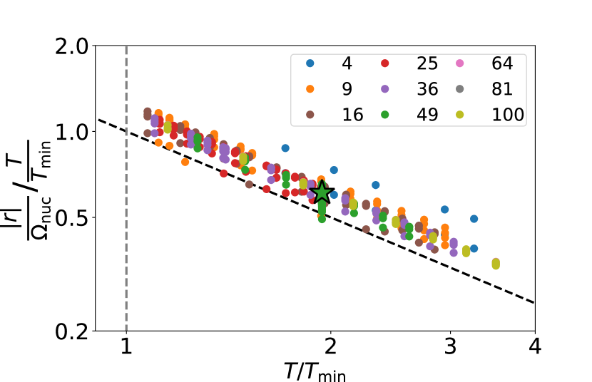
Figure 1: Summary of results obtained by our method, shown as total required Rabi frequency vs. gate time for various lengths of ion crystals (color), including a $N=100$ ion crystal. Each point corresponds to a different entanglement operation. The gate time (horizontal) is normalized by the minimal gate time, $T_{\text{min}}$ (vertical gray dashed line), and the total Rabi frequency, $\left|r\right|$, (vertical, log scale) is normalized according to the nuclear-norm based estimation, $\Omega_{\text{nuc}}$ and $T/T_{\text{min}}$, described below. As seen with this scaling, all our solutions collapse on a single line (black dashed), signifying an inverse proportion between required power and gate time. A specific realization (green star), of a single gate stabilizer measurement for a $N=49$ qubit surface code is analyzed in more detail below.

Figure 1 exhibits these results showing the total Rabi frequency required to drive entanglement gates, which vary in number of ions in the ion-crystal (color) and the types of gates used, as a function of the entanglement time. Each point in the plot corresponds to a specific crystal size and desired entanglement operation, and shows the gate performance averaged over 50 to 150 different solutions. We highlight that LSF enables a straightforward design of multi-qubit entangling gates over a $N=100$ qubit register. Both axes are scaled appropriately, such that all the data collapses approximately on the same unity slope line, showing we are able to generate correct estimates for the required gate power, as well as the minimal time for which our method is effective.

Figure 1 also highlights a specific realization (green star) which implements the entanglement gate necessary in order to perform a parallel stabilizer measurement of all relevant qubits, for a $N=49$ quantum error correction surface code. This realization is analyzed with further details below.

Lastly, while the character of the normal-modes of motion of trapped ion crystals is global, i.e. in general all ions participate in all modes, we show that the application of our method results in a reduction of the motion of ions which are not used in the operation. This is in stark contrast to the conventional method of entangling ions using a center-of-mass mode of motion, in which ions which are not driven and remain decoupled from the gate, are nevertheless displaced by the same amount as ions which are driven and coupled.

The remainder of the paper is ordered as follows, we first describe the derivation of the LSF method, then we perform an analysis of the total required Rabi frequency and derive the nuclear norm based estimate. Lastly, we focus on a specific realization (green star in Fig. 1) in order to highlight certain aspects of its operation.

II Derivation of the Large-scale fast method

Trapped ion quantum computers use the normal-modes of motion of the ion crystal as a phonon bus, which mediates interactions between the ion qubits. This is performed by driving the motional sidebands of the ion crystal, which generates spin-dependent forces. A canonical example of this method is the Mølmer-Sørensen (MS) gate [15, 16]. In recent years there have been many proposals and demonstrations which were focused on improving the utility and fidelity of MS gates. These methods are, at large, based on modulating spin-dependent displacement forces. This modulation may be implemented with various methods such as amplitude [8, 17], frequency [18] or phase modulation [19, 20] of the fields driving the ions. Using the LSF method we analyze the problem in the spectral domain [21, 22, 23]. That is, we fix a discrete set of frequency components of the radiation field driving the ions, and choose the (complex) amplitudes at each of these components according to the desired entangling operation. Since all other modulations can be decomposed in a Fourier series, the spectral representation is equivalent to an analysis in the time domain. Our method is therefore general.

The spectral approach taken here does offer conceptual advantages as it is easier to manipulate analytically [24] and offers physical intuition. Our approach is relevant to any form of qubit encoding; e.g. ground state, optical or metastable qubits [25], qubit drive; e.g. Raman, optical or laser-free, and architecture; e.g. global beam [26, 27] or individually controlled ions.

To generate a high-fidelity entangling gate, a qubit state which is initially unentangled with the motional degrees of freedom must remain so after the gate is performed. This requirement turns out to be linear in the drive amplitudes, and is relatively easy to satisfy. Additional linear constraints may be added in order to make the entanglement operation robust to various sources of error and noise (see Appendix A). In favor of a simple presentation, in what follows we assume that our degrees of freedom are written in a form that by-construction satisfies these constraints (see Appendix B).

Since the effective qubit-qubit interaction is quadratic in the driving field’s amplitude [7], generating a desired entangling operation reduces to the NP-hard quadratic optimization problem,

$$\text{argmin }\left|\bm{r}\right|\text{ such that }\bm{r}^{T}A_{n}\bm{r}=\varphi_{n}\quad\forall n=1,..,\mathcal{N}.$$ (1)

with $\left|\bm{r}\right|$ the norm of $\bm{r}\in\mathbb{R}^{\mathcal{M}}$, a vector representing $\mathcal{M}$ amplitudes, satisfying $\mathcal{N}$ quadratic constraints, with $\left\{A_{n}\in\mathbb{R}^{\mathcal{M}\times\mathcal{M}}\right\}_{n=1}^{\mathcal{N}}$ a set of real symmetric matrices, determined by the system parameters and $\left\{\varphi_{n}\right\}_{n=1}^{\mathcal{N}}$ a set of phases which encode the desired entangling operation. Simply put, we are seeking for the lowest power realization of the entangling operation.

The LSF method is general, such that the choice of system architecture determines the specific interpretation of $\bm{r}$ and the $A_{n}$’s. For example, we might use the setup considered in Ref. [7], which generates entangling gates for $N$ ions using a global beam. Here however we will focus on a more general setup, namely we consider $N$ ions which are individually addressed by $N$ independent driving fields, each having its own spectral content. We assume, without loss of generality, that all these spectra contain the same tones yet differ by the amplitudes of these tones (which could be null). This architecture enables qubit-qubit interactions which are mediated through the normal modes of motion and implements programmable $XX$ entangling gates, i.e unitary operators of the form, $U=\exp\left(i\sum_{n,m}\varphi_{n,m}\sigma^{\left(n\right)}_{x}\sigma^{\left(m\right)}_{x}\right)$, with $\sigma^{\left(n\right)}_{x}$ the Pauli-x operator acting on the $n$th qubit and $\varphi_{n,m}$ the ’target’ matrix, completely controllable. Accordingly this yields $\mathcal{N}=\mathcal{O}\left(N^{2}\right)$ quadratic constraints in direct correspondence to the target matrix, and $\bm{r}\in\mathbb{R}^{N\times M}$, with $M\propto N$, describing the distinct amplitudes of $M$ frequency pairs independently driving each of the $N$ ions.

We remark that the relevant time-scale for the gate-time is given by $\Delta\nu_{<}$, defined as the smallest difference between adjacent motional mode frequencies, which are used for the entanglement operation. Indeed in the adiabatic limit, i.e. for a gate time, $T$, such that $\Delta\nu_{<}T\gg 1$, the set of coupling matrices, $\{A_{n}\}_{n=1}^{\mathcal{N}}$ become diagonal, such that satisfying the quadratic constraints is trivial (see Appendix C). However due to the crowding of the mode frequencies in large ion crystals this results in impractically slow gates. Indeed as $2\pi\Delta\nu_{<}T\rightarrow 1$ the tones of the driving field strongly interact with many modes and the coupling matrices are in general dense, making the optimization problem non-trivial.

Using LSF, the NP-hard problem becomes independent of the desired gate, i.e. independent of $\left\{\varphi_{n}\right\}_{n=1}^{\mathcal{N}}$. We first explain this intuitively. We assume a non-trivial and normalized ’zero-phase solution’ satisfying the constraints in Eq. (1) with the ’zero’ target $\varphi_{n}=0$ for all $n=1,...,\mathcal{N}$, and denote it by $\bm{z}$, with $\left|\bm{z}\right|=1$. This solution can be scaled by any real number, i.e. $\lambda\bm{z}$ still satisfies the zero target. For a large enough $\lambda$ a small deviation, $\bm{d}$, from the zero-phase solution, i.e. $\bm{r}=\lambda\bm{z}+\bm{d}$, generates arbitrarily large entanglement phases. Thus we linearize the quadratic constraints in the vicinity of $\lambda\bm{z}$ and solve a linear equation for $\bm{d}$ that satisfies the constraints for a general target, $\bm{\varphi}$. This allows us to ’convert’ the zero-phase solution to a ’full’ solution of any desired target. Crucially, the linear equation depends on $\bm{\varphi}$ but the linearization does not, allowing for a quick conversion from the zero-phase solution to any solution of a general target. Accordingly, the ansatz solution satisfies the quadratic constraints of the full problem, but is still not necessarily optimal, in terms of its amplitude. Thus further optimization is performed by an iterative gradient descent, obtained by linearizing the quadratic equations.

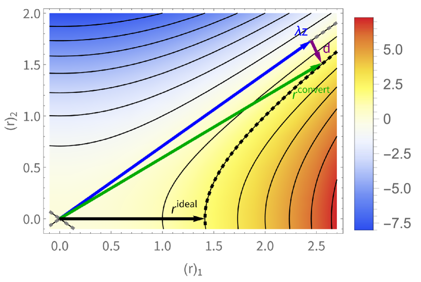
Figure 2: Simple example of the quadratically constrained optimization problem and our method. We choose $\mathcal{N}=1$, $\mathcal{M}=2$, specifically $A_{1}=\text{diag}\left(1,-2\right)$ and $\varphi_{1}=2$. The constraint becomes a hyperbola (black dashed) in terms of the two amplitudes, $r_{1}$ (horizontal axis) and $r_{2}$ (vertical axis), and the colored contours show other possible values of $\varphi$. The ideal solution is shown (black arrow). Our optimization method relies on the zero-phase solutions (gray dashed) and the high density of contours around $\lambda\bm{z}$, (blue arrow), such that only a small excursion by $\bm{d}$ (purple arrow) is required to convert $\bm{z}$ to a solution satisfying the constraints (green arrow). Here we have used $\lambda=3$.

Figure 2 shows this intuitive picture with a single quadratic constraint, i.e. $\mathcal{N}=1$, and two tones, i.e. $\mathcal{M}=2$. Specifically we use $A_{1}=\text{diag}\left(1,-2\right)$ and $\varphi_{1}=2$, such that the constraints are satisfied along a hyperbola (dashed black) in terms of the two amplitudes, $r_{1}$ (horizontal axis) and $r_{2}$ (vertical axis). Zero-phase solutions extend from the origin to arbitrarily large amplitudes (dashed gray). We use a large zero-phase solution, $\lambda\bm{z}$ (blue arrow), such that a small deviation from it, $\bm{d}$ (purple arrow), explores various values of $\varphi_{1}$. Indeed a converted solution, generating the desired target, $\varphi_{1}=2$, is found close by (green arrow). By linearization of the hyperbloid we perform gradient descent to gradually locate the locally ideal solution (black).

Specifically, we assume $\lambda$ is large, defined precisely below, and set $\bm{r}$, defined above, in the constraints of Eq. (1). We obtain,

$$\varphi_{n}=2\lambda\bm{z}^{T}A_{n}\bm{d}+\mathcal{O}\left(\epsilon\right),$$ (2)

with the assumption $\left|\bm{d}^{T}A_{n}\bm{d}\right|\leq\epsilon$, and $\epsilon$ the desired operation infidelity. The expression in Eq. (2) defines an easy linear equation, $\bm{\varphi}=M\bm{d}$, with $M_{n,k}=2\left(\bm{z}^{T}A_{n}\right)_{k}$, $n=1,...,\mathcal{N}$, and $k=1,...,\mathcal{M}$. It is solved by,

$$\bm{r^{\text{convert}}}=\lambda\bm{z}+\lambda^{-1}M_{\text{pinv}}^{-1}\bm{\varphi},$$ (3)

with $M_{\text{pinv}}^{-1}$ the pseudo-inverse of $M$. We set $\lambda$ such that our linearization is consistent, i.e.,

$$\left|\left(\frac{1}{\lambda}M_{\text{pinv}}^{-1}\bm{\varphi}\right)^{T}A_{j}\left(\frac{1}{\lambda}M_{\text{pinv}}^{-1}\bm{\varphi}\right)\right|\leq\epsilon.$$ (4)

The approximate solution in Eq. (3) satisfies the quadratic constraint, up to order $\epsilon$, but is still not optimal in terms of its magnitude. We iteratively improve it by a series of linear gradient descent steps that act to better satisfy the constraints and reduce the magnitude of the solution. This is done by defining the iteration, $\bm{r}^{\left(n\right)}=\bm{r}^{\text{optimal}}-\bm{d}^{\left(n+1\right)}$, with $\bm{r}^{\text{optimal}}$ the unknown local solution of the optimization problem and $\bm{r}^{\left(0\right)}=\bm{r^{\text{convert}}}$. At each step we calculate the constraint error, $\Delta\varphi^{\left(n+1\right)}_{j}=\varphi_{j}-\left(\bm{r}^{\left(n\right)}\right)^{T}A_{j}\bm{r}^{\left(n\right)}$. We then calculate the next correction by using,

$$\Delta\varphi_{j}^{\left(n+1\right)}=2\left(\bm{r}^{\left(n\right)}\right)^{T}A_{j}\bm{d}^{\left(n+1\right)}+\mathcal{O}\left(\epsilon\right).$$ (5)

As above the expression in Eq. (5) defines a linear relation which can be inverted and solved for the correction, $\bm{d}^{\left(n+1\right)}$. This will generate a solution which better satisfies the quadratic constraints. In order to also minimize its magnitude we use an additional linear condition, $\bm{r}^{\left(n\right)}\cdot\bm{d}^{\left(n+1\right)}=-\delta\left|\bm{r}^{\left(n\right)}\right|$, i.e. the correction $\bm{d}^{\left(n+1\right)}$ acts to reduce $\left|\bm{r}^{\left(n\right)}\right|$ by a small numerical step, $\delta$. All in all the linear iteration takes the form,

$$\begin{pmatrix}\Delta\bm{\varphi}^{\left(n\right)}\\ -\delta\left|\bm{r}^{\left(n\right)}\right|\end{pmatrix}=\begin{pmatrix}M^{\left(n\right)}\\ \bm{r}^{\left(n\right)}\end{pmatrix}\bm{d}^{\left(n+1\right)},$$ (6)

with $M^{\left(n\right)}_{j,k}=2\left(\left(\bm{r}^{\left(n\right)}\right)^{T}A_{j}\right)_{k}$. Finally we set $\bm{r}^{\left(n+1\right)}=\bm{r}^{\left(n\right)}+\bm{d}^{\left(n+1\right)}$.

These results imply a recipe for efficiently generating solutions of Eq. (1). Namely, we aggregate many distinct zero-phase solutions (see Appendix D). Then, given a desired target gate, represented by $\bm{\varphi}$, we obtain a solution, $\bm{r}$, by using Eq. (2) and the linear iteration in Eq. (6). This process can be done rapidly and in parallel for all of the aggregated zero-phase solutions, out of which the best performing solution is chosen.

Lastly, we note that aggregation of zero-phase solutions may be performed under the assumption of a global drive, i.e. that the spectrum of all of the ions is identical. This recovers the setup of Ref. [7] in which only $N$ quadratic constraints, associated with the phase accumulated by the $N$ modes of motion, are required to vanish. Nevertheless, these zero-phase solutions can then be readily converted to full solutions of independently driven ions, avoiding the need to ever solve a dimension $N^{2}$ quadratically constrained problem. Remarkably, the performance of our solutions that are converted from zero-phase solutions of an $N$-dimensional quadratic ansatz have a similar fidelity and power, compared to solutions that are converted from zero-phase solutions of an $N^{2}$-dimensional quadratic problem, representing the full degrees of freedom of the system (see Appendix G).

III Entanglement scalability in large ion crystals

We use LSF in order to investigate performance and scalability of entanglement operations in large ion crystals. To this end we consider many trapped ions systems which vary in number of ions, operations time, drive spectra, etc. For each such system we aggregate approximately 150 zero-phase solutions and convert them to full solutions of many entanglement targets, $\varphi_{n,m}$.

We first observe that we find many zero-phase solutions for systems for which $T>T_{\text{min}}=2\pi\Delta\nu_{<}^{-1}$ with $\Delta\nu_{<}^{-1}$ the smallest frequency difference of adjacent normal modes of motion. For ions coupled via transverse modes this yields $T_{\text{min}}\propto N^{2}$. The $N^{2}$ dependence originates from the divergence of density of states of phonon modes at the part of the motional spectrum in which $\nu\propto k^{2}$. This yields one factor of $N$ due to the density of states, and another factor of $N$ due to the crystal length.

Indeed, Fig. 1 shows solutions for various number of ions (color) and operation time (horizontal), scaled by $T_{\text{min}}$. For times $T<T_{\text{min}}$ we either do not find zero-phase solutions or find solutions with a seemingly diverging power and high infidelity of the converted full solutions. We note that this limit is determined by the ion crystal spectrum and is agnostic to the target unitary, i.e. entangling ions at the two edges of the crystal can be performed at the same minimal gate time as that of neighbouring ions. This stems from the fact that the modes of motion of the ion crystal are global, i.e. involve all ions in the crystal, and that in the fast-gate limit all of the modes are excited. The minimal gate time, of high-fidelity realizations, is therefore given by the time it takes the slowest sound mode to traverse the crystal.

We benchmark the solutions produced by LSF using a small scale, $N=4$, simulation. The simulation takes into account the evolution of the ions and the phonon modes under the model Hamiltonian (see Appendix A), as well as next-order corrections, such as off-resonance coupling to the qubit carrier transition and higher-order Lamb-Dicke terms. All of the simulated gates exhibit a high operation fidelity, matching the performance predicted by LSF (see Appendix E).

Next we consider the total Rabi frequency required to drive the entanglement gate, which we quantify as $\left|\bm{r}\right|\equiv\sqrt{\sum_{n,m}\left(\bm{r}_{n}\right)_{m}^{2}}$. Since the gate design stems from an NP-hard problem, one would expect that predicting the required total Rabi frequency, before solving the optimization problem, to be challenging. Nevertheless such a prediction is useful as it can be used for system design and as an a-priori stopping criteria for the gradient descent process.

We address this challenge by the following analysis. We first recall the expression for the Rabi frequency required to drive a MS gate, $\Omega_{\text{MS}}=\frac{\sqrt{\left|\varphi_{\text{MS}}\right|}}{\sqrt{2\pi}\eta T}$, with $\varphi_{\text{MS}}$ the entanglement phase, and $\eta\propto\nu^{-1}$ the Lamb-Dicke parameter corresponding to the mode of motion at frequency $\nu$. This expression is valid in the adiabatic limit, i.e. for $T\gg\nu^{-1},\Delta\nu_{<}^{-1}$. We then generalize $\Omega_{\text{MS}}$ to a system in which the target $\varphi_{n,m}$ is native, i.e. it can be implemented with a global driving field. This is achieved in the case where that the normal-modes of motion of the ion crystal are the eigenvectors of the matrix $\varphi_{n,m}$ [7], and each mode accumulates a phase that is the corresponding eigenvalue. We incorporate this change by replacing $\varphi_{\text{MS}}\mapsto\sum_{j=1}^{N}\left|\varphi_{j}\right|$ , with $\left\{\varphi_{j}\right\}$ the eigenvalues of $\varphi_{n,m}$. This sum is known as the ’nuclear norm’ of the matrix $\varphi_{n,m}$. Furthermore we replace $\eta$ with the average $\eta$ over all modes of motion. When we go beyond native targets, we replace all the elements of $\varphi_{n,m}$ with their absolute value. Lastly, for independently driven ions we expect the power to scale linearly with $N$. Thus, we conjecture an estimate, $\Omega_{\text{nuc}}$,

$$\Omega_{\text{nuc}}=k\frac{\sqrt{N\text{nuc}\left(\left|\varphi_{n,m}\right|\right)}}{\sqrt{2\pi}\langle\eta\rangle T},$$ (7)

with $\text{nuc}\left(\left|\cdot\right|\right)$ the nuclear norm of a matrix with its elements taken in absolute value, and $k$ a constant which depends on the choice of implemented linear constraints (e.g. additional linear constraints ensuring gate robustness).

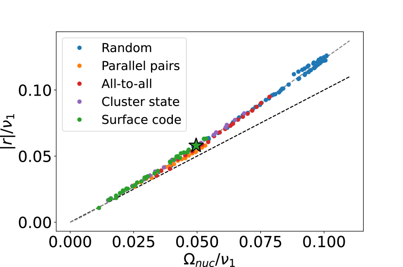
Figure 3: Benchmarking of the nuclear-norm estimation on a $N=49$ ion crystal. Estimation based on the nuclear norm (horizontal) is compared to our method’s solutions (vertical), for various entanglement gates. Each entanglement target is converted to full solutions using 150 zero-phase solutions. The average (point) Rabi frequency is shown. The entanglement operations are divided to different groups (all on the same ion crystal): randomly generated patterns (blue), parallel pairwise interactions (orange), all-to-all interactions of subsets of the crystal (red), arrangements of subsets of the ions in a grid to form cluster states (purple) and the entanglement operation required for a stabilizer measurement of a surface code, on subsets of the ions (green). With this scaling the various targets collapse on a line, which slightly deviates from our estimation (black dashed). We use numerical fit to slightly vary the exponent of the nuclear-norm from $0.5$ to $0.551$, yielding a good fit (gray dashed).

We benchmark this estimate on our set of solutions, and find that this naive estimate gives surprisingly accurate prediction of $\left|\bm{r}\right|$, with the proportionality constant in Eq. (7) fitted to $k=4$. Indeed, Fig. 3 shows various entanglement targets (points), on a $N=49$ ion crystal, which are separated to different conceptual groups: randomly generated patterns (blue), parallel pairwise interactions (orange), all-to-all interactions of subsets of the crystal (red), arrangements of subsets of the ions in a grid, to form a cluster state (purple) and the entanglement operation required for a stabilizer measurement of a surface code, on subsets of the ions (green).

All of these solutions are based on the same collection of zero-phase solutions, and implement the gate time at $T\approx 2T_{\text{min}}\approx 12.9\text{ms}$. For each of these solutions we show the average (point) total Rabi frequency obtained by the conversion of the many zero-phase solutions. We compare our nuclear-norm conjecture in Eq. (7) (horizontal) with LSF’s result (vertical), showing that all the solutions collapse on a line. Our conjecture predicts this collapse to occur on a line of unity slope (black dashed). However we observe that the actual results slightly deviate. We correct for this deviation by changing the square root of the nuclear norm, in Eq. (7), to an arbitrary exponent, which is numerically fitted to $0.551$ (gray dashed), and matches well with the data.

Remarkably, the data collapse shown in Fig. 3 implies that the details of the mode structure and frequency are largely irrelevant to the required Rabi frequency. The analogy to a globally driven system provides an intuitive explanation: Driving the ions independently is equivalent to an effective ’reshaping’ of the participation of each ion in each of the normal-modes, such that the resulting reshaped mode structure fits the required operation better. Here indeed, this reshaping causes the nuclear norm conjecture to match closely with the full computation, with a small overhead, that comes about as a modification of the exponent of the nuclear norm. We emphasize that while this picture is intuitive, it could not have been verified without the ability to compute optimal, multi-mode, entanglement gates on large ion crystals, afforded by LSF.

We remark that the conjectured estimation based on the nuclear norm assumes that the modes of motion of the ion crystal are global, i.e. that in general all ions are coupled to each other. Indeed in a pathological case in which all ions oscillate independently from one other, ion-ion entanglement is impossible, yet the nuclear norm estimate will not diverge. Furthermore, we note that other known matrix norms operating on $\varphi_{n,m}$, do not generate the data-collapse shown in Fig. 3 above.

IV Surface code stabilizer operation

We demonstrate our method and highlight certain aspects of it via an example. Specifically we outline the entanglement gate required for stabilizer measurements in surface codes. Here we consider a 49 ions crystal, entangling 33 ions using a single pulse. Figure 4 shows the formation of the stabilizer (left), namely by setting appropriate non-zero coupling phases (black arrows) we map the ion crystal (top) to a $7\times 7$ square grid (bottom), and form nine plaquettes (yellow) which can be used to evaluate the $X$-parity of the plaquette vertices. In this straightforward mapping some ions remain uncoupled (orange) and can be used in other subsequent operations, some form edge of plaquettes (blue) and some are designated as ancilla qubits (dark blue).

It was shown in Ref. [28] that a surface code stabilizer measurement can be implemented with a single multi-qubit MS gate. Note, however, that our coupling map between ions involved in a stabilizer measurement is not all-to-all; rather it takes the form of a ’cross’. This is in fact more efficient as it requires fewer non-zero entanglement phases. Indeed the nuclear norm of the cross coupling map is two times lower than that of the all-to-all coupling.

Figure 4: Multi-mode stabilizer measurement in the surface code implemented on a 49 ion equi-distant crystal. Left: Our method is used in order to generate a stabilizer measurement in a 49 ions crystal surface code (top). The 49 ions are used to form the surface code (bottom), namely nine plaquettes (yellow) for which the $X$-parity can be measured. In this scheme some ions are coupled (blue) by pairwise links (black arrows) and others are not (orange). Ions with four links, in the plaquette centers (dark blue) are ancilla qubits. Right: Solution statistics due to the conversion of 150 zero-phase solutions. All solutions generate similar performance in terms of the required drive power (vertical) and all meet the fidelity threshold, here set to $1-10^{-4}$ (horizontal). We highlight a specific realization (green star) which we further analyze and present below.

Here we assume an equally spaced crystal of ${}^{40}\text{Ca}^{+}$ ions with an inter-ion distance of $5\text{ }\mu\text{m}$. Qubits are mapped on the ground state Zeeman $5S_{\frac{1}{2}}$ manifold and are driven with a $400\text{nm}$ laser field using a Raman transition, which couples the ions using transverse modes of motion, at frequencies of $3\text{ MHz}$ to $3.5\text{ MHz}$. We choose an operation time $T\approx 2T_{\text{min}}\approx 12.9\text{ms}$. We use our method as prescribed above in order to generate the required entanglement gate. In order to effectively benchmark our method we aggregate 150 zero-phase solutions which are all converted to solutions of the full optimization problem and analyzed. Figure 4 (right) shows the expected infidelity (horizontal) and required total Rabi frequency (vertical) to drive these solutions, normalized to the frequency of the first mode of motion, at $3$ MHz. All solutions exhibit a low infidelity, defined as,

$$I=\sum_{n,m}\Delta\varphi_{n,m}^{2}=\sum_{n,m}\left(\varphi_{n,m}^{\text{ideal}}-\varphi_{n,m}^{\text{actual}}\right)^{2}.$$ (8)

This definition is an operational distance measure between the ideal entanglement phases, $\varphi_{n,m}^{\text{ideal}}$ and the phases achieved by our method, $\varphi_{n,m}^{\text{actual}}$. At the limit of small phase differences this definition converges to the actual operation’s infidelity [29].

For the sake of comparison, in this setup a conventional MS gate with the same gate time and coupled to the first motional mode, $\nu_{1}$, requires a total amplitude of approximately $0.108\nu_{1}$ and will have a low gate fidelity, due to operating outside of its adiabatic regime. In contrast, all of our solutions exhibit a similar total amplitude, yet feature a high fidelity, with few outliers. This implies that it is not necessary to aggregate many zero-phase solutions, as they are in general similar in performance. We highlight a low-power solution (green star) which is further analyzed below.

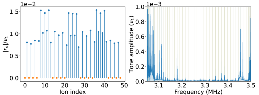
Figure 5: Spectral analysis of highlighted solution. Left: Drive amplitude per ion, $\left|\bm{r}_{n}\right|$. Our method converges to a solution for which the drive of uncoupled ions (orange) is shut off while coupled ions are driven (blue). We note that ions 8, 10, 12, 22, 24, 26, etc. are driven most strongly, as these ions have each four links, seen in Fig. 4. Right: Tone amplitudes (in absolute value) used to drive the highlighted gate, averaged over ions (blue), and their standard deviation (shaded). Clearly the spectrum is dominant in the vicinity of the lower modes of motion (olive) as these modes are of higher wave-number and are better suited for differentiating between the entanglement of adjacent ions.

We consider the spectrum given by the highlighted solution (green star in Fig. 4). Some of the ions are decoupled from the stabilizer measurement (orange in Fig. 4) and are not required to be illuminated or driven at all by a spin-dependent force. Indeed, Fig. 5 (left) shows the total power that is driving each ion, showing that the decoupled ions are not driven. We emphasize that our optimization was not constrained to provide such a solution, i.e. the conversion of the zero-phase solution and the subsequent gradient descent have automatically converged to shutting off the illumination of decoupled ions. Furthermore, we note that ancilla ions, i.e. ions 8, 10, 12, 22, 24, 26, etc. (dark blue in Fig. 4), which have more couplings to ions in the crystal, are accordingly driven with a stronger field.

Next we consider the average spectrum driving the ions, shown in Fig. 5 (right). The coupling pattern required for the surface code, when mapped to the linear crystal, requires significant variation between adjacent ions (e.g some links are nearest neighbours and some are long range), which are more efficiently formed with high wave-number modes of motion. Indeed the drive tones (blue) are clearly focused around these modes (olive), which for transverse normal-modes, reside at the low-frequency end of the spectrum. These modes also have a slightly larger Lamb-Dicke parameter, which quantifies the coupling between the drive and spin-dependent displacement, thus they better utilize the drive power, and practically a lower heating rate (although not considered in this analysis), resulting in a high-fidelity realization. Figure 5 (right) also shows that we only make use of driving tones which are close, compared to $T^{-1}$, to motional modes. We have seen that these tones are the main contributors to the gate solution, and thus enable a reduction in the number of degrees of freedom used in the optimization.

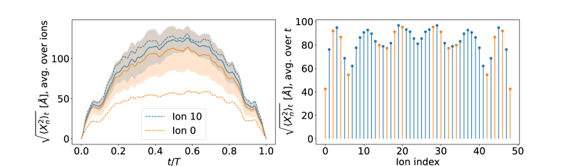
Figure 6: Ion motion. Left: Standard deviation of ion motion during the entanglement operation. Averaged on coupled ions (blue) including standard deviation (shaded), and on uncoupled ions (orange), which are also displaced by our drive. As shown above coupled ions are illuminated and therefor are more displaced than the uncoupled ions. We highlight ion number 10 (blue dashed), which is coupled to four ions and therefore moves significantly compared to uncoupled ions such as ion number 0 (orange dashed). Right: Standard deviation of ion motion, average on time. Here as well it is seen that ions that are driven exhibit, in general, a larger displacement than ions which are not driven, emphasizing the utility of the solutions provided by our method. The inversion-symmetry character of the modes of motion is apparent and manifests as a symmetry in the standard deviation of motion among ions.

Lastly we consider the ion-displacement, $X_{n}$, induced by the drive implemented on the ions. The ion-displacement is spin-dependent, i.e. its direction and magnitude depend on spin-projections along the Pauli-$x$ axis. Since the qubit ground state is composed of an equal superposition of all eigenstates along the Pauli-$x$ axis then, by symmetry, the mean displacement vanishes. However the time-dependent variance of the spin displacement, is non-vanishing, and is given by (see Appendix F),

$$\expectationvalue{X_{n}^{2}}_{t}=\sum_{j=1}^{N}\left(O_{j}^{\left(n\right)}\right)^{2}\expectationvalue{x_{j}^{2}}_{t},$$ (9)

with $\expectationvalue{x_{j}^{2}}_{t}$ the time-dependent variance of the displacement of mode $j$ and $O_{j}^{\left(n\right)}$ the normalized participation of ion $n$ in mode $j$ (see Appendix F).

Figure 6 (left) shows $\sqrt{\expectationvalue{X_{n}^{2}}_{t}}$, averaged over ions, with ions which are used in the stabilizer operation (blue) and ions which are uncoupled (orange), as a function of time. Since the modes of motion couple, in general, all ions in the crystal, then ions which are not illuminated still exhibit motion, however this motion is reduced compared to the ions which are illuminated. This highlights an apparent advantage of independently addressed ions, namely the spectra which drives each ion is effectively used to tune the participation of each ion in each mode of motion, generating an optimal realization of the operation. Furthermore we consider the variance, averaged over time (right), which reveals that uncoupled ions (orange) in general have a smaller displacement. Furthermore, the inversion-symmetry character of the modes of motion is apparent and manifests as a symmetry in the deviation, i.e. the motions of ion $n$ and $N-n$ are identical. This implies that an efficient mapping from the linear crystal to the implemented models can be used in order to minimize unnecessary motion.

In summary, we have introduced a method, large-scale fast, which helps mitigate some of the NP-hardness of designing large-scale entanglement gates for trapped ions qubits. Our method requires a few initial special solutions, solving $N$, and not $N^{2}$, quadratic constraints, which are then readily converted to entanglement gates of arbitrary programmable targets. This allows us to construct specific interactions, such as parallel stabilizer measurements for quantum error correction surface codes. Furthermore, we use our method in order to investigate various aspect of multi-qubit entanglement gates of large ion crystals. Our method delineates a path towards trapped ion crystals of 100s of ions and offers a resolution to the gate-design problem.

Appendix A: Model derivation

We detail the derivation of the model used to formulate the optimization problem in Eq. (1). In our analysis below we rely on and generalize the derivations provided in [7].

We consider a general spectrum of tones which drive independently $N$ trapped ions. Without loss of generality, the driving applied to different ions may be regarded as composed of the same tones, differing only by the tone amplitudes. These tones are placed symmetrically around the single qubit transition frequency, $\omega_{0}$. The field driving the $n$th ion is,

$$\begin{split}w_{n}\left(t\right)=&2\cos\left(\omega_{0}t+\phi_{0}\right)\\ \cdot&\sum_{m=1}^{M}\left[\left(\bm{r}_{n}^{\left(c\right)}\right)_{m}\cos\left(\omega_{m}t\right)+\left(\bm{r}_{n}^{\left(s\right)}\right)_{m}\sin\left(\omega_{m}t\right)\right].\end{split}$$ (10)

That is, each spectrum contains $2M$ components at frequencies $\left\{\omega_{0}\pm\omega_{m}\right\}_{m=1}^{M}$. The amplitude of the cosine (sine) $m$th tone pair illuminating the $n$th ions is $\left(\bm{r}_{n}^{\left(c\right)}\right)_{m}$ ($\left(\bm{r}_{n}^{\left(s\right)}\right)_{m}$) and the phase of each tone in the pair is $\phi_{0}\pm 0$ ($\phi_{0}\mp\pi/2$), such that all $N\times M$ tone pairs have the same average phase, which generates a correlated rotation around the Pauli $\sin\left(\phi_{0}\right)\sigma_{x}+\cos\left(\phi_{0}\right)\sigma_{y}$ axis. For simplicity we assume that $\phi_{0}=\pi/2$ such that the relevant Pauli operator is $\sigma_{x}$. The motional mode phase space trajectories generated by the cosine and sine quadrature are relatively rotated by $\pi/2$.

All in all this is captured by the lab-frame Hamiltonian ($\hbar=1$),

$$\begin{split}H&=H_{0}+V\\ H_{0}&=\sum_{j=1}^{N}\left[\nu_{j}\left(a^{\dagger}_{j}a_{j}+\frac{1}{2}\right)+\frac{\omega_{0}}{2}\sigma_{z}^{\left(j\right)}\right]\\ V&=2\Omega\sum_{n=1}^{N}\sigma_{x}^{\left(n\right)}\cos\left(kx_{n}-\omega_{0}t\right)\cdot\\ &\sum_{m=1}^{M}\left[\left(\bm{r}_{n}^{\left(c\right)}\right)_{m}\cos\left(\omega_{m}t\right)+\left(\bm{r}_{n}^{\left(s\right)}\right)_{m}\sin\left(\omega_{m}t\right)\right],\end{split}$$ (11)

with $a_{j}$ the annihilation operator associated with $j$th normal mode of motion, at frequency $\nu_{j}$, $\sigma_{i}^{\left(n\right)}$ the $i$-Pauli operator acting on the $n$th ion, $k$ the driving field’s wave number, $x_{n}$ the position operator of the $n$th ion and $\Omega$ a characteristic Rabi frequency. Clearly the last parenthesis in Eq. (11) can be written as a single cosine term with a phase, however this form preserves a crucial aspect of our formulations, i.e. the exclusive linear and quadratic dependence on the amplitudes. Furthermore, here we have assumed that we are coupled to motional modes along one principle direction of the trap, such that the summation on modes is up to $N$ (and not $3N$), this assumption can be easily relaxed [30].

By using a conventional set of approximations, namely the rotating wave approximation in $\Omega/\omega_{0}$, the Lamb-Dicke approximation, and by neglecting carrier-coupling terms the lab-frame Hamiltonian is converted to the interaction Hamiltonian,

$$\begin{split}H_{\text{I}}&=\Omega\sum_{n=1}^{N}\sigma_{x}^{\left(n\right)}\sum_{j=1}^{N}\eta_{j}O_{j}^{\left(n\right)}\left(a_{j}^{\dagger}e^{i\nu_{j}t}+\text{H.c}\right)\cdot\\ &\sum_{m=1}^{M}\left(\left(\bm{r}_{n}^{\left(c\right)}\right)_{m}\cos\left(\omega_{m}t\right)+\left(\bm{r}_{n}^{\left(s\right)}\right)_{m}\sin\left(\omega_{m}t\right)\right),\end{split}$$ (12)

with $O_{j}^{\left(n\right)}$ the normalized participation of the $n$th ion in the $j$th mode of motion, such that $\sum_{j=1}^{N}O_{n}^{\left(j\right)}O_{m}^{\left(j\right)}=\delta_{n,m}$, and $\eta_{j}$ the singe-ion Lamb-Dicke parameter associated with the $j$th mode of motion (it is sometimes conventional to define $\eta_{j}^{\left(n\right)}=\eta_{j}O_{j}^{\left(n\right)}$).

The Hamiltonian in Eq. (12) can be rearranged in the form, $H_{\text{I}}=\sum_{n=1}^{N}\sum_{j=1}^{N}\zeta_{j}^{\left(n\right)}\left(t\right)\sigma_{x}^{\left(n\right)}a_{j}+\text{H.c}$, with $\zeta\left(t\right)$ a time dependent function read-off directly from Eq. (12). That is, it has only $\sigma_{x}$ spin operators and is linear in the mode raising and lowering operators, it is therefore analytically solvable. Specifically its Magnus expansion vanishes after the second order. The resulting unitary evolution operator is the well-known combination of spin-dependent displacement of the motional modes and spin-exclusive correlated rotation,

$$U=\prod_{j=1}^{N}D_{j}\left(\sum_{n=1}^{N}\sigma_{x}^{\left(n\right)}\alpha_{j}^{\left(n\right)}\right)\prod_{n,m=1}^{N}e^{i\varphi_{n,m}\sigma_{x}^{\left(n\right)}\sigma_{x}^{\left(m\right)}},$$ (13)

with $D_{j}\left(\alpha\right)=\exp\left(\alpha a_{j}^{\dagger}-\alpha^{\ast}a_{j}\right)$ a displacement operator which translates the $j$th mode by $\alpha_{j}^{\left(n\right)}$, with,

$$\begin{split}\alpha_{j}^{\left(n\right)}&=-i\eta_{j}O_{j}^{\left(n\right)}\Omega\\ \cdot&\sum_{m=1}^{M}\int_{0}^{t}dt^{\prime}e^{i\nu_{j}t^{\prime}}\left[\left(\bm{r}_{n}^{c}\right)_{m}\cos\left(\omega_{m}t^{\prime}\right)-\left(\bm{r}_{n}^{s}\right)_{m}\sin\left(\omega_{m}t^{\prime}\right)\right]\end{split}$$ (14)

and entanglement phases,

$$\begin{split}\varphi_{n,m}&=\bm{r}_{n}^{T}A_{n,m}\bm{r}_{m}\\ A_{n,m}&=-\Omega^{2}\sum_{j=1}^{N}\eta_{j}^{2}O_{j}^{\left(n\right)}O_{j}^{\left(m\right)}\begin{pmatrix}A_{j}^{\cos,\cos}&A_{j}^{\cos,\sin}\\ A_{j}^{\sin,\cos}&A_{j}^{\sin,\sin}\end{pmatrix}\\ \left(A_{j}^{f,g}\right)_{m,l}&=-\int_{0}^{t}dt_{1}\int_{0}^{t_{1}}dt_{2}\sin\left(v_{j}\left[t_{1}-t_{2}\right]\right)\\ \cdot&\left[f\left(\omega_{m}t_{1}\right)g\left(\omega_{l}t_{2}\right)+f\left(\omega_{m}t_{2}\right)g\left(\omega_{l}t_{1}\right)\right]\end{split}$$ (15)

with $\bm{r}_{n}=\left(\bm{r}_{n}^{\left(c\right)},\bm{r}_{n}^{\left(s\right)}\right)$ and $t=T$ the entanglement operation time.

Using the definitions in Eqs. (14) and (15) we observe that mode displacement is linear in the field amplitudes while the two-qubit rotation phase is quadratic in them.While the linear constraints resulting from the former are discussed in the next Appendix, the quadratic constraints resulting from the latter lead to the optimization problem in Eq. (1).

Appendix B: Gate harmonics and linear constraints

We discuss convenient choices for the tones $\left\{\omega_{m}\right\}_{m=1}^{M}$ and show how to write the degrees of freedom in a from that by-construction satisfies the linear constraints.

Driving the entanglement operation with a multi-tone representation of the field carries a lot of physical intuition. Specifically, it is beneficial to choose the tones $\omega_{m}$ in the vicinity of the mode frequency band $\left\{\nu_{j}\right\}_{j=1}^{N}$, since the coupling between tones and modes scales inversely with their frequency difference. Thus in our demonstrations above we choose $\omega_{1}$ slightly below the smallest tone frequency and $\omega_{M}$ (assuming they are ordered) slightly above the largest frequency, defined precisely below.

We expect the field amplitude to vanish before $t=0$ and after $t=T$, therefore a convenient choice of tones is the harmonic basis, i.e. $\omega_{m}=\frac{2\pi}{T}h_{m}$, with $h_{m}\in\mathbb{N}$ the tone number. This also makes the method’s speed limit apparent - in order efficiently differentiate between the effect of adjacent modes a tone must be placed between them, thus the characteristic minimal gate time scales as $\Delta\nu_{<}^{-1}$ as shown in the main text. We note that the harmonic choice also simplifies the evaluation of the integrals in Eqs. (14) and (15).

In the main text we state that the optimization problem needs to satisfy both linear and quadratic constraints, however the former may be solved by-construction. Indeed, in order to ensure that at the operation time, $t=T$, the state of the motional mode is the same as in $t=0$ we therefore require that the displacement operators, $D(\alpha_{j}^{(n)(T)})$, in Eq. (13) are unit operators. Crucially, this ensures that an initial state in which the qubit and motion degrees of freedom are decoupled, remain decoupled after the operation. This is satisfied by requiring that,

$$\alpha_{j}^{\left(n\right)}\left(T\right)=0\text{ }\quad\forall j,n=1,...,N.$$ (16)

Focusing on the linear constraints, we note that while Eq. (16) naively contains $N^{2}$ constraints, they can all be solved by restricting $\bm{r}_{n}\in\ker\left(L\right)$ for all $n=1,..,N$, with,

$$L_{j,m}=\begin{cases}\int\limits_{0}^{t}dt\cos\left(\nu_{j}t\right)\cos\left(\omega_{m}t\right)&m=1,...,M\\ \int\limits_{0}^{t}dt\sin\left(\nu_{j}t\right)\sin\left(\omega_{m}t\right)&m=M+1,...,2M\end{cases},$$ (17)

and $j=1,...,N$. This restriction removes the linear requirement from the optimization problem in Eq. (1). Furthermore, the matrices $A_{n,m}$ and $A_{j}$ can be easily transformed to the kernel space of $L$ such that their dimension is reduced and their evaluation is faster. The kernel space can be either found exactly or approximately under some infidelity tolerance [31].

The entanglement operation can be endowed with additional properties that ensure its robustness to various sources of errors and noise such as unwanted coupling to the carrier, and other transitions, pulse timing errors, phonon-mode heating, phonon frequency drifts etc. These may be added as additional rows of the matrix $L$ [7].

Out of these properties, decoupling of the carrier transition is necessary in order to justify the resulting interaction in Eq. (12). A convenient way of doing so is by letting the driving fields rise and fall continuously at $t=0$ and $t=T$, respectively, with the choice $\bm{r}_{n}^{\left(c\right)}=0$ for all $n=1,..,N$, which further simplifies all of the expressions above. Here we set $\bm{r}_{n}\mapsto\bm{r}_{n}^{\left(c\right)}=0$ and for simplicity identify $\bm{r}_{n}$ with $\bm{r}_{n}^{\left(s\right)}$ and $A_{j}$ with $A_{j}^{\sin,\sin}$. We remark that with this choice the drive profile is not time-symmetric, while there are known advantages for using a time-symmetric drive [32].

Appendix C: Trivial solution in the adiabatic limit

In the slow gate limit, $\Delta\nu_{<}T\gg 1$ satisfying the quadratic constraints is trivial and any bipartite qubit-qubit coupling can be achieved. Here we prove this directly by constructing such a solution. In this limit it is helpful to choose spectral tones containing frequencies of the form $\omega_{s}\mapsto\omega_{j,s}=\nu_{j}+\frac{2\pi}{T}s$ with $s\in\mathbb{N}$. We have doubled the index $s$ to $\left(j,s\right)$ for convenience. Since $T$ is large we can safely assume that the tone $\omega_{j,s}$ couples exclusively to mode $j$ and satisfies the linear constraints by construction. Furthermore, with this choice the matrices $A_{j}$ become diagonal, i.e each of the tones coupled to mode $j$ contributes to the entanglement phase independently, and scales as $s^{-1}$. In other words $\left(A_{j}\right)_{\left(j^{\prime},s^{\prime}\right),\left(j^{\prime\prime},s^{\prime\prime}\right)}\propto\delta_{j,j^{\prime}}\delta_{j,j^{\prime\prime}}\delta_{s^{\prime},s^{\prime\prime}}\left(s^{\prime}\right)^{-1}$ [21].

We are required to generate $N\left(N-1\right)/2$ bipartite entanglement phases $\varphi_{n,m}$, with $1\leq n<m\leq N$. We do so by designating a unique tone to each phase. Since these tones do not interfere (whether they are driving distinct or the same mode of motion) then we simply need to scale the drive amplitudes accordingly. Specifically, to satisfy the constraint on $\varphi_{n,m}$ we choose an arbitrary mode which couples to both ions. Without loss of generality this can always be the center of mass mode, $j_{\text{COM}}$. We drive both ions with the same tone $\omega_{j,s}$ setting $j=j_{\text{COM}}$ and $s=N\cdot n+m$, and set its amplitude driving both ions to be $\sqrt{\frac{\left(N\cdot n+m\right)\varphi_{n,m}}{O_{j_{\text{COM}}}^{\left(n\right)}O_{j_{\text{COM}}}^{\left(m\right)}}}$.

Appendix D: Zero phase solution aggregation

Our method relies on the conversion of preexisting zero phase solutions to full solutions. Here we give a general recipe to how these are generated. Obtaining a solution to the quadratic constraints in Eq. (1) is a NP-hard problem, therefore the constraints are met using a numerical search. Since we are interested in zero phase solutions the norm of $\bm{z}$ is irrelevant, so we normalize it to $1$.

We randomize a unit length vector, $\bm{z}^{\left(0\right)}$, and assume it is close to some zero phase solution. We use the linearization described in Eqs. (5) and (6) in order to iteratively improve the solution. We note the the norm condition in Eq. (6) is replaced with $\bm{d}^{\left(n+1\right)}\cdot\bm{z}^{\left(n\right)}=0$, and in any case $\bm{z}^{\left(n+1\right)}$ is normalized to unit length after each iteration.

We halt the iterations after they have converged or fulfilled the infidelity required threshold. The solution is accepted and added to a zero phase pool of solutions if it fulfills the infidelity threshold and has a low overlap with already existing solutions.

Appendix E: Small scale simulation

We consider a numerical time-step simulation of our method for a small number of ions. The simulation serves two purposes; the first is verification of our results. In particular, it validates the Magnus expansion that leads to Eq. (13), and the corresponding solutions of Eq. (15). Second, it allows us to consider the effect of small terms that we have neglected in the Hamiltonian; such as those due to carrier coupling and higher orders in the Lamb-Dicke expansion.

The simulation is limited to a small number of ions due to the computational complexity of working with an exponentially growing Hilbert space. Considering $N$ ions and a phonon cutoff for each motional mode, $N_{\text{cutoff}}$, the total Hilbert space dimension is $2^{N}\cdot N_{\text{cutoff}}^{N}$. Fortunately, it is possible to at least circumvent the exponential scaling in $N_{\text{cutoff}}$; we use the fact that the system Hamiltonian, in Eq. (12), is given by a sum of terms that each act on a single motional mode, i.e. $H_{I}=\sum_{j=1}^{N}H_{j}$. Since the different modes of motion commute, $\left[H_{j},H_{j^{\prime}}\right]=0$, it is sufficient to consider one mode at a time, and sequentially evolve the system with each Hamiltonian $H_{j}$. For each step in the calculation a Hilbert dimension of only $2^{N}\cdot N_{\text{cutoff}}$ is sufficient.

In particular, we use the algorithm proposed in [33]: for $k=1,\text{...,}N$, we use the initial state $\rho(t=0)=\rho_{\text{qubit}}(t=0)\otimes\rho_{\text{motion},k}(t=0)$ and numerically evolve with Hamiltonian $H_{k}$ from time $t=0$ to $t=T$. We then trace out the motional degree of freedom and use $\rho_{\text{qubit}}(T)$ as the new initial qubit state for $H_{k+1}$. At the end of this procedure, we calculate the fidelity of the simulated gate as $\bra{\psi_{\text{ideal}}}\rho_{\text{qubit}}(T)\ket{\psi_{\text{ideal}}}$.

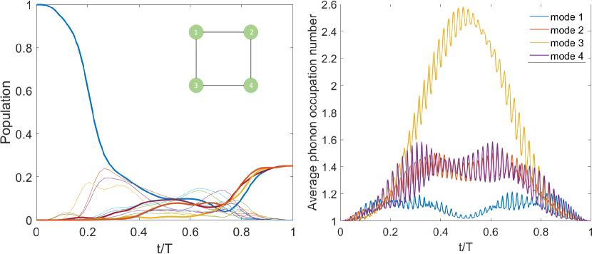
Figure 7: Numerical simulation of a four ion gate which implements a cluster state coupling map (inset of left plot). Left: The population of each spin basis state over the duration of the gate; bold lines correspond to states with non-zero amplitude at the gate time. Right: average occupation number of each phonon mode over the duration of the gate. The values shown here are well below $N_{\text{cutoff}}=14$.

We use this to simulate the solutions obtained by our method above, on a four ion system. We observe a very good agreement between the fidelity obtained through the simulation and that predicted by Eq. (8). As an example, we highlight a gate which implements the four-ion “cluster state.”

Figure 7 (left) shows the populations of each spin basis state over the duration of the gate, as determined by the simulation; the target final state is $\ket{\psi}=\frac{1}{2}(\ket{0000}-\ket{0110}-\ket{1001}-\ket{1111})$. Also shown in Figure 7 (right) is the average phonon occupation number for each of the four motional modes.

The phonon cutoff we use is $N_{\text{cutoff}}=14$, which is justified by the fact that phonon states above $n=10$ are hardly populated at all, i.e. $\sum_{n>10}\bra{n}\rho_{\text{motion}}(t)\ket{n}<10^{-5}$.

For this gate the fidelity returned by the simulation is $99.987\%$, nearly identical to the value predicted by Eq. (8). This is the ideal case, which is also solved analytically, however the simulation also allows us to consider potential sources of error. For example we can add a carrier coupling term to the Hamiltonian:

$$H_{\text{c.c}}=2\sum_{n=1}^{N}\sum_{m=1}^{M}\sigma_{y}^{(n)}\text{cos}(\omega_{m}t)\left(\bm{r}_{n}\right)_{m}$$ (18)

We note that due to the $\sigma_{y}$ operators, the addition of this term breaks our assumption that the Hamiltonian can be decomposed to a sum of commuting terms. Thus we heuristically account for carrier coupling by considering $H_{j}\rightarrow H_{j}+\frac{1}{N}H_{\text{c.c}}$. Accounting for carrier coupling, the simulation gives essentially the same fidelity. We note that carrier coupling generally has a greater impact on the gate fidelity when working with smaller motional frequencies. However, if necessary, robustness against carrier coupling could always be further improved by imposing additional linear constraints.

Figure 8: Fidelities of multiple four-ion gates (corresponding to either a cluster state or all-to-all coupling map), each with a different gate time. For each gate, three values of the fidelity are shown: estimated with Eq.(8) (blue), calculated from the simulation in the ideal case (orange), calculated from the simulation while accounting for both carrier-coupling as well as higher-order Lamb-Dicke errors (yellow). It is clear that the fidelity determined by the simulation is very close to the estimated value. Moreover, the errors considered here do not have a significant effect on the fidelity.

Furthermore, we study the effect of higher order Lamb-Dicke terms in the Hamiltonian. Specifically we consider terms that modify the first-order sideband interaction (not spin squeezing terms). We do so by modifying the phonon creation and annihilation operators in the Hamiltonian to include $O(\eta^{2})$ terms in the Debye-Waller factor [34]. With these terms included, the simulation fidelity is essentially unchanged; we note that these terms are expected to have a negligible contribution, as $\eta^{2}\approx 10^{-4}$.

Figure 8 shows fidelities determined by the simulation of multiple four-ion gates, corresponding to the $N=4$ gates in Fig. 1, both for the ideal case as well considering the two error sources mentioned above, compared with our method’s expected fidelity as defined in Eq. (8).

Appendix F: Quantifying mode and ion position variance

The unitary evolution operators allow for calculating the position and momentum expectation values of the motional modes as well as individual ions in the ion crystal. Here we provide the expressions used for the analysis of ion and mode motion, shown in Fig. 4, above.

For simplicity, we assume that the initial state of all modes of motion is the ground state, $n_{j}=0$. Moreover, we assume the initial spin state is in the Pauli-$x$ basis, $\ket{s_{1},...,s_{N}}$, i.e. with $s_{n}=\pm 1$ signifying the $\pm 1$ single-qubit eigenstates of $\sigma_{x}$. Due to the unitary evolution operator in Eq. (13), the expected value of displacement of the $j$th mode in this state, is given by

$$\expectationvalue{x_{j}}_{t}=\sum_{n=1}^{N}2s_{n}\real\left[\alpha_{j}^{\left(n\right)}\left(t\right)\right],$$ (19)

with $\alpha_{j}^{\left(n\right)}$ define in Eq. (14) above. The initial qubit computational ground state, is a state in which all qubits are set to $\sigma_{z}=1$, and is an equal superposition of all $\ket{s_{1},...,s_{N}}$ states. Thus the expectation value of the qubit ground state will vanish, due to the summation of $s_{n}=\pm 1$ for all $n$.

Therefore a better quantifier for displacement of the the phonon mode, during gate operation, is the mode variance, given by,

$$\expectationvalue{x_{j}^{2}}_{t}=\frac{1}{2^{N}}\sum_{\bm{s}\in\{+1,-1\}^{N}}\left(\sum_{n=1}^{N}2s_{n}\real\left[\alpha_{j}^{\left(n\right)}\left(t\right)\right]\right)^{2},$$ (20)

where the first sum is on all possible $\ket{s_{1},...,s_{N}}$ states. This is simplified to,

$$\expectationvalue{x_{j}^{2}}_{t}=4\sum_{n=1}^{N}\left(\real\left[\alpha_{j}^{\left(n\right)}\left(t\right)\right]\right)^{2},$$ (21)

The expected position of the $n$th ion, $X_{n}$, is given by, $\expectationvalue{X_{n}}=\sum_{j=1}^{N}O_{j}^{\left(n\right)}\expectationvalue{x_{j}}$. Since in the spin ground state all mode expectation values vanish, then so does the expected ion position. Here as well we instead use the position variance, yielding,

$$\expectationvalue{X_{n}^{2}}=\sum_{j=1}^{N}\left(O_{j}^{\left(n\right)}\right)^{2}\expectationvalue{x_{j}^{2}}_{t}.$$ (22)

The expression in Eq. (22) is used in order to generate Fig. 6 of the main text.

Appendix G: Comparison of zero phase solutions using global addressing and multi-addressing ansatz

As described in the main text, we aggregate zero-phase solutions under the assumption that the ions are driven by a global beam, equally illuminating all ions. This results in only $N$ quadratic constraints, and has solutions, $\bm{z}_{\text{g}}\in\mathbb{R}^{M}$. These solutions are then used as zero-phase solutions for independently addressed ions, as $\bm{z}_{n}=\bm{z}_{\text{g}}$ for all $n=1,..,N$. Since these zero-phase solutions originate from a subspace of the full optimization problem search space, i.e. they have $M$ degrees of freedom, instead of $N\times M$, then they might result in sub-optimal converted solutions.

Here we use a small-size system in order to exemplify that the performance of solutions originating from a global zero-phase solution, is in effect as good as that of solutions based on $N\times M$ degrees of freedom. To do so we use a small, nine ion, crystal. We generate 50 zero-phase solution using a global assumption (with $9$ quadratic constraints), $\bm{z}_{\text{g}}$ and 50 zero-phase solutions, assuming independent, multi-addressing of the ions (with $9\times 8/2=36$ quadratic constraints), $\bm{z}$. These solutions are then converted to full solutions of various random targets, $\bm{r}_{\text{g}}$ and $\bm{r}$ respectively.

All of the converted solutions yield high-fidelity entanglement gates, which satisfy the infidelity criterion, set here intentionally high, to $10^{-8}$. Figure 9 (left) shows a comparison of the total required Rabi frequency of both types of zero-phase solution ansatze. Each point corresponds to a random target positioned according to its square root absolute nuclear-norm $\sqrt{\text{nuc}\left(\left|\varphi_{n,m}\right|\right)}$ and $\left|\bm{r}\right|$ scaled by the frequency of the first mode of motion, $\nu_{1}$ (vertical). Solutions converted from a global ansatz (blue) require a drive power that is almost equal to those converted from an independent ansatz (orange). We note that a similar behavior is exhibited in terms of fidelity. This indicates that the independently driven zero-phase solutions do not provide superior converted solutions.

We furthermore study correlations between the solutions. We choose the right-most entanglement target, in Fig. 9, and for each multi-addressed zero-phase solution, $\bm{z}$ we find an extended globally addressed zero-phase solution, $\tilde{\bm{z}}_{\text{g}}=\begin{pmatrix}\bm{z}_{\text{g}}&\bm{z}_{\text{g}}&\cdots&\bm{z}_{\text{g}}\end{pmatrix}\in\mathbb{R}^{NM}$ which is ’closest’ to it in terms of overlap in aboslute value, i.e. that maximizes the quantity $o_{z}\equiv\left|\tilde{\bm{z}}_{\text{g}}\cdot\bm{z}\right|/\left|\tilde{\bm{z}}_{\text{g}}\right|\left|\bm{z}\right|$. We plot these overlaps on Fig. 9 (right) on the horizontal axes. We compare to the same overlap of the converted solutions (vertical). We observe a low overlap between zero-phase solutions and a high overlap between full solutions, meaning that the while the zero phase solutions of both methods yielded different results, many converted solutions converge to the same locally optimal solution.

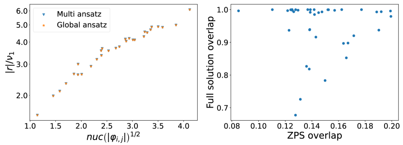
Figure 9: Comparison of zero-phase solutions using global addressing and multi-addressing ansatz. Left: Total Rabi frequency required by the two approaches. For each target (point) we present the average Rabi frequency for the converted global ansatz (orange) and multi-addressed independent ions ansatz (blue). Showing an agreement between both ansatze. Right: Overlap between the two types of anstaz for a specific target realization. Showing the closest overlap between zero-phase solutions on the horizontal axis and the overlap of the corresponding full solution in the vertical.