capbtabboxtable[][]

Transient Neural Radiance Fields
for Lidar View Synthesis and 3D Reconstruction
–Supplementary Material–

1 Hardware Prototype

To create the captured dataset, we built a hardware prototype consisting of a pulsed laser (NKT Photonics Katana 05HP) operating at 532 nm that emits 35 ps pulses of light at a repetition rate of 10 MHz. The output power of the laser is lowered to $<1$ mW to keep the flux low enough (roughly $150,000$ counts per second on average) to prevent pileup, which is a non-linear effect that distorts the SPAD measurements [1]. The laser emits polarized light that passes through a polarizing beam splitter (Thorlabs PBS251), to a set of 2D scanning mirrors (Thorlabs GVS012). The mirrors are controlled by a multifunction I/O device (NI-DAQ USB-6343) and are used to scan scenes at a spatial resolution of 512$\times$512 at a rate of 0.1 frames per second. The laser shares an optical path through the beam splitter with a single pixel SPAD (Micro Photon Devices PDM series SPAD) with a 50 $\mu$m $\times$ 50 $\mu$m active pixel area. Photons detected by the SPAD are correlated with a sync signal from the laser using a time-correlated single photon counter (TCSPC) to measure the photon arrival timestamps.

We place the scanned scenes on a rotation stage (Parker Motion/Parker 6K4 Compumotor) in front of the scanning single-photon lidar, allowing us to capture different viewpoints by rotating the scene.

Each scan consists of 20 minutes of total exposure time, but we save out all collected photon timestamps individually so that any desired exposure time can be emulated by accumulating photons over the desired time window in post processing (i.e., for future applications of the dataset). We set the bin width of the photon count histograms to 8 ps and the number of bins is 1500. The entire data acquisition is controlled using custom-developed MATLAB software on a desktop PC, and we capture six scenes with varying geometry, texture, and material properties. For each scene, we capture views in 18 degree increments of the rotation stage, resulting in a 360 degree capture. We set aside 8 views for training, and 10 separate views sampled in 36 degree increments comprise the test split. Prior to input into the network for training, we normalize the measurement values by the maximum photon count observed across all views.

2 Calibration of the Hardware Prototype

Here we describe the method used to find the extrinsics and intrinsics defining the captured dataset. An overview of the method can be found in the Algorithm 4.

Intrinsics. We calibrate the camera intrinsics of the system using the raxel model [2], which maps each pixel to a 3D ray direction. To find the ray directions, we place a checkerboard on a translation stage and use the lidar system to capture two images of this checkerboard before and after translating $17$ cm by in the direction of the surface normal of the board (this was the maximum distance permitted by the translation stage and our optical table layout).

Checkerboard corners are detected in the two images using OpenCV’s findChessboardCorners [3] with subpixel refinement. In order to improve robustness to distortion, we further refine the corner detection by fitting a second-order polynomial to corners along vertical lines (which we found to be a good fit to model the observed distortion), and we use a first-order fit to horizontal lines, which we found to fit the data well. We set the corner positions to the intersections of the set of fitted lines.

The pixel coordinates of the detected checkerboard corners are then used to define a 3D coordinate system. We set the origin of the coordinate system to the upper-left corner of the nearest checkerboard, and coordinates on the far checkerboard are calculated based on the known translation in $z$, with $x$ and $y$ coordinates given using the size of the checkerboards (4.2 mm). We associate ray directions to each pixel by finding the points of intersection of the ray with the two checkerboards. Specifically, we linearly interpolate the mapping from pixel values to 3D coordinates at each checkerboard corner to retrieve a dense mapping from pixels to 3D coordinates on each board. Then, for a given pixel the ray direction is given by a simple subtraction of the 3D intersection points on each board.

Extrinsics. Our captured dataset consists of photon count histograms from six different scenes, each with 20 different views. We use a rotation stage to move the scenes one full revolution in 18 degree increments. The resulting views are equivalent to capturing a stationary scene with cameras that are rotated about the center of rotation of the stage. Since all scenes are captured identically in this fashion, we determine the camera extrinsics once for all scenes.

We also calibrate for an additional offset parameter to finetune the time-of-flight-delays recorded by the lidar system. This accounts for the unknown time delay between the time that the time-correlated single-photon counter receives the sync signal from the laser and the time that the laser pulse reaches the center of projection of the scanning mirrors. In other words, this offset accounts for when “time zero” should occur in the photon count histograms; we roughly calibrate for this value by placing a target directly in front of the galvo mirrors, and we fine tune this offset via optimization as detailed below.

Given that each view is captured using a controlled rotation, the extrinsics can be determined by identifying the 3D axis of rotation and 3D center of rotation. To estimate these parameters, we use a two step procedure. First, we capture lidar scans of a checkerboard placed on the rotation stage and rotated to 6 different positions in 9 degree increments. We convert the lidar scans to a point cloud using the raxel model and lidar time of flight, and then a coarse solution is obtained by fitting planes to the point clouds and finding the center and axis of rotation that align the plane normals. Second, we detect corners of the checkerboards and find the corresponding 3D points. Then, we optimize for the center of rotation, axis of rotation, and the 1D offset parameter that best align the 3D checkerboard corners.

Specifically, we implement a routine in PyTorch [4] to align the 3D checkerboard corners using the Rodrigues formula given below.

$$\mathbf{v^{\prime}}=(\mathbf{v}-\mathbf{c})\cos\theta+(\mathbf{a}\cdot(\mathbf{v}-\mathbf{c}))(1-\cos\theta)\,\mathbf{a}+(\mathbf{a}\times(\mathbf{v}-\mathbf{c}))\sin\theta+\mathbf{c}.$$ (1)

Here, $\mathbf{v}$ is the 3D point to be rotated, $\mathbf{c}$ is the center of rotation, $\mathbf{a}$ is the axis of rotation, and $\mathbf{v^{\prime}}$ is the rotated point. We minimize the objective function given as

$$\mathcal{L}_{\text{align}}=\sum\limits_{p}\sum\limits_{[i,j]\in\mathcal{C}}\lVert\mathbf{v^{\prime}}^{(i)}_{p}-\mathbf{v^{\prime}}^{(j)}_{p}\rVert_{2}^{2},$$ (2)

where $p$ indexes the checkerboard corner points and $[i,j]$ index all pairs of checkerboards. Thus we penalize the distance between corresponding points between all checkerboards. The optimization is performed using LBFGS [5]. After optimization, we use the resulting center point and rotation matrices (i.e., by rotating around $\mathbf{a}$ by increments of 18 degrees) to define the camera extrinsics for each view.

 Intrinsics Calibration

 Data: Two scans of a checkerboard before and after translation.

1. Perform sub-pixel detection of checkerboard corners using OpenCV and polynomial line fitting.

Use the detected checkerboard corners to initialize a 3D coordinate system.

Compute per-pixel 3D coordinates for each checkerboard scan by interpolating the mapping from corner pixel coordinates to 3D coordinates.

Compute the ray directions by subtracting the per-pixel 3D coordinates obtained for the checkerboard scan before and after translation.

  Extrinsics Calibration

  Data: Six scans of a checkerboard rotated using the rotation stage.

1. Convert lidar scans to point clouds using the time of flight and intrinsics.

Fit planes and determine initial center and axis of rotation to align the surface normals.

Detect 3D points corresponding to checkerboard corners.

Refine the initial center and axis of rotation via Equations 1 and 2.

Algorithm 1 Calibration overview.

3 Additional Implementation Details

Network Architecture. In this section we describe the main network architecture. We extend the NerfAcc [6] framework and the provided implementation of Instant-NGP (INGP) [7]. All network hyperparameters are shared between our proposed method and the baselines unless otherwise stated. We set the number of hash feature grids for INGP to 16 and set the feature size to 2. The resolution of the coarsest grid is set to $16$ and each subsequent grid has $2$ times finer resolution. The base MLP has width $64$ with 1 hidden layer to map to density and a latent vector. Another MLP with $2$ hidden layers and $64$ hidden units maps from the latent vector and viewing direction to the view-dependent radiance.

We use the occupancy grid from NerfAcc with a resolution of $128^{3}$. The occupancy grid is employed to remove samples along the ray based on their density for the sake of efficiency. The grid is binarized using a occupancy value of $10^{-3}$.

For the captured data, we find that setting the binarization threshold to $10^{-5}$ for the first 3,000 iterations before reverting back to the standard $10^{-3}$ value helps to avoid an overly aggressive removal of density that erodes the surface of reconstructed objects. In addition, we incorporate pruning based on transmittance, removing any samples that register a transmittance of 0 to speed up rendering. Finally, all rays are rendered by sampling 4,096 points along each ray, and these points are pruned according to their occupancy and transmittance values, as previously discussed.

We set the bounding box used in INGP as follows for the simulated and captured data. For the simulated data the bounding box extents are set to -1.5 to 1.5 across all dimensions and methods. For captured data, we use a -0.4 to 0.4 bounding box for Transient NeRF; we slightly shrink the bounding box for baselines run on captured data to -0.3 to 0.3, which we find helps remove some spurious regions of density and improves the baseline results.

Optimization settings and run time. The time required for training is strongly influenced by the number of samples used for the spatial filter, as discussed in the main text. Specifically, each image pixel is rendered by computing a weighted integral over the radiance for a particular region of space. We compute this integral during training by stochastically sampling one or more ray directions per pixel with probability determined by the weighting and support of the spatial filter [8]. For the simulated dataset, we initially sample a single ray for the first 2000 iterations, then subsequently double this number every 2000 iterations until we reach a maximum of 30 rays sampled per pixel. For the captured dataset we use a single ray sample per pixel per iteration; we find that increasing the number ray samples results in longer training times without significantly improved performance.

Training takes roughly eight hours to converge for the simulated dataset (250K iterations) and two hours to converge for captured data (150K steps).

Depth calculation. We follow the NeRF convention in calculating depth for all baseline methods as

$$d=\sum_{i}\sigma(t_{i})T(t_{i})\frac{t_{i}+t_{i+1}}{2},$$ (3)

where $t_{i}$ is the distance from the ray origin to a sample along the ray, $T_{i}$ is the transmittance, and $\sigma$ is the density. Intuitively, this equation calculates the expected ray termination distance.

Since our method incorporates a spatial filter to more accurately model the footprint of the illumination spot, a single ray can result in measurements from multiple surfaces (e.g., if a pixel integrates over a depth discontinuity). To avoid multiple depths in the measurement from skewing the estimate of the expected ray termination distance, we use the following equation to compute depth.

$$d=\arg\max_{t_{i}}\sigma(t_{i})T(t_{i})$$ (4)

Thus, we find the depth at which the maximum probability of ray termination occurs.

We note that in the conventional NeRF depth rendering formula of Equation 3, regions of low density become less visible in most visualizations because their depth tends towards zero (i.e., it is weighted by the density, which is close to zero, but typically not uniformly zero for empty regions). However, in Equation 4, no such weighting exists, resulting in visualizations that appear noisier because depths for regions with low (but non-zero) density are not automatically suppressed. Thus for visualization of the depth maps we weight the depth as follows.

$$d=\left(\sum_{i}\sigma(t_{i})T(t_{i})\right)\arg\max_{t_{i}}\sigma(t_{i})T(t_{i}).$$ (5)

We use this equation to visualize depth maps, as we find they are more comparable to those rendered with the conventional NeRF formulation (though the density and transmittance weighting results in them being slightly less accurate).

3.1 Baselines Implementation Details

Four different baselines are implemented to evaluate our proposed method. To isolate the impact of different loss functions and speed up the training, we implemented the specific loss functions from each of the following methods in the framework of NerfAcc with the Instant-NGP backbone.

For all baselines, we generate the ground truth intensity images by first integrating the transients over the time dimension and normalization by a scale factor to shift the image values to lie close to within [0, 1]. We apply gamma correction to tonemap the resulting high dynamic range intensity images prior to training.

Instant-NGP [7]. The Instant-NGP model is trained with photometric loss defined as the total squared error between the rendered intensities and the pixel colors from the input images:

$$\mathcal{L}_{\text{photo}}=\sum_{\mathbf{r}\in\mathcal{R}}\rVert\widetilde{\mathbf{C}}(\mathbf{r})-\mathbf{C}(\mathbf{r})\lVert_{2}^{2}$$ (6)

where $\widetilde{\mathbf{C}}$ and $\mathbf{C}$ denote the ground-truth pixel color and the predicted value, respectively. $\mathcal{R}$ specifies the set of active rays that have non-zero opacity values; this set of rays is updated as training progresses to accelerate optimization by pruning rays that do not contribute to the rendering [6].

Depth-Supervised NeRF [9]. Following the depth supervision idea proposed in  [9], we train a new model that incorporates depth error loss in addition to the photometric loss above:

$$\mathcal{L}_{\text{depth}}=\frac{1}{|\mathcal{R^{\prime}}|}\sum_{\mathbf{r}\in\mathcal{R^{\prime}}}\big{(}\widetilde{d}(\mathbf{r})-d(\mathbf{r})\big{)}^{2}$$ (7)

$\widetilde{d}(\mathbf{r})$ denotes the lidar depth for ray $\mathbf{r}$ obtained from the captured transients using a log-matched filter [10], $d(\mathbf{r})$ is the predicted depth value computed from Equation 3, and $\mathcal{R^{\prime}}$ specifies the set of rays that intersect with the object.

The final training loss is defined as $\mathcal{L}=\mathcal{L}_{\text{photo}}+\lambda_{\text{depth}}\mathcal{L}_{\text{depth}}$. In the simulated and captured results, $\lambda_{\text{depth}}$ is set to $0.005$ and $0.0075$, respectively.

Urban NeRF [11]. We further incorporated the line-of-sight lidar loss $\mathcal{L_{\text{sight}}}$, proposed in  [11], to encourage the densities to be concentrated near the lidar points. This loss comprises two terms. The first term penalizes any density between the ray origin and the lidar point:

$$\mathcal{L}_{\text{empty}}=\frac{1}{|\mathcal{R^{\prime}}|}\sum_{\mathbf{r}\in\mathcal{R^{\prime}}}\big{[}\int_{t_{n}}^{\widetilde{d}-\epsilon}w(t)^{2}dt\big{]}.$$ (8)

$\mathcal{R^{\prime}}$ is the set of rays that intersect with the object; $w(t)$ is the volume rendering integration weights defined as $\sigma(t)T(t)$; $t_{n}$ denotes the near bound of the ray; and $\epsilon$ specifies a neighbourhood around the surface point.

The second term, on the other hand, encourages the model to increase the densities in the bounded region around the surface point:

$$\mathcal{L}_{\text{near}}=\frac{1}{|\mathcal{R^{\prime}}|}\sum_{\mathbf{r}\in\mathcal{R^{\prime}}}\big{[}\int_{\widetilde{d}-\epsilon}^{\widetilde{d}+\epsilon}(w(t)-\mathcal{K}_{\epsilon}(t-\widetilde{d}))^{2}dt\big{]}$$ (9)

where $\mathcal{K}_{\epsilon}$ is a truncated Gaussian defined as $\mathcal{N}(0,(\epsilon/3)^{2})$ [12].

The final training loss for this model is defined as:

$$\mathcal{L}=\mathcal{L}_{\text{photo}}+\lambda_{\text{depth}}\mathcal{L}_{\text{depth}}+\lambda_{\text{sight}}\mathcal{L}_{\text{sight}}$$

where $\mathcal{L}_{\text{sight}}=\mathcal{L}_{\text{empty}}+\mathcal{L}_{\text{near}}$. The parameters $(\lambda_{\text{depth}},\lambda_{\text{sight}})$ are set to $(0.0001,0.005)$ for both the simulations and captured experiments.

Following the instructions from the original paper, we applied exponential decay to the value of $\epsilon$ throughout the optimization, which encourages the density of the radiance field to fall within a progressively smaller support, improving convergence. We initialize $\epsilon$ to a value $\epsilon_{\text{max}}$, and every $7000$ steps we multiply by a factor of $0.8$, until it decays to $\epsilon_{\text{min}}$. Parameters $(\epsilon_{\text{max}},\epsilon_{\text{min}})$ are set to $(1.5,0.025)$ and $(4.0,0.05)$ for the captured and simulated results, respectively.

Urban NeRF with Masking. The depth-related loss terms $\mathcal{L}_{\text{depth}}$ and $\mathcal{L}_{\text{sight}}$ used in the previous two models are evaluated only for the rays that intersect with the object; however, we find that the included regularization terms do not prevent spurious regions of density that appear for pixels that fall outside the support of the object on the image plane.

We attempt to improve the baseline results further by using modified versions of $\mathcal{L}_{\text{photo}}$ and $\mathcal{L}_{\text{sight}}$ which sum over active rays $\mathcal{R}$. Specifically we use an oracle object mask (i.e., a ground truth mask segmenting the object in each training view) and set the ground truth depth of all background pixels to zero. This loss encourages the density to be uniformly zero along background rays and helps to remove spurious clouds of density that tend to materialize in the other baseline results during training. We note that this masking loss is directly analogous to the sky modeling loss proposed in Urban-NeRF [11], which penalizes density along rays that intersect with the sky as determined using a semantic segmentation network.

For both the simulated and captured results, we hand-annotate the oracle object masks by carefully thresholding the intensity images and applying morphology operations to fill in holes in the mask.

4 Supplemental Results

4.1 Dataset

Simulated dataset. To create the simulated multiview lidar dataset, we modify the Non-Line-of-Sight (NLOS) Mitsuba 2 rendering codes of Royo et al. [13]. While the original codebase enables one to simulate the effect of illuminating a single point in the scene with a laser and imaging other points, our approach requires rendering a frame where each pixel images an area of the scene that is illuminated with a coaxial, collimated light source. To this end, introduce a new light source as well as additional rendering options such that each pixel is rendered independently with its own coaxial light source. We also incorporate a Gaussian reconstruction filter [8] along the time dimension to avoid aliasing or stair-stepping artifacts in regions with fine variations in depth.

We choose the variance of the Gaussian temporal filter and spatial filters to produce transients that measure a laser pulse with similar temporal and spatial support as the captured results. Specifically, we set the variance of the temporal and spatial filters to $3$ and $0.15$ respectively. We simulate photon count histograms $1200$ bins and each bin has a width of approximately $\sim 30ps$.

We subsample 8 training viewpoints from the simulated lidar measurements rendered at 36 degree increments along a circle centered at the origin. Specifically, we sample 2 views separated by 180 degrees; 3 views separated by 90 and 180 degrees (i.e., a superset of the 2 views), and 5 views uniformly separated by 72 degrees. Note that the 5 views are not a superset of the viewpoints used when training on 2 or 3 lidar measurements. For testing, we use 6 viewpoints from the NeRF Blender test set that surround the object.

Captured dataset. The captured dataset consists of 20 multiview single-photon lidar scans of six scenes. The scenes consist of everyday objects and figurines (see Fig 1). We record photon timestamps at 4 ps resolution for each scene, with measurements of each view being captured during an exposure period of 20 minutes. While we use all photon timestamps in the photon count histograms used for the proposed method, access to the photon timestamps also allows synthesizing histograms with arbitrary exposure time, which will make the dataset useful for a wide array of follow-on work.

We use raw photon count histograms with 4096 bins and bin widths of $4$ ps. To decrease the memory required for training, we crop and downsample the histograms to $1500$ bins with $8$ ps resolution.

Measurements are captured in the low-flux regime to avoid non-linear distortions due to pile-up. A detailed breakdown of the photon counts and acquisition parameters for each captured scene is provided in Table 1.

scene name	spatial resolution	histogram bins	exposure time/view	avg. counts/view	avg. counts/sec
baskets	512$\times$ 512	1500	20 min	9.04$\times 10^{7}$	7.53$\times 10^{4}$
boots				7.39$\times 10^{7}$	6.16$\times 10^{4}$
carving				5.60$\times 10^{7}$	4.66$\times 10^{4}$
chef				2.56$\times 10^{8}$	2.13$\times 10^{5}$
cinema				1.51$\times 10^{8}$	1.26$\times 10^{5}$
food				1.44$\times 10^{8}$	1.20$\times 10^{5}$

Table 1: Photon counts per scene for the captured dataset.

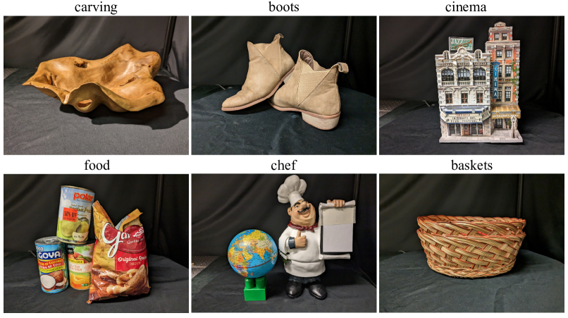
Figure 1: The captured dataset. The captured datset consists of 20 multiview single-photon lidar scans of six scenes.

4.2 Ablation Studies

In Table 2 we show ablation studies of our method calculated on the captured cinema scene. Specifically, we include quantitative results of our method without the space carving loss and without accounting for the laser profile via convolution as described in the main text.

The space carving loss appears to especially improve performance in the five view case. It helps eliminate spurious clouds of density, which improves reconstruction quality for held-out test views.

We also note the importance of explicitly accounting for the laser pulse width and system jitter. This is especially noticeable for the two view results, where the depth becomes highly skewed without this component. We attribute this effect to a thickening of the density representing the object surface; the optimization appears to converge to this solution to explain the temporal spread of the returning light captured in the photon count histograms. Properly accounting for the laser pulse and system jitter essentially deconvolves the temporal response of the lidar system, resulting in thin sheets of density that accurately localize the object surface.

Table 2: Ablation studies on our method for the captured cinema scene. We present results while ommiting any temporal filtering (/wo tf) and omtting the space carving loss (/wo sc).

	PSNR (dB)$\,\uparrow$			LPIPS$\,\downarrow$			SSIM$\,\uparrow$			L1 (depth) $\,\downarrow$
Method	2 views	3 views	5 views	2 views	3 views	5 views	2 views	3 views	5 views	2 views	3 views	5 views
Our method /wo tf	16.55	20.85	20.02	0.346	0.225	0.209	0.589	0.837	0.823	0.022	0.007	0.009
Our method /wo sc	20.63	21.09	20.12	0.207	0.200	0.217	0.855	0.855	0.840	0.007	0.009	0.020
Our method	21.61	21.66	25.12	0.281	0.245	0.178	0.850	0.812	0.879	0.006	0.006	0.007

4.3 Simulated Results

In Figs. 2, 3, and 4 we show further renders from our method and baseline methods trained on the simulated dataset. The same trends as in the main text persist. Our method qualitatively produces images more faithful to the ground-truth. Our rendered images suffer less from floating artifacts and display finer details, for example in the lego scene. Some artifacts in the depth maps (i.e., the "holes" that appear) result from how we visualize depth in low occupancy areas. Depths in these regions can be become biased as described by Equation 5.

We show a breakdown across all simulated scenes of the evaluation metrics (see Table 3,  4,  5,  6). In addition to the metrics reported in the main text (PSNR, LPIPS, L1 depth) we add the structural similarity (SSIM) metric. Again, our method outperforms the baselines in the quantitative metrics. Since the 2, 3, and 5 view results do not include viewpoints that are strict supersets of each other, the performance of some metrics does not always increase for every scene in every case with increasing views (though this is a trend we observe on average).

Table 3: Breakdown of PSNR (dB) across all 5 simulated scenes.

	Instant NGP [7]$\,\uparrow$			DS-NeRF [9]			Urban NeRF  [12]			Urban NeRF w/Mask [12]			Proposed
Scene	2 views	3 views	5 views	2 views	3 views	5 views	2 views	3 views	5 views	2 views	3 views	5 views	2 views	3 views	5 views
lego	16.04	17.46	16.46	17.66	19.45	17.21	19.59	19.75	16.19	20.48	21.50	19.48	20.64	23.63	25.81
chair	13.40	15.42	24.95	16.51	16.72	25.49	17.53	16.14	24.28	20.39	18.69	28.23	20.75	21.99	34.48
hotdog	14.95	14.72	13.80	18.93	17.47	19.12	15.75	16.37	18.04	18.90	18.71	19.53	20.74	22.64	32.36
bench	16.85	19.33	15.58	19.87	20.34	15.69	19.12	19.52	14.56	20.64	21.55	17.57	20.20	23.06	21.57
ficus	21.87	21.40	27.50	23.44	22.75	27.85	22.32	21.88	25.91	24.12	23.58	26.87	24.57	26.10	27.70
average	16.62	17.67	19.66	19.28	19.35	21.07	18.86	18.73	19.80	20.91	20.81	22.34	21.38	23.48	28.39

Table 4: Breakdown of LPIPS metric across all 5 simulated scenes.

	Instant NGP [7]$\,\uparrow$			DS-NeRF [9]			Urban NeRF  [12]			Urban NeRF w/Mask [12]			Proposed
Scene	2 views	3 views	5 views	2 views	3 views	5 views	2 views	3 views	5 views	2 views	3 views	5 views	2 views	3 views	5 views
lego	0.591	0.544	0.479	0.500	0.476	0.482	0.519	0.522	0.503	0.471	0.442	0.421	0.190	0.161	0.192
chair	0.501	0.466	0.296	0.482	0.461	0.306	0.494	0.474	0.326	0.359	0.357	0.275	0.138	0.138	0.037
hotdog	0.583	0.615	0.523	0.456	0.470	0.390	0.580	0.553	0.433	0.533	0.466	0.395	0.242	0.241	0.118
bench	0.538	0.442	0.398	0.444	0.422	0.459	0.502	0.473	0.483	0.400	0.368	0.375	0.194	0.139	0.159
ficus	0.387	0.311	0.238	0.272	0.352	0.244	0.403	0.400	0.286	0.287	0.278	0.229	0.094	0.079	0.069
average	0.520	0.476	0.387	0.431	0.436	0.376	0.500	0.484	0.406	0.410	0.382	0.339	0.172	0.151	0.115

Table 5: Breakdown of SSIM metric across all 5 simulated scenes.

	Instant NGP [7]$\,\uparrow$			DS-NeRF [9]			Urban NeRF  [12]			Urban NeRF w/Mask [12]			Proposed
Scene	2 views	3 views	5 views	2 views	3 views	5 views	2 views	3 views	5 views	2 views	3 views	5 views	2 views	3 views	5 views
lego	0.456	0.519	0.576	0.600	0.624	0.631	0.592	0.580	0.590	0.646	0.710	0.722	0.860	0.897	0.899
chair	0.545	0.632	0.767	0.653	0.659	0.760	0.582	0.624	0.766	0.774	0.756	0.897	0.901	0.899	0.977
hotdog	0.508	0.448	0.534	0.736	0.636	0.687	0.503	0.534	0.664	0.567	0.686	0.761	0.882	0.875	0.963
bench	0.537	0.591	0.588	0.703	0.664	0.618	0.554	0.615	0.580	0.717	0.769	0.747	0.856	0.884	0.870
ficus	0.682	0.819	0.851	0.831	0.789	0.873	0.734	0.711	0.844	0.819	0.840	0.913	0.925	0.934	0.942
average	0.546	0.602	0.663	0.705	0.675	0.714	0.593	0.613	0.689	0.705	0.752	0.808	0.885	0.898	0.930

Table 6: Breakdown of L1 (depth) metric across all 5 simulated scenes.

	Instant NGP [7]$\,\uparrow$			DS-NeRF [9]			Urban NeRF  [12]			Urban NeRF w/Mask [12]			Proposed
Scene	2 views	3 views	5 views	2 views	3 views	5 views	2 views	3 views	5 views	2 views	3 views	5 views	2 views	3 views	5 views
lego	0.224	0.236	0.195	0.136	0.127	0.193	0.105	0.100	0.151	0.040	0.049	0.057	0.023	0.011	0.008
chair	0.166	0.198	0.117	0.123	0.146	0.097	0.130	0.132	0.066	0.034	0.057	0.009	0.006	0.005	0.003
hotdog	0.344	0.254	0.271	0.131	0.151	0.115	0.301	0.270	0.089	0.126	0.040	0.008	0.007	0.006	0.003
bench	0.166	0.137	0.198	0.082	0.076	0.142	0.060	0.047	0.168	0.011	0.007	0.038	0.006	0.005	0.003
ficus	0.291	0.147	0.107	0.072	0.074	0.048	0.059	0.073	0.034	0.043	0.034	0.032	0.034	0.033	0.048
average	0.238	0.195	0.178	0.109	0.115	0.119	0.131	0.124	0.101	0.051	0.038	0.029	0.015	0.011	0.013

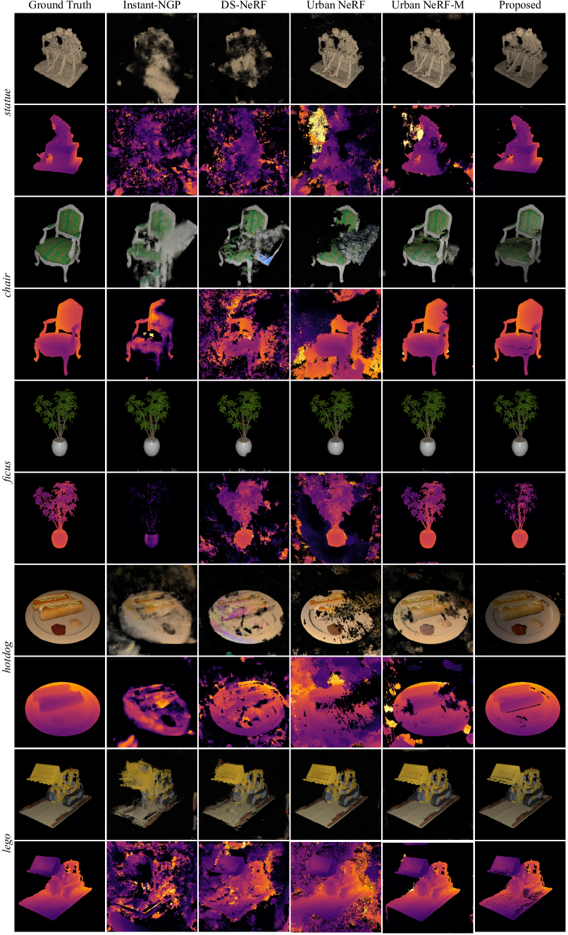
Figure 2: Rendered images and depths on the simulated dataset for 2 views.

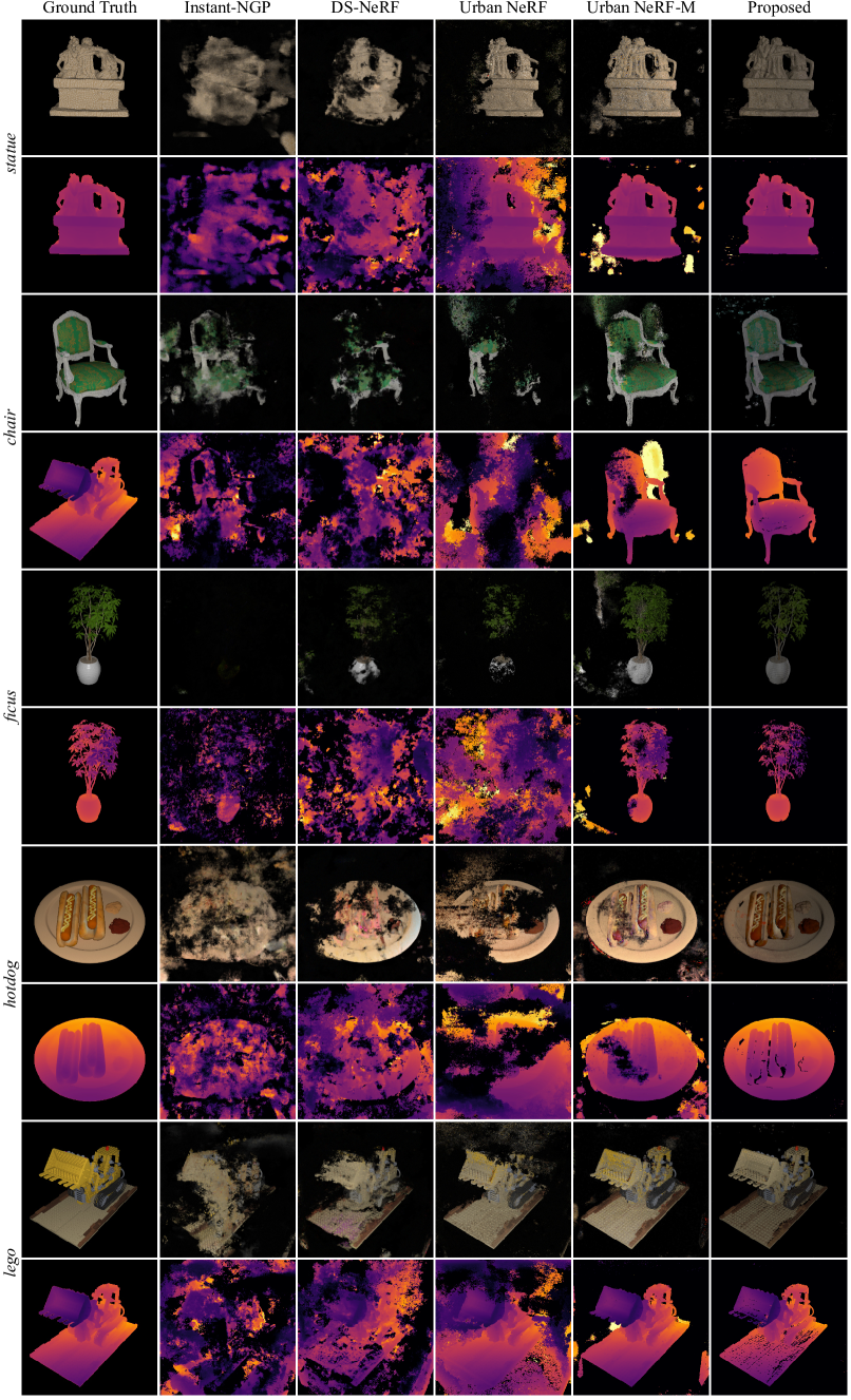
Figure 3: Rendered images and depths on the simulated dataset for 3 views.

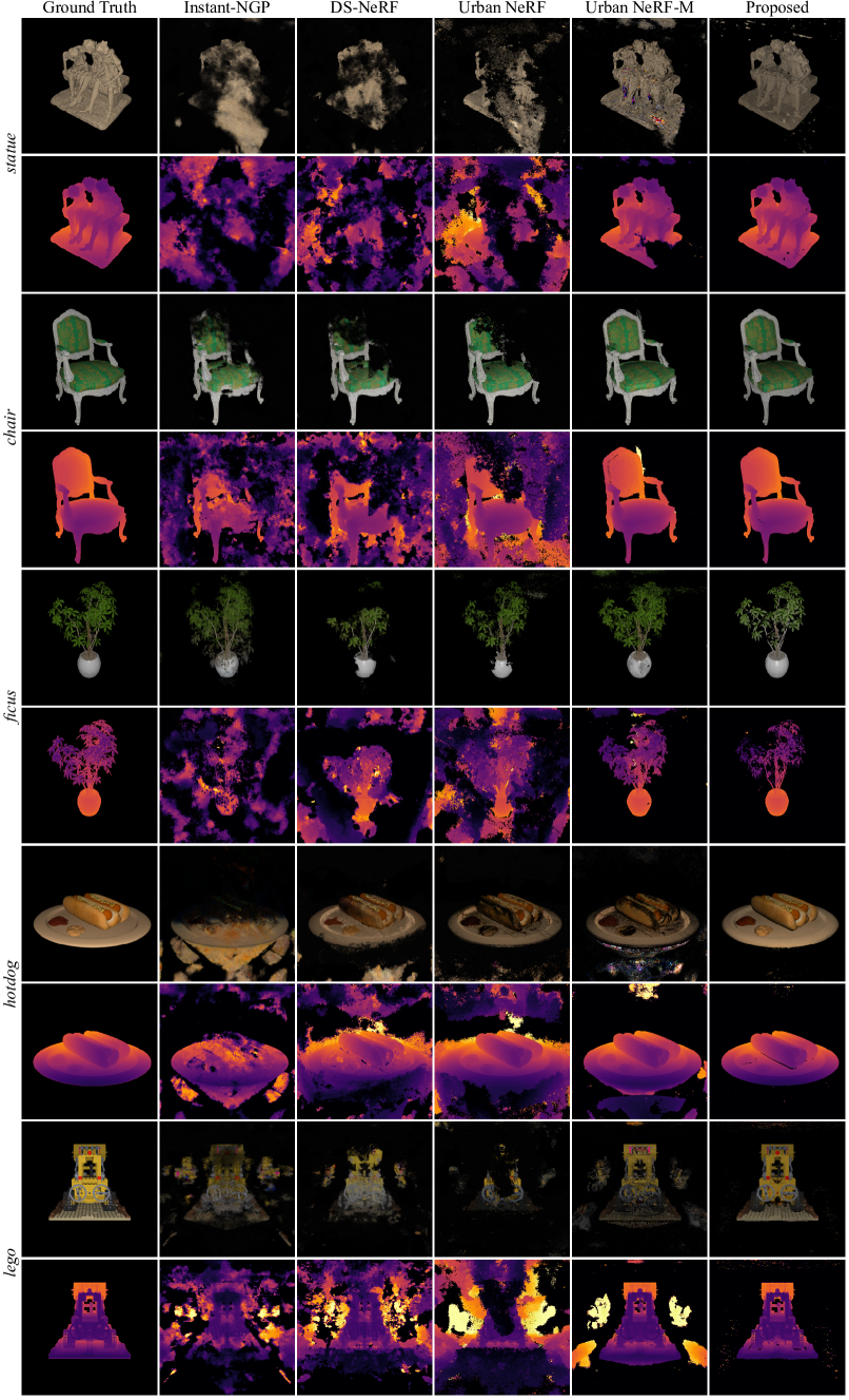
Figure 4: Rendered images and depths on the simulated dataset for 5 views.

4.4 Captured Results

In Figs. 5, 6, and 7 we show further renders from our model and the baselines on our captured dataset. The same trends as in the main text persist. Our method produces images more faithful to the ground truth.

We note that the quality of the reconstructions is lower than the simulation results. We attribute this to small imperfections in the calibration of the camera extrinsics, which register the multiview lidar scans to an accuracy of approximately 1 mm. Achieving precise, sub-mm alignment of the multiview lidar scans is a highly non-trivial problem and is outside the scope of our current work. The captured results bear out the trends observed in simulation and demonstrate Transient NeRF and novel view synthesis of lidar measurements for the first time in practice.

We show a breakdown across all captured scenes of the evaluation metrics (see Tables 7,  8,  9, and 10). In addition to the metrics reported in the main text (PSNR, LPIPS, L1 depth) we add the SSIM metric. Again our method outperforms the baselines in the quantitative metrics.

Table 7: Breakdown of PSNR (dB) across all 6 captured scenes.

	Instant NGP [7]$\,\uparrow$			DS-NeRF [9]			Urban NeRF  [12]			Urban NeRF w/Mask [12]			Proposed
Scene	2 views	3 views	5 views	2 views	3 views	5 views	2 views	3 views	5 views	2 views	3 views	5 views	2 views	3 views	5 views
cinema	14.73	15.18	15.21	13.18	13.87	12.58	17.27	15.11	17.30	14.13	17.22	17.80	21.61	21.66	25.12
boots	16.54	18.32	18.09	16.97	15.65	16.59	16.54	14.54	16.59	13.93	18.70	21.87	22.38	22.29	24.94
baskets	18.73	19.78	18.17	16.47	17.43	17.54	16.68	15.88	13.42	17.17	16.51	14.26	22.48	20.93	19.90
carving	17.96	17.30	16.70	17.41	16.36	15.44	18.71	17.97	17.36	16.07	21.41	22.28	23.52	24.20	24.70
chef	13.04	11.72	13.76	12.32	12.27	11.51	13.34	13.71	13.15	14.06	15.25	16.72	19.27	18.14	19.55
food	17.64	16.83	16.45	15.68	14.70	15.48	18.86	18.27	17.77	17.37	20.45	21.72	23.40	23.78	22.09
average	16.44	16.52	16.39	15.34	15.05	14.86	16.90	15.91	15.93	15.45	18.26	19.11	22.11	21.83	22.72

Table 8: Breakdown of LPIPS across all 6 captured scenes.

	Instant NGP [7]$\,\uparrow$			DS-NeRF [9]			Urban NeRF  [12]			Urban NeRF w/Mask [12]			Proposed
Scene	2 views	3 views	5 views	2 views	3 views	5 views	2 views	3 views	5 views	2 views	3 views	5 views	2 views	3 views	5 views
cinema	0.445	0.374	0.314	0.396	0.364	0.429	0.369	0.350	0.273	0.457	0.295	0.244	0.281	0.245	0.178
boots	0.251	0.253	0.181	0.193	0.225	0.192	0.386	0.332	0.163	0.525	0.245	0.135	0.221	0.182	0.155
baskets	0.399	0.298	0.252	0.256	0.244	0.268	0.444	0.311	0.220	0.433	0.300	0.195	0.269	0.165	0.164
carving	0.174	0.167	0.183	0.168	0.186	0.225	0.357	0.217	0.146	0.436	0.170	0.125	0.232	0.138	0.103
chef	0.580	0.443	0.401	0.498	0.434	0.467	0.513	0.468	0.362	0.473	0.373	0.270	0.334	0.338	0.276
food	0.299	0.310	0.313	0.354	0.417	0.369	0.351	0.290	0.221	0.425	0.232	0.174	0.286	0.205	0.154
average	0.358	0.307	0.274	0.311	0.312	0.325	0.403	0.328	0.231	0.458	0.269	0.191	0.271	0.212	0.172

Table 9: Breakdown of SSIM across all 6 captured scenes.

	Instant NGP [7]$\,\uparrow$			DS-NeRF [9]			Urban NeRF  [12]			Urban NeRF w/Mask [12]			Proposed
Scene	2 views	3 views	5 views	2 views	3 views	5 views	2 views	3 views	5 views	2 views	3 views	5 views	2 views	3 views	5 views
cinema	0.545	0.628	0.717	0.620	0.666	0.591	0.602	0.673	0.768	0.509	0.728	0.807	0.850	0.812	0.879
boots	0.804	0.810	0.866	0.853	0.822	0.851	0.587	0.687	0.871	0.414	0.777	0.894	0.912	0.909	0.914
baskets	0.555	0.715	0.749	0.737	0.750	0.738	0.499	0.689	0.751	0.517	0.691	0.771	0.846	0.850	0.826
carving	0.852	0.853	0.843	0.858	0.841	0.804	0.620	0.827	0.877	0.526	0.854	0.906	0.913	0.929	0.929
chef	0.414	0.586	0.647	0.544	0.608	0.574	0.450	0.559	0.686	0.488	0.651	0.780	0.775	0.747	0.811
food	0.731	0.720	0.733	0.677	0.586	0.671	0.654	0.737	0.808	0.528	0.775	0.855	0.826	0.879	0.873
average	0.650	0.719	0.759	0.715	0.712	0.705	0.569	0.695	0.793	0.497	0.746	0.836	0.854	0.854	0.872

Table 10: Breakdown of L1 (depth) metric across all 6 captured scenes.

	Instant NGP [7]$\,\uparrow$			DS-NeRF [9]			Urban NeRF  [12]			Urban NeRF w/Mask [12]			Proposed
Scene	2 views	3 views	5 views	2 views	3 views	5 views	2 views	3 views	5 views	2 views	3 views	5 views	2 views	3 views	5 views
cinema	0.141	0.052	0.041	0.067	0.040	0.050	0.023	0.017	0.015	0.018	0.005	0.006	0.006	0.006	0.007
boots	0.034	0.076	0.048	0.029	0.023	0.022	0.017	0.014	0.011	0.013	0.003	0.003	0.001	0.002	0.002
baskets	0.138	0.141	0.040	0.038	0.033	0.029	0.015	0.017	0.004	0.016	0.008	0.003	0.008	0.008	0.026
carving	0.029	0.032	0.031	0.031	0.024	0.026	0.008	0.011	0.014	0.009	0.004	0.003	0.006	0.005	0.006
chef	0.199	0.100	0.124	0.062	0.056	0.055	0.023	0.020	0.025	0.017	0.011	0.009	0.003	0.006	0.006
food	0.146	0.057	0.035	0.058	0.041	0.035	0.017	0.013	0.014	0.013	0.006	0.005	0.006	0.007	0.016
average	0.115	0.076	0.053	0.048	0.036	0.036	0.017	0.015	0.014	0.014	0.006	0.005	0.005	0.006	0.010

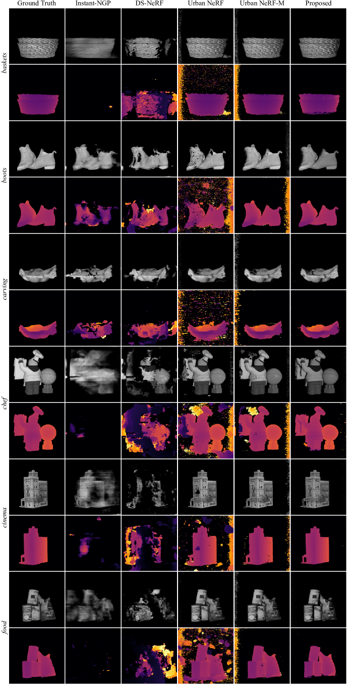
Figure 5: Rendered images and depths on the captured dataset for 2 views.

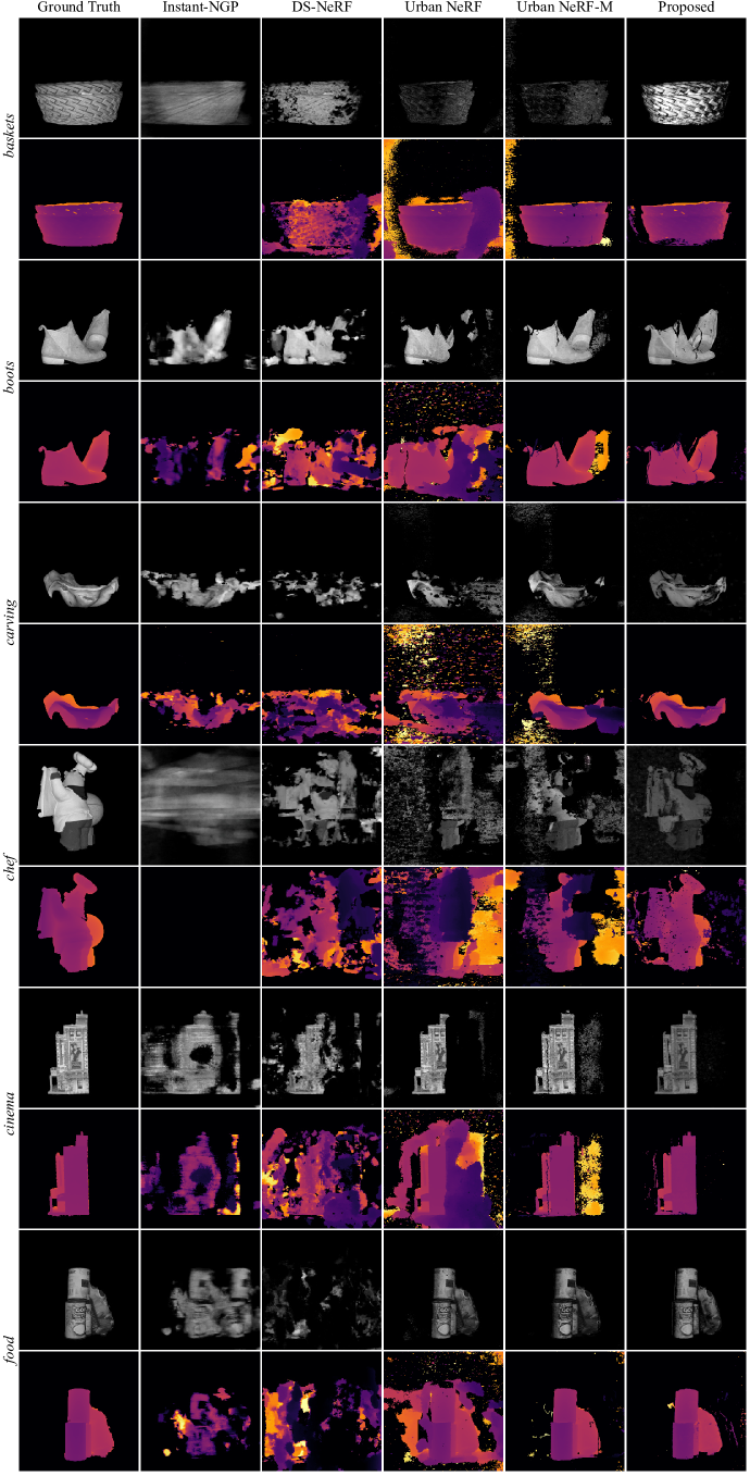
Figure 6: Rendered images and depths on the captured dataset for 3 views.

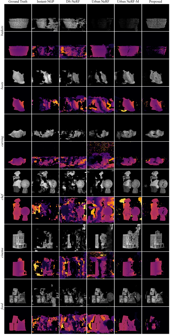
Figure 7: Rendered images and depths on the captured dataset for 5 views.

References

- Rapp et al. [2019] Joshua Rapp, Yanting Ma, Robin MA Dawson, and Vivek K Goyal. Dead time compensation for high-flux ranging. IEEE Trans. Signal Process., 67(13):3471–3486, 2019.
- Grossberg and Nayar [2005] Michael D Grossberg and Shree K Nayar. The raxel imaging model and ray-based calibration. Int. J. Comput. Vis., 61(2):119, 2005.
- Bradski [2000] G. Bradski. The OpenCV Library. Dr. Dobb’s Journal of Software Tools, 2000.
- Paszke et al. [2019] Adam Paszke, Sam Gross, Francisco Massa, Adam Lerer, James Bradbury, Gregory Chanan, Trevor Killeen, Zeming Lin, Natalia Gimelshein, Luca Antiga, Alban Desmaison, Andreas Kopf, Edward Yang, Zachary DeVito, Martin Raison, Alykhan Tejani, Sasank Chilamkurthy, Benoit Steiner, Lu Fang, Junjie Bai, and Soumith Chintala. Pytorch: An imperative style, high-performance deep learning library. In Advances in Neural Information Processing Systems 32, pages 8024–8035. Curran Associates, Inc., 2019. URL http://papers.neurips.cc/paper/9015-pytorch-an-imperative-style-high-performance-deep-learning-library.pdf.
- Liu and Nocedal [1989] Dong C. Liu and Jorge Nocedal. On the limited memory bfgs method for large scale optimization. Math. Program., 45(1-3):503–528, 1989. URL http://dblp.uni-trier.de/db/journals/mp/mp45.html#LiuN89.
- Li et al. [2022] Ruilong Li, Matthew Tancik, and Angjoo Kanazawa. Nerfacc: A general nerf acceleration toolbox. arXiv preprint arXiv:2210.04847, 2022.
- Müller et al. [2022] Thomas Müller, Alex Evans, Christoph Schied, and Alexander Keller. Instant neural graphics primitives with a multiresolution hash encoding. ACM Trans. Graph. (SIGGRAPH), 41(4):1–15, 2022.
- Nimier-David et al. [2019] Merlin Nimier-David, Delio Vicini, Tizian Zeltner, and Wenzel Jakob. Mitsuba 2: A retargetable forward and inverse renderer. ACM Trans. Graph., 38(6):1–17, 2019.
- Deng et al. [2022] Kangle Deng, Andrew Liu, Jun-Yan Zhu, and Deva Ramanan. Depth-supervised NeRF: Fewer views and faster training for free. In Proc. CVPR, 2022.
- Rapp and Goyal [2017] Joshua Rapp and Vivek K Goyal. A few photons among many: Unmixing signal and noise for photon-efficient active imaging. IEEE Trans. Comput. Imaging, 3(3):445–459, 2017.
- Leotta et al. [2019] Matthew J Leotta, Chengjiang Long, Bastien Jacquet, Matthieu Zins, Dan Lipsa, Jie Shan, Bo Xu, Zhixin Li, Xu Zhang, Shih-Fu Chang, et al. Urban semantic 3d reconstruction from multiview satellite imagery. In Proc. CVPR Workshops, 2019.
- Rematas et al. [2022] Konstantinos Rematas, Andrew Liu, Pratul P Srinivasan, Jonathan T Barron, Andrea Tagliasacchi, Thomas Funkhouser, and Vittorio Ferrari. Urban radiance fields. In Proc. CVPR, 2022.
- Royo et al. [2022] Diego Royo, Jorge García, Adolfo Muñoz, and Adrian Jarabo. Non-line-of-sight transient rendering. Computers & Graphics, 107:84–92, 2022.