Self-Compatibility: Evaluating Causal Discovery without Ground Truth

Abstract

As causal ground truth is incredibly rare, causal discovery algorithms are commonly only evaluated on simulated data. This is concerning, given that simulations reflect common preconceptions about generating processes regarding noise distributions, model classes, and more. In this work, we propose a novel method for falsifying the output of a causal discovery algorithm in the absence of ground truth. Our key insight is that while statistical learning seeks stability across subsets of data points, causal learning should seek stability across subsets of variables. Motivated by this insight, our method relies on a notion of compatibility between causal graphs learned on different subsets of variables. We prove that detecting incompatibilities can falsify wrongly inferred causal relations due to violation of assumptions or errors from finite sample effects. Although passing such compatibility tests is only a necessary criterion for good performance, we argue that it provides strong evidence for the causal models whenever compatibility entails strong implications for the joint distribution. We also demonstrate experimentally that detection of incompatibilities can aid in causal model selection.

1 Introduction

Causal relationships are often formalized as directed acyclic graphs (DAGs) (Pearl, 2009), or more general graphical models, which also account for hidden confounders and cycles. Discovering causal relations is an important problem in science, which has led to the development of a diverse range of methods to infer causal graphs from passive observations. These methods are based on various approaches, such as Bayesian priors (Heckerman, 1995), independence testing (Spirtes et al., 2000), additive noise assumptions (Shimizu et al., 2006; Hoyer et al., 2008a), generalizations thereof (Zhang and Hyvärinen, 2009; Strobl et al., 2016), or various implementations of the so-called Independence of Mechanism assumption (Daniusis et al., 2010; Marx and Vreeken, 2017).

Causal discovery algorithms are typically evaluated primarily on simulated data (Lachapelle et al., 2020; Zheng et al., 2020; Ng et al., 2020). This is because causal ground truth is incredibly rare as it often necessitates real-world experiments. These experiments can be not only expensive and potentially unethical, but also frequently infeasible or even ill-defined from the outset (Spirtes and Scheines, 2004). Despite promising performance on simulated data, and in spite of numerous results on the identifiability of causal DAGs or parts thereof from passive observations, skepticism about the applicability of these algorithms on real data is warranted. This is because these algorithms are built on assumptions such as faithfulness, additive noise, post-nonlinear models, or independence principles, all of which can be violated in practice. Indeed, recent studies on causal discovery methods reveal a disconcerting reality about their applicability to real-world datasets (Huang et al., 2021; Reisach et al., 2021). Accordingly, the value of existing algorithms for downstream causal inference tasks is unclear and debated (Imbens, 2020).

In this paper we propose a novel methodology for the falsification of the outputs of causal discovery algorithms on real data without access to causal ground truth. The key idea involves testing the compatibility of the causal models inferred by the algorithm when applied to different subsets of variables. In essence, while statistical learning aims for stability across different subsets of data points, we argue that causal discovery should aim to achieve stability across different subsets of variables. We prove that checking for incompatibilities provides a means of falsifying the outputs of causal discovery, as these incompatibilities indicate either violated causal discovery assumptions or finite sample effects that lead to non-negligible changes in the algorithm’s output.

It is natural to ask if one can trust an algorithm if it satisfies compatibility. To address this question, we align with Popper’s theory of science (Popper, 1959), according to which a hypothesis gathers evidence when numerous attempts to falsify it fail. We argue that, under a sufficiently strong notion of compatibility, the algorithm’s outputs on various subsets of variables entail strong implications for the joint distribution, thereby offering numerous opportunities for falsification.

Our contributions.

In this work we present a novel framework to evaluate causal graphs in the absence of ground truth. Specifically,

• We introduce two different, discrete notions of compatibility: interventional and graphical (Section 2.1). Under these definitions, we prove that if the assumptions of a causal discovery algorithm are met, it’s outputs are compatible in the population limit. Furthermore, we show that all “not too simple” algorithms admit falsification using this approach (Section 2.2).

• We connect compatibility to the causal marginal problem and argue that compatibility entails strong implications for the joint distribution, which can then be falsified statistically. In other words, in the sense of Popper (1959), we show that compatibility offers many possibilities to falsify the outputs of an algorithm (Section 2.3).

• We introduce the self-compatibility score for causal discovery which quantifies the level of incompatibility of the outputs of causal discovery. We argue based on stability arguments from learning-theory that the self-compatibility score can potentially serve as a proxy for measures like Structural Hamming distance (SHD) which require access to ground truth (Section 3).

• We demonstrate the efficacy of our scores for model selection in simulation studies and on real-world data where ground truth knowledge is available. Our results show a significant correlation between self-compatibility score and SHD (Section 4).

1.1 Motivational example

(a) Incompatible DAGs over $S$ and $T$

(b) Joint DAG over $S\cup T$ where the DAGs over $S$ and $T$ are compatible.

Figure 1: Each marginal causal models over $S$ and $T$ implies graphical compatibility constraints for the edge $X-Y$ as the edge can only be directed in one way.

To illustrate our key ideas, we describe a simple example where a causal discovery algorithm results in causal graphs which are incompatible in the sense that they do not admit an acyclic causal graph on the union of nodes. Consider the directed acyclic graph (DAG) in figure 1(b). Assume we are given the two subsets $S=\{X,Y,Z_{1}\}$ and $T=\{X,Y,Z_{2}\}$. We will call a causal model that represents only a subset of all relevant variables a marginal causal model in analogy to the marginal distribution. Assume the PC algorithm (Spirtes et al., 2000; Kalisch and Bühlman, 2007) is applied to samples from the marginal distributions over $S$ and $T$. Suppose the observed distribution violates faithfulness (Spirtes et al., 2000) by satisfying $Y\mathchoice{\mathrel{\hbox to0.0pt{$\displaystyle\perp$\hss}\mkern 2.0mu{\displaystyle\perp}}}{\mathrel{\hbox to0.0pt{$\textstyle\perp$\hss}\mkern 2.0mu{\textstyle\perp}}}{\mathrel{\hbox to0.0pt{$\scriptstyle\perp$\hss}\mkern 2.0mu{\scriptstyle\perp}}}{\mathrel{\hbox to0.0pt{$\scriptscriptstyle\perp$\hss}\mkern 2.0mu{\scriptscriptstyle\perp}}}Z_{2}$ but otherwise only (conditional) independences hold that are required by the Markov condition. PC then outputs the two DAGs in figure 1(a), which entail the interventional statements: $p(y|do(x))=p(y|x)$ (for $S$) versus $p(y|do(x))=p(y)$ (for $T$). This is a contradiction unless $Y\mathchoice{\mathrel{\hbox to0.0pt{$\displaystyle\perp$\hss}\mkern 2.0mu{\displaystyle\perp}}}{\mathrel{\hbox to0.0pt{$\textstyle\perp$\hss}\mkern 2.0mu{\textstyle\perp}}}{\mathrel{\hbox to0.0pt{$\scriptstyle\perp$\hss}\mkern 2.0mu{\scriptstyle\perp}}}{\mathrel{\hbox to0.0pt{$\scriptscriptstyle\perp$\hss}\mkern 2.0mu{\scriptscriptstyle\perp}}}X$, which would be an additional violation of faithfulness in contradiction to our assumption. Hence, the outputs of PC cannot both be correct given the observed joint distribution. Perhaps more strikingly, the marginal models in figure 1(a) have different orientations for the edge between $X$ and $Y$. Accordingly, section 2.1 defines an interventional and a graphical notion of compatibility. Note, that an ordinary statistical cross-validation would not have discovered this inconsistency since we assumed $Y\mathchoice{\mathrel{\hbox to0.0pt{$\displaystyle\perp$\hss}\mkern 2.0mu{\displaystyle\perp}}}{\mathrel{\hbox to0.0pt{$\textstyle\perp$\hss}\mkern 2.0mu{\textstyle\perp}}}{\mathrel{\hbox to0.0pt{$\scriptstyle\perp$\hss}\mkern 2.0mu{\scriptstyle\perp}}}{\mathrel{\hbox to0.0pt{$\scriptscriptstyle\perp$\hss}\mkern 2.0mu{\scriptscriptstyle\perp}}}Z_{2}$ to hold in the population case, rather than assuming that a statistical test accepted independence due to a type II error.

2 Compatibility of causal graphs

Notation. Throughout this paper we will use $[n]:=\{1,\dots,n\}$ for $n\in{\mathbb{N}}$, and for $i\in[n]$ we denote random variables with $X_{i}$, values of a variable with the respective lower case letter $x_{i}$ and their domain with calligraphic letter ${\cal X}_{i}$. By slight abuse of notation we denote a vector of random variables in a set $S$ by $X_{S}$ and a vector of values of these variables with $x_{S}$ and the domain of the vector as ${\cal X}_{S}$, when the order does not matter for our purposes. We denote a vector of $k\in{\mathbb{N}}$ values of single variable with ${\bf x}^{k}_{i}$ and the matrix containing values of all variables in a set $S$ with ${\bf X}^{k}_{S}$. When $k$ does not matter we often omit it. ${\bf X}$ denotes the matrix containing vectors of values for all variables $X_{i}$ for $i\in[n]$. For a probability distribution $P$ over a set of variables $V$ and $S\subset V$ we denote with $P_{S}$ the marginal distribution over $S$ and $p$ be the probability density function of $P$ where we assume for simplicity that there always exists a density with respect to a product measure.

Causal models. Although our proposed compatibility-based evaluation is in principle not restricted to any kind of causal model, we will focus our exposition on graphical models. Precisely, we will use directed acyclic graphs (DAGs) (Spirtes et al., 1999; Pearl, 2009), completed partially directed acyclic graphs (CPDAGs), acyclic directed mixed graphs (ADMGs) (Richardson, 2003; Evans and Richardson, 2014), maximal ancestral graphs (MAGs) and partial ancestral graphs (PAGs) (Zhang, 2008). In the main paper we focus on ADMGs and DAGs. Formal definitions of the remaining graphical models and of the causal semantics of graphical models can be found in section A.1.

Definition 1 (DAG and ADMG)

A mixed graph $G$ consists of a set of nodes $V$ and a set of directed edges $E\subseteq V\times V$ and a set of bidirected edges $B\subseteq\{\{X_{i},X_{j}\}:X_{i},X_{j}\in V\}$. If $(X_{i},X_{j})\in E$ we say there is a directed edge between $X_{i}$ and $X_{j}$ and we write $X_{i}\to X_{j}$. If $\{X_{i},X_{j}\}\in B$ we say there is a bidirected edge and write $X_{i}\leftrightarrow X_{j}$. A mixed graph is called acyclic directed mixed graph (ADMG) if there is no sequence of nodes $X_{0},X_{1},\dots,X_{k},X_{0}$ with $k\in{\mathbb{N}}$ such that there is an edge $X_{i}\to X_{i+1}\in E$ for all $i\in[k]$ and $X_{k}\to X_{0}$. An ADMG with not bidirected edges is called directed acyclic graph (DAG). _□

Definition 2 (causal discovery algorithm)

For the purpose of this paper, a causal discovery algorithm ${\cal A}$ who takes i.i.d. data as input, i.e. a matrix ${\bf X}_{S}$ with $S\subseteq V$ containing samples from $P_{S}$, and whose output is a DAG, CPDAG, ADMG, MAG or PAG over nodes in $S$, denoted by $G_{S}$. _□

Throughout our work, we assume that all data has been generated by a single causal model.

Assumption 1 (existence of joint model)

Whenever we consider $k\in{\mathbb{N}}$ sets of variables $S_{i}$ with $i\in[k]$ and distributions $P_{S_{i}}$ we assume there is set $V$ and a DAG $G=(V,E)$ such that there is a distribution $P_{V}$ where $G$ is the causal graph of $P_{V}$ and for all $i\in[k]$ we have $S_{i}\subseteq V$ and $P_{V}$ has $P_{S_{i}}$ as marginal distributions over $S_{i}$.

Note that the requirement that this data generation is formalized as a DAG is not a hard restriction, as CPDAGs, ADMGs, MAGs and PAGs naturally correspond to DAGs when some variables of the DAG are unobserved (see also section A.1).

2.1 Notions of compatibility: Interventional and Graphical

We now introduce the concept of compatibility between causal graphs. We will discuss later how we can use compatibility of the outputs of a causal discovery algorithm (i.e. the self-compatibility) to falsify these outputs.

Definition 3 (compatibility relative to a joint distribution)

Let ${\cal G}_{V}^{*}$ be the space of tuples of DAGs (CPDAGs, ADMGs, MAGs, PAGs) over subsets of a set $V$. Let ${\cal P}_{V}$ denote the space of probability distributions over $V$. A compatibility notion is a function

$$c:{\cal G}^{*}_{V}\times{\cal P}_{V}\to\{0,1\}.$$

For $k\in{\mathbb{N}}$ and $S_{1},\dots,S_{k}\subseteq V$, the graphs $G_{S_{1}},\dots,G_{S_{k}}$ are called compatible with respect to $c$ and $P_{V}$ if $c(G_{S_{1}},\dots,G_{S_{k}},P_{V})=1$.

_□

In this work we will discuss two compatibility notions. We define a interventional compatibility notion, as we consider it a natural requirement of a causal discovery algorithm to make contradiction-free interventional statements. We also define a graphical notion of compatibility that has the advantage that it does not involve statistical decisions (as it does not depend on the distribution), but it raises conceptual problems that we discuss in section A.3.2.

Definition 4 (interventional compatibility)

Let $k\in{\mathbb{N}}$, $S_{1},\dots,S_{k}$ be sets of variables and $G_{S_{1}},\dots,G_{S_{k}}$ be DAGs (CPDAGs, ADMGs, MAGs, PAGs) and $P$ be a probability distribution over $\cup_{i\in[k]}S_{i}$. Define the interventional compatibility via $c(G_{S_{1}},\dots,G_{S_{k}},P_{V})=1$ iff there exists a set $V\supseteq\cup_{j=1}^{k}S_{j}$, an ADMG $G_{V}$, and a distribution $P_{V}$ where $G_{V}$ is the causal ADMG of $P_{V}$ such that if for $X_{i},X_{j}\in S_{l}$ the intervention $p(x_{j}|do(x_{i}))$ is identifiable (Tian and Pearl, 2002; Perković et al., 2015) in $G_{S_{l}}$, it is identifiable in $G_{V}$ and the probabilities coincide for all identification formulae. _□

The interventional compatibility requires that the different causal graphs do not output different interventional probabilities that cannot possibly come from a joint causal model. The compatibility is with respect to a concrete distribution and does not incorporate any genericity assumptions about $P_{V}$. The second notion of compatibility we discuss in this work is the notion of graphical compatibility. In the main paper we will only define graphical compatibility for ADMGs (and therefore also for DAGs), but in section A.3 we will propose detailed definitions for the other graphical models mentioned in this work.

To define the graphical compatibility, we first discuss what Pearl and Verma (1995) called the latent projection of a graphical model. Precisley, we will define the latent projection of an ADMG like Richardson et al. (2023). We will define the latent projections of other graphical models in section A.3.

Definition 5 (latent ADMG)

Let $G$ be a ADMG with variables $V$ and $S\subset V$. The latent ADMG $L(G,S)$ is the ADMG that contains all nodes in $S$, all edges between nodes in $S$ and additionally

• a directed edge between $X,Y\in S$ if there is a directed path from $X$ to $Y$ where all intermediate nodes are in $V\setminus S$

• a bidirected edge between $X,Y$ if there is a (undirected) path such that every non-endpoint is a collider in $V\setminus S$ and there are arrowheads towards $X$ and $Y$ on the adjacent edges on the path.

_□

By construction, every identification formula in the latent ADMG $L(G,S)$ of a ADMG $G$ is also a valid identification formula in $G$ (see section A.3).

Definition 6 (graphical compatibility of ADMGs)

Let $S_{1},\dots,S_{k}$ be a set of nodes. Then we define graphical compatibility by the function $c$ with $c(G_{S_{1}},\dots,G_{S_{k}})=1$ iff there exists a set $V\supseteq\cup_{j=1}^{k}S_{j}$, and an ADMG $G_{V}$ such that $L(G_{V},S_{j})=G_{S_{j}}$. _□

2.2 Falsifiability of algorithms via compatibility

In this section we demonstrate how compatibility between the outputs of an algorithm on different variables can be used to detect that either the assumptions of the causal discovery algorithm are violated or there are finite sample effects in a way that actually change the output of an algorithm. To this end, we will start to define the terms observational falsifiable and self-compatibility.

Definition 7 (observational falsifiability)

The output of an algorithm ${\cal A}$ is observationally falsifiable with respect to a compatibility notion $c$ if there exists a set of variables $V$, a distribution $P_{V}$ and subsets $S_{1},\dots,S_{k}\subseteq V$ such that for all $\epsilon>0$ there is an $m\in{\mathbb{N}}$ such that

$$c({\cal A}({\bf X}^{m}_{S_{1}}),\dots,{\cal A}({\bf X}^{m}_{S_{k}}),P_{V})=0$$ (1)

with probability $1-\epsilon$, where ${\bf X}_{V}^{m}$ (and all submatrices) is drawn from $P_{V}$. We call the left hand side of equation 1 the self-compatibility of ${\cal A}$ w.r.t. $c$, $S_{1},\dots,S_{k}$ and $P_{V}$. _□

To illustrate this definition, recall that in section 1.1 we have constructed a distribution such that the PC algorithm produces interventionally incompatible results on $\{Z_{1},X,Y\}$ and $\{X,Y,Z_{2}\}$ in the limit of infinite data. Therefore the output of PC is observationally falsifiable.

The following result, while not surprising, ensures that there are no incompatibilities in the limit of infinite data if all assumptions are met.

Lemma 1

Let $k\in{\mathbb{N}}$, $S_{1}\dots,S_{k}$ be sets of variables and $P$ be a probability distribution such that $S_{1},\dots,S_{k}$ and $P$ fulfil the assumptions of a causal discovery algorithm ${\cal A}$ in the sense that in the limit of infinite data ${\cal A}({\bf X}_{S_{i}})=L(G,S_{i})$ for $i\in[k]$, where $G$ is the joint graph from 1. Then ${\cal A}({\bf X}_{S_{1}}),\dots,{\cal A}({\bf X}_{S_{k}})$ are interventionally and graphically compatible (w.r.t. to $P$) in the limit of infinite data. _□

All proofs are in section A.2. Most causal discovery algorithms come with theoretical guarantees that their output is correct under some assumptions.

However, we will now show that all causal discovery algorithms that are not “too simple” or “indecisive” can produce incompatible outputs on different sets of variables. To better understand what we mean by simplistic and indecisive, consider an algorithm ${\cal A}$ that orders nodes according to a simple criterion (e.g. starting from variables with lowest entropy ) and output an ADMG containing the complete DAG with respect to that order for directed edges and additionally bidirected edges between all nodes. The outputs of this algorithm on any subset will be graphically compatible, as the marginal models are the latent projection of the models on supersets and also interventionally compatible, as no interventional distribution is identifiable in any of the graphs. We discuss this example further in section A.5.

Definition 8 (non-bivariate causal discovery)

Let $n\in{\mathbb{N}}$, $V$ be a set of variables with $|V|\geq n$, $X_{i},X_{j}\in V$ and $P_{V}$ and $\widetilde{P}_{V}$ be probability distributions over $V$ such that $P_{\{i,j\}}=\widetilde{P}_{\{i,j\}}$. A causal discovery algorithm ${\cal A}$ is non-bivariate if for some $n>2$ there exist $P_{V}$ and $\widetilde{P}_{V}$ such that for every $\epsilon>0$ there exists a $k\in{\mathbb{N}}$ such that

• $p(x_{i}\mid do(x_{j}))$ is identifiable in ${\cal A}({\bf X}^{k})$ and ${\cal A}(\widetilde{\bf X}^{k})$

• there are identification formulae in ${\cal A}({\bf X}^{k})$ and ${\cal A}(\widetilde{\bf X}^{k})$ respectively such that

  $$p^{{\cal A}({\bf X}^{k}}(x_{i}\mid do(x_{j}))\neq\widetilde{p}^{{\cal A}(\widetilde{\bf X}^{k}}(x_{i}\mid do(x_{j}))$$

with probability $1-\epsilon$, where ${\bf X}^{k}$ denotes a data matrix with $k$ samples drawn from $P_{V}$ and $\widetilde{\bf X}^{k}$ contains samples from $\widetilde{P}_{V}$ and $p^{G}(x_{i}\mid do(x_{j})$ denotes the identification formula from $G$ applied to probability distribution $P$. _□

The definition has two aspects: 1) a non-bivariate algorithm must be able to produce an output that allows identification of a causal effect 2) this output does not only depend on bivariate properties of $X_{i}$ and $X_{j}$ but also depends on the distribution of the other nodes. Note, that ordering the nodes by entropy as describe before is not a non-bivariate algorithm. Further note that we did not require the distributions to fulfil the causal discovery assumptions of ${\cal A}$.

The following theorem asserts that for every non-bivariate causal discovery algorithm ${\cal A}$ there is at least one distribution $P$ for which we can detect that $P$ does not fulfil the causal discovery assumptions of ${\cal A}$ by applying ${\cal A}$ to a subset of variables. We observe:

Theorem 1 (non-bivariate algorithms are observationally falsifiable)

If ${\cal A}$ is non-bivariate it is observationally falsifiable with respect to interventional compatibility. _□

The algorithms that we mentioned so far in this paper are non-bivariate and hence falsifiable.

Lemma 2

The algorithms PC, GES (Chickering, 2002), DirectLiNGAM (Shimizu et al., 2011) and RCD (Maeda and Shimizu, 2020b) are falsifiable. _□

Now we have established that the algorithms in lemma 2 indeed have falsifiable outputs, but due to lemma 1 we cannot “accidentally” falsify their output when all of their assumptions are met and in the absence of finite-sample effects.

Remark 1

Note that our approach does not falsify particular causal graphs. Especially, an algorithm ${\cal A}$ may well output the ground truth graph on ${\bf X}$ but we can still find incompatible models on some subset. Due to lemma 1 we know that incompatibility of the outputs indicates that some assumptions are violated or there are errors due to finite sample effects. In this sense we would argue, that we cannot trust the causal discovery algorithm in this case even if ${\cal A}({\bf X})$ happens to be the ground truth graph. _□

2.3 Is self-compatibility a strong condition?

Popper (1959) argues that the more attempts to falsify a hypothesis fail, the stronger the evidence for this hypothesis is. Particularly, if there is only one joint distributions such that the algorithm outputs compatible graphs, we have many opportunities for falsification.

Definition 9 (merging enabling algorithms)

An algorithm ${\cal A}$ is said to enable merging distributions with respect to a notion of compatibility $c$ if for some set of variables $V$ and $k\in{\mathbb{N}}$ there exists sets $S_{1},\dots,S_{k}\subset V$ and distributions $P_{S_{1}},\dots,P_{S_{k}}$ such that there is exactly one joint distribution $P_{V}$ such that for all $\epsilon>0$ there is a $m\in{\mathbb{N}}$ such that

$$c({\cal A}({\bf X}^{m}_{S_{1}}),\dots,{\cal A}({\bf X}^{m}_{S_{k}}),{\cal A}({\bf X}^{m}_{V}),P_{V})=1,$$

with probability $1-\epsilon$ although there exists also a second distribution $\tilde{P}_{V}$ whose marginals also coincide with all $P_{S_{j}}$ for $j\in[k]$, where ${\bf X}^{m}_{i}$ is drawn from $P_{S_{i}}$ for $i\in[k]$. _□

In other words, the condition of compatibility of causal models implies constraints for the joint distributions that result in a unique solution of the causal marginal problem, although the probabilistic marginal problem (Vorob’ev, 1962) is not unique in this case.

Theorem 2 (FCI enables merging)

The FCI algorithm enables merging w.r.t. graphical compatibility on PAGs. _□

In section A.7 we provide a similar statement for an idealized version of RCD. The proofs construct examples of causal models on $S_{1}:=S\cup\{i\}$ and $S_{2}:=S\cup\{j\}$ for which any compatible joint model on $S_{1}\cup S_{2}$ entails $X_{i}\mathchoice{\mathrel{\hbox to0.0pt{$\displaystyle\perp$\hss}\mkern 2.0mu{\displaystyle\perp}}}{\mathrel{\hbox to0.0pt{$\textstyle\perp$\hss}\mkern 2.0mu{\textstyle\perp}}}{\mathrel{\hbox to0.0pt{$\scriptstyle\perp$\hss}\mkern 2.0mu{\scriptstyle\perp}}}{\mathrel{\hbox to0.0pt{$\scriptscriptstyle\perp$\hss}\mkern 2.0mu{\scriptscriptstyle\perp}}}X_{j}\,|X_{S}$.

Relationship to interventions. Note that there is a close relationship between enabling merging and being able to predict the impact of interventions: assume the node $i$ describes a coin flip triggering the intervention $do(X_{k}=x_{k})$ on node $k\in S$ for $X_{i}=1$. When ${\cal A}$ infers $P_{\{i,j\}}$ after being applied to $S\cup\{i\}$ and $S\cup\{j\}$, it implicitly provides an interventional probability via $p(x_{j}|do(x_{k}))=p(x_{j}|x_{i}=1)$ for an observer who knows that $i$ randomly controls the intervention on $k$.

3 Self-compatibility score

In this section we propose a practical score, that quantifies “how compatible” the outputs of an algorithm applied to different subsets of variables are. This score can be seen as a continuous relaxation of the binary notion of compatibility in definition 3. We propose to use this relaxation, as we showed in theorem 2, self-compatibility is a strong criterion and in practise it is often violated. This score is defined such that a perfect score indicates self-compatibility and in this sense the score can be used to falsify the outputs of a causal discover algorithm as we described before. But moreover, our experimental results in section 4 suggest that the continuous score could be used to evaluate causal discovery algorithms in the sense that it could be used as a “proxy” for the structural Hamming distance, which cannot be evaluated without ground truth knowledge.

The score in this section based on the interventional compatibility notion (definition 4). We give a more detailed explanation in section A.9 and also present a self-compatibility score based on graphical compatibility there. We use the test from Su and Henckel (2022) to test whether the interventional distributions agree.

Definition 10 (interventional self-compatibility score)

Denote the test proposed by Su and Henckel (2022) applied to the distribution $P(Y\mid do(X))$ and the parent-adjustment sets according to causal graphs $G_{1},\dots,G_{k}$ with $T[X,Y;G_{1},\dots,G_{k}]$ with $k\in{\mathbb{N}}$. Let further $S_{1},\dots,S_{k}\subseteq V$. We define the interventional self-compatibility score $\kappa^{I}$ of ${\cal A}$ via

$$\kappa^{I}({\cal A},{\bf X}):=\frac{1}{|V|^{2}-|V|}\sum_{\begin{subarray}{c}X,Y\in V\\ X\neq Y\end{subarray}}\mathbb{I}\left[T\left(X,Y;{\cal A}({\bf X}),{\cal A}({\bf X}_{S_{1}}),\dots,{\cal A}({\bf X}_{S_{k}})\right)\text{ rejects }H_{0}\right],$$ (2)

where $\mathbb{I}[\cdotp]$ denotes the indicator function and $H_{0}$ is the hypothesis that all interventional distributions are the same. Note, that we also always include the result of the causal discovery algorithm on all variables ${\cal A}({\bf X})$. _□

Relationship to stability. While, as previously discussed, it is not possible to guarantee that a causal discovery algorithm that achieves a high self-compatibility score will accurately predict system behavior under interventions, we argue that the resulting models are at least useful due to their ability to predict statistical properties of unobserved joint distributions. This perspective is influenced by Janzing (2018), which reconceptualizes causal discovery as a statistical learning problem. The key principle underlying this reconceptualization posits that causal models offer predictive value beyond predicting system behavior under interventions; they can also predict statistical properties of unobserved joint distributions. See A.6 for the formal setup and description of this idea and the associated learning problem.

Observe that, for a causal discovery method to achieve a high self-compatibility score, it’s output must remain largely unchanged under small modifications to the variable sets it is applied to. Following this idea, in section A.6 we define a notion of stability of a causal discovery algorithm. Under this definition, we provide high-probability generalization bounds for causal models generated by stable causal discovery methods. The result demonstrates that stable algorithms, provably, generate useful causal models due to their ability to generalize statistical predictions across variable sets. Informally, it provides evidence that a high self-compatibility constitutes a useful inductive bias for causal discovery. This is notably distinct from the standard setting in statistical learning, where algorithms that exhibit stability under small modifications to the data are known to generalize across data points.

4 Experiments

We now explore the efficacy of the method described in section 2 on real and simulated data. The details of the experiments can be found in section A.11 and additional experiments in section A.12.

Model evaluation via self-compatibility. As a first experiment focus on a setting where we would expect a causal discovery algorithm to work reasonably well and want to see whether the self-compatibility $\kappa^{I}$, defined in definition 10 indicates many incompatible models in scenarios. We therefore generate 100 datasets (as described in section A.11) with a linear uniform model and ran the RCD algorithm that does not assume causal sufficiency. The left plot in figure 2 shows that interventional compatibility indeed is a strong condition, in the sense that even in this scenario we find many interventionally incompatible marginal graphs. The right hand side of figure 7 shows a strong correlation between $\kappa^{I}$ and the structural Hamming distance of the joint graph to the true graph. We suspected the density of the ground truth graph to influence both, the self-compatibility score as well as the SHD. We therefore also report the partial correlation between SHD and $\kappa^{I}$ given the average node degree of the ground truth graph, which is $-0.45$. This suggests that $\kappa^{I}$ might be a useful proxy for SHD, which we cannot calculate in the absence of ground truth.

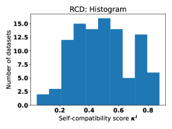
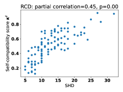
Figure 2: RCD on datasets that fulfill the LiNGAM assumption. Upper: A histogram of $\kappa^{I}$ scores shows that on few datasets RCD is perfectly self-compatible Lower: The structural Hamming distance of estimated graphs $\hat{G}$ to the respective true graph $G$ versus the interventional self-compatibility score $\kappa^{I}$. The self-compatibility score is highly correlated with the SHD. As both are influenced by the degree of the true graph, we also report the partial correlation given the average node degree of the true graph.

Model selection via self-compatibility. As we have seen that the self-compatibility score is correlated with the SHD of the joint model to the ground truth, we now want to investigate whether the score can be used to guide model selection and parameter tuning. We used PC and GES for causal discovery, as these methods both output CPDAGs and therefore their results are comparable.

For each ground truth graph we ranked the algorithms by their graphical self-compatibility score $\kappa^{G}$ (defined in section A.3). More precisely, the winners are defined as $\operatorname{Winner}=\arg\max_{{\cal A}\in\{\operatorname{PC},\operatorname{GES}\}}\kappa^{G}({\cal A},{\bf X})$. where ${\bf X}$ is the full data matrix of each dataset. We then compare the SHD of the joint models found by the two algorithms, i.e. $\operatorname{PC}({\bf X})$ and $\operatorname{GES}({\bf X})$ in terms of their SHD to the ground truth graph. In figure 3 we plot the SHD between the ground truth graph and $\operatorname{Winner}({\bf X})$ on the $x$-axis and the SHD of the result of the respective other algorithm on the $y$-axis. If the self-compatibility score was a “perfect” selection criterion we would hope to see all points on or above the diagonal. In fact, 71% of the points are on or above the line. Moreover, in the right diagram of figure 3 we can see, that in most cases where the self-compatibility score picked the algorithm that produces a worse SHD, the scores of the algorithms were close to each other. In section A.12 we provide additional experiments. Particularly, we will also consider the selection of hyperparameters.

Real data. Finally, we also used self-compatibility on the biological dataset presented in (Sachs et al., 2005) and on the climate dataset from Huang et al. (2021). Wit these experiments we want to illustrate how self-compatibility could be used in practise. We noted that all causal discovery algorithms that we tried performed quite poorly on these datasets. Our self-compatibility score reflects this in the sense that in six out of eight cases we get comparably low self-compatibility score. The two cases where the self-compatibility score was high, were the ones with the best results in terms of SHD and $F_{1}$ score of all real-world experiments. More details can be found in table 1.

5 Related work

To the best of our knowledge we are the first to leverage compatibility constraints of marginal causal models to falsify the output of causal discovery algorithms.

Robustness of causal effects. While we proposed a method to falsify the underlying assumptions of causal discovery algorithms, there exists several methods for scenarios where causal directions are given and the goal is to estimate the strength of the treatment effect. E.g. Walter and Tiemeier (2009); Lu and White (2014); Oster (2019) propose to test whether a regression model is causal by dropping parts of the potential covariates and testing robustness. Similarly, Su and Henckel (2022) present the aforementioned parametric test for the case where a causal graph is given.

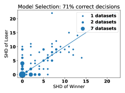
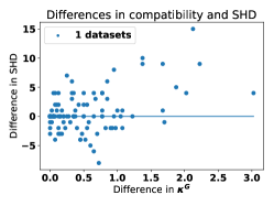
Figure 3: We chose between the algorithms PC and GES according to the self-compatibility $\kappa^{G}$ for 100 datasets. The size of the dots indicates when multiple datasets overlap in the plot. Upper: The SHD of the winner and loser algorithms. As 71% of datasets lie above or on the diagonal, we mostly picked the better model. Lower: The difference in SHD versus the difference in self-compatibility $\kappa^{G}$ between winners and losers. In most cases where we picked the worse model in terms of SHD the difference in $\kappa^{G}$ is small.

Evaluating causal models. The gold standard of evaluating the quality of a causal model would be to conduct a randomized control trial. In contrast, our method allows for falsification in settings where experiments are infeasible. There are other methods to judge the quality of causal models that do not rely on ground truth data as well, but they are limited to special cases, such as falsification via Verma-constraints (Verma and Pearl, 2022) for instrument variables, tests that require parametric assumptions (Bollen and Ting, 1993; Daley et al., 2022) or the derivation of Bayesian uncertainty estimates (Claassen and Heskes, 2012). A common approach is to count the number of $d$-separation statements that are not reflected in the data Textor et al. (2017); Reynolds et al. (2022), although this either requires ground truth again or is also subject to assumptions such as faithfulness. Eulig et al. (2023) propose to reject causal graphs that do not reflect the conditional independences in the data significantly better than a random baseline graph.

Causal marginal problem. Tsamardinos et al. (2012) use causal models on $S_{1},S_{2}$ variables to predict conditional (in)dependences in $P_{S_{1}\cup S_{2}}$. For the toy scenario of a collider structure with three binaries, Gresele et al. (2022) studied compatibility of structural equations for the bivariate marginals, which amounts to falsifiability of causal statements of rung 3 in Pearl’s ladder of causation (Pearl and Mackenzie, 2018). In a scenario where causal directions are known, Guo et al. (2023) define out-of-variable generalization as the capability of a machine learning algorithm to perform well across environments with different causal features, and use marginal observations to predict joint distributions. Janzing (2018) infers a DAG $G$ on $S:=\cup_{j}S_{j}$ in order to predict properties of $P_{S}$ from the set of all $P_{S_{j}}$, which admits falsifying the DAG without interventions via ‘test marginal distributions’ $P_{S_{j+1}}$. Despite the connections discussed in section 2.3, the key difference of these approaches to our method is, that we do not use marginal distributions to learn a joint graph. Instead, we propose to falsify the output of algorithms by learning marginal models.

6 Conclusion

We have proposed a novel method to falsify the output of causal discovery algorithms which does not rely on causal ground truth. It is based on compatibility of the output of an algorithm on different sets of variables. While this compatibility seems, at first glance, just as a weak sanity check, that is, a weak necessary condition for providing good causal models, we have argued that there are cases where the compatibility requirement results in strong predictions for the joint distribution of variables which can be falsified from passive observations (and thus provide strong evidence in favor of causal models if all attempts of falsification fail).

This approach is limited as we can only falsify the outputs of causal discovery. Even though we argue in section 4 that our self-compatibility score could be used as a proxy for SHD, we have no hard theoretical guarantees that ensure good performance for good self-compatibility scores (and we do not think that such guarantees can be proven without further assumptions). Further, our work provides no guidance as to which self-compatibility is “good enough” or when the outputs of an algorithm should definitely be rejected. We leave this to future work.

Appendix A Appendix

With our formalism we mainly follow [Peters et al., 2017, Pearl, 2009].

A.1 Formal definitions

Structural causal models

Causality can be formalized mathematically by saying that all relationships between variables are governed by some deterministic functions except for some genuine, independent sources of randomness.

Definition 11 (structural causal model)

Let $n\in{\mathbb{N}}$ and $V$ be a set of random variables $X_{1},\dots,X_{n}$, $U$ be the a set of variables $N_{1},\dots,N_{n}$ and $P_{U}$ be a probability distribution over $N_{1},\dots,N_{n}$ such that all $N_{1},\dots,N_{n}$ are jointly independent. Let there be a set of (measurable) functions $F$ such that for all $i\in[n]$ we have

$$X_{i}:=f_{i}(PA_{i},N_{i}),$$

where $PA_{i}$ is some subset of $V\setminus\{X_{i}\}$ such that there are no cyclic dependencies between variables and $f_{i}$ depends on all variables in $PA_{i}$. Then we call $(V,U,F,P_{U})$ a structural causal model (SCM). _□

Due to the acyclicity, the distribution $P_{U}$ also entails a unique joint distribution over $V$, as each value $x_{i}$ can be solved recursively until it only depends on noise terms.

Definition 12 (intervention)

Let $\mathcal{S}=(V,U,F,P_{U})$ be an SCM. The intervention $do(X_{i}=x_{i}^{*})$ for some $i\in[n]$ is defined by inserting the fixed value $x_{i}^{*}$ in all equations in $F$ that depend on $X_{i}$, regardless of other variables in the model. Denote with $\mathcal{S}_{do(X_{i}=x_{i})}$ the modified model with these equations. The interventional distribution is defined as the distribution that canonically arises from $\mathcal{S}_{do(X_{i}=x_{i})}$ and we denote it with $P(X_{S}=x_{S}\mid do(X_{i}=x_{i}))$ for any $S\subseteq V$. _□

Graphical models

Often, we do not directly deal with structural causal models, but represent the causal structure graphically. We will first define the graphical structures and then discuss their connection to the causal semantics defined via SCMs. There are several popular graphical models for causality. We mostly follow Zhang [2008], Perković et al. [2015] with out formalism. First recall the definitions of DAGs, mixed graphs and ADMGs from definition 1. We say there is an arrowhead towards $X_{j}$ if there is an edge $X_{j}\to X_{i}\in E$ or $X_{i}\leftarrow X_{j}\in B$ and a tail towards $X_{j}$ if there is an edge $X_{i}\leftarrow X_{j}\in E$. We further say $X_{i}$ and $X_{j}$ are adjacent if $X_{i}\to X_{j}\in E,X_{j}\to X_{i}\in E$ or $X_{i}\leftrightarrow X_{j}\in B$.

Definition 13 (maximal ancestral graphs)

An undirected path is a sequence of nodes $X_{0},\dots,X_{k}$ with $k\in{\mathbb{N}}$ such that either $X_{i}\to X_{i+1}\in E$, $X_{i+1}\to X_{i}\in E$ or $X_{i}\leftrightarrow X_{j}\in B$ for $i\in[k-1]$. A node $X_{i}$ is called collider on an undirected path $p$ if there are two edges with a head towards $X_{i}$ on $p$. We say there is an almost directed cycle if there is a directed cycle from $X_{i}$ to $X_{j}$ and there is a bidirected edge $X_{i}\leftrightarrow X_{j}$. Let $L\subset V$ and call the first and the last nodes on a path the endpoints of a path. An inducing path relative to $L$ is an undirected path $p$, such that every node on $p$ that is in $V\setminus L$ except for the endpoints, is a collider on $p$ and an ancestor of one of the endpoints. A mixed graph $G$ is called a maximal ancestral graph (MAG) if it contains no almost directed cycles and there is no inducing path between non-adjacent nodes. _□

Definition 14 ($m$-separation)

Let $G=(V,E,B)$ be a mixed graph. An undirected path $p$ between $X_{i}$ and $X_{j}$ in $G$ is called $m$-connected given a set $Z\subset V\setminus\{X_{i},X_{j}\}$ if every non-collider on $p$ is not in $Z$ and every collider on $p$ is an ancestor of a node (or is itself) in $Z$. If no undirected path between $X_{i}$ and $X_{j}$ is $m$-connected given $Z$ we say $X_{i}$ and $X_{j}$ are $m$-separated by $Z$ and write $X_{i}\perp_{G}X_{j}\mid Z$. If $G$ is a DAG we also say $d$-separation instead of $m$-separation. _□

Graphical models and causality

Definition 15 (causal DAG)

Let $P$ be a probability distribution over variables in $V$ that has been generated by an SCM $S$ as described above. We call a DAG $G$ a causal graph of $P$ if $G$ contains a node for each variable in $V$ and an edge from $X_{i}$ to $X_{j}\in V$ iff $X_{i}\in PA_{j}$ in $S$. _□

Definition 16 (Global Markov condition)

We say a probability distribution $P$ over $V$ fulfils the global Markov condition w.r.t. the DAG (MAG) $G$ if for every two nodes $X_{i},X_{j}\in V$ and set $Z\subseteq V\setminus\{X_{i},X_{j}\}$ we have that $X_{i}\perp_{G}X_{j}\mid Z$ implies $X_{i}\mathchoice{\mathrel{\hbox to0.0pt{$\displaystyle\perp$\hss}\mkern 2.0mu{\displaystyle\perp}}}{\mathrel{\hbox to0.0pt{$\textstyle\perp$\hss}\mkern 2.0mu{\textstyle\perp}}}{\mathrel{\hbox to0.0pt{$\scriptstyle\perp$\hss}\mkern 2.0mu{\scriptstyle\perp}}}{\mathrel{\hbox to0.0pt{$\scriptscriptstyle\perp$\hss}\mkern 2.0mu{\scriptscriptstyle\perp}}}X_{j}\mid Z$. We also say $P$ is Markovian w.r.t. $G$. If $X_{i}\mathchoice{\mathrel{\hbox to0.0pt{$\displaystyle\perp$\hss}\mkern 2.0mu{\displaystyle\perp}}}{\mathrel{\hbox to0.0pt{$\textstyle\perp$\hss}\mkern 2.0mu{\textstyle\perp}}}{\mathrel{\hbox to0.0pt{$\scriptstyle\perp$\hss}\mkern 2.0mu{\scriptstyle\perp}}}{\mathrel{\hbox to0.0pt{$\scriptscriptstyle\perp$\hss}\mkern 2.0mu{\scriptscriptstyle\perp}}}X_{j}\mid Z$ also implies $X_{i}\perp_{G}X_{j}\mid Z$ we say $P$ is faithful to $G$. _□

A distribution that has been generated by an SCM is always Markovian w.r.t. its causal DAG.

Definition 17 (Markov equivalence)

Two DAGs (MAGs) $G_{1},G_{2}$ are Markov equivalent if for all nodes $X_{i},X_{j}\in V$ and sets of nodes $Z\subseteq V\setminus\{X_{i},X_{j}\}$ we have $X_{i}\perp_{G_{1}}X_{j}\mid Z$ iff $X_{i}\perp_{G_{2}}X_{j}\mid Z$. We call

$$[G]:=\{G^{\prime}:G\text{ and }G^{\prime}\text{ are Markov equivalent}\}$$

the Markov equivalence class of $G$. _□

Definition 18 (CPDAG)

Let $G$ be a DAG. The completed partially directed graph $C$ of $[G]$ is a mixed graph that contains a directed edge $X_{i}\to X_{j}$ iff this edge exists in all DAGs in $[G]$ and a bidirected edge $X_{i}\leftrightarrow X_{j}$ iff there is a DAG in $[G]$ with the edge $X_{i}\to X_{j}$ and a DAG in $[G]$ with the edge $X_{i}\leftarrow X_{j}$. We call $C$ a causal CPDAG if $G$ is a causal DAG. _□

The partial ancestral graph that we now introduce can also represent the presence of selection bias. In this paper we omit this part of the formalism (similarly to Zhang [2008]).

Definition 19 (PAG)

Let $G$ be a MAG over variables in a set $V$. The partial ancestral graph of $[G]$ is a graph $H=(V,E)$ with a symmetric set of edges $E\subseteq V\times V$ and a map $\operatorname{end}:E\to\{>,-,\circ\}$ such that for $X_{i},X_{j}\in V$

• $(X_{i},X_{j})\in E$ and $(X_{j},X_{i})\in E$ if $X_{i},X_{j}$ are adjacent in any graph in $[G]$

• $\operatorname{end}(X_{i},X_{j})=>$ iff there is an arrowhead from $X_{i}$ to $X_{j}$ in every graph in $[G]$

• $\operatorname{end}(X_{i},X_{j})=>$ iff there is no arrowhead from $X_{i}$ to $X_{j}$ in every graph in $[G]$

• $\operatorname{end}(X_{i},X_{j})=\circ$ else.

$X_{i}$ and $X_{j}$ are called adjacent if $(X_{i},X_{j})\in E$. We say there is a directed edge from $X_{i}$ to $X_{j}$ if $\operatorname{end}(X_{i},X_{j})=>$ and $\operatorname{end}(X_{j},X_{i})=-$ and then define directed paths if there are paths of directed edges. We say there is a possibly directed path from $X_{1}$ to $X_{k}$ if there are nodes $X_{1},\dots,X_{k}$ such that $X_{i}$ is adjacent to $X_{i+1}$ and there is no arrowhead towards $X_{i}$ for $i\in[k-1]$. A node $X_{j}$ is a possible descendant of $X_{i}$ if there is a possibly directed path from $X_{i}$ to $X_{j}$. A node $X_{i}$ is collider on a path if there are two arrowheads towards $X_{i}$ on that path. A collider path is a path, such that every non-endpoint is a collider. A direct edge is also a (trivial) collider path. A definite non-collider on a path is a node $X_{i}$ that has at least one tail towards $X_{i}$ on the path and a definite status path is path such that every node on the path is either a collider or a definite non-collider on this path. _□

Definition 20 (visible edge)

Every edge in a DAG or CPDAG is visible. A directed edge $X_{i}\to X_{j}$ in a MAG (PAG) $G$ is visible if there is a node $X_{k}$ not adjacent to $X_{i}$ and there is a collider path from $X_{k}$ to $X_{i}$ such that every non-endpoint of the path is a parent of $X_{j}$ and the last edge towards $X_{i}$ has an arrowhead at $X_{i}$. _□

Identification

We now want to define what we mean with identifiability. The following definition is from Tian and Pearl [2002].

Definition 21 (identifiability)

Let $\mathcal{S}$ be a set of SCMs and $S,S^{\prime}\in\mathcal{S}$ be SCMs with the same causal graph. Any quantity of $Q(S)$ is identifiable in $\mathcal{S}$ if $Q(S)=Q(S^{\prime})$ whenever $P_{S}$ coincides with $P_{S^{\prime}}$, where $P_{S}$ denotes the probability distribution entailed by $S$. _□

Often one assumes that the causal graph $G$ is known and then tries to derive the property $Q(S)$ from $G$ and the distribution $P_{S}$. We want to make the distinction between the graphical properties of $G$ and the distribution $P_{S}$ a bit more explicit, as in our self-compatibility framework we deal with estimated graphs that might not correctly represent the underlying data generation. In such a case, the identification formulae derived from such a graph may be incorrect and different identification formulae may even lead to contradicting results for the quantities of interest.

Definition 22 (identification formula)

Let $S$ be an SCM with causal graph $G$ and identifiable quantity $Q(S)$. A identification formula in $G$ is a map $g:{\cal P}\to{\mathbb{R}}$, such that for a probability distribution $P_{S}$ of $S$ we have $g(P)=Q(S)$, where ${\cal P}$ denotes the space of probability distributions. _□

Note that if we have two different graphs $G,G^{\prime}$, we may have identification formulae $g,g^{\prime}$ for $Q$ in $G$ and in $G^{\prime}$ respectively but for a distribution $P$ we get $g(P)\neq g^{\prime}(P)$, as $G$ and $G^{\prime}$ may be different graphs.

Latent projection

In definition 5 we have already defined how to project ADMGs (and therefore also DAGs) to an ADMG that represent only a subset of variables. We will now define similar projections for MAGs, PAGs and CPDAGs. and start be defining a projection of a DAG to a MAG (see also [Zhang, 2008]). We mainly do this to connect MAGs and PAGs to the SCM formalism, although in principle one could also use MAGs instead of ADMGs in definition 6.

Definition 23 (latent MAG)

Let $G$ be a DAG with variables in $V$ and $S\subseteq V$. The latent MAG $L^{\text{MAG}}(G,S)$ is the MAG that contains all nodes in $S$ and and for $X_{i},X_{j}\in S$

• an edge between $X_{i}$ and $X_{j}$ iff there is an inducing path in $G$ between them

• an arrowhead at $X_{i}$ (or $X_{j}$) iff the last edge of the inducing path has an arrowhead at $X_{i}$ ($X_{j}$).

When no confusion with definition 5 can arise, we also just write $L(G,S)$. We call a MAG $M$ a causal MAG if it is the latent projection of a causal DAG $G$. _□

Definition 24 (latent PAG)

Let $H$ be a PAG with variables in $V$, $S\subseteq V$ and $M$ be some MAG in the equivalence class described by $G$. The latent PAG $L^{\text{PAG}}(H,S)$ is the PAG of $[L^{\text{MAG}}(M,S)]$. We call a PAG $H$ a causal PAG if it is the latent projection of a causal MAG. _□

The latent PAG is well-defined, as all MAGs in the same equivalence class also have the same independence statements in $S$ and therefore, these independences are represented by the same PAG.

It is not possible to define a projection operator for CPDAGs without assumptions about the subset $S$, as this model class cannot represent the presence of latent confounders. Nonetheless, we wanted to include them in our framework as popular causal discovery algorithms like PC and GES output CPDAGs. We chose to only define the projection operator for sets $S$ that fulfil the causal sufficiency assumption, i.e. sets that do not contain two nodes $X_{i},X_{j}\in S$ with common ancestor $L\in V\setminus S$ such that any intermediate nodes on paths from $L$ to $X_{i}$ or $X_{j}$ are also in $V\setminus S$.

Definition 25 (latent CPDAG)

Let $G$ be a DAG with variables $V$ and $S\subset V$ be a subset such that the latent ADMG $L(G,S)$ contains no bidirected edges. Then the latent CPDAG $L(G,S)$ is the CPDAG that represents the equivalence class $[L(G,S)]$. _□

Adjustment criteria

The following theorems from the literature provide graphical criteria to identify interventional probabilities. The first one is Theorem 1 in [Tian and Pearl, 2002].

Theorem 3 (parent adjustment in ADMGs)

Let $G$ be a causal ADMG over discrete variables in $V$ and $X_{i},X_{j}\in V$. if there is no bidirected edge connected to $X_{j}$ we have

$$p(x_{i}|do(x_{j}))=\sum_{pa_{i}}p(x_{i}|x_{j},pa_{j})p(pa_{j}).$$

_□

The sum can easily be replaced by an integral for continuous variables with positive densities. Tian and Pearl [2002] also show the more general result in their Theorem 3:

Theorem 4 (generalised identifiability in ADMGs)

Let $G$ be a causal ADMG over discrete variables in $V$ and $X_{i},X_{j}\in V$. The probability $p(x_{i}|do(x_{j}))$ is identifiable iff there is no bidirected path between $X_{j}$ and any of $X_{j}$’s children. _□

For the other graphical models we considered, Perković et al. [2015] provided the following result in their Theorem 3.4.

Theorem 5 (generalised adjustment criterion)

Let $G$ be a causal DAG, CPDAG, MAG or PAG for the probability distribution $P$ over $V$, $X_{i},X_{j}\in V$ and $Z\subseteq V\setminus\{X_{i},X_{j}\}$. Then we have

$$p(x_{i}|do(x_{j}))=\begin{cases}p(x_{i}|x_{j}),\text{ if }Z=\emptyset\\ \int p(x_{i}|x_{j},x_{Z})p(x_{Z})dx_{Z}\text{, else}\end{cases}$$

if and only if

• every possibly directed path in $G$ from $X_{j}$ to $X_{i}$ starts with a visible edge (see definition 20)

• no element in $Z$ is a possible descendant in $G$ of any $W\in V\setminus\{X_{j}\}$ that lies on a possibly directed path from $X_{j}$ to $X_{i}$

• all definite status paths that are not directed are $m$-separated by $Z$.

_□

A.2 Proofs

Proof (For lemma 1)

The graphical compatibility follows directly from definition 6, as $G$ exists by assumption and ${\cal A}({\bf X}_{S_{i}})=L(G,S_{i})$ for $i\in[k]$ and in the population limit. Similarly, the interventional compatibility follows from the fact that the algorithms find the latent projections of $G$. This renders them causal in the sense of theorems 4 and 5 and therefore the interventional probabilities coincide with the ones in $G$ if they are identifiable. _■

Proof (For theorem 1)

Let the set of variables $S$ and the distributions $P,\widetilde{P}$ be like in 8. Let $\tilde{S}$ with $S\cap\tilde{S}=\{i,j\}$ be such that $\tilde{S}\setminus\{X_{i},X_{j}\}$ are variables of the same type as $S\setminus\{X_{i},X_{j}\}$ with canonical one-to-one correspondence but we will assign different distributions to them now: define $P^{\prime}$ to be such that $\widetilde{P}$ is “copied” to $\tilde{S}$, i.e. $X_{i}$ and $X_{j}$ have the same distribution like in $\widetilde{P}$ and all nodes in $\tilde{S}\setminus\{X_{i},X_{j}\}$ have the same distributions as their corresponding node in $S$ has in $\widetilde{P}$. Then define the joint distribution via

$$P({\bf X}_{S\cup\tilde{S}}):=P({\bf X}_{S\setminus\{i,j\}}|X_{i},X_{j})P(X_{i},X_{j})P^{\prime}({\bf X}_{\tilde{S}\setminus\{i,j\}}|X_{i},X_{j}).$$ (3)

One checks easily that its restrictions to $S$ and $\tilde{S}$ coincide with $P({\bf X}_{S})$ and $\widetilde{P}({\bf X}_{S})$, respectively. By construction, the algorithm ${\cal A}$ will result on contradictory statements about the interventional distribution $p(x_{i}|do(x_{j}))$ when applied to ${\bf X}_{S}$, versus when applied to ${\bf X}_{\tilde{S}}$. Thus we have $c({\cal A}({\bf X}_{S}),{\cal A}({\bf X}_{\tilde{S}}),P_{S\cup\tilde{S}})=0$. _■

Figure 4: This modification of figure 1(a) renders the edge $X\to Y$ visible if FCI is applied to $S^{\prime}$.

Proof (For lemma 2)

We will proof the statment separately for the different algorithms. For PC, GES and FCI we explicitly construct a joint distribution such that the algorithms make contradicting interventional statements on different subsets, as our motivating example from section 1.1 almost suffices to show the statement. For DirectLiNGAM and RCD we show an example where two LiNGAM models with different linear coefficient between $X_{i}$ and $X_{j}$ generate the same marginal for $X_{i}$ and $X_{j}$. Therefore the algorithms are non-bivariate and theorem 1 can be applied.

Recall the graph from figure 1(b) and assume that this is the ground truth graph $G$. Also recall that we constructed a distribution that is Markovian and faithful to $G$ except for the additional independence $Y\mathchoice{\mathrel{\hbox to0.0pt{$\displaystyle\perp$\hss}\mkern 2.0mu{\displaystyle\perp}}}{\mathrel{\hbox to0.0pt{$\textstyle\perp$\hss}\mkern 2.0mu{\textstyle\perp}}}{\mathrel{\hbox to0.0pt{$\scriptstyle\perp$\hss}\mkern 2.0mu{\scriptstyle\perp}}}{\mathrel{\hbox to0.0pt{$\scriptscriptstyle\perp$\hss}\mkern 2.0mu{\scriptscriptstyle\perp}}}Z_{2}$. We have already discussed that the PC algorithm will find the graphs in figure 1(a) in the population limit, as these are the only graphs that capture the conditional independences on the the subsets $X,Y,Z_{1}$ and $X,Y,Z_{2}$ under the assumption of no hidden confounder. Similarly, GES will find the same graphs in the limit of infinite data, as a graph that reflects exactly the independences in the distribution will have an optimal score (Proposition 8 [Chickering, 2002]). Denote the graph that PC and GES finds on $S$ with $G_{S}$ and the one over $T$ with $G_{T}$. In these graphs we get $p^{S}(y|do(x))=p(y|x)\neq p(y)=p^{T}(y|do(x))$ where $p^{S}(y|do(x))$ denotes the causal effect derived from $G_{S}$ using the identification formula from theorem 5 and analogously for $T$. The inequality follows since we had $Y\mathchoice{\mathrel{\hbox to0.0pt{$\displaystyle\perp$\hss}\mkern 2.0mu{\displaystyle\perp}}}{\mathrel{\hbox to0.0pt{$\textstyle\perp$\hss}\mkern 2.0mu{\textstyle\perp}}}{\mathrel{\hbox to0.0pt{$\scriptstyle\perp$\hss}\mkern 2.0mu{\scriptstyle\perp}}}{\mathrel{\hbox to0.0pt{$\scriptscriptstyle\perp$\hss}\mkern 2.0mu{\scriptscriptstyle\perp}}}X$ otherwise, in contradiction to the assumption that $Y\mathchoice{\mathrel{\hbox to0.0pt{$\displaystyle\perp$\hss}\mkern 2.0mu{\displaystyle\perp}}}{\mathrel{\hbox to0.0pt{$\textstyle\perp$\hss}\mkern 2.0mu{\textstyle\perp}}}{\mathrel{\hbox to0.0pt{$\scriptstyle\perp$\hss}\mkern 2.0mu{\scriptstyle\perp}}}{\mathrel{\hbox to0.0pt{$\scriptscriptstyle\perp$\hss}\mkern 2.0mu{\scriptscriptstyle\perp}}}Z_{2}$ is the only independence that is not entailed by the true DAG.

For FCI we have to slightly modify the example to render the edge $X\to Y$ visible (and therefore the interventional probability identifiable). To this end, assume we have the graph $G$ shown in figure 4. Assume that as in the case of PC, all independences are given by $d$-separation in $G$ except for the additional independence $Y\mathchoice{\mathrel{\hbox to0.0pt{$\displaystyle\perp$\hss}\mkern 2.0mu{\displaystyle\perp}}}{\mathrel{\hbox to0.0pt{$\textstyle\perp$\hss}\mkern 2.0mu{\textstyle\perp}}}{\mathrel{\hbox to0.0pt{$\scriptstyle\perp$\hss}\mkern 2.0mu{\scriptstyle\perp}}}{\mathrel{\hbox to0.0pt{$\scriptscriptstyle\perp$\hss}\mkern 2.0mu{\scriptscriptstyle\perp}}}Z_{2}$. On the set $S^{\prime}=\{X,Y,Z_{1},Z_{3},Z_{4}\}$ FCI will find all edges between nodes in $S^{\prime}$ that are in $G$ (although it will only partially direct some of them). In this subgraph, the edge $X\to Y$ is visible as $Z_{3}$ (or $Z_{4}$) has an edge towards $X$ but is not adjacent to $X$. Further, there are no non-causal paths between $X$ and $Y$. Then the empty set is a valid adjustment set according to theorem 5. On $T$, FCI will find the marginal model as in figure 1(a) for the same reason as in section 1.1 (with the edges partially directed). Here, the effect from $X$ to $Y$ is also identifiable. Now we get the same interventional probabilities $p^{S^{\prime}}(y|do(x))=p(y|x)\neq p(y)=p^{T}(y|do(x))$, where $S^{\prime}=S\cup\{Z_{3},Z_{4}\}$.

(a) Graph $G_{1}$ with structural coefficient 1 between $X_{1}$ and $X_{2}$.

(b) Graph $G_{2}$ with structural coefficient 2 between $X_{1}$ and $X_{2}$.

Figure 5: Two causal models that fulfil the LiNGAM assumption, have the same marginal over $X_{1}$ and $X_{2}$ and different coefficient from $X_{1}$ to $X_{2}$.

For DirectLiNGAM and RCD we modify an example from Hoyer et al. [2008b]. Precisely, their example V consists of a linear SCM with three nodes defined via

$$X_{3}:=N_{3},\quad X_{1}:=\beta X_{0}+N_{1},\quad X_{2}:=\alpha X_{1}+\gamma X_{0}+N_{2},$$

where $N_{1},N_{2},N_{3}$ are jointly independent non-Gaussian noise variables. Figure 5 shows two such models. Hoyer et al. [2008b] show that there are two models that cannot be distinguished on the marginal over $\{X_{1},X_{2}\}$, one with structural coefficient $\alpha$ and one with $(\alpha\beta+\gamma)/\beta$ between $X_{1}$ and $X_{2}$. For example, we can set $\alpha=\beta=\gamma=1$ and assume all noise variables to have the same distribution with zero mean and unit variance as visualized in figure 5(a) to get a distribution $P$. Analogously, we define another dsitribution $\tilde{P}$ via a model with $\alpha=2,\beta=1,\gamma=-1$ and we require the noise terms to have the same distributions as in the previous model as shown in figure 5(b). The reader may now easily verify, that the marginals over $\{X_{1},X_{2}\}$ of $P$ and $\tilde{P}$ are identical. Further, DirectLiNGAM and RCD will identify these models when all nodes are observed.

In other words, there are two distributions $P,P^{\prime}$ over $X_{1},X_{2},X_{3}$ (generated by the SCMs described above) that have identical marginals over $X_{1},X_{2}$ but LiNGAM results in different interventional probabilities $p(x_{2}|do(x_{1}))\neq p^{\prime}(x_{2}|do(x_{2}))$. Therefore DirectLiNGAM and RCD are non-bivariate and via theorem 1 they are falsifiable. _■

Proof (For theorem 2)

The idea is that we apply FCI to data generated from the DAG in figure 6 on $S\cup\{i\}$ and $S\cup\{j\}$. In the first case, FCI identifies $i\to k$ as a visible edge, that is, $i$ is an unconfounded cause of $k$. Likewise, FCI infers that $k$ is an unconfounded cause of $j$ in the second case. This unconfoundedness excludes a direct link between $i$ and $j$. Consequently, $S$ $m$-separates $i$ and $j$ in every MAG that is compatible with the two visible edges because $S$ also contains no common child of $i$ and $j$. This way, we can construct the entire joint distribution.

Figure 6: PAGs $G_{1}$ and $G_{2}$ over $S\cup\{i\}$ and $S\cup\{j\}$ respectively. The red edges indicate visible edges. The dotted edges visualize that $G_{2}$ does not contain $i$ and therefore the edges from $p_{1}$ and $p_{2}$ go directly into $k$. There cannot be any edge between $i$ and $j$ due to the visible edges between $i$ and $k$ and $k$ and $j$.

Let $S:=\{k,p_{1},p_{2}\}$ be a set of nodes with $i,j\not\in S$. Let $G_{1}$ and $G_{2}$ denote the PAGs given by the asymptotic outputs when FCI is applied to $S\cup\{i\}$ and $S\cup\{j\}$, respectively, where we assume that the distribution is Markovian to the joint PAG in figure 6. Then $G_{1}$ consists of the edges $p_{1}\to i$, $p_{2}\to i$ and $i\to k$, where the latter is a visible edge as e.g. $p_{1}$ has a direct edge to $i$ and is not adjacent to $k$. Likewise, let $G_{2}$ consist of the edges $p_{1}\to j$, $p_{2}\to j$ and $k\to j$ (as the paths over $i$ are inducing paths w.r.t. $S\cup\{j\})$, where the latter is a visible edge. We now conclude that there cannot be a direct link between $i$ and $j$ as follows: $i\to j$ and $i\leftrightarrow j$ would induce confounding between $k$ and $j$, while $j\to i$ would be a directed cycle. We thus obtain $X_{i}\mathchoice{\mathrel{\hbox to0.0pt{$\displaystyle\perp$\hss}\mkern 2.0mu{\displaystyle\perp}}}{\mathrel{\hbox to0.0pt{$\textstyle\perp$\hss}\mkern 2.0mu{\textstyle\perp}}}{\mathrel{\hbox to0.0pt{$\scriptstyle\perp$\hss}\mkern 2.0mu{\scriptstyle\perp}}}{\mathrel{\hbox to0.0pt{$\scriptscriptstyle\perp$\hss}\mkern 2.0mu{\scriptscriptstyle\perp}}}X_{j}\,|X_{S}$, which enables constructing the joint distribution from the two marginals. _■

A.3 Graphical compatibility

A.3.1 Definition

Now we want to define graphical notions for the remaining types of graphical models.

Definition 26 (purely graphical compatibility)

A compatibility notion $c$ is called purely graphical if it does not depend on $P_{V}$, that is, it can also be written as a function

$$c:{\cal G}_{V}^{*}\to\{0,1\}.$$

_□

We will present several purely graphical compatibility notions for different classes of graphical models respectively. In definition 6 we have already defined graphical compatibility for ADMGs. We will now define graphical compatibility for the other graphical models that we considered.

Definition 27 (graphical compatibility of MAGs)

Let $S_{1},\dots,S_{k}$ be a set of nodes and $G_{S_{1}},\dots,G_{S_{k}}$ be MAGs. Then we define graphical compatibility by the function $c$ with $c(G_{S_{1}},\dots,G_{S_{k}})=1$ iff there exists a set $V\supseteq\cup_{j=1}^{k}S_{j}$, and an DAG $G_{V}$ such that $L(G_{V},S_{j})=G_{S_{j}}$, where $L$ is the latent projection from DAGs to MAGs as defined in definition 23. _□

Definition 28 (graphical compatibility of PAGs)

Let $S_{1},\dots,S_{k}$ be a set of nodes and $G_{S_{1}},\dots,G_{S_{k}}$ be PAGs. Then we define graphical compatibility by the function $c$ with $c(G_{S_{1}},\dots,G_{S_{k}})=1$ iff there exists a set $V\supseteq\cup_{j=1}^{k}S_{j}$, and an DAG $G_{V}$ such that $L^{\text{PAG}}(L^{\text{MAG}}(G_{V},V),S_{j})=G_{S_{j}}$, i.e. if $G_{S_{j}}$ represents the conditional independences of the DAG $G_{V}$ over $S_{j}$. _□

Definition 29 (graphical compatibility of CPDAGs)

Let $S_{1},\dots,S_{k}$ be a set of nodes and $G_{S_{1}},\dots,G_{S_{k}}$ be CPDAGs. Then we define graphical compatibility by the function $c$ with $c(G_{S_{1}},\dots,G_{S_{k}})=1$ iff there exists a set $V\supseteq\cup_{j=1}^{k}S_{j}$, and an DAG $G_{V}$ such that $L(G_{V},S_{j})=G_{S_{j}}$, where $L$ is the latent CPDAG as defined in definition 25. _□

A.3.2 Critical discussion of graphical compatibility

Here we show that a purely graphical criterion implicitly relies on a genericity condition which is close to faithfulness in spirit. Consider, the causal model $Y\to Z$ and recall that ADMG compatibility excludes that an additional variable $X$ influences both $Y$ and $Z$. This conclusion can be criticized, depending on the precise interpretation of $Y\to Z$. Assume our interpretation of $Y\to Z$ reads: “$Y$ is an unconfounded cause of $Z$ in the sense that $p(z|do(y))=p(z|y)$”. One can then construct a causal model with the complete DAG on $X,Y,Z$ in which the relation between $X$ and $Z$ is confounded by a hidden variable $W$. In a linear Gaussian model, we can easily tune parameters such that the confounding bias that $W$ induces on $P(Y,Z)$ cancels out with the confounding bias induced by $Z$. This way, we still have $p(z|do(y))=p(z|y)$ despite the confounding paths. Excluding such a non-generic choice of parameters amounts to faithfulness in a DAG with $X,Y,Z,W,F_{Y}$ where $F_{Y}$ controls randomized interventions on $Y$ (the so-called ‘regime-indicator variable’ of Dawid [2021]). In our example, vanishing confounding bias corresponds to

$$F_{Y}\mathchoice{\mathrel{\hbox to0.0pt{$\displaystyle\perp$\hss}\mkern 2.0mu{\displaystyle\perp}}}{\mathrel{\hbox to0.0pt{$\textstyle\perp$\hss}\mkern 2.0mu{\textstyle\perp}}}{\mathrel{\hbox to0.0pt{$\scriptstyle\perp$\hss}\mkern 2.0mu{\scriptstyle\perp}}}{\mathrel{\hbox to0.0pt{$\scriptscriptstyle\perp$\hss}\mkern 2.0mu{\scriptscriptstyle\perp}}}Z\,|Y,$$

without $d$-separation. In other words, the conclusion that $X\to Y$ together with the unconfounded causal relation $Y\to Z$ is incompatible with the complete DAG on $X,Y,Z$ relies on a genericity condition against which one may raise doubts. After all, it is problematic to benchmark causal discovery algorithms via methods that implicitly rely on principles close to faithfulness, if we on the other hand argue that assumptions like faithfulness are often violated. We cannot resolve this counter argument entirely. It may be reassuring, however, that also model classes that do not rely on faithfulness come to the same conclusion, that is, also exclude the direct link from $X$ to $Z$. This will be shown in the proof of Theorem 2.

A.4 Section moved after main deadline

We kept the caption here to keep the numeration consistent with the main paper.

A.5 Why is committing important for falsification?

In definition 8 we required algorithms to be decisive and non-bivariate in a certain sense. With the following lemma we want to show that also the decisiveness is an important aspect. The algorithm that orders nodes according to entropy and draws confounded arrows from each node to the ones with larger entropy comes close to unfalsifiability: if we exclude the case where some nodes have the same entropy and get thus disconnected, it does not admit the identification of any interventional probability. To see the other extreme case, we construct an algorithm that is equally simple, but commits on interventional probabilities in a way that is almost always falsified:

Lemma 3 (DAG via entropy order is almost always falsified)

Let $T:=\{1,2,3\}$ and $P_{\{1,2,3\}}$ be generic in the sense that the entropies of all variables are different. Assume $H(X_{1})<H(X_{2})<H(X_{3})$, without loss of generality, and assume the further genericity condition

$$\sum_{x_{1}}p(x_{3}|x_{2},x_{1})p(x_{1})\neq p(x_{3}|x_{2}).$$ (4)

Then the complete DAGs $G_{\{1,2\}}$ and $G_{\{1,2,3\}}$, obtained by entropy ordering of nodes, are interventionally incompatible. _□

Proof

The left hand side of (4) is $p(x_{3}|do(x_{2}))$ in ${\cal A}(P_{\{1,2,3\}})$, while the right hand side is the same interventional probability in ${\cal A}(P_{\{2,3\}})$.

Note that $P_{T}$ in Lemma 3 is always Markovian with ${\cal A}(P_{\{1,2,3\}})$ because this is a complete DAG. It is thus notable that the algorithm falsifies its own model although $P_{T}$ is a distribution that is allowed by ${\cal A}(P_{\{1,2,3\}})$.

A.6 Relationship to Stability

In this section, we motivate our self-compatibility score using stability arguments from learning theory [Shalev-Shwartz et al., 2010]. Observe that, for a causal discovery method to achieve a high self-compatibility score, it’s output must remain largely unchanged under small modifications to the variable sets it is applied to. Following this idea, under some notion of stability of a causal discovery algorithm, we now show that stable algorithms, provably, generate useful causal models in the sense described below.

While, it is not possible to guarantee that a causal discovery algorithm that achieves a high self-compatibility score will accurately predict system behavior under interventions, we argue that the resulting models are at least useful due to their ability to predict statistical properties of unobserved joint distributions. This perspective is influenced by Janzing [2018], which reconceptualizes causal discovery as a statistical learning problem. The key principle underlying this reconceptualization posits that causal models offer predictive value beyond predicting system behavior under interventions; they can also predict statistical properties of unobserved joint distributions. To illustrate the main idea, consider the following example.

Consider a set of variables $\mathcal{X}=\left\{X_{1},X_{2},\cdots X_{n}\right\}$, and let $\mathcal{S}$ represent a collection of subsets of $\mathcal{X}$. A statistical property $Q$ can be defined as a mapping from $\mathcal{S}$ to $\mathbb{R}$. For a given tuple $S_{i}=(X_{l_{1}},X_{l_{2}},\cdots X_{l_{k}})$, $Q$ might indicate whether the conditional independence $X_{l_{1}}\mathchoice{\mathrel{\hbox to0.0pt{$\displaystyle\perp$\hss}\mkern 2.0mu{\displaystyle\perp}}}{\mathrel{\hbox to0.0pt{$\textstyle\perp$\hss}\mkern 2.0mu{\textstyle\perp}}}{\mathrel{\hbox to0.0pt{$\scriptstyle\perp$\hss}\mkern 2.0mu{\scriptstyle\perp}}}{\mathrel{\hbox to0.0pt{$\scriptscriptstyle\perp$\hss}\mkern 2.0mu{\scriptscriptstyle\perp}}}X_{l_{2}}|X_{l_{3}},\cdots X_{l_{k}}$ holds, represented as $Q(S_{i})=1$ (if true) or $Q(S_{i})=0$ (if false).

Causal models such as Directed Acyclic Graphs (DAGs) can thus be viewed as predictors of statistical properties, like conditional independences. The statistical property predicted by a causal model $\mathcal{M}$ is denoted as $\widehat{Q}_{\mathcal{M}}:\mathcal{S}\rightarrow\mathbb{R}$.

The statistical prediction problem can now be outlined as follows: Given a set of $m$ observations $\mathbb{S}=\left\{S_{1},S_{2},\cdots S_{m})\right\}\in\mathcal{S}^{m}$, and a loss function $l:Q(\mathcal{S})\times Q(\mathcal{S})\rightarrow[0,1]$, the goal of causal discovery is to learn a joint causal model over $\mathcal{X}$ that minimizes the loss $l(\widehat{Q}_{\mathcal{M}}(S),{Q}(S))$ on unobserved subsets $S\in\mathcal{S}$. As an illustrative example, the PC algorithm constructs a joint causal model across all variables—encoding conditional independences for any subset of $\mathcal{X}$—by evaluating conditional independences within a selected set of smaller subsets.

If we assume that the subsets are drawn according to a distribution over $\mathcal{S}$, we can invoke stability arguments from learning theory to guarantee generalization from observed to unobserved sets of variables for causal discovery algorithms that demonstrate stability under small modifications to variable sets. This is notably distinct from the standard setting in statistical learning, where algorithms that exhibit stability under small modifications to the data are known to generalize across data points [Shalev-Shwartz et al., 2010].

In order to formalize our discussion, let’s define the concept of ’stability’ in the context of causal discovery. While there are many related notions of stability in statistical learning theory, their relevance varies depending on the context. In our case, Leave-one-out (LOO) stability [Mukherjee et al., 2006], which requires stability of the loss when a single data point (or a subset of data points) is included or excluded from the training set, is particularly applicable. Nonetheless, to maintain a high-level perspective, we will introduce a strong, distribution-independent form of stability: uniform stability [Bousquet and Elisseeff, 2002], which encompasses other weaker forms of stability like LOO stability.

Definition 30 (Uniform Stability)

A causal discovery algorithm $A$ is said to be $\gamma-$uniformly stable with respect to the loss function $l$ if, for any $S\in\mathcal{S}$, any subset $\mathbb{S}=\left\{S_{1},S_{2},\cdots S_{m}\right\}\subset\mathcal{S}^{m}$, and for any index $i\in[m]$, the following inequality holds:

$$|l(\widehat{Q}_{A_{\mathbb{S}}}(S),{Q}(S))-l(\widehat{Q}_{A_{\mathbb{S}^{/i}}}(S),{Q}(S))|\leq\gamma,$$

where $S^{/i}$ denotes the set $\mathbb{S}$ replacing the element $S_{i}$ by some $S^{\prime}_{i}\in\mathcal{S}$. _□

With this definition, we can formally prove that stable causal discovery algorithms generate useful causal hypotheses in the sense of their ability to generalize statistical predictions across variable sets. To this end, we first introduce the notions of empirical and true risks and state the key result in Theorem 6.

Definition 31 (Empirical and Expected Risks)

Under the reconceptualization of causal discovery as a learning problem, assuming that the subsets are drawn according to a distribution $\mathbb{L}$ over $\mathcal{S}$, the empirical ($\widehat{R}(\mathcal{M})$) and expected risks ($R(\mathcal{M})$) incurred by a causal model $\mathcal{M}$ are defined as:

$$\widehat{R}(\mathcal{M})\coloneqq\frac{1}{n}\sum\limits_{i=1}^{m}l(Q_{\mathcal{M}}(S_{i}),Q(S_{i})),\quad R(\mathcal{M})\coloneqq\mathbb{E}_{\mathbb{L}}[l(Q_{\mathcal{M}}(S_{i}),Q(S_{i}))].$$

_□

Under this definition, one can leverage recent results from Bousquet et al. [2020] to derive the following high probability generalization bounds for uniformly stable causal discovery algorithms.

Theorem 6 (Generalization bounds for uniformly stable causal discovery)

Let $A$ denote a causal discovery algorithm that is $\gamma-$uniformly stable with respect to the loss function $l$ in the sense described above. Then there exists a constant c such that for any probability distribution $\mathbb{L}$ over $\mathcal{S}$ and for any $\delta\in(0,1)$, the following holds with probability at least $1-\delta$ over the draw of $m$ subsets $S_{1},S_{2},\ldots,S_{m}$ according to $\mathbb{L}$:

$$R(A(\mathbb{S}))-\widehat{R}(A(\mathbb{S}))\leq c\Big{(}\gamma\log(n)\log(1/\delta)+\frac{\sqrt{\log(1/\delta)}}{\sqrt{n}}\Big{)},$$

where $A(\mathcal{S})$ denotes the causal model output by the causal discovery algorithm $A$ applied on the set $\mathbb{S}=\left\{S_{1},S_{2},\cdots,S_{m}\right\}$. _□

The result demonstrates that stable algorithms, provably, generate useful causal models due to their ability to generalize statistical predictions across variable sets. Informally, it provides evidence that a high self-compatibility constitutes a useful inductive bias for causal discovery. This is notably distinct from the standard setting in statistical learning, where algorithms that exhibit stability under small modifications to the data are known to generalize across data points.

A.7 Further results about merging

In theorem 2 we have seen that FCI enables what we have called merging in definition 9. We now want to show that an idealized version of RCD also has this property. Repetitive Causal Discovery (RCD) [Maeda and Shimizu, 2020a] is a modification of LiNGAM which is able to also infer latent confounders. It assumes a linear model with independent non-Gaussian noise, where confounding is modelled by some shared noise-variables. Explicitly, it reads:

$$X_{i}=\sum_{j}\beta_{ij}X_{j}+\sum_{j}\epsilon_{ij}W_{j}+N_{i},$$ (5)

where all $N_{i},W_{j}$ are independent noise variables (with non-zero variance). The variables $W_{j}$, which are shared by at least two $X_{i}$, describe the confounding.

Definition 32 (idealized RCD)

We define idealized RCD to be a causal discovery algorithm that has an additional output token, that indicates that idealized RCD ’abstain from a decision’, i.e. it indicates that (idealized RCD estimated that) the distribution cannot be generated via equation 5. Otherwise, it draws an arrow $X_{i}\to X_{j}$ whenever $\beta_{ij}\neq 0$, and a bidirected link whenever they share a variable $W_{k}$, that is, there exists a $k$ such that $\epsilon_{ik}\neq 0$ and $\epsilon_{jk}\neq 0$ according to the usual RCD algorithm.

_□

Theorem 7 (idealized RCD enables merging)

Idealized RCD enables merging with respect to graphical consistency on ADMGs (if the output ’abstain’ is by definition incompatible with all other outputs on subsets). _□

Proof

For the variables $X_{1},X_{2},X_{3}$, assume that idealized RCD outputs $X_{1}\to X_{2}$ (without confounding) asymptotically when applied to data from $P_{\{1,2\}}$. Assume further, that it outputs $X_{2}\to X_{3}$ (without confounding) when applied to data from $P_{\{2,3\}}$. We now show that applying RCD to all three variables can only yield compatible results if $X_{1}\mathchoice{\mathrel{\hbox to0.0pt{$\displaystyle\perp$\hss}\mkern 2.0mu{\displaystyle\perp}}}{\mathrel{\hbox to0.0pt{$\textstyle\perp$\hss}\mkern 2.0mu{\textstyle\perp}}}{\mathrel{\hbox to0.0pt{$\scriptstyle\perp$\hss}\mkern 2.0mu{\scriptstyle\perp}}}{\mathrel{\hbox to0.0pt{$\scriptscriptstyle\perp$\hss}\mkern 2.0mu{\scriptscriptstyle\perp}}}X_{3}\,|X_{2}$ and thus

$$P(X_{1},X_{2},X_{3})=P(X_{1},X_{2})P(X_{3}|X_{2}).$$

Consequently, the joint distribution follows uniquely from the two marginal distributions. The proof builds heavily on the theorem of Darmoir-Skitovic [Darmois, 1953, Skitovic, 1962], which entails that for any set of independent non-Gaussian variables $Y_{1},\dots,Y_{d}$ with non-zero variance, we have

$$\sum_{j}a_{j}Y_{j}\mathchoice{\mathrel{\hbox to0.0pt{$\displaystyle\perp$\hss}\mkern 2.0mu{\displaystyle\perp}}}{\mathrel{\hbox to0.0pt{$\textstyle\perp$\hss}\mkern 2.0mu{\textstyle\perp}}}{\mathrel{\hbox to0.0pt{$\scriptstyle\perp$\hss}\mkern 2.0mu{\scriptstyle\perp}}}{\mathrel{\hbox to0.0pt{$\scriptscriptstyle\perp$\hss}\mkern 2.0mu{\scriptscriptstyle\perp}}}\sum_{j}b_{j}Y_{j}\quad\Rightarrow a_{j}\cdot b_{j}=0\quad\forall j.$$

In other words, two linear combinations can only be independent if they share none of the variables.

If RCD accepts the joint distribution $P_{\{1,2,3\}}$ to be compatible with the two marginal models, it needs to be described by a model of the form (5) with causal ordering $1,2,3$. For different order, causal directions would not be compatible. Further, RCD would abstain from a decision if the joint model was not of the form (5), which we also count as incompatibility. Hence, compatibility entails a joint model of the following form:

$$X_{1} = \sum_{j}\epsilon_{1j}W_{j}+N_{1}$$ (6)

$$X_{2} = \beta_{21}X_{1}+\sum_{2j}\epsilon_{j}W_{j}+N_{2}$$ (7)

$$X_{3} = \beta_{31}X_{1}+\beta_{32}X_{2}+\sum_{j}\epsilon_{3j}W_{j}+N_{3}.$$ (8)

For all $j$ we have $\epsilon_{1j}\epsilon_{2j}=0$ otherwise the causal relation $X_{1}\to X_{2}$ would be confounded and RCD could not output an unconfounded link as bivariate model. This can be seen as follows. RCD only outputs an unconfounded link $X_{1}\to X_{2}$ if $X_{2}-\alpha X_{1}$ is independent of $X_{1}$ for some $\alpha$. This can only be true for $\alpha=\beta_{21}$, otherwise both expressions contain $N_{1}$. Further, $X_{2}-\beta_{21}X_{1}=\sum_{j}\epsilon_{2j}W_{j}+N_{2}$ can only be independent of $\sum_{j}\epsilon_{2j}W_{j}+N_{1}$ if the linear combinations share no $W_{j}$. In a similar way we conclude that $\epsilon_{2j}\epsilon_{3j}=0$: We first check that $X_{3}-\alpha X_{2}$ can only be independent of $X_{2}$ for $\alpha=\beta_{32}$, otherwise $N_{2}$ appears in both expressions. Further, $X_{3}-\beta_{32}X_{2}$ can only be independent if they share none of the variables $W_{j}$.

The variables $W_{j}$ thus fall into three classes: those that appear in only one of the variables $X_{1},X_{2},X_{3}$ and those that are shared by $X_{1}$ and $X_{3}$. The former ones can be absorbed into the noise variables $N_{j}$. We thus simplify (6) to (8) to

$$X_{1} = \sum_{j}\epsilon_{1j}W_{j}+N_{1}$$ (9)

$$X_{2} = \beta_{21}X_{1}+N_{2}$$ (10)

$$X_{3} = \beta_{31}X_{1}+\beta_{32}X_{2}+\sum_{j}\epsilon_{3j}W_{j}+N_{3}.$$ (11)

In a similar way as we have repeatedly argued, $X_{3}-\alpha X_{2}$ can only be independent of $X_{2}$ if $\alpha=\beta_{31}$. We obtain

$$X_{3}-\beta_{32}X_{2} = \beta_{31}\sum_{j}\epsilon_{1j}W_{j}+\sum_{j}\epsilon_{31}W_{j}+\beta_{31}N_{1}+N_{3}.$$ (12)

This expression can only be independent of $X_{1}$ if $\beta_{31}=0$, otherwise $N_{1}$ appears in both expressions. The remaining term $\sum_{j}\epsilon_{31}W_{j}+N_{3}$ can only be independent of $X_{1}$ if there is no $W_{j}$ shared by $X_{1}$ and $X_{2}$, i.e., $\epsilon_{1j}\epsilon_{3j}=0$ for all $j$. However, then the respective linear combination of all $W_{j}$ that appear only in $X_{1}$ can be merged with $N_{1}$, and the others with $N_{3}$. Thus, we end up with the structural equations

$$X_{1} = N_{1}$$ (13)

$$X_{2} = \beta_{21}X_{1}+N_{2}$$ (14)

$$X_{3} = \beta_{32}X_{2}+N_{3},$$ (15)

which implies $X_{1}\mathchoice{\mathrel{\hbox to0.0pt{$\displaystyle\perp$\hss}\mkern 2.0mu{\displaystyle\perp}}}{\mathrel{\hbox to0.0pt{$\textstyle\perp$\hss}\mkern 2.0mu{\textstyle\perp}}}{\mathrel{\hbox to0.0pt{$\scriptstyle\perp$\hss}\mkern 2.0mu{\scriptstyle\perp}}}{\mathrel{\hbox to0.0pt{$\scriptscriptstyle\perp$\hss}\mkern 2.0mu{\scriptscriptstyle\perp}}}X_{3}\,|X_{2}$.

A.8 Section moved after main deadline

We kept the caption here to keep the numeration consistent with the main paper.

A.9 Practical evaluation of compatibility

A.9.1 Details of interventional self-compatibility score

We have already introduced our interventional compatibility score in definition 10. In this section we want to shortly elaborate on this score to avoid confusion.

Su and Henckel [2022] propose to falsify interventional statements of a linear causal model by comparing the interventional distributions entailed by different adjustment sets. More precisely: in many cases a causal DAG $G$ implies several sets $C_{1},\dots,C_{k}$ for $k>2$ satisfying the backdoor criterion Pearl [2009] such that

$$p(y\mid do(x))=\sum_{c_{i}}p(y\mid x,c_{i})p(c_{i}),$$

for all $i\in[k]$. Figure 1(b) is a (rather trivial) example, as we could use $\emptyset$ and $\{Z_{1}\}$. The set of parents of $X$ is always such an adjustment set if the effect is identifiable [Tian and Pearl, 2002]. If $G$ is the true causal model, we can decide whether a set $C$ is a valid adjustment set by graphical criteria (see theorem 5). Su and Henckel [2022] now propose a statistical test to reject the null-hypothesis $H_{0}$ that all sets under consideration yield the same interventional distribution. Precisely, for $C_{1},\dots,C_{k}$ sets of variables the hypothesis reads

$$H_{0}:\quad\beta_{X_{i},X_{j}\cdot C_{1}}=\dots=\beta_{X_{i},X_{j}\cdot C_{k}},$$

where $\beta_{X_{i},X_{j}\cdot C_{l}}$ denotes the partial regression coefficient for $X_{i}$ regressed on $X_{j}$ and all variables in $C_{l}$ for some $l\in[k]$.

We build on their work in the following sense: instead of using one causal model $G$ to derive multiple adjustment sets, we use adjustment sets of different causal models, learned on different subsets of variables. Just as in their work, they should all yield the same interventional distributions. For simplicity, we use parent adjustment for each marginal model. Note, that in the case where all models are correct, each parent-adjustment set in a marginal model will be a valid adjustment set in the joint model. But that the marginal parent sets are valid adjustment sets in the joint model is neither sufficient nor necessary for the test to accept.

A.9.2 Graphical self-compatibility score

The score defined in definition 10 is only applicable to linear models, as we build on the test of Su and Henckel [2022]. As non-linear models are ubiquitous in practise, we also want to propose a score that can be applied in these settings. Graphical compatibility notions do not require any statistical test, thus we chose to build on them for this purpose. Definition 6 always refers to the existence of a joint model. Therefore we found it natural to check the compatibility of each marginal causal graph with the causal graph ${\cal A}({\bf X})$ that an algorithm outputs on all available variables (even though, if we do not assume that the observed variables are causally sufficient, ${\cal A}$ can at most output a latent projection of the joint graph in 1). Further, definition 6 requires that the latent projection to the and the marginal graph are identical. We relax this notion by taking the Structural Hamming Distance (SHD) between the joint model ${\cal A}({\bf X})$ and a marginal model. The SHD is zero iff the graphs are identical.

Definition 33 (graphical self-compatibility score)

Let $k\in{\mathbb{N}}$ and $S_{1},\dots,S_{k}\subseteq V$. We define the graphical self-compatibility score $\kappa^{G}$ of ${\cal A}$ via

$$\kappa^{G}({\cal A},{\bf X}):=\frac{1}{k}\sum_{i\in[k]}\operatorname{SHD}\left(L({\cal A}({\bf X}),S_{i}),{\cal A}({\bf X}_{S_{i}})\right),$$ (16)

where $L$ is the respective projection operator from definitions 5, 25, 23 and 24 for the output of ${\cal A}$.

_□

A.9.3 Further practical considerations

In the following we want to specify some aspects of definitions 10 and 33 that have not been discussed in detail and also slightly modify definition 33 further to tackle some practical issues.

Sampling of subsets. In definitions 10 and 33 we have assumed the subsets are given. In practise, we sample them randomly. But we did not sample from the set of all possible substes for the following reason: if a subset is very small, some algorithms like the PC algorithm often give uninformative outputs in the sense that most edges are unoriented. On the other hand, if subsets are large and differ only by few nodes, the resulting marginal models usually do not differ much. Therefore, in all experiments, we uniformly drew subsets $S_{i}$ from the set of subsets with $|S_{i}|=\lceil|V|/2\rceil$ for $i=1,\dots,l$ for some $l\in{\mathbb{N}}$.

Causal sufficiency. In practise, many algorithms like the PC algorithm or GES rely on the assumption that all causally relevant variables are observed, i.e. that there is no common cause between two observed variables that is itself unobserved and all directed paths from this common cause to the observed nodes only contains unobserved nodes. Clearly, if we sample the subsets uniformly from all subsets with the same size, causal sufficiency will often be violated for these subsets, even if it holds for $V$. Consequently, if we detect an incompatibility between ${\cal A}({\bf X})$ and ${\cal A}({\bf X}_{S})$ we cannot know whether this indicates an actual error or it is simply due to the newly introduced hidden confounder. Still, in section 4 we will show experiments with PC, GES that indicate that self-compatibility might help in model selection for these algorithms. We hypothesise that this is because the self-compatibility scores $\kappa^{G}$ and $\kappa^{I}$ are noisy anyway and that the introduced hidden confounding does on average not change the marginal models too much. And since real data sets almost never contain a causally sufficient set of variables, it seems fair to test algorithms that assume sufficiency nevertheless on subsets with hidden confounding.

CPDAGs and hidden confounders. In definition 25 we have only defined the latent projection of DAG to a CPDAG on causally sufficient subsets. But as we have just discussed, we will not only look at causally sufficient subsets. In the experiments, we simply calculated the latent ADMG and deleted its bidirected edges. The resulting graph is a DAG again and we proceeded with its respective CPDAG.

A.10 Section moved after main deadline

We kept the caption here to keep the numeration consistent with the main paper.

A.11 Experimental Details

A.11.1 Data generation

For our first experiments, we generated synthetic data. We first sampled a random ground truth graph using the Erdos-Renyi model (with number of nodes $n$ and expected degree $d$). For each node $X$ we then define a functional model from the class of linear models. For the linear model we drew the parameters uniformly from $[-1.5,-0.5]\cup[0.5,1.5]$. We then apply an additive noise term which is either drawn from a standard normal distribution or a uniform distribution with zero mean and unit variance.

In all experiments we used graphs with 10 nodes and expected degree 2, as well as linear Gaussian and linear uniform structural equations. For all self-compatibility scores we drew 40 subsets uniformly from the set of all subsets with size 5.

A.11.2 Other details

We evaluated the SHD of CPDAGs and PAGs with respect to the respective CPDAG and PAG of the ground truth graph and for PAGs, according to the definition in [Triantafillou and Tsamardinos, 2016]. For the test of Su and Henckel [2022] in the interventional compatibility score we always chose the confidence level $0.05$. In figures 7, 8 and 3 we chose the parameters $\alpha$ of PC and $\lambda$ of GES via a grid search over $\{0.1,0.01,0.001,0.0001\}$ and $\{10,1,.1,.01,.001\}$ respectively for 10 additional datasets for which we assumed ground truth knowledge, generated analogously to the main datasets. For figure 2 we set all confidence thresholds to $0.1$.

The computations were done on an Intel Core i5-5200U CPU and with 8 GB RAM. All experiments can be run in less than two days.

A.12 Additional experiments

A.12.1 Model evaluation

In section 4 we have already seen that $\kappa^{I}$ is correlated with the SHD to the ground truth graph for RCD on linear non-Gaussian data.

In the next line of experiments we wanted to see whether this correlation also occurs in the setting where algorithms assume causal sufficiency and with the graphical criterion $\kappa^{G}$. We therefore generated 100 datasets (as described above) and estimated graphs $\hat{G}$ with two different causal discovery methods, namely PC and GES.

In figure 7 we see again that this yields a significant partial correlation between the self-compatibility score and SHD. Recall, that we considered the partial correlation given the average node degree of the ground truth graph, as we suspect the density of the ground truth graph to affect both, the SHD and the self-compatibility score.

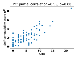
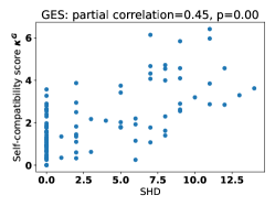
Figure 7: The structural Hamming distance of estimated graphs $\hat{G}$ to the respective true graph $G$ is on the $x$-axis and on the $y$-axis the self-compatibility score $\kappa^{G}$.

A.12.2 Model selection

To check that the results in section 4 do not depend on $\kappa^{G}$, we repeated the experiment with $\kappa^{I}$. Figure 8 shows a similarly good performance, as we chose the correct model in 74% of datasets.

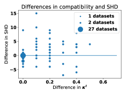
Figure 8: We used the self-compatibility score $\kappa^{I}$ for model selection between PC and GES analogously to the main paper. We picked the model with the better $\kappa^{I}$ score as winner and report the SHD of the winner and of the loser on $x$-axis and $y$-axis respectively. The dot size indicates that several points overlap.

The PC algorithm has exactly one hyperparameter, namely the threshold $\alpha$ below which a p-values of the conditional independence test leads to a rejection of the null hypothesis. We repeated an analogous experiment as above with the PC algorithm with several different $\alpha$ values. We considered multiple runs of PC with different $\alpha$-levels as different causal discovery algorithms in the sense of the previous experiment, i.e. if we denote the PC algorithm that uses $\alpha$ as threshold with $\operatorname{PC}^{\alpha}$, we pick winners via

$$\operatorname{Winner}=\arg\max_{{\cal A}\in\{\operatorname{PC}^{\alpha_{1}},\operatorname{PC}^{\alpha_{2}},\operatorname{PC}^{\alpha_{3}},\operatorname{PC}^{\alpha_{4}}\}}\kappa^{G}({\cal A},{\bf X})$$

with $\alpha_{1}=0.1,\alpha_{2}=0.01,\alpha_{3}=0.01$ and $\alpha_{4}=0.001$ and losers analogously with the minimum. The plots in figure 9 suggest that again, the self-compatibility score is an effective selection criterion and here we even make correct decisions 81% of the cases.

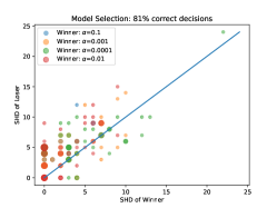
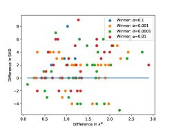
Figure 9: We used the self-compatibility score $\kappa^{G}$ for model selection of the PC algorithm with different $\alpha$ thresholds.

Similarly, we used the interventional self-compatibility score to select hyperparameters for the RCD algorithm. RCD has three threshold values for different tests. For simplicity we only checked the three configurations, where all of them are set to $0.1,0.01$ or $0.001$ respectively. Again, figure 10 shows that $\kappa^{I}$ leads us to the model with lower SHD in 86% of the datasets and most errors occur when the difference in $\kappa^{I}$ is small.

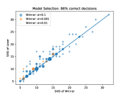
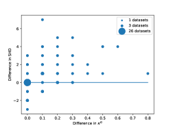
Figure 10: We used the self-compatibility score $\kappa^{I}$ for model selection of the RCD algorithm with different $\alpha$ thresholds.

A.12.3 Additional real data

We first applied our self-compatibility scores to the dataset presented by Sachs et al. [2005].

We compare the SHD of ${\cal A}({\bf X})$ for all algorithms ${\cal A}$ and also the $F_{1}$ score with respect to the existence of an edge in the skeleton of the resulting graph. It is worth noting, that the SHD (and also $\kappa^{G}$) of different model types like ADMGs, PAGs and CPDAGs are not directly comparable.

We started by using the RCD algorithm as we suspected the real dataset might contain confounding and the LiNGAM based method does not merely return a Markov equivalence class. We used the interventional compatibility measure $\kappa^{I}$ since RCD also assumes linearity and also $\kappa^{G}$. As we can see in table 1, the interventional compatibility score is very high, especially compared to the results in figure 2 (i.e. compared to a setting where the assumptions of RCD are fulfilled). This lead us to the conclusion that probably either linearity or the non-Gaussian additive noise assumption are violated. We therefore tried FCI with the correlation-based Fisher $Z$ test and used again the interventional score $\kappa^{I}$ and the graphical score $\kappa^{G}$. Again, this performed very poorly with respect to the interventional self-compatibility score. So as a third attempt, we tried FCI with the kernel-based independence test proposed by [Zhang et al., 2011] and (as we cannot use $\kappa^{I}$ in a non-linear setting) we only report $\kappa^{G}$. This yielded a better self-compatibility score. But as the SHD of 20, which is still comparably high, shows, the good self-compatibility score is not enough to guarantee a good performance. We additionally wanted to try the PC algorithm such that we might be able to falsify the sufficiency assumption. This actually led to the best results in our experiments in terms of $\kappa^{G}$. Overall, this exemplary workflow guided us through model selection decisions and led to an improvement in both, SHD and the skeleton $F_{1}$ score.

Table 1: Comparison of Causal Discovery Algorithms on Cell Dataset

	RCD	FCI + Fisher $Z$	FCI + KCI	PC + KCI
$\kappa^{I}$	0.964	0.81	-	-
$\kappa^{G}$	1.63	5.7	0.2	0
SHD	24	62	26	20
Skeleton $F_{1}$	0.45	0.52	0.57	0.57

We also repeated the real data experiment from section 4 with the climate dataset from Huang et al. [2021]. Again, we compare the SHD of ${\cal A}({\bf X})$ for all algorithms ${\cal A}$ and also the $F_{1}$ score with respect to the existence of an edge in the skeleton of the resulting graph.

In this experiment, all algorithms yielded rather unstable results. But as the SHD and skeleton $F_{1}$ score are also bad for all of them, this result seems reasonable. The ground truth graph provided by Huang et al. [2021] is not a DAG. In order to be able to compare the resulting PAG of FCI with another PAG, we randomly dropped edges from cycles in the ground truth graph, derived the respective PAG and calculated the SHD between these PAGs. For CPDAGs we interpreted the ground truth graph as a CPDAG when we evaluated the SHD.

Table 2: Comparison of Causal Discovery Algorithms on Climate Dataset

	RCD	FCI + Fisher $Z$	FCI + KCI	PC + KCI
$\kappa^{I}$	1.0	0.75	-	-
$\kappa^{G}$	4.0	9.25	6.1	6.625
SHD	51	62	63	43
Skeleton $F_{1}$	0.51	0.5	0.35	0.39

References

- Bollen and Ting [1993] K. A. Bollen and K.-f. Ting. Confirmatory tetrad analysis. Sociological methodology, pages 147–175, 1993.
- Bousquet and Elisseeff [2002] O. Bousquet and A. Elisseeff. Stability and generalization. The Journal of Machine Learning Research, 2:499–526, 2002.
- Bousquet et al. [2020] O. Bousquet, Y. Klochkov, and N. Zhivotovskiy. Sharper bounds for uniformly stable algorithms. In Conference on Learning Theory, pages 610–626. PMLR, 2020.
- Chickering [2002] D. M. Chickering. Optimal structure identification with greedy search. Journal of machine learning research, 3(Nov):507–554, 2002.
- Claassen and Heskes [2012] T. Claassen and T. Heskes. A bayesian approach to constraint based causal inference. arXiv preprint arXiv:1210.4866, 2012.
- Daley et al. [2022] P. J. Daley, K. J. Resch, and R. W. Spekkens. Experimentally adjudicating between different causal accounts of bell-inequality violations via statistical model selection. Physical Review A, 105(4):042220, 2022.
- Daniusis et al. [2010] P. Daniusis, D. Janzing, J. M. Mooij, J. Zscheischler, B. Steudel, K. Zhang, and B. Schölkopf. Inferring deterministic causal relations. In Proceedings of the 26th Annual Conference on Uncertainty in Artificial Intelligence (UAI), pages 143–150. AUAI Press, 2010.
- Darmois [1953] G. Darmois. Analyse générale des liaisons stochastiques. Rev. Inst. Internationale Statist., 21:2–8, 1953.
- Dawid [2021] P. Dawid. Decision-theoretic foundations for statistical causality. Journal of Causal Inference, 9(1):39–77, 2021. doi: doi:10.1515/jci-2020-0008. URL https://doi.org/10.1515/jci-2020-0008.
- Eulig et al. [2023] E. Eulig, A. A. Mastakouri, P. Blöbaum, M. Hardt, and D. Janzing. Toward falsifying causal graphs using a permutation-based test, 2023.
- Evans and Richardson [2014] R. J. Evans and T. S. Richardson. Markovian acyclic directed mixed graphs for discrete data. 2014.
- Gettier [1963] E. Gettier. Is knowledge justified true belief? Analysis, 23(6):121–123, 1963.
- Gresele et al. [2022] L. Gresele, J. Von Kügelgen, J. Kübler, E. Kirschbaum, B. Schölkopf, and D. Janzing. Causal inference through the structural causal marginal problem. In International Conference on Machine Learning, pages 7793–7824. PMLR, 2022.
- Guo et al. [2023] S. Guo, J. Wildberger, and B. Schölkopf. Out-of-variable generalization. arXiv preprint arXiv:2304.07896, 2023.
- Heckerman [1995] D. Heckerman. A Bayesian approach to learning causal networks. In Proceedings of the 11th Conference on Uncertainty in Artificial Intelligence, pages 285–295, San Francisco, CA, 1995. Morgan Kaufmann Publishers.
- Hoyer et al. [2008a] P. Hoyer, D. Janzing, J. M. Mooij, J. Peters, and B. Schölkopf. Nonlinear causal discovery with additive noise models. Advances in neural information processing systems, 21, 2008a.
- Hoyer et al. [2008b] P. O. Hoyer, S. Shimizu, A. J. Kerminen, and M. Palviainen. Estimation of causal effects using linear non-gaussian causal models with hidden variables. International Journal of Approximate Reasoning, 49(2):362–378, 2008b.
- Huang et al. [2021] Y. Huang, M. Kleindessner, A. Munishkin, D. Varshney, P. Guo, and J. Wang. Benchmarking of data-driven causality discovery approaches in the interactions of arctic sea ice and atmosphere. Frontiers in big Data, 4:642182, 2021.
- Imbens [2020] G. W. Imbens. Potential outcome and directed acyclic graph approaches to causality: Relevance for empirical practice in economics. Journal of Economic Literature, 58(4):1129–79, December 2020.
- Janzing [2018] D. Janzing. Merging joint distributions via causal model classes with low vc dimension. arXiv preprint arXiv:1804.03206, 2018.
- Janzing [2019] D. Janzing. The cause-effect problem: Motivation, ideas, and popular misconceptions. In I. Guyon, R. Statnikov, and B. Bakir Batu, editors, Cause Effect Pairs in Machine Learning, pages 3–26. Springer, 2019.
- Kalisch and Bühlman [2007] M. Kalisch and P. Bühlman. Estimating high-dimensional directed acyclic graphs with the pc-algorithm. Journal of Machine Learning Research, 8(3), 2007.
- Lachapelle et al. [2020] S. Lachapelle, P. Brouillard, T. Deleu, and S. Lacoste-Julien. Gradient-based neural dag learning, 2020.
- Lu and White [2014] X. Lu and H. White. Robustness checks and robustness tests in applied economics. Journal of Econometrics, 178:194–206, 2014. URL https://www.sciencedirect.com/science/article/pii/S0304407613001668. Annals Issue: Misspecification Test Methods in Econometrics.
- Maeda and Shimizu [2020a] T. N. Maeda and S. Shimizu. Rcd: Repetitive causal discovery of linear non-gaussian acyclic models with latent confounders. In S. Chiappa and R. Calandra, editors, Proceedings of the Twenty Third International Conference on Artificial Intelligence and Statistics, volume 108 of Proceedings of Machine Learning Research, pages 735–745. PMLR, 26–28 Aug 2020a.
- Maeda and Shimizu [2020b] T. N. Maeda and S. Shimizu. Rcd: Repetitive causal discovery of linear non-gaussian acyclic models with latent confounders. In International Conference on Artificial Intelligence and Statistics, pages 735–745. PMLR, 2020b.
- Marx and Vreeken [2017] A. Marx and J. Vreeken. Telling cause from effect using mdl-based local and global regression. In 2017 IEEE International Conference on Data Mining, ICDM 2017, New Orleans, LA, USA, November 18-21, 2017, pages 307–316, 2017.
- Mukherjee et al. [2006] S. Mukherjee, P. Niyogi, T. Poggio, and R. Rifkin. Learning theory: stability is sufficient for generalization and necessary and sufficient for consistency of empirical risk minimization. Advances in Computational Mathematics, 25:161–193, 2006.
- Ng et al. [2020] I. Ng, A. Ghassami, and K. Zhang. On the role of sparsity and dag constraints for learning linear dags. In H. Larochelle, M. Ranzato, R. Hadsell, M. Balcan, and H. Lin, editors, Advances in Neural Information Processing Systems, volume 33, pages 17943–17954. Curran Associates, Inc., 2020. URL https://proceedings.neurips.cc/paper_files/paper/2020/file/d04d42cdf14579cd294e5079e0745411-Paper.pdf.
- Oster [2019] E. Oster. Unobservable selection and coefficient stability: Theory and evidence. Journal of Business & Economic Statistics, 37(2):187–204, 2019.
- Pearl [2009] J. Pearl. Causality. Cambridge university press, 2009.
- Pearl and Mackenzie [2018] J. Pearl and J. Mackenzie. The book of why. Basic Books, USA, 2018.
- Pearl and Verma [1995] J. Pearl and T. S. Verma. A theory of inferred causation. In Studies in Logic and the Foundations of Mathematics, volume 134, pages 789–811. Elsevier, 1995.
- Perković et al. [2015] E. Perković, J. Textor, M. Kalisch, and M. H. Maathuis. A complete generalized adjustment criterion. In Proceedings of the Thirty-First Conference on Uncertainty in Artificial Intelligence, pages 682–691, 2015.
- Peters et al. [2017] J. Peters, D. Janzing, and B. Schölkopf. Elements of causal inference: foundations and learning algorithms. The MIT Press, 2017.
- Popper [1959] K. Popper. The logic of scientific discovery. Routledge, London, 1959.
- Reisach et al. [2021] A. Reisach, C. Seiler, and S. Weichwald. Beware of the simulated dag! causal discovery benchmarks may be easy to game. In M. Ranzato, A. Beygelzimer, Y. Dauphin, P. Liang, and J. W. Vaughan, editors, Advances in Neural Information Processing Systems, volume 34, pages 27772–27784. Curran Associates, Inc., 2021. URL https://proceedings.neurips.cc/paper_files/paper/2021/file/e987eff4a7c7b7e580d659feb6f60c1a-Paper.pdf.
- Reynolds et al. [2022] R. J. Reynolds, R. T. Scott, R. T. Turner, U. T. Iwaniec, M. L. Bouxsein, L. M. Sanders, and E. L. Antonsen. Validating causal diagrams of human health risks for spaceflight: An example using bone data from rodents. Biomedicines, 10(9):2187, 2022.
- Richardson [2003] T. Richardson. Markov properties for acyclic directed mixed graphs. Scandinavian Journal of Statistics, 30(1):145–157, 2003.
- Richardson et al. [2023] T. S. Richardson, R. J. Evans, J. M. Robins, and I. Shpitser. Nested markov properties for acyclic directed mixed graphs. The Annals of Statistics, 51(1):334–361, 2023.
- Sachs et al. [2005] K. Sachs, O. Perez, D. Pe’er, D. A. Lauffenburger, and G. P. Nolan. Causal protein-signaling networks derived from multiparameter single-cell data. Science, 308(5721):523–529, 2005.
- Shalev-Shwartz et al. [2010] S. Shalev-Shwartz, O. Shamir, N. Srebro, and K. Sridharan. Learnability, stability and uniform convergence. The Journal of Machine Learning Research, 11:2635–2670, 2010.
- Shimizu et al. [2006] S. Shimizu, P. O. Hoyer, A. Hyvärinen, A. Kerminen, and M. Jordan. A linear non-gaussian acyclic model for causal discovery. Journal of Machine Learning Research, 7(10), 2006.
- Shimizu et al. [2011] S. Shimizu, T. Inazumi, Y. Sogawa, A. Hyvarinen, Y. Kawahara, T. Washio, P. O. Hoyer, K. Bollen, and P. Hoyer. Directlingam: A direct method for learning a linear non-gaussian structural equation model. Journal of Machine Learning Research-JMLR, 12(Apr):1225–1248, 2011.
- Skitovic [1962] V. Skitovic. Linear combinations of independent random variables and the normal distribution law. Select. Transl. Math. Stat. Probab., (2):211–228, 1962.
- Spirtes and Scheines [2004] P. Spirtes and R. Scheines. Causal inference of ambiguous manipulations. Philosophy of Science, 71(5):833–845, 2004. doi: 10.1086/425058.
- Spirtes et al. [1999] P. Spirtes, C. Meek, and T. Richardson. An algorithm for causal inference in the presence of latent variables and selection bias. Computation, causation, and discovery, 21:211–252, 1999.
- Spirtes et al. [2000] P. Spirtes, C. N. Glymour, R. Scheines, and D. Heckerman. Causation, prediction, and search. MIT press, 2000.
- Strobl et al. [2016] E. V. Strobl, P. L. Spirtes, and S. Visweswaran. Estimating and controlling the false discovery rate for the pc algorithm using edge-specific p-values. arXiv preprint arXiv:1607.03975, 2016.
- Su and Henckel [2022] Z. Su and L. Henckel. A robustness test for estimating total effects with covariate adjustment. In Uncertainty in Artificial Intelligence, pages 1886–1895. PMLR, 2022.
- Textor et al. [2017] J. Textor, B. van der Zander, M. S. Gilthorpe, M. Liśkiewicz, and G. T. Ellison. Robust causal inference using directed acyclic graphs: the R package ‘dagitty’. International Journal of Epidemiology, 45(6):1887–1894, 01 2017. ISSN 0300-5771. doi: 10.1093/ije/dyw341. URL https://doi.org/10.1093/ije/dyw341.
- Tian and Pearl [2002] J. Tian and J. Pearl. A general identification condition for causal effects. In Aaai/iaai, pages 567–573, 2002.
- Triantafillou and Tsamardinos [2016] S. Triantafillou and I. Tsamardinos. Score-based vs constraint-based causal learning in the presence of confounders. In Cfa@ uai, pages 59–67, 2016.
- Tsamardinos et al. [2012] I. Tsamardinos, S. Triantafillou, and V. Lagani. Towards integrative causal analysis of heterogeneous data sets and studies. The Journal of Machine Learning Research, 13(1):1097–1157, 2012.
- Verma and Pearl [2022] T. S. Verma and J. Pearl. Equivalence and synthesis of causal models. In Probabilistic and Causal Inference: The Works of Judea Pearl, pages 221–236. 2022.
- Vorob’ev [1962] N. Vorob’ev. Consistent families of measures and their extensions. Theory Probab. Appl, 7(2):147–163, 1962.
- Walter and Tiemeier [2009] S. Walter and H. Tiemeier. Variable selection: current practice in epidemiological studies. European journal of epidemiology, 24:733–736, 2009.
- Zhang [2008] J. Zhang. Causal reasoning with ancestral graphs. Journal of Machine Learning Research, 9:1437–1474, 2008.
- Zhang and Hyvärinen [2009] K. Zhang and A. Hyvärinen. On the identifiability of the post-nonlinear causal model. In Proceedings of the 25th Conference on Uncertainty in Artificial Intelligence, Montreal, Canada, 2009.
- Zhang et al. [2011] K. Zhang, J. Peters, D. Janzing, and B. Schölkopf. Kernel-based conditional independence test and application in causal discovery. In 27th Conference on Uncertainty in Artificial Intelligence (UAI 2011), pages 804–813. AUAI Press, 2011.
- Zheng et al. [2020] X. Zheng, C. Dan, B. Aragam, P. Ravikumar, and E. Xing. Learning sparse nonparametric dags. In S. Chiappa and R. Calandra, editors, Proceedings of the Twenty Third International Conference on Artificial Intelligence and Statistics, volume 108 of Proceedings of Machine Learning Research, pages 3414–3425. PMLR, 26–28 Aug 2020.