Spatio-temporal quasi-experimental methods for rare disease outcomes: The impact of reformulated gasoline on childhood hematologic cancer

Abstract

Although some pollutants emitted in vehicle exhaust, such as benzene, are known to cause leukemia in adults with high exposure levels, less is known about the relationship between traffic-related air pollution (TRAP) and childhood hematologic cancer. In the 1990s, the US EPA enacted the reformulated gasoline program in select areas of the US, which drastically reduced ambient TRAP in affected areas. This created an ideal quasi-experiment to study the effects of TRAP on childhood hematologic cancers. However, existing methods for quasi-experimental analyses can perform poorly when outcomes are rare and unstable, as with childhood cancer incidence. We develop Bayesian spatio-temporal matrix completion methods to conduct causal inference in quasi-experimental settings with rare outcomes. Selective information sharing across space and time enables stable estimation, and the Bayesian approach facilitates uncertainty quantification. We evaluate the methods through simulations and apply them to estimate the causal effects of TRAP on childhood leukemia and lymphoma.

Keywords: causal inference; childhood leukemia; childhood lymphoma; matrix completion; panel data; traffic-related air pollution

1 Introduction

Traffic-related air pollution (TRAP) has long been a suspected risk factor for childhood hematologic cancers. Pollutants emitted in vehicle exhaust, such as benzene and 1,3-butadiene, are known to cause leukemia in adults with high occupational exposure levels [1, 2], but meta-analyses and reviews of the large literature studying the relationship between ambient TRAP and pediatric hematologic cancer have failed to establish a causal relationship [3, 4, 5, 6]. The inconclusive results are likely due to the rarity of childhood cancer, the difficulty in measuring ambient TRAP exposure and exposure timing, and confounding [7, 8].

In the 1990s, in an effort to control TRAP, the US EPA enacted gasoline content regulations in select heavily-polluted areas of the US. In particular, the regulations mandated that only reformulated gasoline be sold in these areas. In reformulated gasoline, the allowable benzene content was capped at 1% by volume, and it was required to contain at least 2% oxygen via the use of an oxygenate (such as ethanol) [9]. The reformulated gasoline was intended to reduce volatile organic compound and toxic air pollutant emissions by 15% when compared to conventional gasoline, without increasing NO_x emissions [9]. This new limit on mobile-source benzene induced substantial declines in ambient TRAP in affected areas. For example, California began selling reformulated gasoline between 1995-1996. It is estimated that ambient benzene concentrations decreased by 30%-40% between 1994-1996 as a result [10, 11]. These reformulated gasoline regulations created an ideal quasi-experiment (QE) to study the effects of TRAP on childhood hematologic cancer incidence, as regulated areas experienced sudden changes in exposure while many nearby areas did not. Quasi-experimental studies are advantageous in environmental health contexts because they enable use of inexpensive panel data and leverage localized exposure changes to estimate health effects adjusted for certain types of unmeasured confounding. In this paper, our aim is to develop analytic and inferential methods for quasi-experimental studies with rare disease incidence outcomes and apply these methods to study the impact of the reformulated gasoline program on childhood hematologic cancer incidence.

A wide range of approaches, relying on different causal identifying assumptions, have been proposed for estimating effects in QE settings. Difference-in-differences is a widely-used approach that relies on the parallel trends assumption, which states the difference in outcomes in the treated and control groups would have remained constant over the study period in the absence of treatment. Parallel trends can also be described as the assumption of no time-varying unmeasured confounders. Under this assumption, causal effects are estimated by comparing the observed outcome trend in the control group to the observed outcome trend in the treatment group. However, in the presence of time-varying confounders, the parallel trends assumption is violated. This limitation gave rise to the synthetic control method [12], which controls for certain types of time-varying confounders by leveraging pre-treatment temporal trends in treated and control units. It achieves this by reweighting control units to construct a "synthetic control unit" whose post-treatment outcomes serve as the counterfactual outcomes for a single treated unit. The weights are constructed to ensure that pre-treatment trends in the synthetic control unit mimic those in the treated unit, which accounts for trends induced by certain time-varying confounders.

In recent years, various methods have been introduced to improve or extend difference-in-differences and synthetic control methods. Doubly-robust approaches to effect estimation in QE settings have been proposed [13, 14], which utilize two different modeling strategies to adjust for confounding bias, and are able to recover causal effects if either model is correctly specified. The Augmented Synthetic Control Method [15] adds a bias-correction to the standard synthetic control method to improve causal effect estimates when the synthetic control unit does not adequately capture pre-treatment trends in the treated unit.

An adjacent literature has emerged proposing causal inference methods for QEs with panel data that model outcomes explicitly, then employ these models to impute missing counterfactual outcomes. In this paper, we build on the matrix completion (MC) approach for causal inference with panel data, proposed by Athey et al [16] (a closely related approach called generalized synthetic controls was introduced by Xu et al. [17]). Like synthetic controls, this method leverages temporal trends in treated and control units to adjust for time-varying unmeasured confounders, but it allows for multiple treatment units and variable treatment initiation times. The approach proceeds as follows: (1) structure the panel data into a matrix; (2) set outcomes for treated units during post-treatment period to missing to create a matrix of outcomes under control; (3) apply MC to this matrix to obtain a low-rank matrix factorization; (4) use the matrix factorization to impute the missing outcomes in the matrix. The imputed outcomes represent estimates of the counterfactuals, i.e., the outcomes expected in the treated units at post-treatment times, in the absence of treatment. MC can adjust for time-varying unmeasured confounders, so long as their temporal trends do not change differentially in treated and control units at post-treatment times.

MC and synthetic control methods rely heavily on capturing pre-treatment trends in outcomes in order to adjust for confounding. The performance of these methods has not been evaluated in the context of rare disease outcome data, where trends are unstable and noisy. However, because they rely on either stable patterns across time or stable patterns across units [16], they are unlikely to be able to properly adjust for confounding when outcomes are rare and trends are highly impacted by noise.

Another limitation of standard MC and synthetic control methods is the lack of reliable, finite sample inferential tools. In synthetic control methods, researchers can, in some cases, perform inference using a permutation test [18]. However, these tests often fail, as the requisite symmetry assumption for permutation tests is commonly violated [18]. Recently, Chernozhukov et al. [19] make use of ideas from conformal prediction and permutation tests for an inference procedure that can be generalized for many different panel data methods. A very limited recent literature has begun to explore Bayesian implementations of MC for panel data [20, 21]. The Bayesian approach is advantageous relative to frequentist implementations, as inference does not require strict assumptions and can be provided in a consistent and straightforward procedure through the posterior predictive distribution of treated units’ counterfactuals [21, 20, 22].

Integrating concepts from the Bayesian disease mapping and latent factor model literatures, we seek to extend MC methods to enable robust investigation of the impacts of environmental QEs on rare disease outcomes. Our main contributions are (1) evaluating the performance of existing MC and synthetic control methods in rare outcome contexts and (2) proposing alternative Bayesian MC approaches using spatio-temporal smoothing, regularization, and adaptive hyperparameter selection to reduce over-fitting and improve estimation in this setting. Through an extensive simulation study designed to mimic real disease outcome scenarios, we assess the performance of our proposed methods and compare them to existing MC and synthetic control methods. We then apply these methods to study the effects of TRAP on the incidence of childhood and young adult leukemia and lymphoma using the reformulated gasoline program QE described above. Although our methods are directly motivated by this case study, they can be used more generally when trends in outcomes are unstable/noisy or when spatial or temporal correlation is expected.

2 Methods

2.1 Motivating Data

The federal reformulated gasoline program targeted areas with severe ozone problems, mandating the sale of exclusively reformulated gasoline in certain metropolitan counties within the following states: California, Connecticut, New Jersey, New York, Delaware, Maryland, Pennsylvania, Indiana, Texas, and Wisconsin. The full list of counties included in the program is shown in Supplemental Table S6 [23]. The program took effect in 1995 for the counties listed in this table. The state of California also implemented its own reformulated gasoline program, requiring that gasoline with similar requirements to the federal reformulated gasoline be sold statewide [24], which went into effect in the summer of 1996.

In general, in our analyses, we consider a county to be “treated” if and when the reformulated gasoline program went into effect there. However, because some counties in California began using reformulated gasoline in 1995 and others in 1996, there is concern of spillover effects during the interim period. It is possible the effect of using the reformulated gas spilled over to counties that hadn’t enacted the regulation (or vice-versa) through commuting and migration. Additionally, there is concern of anticipation. It is possible some gas stations in untreated California counties in 1995 began selling reformulated gasoline in anticipation of the program implementations. For this reason, in our primary analyses we consider the entire state of California to have been treated starting in 1995.

The study period of interest is 1988 to 2003, to incorporate a substantial number of years pre- and post-treatment to discern trends in the outcome. We rely primarily on childhood and young adult (CYA) leukemia and lymphoma incidence data from the National Cancer Institute’s Surveillance Epidemiology End Result (SEER) database [25]. During the study period, 9 unique cancer registries contributed population-level data to SEER, covering the following areas: San Francisco Bay Area (California), Connecticut, Atlanta (Georgia), Hawaii, Iowa, Detroit (Michigan), New Mexico, Utah, and Seattle-Puget Sound (Washington). Note that the SEER-covered areas include counties that were both treated and untreated in the reformulated gasoline program.

Due to differing data availability by disease type, the analyses for leukemia and lymphoma cover slightly different study areas. For lymphoma, only SEER data are available, so the study area is the SEER-covered areas listed above. The treated counties in the lymphoma analyses thus consist of 5 California counties and 8 Connecticut counties. The control counties are the remaining 155 counties SEER-covered counties in Georgia, Hawaii, Idaho, Minnesota, New Mexico, Utah, and Washington. For leukemia, in addition to SEER, we have access to incidence data from the California Cancer Registry during the study period, which covers all California counties. Thus, we make use of both data sources in the leukemia analyses, and the set of treated counties is expanded in the leukemia analyses to include all 52 California counties.

From these data sources, annual county-level leukemia and lymphoma incidence rates were constructed. Childhood leukemia is most commonly diagnosed in children ages 1-4, and over 60% of new cases occur in children $<10$ years old [25]. Moreover, leukemia cases occurring in younger and older children tend to be biologically distinct [26, 27]. For these reasons, we study leukemia incidence among children ages 0-9, exclusively. The epidemiology of lymphoma in children and young adults is quite different from leukemia, with risk increasing monotonically up to the mid-to-late 20s [28]. Thus, for our lymphoma analyses, we investigate incidence among 0-29 year olds.

Although MC can, in principle, adjust for time-varying unmeasured confounders that do not change differentially in treated and control units post-treatment, we explicitly control for one time-varying potential confounder in our analyses that may violate this condition: county-level percent Hispanic children and young adults. Hispanic children in the US are known to be at higher risk for hematologic malignancies [29], and the size of the Hispanic population is likely to have been changing differentially in treated and control areas during our study period. Thus, to avoid possible residual confounding from this variable after applying MC, we explicitly adjust for it in our analyses using data retrieved from the U.S. Census Bureau.

2.2 Notation and Matrix Completion

Consider our CYA cancer incidence panel data. Let $i=1,...,N$ index the counties of interest where $N$ is the number of counties and $t=1,...,T$ index the time periods in years where $T$ is the last year of the study. Suppose the outcome data are arranged into an $N\times T$ panel matrix, with counties in the rows and years in the columns. The observed outcome for county $i$ at time $t$ can be denoted as $Y_{it}$. Let $\mathcal{W}$ denote the set of indices for treated units and let $n_{\mathcal{W}}$ denote the size of the treated group.

We situate our approaches within the potential outcomes framework [30], such that $Y_{it}(1)$ and $Y_{it}(0)$ denote the outcomes that would have been observed in county $i$ at time $t$ under treatment and control, respectively. For $(i,t)\in\mathcal{W}$, $Y_{it}$=$Y_{it}(1)$ , i.e., the observed outcome is equal to the potential outcome under treatment for treated units at post-treatment times (Figure 1). Conversely, for $(i,t)\notin\mathcal{W}$, $Y_{it}$=$Y_{it}(0)$. Because $Y_{it}(0)$ is unobserved for the treated units at post-treatment times, the aim of the methods introduced in this paper is to estimate $Y_{it}(0)$ for these units (which are then used to estimate treatment effects, i.e., $Y_{it}(1)-\widehat{Y}_{it}(0)=Y_{it}-\widehat{Y}_{it}(0)$). For the models used throughout this paper, we follow the causal identifying assumptions for Bayesian matrix completion as described by Tanaka et al., Nethery et al., and Pang et al. [21, 22, 20]. That is, we assume the stable unit treatment value assumption (SUTVA) [31], causal consistency, latent ignorability, the unobserved time-varying confounders can be captured by a small number of latent factors, and conditional exchangeability.

In the formulation of MC methods for causal inference with QEs, the matrix with missing values is the matrix of $Y_{it}(0)$, denoted $\mathbf{Y(0)}$. This is simply the panel data matrix with entries in the positions corresponding to the treated units at post-treatment times artificially set to missing. In Athey et al. [16], the missing post-treatment $Y_{it}(0)$ values are imputed using the factors obtained from a low-rank factorization of the matrix $\mathbf{Y(0)}$ into a matrix of time-specific latent factors $\mathbf{V}$ and unit-specific factor loadings $\mathbf{U}$. The MC model takes the form $Y_{it}(0)=\mathbf{U}_{i}^{T}\mathbf{V}_{t}+\epsilon_{it}$. Here, $\mathbf{U}_{i}$ is a $K$-length vector of county-specific latent factors, $\mathbf{V}_{t}$ is a $K$-length vector of unknown time-specific factor loadings, and $K$ is an unknown scalar with $K\leq\leq\mathrm{min}(N,T)$. The matrices $\mathbf{U}\in\mathbb{R}^{K\times N}$ and $\mathbf{V}\in\mathbb{R}^{K\times T}$ aim to capture unmeasured confounders in the data.

To implement MC in a Bayesian framework, one can use a likelihood of the form:

$$P(\mathbf{Y(0)}\mid\mathbf{U},\mathbf{V},\Sigma)=\prod_{i}\prod_{t}[f(Y_{it}(0)|\mathbf{U}_{i}^{T}\mathbf{V}_{t},\Sigma)]\times\mathrm{I}[(i,t)\in\mathcal{O}]$$ (1)

where $f$ is the pmf or pdf of the response with mean given by $\mathbf{U}_{i}^{T}\mathbf{V}_{t}$ and common scale parameter $\Sigma$. Often, Gaussian priors with means $\mu_{U}$ and $\mu_{V}$ and precision matrices $\Lambda^{-1}_{U}$ and $\Lambda^{-1}_{V}$ are placed on $\mathbf{U}$ and $\mathbf{V}$, respectively [32].

The posterior predictive distribution for the missing values, $\mathbf{Y(0)}^{mis}$, is obtained by conditioning on the observed values, $\mathbf{Y(0)}^{obs}$, and marginalizing over the model parameters and hyperparameters:

$$P(\mathbf{Y(0)}^{mis}\mid\mathbf{Y(0)}^{obs})=\int P(\mathbf{Y(0)}^{mis}\mid\mathbf{U},\mathbf{V},\Sigma)\ P(\mathbf{U},\mathbf{V},\Sigma\mid\mathbf{Y(0)}^{obs})\ d(\mathbf{U},\mathbf{V},\Sigma)$$

Exact evaluation of this predictive distribution is analytically intractable. Instead, MCMC based methods can use a Monte Carlo approximation to the predictive distribution by:

$$P(\mathbf{Y(0)}^{mis}\mid\mathbf{Y(0)}^{obs})\approx\frac{1}{M}\sum^{M}_{m=1}P(\mathbf{Y(0)}^{mis}\mid\mathbf{U}^{(m)},\mathbf{V}^{(m)},\Sigma)$$

where the samples of $\{\mathbf{U}^{(m)},\mathbf{V}^{(m)}\}$ are generated by running a Markov Chain whose stationary distribution is the posterior distribution over the model parameters and hyperparameters [32]. Here, $\mathbf{U}$ and $\mathbf{V}$ are not identifiable without further constraints [21]. However, in the Bayesian context, this does not compromise the identifiability of the predictions from the model [22].

2.3 Matrix Completion Approaches for Rare Count Outcomes

Our model builds on the Bayesian MC models for Poisson/count data [33, 34, 35, 22] by tailoring it to QE analysis settings with rare outcomes, which are common in small-area cancer incidence data, and to accommodate complex spatio-temporal correlation structures in the outcomes. First, by taking a Bayesian approach, our models inherently regularize, which may help prevent over-fitting noisy data. Second, to account for the instability in trends over space and time that often occur with rare outcome data and may compromise MC’s ability to adjust for unmeasured confounders, we introduce spatio-temporal priors into relevant components of the MC model (Figure 1). The addition of these priors will help stabilize trends by sharing information across space and time. In the context of environmental exposures and disease outcomes, any unmeasured confounders (represented by the $\mathbf{U}$ and $\mathbf{V}$ matrices) would likely have a spatio-temporal structure. By explicitly encoding this structure into the $\mathbf{U}$ and $\mathbf{V}$ matrices, the model is more likely to uncover these confounders. In some of our models, we also include a shrinkage prior that allows for adaptive selection of $K$, which reduces the chances of model misspecification.

Figure 1: Illustration of spatio-temporal matrix completion. $c_{it}$ denotes all other components of the mean model.

The various model formulations we will propose leverage differing prior distributions but all impose the following mean structure for the $Y_{it}(0)$, which is similar to that of [22]:

$$\mathrm{log}\left(E\left[Y_{it}(0)\right]\right)=\alpha+\gamma_{i}+\psi_{t}+\mathbf{U}_{i}^{T}\mathbf{V}_{t}+\mathbf{X}_{it}^{\prime}\boldsymbol{\beta}+\mathrm{log}(\theta_{\mathrm{it}})$$ (2)

where $\alpha$ is a global intercept, $\gamma_{i}$ are county-specific deviations from the global intercept, $\psi_{t}$ are time-specific deviations from the global intercept, $\mathbf{U}_{i}$ and $\mathbf{V}_{t}$ are defined as above, $\mathbf{X}_{it}$ is a vector of time-varying measured confounders (if any) and $\boldsymbol{\beta}$ is a vector of their coefficient parameters, and $\theta_{it}$ is a scalar offset of the population size at county $i$ and time point $t$. This model extends classic Bayesian MC methods by allowing for a non-identity link and an offset, all of which are critical when modeling and predicting the incidence of rare diseases.

Since we are using count data in our application, our likelihood will take the form of equation (1) where $f$ is the negative binomial pmf with mean given by equation (2) and common scale parameter $\Sigma$. The missing entries in $\mathbf{Y(0)}$ are then sampled from the posterior predictive distribution using the rstan R package [36]. We then construct MCMC samples of the ATT for each treated time as:

$$\mathrm{ATT}_{t}^{(m)}=\frac{1}{N_{\mathcal{W}}}\sum_{i\in W}\Big{[}Y_{it}(1)-Y_{it}^{(m)}(0)\Big{]}$$

where $Y_{it}^{(m)}(0)$ is the $m^{\mathrm{th}}$ MCMC sample of $Y_{it}(0)$. Using summaries of the MCMC samples, we can estimate $\mathrm{ATT}_{t}$ and its uncertainties.

With panel data, the success of MC models depends on the ability of the model to capture trends over space and time. Taking this into account, prior distributions on the latent factors and factor loadings matrices that account for spatio-temporal correlation will be utilized. That is, we consider spatial priors for the county-specific factor loadings in the rows of $\mathbf{U}$ ($\mathbf{U}_{k}$, $k=1,...,K$) and temporal priors on the time-specific latent factors in the rows of $\mathbf{V}$ ($\mathbf{V}_{k}$). Additionally, non-informative priors are specified for $\Sigma$, $\alpha$, $\gamma_{i}$, $\psi_{t}$, and $\beta$ i.e. $\Sigma\sim\mathrm{Unif}(0,\infty)$ and $\alpha,\gamma_{i},\psi_{t},\beta\sim\mathrm{Unif}(-\infty,\infty)$.

In spatio-temporal models for areal data, spatially structured parameters and/or latent variables are typically obtained using variations of conditional autoregressive priors. Here, to allow for spatial correlation in parameters, we consider the widely-used intrinsic conditional auto-regressive (ICAR) prior, which assumes that the parameter corresponding to a given spatial unit is correlated with the parameters of its neighboring spatial units [37]. Temporally structured parameters are often obtained by specifying auto-regressive priors. In this paper, we consider the first-order auto-regressive prior (AR(1))[38] that accounts for temporal correlation in parameters by using the parameter value from the previous time point to smooth the current time point. We also consider a temporal ICAR prior that assumes the parameter for a given time point is correlated with parameters for both of its neighboring times. See Anderson et al. [39] for an in-depth review of spatio-temporal modeling.

To see how the choice of priors on the latent factors and factor loadings matrices impacts the ability of the model to recover the missing counterfactuals in rare outcome settings, we form six candidate models, characterized by different prior specifications on $\mathbf{U}_{k}$ and $\mathbf{V}_{k}$. We describe each of these models in detail below, and they are also summarized in Table 1.

Table 1: The six Bayesian MC models considered, as defined by different prior specifications on the factors and factor loadings.

Model Name	Model #	Priors on $\mathbf{U_{k}}$	Priors on $\mathbf{V_{k}}$
Vanilla	1	Normal(0,1)	Normal(0,1)
Spatial	2	Spatial ICAR	Normal(0,1)
Space-Time ICAR	3	Spatial ICAR	Temporal ICAR
Space-Time AR(1)	4	Spatial ICAR	Temporal AR(1)
Space-Time Lasso	5	Laplace	Laplace
Space-Time Shrinkage	6	Spatial ICAR	Temporal AR(1)-Shrinkage

2.3.1 Model 1: The Vanilla Model

The Vanilla Model does not formally account for spatial or temporal correlation, placing the conventional independent normal priors on the elements of $\textbf{U}_{k}$ and $\textbf{V}_{k}$, i.e., $\mathbf{U}_{k}\sim\mathrm{N}(\mathbf{0},\mathbf{I}_{N})$ and $\mathbf{V}_{k}\sim\mathrm{N}(\mathbf{0},\mathbf{I}_{T})$, where $\mathbf{I}_{N}$ and $\mathbf{I}_{T}$ are $N\times N$ and $T\times T$ identity matrices, respectively.

2.3.2 Model 2: The Spatial Model

The Spatial Model accounts for spatial correlation through a spatial prior placed on $\textbf{U}_{k}$, but does not account for temporal correlation. In this model, an Intrinsic Conditional Auto-Regressive (ICAR)[37] prior that assumes complete spatial correlation between units is placed on $\textbf{U}_{k}$:

$$\mathbf{U}_{k}\sim\mathrm{N}(0,[\tau(D_{S}-W_{S})]^{-1})$$

where $W_{S}$ is the $N\times N$ spatial adjacency matrix where entries $\{i,i\}$ are zero and the off-diagonal elements are 1 if regions $i$ and $j$ are neighbors and 0 otherwise, and $D_{S}$ is the $N\times N$ diagonal matrix where entries $\{i,i\}$ are the number of neighbors of area $i$ and the off-diagonal entries are 0. We place a $\mathrm{Ga(0.5,0.0005)}$ prior on $\tau$ as suggested by Kelsall and Wakefield [40]. As in the Vanilla Model, standard normal priors are placed on the $\textbf{V}_{k}$.

2.3.3 Model 3: Space-Time ICAR Model

The Space-Time ICAR Model places ICAR priors on the rows of U and V to account for spatial and temporal correlation:

$$\begin{gathered}\mathbf{U}_{k}\sim\mathrm{N}(0,[\tau_{S}(D_{S}-W_{S})]^{-1})\\ \mathbf{V}_{k}\sim\mathrm{N}(0,[\tau_{T}(D_{T}-W_{T})]^{-1})\end{gathered}$$

Here the spatial ICAR prior is as defined in Model 2. In the temporal ICAR prior, $W_{T}$ is the $T\times T$ adjacency matrix where entries $\{i,i\}$ are zero and the off-diagonal elements are 1 if time-point $i$ and $j$ are neighbors and 0 otherwise, and $D_{T}$ is the $T\times T$ diagonal matrix where entries $\{i,i\}$ are the number of neighbors of time-point $i$ and the off-diagonal entries are 0. Additionally, we place $\mathrm{Ga(0.5,0.0005)}$ priors on $\tau_{S}$ and $\tau_{T}$.

2.3.4 Model 4: Space-Time AR Model

The Space-Time AR Model accounts for spatial correlation through the placement of an ICAR prior on the rows of U. To account for temporal correlation in $\mathbf{V}_{k}$, instead of a temporal ICAR prior we specify a First-Order Auto-Regressive prior (AR(1))[38] that takes each point $V_{kt}$ in the rows of $\mathbf{V}$ to be generated according to

$$\begin{gathered}\mathbf{U}_{k}\sim\mathrm{N}(0,[\tau(D_{S}-W_{S})]^{-1})\\ V_{kt}\sim\mathrm{N}(a+b*V_{k(t-1)},\sigma)\\ \end{gathered}$$

Here, improper flat priors (i.e. $\mathrm{Uniform}(-\infty,\infty)$) are placed on the coefficients, $a$ and $b$, and $\sigma$ is a positively constrained noise scale parameter with a $\mathrm{Uniform}(0,\infty)$ prior.

2.3.5 Model 5: Space-Time Lasso Model

The Space-Time Lasso Model induces sparsity by placing independent Laplace distributions as the prior distributions for the rows U and V [41]. These priors have previously been applied to detect clusters in spatial data by selecting groups of points that have similar values for covariates and are adjacent [41]. In our model, the priors encourage the fusion of the loadings and factors for units that are close in space and time, respectively. If we let $C_{S}$ denote a set of all adjacent pairs of spatial units and $C_{T}$ denote a set of all adjacent pairs of temporal units:

$$\begin{gathered}\mathbf{U}_{k}|\lambda_{U1},\lambda_{U2}\sim\prod_{(j,j^{\prime})\in C_{S}}\mathrm{exp}[-\lambda_{U1}|U_{j}-U_{j^{\prime}}|]*\prod^{N}_{i=1}\mathrm{exp}[-\lambda_{U2}|U_{i}|]\\ \mathbf{V}_{k}|\lambda_{V1},\lambda_{V2}\sim\prod_{(j,j^{\prime})\in C_{T}}\mathrm{exp}[-\lambda_{V1}|V_{j}-V_{j^{\prime}}|]*\prod^{T}_{t=1}\mathrm{exp}[-\lambda_{V2}|V_{t}|]\\ \end{gathered}$$

Following Casella et al. [42], we place $\mathrm{Ga}(1,0.1)$ priors on $\lambda_{U1},\lambda_{U2},\lambda_{V1},$ and $\lambda_{V2}$ and enter them into the Gibbs sampler, as this method is fast and leads to posterior means close to the marginal maximum likelihood estimates.

2.3.6 Model 6: Space-Time Shrinkage Model

The Space-Time Shrinkage Model accounts for spatial correlation through the placement of an ICAR prior on the rows of U, as in Models 2 and 3 above. In standard factor models, the need for user-specification of the number of factors, $K$, poses challenges and introduces subjectivity. By specifying a $K$ too large, we risk over-fitting the data and add computational burden, and by specifying a $K$ too small, we have the chance to under-fit and waste information by leaving out important factors. To address this issue and eliminate the need for a user-specified $K$, Bhattacharya and Dunson [43] propose the multiplicative gamma shrinkage prior for latent factor models, which in theory allows for the introduction of infinitely many factors, with the factors increasingly shrunk towards 0 as the row index increases. This is achieved by introducing a scaling factor into the prior variance of the factors that converges towards zero with increasing $K$ at a rate informed by the data. This adaptive selection of $K$ reduces the chances of model misspecification and over-fitting. Here we unify the multiplicative gamma shrinkage prior with the AR(1) prior, to simultaneously account for temporal correlation in $\mathbf{V}_{k}$. To do so, we replace $\sigma$ in the AR(1) prior variance with the multiplicative gamma shrinkage prior. In practice, this model is fit by specifying a value of $K$ believed to be much larger than the true $K$, and the model automatically shrinks the unnecessary factors. The priors for this model can be mathematically formalized as follows:

$$\begin{gathered}\mathbf{U}_{k}\sim\mathrm{N}(0,\tau[D_{S}-W_{S}]^{-1})\\ V_{kt}\mid a,b,\phi_{kt},\eta_{k},V_{k(t-1)}\sim\mathrm{N}\left(a+b*V_{k(t-1)},\phi_{kt}^{-1}\eta_{k}^{-1}\right)\end{gathered}$$

Here, improper flat priors (i.e. $\mathrm{Uniform}(-\infty,\infty)$) are placed on the coefficients, $a$ and $b$. $\phi_{kt}$ is a local shrinkage parameter for the elements in the $K$th row with a $\operatorname{Ga}(\nu/2,\nu/2)$ prior. $\eta_{k}=\prod_{l=1}^{k}\delta_{l}$ is a global shrinkage parameter for the $K$th row. The $\delta_{l}$ $(l=1,\ldots,\infty)$, are independent and $\delta_{1}\sim\mathrm{Ga}\left(a_{1},1\right)$ and $\delta_{l}\sim\mathrm{Ga}\left(a_{2},1\right)$. The $\eta_{k}$s are stochastically increasing under the restriction $a_{2}>1$ as $K$ increases, which favors more shrinkage as the row index increases.

2.4 Data pre-processing for rare outcomes

Due to the potentially extreme temporal instability in rare disease time series, we also consider applying temporal smoothing to the time series from each area as a pre-processing step, prior to their inclusion in the models. Pre-processing of noisy time series prior to formal analysis has long been applied in fields like neuroimaging [44] to improve downstream model performance and ability to detect relevant signals. Here, we consider each of the models described above both with and without a temporal smoothing procedure implemented on data as a pre-processing step. When this pre-processing is applied, we fit a Poisson generalized additive model with a smoothed term on time to each of the time series individually, obtain "smoothed" predictions of the outcome at each time point from the models, and plug those into the MC approach in place of the raw data.

3 Simulations

We conduct extensive simulation studies to evaluate our models’ performance, both relative to one another and relative to the current gold standard approaches, in the context of outcomes mimicking rare and non-rare disease incidence. We compare our methods, implemented in the rstan R package [36], to the standard Athey et al. MC implementation in the gsynth R package [16, 45], the generalized synthetic controls method (GSC) from the gsynth package [17, 45], and the augmented synthetic control method (ASC) from the augsynth package [15, 46] and assess the performance of each method in counterfactual estimation.

3.1 Simulation Structure

Panel data are simulated with $N=29$ counties and $T=15$ years, with $n_{\mathcal{W}}=6$ treated units initiating treatment at year $t=9$, and using a real spatial adjacency matrix for New Mexico’s counties. We generate $K=3$ time varying latent factor vectors $\mathbf{V}_{k}$ and unit-specific factor loading vectors $\mathbf{U}_{k}$ with conditionally autoregressive forms as follows: $\mathbf{U}_{k}\sim\mathrm{N}(\mathbf{0}_{n},\tau^{2}\mathbf{Q}^{-1}\left(\mathbf{W},\rho_{S}\right))$ and $\mathbf{V}_{k}\sim\mathrm{N}(\mathbf{0}_{m},\tau^{2}\mathbf{Q}^{-1}\left(\mathbf{T},\rho_{T}\right))$, with $\tau=.01$. Spatial and temporal correlation are induced in $\mathbf{U}_{k}$ and $\mathbf{V}_{k}$, respectively, through the precision matrices which are defined as in Leroux et al. (2000) [47]:

$$\mathbf{Q}\left(\mathbf{W},\rho_{S}\right)=\rho_{S}[\operatorname{diag}(\mathbf{W1}_{W})-\mathbf{W}]+\left(1-\rho_{S}\right)\mathbf{I}_{N}$$

$$\mathbf{Q}\left(\mathbf{T},\rho_{T}\right)=\rho_{T}[\operatorname{diag}(\mathbf{T1}_{T})-\mathbf{T}]+\left(1-\rho_{T}\right)\mathbf{I}_{T}$$

where $\mathbf{1}_{W}$ and $\mathbf{1}_{T}$ are $N\times 1$ and $T\times 1$ vectors of ones, respectively. Here, $\mathbf{W}$ and $\mathbf{T}$ are spatial and temporal adjacency matrices, respectively, and $\rho_{S}$ and $\rho_{T}$ are common spatial and temporal dependence parameters. In these simulations, we let $\rho_{S}=\rho_{T}=.99$.

The elements of the panel matrix, $\mathbf{Y(0)}$, are simulated from a Poisson distribution with mean $E\left[Y_{it}(0)\right]=\mathrm{exp}(\alpha+\gamma_{i}+\psi_{t}+\mathbf{U}_{i}^{T}\mathbf{V}_{t}+\mathrm{log}(\theta_{\mathrm{it}}))$. The $\theta_{\mathrm{it}}$ are the real population counts for children ages 0 to 9 in the New Mexico county $i$ for time point $t$, extracted from US Census Bureau data, and $\gamma_{i},\psi_{t}\sim N(0,.000015)$. We modified $\alpha$ to obtain simulated data emulating non-rare ($\alpha=-5$) and rare ($\alpha=-7$) outcomes. In each of the rare and non-rare outcome settings, we generated 100 synthetic datasets from the above data generating mechanisms.

We applied Models 1-5 above to each synthetic dataset with 3 different specifications of $K$: one under-specified ($K=1$), one correct ($K=3$), one over-specified ($K=7$). For Model 6 above, we apply it as recommended by Bhattacharya and Dunson [43], specifying only a large value of $K$, $K=7$, in anticipation that it will adaptively shrink away unnecessary factors. 2,000 Hamiltonian Monte Carlo iterations with 1,000 burn-in iterations were collected for each model from rstan [36]. For the competing existing methods, we used the rates themselves as the outcome, since these methods cannot straightforwardly accommodate an offset. For the Athey MC approach we also considered the same three specifications of K. Note that none of the models applied to the data is the “true” data generating model, so here we are evaluating the performance of all the models under some degree of model misspecification. For all of the approaches, we apply and evaluate them with and without the temporal smoothing pre-processing step described in Section 2.4. We fit the smoothing models for each time series using a spline on time with 5 degrees of freedom. To measure performance, we compute the average absolute percent bias in the estimates of the estimated counterfactuals for each approach.

3.2 Results

Table 2: Simulation results: Average absolute percent bias of the counterfactual estimates from each method applied with different specifications of the number of factors, $K$ (rows), in simulated data emulating rare and non-rare outcomes, with and without a temporal smoothing pre-processing step (columns).

Model	K	Non-Rare & Non-Smoothed	Non-Rare & Smoothed	Rare & Non-Smoothed	Rare & Smoothed
Bayesian MC Models
1. Vanilla	1	6.08	5.89	15.76	15.96
	3	6.12	6.04	15.70	16.06
	7	6.50	6.00	17.95	16.86
2. Space	1	5.95	6.59	16.79	16.77
	3	6.88	6.39	20.28	19.89
	7	7.77	7.82	25.38	24.67
3. Space-Time ICAR	1	6.45	6.16	16.79	17.96
	3	7.00	6.46	21.07	17.88
	7	8.45	8.11	26.04	22.57
4. Space-Time AR	1	6.30	5.83	16.41	16.32
	3	5.99	5.82	15.85	17.53
	7	6.30	5.90	15.18	16.50
5. Space-Time Lasso	1	6.10	5.78	17.31	16.31
	3	6.77	6.72	17.20	18.91
	7	7.55	7.56	23.16	22.11
6. Space-Time Shrinkage	7	5.90	6.45	16.19	16.83
Existing Methods
Athey MC	1	7.18	7.01	16.97	17.02
	3	7.04	6.96	17.18	17.32
	7	7.09	6.97	16.77	17.11
GSC	NA	7.04	7.05	19.01	16.98
ASC	NA	6.78	7.15	20.70	20.29

When conducting our simulation study, we found instances when certain models diverged, but these were rare (see Table S7), and the divergent model outputs are omitted from the results shown here. We found that specifying an alternate prior distribution on the $\tau$, $\tau_{S}$, and $\tau_{T}$ parameters largely eliminated this divergence issue, but led to worse results overall (see Section S.1).

Table 2 shows the primary simulation results. For all of our Bayesian MC models, we generally see lower bias in the counterfactual estimates when comparing to the existing methods. We also note that, in general, the magnitude of bias is 2-3 times larger for any given method when applied to rare outcomes compared to non-rare ones. As expected, this confirms that all of these approaches, which rely on stable trends to properly adjust for confounding bias, struggle more in the presence of rare disease outcomes like CYA cancer incidence.

In Table 2, the five bold numbers in each column represent the models with the lowest percent biases in the given simulation scenario. Overall, across simulation scenarios and choices of $K$, we see the best and most consistent performance with the Vanilla MC Model and the Space-Time AR MC Model. In each simulation scenario aside from the non-rare and non-smoothed outcomes setting, the Vanilla and Space-Time AR models (under various specifications of $K$) account for four out of the five best-performing models. The Space-Time Shrinkage model and the Space-Time Lasso model with $K=1$ also rank among the top performers in several settings.

When the outcomes are non-rare, we see improved average absolute percent biases for almost all instances of the MC models when a priori temporal smoothing is applied. For rare outcomes, on the other hand, smoothing does not consistently improve results. For the Bayesian MC models, we see that performance tends to be comparable with $K$ correctly specified ($K=3$) and under-specified ($K=1$), but that performance worsens when $K$ is over-specified ($K=7$). This may indicate that over-fitting is a greater threat than under-fitting in the context of MC applied to disease outcomes. Model divergence is also more likely with large $K$ (Table S7).

4 Application

We applied each of the Bayesian MC models and the Athey et al. MC implementation in the gsynth package to the data for each disease type separately with and without prior temporal smoothing. In a preliminary principal components analysis (Figures 2(a) and 2(b)), we found for both data sets most of the variation is explained with two principal components. Because of this, $K=2$ was chosen for the Vanilla, Space, Space-Time ICAR, Space-Time AR, Space-Time Lasso, and Athey MC Models. $K=3$ was chosen for the Space-Time Shrinkage Model. For each of our models, 2,000 Hamiltonian Monte Carlo iterations were run with 1,000 burn-in iterations in rstan. We report estimated ATTs for each disease type averaged over all treated counties and times, as well as averaged separately for each of the two treated states (California and Connecticut) and averaged separately for each time point.

Table S8 displays the average R-hat value, a Bayesian model convergence diagnostic [48], for each model’s counterfactual predictions. An R-hat of less than 1.05 for a given parameter suggests that its chain of posterior samples has converged. Each of our models resulted in average R-hat values for the counterfactual predictions of less than 1.05, indicating adequate convergence of our parameters of interest.

The overall and state-specific estimated ATTs and 95% credible intervals (CIs) for each method, in the absence of temporal smoothing, are given in Table 3 for childhood lymphoma and leukemia. Table S9 displays the results with the temporal smoothing pre-processing step. The ATTs were uniformly negative for lymphoma, with negative values indicating reductions in lymphoma incidence rates relative to the rates expected in the counterfactual scenario where no reformulated gasoline program took place. The overall ATT estimate from the Space-Time AR model, our preferred model in the simulations, was -1.49 (-2.43, -0.87). This estimate can be interpreted as follows: the rate of childhood and young adult lymphoma decreased in California and Connecticut counties by an average of 1.49 cases per 100,000 due to the reformulated gasoline program. None of the 95% CIs contained zero (the null value), providing strong evidence that the reformulated gasoline program led to a decrease in childhood lymphoma incidence. We also observed more strongly negative ATTs in Connecticut counties compared to California counties.

The results for leukemia were inconclusive, as ATT estimates were negative for some models and positive for others, with large credible intervals generally including 0 (Table 3). For instance, the overall ATT estimate from the Space-Time AR model was 0.81 (-0.21, 1.69). Inconclusive results were also found in both California and Connecticut counties separately.

Table 3: Overall and state-specific average treatment effect on the treated (ATT) estimates and 95% confidence/credible intervals (CIs) quantifying the effect of the reformulated gasoline program on childhood lymphoma and leukemia incidence.

Model	California		Connecticut		Overall
	ATT	95% CI	ATT	95% CI	ATT	95% CI
Lymphoma
Athey MC	-0.45	NA	-1.63	NA	-1.17	(-2.16 , -0.18)
Vanilla	-0.88	(-1.89 , 0.04)	-1.69	(-2.78 , -0.82)	-1.38	(-2.18 , -0.69)
Space	-0.81	(-1.59 , -0.12)	-1.76	(-2.89 , -0.89)	-1.39	(-2.2 , -0.75)
Space-Time ICAR	-0.79	(-2.06 , -0.12)	-2.07	(-2.96 , -1.09)	-1.59	(-2.33 , -0.92)
Space-Time AR	-1.03	(-1.9 , -0.29)	-1.79	(-2.93 , -1.02)	-1.49	(-2.43 , -0.87)
Space-Time Lasso	-0.98	(-1.77 , -0.08)	-1.62	(-2.51 , -0.78)	-1.35	(-2.02 , -0.69)
Space-Time Shrinkage	-0.90	(-1.69 , -0.37)	-1.51	(-2.36 , -0.63)	-1.3	(-1.93 , -0.64)
Leukemia
Athey MC	-1.60	NA	0.72	NA	-1.29	(-4.02 , 1.44)
Vanilla	-0.09	(-1.41 , 0.86)	0.69	(-0.95 , 2.12)	0.01	(-1.2 , 0.92)
Space	-1.29	(-3.74 , 0.08)	0.49	(-2.13 , 2.12)	-1.04	(-3.22 , 0.18)
Space-Time ICAR	-0.70	(-3.48 , 0.60)	0.40	(-1.64 , 1.91)	-0.57	(-3.07 , 0.62)
Space-Time AR	-0.06	(-1.45 , 0.75)	1.12	(-0.6 , 2.06)	0.10	(-1.23 , 0.82)
Space-Time Lasso	-0.10	(-1.66 , 0.56)	0.72	(-1.23 , 1.83)	-0.27	(-1.4 , 0.61)
Space-Time Shrinkage	-0.40	(-1.17 , 0.84)	0.94	(-0.27 , 2.16)	0.05	(-0.89 , 0.88)

Figure 2 shows the ATT estimates and CIs at each time point, averaged over all treated counties, for lymphoma and leukemia. Here, we show the pre-treatment ATT estimates as a diagnostic to investigate how well the model’s latent factors capture key time-varying features that influence the outcome in the absence of treatment. Pre-treatment ATT estimates centered around zero suggest good model fit. Systematic temporal trends in the pre-treatment ATT can indicate (a) that some important time-varying features are not being captured by the latent factors or (b) the presence of anticipation effects of treatment in treated areas. For lymphoma, (Figure 2(a)), pre-treatment average ATT estimates appear to begin to decrease around 1992 and continue decreasing post-treatment. For leukemia (Figure 2(b)), there are no apparent systematic pre-treatment temporal trends in the ATT estimates.

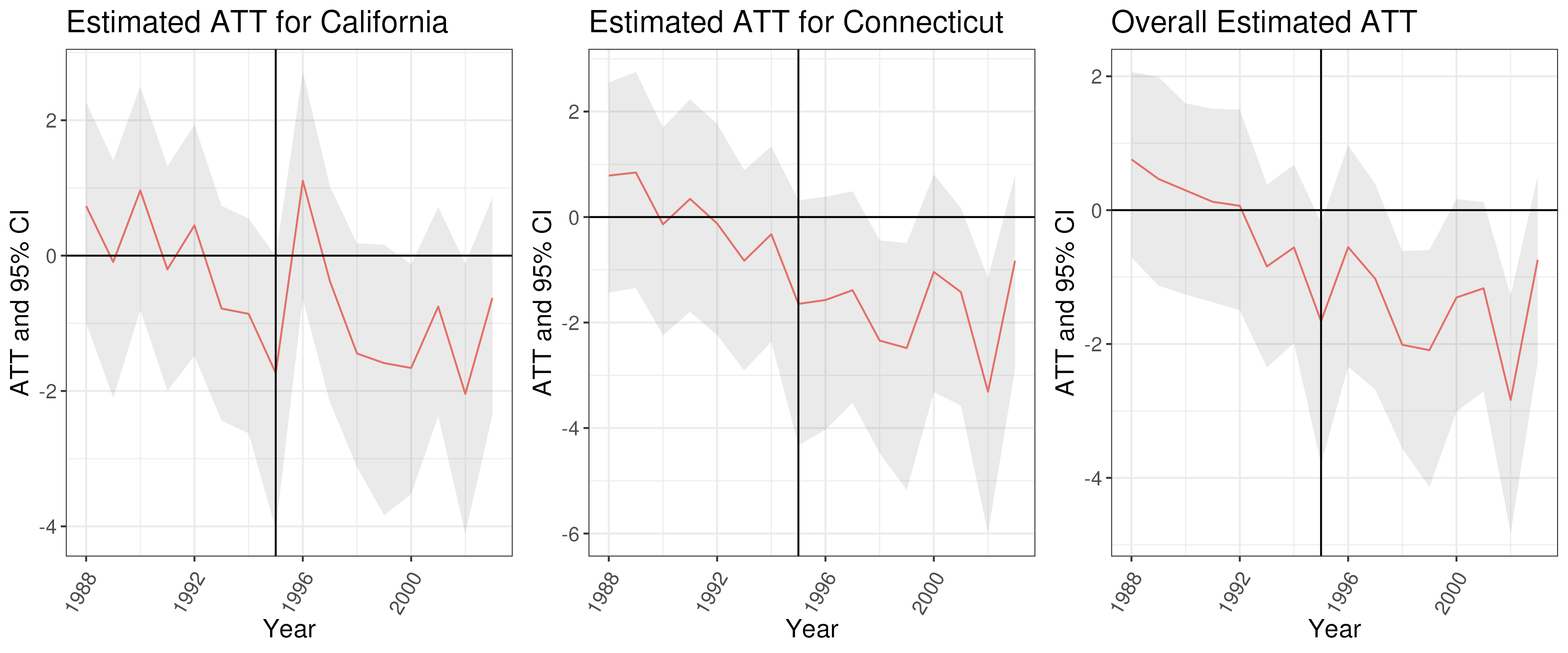
(a) Lymphoma

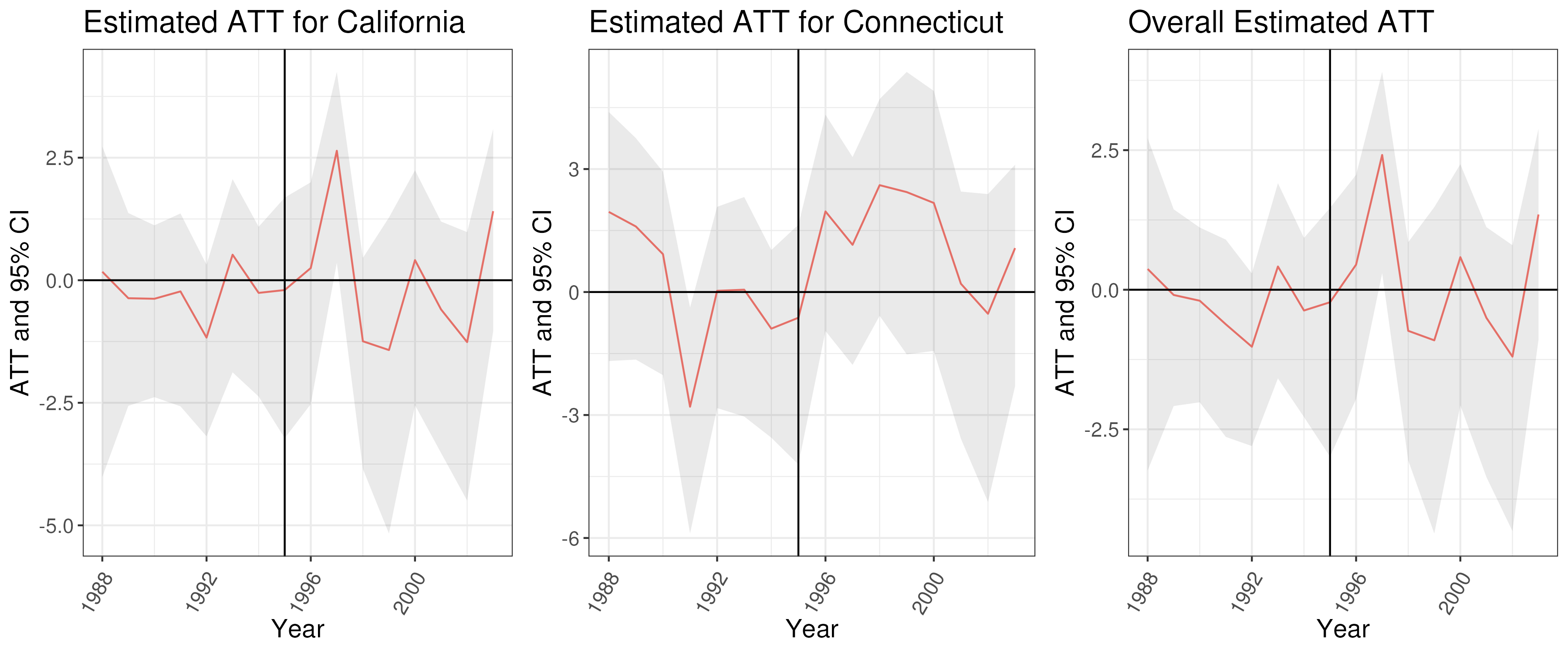
(b) Leukemia

Figure 2: Plots showing the estimated ATT over-time for incidence of lymphoma (a) and leukemia (b). The Space and Space-Time Lasso Models were chosen respectively based on evaluation of all models pre-treatment fits.

The reformulated gasoline program was first passed and announced in 1990, although it was not imposed in covered areas until 1995. However, prior research suggests that there was an anticipatory effect of the program on gasoline content and TRAP in covered areas, which may explain the declining lymphoma ATT estimates prior to treatment. Take for example benzene, which is a key traffic-related pollution that has been implicated in hematologic cancer development and one that was targeted for reduction in reformulated gasoline [1, 2]. In California, ambient benzene concentrations at monitoring sites was decreasing steadily during the period 1990-1994, prior to the formal implementation of the reformulated gasoline program, with a total decrease of about 40% during this pre-treatment period [10]. Although there are no benzene monitors in Connecticut, ambient benzene concentrations in nearby New York City began declining in 1990, although there was a clear, sharp decline between 1995 and 1996 [49]. It is possible that since ambient benzene (and possibly other traffic-related pollutants) began declining prior to the implementation of the reformulated gasoline program, any resulting health impacts might have begun to materialize prior to 1995.

Because of this possible anticipatory effect of the reformulated gasoline program, we conduct sensitivity analyses considering 1990 as the treated year, and expanding our study period to 1983-2003 to allow for adequate pre-treatment data for these analyses (Section S.2). The pre-treatment ATT estimates from these models are centered around zero and absent systematic temporal trends for both leukemia and lymphoma (Figure S2), indicating strong model fit for both diseases. However, the results are very similar to those in our main analyses, with identical conclusions about the effects of the reformulated gasoline program. Tables S4 - S5 show that the program led to decreases in lymphoma incidence, but results remain inconclusive for leukemia incidence.

We also conducted sensitivity analyses with increased $K$ ($K=3$ for Vanilla, Space, Space-Time ICAR, Space-Time AR, Space-Time Lasso, and Athey MC models and $K=4$ for the Space-Time Shrinkage model). Results are shown in Tables S9 and S10 and are similar to the results of our main analyses, indicating little sensitivity of our findings to choice to $K$.

5 Discussion

In this paper, we propose and evaluate causal inference approaches for studying the effects of a quasi-experiment on rare disease outcomes. Working within a Bayesian MC framework, we consider a number of prior distribution configurations to allow for spatio-temporal smoothing, regularization, and adaptive hyperparameter selection to reduce over-fitting and improve estimation in rare outcome contexts. The Bayesian approach also lends itself to more straightforward uncertainty quantification than its frequentist or machine learning counterparts [21]. Through our simulation study, we show that our proposed models perform better than numerous existing methods for quasi-experimental analysis in the context of rare disease outcomes. We find that both independent prior distributions and certain spatio-temporal priors on the MC latent factors and loadings perform well, and that over-specifying the unknown number of latent factors presents a greater threat to predictive accuracy than under-specifying when working with disease outcomes.

Building on the sparse infinite factor model framework of Bhattacharya and Dunson [43], we also introduce and implement prior distributions on the latent factors and factor loadings that can simultaneously perform spatio-temporal smoothing and adaptively select the number of latent factors. This eliminates the need for user-specification of $K$, which may reduce model sensitivity to arbitrary tuning parameter selection in real data applications. To our knowledge, such prior distributions have not yet been proposed in the MC literature. Our simulation studies showed that this approach consistently performed well, with results comparable to the best-performing models under user-specification of $K$.

In our real data analysis, we found evidence that the EPA’s reformulated gasoline program may have led to reductions in childhood and young adult lymphoma, but had no effect on childhood leukemia. These findings are consistent with the recent findings of Nethery et al. [50], who studied the effects of a separate, smaller-scale gasoline reformulation program implemented by the US EPA in Alaska in 2011. This program, known as the Mobile Source Air Toxics Rule, was specifically focused on limiting the amount of benzene in gasoline. Applying difference-in-differences methods, Nethery et al. also observed a reduction in childhood and young adult lymphoma incidence following the implementation of this program (but no impact on childhood leukemia incidence). While prior literature based on observational studies has primarily reported associations between TRAP exposure and childhood leukemia [3, 4, 5, 6], these recent findings of associations between TRAP and childhood lymphoma using more robust quasi-experimental study designs suggest that greater attention to this potential link is warranted.

A limitation of our work is that we do not have information about cross-county migration, which could induce exposure measurement error. For example, a person could develop leukemia or lymphoma while living in an unregulated county and then move to a regulated county where diagnosis occurs (or vice versa). Additionally, violations of the standard SUTVA assumptions for causal inference are possible in our real data application. For instance, SUTVA requires that there is only one "version" of treatment. Here, the intervention likely led to different degrees of change in exposure (likely larger decreases in TRAP exposure in urban areas vs. rural). However, because MC approaches do not model the outcomes under treatment (instead simply making use of the observed outcomes under treatment to estimate causal effects), we anticipate that any such issues would not affect our modeling and would only compel a more nuanced interpretation of the causal quantities being estimated. SUTVA also requires the “no interference” condition, i.e., that the treatment of one unit should not affect the potential outcomes of another unit. Violations of no interference could occur, for instance, if residents of unregulated areas commute regularly to nearby regulated areas and thereby reap the health benefits of the improved air quality in regulated areas. However, the structure of the reformulated gasoline program implementation and our SEER data are likely to mitigate this issue, as entire states are considered treated or untreated, and our data do not include any bordering states.

Given recent decreased focus on the development of federal environmental regulations in the US, individual cities and states have begun to make their own laws to decrease environmental exposures suspected to be harmful [51]. These localized environmental health regulations are ideal QEs and provide the opportunity to study the effects of many different contaminants on disease outcomes. The methods introduced here will enable robust analysis of the health impacts of these QEs, including impacts on rare disease outcomes.

Data and code availability

The cancer incidence data used here cannot be redistributed under the conditions of the Data Use Agreements. However, interested parties can request the data through the standard processes described on the SEER and California Cancer Registry websites. Code to reproduce all simulations and real data analyses is available at https://github.com/sofiavega98/trap_cancer_SpaceTimeMC/. The computations in this paper were run on the FASRC Cannon cluster supported by the FAS Division of Science Research Computing Group at Harvard University.

S Supplementary Materials

S.1 Simulation Studies with Alternative Prior Specification

Alternatively, we place a $\mathrm{Ga(1,0.01)}$ prior on $\tau^{2}$, $\tau_{S}^{2}$, and $\tau_{T}^{2}$ in the Space, Space-Time ICAR, Space-Time AR, and Space-Time Shrinkage Models as suggested by the default prior specification in the CARBayes R package [52]. Although this prior specification leads to fewer models diverging (Table: S.1), it increases absolute percent bias of the ATT in most cases (Table: S.1).

Table S1: Percent of Simulations Diverging

Model	K	Non-Rare & Non-Smoothed	Non-Rare & Smoothed	Rare & Non-Smoothed	Rare & Smoothed
Vanilla	1	0	0	0	0
	3	0	0	0	0
	7	0	0	0	0
Space	1	0	0	0	0
	3	0	0	0	0
	7	0	0	1	0
Space-Time ICAR	1	0	0	0	0
	3	0	0	0	0
	7	0	0	1	0
Space-Time AR	1	0	0	0	0
	3	0	0	0	0
	7	0	0	0	0
Space-Time Lasso	1	0	0	0	0
	3	0	0	0	0
	7	0	0	10	5
Space-Time Shrinkage	7	0	0	0	0

Table S2: Simulation results: Average absolute percent bias of the counterfactual estimates from each method applied with different specifications of the number of factors, $K$ (rows), in simulated data emulating rare and non-rare outcomes, with and without a temporal smoothing pre-processing step (columns).

Model	K	Non-Rare & Non-Smoothed	Non-Rare & Smoothed	Rare & Non-Smoothed	Rare & Smoothed
Bayesian MC Models
Vanilla	1	6.08	5.89	15.76	15.96
	3	6.12	6.04	15.70	16.06
	7	6.50	6.00	17.95	16.86
Space	1	6.20	6.35	17.70	16.98
	3	7.31	7.03	21.22	18.55
	7	8.66	7.95	29.97	29.73
Space-Time ICAR	1	6.32	6.15	18.07	15.40
	3	7.35	6.62	22.13	19.02
	7	10.28	9.27	31.65	28.02
Space-Time AR	1	5.74	5.87	14.92	15.73
	3	6.12	6.12	15.10	15.20
	7	6.22	6.56	16.96	17.36
Space-Time Lasso	1	6.10	5.78	17.31	16.31
	3	6.77	6.72	17.20	18.91
	7	7.55	7.56	23.16	22.11
Space-Time Shrinkage	7	6.31	6.22	16.96	16.85
Existing Methods
Athey MC	1	7.18	7.01	16.97	17.02
	3	7.04	6.96	17.18	17.32
	7	7.09	6.97	16.77	17.11
GSC	NA	7.04	7.05	19.01	16.98
ASC	NA	6.78	7.15	20.70	20.29

S.2 Real Data Sensitivity Analysis

Since ambient benzene began declining in 1990, we considered leukemia and lymphoma incidence data from 1983 to 2003 with 1990 as the treated year. Due to data access limitations, we used SEER incidence data for the both lymphoma and leukemia.

Figure S1 show preliminary principal component analyses for both data sets. With these results, $K=2$ chosen for the Vanilla, Space, Space-Time ICAR, Space-Time AR, Space-Time Lasso, and Athey MC Models and $K=3$ was chosen for the Space-Time Shrinkage Model.

We similarly run 2,000 Hamiltonian Monte Carlo iterations with 1,000 burn-in iterations in rstan for each of our models. Table S3 shows R-hat values for our models indicating proper convergence. Results are shown in Tables S4 and S5. Figure S2 shows the estimated ATT over time. Overall results agree with those shown in the Application Section (Section 4), but 1(a) shows improved pre-treatment trends for incidence of CYA lymphoma.

(c)

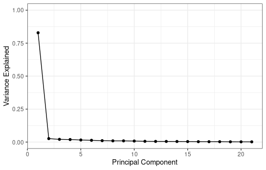
(d)

Figure S1: Scree plots showing the percent of variance explained by each principal component for each panel data matrix: lymphoma (a) and leukemia (b).

Table S3: Average R-hat for each model’s counterfactual predictions applied with different specifications of the number of factors, $K$ (rows), in CYA lymphoma and leukemia incidence data, with and without a temporal smoothing pre-processing step (columns).

Model	K	Lymphoma & Non-Smoothed	Lymphoma & Smoothed	Leukemia & Non-Smoothed	Leukemia & Smoothed
Vanilla	2	1.00	1.00	1.00	1.00
Space	2	1.01	1.03	1.04	1.02
Space-Time ICAR	2	1.01	1.05	1.02	1.02
Space-Time AR	2	1.04	1.01	1.01	1.02
Space-Time Lasso	2	1.02	1.03	1.02	1.03
Space-Time Shrinkage	3	1.02	1.02	1.02	1.01

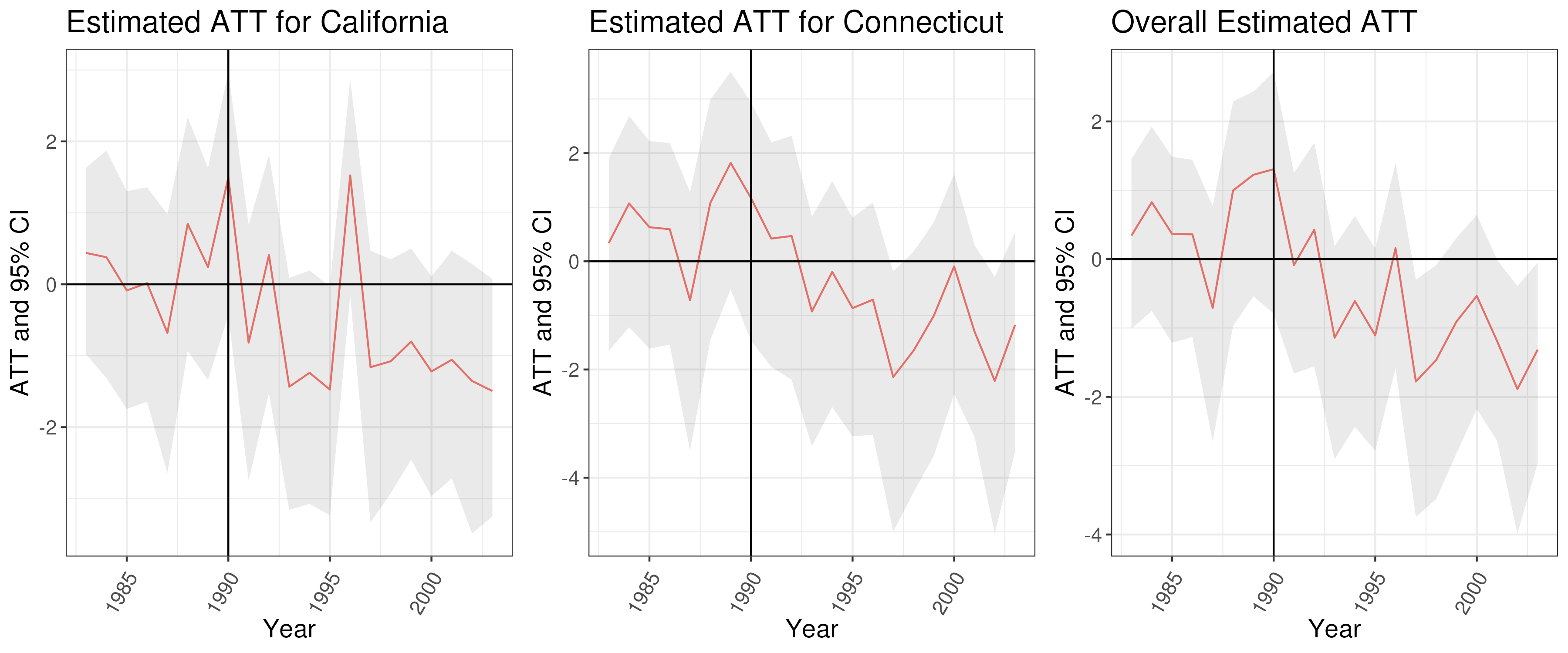
(a)

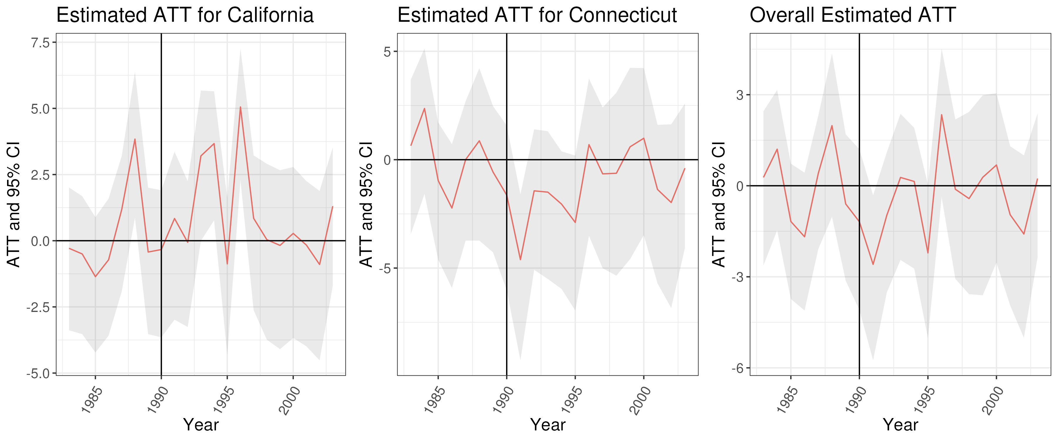
(b)

Figure S2: Plots showing the estimated ATT over-time for incidence of lymphoma (a) and leukemia (b) in the absence of temporal smoothing. The Space-Time AR Model was chosen based on the results of the simulation study.

Table S4: Overall and state-specific estimated ATT results for each model applied to CYA lymphoma and leukemia incidence data without a temporal smoothing pre-processing step.

Model	California		Connecticut		Overall
	ATT	95% CI	ATT	95% CI	ATT	95% CI
Lymphoma
Athey MC	-0.23	NA	-1.08	NA	-0.76	(-1.61 , 0.10)
Vanilla	-0.79	(-1.65 , 0.08)	-1.37	(-2.37 , -0.49)	-1.15	(-1.92 , -0.48)
Space	-0.56	(-1.41 , 0.10)	-1.37	(-2.36 , -0.53)	-1.09	(-1.83 , -0.43)
Space-Time ICAR	-0.76	(-1.57 , -0.09)	-1.53	(-2.45 , -0.57)	-1.24	(-1.95 , -0.56)
Space-Time AR	-0.70	(-1.45 , -0.20)	-0.66	(-2.18 , 0.06)	-0.68	(-1.73 , -0.17)
Space-Time Lasso	-0.75	(-1.52 , -0.11)	-1.15	(-2.16 , -0.31)	-1.01	(-1.73 , -0.38)
Space-Time Shrinkage	-0.74	(-1.73 , 0.14)	-1.45	(-2.40 , -0.61)	-1.18	(-1.87 , -0.56)
Leukemia
Athey MC	0.91	NA	-0.05	NA	0.32	(-1.07 , 1.71)
Vanilla	0.58	(-1.43 , 1.98)	-1.31	(-3.24 , 0.20)	-0.59	(-2.15 , 0.61)
Space	0.08	(-2.12 , 1.49)	-1.51	(-3.66 , -0.08)	-0.85	(-2.85 , 0.22)
Space-Time ICAR	0.46	(-0.79 , 1.94)	-1.93	(-3.93 , -0.22)	-1.04	(-2.40 , 0.36)
Space-Time AR	0.89	(-0.90 , 1.80)	-1.31	(-3.00 , 0.07)	-0.48	(-1.79 , 0.41)
Space-Time Lasso	-0.77	(-0.9 , 2.09)	-1.29	(-3.12 , 0.15)	-0.47	(-1.83 , 0.45)
Space-Time Shrinkage	0.76	(-1.84 , 0.35)	-0.38	(-1.31 , 0.47)	-0.52	(-1.24 , 0.09)

Table S5: Overall and state-specific estimated ATT results for each model applied to CYA lymphoma and leukemia incidence data with a temporal smoothing pre-processing step.

Model	California		Connecticut		Overall
	ATT	95% CI	ATT	95% CI	ATT	95% CI
Lymphoma
Athey MC	0.02	NA	-0.66	NA	-0.40	(-1.10 , 0.44)
Vanilla	-0.58	(-2.18 , 0.59)	-1.25	(-2.69 , -0.18)	-0.99	(-2.19 , -0.10)
Space	-0.54	(-1.29 , 0.11)	-1.27	(-2.05 , -0.59)	-0.97	(-1.63 , -0.50)
Space-Time ICAR	-0.31	(-1.36 , 0.60)	-0.35	(-1.54 , 0.70)	-0.37	(-1.06 , 0.51)
Space-Time AR	-0.62	(-1.36 , 0.09)	-1.16	(-2.06 , -0.32)	-0.94	(-1.63 , -0.35)
Space-Time Lasso	-0.62	(-0.30 , 1.51)	-1.06	(-2.25 , -0.08)	-0.38	(-1.15 , 0.25)
Space-Time Shrinkage	0.65	(-1.52 , 0.14)	-1.00	(-1.94 , -0.26)	-0.84	(-1.62 , -0.36)
Leukemia
Athey MC	1.37	NA	0.74	NA	0.98	(-0.41 , 2.54)
Vanilla	0.91	(-1.57 , 2.55)	-0.42	(-2.83 , 1.3)	0.05	(-1.67 , 1.3)
Space	-0.01	(-1.75 , 1.28)	-0.33	(-1.96 , 0.76)	-0.22	(-1.39 , 0.66)
Space-Time ICAR	0.17	(-1.45 , 1.57)	-0.41	(-1.72 , 0.81)	-0.21	(-1.26 , 0.86)
Space-Time AR	0.87	(-0.25 , 1.96)	-0.57	(-2.03 , 0.80)	0	(-1.07 , 0.95)
Space-Time Lasso	0.12	(-0.34 , 1.83)	-0.64	(-2.55 , 0.46)	-0.01	(-1.48 , 0.77)
Space-Time Shrinkage	1.01	(-1.19 , 1.25)	-1.41	(-3.19 , -0.22)	-0.84	(-1.82 , -0.02)

S.3 Additional Tables and Figures

Table S6: Counties included in the federal RFG program in 1995.

State	Counties
California	Los Angeles, Orange,
	Ventura, San Bernardino,
	Riverside, San Diego
Connecticut	Hartford, Middlesex,
	New Haven, New London,
	Tolland, Windham,
	Fairfield, Litchfield
New Jersey	Bergen, Essex,
	Hudson, Hunterdon,
	Middlesex, Monmouth,
	Morris, Ocean, Passaic
	Somerset, Sussex, Union
	Burlington, Camden,
	Cumberland, Gloucester,
	Mercer, Salem
New York	Bronx, Kings, Nassau,
	New York, Orange, Putnam,
	Queens, Richmond,
	Rockland, Suffolk,
	Westchester
Delaware	Kent, New Castle
Maryland	Cecil Anne Arundel,
	Baltimore, Carroll,
	Harford, Howard
Pennsylvania	Bucks, Chester, Delaware
	Montgomery, Philadelphia
Indiana	Lake, Porter
Texas	Brazoria, Chambers,
	Fort Bend, Galveston, Harris,
	Liberty, Montgomery, Waller
Wisconsin	Kenosha, Milwaukee,
	Ozaukee, Racine,
	Washington, Waukesha

Table S7: Percent of Simulations Diverging

Model	K	Non-Rare & Non-Smoothed	Non-Rare & Smoothed	Rare & Non-Smoothed	Rare & Smoothed
Vanilla	1	0	0	0	0
	3	0	0	0	0
	7	0	0	0	0
Space	1	0	0	0	0
	3	0	0	0	0
	7	0	0	12	8
Space-Time ICAR	1	0	0	0	0
	3	0	0	0	0
	7	0	0	16	7
Space-Time AR	1	0	0	0	0
	3	0	0	0	0
	7	0	0	0	0
Space-Time Lasso	1	0	0	0	0
	3	0	0	0	0
	7	0	0	10	5
Space-Time Shrinkage	7	0	0	0	0

(a)

(b)

Figure S3: Scree plots showing the percent of variance explained by each principal component for each panel data matrix: lymphoma (a) and leukemia (b).

Table S8: Average R-hat for each model’s counterfactual predictions applied with different specifications of the number of factors, $K$ (rows), in CYA lymphoma and leukemia incidence data, with and without a temporal smoothing pre-processing step (columns).

Model	K	Lymphoma & Non-Smoothed	Lymphoma & Smoothed	Leukemia & Non-Smoothed	Leukemia & Smoothed
Vanilla	2	1.01	1.00	1.00	1.00
	3	1.01	1.00	1.00	1.00
Space	2	1.02	1.02	1.02	1.02
	3	1.02	1.02	1.02	1.03
Space-Time ICAR	2	1.02	1.02	1.02	1.02
	3	1.03	1.04	1.05	1.03
Space-Time AR	2	1.01	1.01	1.04	1.02
	3	1.01	1.01	1.01	1.02
Space-Time Lasso	2	1.02	1.02	1.01	1.02
	3	1.02	1.05	1.03	1.02
Space-Time Shrinkage	3	1.01	1.03	1.02	1.03
	4	1.03	1.01	1.01	1.02

Table S9: Overall and state-specific estimated ATT results for each model applied with different specifications of the number of factors, $K$ (rows), in CYA lymphoma and leukemia incidence data with a temporal smoothing pre-processing step.

Model	K	California		Connecticut		Overall
		ATT	95% CI	ATT	95% CI	ATT	95% CI
Lymphoma
Athey MC	2	-0.36	NA	-1.42	NA	-1.01	(-2.10 , 0.05)
	3	-0.36	NA	-1.42	NA	-1.01	(-2.11 , 0.05)
Vanilla	2	-0.80	(-2.40 , 0.42)	-1.66	(-3.36 , -0.37)	-1.33	(-2.75 , -0.26)
	3	-1.02	(-2.66 , 0.37)	-1.74	(-3.40 , -0.43)	-1.47	(-2.83 , -0.43)
Space	2	0.14	(-0.60 , 1.29)	-1.68	(-2.71 , -0.77)	-0.97	(-1.63 , -0.26)
	3	-0.21	(-1.13 , 0.36)	-1.45	(-2.45 , -0.55)	-1.00	(-1.69 , -0.35)
Space-Time ICAR	2	-1.14	(-2.18 , -0.49)	-1.04	(-2.03 , -0.27)	-1.08	(-1.88 , -0.55)
	3	-0.52	(-2.33 , 0.22)	-1.53	(-3.45 , -0.64)	-1.15	(-2.90 , -0.46)
Space-Time AR	2	-0.89	(-1.69 , -0.08)	-1.70	(-2.59 , -0.73)	-1.38	(-2.10 , -0.60)
	3	-0.79	(-1.59 , -0.07)	-1.48	(-2.61 , -0.59)	-1.21	(-1.97 , -0.53)
Space-Time Lasso	2	-0.72	(-1.92 , 0.05)	-1.63	(-2.63 , -0.69)	-1.34	(-2.22 , -0.62)
	3	-0.65	(-1.87 , 0.46)	-0.38	(-2.04 , 0.56)	-0.30	(-1.81 , 0.39)
Space-Time Shrinkage	3	-0.84	(-1.34 , -0.08)	-1.23	(-1.93 , -0.59)	-1.04	(-1.57 , -0.53)
	4	-0.25	(-1.20 , -0.12)	-1.49	(-2.15 , -0.87)	-1.17	(-1.64 , -0.75)
Leukemia
Athey MC	2	-1.12	NA	0.88	NA	-0.85	(-3.60 , 1.40)
	3	-1.11	NA	0.89	NA	-0.84	(-3.79 , 1.60)
Vanilla	2	0.16	(-1.02 , 1.12)	0.79	(-1.50 , 2.18)	0.24	(-0.92 , 1.12)
	3	0.13	(-1.05 , 1.04)	0.62	(-1.64 , 2.19)	0.20	(-0.95 , 1.05)
Space	2	0.15	(-1.03 , 1.02)	1.10	(-0.52 , 2.34)	0.30	(-0.77 , 1.02)
	3	-1.26	(-14.10 , 0.12)	-1.04	(-5.37 , 1.08)	-1.33	(-12.26 , 0.06)
Space-Time ICAR	2	0.19	(-1.35 , 0.96)	1.23	(-0.30 , 2.29)	0.32	(-1.00 , 1.02)
	3	-0.65	(-2.74 , 0.51)	0.89	(-6.57 , 2.35)	-0.51	(-2.83 , 0.46)
Space-Time AR	2	0.28	(-0.72 , 0.99)	-0.28	(-2.68 , 1.37)	0.20	(-0.73 , 0.87)
	3	0.43	(-0.42 , 1.23)	1.14	(-0.47 , 2.52)	0.50	(-0.26 , 1.24)
Space-Time Lasso	2	0.42	(-1.74 , 0.96)	1.13	(-0.45 , 2.33)	-0.05	(-1.37 , 1.01)
	3	-0.15	(-1.57 , 0.97)	-1.71	(-6.78 , 0.87)	-0.39	(-1.83 , 0.81)
Space-Time Shrinkage	3	-0.24	(-0.67 , 1.16)	1.28	(0.04 , 2.54)	0.53	(-0.46 , 1.27)
	4	-0.15	(-0.45 , 1.29)	0.88	(-2.10 , 2.19)	0.57	(-0.35 , 1.27)

Table S10: Overall and state-specific estimated ATT results for each model applied with different specifications of the number of factors, $K$ (rows), in CYA lymphoma and leukemia incidence data without a temporal smoothing pre-processing step.

Model	K	California		Connecticut		Overall
		ATT	95% CI	ATT	95% CI	ATT	95% CI
Lymphoma
Athey MC	3	-0.46	NA	-1.60	NA	-1.16	(-2.19 , -0.13)
Vanilla	3	-0.95	(-2.08 , -0.01)	-1.64	(-2.89 , -0.54)	-1.38	(-2.33 , -0.58)
Space	3	-0.77	(-1.62 , -0.06)	-1.72	(-2.81 , -0.87)	-1.37	(-2.04 , -0.79)
Space-Time ICAR	3	-0.59	(-1.22 , -0.06)	-1.38	(-2.95 , -0.65)	-1.08	(-2.08 , -0.59)
Space-Time AR	3	-0.77	(-1.67 , 0.02)	-1.56	(-2.58 , -0.71)	-1.27	(-1.95 , -0.60)
Space-Time Lasso	3	-0.93	(-1.41 , 0.23)	-2.03	(-3.00 , -1.18)	-1.43	(-2.14 , -0.85)
Space-Time Shrinkage	4	-0.41	(-1.61 , -0.31)	-1.54	(-2.30 , -0.88)	-1.31	(-1.80 , -0.86)
Leukemia
Athey MC	3	-1.60	NA	0.72	NA	-1.29	(-3.87 , 1.30)
Vanilla	3	-0.21	(-1.41 , 0.91)	0.69	(-1.14 , 2.24)	-0.09	(-1.18 , 0.94)
Space	3	-0.66	(-17.85 , 0.53)	1.14	(-0.22 , 2.42)	-0.45	(-15.41 , 0.61)
Space-Time ICAR	3	-0.99	(-3.32 , 0.41)	0.50	(-0.95 , 1.89)	-0.81	(-2.81 , 0.48)
Space-Time AR	3	-0.17	(-1.32 , 0.79)	0.69	(-0.91 , 1.91)	-0.06	(-1.07 , 0.78)
Space-Time Lasso	3	0.13	(-3.10 , 0.84)	0.32	(-4.37 , 2.14)	-0.08	(-2.99 , 0.86)
Space-Time Shrinkage	4	-0.12	(-0.98 , 0.98)	0.91	(-0.75 , 2.30)	0.21	(-0.72 , 1.03)

References

- [1] Robert A Rinsky, Ronald J Young, and Alexander B Smith. Leukemia in benzene workers. American Journal of Industrial Medicine, 2(3):217–245, 1981.
- [2] Robert A Rinsky, Alexander B Smith, Richard Hornung, Thomas G Filloon, Ronald J Young, Andrea H Okun, and Philip J Landrigan. Benzene and leukemia. New England journal of medicine, 316(17):1044–1050, 1987.
- [3] Ole Raaschou-Nielsen and Peggy Reynolds. Air pollution and childhood cancer: A review of the epidemiological literature. International journal of cancer, 118(12):2920–2929, 2006.
- [4] Vickie L Boothe, Tegan K Boehmer, Arthur M Wendel, and Fuyuen Y Yip. Residential traffic exposure and childhood leukemia: A systematic review and meta-analysis. American Journal of Preventive Medicine, 46(4):413–422, 2014.
- [5] Xiao-Xi Sun, Shan-Shan Zhang, and Xiao-Ling Ma. No association between traffic density and risk of childhood leukemia: A meta-analysis. Asian Pacific Journal of Cancer Prevention, 15(13):5229–5232, 2014.
- [6] Tommaso Filippini, Julia E Heck, Carlotta Malagoli, Cinzia Del Giovane, and Marco Vinceti. A review and meta-analysis of outdoor air pollution and risk of childhood leukemia. Journal of Environmental Science and Health, Part C, 33(1):36–66, 2015.
- [7] Patricia A Buffler, Marilyn L Kwan, Peggy Reynolds, and Kevin Y Urayama. Environmental and genetic risk factors for childhood leukemia: Appraising the evidence. Cancer Investigation, 23(1):60–75, 2005.
- [8] Martha S Linet. Etiology of childhood leukemia: Environment, genes, controversies, and conundrums, 2005.
- [9] Maximilian Auffhammer and Ryan Kellogg. Clearing the air? the effects of gasoline content regulation on air quality. American Economic Review, 101(6):2687–2722, 2011.
- [10] Ralph Propper, Patrick Wong, Son Bui, Jeff Austin, William Vance, Alvaro Alvarado, Bart Croes, and Dongmin Luo. Ambient and emission trends of toxic air contaminants in California. Environmental Science & Technology, 49(19):11329–11339, 2015.
- [11] Robert A Harley, Daniel S Hooper, Andrew J Kean, Thomas W Kirchstetter, James M Hesson, Nancy T Balberan, Eric D Stevenson, and Gary R Kendall. Effects of reformulated gasoline and motor vehicle fleet turnover on emissions and ambient concentrations of benzene. Environmental Science & Technology, 40(16):5084–5088, 2006.
- [12] Alberto Abadie, Alexis Diamond, and Jens Hainmueller. Synthetic control methods for comparative case studies: Estimating the effect of California’s tobacco control program. Journal of the American Statistical Association, 105(490):493–505, 2010.
- [13] Dmitry Arkhangelsky, Guido W Imbens, Lihua Lei, and Xiaoman Luo. Double-robust two-way-fixed-effects regression for panel data. arXiv preprint arXiv:2107.13737, 2021.
- [14] Dmitry Arkhangelsky, Susan Athey, David A Hirshberg, Guido W Imbens, and Stefan Wager. Synthetic difference-in-differences. American Economic Review, 111(12):4088–4118, 2021.
- [15] Eli Ben-Michael, Avi Feller, and Jesse Rothstein. The augmented synthetic control method. Journal of the American Statistical Association, 116(536):1789–1803, 2021.
- [16] Susan Athey, Mohsen Bayati, Nikolay Doudchenko, Guido Imbens, and Khashayar Khosravi. Matrix completion methods for causal panel data models. Journal of the American Statistical Association, 116(536):1716–1730, 2021.
- [17] Yiqing Xu. Generalized synthetic control method: Causal inference with interactive fixed effects models. Political Analysis, 25(1):57–76, 2017.
- [18] Jinyong Hahn and Ruoyao Shi. Synthetic Control and Inference. Econometrics, 5(4):1–12, November 2017.
- [19] Victor Chernozhukov, Kaspar Wüthrich, and Yinchu Zhu. An exact and robust conformal inference method for counterfactual and synthetic controls. Journal of the American Statistical Association, 116(536):1849–1864, 2021.
- [20] Xun Pang and Licheng Liu. A bayesian multifactor spatio-temporal model for estimating time-varying network interdependence. Available at SSRN 3792628, 2021.
- [21] Masahiro Tanaka. Bayesian matrix completion approach to causal inference with panel data. Journal of Statistical Theory and Practice, 15(2):1–22, 2021.
- [22] Rachel C Nethery, Nina Katz-Christy, Marianthi-Anna Kioumourtzoglou, Robbie M Parks, Andrea Schumacher, and G Brooke Anderson. Integrated causal-predictive machine learning models for tropical cyclone epidemiology. Biostatistics, page kxab047, 2021.
- [23] US EPA O. Reformulated Gasoline. US EPA. https://www.epa.gov/gasoline-standards/reformulated-gasoline Published August 7, 2015.
- [24] National Research Council and others. Ozone-forming potential of reformulated gasoline. National Academies Press, 1999.
- [25] Surveillance, Epidemiology, and End Results (SEER) Program. SEER*Stat Database: Incidence - SEER Research Data, 8 Registries, Nov 2021 Sub (1975-2020) - Linked To County Attributes - Time Dependent (1990-2020) Income/Rurality, 1969-2020 Counties, National Cancer Institute, DCCPS, Surveillance Research Program, released April 2023, based on the November 2022 submission. www.seer.cancer.gov.
- [26] Graça M Dores, Susan S Devesa, Rochelle E Curtis, Martha S Linet, and Lindsay M Morton. Acute leukemia incidence and patient survival among children and adults in the United States, 2001-2007. Blood, The Journal of the American Society of Hematology, 119(1):34–43, 2012.
- [27] Jennifer F Yamamoto and Marc T Goodman. Patterns of leukemia incidence in the United States by subtype and demographic characteristics, 1997–2002. Cancer Causes & Control, 19:379–390, 2008.
- [28] U.S. Cancer Statistics Working Group. U.S. Cancer Statistics Data Visualizations Tool, based on 2021 submission data (1999-2019): U.S. Department of Health and Human Services, Centers for Disease Control and Prevention and National Cancer Institute, 2022.
- [29] Todd P Whitehead, Catherine Metayer, Joseph L Wiemels, Amanda W Singer, and Mark D Miller. Childhood leukemia and primary prevention. Current Problems in Pediatric and Adolescent Health Care, 46(10):317–352, 2016.
- [30] Donald B. Rubin. Estimating causal effects of treatments in randomized and nonrandomized studies. Journal of Educational Psychology, 66(5):688–701, October 1974.
- [31] Donald B Rubin. Randomization analysis of experimental data: The Fisher randomization test comment. Journal of the American Statistical Association, 75(371):591–593, 1980.
- [32] Ruslan Salakhutdinov and Andriy Mnih. Bayesian probabilistic matrix factorization using Markov chain Monte Carlo. In Proceedings of the 25th international conference on Machine learning, pages 880–887, 2008.
- [33] Ali Taylan Cemgil. Bayesian inference for nonnegative matrix factorisation models. Computational Intelligence and Neuroscience, 2009, 2009.
- [34] Prem K Gopalan, Laurent Charlin, and David Blei. Content-based recommendations with poisson factorization. Advances in Neural Information Processing Systems, 27, 2014.
- [35] Dawen Liang, John W Paisley, Dan Ellis, et al. Codebook-based Scalable Music Tagging with Poisson Matrix Factorization. In ISMIR, pages 167–172, 2014.
- [36] Stan Development Team. RStan: the R interface to Stan, 2022. R package version 2.21.5.
- [37] Julian Besag and Charles Kooperberg. On conditional and intrinsic autoregressions. Biometrika, 82(4):733–746, 1995.
- [38] Robert F Engle. Autoregressive conditional heteroscedasticity with estimates of the variance of United Kingdom inflation. Econometrica: Journal of the Econometric Society, pages 987–1007, 1982.
- [39] Craig Anderson and Louise M Ryan. A comparison of spatio-temporal disease mapping approaches including an application to ischaemic heart disease in New South Wales, Australia. International Journal of Environmental Research and Public Health, 14(2):146, 2017.
- [40] Nicola G Best, Richard A Arnold, Andrew Thomas, Lance A Waller, and Erin M Conlon. Bayesian models for spatially correlated disease and exposure data. Bayesian Statistics, 6:131–156, 1999.
- [41] Ryo Masuda and Ryo Inoue. Point event cluster detection via the bayesian generalized fused lasso. ISPRS International Journal of Geo-Information, 11(3):187, 2022.
- [42] George Casella, Malay Ghosh, Jeff Gill, and Minjung Kyung. Penalized regression, standard errors, and Bayesian lassos. Bayesian Analysis, 5(2):369–411, 2010.
- [43] Anirban Bhattacharya and David B Dunson. Sparse Bayesian infinite factor models. Biometrika, pages 291–306, 2011.
- [44] Lukas Snoek. NI-edu Online Course, 2021. https://lukas-snoek.com/NI-edu/index.html.
- [45] Yiqing Xu and Licheng Liu. gsynth: Generalized Synthetic Control Method, 2022. R package version 1.2.1.
- [46] Jesse Rothstein Eli Ben-Michael, Avi Feller. augsynth: Augmented Synthetic Control Method, 2018. R package version 1.2.1.
- [47] Brian G Leroux, Xingye Lei, and Norman Breslow. Estimation of disease rates in small areas: A new mixed model for spatial dependence. In Statistical Models in Epidemiology, the Environment, and Clinical trials, pages 179–191. Springer, 2000.
- [48] Aki Vehtari, Andrew Gelman, Daniel Simpson, Bob Carpenter, and Paul-Christian Bürkner. Rank-normalization, folding, and localization: An improved R for assessing convergence of MCMC (with discussion). Bayesian Analysis, 16(2):667–718, 2021.
- [49] Nenad Aleksic, Garry Boynton, Gopal Sistla, and Jacqueline Perry. Concentrations and trends of benzene in ambient air over New York State during 1990–2003. Atmospheric Environment, 39(40):7894–7905, 2005.
- [50] Rachel C Nethery, Sofia Vega, A Lindsay Frazier, and Francine Laden. Mobile source benzene regulations and risk of childhood and young adult hematologic cancers in Alaska: A quasi-experimental study. Epidemiology, pages 10–1097, 2022.
- [51] Safe States. Bill Tracker. https://www.saferstates.com/bill-tracker/. Accessed July 11, 2023.
- [52] Duncan Lee. CARBayes: An R package for Bayesian spatial modeling with conditional autoregressive priors. Journal of Statistical Software, 55(13):1–24, 2013.