Abstract

Future zero-touch artificial intelligence (AI)-driven 6G network automation requires building trust in the AI black boxes via explainable artificial intelligence (XAI), where it is expected that AI faithfulness would be a quantifiable service-level agreement (SLA) metric along with telecommunications key performance indicators (KPIs). This entails exploiting the XAI outputs to generate transparent and unbiased deep neural networks (DNNs). Motivated by closed-loop (CL) automation and explanation-guided learning (EGL), we design an explanation-guided federated learning (EGFL) scheme to ensure trustworthy predictions by exploiting the model explanation emanating from XAI strategies during the training run time via Jensen-Shannon (JS) divergence. Specifically, we predict per-slice RAN dropped traffic probability to exemplify the proposed concept while respecting fairness goals formulated in terms of the recall metric which is included as a constraint in the optimization task. Finally, the comprehensiveness score is adopted to measure and validate the faithfulness of the explanations quantitatively. Simulation results show that the proposed EGFL-JS scheme has achieved more than $50\%$ increase in terms of comprehensiveness compared to different baselines from the literature, especially the variant EGFL-KL that is based on the Kullback-Leibler Divergence. It has also improved the recall score with more than $25\%$ relatively to unconstrained-EGFL.

I Introduction

Future 6G networks are expected to be a machine-centric technology, wherein all the corresponding smart things would operate intelligently yet as smart black boxes [1] that lack transparency in their prediction or decision-making processes and could have adverse effects on the 6G network’s operations. In this concern, XAI provides human interpretable methods to adequately explain the AI system and its predictions/decisions and gain the human’s trust in the loop, which is anticipated to be a quantifiable KPI [2] in future 6G networks. Nonetheless, most of the research on XAI for deep neural networks (DNNs) focuses mainly on generating explanations, e.g., in terms of feature importance or local model approximation in a post-hoc way that does not bridge the trade-off that exists between explainability and AI model’s performance [3] nor guarantee the predefined 6G trust KPI requirement. In this regard, there is less contribution on aspects related to the exploitation of the explanations during training, i.e. in an in-hoc fashion, which would orient the model towards yielding explainable outputs that fulfill a predefined trust level in AI-driven automated 6G networks, as well as tackling the explainability-performance trade-off [4]. This approach is called explanation-guided learning (EGL) [5, 6], which focuses on addressing the accuracy of prediction and explanation jointly, and their mutual relation in run-time. It is particularly relevant in the context of 6G, where the complexity of the network and the diversity of the applications being served make it essential to guarantee the target trust in AI-driven zero-touch management. This paper aims to present a distinct approach for improving federated learning models’ interpretability by introducing a new closed-loop training procedure that natively optimizes explainability and fairness goals along with the main use-case task of traffic drop probability prediction for 6G network slices.

I-A Related Works

In this section, we exhibit the state of the art of EGL to recognize interdisciplinary open research opportunities in this domain. Indeed, the works on EGL techniques are still in the early stage and facing technical challenges in developing their frameworks [7]. According to current studies, incorporating an additional explanation objective could potentially enhance the usefulness of DNNs in various application domains, including computer vision (CV) and natural language processing (NLP). However, its potential benefits for future 6G networks have not been thoroughly investigated yet. Despite this limited exploration, some researchers have started implementing XAI techniques to address telecommunication issues in this field. In particular, the authors of [8, 9] stress the importance of explainability and identify challenges associated with developing XAI methods in this domain. Additionally, the utilization of XAI for identifying the actual cause of Service Level Agreement (SLA) violations has been studied in [10]. Meanwhile, in [11, 12], the authors mention the necessity of XAI in the zero-touch service management (ZSM) autonomous systems and present a neuro-symbolic XAI twin framework for zero-touch management of Internet of Everything (IoE) services in the wireless network. Moreover, [13] emphasizes the utilization of the Federated Learning (FL) approach with XAI in 5G/6G networks. In [7], two types of EGL termed global guidance and local guidance explanation are mentioned, where both types refine the model’s overall decision-making process. Another line of work [14] introduces the EGL framework that allows the user to correct incorrect instances by creating simple rules capturing the target model’s prediction and retraining the model on that knowledge. While the authors of [15] define a very generic explanation-guided learning loss called Right for the Right Reasons loss (RRR). In addition, an approach to optimize model’s prediction and explanation jointly by enforcing whole graph regularization and weak supervision on model explanation is presented in [16]. Additionally, a novel training approach for existing few-shot classification models is presented in [17], which uses explanation scores from intermediate feature maps. Specifically, it leverages an adapted layer-wise relevance propagation (LRP) method and a model-agnostic explanation-guided training strategy to improve model’s generalization. So it is apparent that none of the aforementioned works has considered EGL in telecommunication domains for prediction and decision-making.

On the other hand, AI-native zero-touch network slicing automation has been introduced to govern the distributed nature of datasets [18] of various technological domains. Thus, a decentralized learning approach like federated learning (FL) [8] has gained attraction for fulfilling the beyond 5G network requirement. In this context, the authors of [19] proposed a method for dynamic resource allocation in decentralized RAN slicing using statistical FL. This approach enables effective resource allocation, SLA enforcement, and reduced communication overhead. However, the lack of a clear understanding of the underlying mechanisms in the paper may raise concerns about the trust and transparency of the proposed model.

Table I: Notations

Notation	Description
$S_{\mu}(\cdot)$	Logistic function with steepness $\mu$
$L$	Number of local epochs
$T$	Number of FL rounds
$\mathcal{D}_{k,n}$	Dataset at CL $(k,n)$
$D_{k,n}$	Dataset size
$\ell(\cdot)$	Loss function
$\mathbf{W}_{k,n}^{(t)}$	Local weights of CL $(k,n)$ at round $t$
$\mathbf{x}_{k,n}^{(i)}$	Input features
$\mathbf{y}_{k,n}^{(i)}$	Actual Output
$\hat{y}_{k,n}^{(i)}$	Predicted Output
$\gamma_{n}$	Recall lower-bound for slice $n$
$\tilde{x}_{k,n}^{(i)}$	Masked input features
$\tilde{p}_{k,n}^{(i)}$	Masked predictions
$\mathcal{D}_{k,n}$	Samples whose prediction fulfills the SLA
$\pi_{k,n}^{(i,j)}$	Probability Distribution
$\rho_{k,n}$	Recall Score
$\alpha_{k,n}^{(i,j)}$	Weighted attribution of features
$\mathbf{JS}_{k,n}$	Jensen Shannon Divergence
$\lambda_{(\cdot)}$	Lagrange multipliers
$R_{\lambda}$	Lagrange multiplier radius
$\mathcal{L}_{(\cdot)}$	Lagrangian with respect to ($\cdot$)

From this state-of-the-art (SoA) review, it turns out that incorporating FL and EGL strategies jointly can embrace into the network slicing of 6G RAN to address the absence of a trustworthy and interpretable solution in the prediction and decision-making process during learning. In this paper, we present the following contributions:

• To achieve transparent zero-touch service management of 6G network slices at RAN in a non-IID setup, a novel iterative explanation-guided federated learning approach is proposed, which leverages Jensen-Shannon divergence.

• A constrained traffic drop prediction model and integrated-gradient based explainer exchange attributions of the features and predictions in a closed loop way to predict per-slice RAN dropped traffic probability while respecting fairness constraints formulated in terms of recall. By demonstrating the traffic drop probability distribution and correlation heatmaps, we showcase the guided XAI’s potential to support decision-making tasks in the telecom industry.

• We frame the abovementioned fair sensitivity-aware constrained FL optimization problem under the proxy-Lagrangian framework and solve it via a non-zero sum two-player game strategy [20] and we show the comparison with state-of-the-art solutions, especially the EGFL-KL. Further, to assess the effectiveness of the proposed one, we report the recall and comprehensiveness performance, which provides a quantitative measure of the sensitivity and EGFL explanation level.

• More specifically, during the optimization process, we introduce a new federated EGL loss function that encompasses Jensen Shannon divergence to enhance model reliability and we also provide the corresponding results. We carefully scrutinize the normalized loss over the no. of FL rounds of the proposed EGFL model in the optimization process to support this phenomenon.

I-B Notations

We summarize the notations used throughout the paper in Table I.

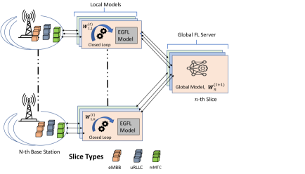
Figure 1: Federated traffic drop probability prediction in 6G RAN NS.

II Explanation Guided Learning Concept

As mentioned before, the leading goal of EGL is to enhance both the model performance as well as interpretability by jointly optimizing model prediction as well as the explanation during the learning process. So, the main objective function of Explanation-Guided Learning is defined in the existing research work of [7, 21], which is as follows:

$$\begin{split}&\min\,\underbrace{\mathcal{L}_{Pred}\left(\mathcal{F}\left(\mathcal{X}\right),\mathcal{Y}\right)}_{prediction}+\underbrace{\alpha\mathcal{L}_{Exp}\left({g}\left(\mathcal{F},\left(\mathcal{X,Y}\right)\right),\hat{M}\right)}_{explanation}\\ &+\underbrace{\beta\ohm\left({g}\left(\mathcal{F},\left(\mathcal{X,Y}\right)\right)\right)}_{regularization},\end{split}$$ (1)

From equation (1), we can observe three terms in the objective function of EGL. Where the first term defines the prediction loss of the model, the second term deals with the supervision of model explanation considering some explicit knowledge, and the last term can introduce some properties for achieving the right reason. These three terms can be specified and enforced differently, pivoting on each explanation-guided learning method [7]. However, it is noteworthy that we will adopt gradient based methods to explain the model’s prediction in our proposed work. It generates attributions by computing the gradient of the model’s output for its inputs, which indicates the input feature contributions to the model’s final prediction. Theoretically, the gradient values of all unimportant features should be close to zero, which may not hold in some complex situations, giving biased results in the model decision that is unexpected in the actual scenario [5]. So, even if we introduce explainability during the learning process of any AI system for some prediction or decision-making purpose, there is still a chance we will get a final decision that is biased or different from actual results. Additionally, this may hinder telecommunication service providers/operators from making their system transparent, only considering XAI. Considering the above fact and inspired by EGL, we came out with a solution to overcome this situation. We aim to introduce EGL to our proposed framework of 6G RAN network slicing during learning, ensuring that the irrelevant gradient will close to zero without sacrificing the model performance.

Table II: Dataset Features and Output

Feature	Description
Averege PRB	Average Physical Resource Block
Latency	Average transmission latency
Channel Quality	SNR value expressing the wireless channel quality
Output	Description
Dropped Traffic	Probability of dropped traffics (%)

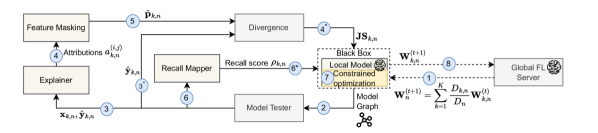
Figure 2: Explanation Guided FL building blocks

III RAN Architecture and Datasets

A shown in Fig. 1, we consider a radio access network (RAN), which is composed of a set of $K$ the base station (BSs), wherein a set of $N$ parallel slices are deployed, driven by the concept of slicing-enabled mobile networks [22]. The deployment of these parallel slices within the RAN enables efficient resource allocation, differentiation of services, and flexibility to meet diverse user and application needs. Here, each BS runs a local control closed-loop (CL) which collects monitoring data and performs traffic drop prediction. The local control CL system proactively manages network resources by gathering real-time data on network conditions and using predictive algorithms to estimate the likelihood of traffic drops or disruptions. Specifically, the collected data serves to build local datasets for slice $n\,(n=1,\ldots,N)$, i.e., $\mathcal{D}_{k,n}=\{\mathbf{x}_{k,n}^{(i)},y_{k,n}^{(i)}\}_{i=1}^{D_{k,n}}$, where $\mathbf{x}_{k,n}^{(i)}$ stands for the input features vector while $y_{k,n}^{(i)}$ represents the corresponding output. In this respect, Table II summarizes the features and the output of the local datasets. These accumulated datasets are non-IID due to the different traffic profiles induced by the heterogeneous users’ distribution and channel conditions. Moreover, since the collected datasets are generally non-exhaustive to train accurate anomaly detection classifiers, the local CLs take part in a federated learning task wherein an E2E slice-level federation layer plays the role of a model aggregator. In more specifics, each slice within the BS represents a diverse use case of vertical applications and is characterized by input features such as PRBs, channel quality, and latency. By leveraging these input features, the FL optimization process can train a predictive model guided by XAI that learns to predict the occurrence of traffic drops for each slice within the BS. This enables proactive measures to be taken to mitigate potential disruptions and optimize the performance of the communication system.

IV Explanation-Guided FL for Transparent Traffic Drop Prediction

In this section, we describe the different stages of the explanation-guided fair FL as summarized in Fig. 2.

IV-A Closed-Loop Description

In our proposed architecture, Fig. 2 represents a block that is placed within the local models shown in Fig. 1. This block is designed to facilitate proposed explainable guided federated learning, which involves iterative local learning with runtime explanation in a closed-loop manner. We design a simple neural network FL model. For each local epoch, the Learner module feeds the posterior symbolic model graph to the Tester block which yields the test features and the corresponding predictions $\hat{y}_{k,n}^{(i)}$ to the Explainer. The latter first generates the features attributions using integrated gradients XAI method.

The Featuere Masking block then selects, for each sample, the feature with lowest attribution and masks it. The corresponding masked inputs, $\tilde{x}_{k,n}^{(i)},(i=1,\ldots,D_{k,n})$ are afterward used to calculate the masked predictions, $\tilde{p}_{k,n}^{(i)},(i=1,\ldots,D_{k,n})$ that is fed back to the Divergence module at step 5. At the same time, predictions $\hat{y}_{k,n}^{(i)}$ from the tester block are fed in the Divergence block as shown in the step 3". Divergence module is the responsible to calculate Jensen-Shannon divergence between model predictions of original and masked inputs, $\mathbf{JS}(\hat{y}_{k,n}^{(i)}||\tilde{p}_{k,n}^{(i)})$. The corresponding result, denoted as $\mathbf{JS}_{k,n}$ from this module is included with cross entropy loss as the objective function of the local model, shown at the stage 4". Similarly, the Recall Mapper calculates the recall score $\rho_{k,n}$ based on the predicated and true positive values at stage 6 and 6" to include it in the local constrained optimization in step 7. Our focus lies in addressing imbalanced datasets within our traffic drop prediction problem, where accurately identifying positive classes assumes critical significance. By incorporating recall constraints into our EGFL framework, the model is able to effectively capture positive instances, even those belonging to the minority class. This constraint prioritizes reducing false negatives, improving the overall detection of positive cases, and mitigating potential costs associated with missed instances.

Indeed, for each local CL $(k,n)$, the predicted traffic drop probability $\hat{y}_{k,n}^{(i)},\,(i=1,\ldots,D_{k,n})$, should minimize the main loss function with respect to the ground truth $y_{k,n}^{(i)}$ and Jensen-Shannon divergence score, while jointly respecting some long-term statistical constraints defined over its $D_{k,n}$ samples and corresponding to recall score. As shown in steps 1 and 7 of Fig. 2, the optimized local weights at round $t$, $\mathbf{W}_{k,n}^{(t)}$, are sent to the server which generates a global FL model for slice $n$ as,

$$\mathbf{W}_{n}^{(t+1)}=\sum_{k=1}^{K}\frac{D_{k,n}}{D_{n}}\mathbf{W}_{k,n}^{(t)},$$ (2)

where $D_{n}=\sum_{k=1}^{K}D_{k,n}$ is the total data samples of all datasets related to slice $n$. The server then broadcasts the global model to all the $K$ CLs that use it to start the next round of iterative local optimization. Specifically, it leverages a two-player game strategy to jointly optimize over the objective and original constraints as well as their smoothed surrogates and detailed in the sequel.

IV-B Model Testing and Explanation

As depicted in stage 2 of Fig. 2, upon the reception of the updated model graph, the Tester uses a batch drawn from the local dataset to reconstruct the test predictions $\hat{\mathbf{y}}_{k,n}^{(i)}$. All the graph, test dataset and the predictions are fed to the Explainer at stage 3. After that, at stage 4, Explainer generates the attributions by leveraging the low-complexity Integrated Gradient (IG) scheme [23], which is based on the gradient variation when sampling the neighborhood of a feature. Attributions are a quantified impact of each single feature on the predicted output. Let $\mathbf{a}_{k,n}^{(i)}\in\mathbb{R}^{Q}$ denote the attribution vector of sample $i$, which can be generated by any attribution-based XAI method.

IV-C Feature Masking

To improve the faithfulness of the generated attributions, we introduce a novel approach to guide the following training. Specifically, we generate model’s masked predictions, $\tilde{p}_{k,n}^{(i)}$, using the masked inputs, $\tilde{\mathbf{x}}_{k,n}^{(i)}$. Specifically, previously generated attributions score are used to select the lowest important features of each input samples and masking it with zero padding.

In this respect, the explanation-guided Mapper at stage 5 of Fig. 2 starts by selecting the lowest important features of each input sample based on their attributions which is collected from stage 4 and replace them with zero padding and after that new model output has generated. Finally this output are directly going to Divergence module.

IV-D Divergence Module

As mentioned above, We use this module to calculate Jenson-Shannon divergence (JSD) score based on the predicted and masked predicted values, which we can define as $\mathbf{JS}_{k,n}\triangleq\mathbf{JS}\left(\hat{y}_{k,n}^{(i)}||\tilde{p}_{k,n}^{(i)}\right)$. It measures the similarity between two probability distributions while ensuring that the model’s input or output data doesn’t drastically change from a baseline. So, the idea behind including JSD along with the cross-entropy loss as our objective function is to train and encourage the models to generate samples similar to a target distribution considering both the original input and masked input. In this way, our model will learn to allocate low gradient values to irrelevant features in model predictions during its learning process. It will result in faithful gradients, giving unbiased and actual model decisions at the end of the learning.

IV-E Explanation-Guided Fair Traffic Drop Prediction

To ensure fairness, we invoke the recall as a measure of the sensitivity of the FL local predictor, which we denote $\rho_{k,n}$, i.e.,

$$\rho_{k,n}=\pi^{+}\left(\mathcal{D}_{k,n}\left[\hat{y}_{k,n}^{(i)}=1\right]\right)$$ (3)

Where, $\pi^{+}(\mathcal{D}_{k,n})$ defines the proportion of $\mathcal{D}_{k,n}$ classified positive, and $\mathcal{D}_{k,n}[*]$ is the subset of $\mathcal{D}_{k,n}$ satisfying expression *.

In order to trust the traffic drop anomaly detection/classification, a set of SLA is established between the slice tenant and the infrastructure provider, where a lower bound $\gamma_{n}$ is imposed to the recall score. This translates into solving a constrained local regression problem for each local epoch in FL rounds $t\,(t=0,\ldots,T-1)$ i.e.,

$$\min_{\mathbf{W}_{k,n}^{(t)}}\,\frac{1}{D_{k,n}}\sum_{i=1}^{D_{k,n}}\ell\left(y_{k,n}^{(i)},\hat{y}_{k,n}^{(i)}\left(\mathbf{W}_{k,n}^{(t)},\mathbf{x}_{k,n}\right)\right)+\mathbf{JS}\left(\hat{y}_{k,n}^{(i)}||\tilde{p}_{k,n}^{(i)}\right)$$ (4a)

$$\mathrm{s.t.}\hskip 14.22636pt\rho_{k,n}\geq\gamma_{n},$$ (4b)

which is solved by invoking the so-called proxy Lagrangian framework [24], since the recall is not a smooth constraint. This consists first on constructing two Lagrangians as follows:

$$\begin{split}\mathcal{L}_{\mathbf{W}_{k,n}^{(t)}}=&\frac{1}{D_{k,n}}\sum_{i=1}^{D_{k,n}}\ell\left(y_{k,n}^{(i)},\hat{y}_{k,n}^{(i)}\left(\mathbf{W}_{k,n}^{(t)},\mathbf{x}_{k,n}\right)\right)\\ &+\mathbf{JS}\left(\hat{y}_{k,n}^{(i)}||\tilde{p}_{k,n}^{(i)}\right)+\lambda_{1}\Psi_{1}\left(\mathbf{W}_{k,n}^{(t)}\right),\end{split}$$ (5a)

$$\mathcal{L}_{\lambda}=\lambda_{1}\Phi_{1}\left(\mathbf{W}_{k,n}^{(t)}\right)$$ (5b)

where $\Phi_{1}$ and $\Psi_{1}$ represent the original constraints and their smooth surrogates, respectively. In this respect, the recall surrogate is given by,

$$\Psi_{1}=\frac{\sum_{i=1}^{D_{k,n}}{y}_{k,n}^{(i)}\times\min\Bigl{\{}\hat{y}_{k,n}^{(i)},1\Bigl{\}}}{\sum_{i=1}^{D_{k,n}}{y}_{k,n}^{(i)}}-\gamma_{n}$$ (6)

This optimization task turns out to be a non-zero-sum two-player game in which the $\mathbf{W}_{k,n}^{(t)}$-player aims at minimizing $\mathcal{L}_{\mathbf{W}_{k,n}^{(t)}}$, while the $\lambda$-player wishes to maximize $\mathcal{L}_{\lambda}$ [20, Lemma 8]. While optimizing the first Lagrangian w.r.t. $\mathbf{W}_{k,n}$ requires differentiating the constraint functions $\Psi_{1}(\mathbf{W}_{k,n}^{(t)})$, to differentiate the second Lagrangian w.r.t. $\lambda$ we only need to evaluate $\Phi_{1}\left(\mathbf{W}_{k,n}^{(t)}\right)$. Hence, a surrogate is only necessary for the $\mathbf{W}_{k,n}$-player; the $\lambda$-player can continue using the original constraint functions. The local optimization task can be written as,

$$\begin{split}\min_{\mathbf{W}_{k,n}\in\Delta}\,\,\,\,\max_{\lambda,\,\norm{\lambda}\leq R_{\lambda}}\,\,\mathcal{L}_{\mathbf{W}_{k,n}^{(t)}}\end{split}$$ (7a)

$$\max_{\lambda,\,\norm{\lambda}\leq R_{\lambda}}\,\,\,\,\min_{\mathbf{W}_{k,n}\in\Delta}\mathcal{L}_{\lambda},$$ (7b)

where thanks to Lagrange multipliers, the $\lambda$-player chooses how much to weigh the proxy constraint functions, but does so in such a way as to satisfy the original constraints, and ends up reaching a nearly-optimal nearly-feasible solution [25]. These steps are all summarized in Algorithm 1.

Input: $K$, $m$, $\eta_{\lambda}$, $T$, $L$. # See Table II

Server initializes $\mathbf{W}_{n}^{(0)}$ and broadcasts it to the $\mathrm{CL}$s

for $t=0,\ldots,T-1$ do

       parallel for $k=1,\ldots,K$ do Initialize $M=$ num_constraints and $\mathbf{W}_{k,n,0}=\mathbf{W}_{n}^{(t)}$

       Initialize $\mathbf{A}^{(0)}\in\mathbb{R}^{(M+1)\times(M+1)}$ with $\mathbf{A}_{m^{\prime},m}^{(0)}=1/(M+1)$

       for $l=0,\ldots,L-1$ do

             Receive the graph $\mathcal{M}_{k,n}$ from the local model

             # Test the local model and calculate the attributions

             $a_{k,n}^{i,j}=$ Int. Gradient $\left(\mathcal{M}_{k,n}\left(\mathbf{W}_{k,n,l},\mathbf{x}_{k,n}\right)\right)$

             # Mask the lowest dataset based on the attributions with zero padding, $\tilde{\mathbf{x}}_{k,n}^{(i)}$

             # Calculate the new model’s predictions, $\tilde{p}_{k,n}^{(i)}$

             # Calculate the Jensen-Shannon divergence, $\mathbf{JS}(\hat{y}_{k,n}^{(i)}||\tilde{p}_{k,n}^{(i)})$

             # Calculate the recall metric

             $\rho_{k,n}=\pi^{+}\left(\mathcal{D}_{k,n}\left[\hat{y}_{k,n}^{(i)}=1\right]\right)$

             Let $\lambda^{(l)}$ be the top eigenvector of $\mathbf{A}^{(l)}$

             # Solve problem (4) via oracle optimization

             Let $\hat{\mathbf{W}}_{k,n,l}=\mathcal{O}_{\delta}\left(\mathcal{L}_{\mathbf{W}_{k,n,l}}(\cdot,\hat{\lambda}^{(l)})\right)$

             Let $\Delta_{\lambda}^{(l)}$ be a gradient of $\mathcal{L}_{\lambda}(\hat{\mathbf{W}}_{k,n,l},\lambda^{(l)})$ w.r.t. $\lambda$

             # Exponentiated gradient ascent

             Update $\tilde{\mathbf{A}}^{(l+1)}=\mathbf{A}^{(l)}\odot\cdot\exp{\eta_{\lambda}\Delta_{\lambda}^{(l)}(\lambda^{(l)})}$

             # Column-wise normalization

             $\mathbf{A}_{m}^{(l+1)}=\tilde{\mathbf{A}}_{m}^{(l+1)}/\norm{\mathbf{A}_{m}^{(l+1)}}_{1},\,m=1,\ldots,M+1$

            

       end for

      return $\hat{\mathbf{W}}_{k,n}^{(t)}=\frac{1}{L^{\star}}\sum_{l=0}^{L-1}\hat{\mathbf{W}}_{k,n,l}$

       Each local CL $(k,n)$ sends $\hat{\mathbf{W}}_{k,n}^{(t)}$ to the server.

       end parallel for

       return $\mathbf{W}_{n}^{(t+1)}=\sum_{k=1}^{K}\frac{D_{k,n}}{D_{n}}\hat{\mathbf{W}}_{k,n}^{(t)}$

       and broadcasts the value to all local CLs.

end for

Algorithm 1 Explanation Guided Federated Deep Learning

V EGFL Convergence Analysis

Within this section, we examine the probability of convergence for the explanation-guided federated learning method. To accomplish this, we establish a closed-form formula that determines the minimum probability of convergence, considering various factors such as the Lagrange multiplier radius, the optimization oracle error, and the violation rate, while incorporating the Jensen-Shannon divergence. As a preliminary, we recall the following definition,

Definition 1 (Approximate Bayesian Optimization Oracle).

An oracle $\mathcal{O}{\delta}$ for $\delta$-approximate Bayesian optimization refers to a procedure that takes a loss function/Lagrangian $\mathcal{L}$ as input and outputs quasi-optimal weights $\mathbf{W}{k,n,l}$, satisfying,

$$\mathcal{L}\left(\mathcal{O}_{\delta}\left(\mathcal{L}\right)\right)\leq\inf_{\mathbf{W}_{k,n,l}^{\star}}\mathcal{L}\left(\mathbf{W}_{k,n,l}^{\star}\right)+\delta.$$ (8)

The key theorem can therefore be formulated as,

Theorem 1 (EGFL Convergence Analysis).

We consider that EGFL follows a geometric failure model and fails to meet the recall constraint with an average violation rate $0<\nu<1$. It is also assumed that an oracle $\mathcal{O}_{\delta}$ with error—$\delta$ excluding the JS divergence—optimizes $\mathcal{L}_{\mathbf{W}{k,n}^{(t)}}$, while $R_{\lambda}$ and $B_{k,n}$ represent the Lagrange multipliers radius and the maximum subgradient norm, respectively. In such a scenario, the convergence probability of EGFL can be expressed as,

$$\mathbf{Pr}\bigg{[}\frac{1}{T}\sum_{t=1}^{T} \Big{(}\mathcal{L}\left(\mathbf{W}_{n}^{(t)},\lambda^{\star}\right)$$ (9)

$$-\inf_{\mathbf{W}_{n}^{\star}}\mathcal{L}\left(\mathbf{W}_{n}^{\star},\lambda^{(t)}\right)\Big{)}<\epsilon\bigg{]}\geq\Delta\left(\nu,\epsilon\right),$$

where

$$\Delta\left(\nu,\epsilon\right)=1-\frac{\nu}{1+(\nu-1)\exp{\frac{-(D_{n}\epsilon)^{2}}{2(2R_{\lambda}\sum_{k=1}^{K}D_{k,n}B_{k,n}+D_{n}\alpha)^{2}}}}.$$ (10)

and $\alpha=\delta+\ln(1-V^{2}/4)$ while $V$ stands for the total variation distance between $\hat{y}_{k,n}^{(i)}$ and $\tilde{p}_{k,n}^{(i)}$.

Proof.

First, relying on the subgradient inequality, we have at round $t$,

$$\mathcal{E}^{(t)}=\mathcal{L}\left(\mathbf{W}_{n}^{(t)},\lambda^{*}\right)-\mathcal{L}\left(\mathbf{W}_{n}^{(t)},\lambda^{(t)}\right)\leq\langle\nabla\mathcal{L}^{(t)},\lambda^{*}-\lambda^{(t)}\rangle.$$ (11)

Then, by decomposing the By means of Cauchy-Schwarz inequality, we get,

$$\mathcal{E}^{(t)}\leq\norm{\nabla\mathcal{L}\left(\mathbf{W}_{n}^{(t)},\lambda^{(t)}\right)}\norm{\lambda^{\star}-\lambda^{(t)}}.$$ (12)

By invoking the federated learning aggregation (2), we can write

$$\nabla\mathcal{L}\left(\mathbf{W}_{n}^{(t)},\lambda^{(t)}\right)=\sum_{k=1}^{K}\frac{D_{k,n}}{D_{n}}\nabla\mathcal{L}\left(\mathbf{W}_{k,n}^{(t)},\lambda^{(t)}\right).$$ (13)

Therefore, from (12) and (13) and by invoking the triangle inequality we have,

$$\mathcal{E}^{(t)} \leq\sum_{k=1}^{K}\frac{D_{k,n}}{D_{n}}\norm{\nabla\mathcal{L}\left(\mathbf{W}_{k,n}^{(t)},\lambda^{(t)}\right)}\norm{\lambda^{\star}-\lambda^{(t)}}$$ (14)

$$\leq 2R_{\lambda}\sum_{k=1}^{K}\frac{D_{k,n}}{D_{n}}B_{k,n}.$$

At this level, let

$$\mathcal{U}^{(t)}=\mathcal{L}\left(\mathbf{W}_{n}^{(t)},\lambda^{\star}\right)-\inf_{\mathbf{W}_{n}^{\star}}\mathcal{L}\left(\mathbf{W}_{n}^{\star},\lambda^{(t)}\right).$$ (15)

On the other hand, from [26, 27], we have

$$\mathbf{JS}_{k,n}>-\ln(1-\frac{V^{2}}{4}),$$ (16)

Combining (14), (15) and (16) with Definition 1 yields,

$$\mathcal{U}^{(t)}\leq 2R_{\lambda}\sum_{k=1}^{K}\frac{D_{k,n}}{D_{n}}B_{k,n}+\delta+\ln(1-\frac{V^{2}}{4})=C.$$ (17)

By means of Hoeffding-Azuma’s inequality [28], we have,

$$\Pr[\frac{1}{T}\sum_{t=1}^{T}\mathcal{U}^{(t)}<\epsilon\mid T=\tau]\geq 1-\exp{-\frac{\tau\varepsilon^{2}}{2C^{2}}},,$$ (18)

where we consider that the federated learning model is fair, i.e., respecting the recall constraint up to and including time $T=\tau$. Therefore, by recalling the geometric failure probability mass function $P_{\tau}$ given by,

$$P_{\tau}=\nu\left(1-\nu\right)^{\tau},$$ (19)

and combining it with (18), yields

$$\Pr[\frac{1}{T}\sum_{t=1}^{T}\mathcal{U}^{(t)}<\epsilon]\geq\sum_{\tau=0}^{+\infty}\nu\left(1-\nu\right)^{\tau}\times\left(1-\exp{-\frac{\tau\epsilon^{2}}{2C^{2}}}\right).$$ (20)

Finally, by noticing that $\nu<1$ and following some algebraic manipulations, we obtain the target result as in (9) and (10). ∎

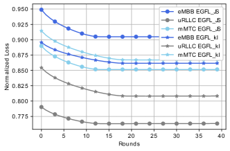
(a) Analysis of convergence with two approaches

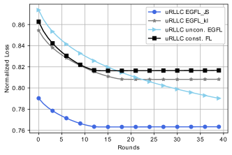
(b) Analysis of convergence with additional approaches for uRLLC slice

Figure 3: Analysis of FL training loss vs FL rounds of EGFL with lower bound of recall score, $\gamma=[0.82,0.85,0.84]$

VI Results

This section scrutinizes the proposed Closed loop EGFL framework.The dataset used in this study was generated through extensive simulations conducted within the framework described in the referenced paper [29]. The simulations involved generating diverse slice traffic profiles using heterogeneous Poisson distributions with time-varying intensities. These profiles were designed to accurately capture the distinctive behavior of each network slice. We use feature attributions generated by the XAI to build a fair sensitivity-aware, explanation-guided, constrained traffic drop prediction model. We also present the results corresponding to the fairness recall constraint and discuss its impact in detail. Moreover, we show FL convergence results and, finally, we analyze the comprehensiveness score of all slices to show the faithfulness of our proposed model. Notably, we invoke DeepExplain framework, which includes state-of-the-art gradient and perturbation-based attribution methods [30] to implement the Explainer for generating attribution scores of the input features. We integrate those scores with our proposed fair EGFL framework in a closed-loop iterative way.

VI-A Parameter Settings and Baseline

Three primary slices eMBB, uRLLC and mMTC are considered to analyze the proposed EGFL. Here, the datasets are collected from the BSs and the overall summary of those datasets are presented in Table II. We use vector $\alpha$ for the lower bound of recall score corresponding to the different slices. As a baseline, we adopt a vanilla FL [31] with post-hoc integrated gradient explanation, that is, a posterior explanation performed upon the end of the FL training.

Table III: Settings

Parameter	Description	Value
$N$	# Slices	$3$
$K$	# BSs	$50$
$D_{k,n}$	Local dataset size	$1500$ samples
$T$	# Max FL rounds	$40$
$U$	# Total users (All BSs)	$15000$
$L$	# Local epochs	$40$
$R_{\lambda}$	Lagrange multiplier radius	Constrained: $10^{-5}$
$\eta_{\lambda}$	Learning rate	$0.12$

VI-B Result Analysis

In this scenario, resources are allocated to slices according to their traffic patterns and radio conditions.In this section, we thoroughly compare our proposed EGFL-JS scheme to other compatible state-of-the-art baselines from various perspectives, such as convergence, fairness, and faithfulness analysis, to show its superior efficacy.

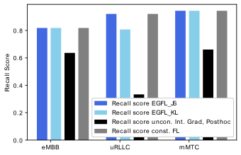
Figure 4: Analysis of recall score with lower bound $\gamma=[0.82,0.85,0.84]$

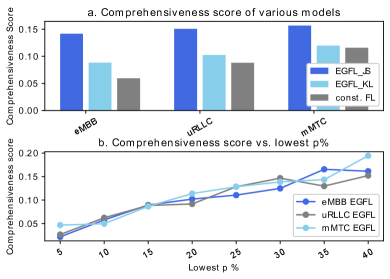
Figure 5: Analysis of comprehensiveness score with lower bound of recall score, $\gamma=[0.82,0.85,0.84]$

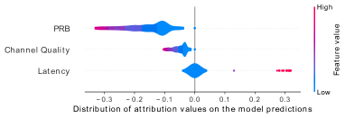
(a) Distribution plot for URLLC network slice

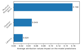
(b) Attribution-based feature impact on the model output for URLLC network slice

Figure 6: Root cause analysis of EGFL-JS predictions in a telecommunication network.

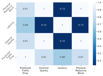
Figure 7: Correlation Heatmap for URLLC network slice

• Convergence: First, we have plotted FL normalized training loss vs. FL rounds of EGFL-JS, and shown the comparison with another compatible strategy termed EGFL-KL. The key distinction between the two techniques is the divergence measure used to guide their respective loss functions. The JSD guides the cross-entropy loss function in our proposed solution, whereas the EGFL-KL model uses the Kullback-Leibler Divergence (KL Divergence) to guide its loss function. It is known that JSD, a symmetrized variant of KL Divergence, is less sensitive to severe discrepancies across distributions, which may help speed up convergence. We visually depict both models’ convergence behavior across several slices in Fig. 3a. Notably, compared to the EGFL-KL model, our suggested model consistently shows a higher rate of convergence. This finding is consistent with what we predicted since JSD is naturally less susceptible to being impacted by severe distribution discrepancies, which results in a smoother optimization landscape and, as a result, faster convergence. Additionally, we broaden the scope of our research beyond the EGFL-KL model by including two additional methods: unconstrained EGFL (without recall constrained) and recall-constrained FL (without Jensen-Shannon Divergence). As depicted in Fig. 3b, we can conclude that the proposed constrained EGFL prediction model of the uRLLC slice has converged faster than the unconstrained EGFL. Moreover, compared to constrained FL, EGFL has given lower training losses. Overall, the empirical results shown in Fig. 3a and 3b support our proposed model’s improved convergence characteristics and demonstrate the benefits of including JSD in the loss function. These findings further strengthen the prospect of our concept as a highly efficient and successful solution in different real-world situations.

• Fairness Analysis: As illustrated in Fig. 4, the recall metric has been chosen to analyze our proposed model’s fairness. From that figure, we can observe that the recall score of the proposed EGFL-JS for all slices is closer to the target threshold $\lambda$ (i.e., around 0.80 $\%$), which would be an acceptable value for slices’ tenants. In summary, the recall scores of EGFL-JS, EGFL-KL and constrained FL for all slices are almost identical and higher than the unconstrained EGFL. In comparison, the training loss value of EGFL is lower than other approaches. The model with divergence included is better at generalizing to new, unseen data. However, having the same recall score indicates that the model’s ability to identify positive samples has not been affected by the inclusion of divergence, which is a favorable sign. This can be fruitful in cases where the model will be deployed in real-world applications, as it suggests that the model is more likely to perform well on new data that it has not seen during training. It gives us an approximate idea of our model’s reliability and trustworthiness.

• Faithfulness of Explanation: Comprehensiveness evaluates if all features needed to make a prediction are selected [7]. The model comprehensiveness is calculated as: Comprehensiveness = $\hat{y}_{k,n}^{(i)}-\tilde{p}_{k,n}^{(i)}$. Here, the higher score implies that the explanation provided is complete, comprehensive, and so helpful to the user. In Fig. 5 we have plotted the comprehensiveness score of all the slices, where we notice that the proposed EGFL has a higher score than the EGFL-KL and baseline one. Moreover, in Fig. 5b, we monitor the effect of the changing value of the p$\%$ features removal on the comprehensiveness score, considering the proposed model for all slices. Specifically, during the calculation of comprehensiveness score based on the removal of $p\%$ of features with lowest attributions, we have created a new masked input, denoted as $\tilde{\mathbf{x}}_{k,n}^{(i)}$ for each p$\%$ value and also have generated the corresponding masked predictions, $\tilde{p}_{k,n}^{(i)}$. Here, the score increases versus the lowest $p\%$, which means that the masked features are decisive and the corresponding explanation in terms of attribution is comprehensive.

• Root cause analysis in wireless networks and Interpretation: Feature attributions generated by XAI methods reflect the contribution of the input features to the output prediction. From a telecommunication point of view, this can be leveraged to perform root cause analysis of different network anomalies and KPIs degradation. In this respect, we investigate the factors that impact slice-level packet drop by plotting, for instance, the distribution of the URLLC slice feature attributions in Fig. 6a and their average in Fig. 6b. The first subfigure demonstrates that EGFL traffic drop predictions are negatively influenced by PRB and the channel quality, since the attributions are distributed and concentrated towards negative values, implying that higher values of these features reduce the likelihood of traffic drops. It is noted that PRB has a slightly higher impact compared to channel quality. In this regard, Fig. 6b further supports these observations by confirming that in average PRB has the most influence on the model’s output, reaffirming the importance of PRB allocation in reducing traffic drops. This observation aligns with the notion that higher PRB allocation implies dedicating more resources to the URLLC slice, which in turn relaxes the transmission queues and reduces the packet drop. Lastly, the distribution and average plots reveal that latency has a narrower and more focused distribution near zero. This suggests that latency may have lesser significance in predicting traffic drops compared to other features. Furthermore, the correlation heatmap of Fig. 7 indicates the strength and direction of the linear relationship between the predicted traffic drops and each input feature, namely PRB, channel quality, and latency with a correlation of 81 $\%$, 81 $\%$ and 69 $\%$ respectively., which corroborates the previous analysis. Note that to plot correlation matrix heatmap, we consider one matrix, $\mathbf{R}_{k,n}$ = [$\mathbf{a}_{k,n},\hat{\mathbf{y}}_{k,n}$], where, $\mathbf{a}_{k,n}$ denotes the attribution score of features with dimensions $D_{k,n}\times Q$ and $\hat{\mathbf{y}}_{k,n}$ is the predicted output variable with dimensions $D_{k,n}\times 1$. A correlation of 81 $\%$ between the predicted traffic drops and PRB as well as channel quality suggests a strong positive relationship. This means that higher values of PRB and channel quality are associated with a higher likelihood of lower traffic drops in the URLLC slice. On the other hand, the correlation coefficient of 69 % between the predicted traffic drops and latency indicates a moderate positive relationship. This means that higher values of latency are generally associated with a higher likelihood of traffic drops in the URLLC slice. Based on these observations, it can be inferred that when dealing with real-time traffic in the telecom industry, maintaining an appropriate allocation of PRB and monitoring channel quality in the network slice becomes crucial for ensuring better services to users.

VII Conclusion

In this paper, we have proposed a novel fair explanation guided federated learning (EFGL) approach to fulfill transparent and trustworthy zero-touch service management of 6G network slices at RAN in a non-IID setup. We have proposed a modified objective function where we consider Jenson-Shannon divergence along with the cross-entropy loss and a fairness metric, namely the recall, as a constraint. The underlying optimization task has been solved using a proxy-Lagrangian two-player game strategy. The simulated results have validated that the proposed scheme can give us a new direction for implementing trustworthy and fair AI-based predictions.

VIII Acknowledgment

This work has been supported in part by the project SEMANTIC (861165). It has also been supported in part by the MINECO (Spain) and the EU NextGenerationEU/PRTR (Call UNICO I+D 5G 2021, ref. number TSI-063000-2021-10)

References

- [1] C. Benzaid and T. Taleb, “AI-driven zero touch network and service management in 5G and beyond: Challenges and research directions,” IEEE Network, vol. 34, no. 2, pp. 186–194, 2020.
- [2] S. Jha and S. R. and others, “Attribution-based confidence metric for deep neural networks,” in Neural Information Processing Systems, 2019.
- [3] M. Naylor, C. French et al., “Quantifying explainability in NLP and analyzing algorithms for performance-explainability tradeoff,” in Proceedings of the Thirty-eighth International Conference on Machine Learning, 2021.
- [4] S. Roy, H. Chergui, and C. Verikoukis, “TEFL: Turbo Explainable Federated Learning for 6G Trustworthy Zero-Touch Network Slicing,” 2022. [Online]. Available: https://arxiv.org/abs/2210.10147
- [5] A. A. Ismail, H. Corrada Bravo, and S. Feizi, “Improving deep learning interpretability by saliency guided training,” Advances in Neural Information Processing Systems, vol. 34, pp. 26 726–26 739, 2021.
- [6] K. Li, Z. Wu, and a. Peng, “Tell me where to look: Guided attention inference network,” in Proceedings of the IEEE conference on computer vision and pattern recognition, 2018, pp. 9215–9223.
- [7] Y. Gao, S. Gu, and a. Junji Jiang, “Going beyond XAI: A systematic survey for explanation-guided learning,” ArXiv, vol. abs/2212.03954, 2022.
- [8] B. Brik and A. Ksentini, “On predicting service-oriented network slices performances in 5G: A federated learning approach,” in 45th IEEE Conference on Local Computer Networks, LCN 2020, Sydney, Australia, November 16-19, 2020, H. P. Tan, L. Khoukhi, and S. Oteafy, Eds. IEEE, 2020, pp. 164–171. [Online]. Available: https://doi.org/10.1109/LCN48667.2020.9314849
- [9] C. Li, W. Guo, and a. Sun, “Trustworthy deep learning in 6G-enabled mass autonomy: From concept to quality-of-trust key performance indicators,” IEEE Vehicular Technology Magazine, vol. 15, no. 4, pp. 112–121, 2020.
- [10] A. Terra and a. Inam, “Explainability methods for identifying root-cause of SLA violation prediction in 5G network,” in GLOBECOM 2020 - 2020 IEEE Global Communications Conference, 2020, pp. 1–7.
- [11] S. Wang, M. Qureshi, and a. Luis Miralles-Pechua’an, “Explainable AI for B5G/6G: Technical aspects, use cases, and research challenges,” ArXiv, vol. abs/2112.04698, 2021.
- [12] M. Munir, K. T. Kim, and a. Adhikary, “Neuro-symbolic explainable artificial intelligence twin for zero-touch IoE in wireless network,” arXiv preprint arXiv:2210.06649, 2022.
- [13] A. Renda and o. Ducange, Pietro and, “Federated learning of explainable AI models in 6G systems: Towards secure and automated vehicle networking,” Information, vol. 13, no. 8, 2022. [Online]. Available: https://www.mdpi.com/2078-2489/13/8/395
- [14] T. Popordanoska, M. Kumar, and S. Teso, “Machine guides, human supervises: Interactive learning with global explanations,” ArXiv, vol. abs/2009.09723, 2020.
- [15] A. S. Ross and M. C. H. and others, “Right for the right reasons: Training differentiable models by constraining their explanations,” in International Joint Conference on Artificial Intelligence, 2017.
- [16] Y. Gao and T. a. Sun, “Gnes: Learning to explain graph neural networks,” in 2021 IEEE International Conference on Data Mining (ICDM), 2021, pp. 131–140.
- [17] J. Sun and S. L. and others, “Explanation-guided training for cross-domain few-shot classification,” 2020 25th International Conference on Pattern Recognition (ICPR), pp. 7609–7616, 2020.
- [18] W. Wu, C. Zhou, and a. Li, “AI-native network slicing for 6G networks,” IEEE Wireless Communications, vol. 29, no. 1, pp. 96–103, 2022.
- [19] H. Chergui and L. a. Blanco, “Statistical federated learning for beyond 5G SLA-constrained RAN slicing,” IEEE Transactions on Wireless Communications, vol. 21, no. 3, pp. 2066–2076, 2022.
- [20] A. Cotter, H. Jiang, and K. Sridharan, “Two-player games for efficient non-convex constrained optimization,” CoRR, vol. abs/1804.06500, 2018. [Online]. Available: http://arxiv.org/abs/1804.06500
- [21] M. Glockner et al., “Why do you think that? exploring faithful sentence-level rationales without supervision,” in Findings of the Association for Computational Linguistics: EMNLP 2020. Online: Association for Computational Linguistics, Nov. 2020, pp. 1080–1095. [Online]. Available: https://aclanthology.org/2020.findings-emnlp.97
- [22] Y. K. Tun and N. H. T. and others, “Wireless network slicing: Generalized kelly mechanism-based resource allocation,” IEEE Journal on Selected Areas in Communications, vol. 37, pp. 1794–1807, 2019.
- [23] M. Sundararajan, A. Taly, and Q. Yan, “Axiomatic attribution for deep networks,” in Proceedings of the 34th International Conference on Machine Learning - Volume 70, ser. ICML’17. JMLR.org, 2017, pp. 3319–3328.
- [24] A. Cotter and a. Maya R. Gupta, “Training well-generalizing classifiers for fairness metrics and other data-dependent constraints,” in ICML, 2019.
- [25] G. J. Gordon, A. Greenwald, and C. Marks, “No-regret learning in convex games,” in Proceedings of the 25th International Conference on Machine Learning, ser. ICML ’08. New York, NY, USA: Association for Computing Machinery, 2008, pp. 360–367. [Online]. Available: https://doi.org/10.1145/1390156.1390202
- [26] T. Yamano, “Some bounds for skewed -jensen-shannon divergence,” Results in Applied Mathematics, vol. 3, p. 100064, 2019. [Online]. Available: https://www.sciencedirect.com/science/article/pii/S2590037419300640
- [27] J. Lin, “Divergence measures based on the shannon entropy,” IEEE Transactions on Information Theory, vol. 37, no. 1, pp. 145–151, 1991.
- [28] W. Hoeffding, “Probability inequalities for sums of bounded random variables,” Journal of the American Statistical Association, vol. 58, no. 301, pp. 13–30, 1963. [Online]. Available: http://www.jstor.org/stable/2282952
- [29] F. Rezazadeh and L. a. Zanzi, “On the specialization of FDRL agents for scalable and distributed 6G ran slicing orchestration,” IEEE Transactions on Vehicular Technology, vol. 72, no. 3, pp. 3473–3487, 2023.
- [30] [Online]. Available: https://github.com/marcoancona/DeepExplain
- [31] H. B. McMahan and a. Eider Moore, “Communication-efficient learning of deep networks from decentralized data,” in International Conference on Artificial Intelligence and Statistics, 2016.