Forecasting the steam mass flow in a powerplant using the parallel hybrid network

Abstract

Efficient and sustainable power generation is a crucial concern in the energy sector. In particular, thermal power plants grapple with accurately predicting steam mass flow, which is crucial for operational efficiency and cost reduction. In this study, we use a parallel hybrid neural network architecture that combines a parametrized quantum circuit and a conventional feed-forward neural network specifically designed for time-series prediction in industrial settings to enhance predictions of steam mass flow 15 minutes into the future. Our results show that the parallel hybrid model outperforms standalone classical and quantum models, achieving more than 5.7 and 4.9 times lower mean squared error (MSE) loss on the test set after training compared to pure classical and pure quantum networks, respectively. Furthermore, the hybrid model demonstrates smaller relative errors between the ground truth and the model predictions on the test set, up to 2 times better than the pure classical model. These findings contribute to the broader scientific understanding of how integrating quantum and classical machine learning techniques can be applied to real-world challenges faced by the energy sector, ultimately leading to optimized power plant operations.

I Introduction

Quantum-enhanced machine learning (or quantum machine learning, QML) has emerged as a rapidly growing field, combining quantum computing with machine learning to develop new models with the potential to revolutionize data analysis dunjko2018machine ; Melnikov_2023 . A popular approach to QML uses trainable quantum circuits as machine learning models similar to widely known classical neural networks. These circuits consist of encoding and variational unitary gates. The former maps classical data into quantum states, while the latter are parameterized gates trained using classical optimizers to minimize a cost function. The output of the circuit is obtained by measuring an observable on the final state, which produces a vector of real numbers representing the model’s prediction. This approach is known in the literature as parametrised quantum circuits (PQCs) benedettipaper ; jerbi2021parametrized , quantum neural networks (QNNs) farhi2018classification ; bp ; kordzanganeh2023exponentially , variational quantum circuits skolik2022quantum ; McClean_2016 ; romero2019variational or quantum circuit learning Mitarai_2018 . These models are a promising direction for the future of ML.

It has been demonstrated on toy datasets that QML models need fewer steps to converge smaller error aselpaper2 ; amirapaper and have better generalisation ability from fewer data points aselpaper2 ; Generalization_QML compared to their classical counterparts. However, today, the quantum computing infrastructure cannot yet create competitive quantum models to tackle real-world, ill-structured data science problems schuld-advantage . This is only exacerbated by the barren plateau problem, discovered in bp , suggesting that large QML models are challenging to train high qubit count. Since NISQ devices limit the freedom in the machine learning model choice, research is instead focused on the hybrid quantum neural networks (HQNN) paradigm – a combination of classical and quantum models aselpaper2 ; aselpaper1 . It was shown aselpaper1 ; sagingalieva2023hybrid ; rainjonneau2023quantum ; senokosov2023quantum ; sedykh2023quantum that such models can outperform classical counterparts, making this concept attractive for further research.

Classical machine learning techniques have been widely used in the energy sector for various applications, including time series prediction. One common use case is forecasting energy demand or generation to enable effective planning and operation of energy systems cassical_ml_energy_1 ; cassical_ml_energy_2 ; cassical_ml_energy_3 . However, in this work, we successfully attempted to solve such kind of real-world problem using HQNN. In partnership with Uniper, we predicted the average steam mass flow exiting a thermal power plant 15 minutes ahead. This was done by creating a novel HQNN architecture that, unlike most previous works mari2020transfer ; zhao2019qdnn ; dou2021unsupervised ; sebastianelli2021circuit ; pramanik2021quantum ; aselpaper2 ; aselpaper1 ; sagingalieva2023hybrid ; rainjonneau2023quantum where the quantum and classical networks were arranged sequentially to feed information to each other, were placed parallelly. This creates a complementary network where each element, quantum and classical, play its role.

The structure of the paper is as follows. Section II provides context for the power plant, specifies the abstractions required to convert this into a data science problem and describes the dataset. Section III gives the pre-processing steps, baseline classical and hybrid architectures. Then we present the details of our model training and performance results, comparing our hybrid model with the fully quantum and classical counterparts in Section IV. Our work concludes with discussing our findings in Section V. Additionally, we offer an analysis of our quantum circuit in the Appendix.

II Problem statement and context

II.1 Uniper Operaite

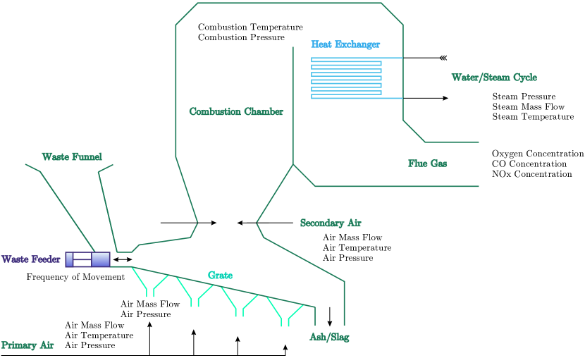
Figure 1: The structure of a typical grate-fired boiler in a waste-to-energy power plant. The waste is dropped into the funnel above the waste feed by a crane, typically a few tons at once. Then, the hydraulic waste feed, which moves back and forth, pushes the waste onto the grate. The grate is divided into a few subsequent zones, which can be moved independently while combustion air enters the chamber from the bottom. The main combustion typically occurs in the second and third zone on the grate, which are in the middle of the grate. The resulting flue gases stream upwards and then along the predefined way until the chimney is reached, where flue gases exit into the atmosphere. On the way, the flue gases pass by the heat exchange mechanisms (pipes), transferring heat energy to the water steam cycle. Eventually, superheated steam is fed into a steam turbine to generate electricity. Measurements are placed all over the boiler and produce time series data around the clock. This data is used to monitor and control the process but can likewise be used to build machine learning models, as we do in this paper.

A thermal power plant operates by converting heat energy into electricity through a series of processes involving fuel combustion, heat exchange, and steam generation. In waste-to-energy and biomass-to-energy power plants, solid waste or biomass is used as fuel. The combustion process generates hot flue gases, which transfer heat to water, turning it into steam. The superheated steam drives a turbine connected to a generator, which produces electricity. Throughout the power plant, numerous sensors measure parameters such as steam mass flow, air flows, waste feed, temperatures, and chemical concentrations in the flue gas. This data is crucial for monitoring and controlling the plant’s operation and developing machine learning models for forecasting and optimization purposes.

Predicting steam mass flow in a thermal power plant is essential for maintaining operational stability, optimizing energy output, controlling emissions, planning maintenance activities, and reducing costs. Accurate forecasts of steam mass flow enable operators to make informed decisions about adjusting various parameters, such as fuel input and air supply, to ensure smooth and efficient operation. Furthermore, predicting steam mass flow can help in controlling emissions generated by the power plant, minimizing the production of pollutants that negatively impact the environment and public health.

In the Operaite team at Uniper, combustion processes are optimized using conventional, fully-connected feed-forward neural networks. In waste-to-energy and biomass-to-energy power plants, combustion processes are highly dynamic due to volatile fuel quality resulting, e.g. from varying geometric or chemical properties of the typically solid fuel components. This corresponds to continuous stimulation of the combustion process and constantly changes the equilibrium of the combustion process, which is given by a certain ratio between fuel infeed and airflow. Thus, continuous control (of, e.g., the airflow) is needed to maintain a steady and stable operation, which is usually achieved by using CCS (combustion control systems). Various CCSs exist, ranging from simple conventional systems built from combinations of PID (proportional-integral-derivative) controllers over fuzzy or rule-based systems to model predictive control. Most power plants rely on PID controllers, and only a few employ more advanced process control techniques, mainly because implementing them takes a lot of time and is related to high costs. Typical optimization goals could be to increase or smooth the energy output in terms of steam mass flow or electricity generation or to reduce emissions in terms of CO or NOx concentrations in the flue gas. There are two ways to achieve these operational goals, which are (i) using a controlling neural network that directly interacts with control levers and (ii) using a neural network that provides forecasts and serves as an assistant system to help humans manipulate the process proactively. This paper concentrates on improving (ii) by employing hybrid quantum neural network forecasts.

II.2 Forecasting problem

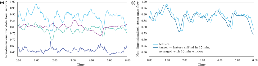
Figure 2: Feature and target data used for time series prediction. (a) Features consist of $192$ time series, including steam mass flow, with the first four-time series displayed for clarity over $6$ hours. (b) Target data shows steam mass flow values shifted $15$ minutes into the future and averaged over a $10$-minute interval, displayed only for the first sensor for simplicity. Note that the shifted and averaged signal will be used by human operators as an early indicator for problematic process situations. This indication will help them to take proactive actions.

In this section, we present the problem statement and discuss the dataset from the power plant for forecasting problems. The objective is to develop a model that can predict the steam mass flow for two sensors $15$ minutes into the future based on the current values of all the power plant parameters, including air flows, waste feed, temperatures, chemical concentrations in the flue gas, and steam mass flow, among others. Thus, we solve a multivariate regression problem in continuous space.

The prediction timeframe is determined by the characteristic timescales of the combustion process, which are depicted in Fig. 1. The combustion process entails several stages, including waste feeding, transport across the grate, flue gas stream, and heat exchange. The airflow needs to be changed continuously in response to fuel quality changes. Assuming a constant fuel quality, the system requires $5$ to $15$ minutes to return to equilibrium. Consequently, we deemed it appropriate to consider a prediction horizon of $15$ minutes for this task. Thus, the forecasted timeframe should be sufficient to take appropriate action early enough.

Feature and target data used in our study are represented in Fig. 2. The dataset consists of $192$ time series, which are our features, each representing measurements of power plant parameters captured by various sensors throughout the facility, also including numerical derivatives and moving averages for each sensor. The targets we aim to predict are represented by two time series. Specifically, each target variable corresponds to the steam mass flow value for a given sensor that has been shifted $15$ minutes into the future and averaged over a $10$-minute window. This averaging process is intended to create a more uniform steam mass flow signal and reduce fluctuations. Our training dataset consists of $6,500$ timestamps, which only represent $1\%$ of the original dataset used to train the classical model currently in production. We chose to reduce the dataset due to the time-consuming nature of training a quantum neural network using existing simulatorskordzanganeh2023benchmarking . Nevertheless, it is worth noting that quantum neural networks are better at generalising from fewer data points Generalization_QML . Therefore, such a simplification can be considered justified.

III Machine learning models

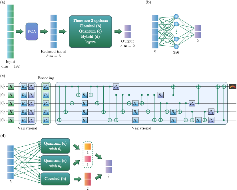
Figure 3: (a) Problem definition and general pipeline of solution. The task is to predict steam mass flow for two sensors at time $t+15$ min, given values of multiple time series (192) from different sensors at time $t$. The input vector $\mathbf{x}$ is pre-processed with PCA to reduce the feature space from $192$ to $5$. Then, an appropriate machine learning algorithm (classical, quantum, or hybrid) is applied to reduced input to predict the output, which is a $2$-dimensional vector corresponding to the target value for each of the two sensors. (b) Classical neural network architecture. The architecture consists of $5$ input neurons, $256$ hidden neurons, and $2$ output neurons. (c) Parameterized quantum circuit (PQC). The quantum circuit includes $5$ qubits and a set of encoding and variational gates. The first qubit is measured in the $Z$-basis to yield a real-valued output. (d) shows the parallel hybrid network architecture. The architecture consists of a classical neural network and two identical PQCs that operate independently. Each of them takes a $5$-dimensional reduced input. The classical and quantum predictions are added to the corresponding components, resulting in the final output.

III.1 Pre-processing

An effective pre-processing of data is crucial for any machine learning pipeline, especially when dealing with quantum neural networks. The scarcity of qubits on physical quantum computers and the high computational cost of PQCs simulations are significant challenges in this field kordzanganeh2023benchmarking ; tang2022cutting . However, even small quantum networks combined with classical ones can still achieve supremacy in some cases. It is important to transform the data into a space with dimensions suitable for quantum processing to overcome this challenge. In our approach, we use principal component analysis (PCA), a powerful data analysis technique that reduces the dimensions of the original dataset Hill2016PythonML . By projecting the data onto the five main components, we reduce the input vector dimension from $192$ to $5$ while retaining more than $60\%$ of the original data’s contribution share as illustrated in Fig. 4(a). We then standardize and normalize the data, which typically has varying scales. These pre-processing steps prepare the data for processing with PQC, for which appropriate architectures will be introduced below.

III.2 Classical baseline architecture

A classical baseline architecture was utilised to enable future comparisons with hybrid solutions. This architecture is a fully connected neural network with one hidden layer, consisting of $5$ input neurons, $256$ hidden neurons, and $2$ output neurons, as illustrated in Fig. 3(b). It is important to note that the design of the baseline model was inspired by an existing model currently in production, which addresses a similar problem of multivariate regression. However, the difference lies in the number of targets, as the production model predicts more parameters for various sensors, while our model only predicts steam mass flow for two sensors. The architecture of the production model is also a conventional feed-forward neural network with one hidden layer.

Although the forecasting problem can be effectively solved using recurrent neural networks, such as LSTM models RNN_paper ; LSTM_paper or more advanced Transformer-based architectures vaswani2017attention , conventional feed-forward neural networks with a more straightforward structure are generally easier to train and faster to process. Conventional neural networks have the advantage that the forward pass, which is necessary for the production environment, can be efficiently implemented on a controller compatible with the distributed control system in a power plant. In addition, conventional feed-forward neural networks provide better explainability compared to more advanced network topologies. For this reason, we used a conventional feed-forward neural network for our baseline architecture in this research.

III.3 Hybrid quantum-classical architecture

A good understanding of the data structure is crucial in building an effective architecture for problem-solving. In our case, our goal is to predict the values of a time series at a given time. By analyzing Fig. 2, we can observe that the prediction follows a sinusoidal pattern with some irregularities. It is known that a classical neural network with one hidden layer is an asymptotically universal approximator. This was also shown for parameterised quantum circuits (PQC) - quantum neural networks capable of universal approximation schuld_fourier . However, PQCs achieve this by fitting a truncated Fourier series over the samples. With this in mind, we use the parallel hybrid network (PHN) configuration introduced in kordzanganeh2023parallel , which differs from the previous sequential quantum-classical hybrid models mari2020transfer ; zhao2019qdnn ; dou2021unsupervised ; sebastianelli2021circuit ; pramanik2021quantum ; aselpaper2 ; aselpaper1 ; sagingalieva2023hybrid ; rainjonneau2023quantum . Here, the quantum and classical parts process the data independently and simultaneously without interfering with each other. The quantum circuit approximates the sinusoidal part, while the classical network fits the protruding sections. Finally, the predictions from both parts are combined to obtain the final prediction. This approach lets the classical model only adjust its weights and does not interfere with the quantum circuit during the training procedure.

The proposed architecture comprises two identical parameterized quantum ansatz circuits, which will be introduced below, and a classical fully-connected neural network, discussed in Section III.2 and illustrated in Figure 3(b). The complete PHN architecture is depicted in Figure 3(d), with the same feature vector as input to both the classical and quantum circuits. Before this, the input feature vector undergoes a PCA procedure to reduce its dimensions from 192 to 5.

The quantum layer (PQC) depicted in Figure 3(c) consists of five qubits. The layer begins with applying a Hadamard transform to each qubit, followed by a sequence of variational gates consisting of rotations along the $z$ and $x$ axes for each qubit. The reduced input data (with a dimensionality of 5) is then embedded into the rotation angles along the $z$-axis. Subsequently, another variational block is applied, consisting of a sequence of $R_{ZZ}$ gates that alternate periodically with rotations along the $x$-axis and conventional CNOT gates. The complete gate sequence can be found in Figure 3(c). Finally, the local expectation value of the Z operator is measured for the first qubit, producing a classical output suitable for additional post-processing. In the Appendix, we analyze a simplified version of this quantum circuit using three approaches to assess its efficiency, trainability, and expressivity.

The predictions of the classical network and the quantum circuits are combined to generate the final prediction. Specifically, the output of the first quantum circuit is added to the first component of the classical network’s prediction vector. In contrast, the output of the second quantum circuit is added to the second component of the vector. This results in the final classical-quantum output, which has the potential to enhance accuracy and efficiency for time series prediction.

IV Training and results

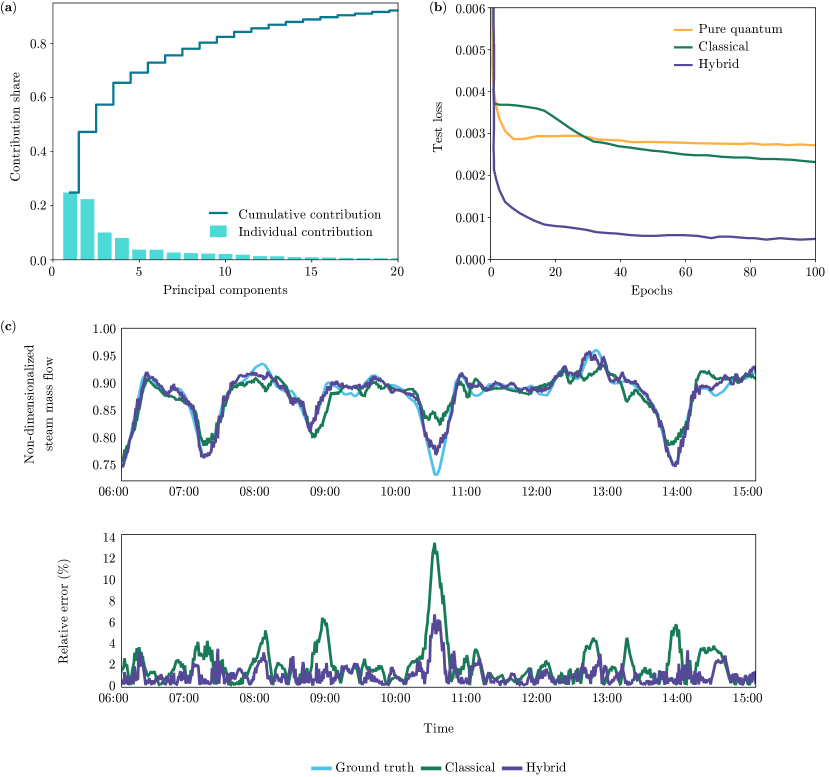
Figure 4: (a) The results of the principal component analysis (PCA). We can see that the first five principal components cover a significant majority of the contribution share. (b) Loss performance comparison between the hybrid, pure classical, and pure quantum models. We see that while they each perform sub-optimally separately, classical and quantum networks can form a hybrid network that outperforms both by a significant margin. (c) The fit of the classical and hybrid circuit to the time series in the test region. The top graph shows the classical and hybrid predictions on unseen data. In contrast, the bottom graph shows its residuals – relative errors between ground truth and the model prediction at each point.

When using this architecture, one must take extra caution when tuning the hyper-parameters. This arises due to the separability of the three parallelized architectures. It is important to make sure none of the 3 fully dominates the training, resulting in a model stuck in a local minimum. For this reason, we make sure that the quantum network has the chance to train first to create a sinusoidal landscape, and then the classical network begins to contribute. We do this by reducing the learning rate of the classical parameters compared with the quantum ones. This ensures that the quantum networks can train and fit a sinusoidal function before the classical make any real contribution. At some point in the training, the quantum network has achieved a minimum, and its gradient values are so small that the classical network begins its meaningful training stage.

All machine learning experiments were conducted on the QMware cloud platform qmw_qmw_2022 . PyTorch library pas_pyt_2019 was used to implement the classical part, while the quantum one was implemented using the PennyLane framework ber_pen_2022 . We used the lightning.qubit device, which implements a high-performance C++ backend. The standard backpropagation algorithm was applied to the classical part of our hybrid quantum neural network to calculate the loss function’s gradients for each parameter. In contrast, the adjoint method was employed for the quantum part.

In Fig. 4(b), the loss performance is presented for the hybrid architecture compared to the purely classical and purely quantum networks. The pure classical network exclusively employs the classical neural network, whereas the pure quantum network utilizes only the two quantum models in the absence of classical components. It is evident from the results that the hybrid architecture outperforms the pure classical and pure quantum counterparts by a significant margin. Specifically, after 100 epochs of training, the mean squared error (MSE) loss for the hybrid architecture is more than 5.7 and 4.9 times lower than that of the purely classical and purely quantum networks. Fig. 4(c) shows the fit of the classical and hybrid circuits to the time-series data in the test region. The top graph displays the classical and hybrid predictions on unseen data. In contrast, the bottom graph depicts their residuals, representing the relative errors between the ground truth and the model predictions at each point. Overall, the hybrid model predictions are much closer to the ground truth with a smaller relative error, up to 2 times lower than the classical approach. Therefore, a PHN-based approach is the most efficient strategy in this case.

V discussion

This study has highlighted the potential of quantum machine learning for time series prediction in the energy sector through a novel parallel hybrid architecture. We have demonstrated superior performance to traditional classical and quantum architectures by combining independent classical and quantum neural networks. Our approach enables the classical and quantum networks to operate independently during the training, preventing interference between the two.

Our results reveal that the parallel hybrid model outperforms pure classical and pure quantum networks, exhibiting more than 5.7 and 4.9 times lower MSE loss on the test set after training. Furthermore, the hybrid model demonstrates more minor relative errors between the ground truth and the model predictions on the test set, up to 2 times better than the pure classical model.

These findings suggest that quantum machine learning can be valuable for solving real-world problems in the energy sector and beyond. Future research could explore applying the parallel hybrid quantum neural network approach to other machine learning problems while also increasing the complexity and performance of the model.

APPENDIX

Quantum Circuit Analysis

In this section, we thoroughly examine a parameterized quantum circuit (PQC) that is represented in Fig. 5(a). This PQC is a 2-qubit toy version introduced in Section III.3, inheriting its fundamental properties and concepts. Our analysis focuses on three different approaches: the ZX-calculus [40] to examine circuit-reducibility, the Fisher information [13] to evaluate the trainable parameters and the circuit expressiveness, and the Fourier accessibility [35] to investigate the encoding.

.1 ZX-calculus

The ZX-calculus is a graphical language initially based on Category Theory that can simplify a quantum circuit to a simpler, equivalent one [40]. It involves transforming the circuit into a ZX graph and applying the ZX-calculus rules introduced in Ref. [41] to reduce the graph to a more fundamental version. After that, the obtained version is mapped again to the quantum circuit. This process results in a new, streamlined circuit that achieves the maximum potential of trainable layers while avoiding fully redundant parameters. If a circuit cannot be further reduced, it is called ZX-irreducible.

In this study, we present a novel quantum circuit that generates a non-commuting graph which cannot be simplified using ZX-calculus rules. This is illustrated in Fig. 5(b), where adjacent dots are colored differently. Notably, the X-spiders (red dots) appear only at the first wire’s end, and the measurement is performed in the Z-basis (green family). Consequently, no pairs of dots can commute with each other, and none of them can fuse. This implies that our circuit has no redundant parameters.

Remarkably, our circuit is designed only to measure the first qubit. At the same time, the encoding and variational parameters of the second qubit (in the original circuit with the other four qubits) heavily influence the measurement outcome of the first qubit. This is achieved using the $R_{ZZ}$ gate, namely parameter $\alpha_{5}$ introduces pairwise correlations between the $x_{1}$ and $x_{2}$ features (in the original circuit, such correlations create between any pair of qubits). As a result, we obtain a highly complex approximator that depends on the features in a non-trivial manner. The subsequent sections present a detailed analysis of such a quantum approximator’s qualities.

.2 Fisher information

Any neural network, classical or quantum, can be considered a statistical model. The Fisher information estimates the knowledge gained by a particular parameterization of such a statistical model. In supervised machine learning, we are given a set of data pairs $(\mathbf{x},y)$ from a training subset and a parameterized model $h_{\boldsymbol{\theta}}(\mathbf{x})$ that maps input data $\mathbf{x}$ to output $y$. The parameterized models family can be fully described by the joint probability of features and targets: $\mathcal{F}:=\{P(\mathbf{x},\mathbf{y}|\boldsymbol{\theta}):\boldsymbol{\theta}\in\boldsymbol{\Theta}\}$ and during the training procedure, we want to maximize likelihood to determine the parameters $\boldsymbol{\hat{\theta}}\in\boldsymbol{\Theta}$ for which the observed data have the highest joint probability. We can think of $\mathcal{F}$ as some Riemannian manifold, and the Fisher information matrix can be naturally defined as a metric over this manifold [42, 13]:

$$F(\boldsymbol{\theta})=\mathbb{E}_{\{(\mathbf{x},\mathbf{y})\sim p\}}[\boldsymbol{\nabla}_{\boldsymbol{\theta}}\log p(\mathbf{x},\mathbf{y}|\boldsymbol{\theta})\cdot\boldsymbol{\nabla}_{\boldsymbol{\theta}}\log p(\mathbf{x},\mathbf{y}|\boldsymbol{\theta})^{T}]$$ (1)

According to the findings presented in Ref. [13], when the number of qubits in a model increases, a Fisher information spectrum with a higher concentration of eigenvalues approaching zero indicates that the model potentially suffers from a barren plateau. On the other hand, if the Fisher information spectrum is not concentrated around zero, it is less likely for the model to experience a barren plateau.

Using the Fisher information matrix, we can also describe model capacity: quantifying the class of functions, a model can fit, in other words, a measure of the model’s complexity. For this purpose, the notion of effective dimension, firstly introduced in Ref. [43] and modified in Ref. [13], can be used:

$$d_{\gamma,n}(\mathcal{M}_{\Theta}):=2\frac{\text{log}\left(\frac{1}{V_{\Theta}}\int_{\Theta}\sqrt{\text{det}\left(id_{d}+\frac{\gamma n}{2\pi\text{log}n}\hat{F}(\boldsymbol{\theta})\right)}d\boldsymbol{\theta}\right)}{\text{log}\left(\frac{\gamma n}{2\pi\text{log}n}\right)},$$ (2)

where $V_{\Theta}:=\int_{\Theta}d\theta$ is the volume of the parameter space, $\gamma$ is some constant factor [13], and $\hat{F}(\boldsymbol{\theta})$ is the normalised Fisher matrix defined as

$$\hat{F}_{ij}(\boldsymbol{\theta}):=d\frac{V_{\Theta}}{\int_{\Theta}\operatorname{Tr}(F(\boldsymbol{\theta}))d\boldsymbol{\theta}}F_{ij}(\boldsymbol{\theta}).$$ (3)

We calculate the Fisher information for three specific toy circuit configurations: with $N=1$ last trainable layer repetition - contains $7$ trainable parameters, when $N=2$ and $N=3$ repetitions that consist of $10$ and $13$ trainable parameters accordingly. For a finite number of data, taking into account definition (1), the Fisher information estimate with some simplifications can be rewritten as follows:

$$F(\boldsymbol{\theta})=\sum_{(\mathbf{x},\mathbf{y})\in X\times Y}\frac{\boldsymbol{\nabla}_{\boldsymbol{\theta}}P(\mathbf{x},\mathbf{y}|\boldsymbol{\theta})\cdot\boldsymbol{\nabla}_{\boldsymbol{\theta}}P(\mathbf{x},\mathbf{y}|\boldsymbol{\theta})^{T}}{P(\mathbf{x},\mathbf{y}|\boldsymbol{\theta})},$$ (4)

where the joint probability for QNN can be defined as the overlap between model output and these states:

$$P(\mathbf{x},\mathbf{y}|\boldsymbol{\theta})=\operatorname{Tr}(\rho(\boldsymbol{\theta},\mathbf{x})\cdot\mathbf{y}\mathbf{y}^{\dagger}).$$ (5)

Following Ref. [13], we used $1000$ features samples, each of them comes from Gaussian distribution $\mathbf{x_{i}}\sim\mathcal{N}(\mu=0,\sigma^{2}=1)$, and target as specific resultant state $\mathbf{y}\in Y=\{\left|00\right\rangle,\left|01\right\rangle,\left|10\right\rangle,\left|11\right\rangle\}$ which are all possible basis states since we deal with the 2-qubit circuit. The Fisher information matrix is calculated with $100$ uniform weights realization $\theta\in[0,2\pi)$.

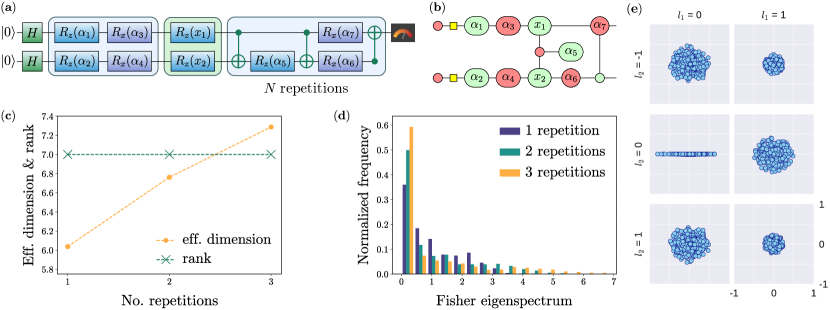
Figure 5: (a) Toy version of PQC used as a part of parallel HQNN in our study. (b) The ZX-calculus graph representation for PQC. No fundamental simplification; measurement is done in Z-basis, which ensures non-commutativity with previous gates. (c) Effective dimension and rank of the average Fisher information matrix for different repetitions $N={1,2,3}$ with $7,10$ and $13$ trainable parameters correspondingly. Not maximal rank for networks with $N={2,3}$ indicates the presence of zero gradient parameters. (d) Fisher information matrix normalized eigenspectrum frequency. The degeneracy about zero means lower trainability. (e) The Fourier accessibility. The set characterizes the possible values of the particular Fourier coefficient.

Figure 5(c) shows how the average Fisher information matrix’s effective dimension and rank depend on the network’s trainable layers. As expected, the effective dimension increases with the number of trainable parameters, indicating an increase in expressivity. However, trainability is also an important factor. The spectrum of the Fisher information matrix reflects the square of the gradients [13], and a network with high trainability will have fewer eigenvalues close to zero.

Our experiments found that the Fisher information matrix rank remained constant at $7$ for all three configurations, indicating the presence of zero gradients for some network parameters with $10$ and $13$ trainable parameters. This is further illustrated in Figure 5(d), which shows the distribution of eigenvalues for each configuration. The probability of observing eigenvalues close to zero increased from $36\%$ for one repetition to almost $60\%$ for three. Therefore, our results suggest that using only $N=1$ repetition is the optimal strategy for this setup.

.3 Fourier accessibility

In Ref. [35], it was demonstrated that any quantum neural network (QNN) can be expressed as a partial Fourier series in the data. The encoding gates in the QNN determine the frequencies that can be accessed. In the case of a multi-feature setting, the QNN produces a multi-dimensional truncated Fourier series. The quantum approximator $f(\boldsymbol{\theta},\mathbf{x})$, which is the expectation value of a specific measurement for a two-feature setting, can be expressed as a sum of truncated Fourier series terms:

$$f(\boldsymbol{\theta},\mathbf{x})=\sum_{l_{1}=-L_{1}}^{L_{1}}\sum_{l_{2}=-L_{2}}^{L_{2}}2|c_{l_{1},l_{2}}|\cos(l_{1}x_{1}+l_{2}x_{2}-\arg(c_{l_{1},l_{2}})),$$ (6)

where $L_{1}$ and $L_{2}$ are the numbers of encoding repetitions for the first and second features. The Fourier coefficients, $c_{l_{1},l_{2}}$, of the QNN determine the amplitude and phase of each Fourier term and depend on the variational gates used in the circuit. The amplitude of the coefficient is limited by the fact that the expectation value of any QNN takes values in the range of $-1$ to $1$. As a result, the maximum amplitude of $c_{l_{1},l_{2}}$ is 1. The accessibility of the Fourier space for a QNN is evaluated by examining a family of quantum models with only two features and one encoding repetition. The circuit is set up in this case, and the weights are randomly varied many times.

The results of this analysis are shown in Figure 5(e), which displays the Fourier accessibility of the network (with $N=1$ repetition) for $1000$ randomly generated weight sets in the range of $[0,2\pi)$. The Fourier coefficients for a series with nine terms are presented, but due to the symmetry property $c_{l_{1},l_{2}}=c_{-l_{1},-l_{2}}$, only six coefficients are shown. It can be observed that the set characterizing the possible values of the coefficient does not degenerate into a point for any $l_{1}$ and $l_{2}$. Five out of nine coefficients have an amplitude of approximately or greater than $0.5$, while the other four have an amplitude of about $0.25$. Phase accessibility is also essential, and it can be seen that phases can be arbitrary except for $c_{0,0}$, which remains fixed. The Fourier accessibility shows comparable results with experiments conducted in Ref. [35], which is sufficiently good.

References

- (1) Vedran Dunjko and Hans J Briegel. Machine learning & artificial intelligence in the quantum domain: a review of recent progress. Reports on Progress in Physics, 81(7):074001, 2018.
- (2) Alexey Melnikov, Mohammad Kordzanganeh, Alexander Alodjants, and Ray-Kuang Lee. Quantum machine learning: from physics to software engineering. Advances in Physics: X, 8(1), 2023.
- (3) Marcello Benedetti, Erika Lloyd, Stefan Sack, and Mattia Fiorentini. Parameterized Quantum Circuits as Machine Learning Models. Quantum Science and Technology, 4:043001, 2019.
- (4) Sofiene Jerbi, Casper Gyurik, Simon Marshall, Hans Briegel, and Vedran Dunjko. Parametrized quantum policies for reinforcement learning. Advances in Neural Information Processing Systems, 34:28362–28375, 2021.
- (5) Edward Farhi and Hartmut Neven. Classification with Quantum Neural Networks on Near Term Processors. arXiv preprint arXiv:1802.06002, 2018.
- (6) Jarrod R. McClean, Sergio Boixo, Vadim N. Smelyanskiy, Ryan Babbush, and Hartmut Neven. Barren plateaus in quantum neural network training landscapes. Nature Communications, 9(1), 2018.
- (7) Mo Kordzanganeh, Pavel Sekatski, Leonid Fedichkin, and Alexey Melnikov. An exponentially-growing family of universal quantum circuits. Machine Learning: Science and Technology, 2023.
- (8) Andrea Skolik, Sofiene Jerbi, and Vedran Dunjko. Quantum agents in the gym: a variational quantum algorithm for deep Q-learning. Quantum, 6:720, 2022.
- (9) Jarrod R McClean, Jonathan Romero, Ryan Babbush, and Alá n Aspuru-Guzik. The theory of variational hybrid quantum-classical algorithms. New Journal of Physics, 18(2):023023, 2016.
- (10) Jonathan Romero and Alan Aspuru-Guzik. Variational quantum generators: Generative adversarial quantum machine learning for continuous distributions. arXiv preprint arXiv:1901.00848, 2019.
- (11) K. Mitarai, M. Negoro, M. Kitagawa, and K. Fujii. Quantum circuit learning. Physical Review A, 98(3), 2018.
- (12) Michael Perelshtein, Asel Sagingalieva, Karan Pinto, Vishal Shete, Alexey Pakhomchik, et al. Practical application-specific advantage through hybrid quantum computing. arXiv preprint arXiv:2205.04858, 2022.
- (13) Amira Abbas, David Sutter, Christa Zoufal, Aurélien Lucchi, Alessio Figalli, et al. The power of quantum neural networks. Nature Computational Science, 1:403–409, 2021.
- (14) Matthias C. Caro, Hsin-Yuan Huang, M. Cerezo, Kunal Sharma, Andrew Sornborger, et al. Generalization in quantum machine learning from few training data. Nature Communications, 13(1), 2022.
- (15) Maria Schuld and Nathan Killoran. Is Quantum Advantage the Right Goal for Quantum Machine Learning? PRX Quantum, 3:030101, 2022.
- (16) Asel Sagingalieva, Andrii Kurkin, Artem Melnikov, Daniil Kuhmistrov, Michael Perelshtein, et al. Hyperparameter optimization of hybrid quantum neural networks for car classification. arXiv preprint arXiv:2205.04878, 2022.
- (17) Asel Sagingalieva, Mohammad Kordzanganeh, Nurbolat Kenbayev, Daria Kosichkina, Tatiana Tomashuk, et al. Hybrid quantum neural network for drug response prediction. Cancers, 15(10):2705, 2023.
- (18) Serge Rainjonneau, Igor Tokarev, Sergei Iudin, Saaketh Rayaprolu, Karan Pinto, et al. Quantum algorithms applied to satellite mission planning for Earth observation. IEEE Journal of Selected Topics in Applied Earth Observations and Remote Sensing, pages 1–13, 2023.
- (19) Arsenii Senokosov, Alexander Sedykh, Asel Sagingalieva, and Alexey Melnikov. Quantum machine learning for image classification. arXiv preprint arXiv:2304.09224, 2023.
- (20) Alexandr Sedykh, Maninadh Podapaka, Asel Sagingalieva, Nikita Smertyak, Karan Pinto, et al. Quantum physics-informed neural networks for simulating computational fluid dynamics in complex shapes. arXiv preprint arXiv:2304.11247, 2023.
- (21) Sean Nassimiha, Peter Dudfield, Jack Kelly, Marc Peter Deisenroth, and So Takao. Short-term Prediction and Filtering of Solar Power Using State-Space Gaussian Processes. arXiv preprint arXiv:2302.00388, 2023.
- (22) Weijia Yang, Sarah N. Sparrow, and David C. H. Wallom. A generalised multi-factor deep learning electricity load forecasting model for wildfire-prone areas. arXiv preprint arXiv:2304.10686, 2023.
- (23) Xuetao Jiang, Meiyu Jiang, and Qingguo Zhou. Day-Ahead PV Power Forecasting Based on MSTL-TFT. arXiv preprint arXiv:2301.05911, 2023.
- (24) Andrea Mari, Thomas R. Bromley, Josh Izaac, Maria Schuld, and Nathan Killoran. Transfer learning in hybrid classical-quantum neural networks. Quantum, 4:340, 2020.
- (25) Chen Zhao and Xiao-Shan Gao. QDNN: DNN with quantum neural network layers. arXiv preprint arXiv:1912.12660, 2019.
- (26) Tong Dou, Kaiwei Wang, Zhenwei Zhou, Shilu Yan, and Wei Cui. An unsupervised feature learning for quantum-classical convolutional network with applications to fault detection. In 2021 40th Chinese Control Conference (CCC), pages 6351–6355. IEEE, 2021.
- (27) Alessandro Sebastianelli, Daniela Alessandra Zaidenberg, Dario Spiller, Bertrand Le Saux, and Silvia Liberata Ullo. On Circuit-based Hybrid Quantum Neural Networks for Remote Sensing Imagery Classification. IEEE Journal of Selected Topics in Applied Earth Observations and Remote Sensing, 15:565–580, 2021.
- (28) Sayantan Pramanik, M Girish Chandra, CV Sridhar, Aniket Kulkarni, Prabin Sahoo, et al. A Quantum-Classical Hybrid Method for Image Classification and Segmentation. arXiv preprint arXiv:2109.14431, 2021.
- (29) Mohammad Kordzanganeh, Markus Buchberger, Basil Kyriacou, Maxim Povolotskii, Wilhelm Fischer, Andrii Kurkin, Wilfrid Somogyi, Asel Sagingalieva, Markus Pflitsch, and Alexey Melnikov. Benchmarking simulated and physical quantum processing units using quantum and hybrid algorithms. Advanced Quantum Technologies, 6(8):2300043, 2023.
- (30) Wei Tang and Margaret Martonosi. Cutting Quantum Circuits to Run on Quantum and Classical Platforms. arXiv preprint arXiv:2205.05836, 2022.
- (31) Patrick Hill and Uma Devi Kanagaratnam. Python Machine Learning Sebastian Rashka. Itnow, 58:64–64, 2016.
- (32) Robin M. Schmidt. Recurrent Neural Networks (RNNs): A gentle Introduction and Overview. arXiv preprint arXiv:1912.05911, 2019.
- (33) Alex Sherstinsky. Fundamentals of Recurrent Neural Network (RNN) and Long Short-Term Memory (LSTM) network. Physica D: Nonlinear Phenomena, 404:132306, 2020.
- (34) Ashish Vaswani, Noam Shazeer, Niki Parmar, Jakob Uszkoreit, Llion Jones, et al. Attention Is All You Need. arXiv preprint arXiv:1706.03762, 2017.
- (35) Maria Schuld, Ryan Sweke, and Johannes Jakob Meyer. Effect of data encoding on the expressive power of variational quantum-machine-learning models. Physical Review A, 103(3), 2021.
- (36) Mohammad Kordzanganeh, Daria Kosichkina, and Alexey Melnikov. Parallel Hybrid Networks: an interplay between quantum and classical neural networks. arXiv preprint arXiv:2303.03227, 2023.
- (37) QMware. QMware — The first global quantum cloud. https://qm-ware.com/, 2022.
- (38) Adam Paszke, Sam Gross, Francisco Massa, Adam Lerer, et al. PyTorch: An Imperative Style, High-Performance Deep Learning Library. In Advances in Neural Information Processing Systems 32, pages 8024–8035. Curran Associates, Inc., 2019.
- (39) Ville Bergholm, Josh Izaac, Maria Schuld, Christian Gogolin, et al. PennyLane: Automatic Differentiation of Hybrid Quantum-Classical Computations. arXiv preprint arXiv:1811.04968, 2022.
- (40) Bob Coecke and Ross Duncan. Interacting quantum observables: categorical algebra and diagrammatics. New Journal of Physics, 13(4):043016, 2011.
- (41) John van de Wetering. ZX-calculus for the working quantum computer scientist. arXiv preprint arXiv:2012.13966, 2020.
- (42) Shun-Ichi Amari. Natural gradient works efficiently in learning. Neural computation, 10(2):251–276, 1998.
- (43) Oksana Berezniuk, Alessio Figalli, Raffaele Ghigliazza, and Kharen Musaelian. A scale-dependent notion of effective dimension. arXiv preprint arXiv:2001.10872, 2020.