The effect of pressure-anisotropy-driven kinetic instabilities on magnetic field amplification in galaxy clusters

Abstract

Context. The intracluster medium (ICM) is the low-density diffuse gas that fills the space between galaxies within galaxy clusters. It is primarily composed of magnetized plasma, which reaches virial temperatures of up to $10^{8}\leavevmode\nobreak\ \mathrm{K}$, probably due to mergers of subhalos. Under these conditions, the plasma is weakly collisional and therefore has an anisotropic pressure tensor with respect to the local direction of the magnetic field. This triggers very fast, Larmor-scale, pressure-anisotropy-driven kinetic instabilities that alter magnetic field amplification.

Aims. We study magnetic field amplification through a turbulent small-scale dynamo, including the effects of the kinetic instabilities, during the evolution of a typical massive galaxy cluster. A specific aim of this work is to establish a redshift limit from which a dynamo has to start to amplify the magnetic field up to equipartition with the turbulent velocity field at redshift $z=0$.

Methods. We implemented one-dimensional radial profiles for various plasma quantities for merger trees generated with the Modified GALFORM algorithm. We assume that turbulence is driven by successive mergers of dark matter halos and construct effective models for the Reynolds number $\mathrm{Re}_{\mathrm{eff}}$ dependence on the magnetic field in three different magnetization regimes (unmagnetized, magnetized “kinetic” and “fluid”), including the effects of kinetic instabilities. The magnetic field growth rate is calculated for the different $\mathrm{Re}_{\mathrm{eff}}$ models.

Results. The model results in a higher magnetic field growth rate at higher redshift. For all scenarios considered in this study, to reach equipartition at $z=0$, it is sufficient for the amplification of the magnetic field to start at redshift $z_{\mathrm{start}}\approx 1.5$ and above. The time to reach equipartition can be significantly shorter, in cases with systematically smaller turbulent forcing scales, and for the highest $\mathrm{Re}_{\mathrm{eff}}$ models.

Conclusions. The origin of magnetic fields in the weakly-collisional ICM can be explained by the small-scale turbulent dynamo, provided that the dynamo process starts beyond a given redshift. Merger trees are useful tools for studying the evolution of magnetic fields in weakly collisional plasmas, and could also be used to constrain the different stages of the dynamo that potentially could be observed by future radio telescopes.

1 Introduction

Magnetic fields are observed in a wide range of systems throughout the Universe. For example, on the surface of the Sun, the mean magnetic field is of the order of $1\leavevmode\nobreak\ \mathrm{G}$ (e.g. Scherrer et al. 1977), and in Sunspots, it can reach up to a few $\mathrm{kG}$ (e.g. Schmassmann et al. 2018). Kilo-Gauss magnetic fields are also observed in massive stars (e.g. Hubrig et al. 2011). In the interstellar medium of various types of galaxies, they are of the order of a few $\mu\mathrm{G}$ (e.g. Beck & Wielebinski 2013). Radio observations even reveal the existence of magnetic fields of a few $\mu\mathrm{G}$ in the intracluster medium (ICM) (e.g. Vogt & Enßlin 2003; Bonafede et al. 2010). This corresponds to a magnetic energy density that is close to the energy density of turbulent motions. The origin of such strong magnetic fields, in the largest gravitationally bound objects of the Universe, galaxy clusters, remains unclear.

The seeds for the ICM magnetic field could either be generated in the late Universe, i.e. after recombination, potentially through mechanisms such as the Biermann battery (Biermann 1950; Mikhailov & Andreasyan 2021). Additionally, cosmological mechanisms have been proposed for the time before recombination Durrer & Neronov (2013). These early-universe magnetogenesis models include the cosmological phase transitions (Ellis et al. 2019), i.e. quantum chromodynamics (Quashnock et al. 1989) and electroweak phase transition (Törnkvist 1998), and certain inflation models (e.g. Fujita et al. 2015; Adshead et al. 2016; Talebian et al. 2020). Cosmological seed magnetic fields could have been further amplified by a macroscopic quantum effect called the chiral dynamo (e.g. Joyce & Shaposhnikov 1997; Brandenburg et al. 2017; Schober et al. 2022). However, observations of the cosmic microwave background provide strict upper limits for the comoving field strength of cosmological seed fields between $10^{-9}$ (Planck Collaboration et al. 2016) and $10^{-11}\leavevmode\nobreak\ \mathrm{G}$ (Jedamzik & Saveliev 2019) on length scales above approximately one $\mathrm{Mpc}$.

This implies that seed magnetic fields in the ICM need to be amplified. One commonly assumed mechanism is the small-scale turbulent dynamo (Schekochihin & Cowley 2006; Miniati & Beresnyak 2015; Dominguez-Fernández et al. 2019). This is a phenomenon of magnetohydrodynamics (MHD), in which turbulence stretches, twists, and folds the magnetic field on small spatial scales. In the kinematic stage, the magnetic energy spectrum should exhibit a Kazantsev-like power law (Kazantsev 1968) with a peak at the resistive scale $k_{\eta}$ (Schekochihin et al. 2004; Brandenburg et al. 2023). For typical plasma parameters of the ICM, this corresponds to $k_{\eta}\approx(10^{4}\leavevmode\nobreak\ \mathrm{km})^{-1}$ (Schekochihin & Cowley 2006). However, observations of Faraday rotation measure in the ICM reveal a typical reversal scale of the magnetic field of a few kiloparsecs (e.g. Bonafede et al. 2010, for the Coma cluster). This could indicate that the small-scale dynamo is in the non-linear evolutionary stage, where magnetic energy shifts to larger spatial scales (Schekochihin et al. 2002; Beresnyak 2012; Schleicher et al. 2013).

Yet, it is important to note that for modeling magnetic fields in the ICM, the traditional description within the MHD framework might not be suitable. In theory, the ion-ion collisionality $\nu_{ii}$ is inversely proportional to the plasma temperature $T$ as $\nu_{ii}\propto T^{-3/2}$ (Fitzpatrick 2014). With typical virial temperatures of $10^{7}$ to $10^{8}\leavevmode\nobreak\ \mathrm{K}$ generated by mergers of dark matter halos, the collisionality is around $\nu_{ii}^{-1}/t_{\mathrm{clust}}\approx 10^{-2}$ (e.g. Kravtsov & Borgani 2012), where $t_{\mathrm{clust}}$ is the typical dynamical time of a cluster. This suggests that the ICM plasma is weakly collisional if not collisionless. Therefore, classical MHD may not be applicable to describe the dynamics of the ICM. In weakly collisional plasmas (WCPs), the first magnetic moment of a particle, $\mu\equiv mv_{\perp}^{2}/(2B)$, is an adiabatic invariant, meaning that whenever a change in the magnetic field $B$ is produced, the perpendicular velocity $v_{\perp}$ of a particle with mass $m$ adjusts in order to conserve $\mu$. This produces a bias in the thermal motions of the particles, leading to pressure anisotropies along and perpendicular to the local direction of the magnetic field (respectively denoted by $p_{\parallel}$ and $p_{\perp}$). The main issue is that, in a $\mu$-conserving environment, dynamo action is impossible. Indeed, when the magnetic field grows, a corresponding change in the anisotropic temperature should occur, but there is not enough thermal energy in the plasma to be redistributed that way (Helander et al. 2016). As a result pressure anisotropies trigger microscale, fast-growing kinetic instabilities that will break the $\mu$-invariance, therefore allowing the dynamo process to kick in. The most commonly encountered instabilities in literature are the mirror and the firehose ones (e.g. Chandrasekhar et al. 1958a; Parker 1958; Rudakov & Sagdeev 1961; Gary 1992; Southwood & Kivelson 1993; Hellinger 2007; Kunz et al. 2014; Melville et al. 2016). The first one occurs when a magnetic bottle grows in amplitude and is destabilized by an excess of perpendicular pressure over magnetic pressure. The firehose instability occurs when the restoring force propagating Alfvénic fluctuations is undermined by an opposing viscous stress, making those fluctuations grow exponentially. Therefore, in WCPs, discarding kinetic effects from macroscale dynamics is no longer possible, which constitutes an enormous theoretical and numerical challenge.

In the past years, an extensive amount of simulations and theoretical modeling of WCPs have been conducted, for different magnetization states. For instance, Santos-Lima et al. (2014) performed simulations of the turbulent dynamo based on the double Chew-Goldberg-Low equations (Chew et al. 1956), in which they implemented an anomalous collisionality aiming to mimic the particle-scattering produced by firehose and mirror instabilities. Furthermore, Rincon et al. (2016) realized low-resolution hybrid-kinetic simulations of a turbulent dynamo in a collisionless unmagnetized plasma, and proved that a dynamo effect is effectively possible in such a system. Hybrid particle-in-cell simulations of the turbulent dynamo in the “kinematic” phase of a collisionless magnetized plasma have been realized by St-Onge & Kunz (2018), where they calculated the effective collisionality produced by the microscale kinetic instabilities. Finally, St-Onge et al. (2020) performed extensive simulations of a weakly collisional plasma, implementing MHD equations supplemented by a field-parallel Braginskii viscous stress. A significant result from the two latter studies is that the parallel viscosity “knows” about the direction and strength of the magnetic field, which basically leads to a dependency of the Reynolds number on the magnetic field, meaning that the Reynolds number $\mathrm{Re}$ is replaced by an effective version $\mathrm{Re}_{\mathrm{eff}}(B)$. In the magnetic “fluid” regime (corresponding to magnetic field strengths above a few $n\mathrm{G}$), St-Onge et al. (2020) found that the effective Reynolds number scales as $\mathrm{Re}_{\mathrm{eff}}\approx\beta^{2}M^{4}$, where $\beta$ and $M$ are the plasma parameter and the Mach number, respectively. On the other hand, Rincon et al. (2016) found that in the unmagnetized (collisionless) regime, the magnetic field evolves into a folded structure with a magnetic power spectrum close to the high magnetic Prandtl number MHD case. However, the form of this relation is in the magnetized “kinetic” regime is still an open question. Despite advancements in simulation and modeling, investigating the dynamics of magnetic fields over the cosmological period during which galaxy clusters form remains a challenging task. This is due to the vast range of values of $\rho_{i}/L_{0}$ (with $\rho_{i}$ being the ion Larmor radius and $L_{0}$ the fluid-scale stretching) that must be covered, going from cosmological seed-field values (which can be as low as $10^{-20}\leavevmode\nobreak\ \mathrm{G}$) to values close to equipartition in the ICM (approximately $10^{-6}\leavevmode\nobreak\ \mathrm{G}$). This range covers both the kinetic and fluid scales, making it computationally infeasible at present.

In this paper, we try to circumvent the difficulties related to the resolution of the simulations by using a semi-analytical approach based on merger trees. These algorithms function by tracing the merger history of dark matter (DM) halos and are used either as a compact representation of the merging/accretion rate of DM halos in simulations (e.g. Tweed et al. 2009) or as statistical tools to study the formation and evolution of cosmic large-scale structures (e.g. Dvorkin & Rephaeli 2011; Gómez et al. 2022). In particular, Cole et al. (2000) developed the GALFORM model, creating a merger tree algorithm based on the extended Press-Schechter theory (Snyder et al. 1997) to study the evolution of galaxy formation. This model was later extended by Parkinson et al. (2008), who modified the conditional mass function from the latter in order to match the statistical predictions from the Millenium $N$-body simulations (Springel et al. 2005). Our objective is to generate merger trees based on the Modified GALFORM algorithm and study the evolution of magnetic fields in galaxy clusters, by implementing a semi-analytical model of the dynamo based on the results from state-of-the-art simulations of WCPs.

The paper is organized as follows. In Sec. 2, we present the global theoretical framework of the different magnetization regimes in WCPs, along with the physics of the pressure-anisotropy-driven microscale instabilities. In Sec. 3, we present the Modified GALFORM algorithm and the construction of our semi-analytical model of the turbulent dynamo. Our results are discussed in Sec. 4 and our conclusions are presented in Sec. 6.

2 Theory of weakly collisional plasmas

2.1 Magnetization regimes

To understand how initial seed fields are amplified by dynamo processes in WCPs, we must divide the dynamo problem into different magnetization regimes, and deal with them separately.

2.1.1 The unmagnetized regime (UMR)

The UMR corresponds to the situation where the ionic cyclotron frequency $\Omega_{i}$ is much smaller than any other dynamical frequency $\omega$, and the Larmor radius $\rho_{i}$ is much larger than any other spatial scale $l_{\mathrm{clust}}$ of the system. In other words, we have $\Omega_{i},\nu_{ii}\ll 1$ and $\rho_{i}/l_{\mathrm{clust}}\ll 1$. This corresponds to magnetic field amplitudes of

$$B\lesssim 10^{-18}\left(\frac{n_{e}}{10^{-3}\leavevmode\nobreak\ \mathrm{cm}^{-3}}\right)\left(\frac{T}{5\leavevmode\nobreak\ \mathrm{keV}}\right)^{-3/2}\leavevmode\nobreak\ \mathrm{G},$$ (1)

which indicates that magnetic fields of the order of $10^{-18}\leavevmode\nobreak\ \mathrm{G}$ are strong enough to drive the ICM into a magnetized regime (St-Onge et al. 2020).

Fully kinetic numerical simulations of the Vlasov equation have been conducted by Rincon et al. (2016), and have shown that in an initially unmagnetized plasma, magnetic field amplification does occur in stochastically driven, non-relativistic flows. Moreover, they have shown that the magnetic field evolves with a power spectrum that resembles its high-Prandtl-number MHD counterpart. This is a solid justification that turbulent folding of the magnetic field is the major process that amplifies magnetic energy during merger events during the formation of a galaxy cluster.

2.1.2 The magnetized regime (MR)

As soon as $\rho_{i}\approx l_{\mathrm{clust}}$ and $\Omega_{i}\approx\omega$, the system enters the magnetized regime, and the new scaling relations will drastically change the magnetic field amplification problem. Magnetization along with the condition $\rho_{i,\alpha}/\lambda_{\mathrm{mfp,\alpha}}\ll 1$, where $\lambda_{\mathrm{mfp,\alpha}}$ stands for the mean free path of particle species $\alpha$, leads to a pressure tensor $\overline{\boldsymbol{p}}$ with anisotropic components with respect to the local direction of the magnetic field $\boldsymbol{\hat{b}}\equiv\boldsymbol{B}/B$, that can be expressed as:

$$\overline{\boldsymbol{p}}=p_{\perp}\overline{\boldsymbol{I}}+(p_{\parallel}-p_{\perp})\boldsymbol{\hat{b}}\boldsymbol{\hat{b}}.$$ (2)

The pressure anisotropy term $p_{\parallel}-p_{\perp}$ plays a major role in the stability of a WCP, as will be explained below. By taking the first velocity moment of the Vlasov equation in the guiding-center limit (Kulsrud 1983), we obtain the following modified Euler momentum equation:

$$m_{\alpha}n_{\alpha}\frac{d\boldsymbol{v}_{\alpha}}{dt}=-\nabla\left(p_{\perp}+\frac{B^{2}}{8\pi}\right)+\nabla\cdot\left[\boldsymbol{\hat{b}}\boldsymbol{\hat{b}}\left(p_{\perp}-p_{\parallel}\right)+\frac{B^{2}}{4\pi}\right],$$ (3)

where $m_{\alpha},n_{\alpha}$, and $\boldsymbol{v}_{\alpha}$ respectively are particle’s mass, density and velocity, and where $d/dt\equiv\partial_{t}+(\boldsymbol{v}\cdot\nabla)$ is the Lagrangian derivative along the trajectory of a fluid element. Equation (3) requires an additional closure relation constraining the evolution of the anisotropic pressure. Considering the parallel and perpendicular second-order moments of the Vlasov equation and neglecting the heat-flux of each species, it can be shown (Chew et al. 1956; Kulsrud 1983; Snyder et al. 1997) that we obtain the Chew-Goldberger-Low (CGL) equations, written as

$$\frac{d}{dt}\left(\frac{p_{\perp,\alpha}}{n_{\alpha}B}\right)=\frac{d}{dt}\left(\frac{p_{\parallel,\alpha}B^{2}}{n_{\alpha}^{3}}\right)=0.$$ (4)

This closure relation intrinsically translates the conservation of the magnetic moment, $\mu_{\alpha}\equiv m_{\alpha}v_{\perp}^{2}/2B$, where $v_{\perp}$ is the normal component of the velocity field with respect to the local direction of the magnetic field. In the limit of the CGL equations, any local change of the magnetic field creates a corresponding local pressure anisotropy (Rincon 2019):

$$\Delta\equiv\frac{p_{\perp}-p_{\parallel}}{p},$$ (5)

where $p\equiv(p_{\parallel}+2p_{\perp})/3$. However, $\mu$-conservation constitutes in itself a fundamental problem regarding dynamo effects. Indeed, it has been pointed out by (Kulsrud et al. 1997) that any increase in the magnetic field amplitude has to cause the same order-of-magnitude increase in the perpendicular thermal energy of the plasma, which is energetically improbable in a high-$\beta$ plasma stirred by subsonic turbulent motions. In other words, magnetic-field amplification is impossible in a $\mu$-conserved, magnetized plasma (Helander et al. 2016; Santos-Lima et al. 2014). For a dynamo action to kick in, $\mu$-conservation has to be broken. Discarding again heat fluxes and combining the original CGL equations for ions (Chew et al. 1956; Mogavero & Schekochihin 2014; Rincon 2019), we obtain the following approximation

$$\Delta\simeq\frac{1}{\nu_{ii}}\frac{1}{B}\frac{dB}{dt}.$$ (6)

This equation implies that any change in the magnetic field will automatically create corresponding changes in the pressure anisotropies. Whenever $\Delta$ grows, the system is driven away from stability, and plasma instabilities are triggered, whose most famous ones are called mirror and firehose (Chandrasekhar et al. 1958a, b; Parker 1958; Rudakov & Sagdeev 1961; Gary 1992; Southwood & Kivelson 1993; Hellinger 2007; Melville et al. 2016). The interested reader is invited to consult the extensive aforementioned literature for more details about those instabilities, as we will only list basic concepts here. The mirror instability is triggered when $\Delta>1/\beta$ and the firehose one when $\Delta\lesssim-2/\beta$. When $\Delta\sim O(1)$, all those instabilities develop on scales close to the ion Larmor radius, at a frequency close to the gyrofrequency (e.g. Melville et al. 2016). In other words, they are much faster compared to the fluid-scales dynamics of a WCP. The question is, what is the effect of those instabilities on the global dynamics of the magnetic field? In other words, which mechanism allows those kinetic-scale instabilities to pin the system at the stability threshold during the non-linear stage? Two scenarios are found in the literature. There is a possibility that mirror and firehose fluctuations screen particles from variations of the magnetic-field amplitude. For instance, in the firehose case, the stretching rate of the magnetic field by turbulent eddies is reduced, which could also be seen as an enhancement of the plasma viscosity (Mogavero & Schekochihin 2014). Another possible effect of the kinetic-scale instabilities is to scatter particles (Kunz et al. 2014). This particle-scattering process acts as an effective reduction of the plasma viscosity. Overall, both processes are observed in simulations (Kunz et al. 2014; Riquelme et al. 2015). The transition between those two processes is still not clear, although the screening mechanism seems to be predominant over the particle-scattering one for small magnetic field variations $\delta B/B\ll 1$ (Rincon 2019).

Given that effects from pressure-anisotropy-induced kinetic instabilities are much faster compared to the dynamical timescales of the system considered, a common numerical method to prevent the system from crossing the stability thresholds employs the so-called “hard wall limiters” (Sharma et al. 2006) that takes the form

$$p_{\perp}-p_{\parallel}=\cases{\max}\left(-\frac{B^{2}}{4\pi},3\mu_{B}\hat{\boldsymbol{b}}\hat{\boldsymbol{b}}:\nabla\boldsymbol{u}\right)&\text{firehose limit}\\ \min\left(\frac{B^{2}}{8\pi},3\mu_{B}\hat{\boldsymbol{b}}\hat{\boldsymbol{b}}:\nabla\boldsymbol{u}\right)\text{mirror limit}\\ {}$$ (7)

with $\mu_{B}$ being the Braginskii viscosity (Braginskii 1965). Pinpointing the system at the instability threshold using (7) implies a modified collisionality of the form $\nu_{ii,\mathrm{eff}}\propto\beta\hat{\boldsymbol{b}}\hat{\boldsymbol{b}}:\nabla\boldsymbol{u}$, which leads to an effective Reynolds number that depends on the magnetic field through the $\beta$-parameter (St-Onge et al. 2020) as

$$\mathrm{Re}_{\mathrm{eff}}\approx\beta^{2}\left(\frac{v_{\mathrm{turb}}}{v_{\mathrm{th},i}}\right)^{4}.$$ (8)

However, such limiters can only be applied when $\nu_{ii,\mathrm{eff}}\lesssim\Omega_{i}$, which corresponds approximately to magnetic field amplitudes above

$$B\gtrsim 6\left(\frac{n_{e}}{10^{-3}\leavevmode\nobreak\ \mathrm{cm}^{-3}}\right)^{2/5}\left(\frac{T}{5\leavevmode\nobreak\ \mathrm{keV}}\right)^{1/2}\left(\frac{M}{0.2}\right)^{3/5}\left(\frac{L_{0}}{100\leavevmode\nobreak\ \mathrm{kpc}}\right)^{-1/5}\leavevmode\nobreak\ \mathrm{nG}$$ (9)

To sum up, in order to model the magnetic field evolution from seed-field values to equipartition-level values observed in low-redshift galaxy clusters, we have to consider three different magnetization regimes (St-Onge et al. 2020):

1. Unmagnetized regime, where condition (1) holds,

2. Magnetized “kinetic” regime, in which hard-wall limiters (7) cannot be applied,

3. Magnetized “fluid” regime, where condition (9) holds, in which pressure-anisotropies are regulated by kinetic instabilities.

Therefore, modeling the evolution of the magnetic field during the entire formation of a galaxy cluster requires covering a wide range of values for the ratio of the Larmor radius over the typical length scale of the system, which is way out of current numerical capabilities.

3 Model for magnetic field evolution in clusters

3.1 Merger tree code and general strategy

To generate DM merger trees, we use the Modified GALFORM code described in Parkinson et al. (2008). This code is a modification of the GALFORM semi-analytical model developed by Cole et al. (2000). The latter describes cosmic structure formation by employing the mass function from the extended Press-Schechter theory, also implementing star formation feedback, chemical evolution, dust, starburst phases, etc. For a more detailed description of the GALFORM algorithm, the interested reader is invited to consult the original papers or see Appendix A. In this study, we use the cosmological parameters obtained from Planck (Planck Collaboration et al. 2020), i.e. $\Omega_{\mathrm{m}}=0.315$, $\Omega_{\Lambda}=0.685$, and $H_{0}=67.4\leavevmode\nobreak\ \mathrm{km}\ \mathrm{s}^{-1}\mathrm{Mpc}^{-1}$.

We generate merger trees with a final mass of $M_{z=0}=10^{15}\leavevmode\nobreak\ \mathrm{M}_{\odot}$, and consider values of the maximum redshift of $z_{\mathrm{max}}=1,1.5,2,...,5$. We employ a constant sampling in the redshift space of $\Delta z=z_{\mathrm{max}}/300$, which easily satisfies the condition $P\ll 1$, where $P$ is the average number of progenitors in a given mass range defined by (32). The mass resolution is set to $M_{\mathrm{res}}=10^{12}\leavevmode\nobreak\ M_{\odot}$. Finally, we generate a total of $N_{\mathrm{tree}}=10^{3}$ merger trees for each set of parameters. In Appendix B we discuss the effect of the number of merger trees on the evolution of various physical quantities. It is shown in Fig. B that increasing the number of merger trees above $N_{\mathrm{tree}}\approx 500$ has very little impact on the final curves.

We model the time evolution of various plasma quantities as follows. The starting point consists of the implementation, in the $i$-th subhalo $H^{(i)}_{z_{\alpha}}$ at the given redshift $z_{\alpha}$, of a one-dimensional, spherically symmetric, radial profile for the temperature, concentration parameter, baryonic gas density, and turbulent velocity (a detailed description is given in Sec. 3.2). The next step is to average these distributions in each subhalo $H^{(i)}_{z_{\alpha}}$, assigning them a unique scalar value. For a given physical quantity $\Phi$, we calculate the following average $\langle\Phi\rangle_{\rho_{g}}$, weighted by the gas density distribution:

$$\langle\Phi\rangle_{\rho_{g}}\equiv\frac{\int_{0}^{r_{\mathrm{vir}}}\Phi(r)\rho_{g}(r)dr}{\int_{0}^{r_{\mathrm{vir}}}\rho_{g}(r)dr}.$$ (10)

Here, $r_{\mathrm{vir}}$ is the virial radius calculated for each subhalo by the relation

$$M_{\mathrm{vir}}=\frac{4}{3}\pi r_{\mathrm{vir}}^{3}\Delta_{c}\rho_{c},$$ (11)

where $M_{\mathrm{vir}}$ is the virial mall of the subhalo, $\rho_{c}$ is the critical density of the Universe at a given redshift, and $\Delta_{c}$ is the overdensity constant. We adopt $\Delta_{c}=200$. Then, at redshift $z_{\alpha}$, all values resulting from (10) are again averaged with the mass of each subhalo. All in all, each merger tree is attributed a one-dimensional, time-evolving profile given by

$$\overline{\langle\Phi\rangle_{\rho_{g}}}(z_{\alpha})\equiv\frac{\sum_{i\in z_{\alpha}}M_{i}\langle\Phi\rangle_{\rho_{g}}}{\sum_{i\in z_{\alpha}}M_{i}}.$$ (12)

The index $i\in z_{\alpha}$ indicates that the sum is performed over all subhalos present at redshift $z_{\alpha}$. Let us note that all plasma quantities other than temperature, gas density, and turbulent velocity will be directly computed from those distributions. This approach results in a more compact representation of the evolution of the different plasma parameters. Indeed, we want to establish a global trend, which does not take into account the numerous dynamic phenomena operating within the ICM, such as AGN jets cooling flows or galactic wakes, etc. (e.g. Subramanian et al. 2006, and references therein). It also allows us to bypass the difficult task of implementing a radial profile for the magnetic field in each subhalo. For instance, we would need to assume how the magnetic energy of progenitors is distributed after a merging event in the final halo or assume the resulting distribution.

Finally, we average the $N_{\mathrm{trees}}=10^{3}$ distributions of all physical parameters by fitting all values at a given redshift with a Skew-normal distribution. A detailed explanation of this procedure is given in Appendix C.

3.2 Dark matter, baryonic density, temperature, and turbulent velocity distributions

We assume that each subhalo’s dark matter distribution, $\rho_{\mathrm{DM}}$, is determined by the Navarro-Frenk-White profile (Navarro et al. 1996), which is given by

$$\rho_{\mathrm{DM}}(r)=\frac{\rho_{\mathrm{s}}}{x(1+x)^{2}},$$ (13)

where $\rho_{\mathrm{s}}$ is an integration constant and $x\equiv r/r_{\mathrm{s}}$, where $r$ is the radial coordinate. The scale radius $r_{\mathrm{s}}$ is specified by the concentration parameter $c$ as $r_{\mathrm{vir}}\equiv cr_{\mathrm{s}}$. Therefore, determining $c$ and $\rho_{\mathrm{s}}$ for each subhalo gives us directly the dark matter profile. We determine $c$, following a similar approach as used in Dvorkin & Rephaeli (2011), where energy conservation is imposed after multiple mergers or simple matter accretion. A detailed description of this process is presented in Appendix E. We further use the result reported by Ostriker et al. (2005), which states that the gas density and temperature distributions, assuming a hydrostatic equilibrium of a polytropic gas in a DM halo, is given by

$$\rho_{\mathrm{g}}(r)=\rho_{0}\left[1-\frac{\Lambda}{1+\xi}\left(1-\frac{\ln\left(1+r/r_{\mathrm{s}}\right)}{r/r_{\mathrm{s}}}\right)\right]^{\xi},$$ (14)

and

$$T(r)=T_{0}\left[1-\frac{\Lambda}{1+\xi}\left(1-\frac{\ln\left(1+r/r_{\mathrm{s}}\right)}{r/r_{\mathrm{s}}}\right)\right],$$ (15)

where

$$\Lambda\equiv\frac{4\pi G\rho_{\mathrm{s}}r_{\mathrm{s}}^{2}\mu m_{\mathrm{p}}}{k_{\mathrm{B}}T_{0}},$$ (16)

with $\mu m_{\mathrm{p}}$ being the mean molecular weight, $\xi\equiv(\Gamma-1)^{-1}$ the polytropic index, $m_{\mathrm{p}}$ the proton mass, and $k_{\mathrm{B}}$ the Boltzmann constant. We adopt $\mu=1/2$ and $\Gamma=1.2$. We first determine the constant $T_{0}$ by imposing that the temperature at the virial radius should equal the virial temperature of a truncated, single isothermal sphere, which yields

$$T(r_{\mathrm{vir}})\equiv T_{\mathrm{vir}}=\frac{\mu m_{\mathrm{p}}}{k_{\mathrm{B}}}v_{\mathrm{vir}}^{2}\simeq 3.6\cdot 10^{5}\leavevmode\nobreak\ \mathrm{K}\left(\frac{v_{\mathrm{vir}}}{100\leavevmode\nobreak\ \mathrm{km}/\mathrm{s}}\right)^{2},$$ (17)

where the virial velocity is approximately given by

$$v_{\mathrm{vir}}^{2}\approx\frac{GM}{r_{\mathrm{vir}}}.$$ (18)

Then, the constant $\rho_{0}$ is calculated by integration:

$$\int_{0}^{r_{\mathrm{vir}}}4\pi r^{2}\rho_{\mathrm{g}}(r)dr=M_{\mathrm{b}}$$ (19)

where $M_{\mathrm{b}}$ is the total mass of baryons in each DM subhalo. We assume that $M_{\mathrm{b}}/M_{\mathrm{DM}}=0.1$ (e.g. McCarthy et al. 2007).

Our model of turbulent velocity is based on the work of Shi et al. (2018). They investigated the evolution of turbulence in the intracluster medium after major mergers using a set of non-radiative hydrodynamical cosmological simulations and highlighted that the turbulent velocity increases with radius . They also analyzed the radial dependence of the turbulent power spectrum, and highlighted that the turbulent injection scale is independent of the radius. Therefore, we assume the turbulent velocity of each subhalo to be

$$v_{\mathrm{turb}}(r)\equiv v_{0}\left(1+\frac{r}{r_{\mathrm{vir}}}\right)^{1/2}$$ (20)

where $v_{0}$ is an integration constant. We calculate the latter making use of the work by Vazza et al. (2012). The turbulent injection length is assumed to be of the form

$$L_{0}\equiv\frac{1}{\alpha_{0}}r_{\mathrm{vir}}$$ (21)

where $\alpha_{0}$ is a free parameter, allows us us to study the effect of various injection scales on our model. The different values tested are respectively $\alpha_{0}=5,10,20$ and $50$.

3.3 Plasma parameters

We consider a completely ionized plasma made of protons and electrons. The thermal velocity of particle $\alpha$, where $\alpha$ refers either electrons or ions, is given by

$$v_{\mathrm{th},\alpha}\equiv\sqrt{\frac{2k_{\mathrm{B}}T}{m_{\alpha}}}.$$ (22)

The ion-ion collision frequency is calculated assuming momentum exchange only between protons, because of the ratio of one thousand between proton and electron masses. The derivation can be found, for instance, in Fitzpatrick (2014), and leads to

$$\nu_{ii}=\frac{8}{3}\left(\frac{m_{e}}{m_{i}}\right)^{1/2}\frac{\pi^{3/2}e^{4}n_{e}\log\Lambda}{\sqrt{m_{e}}}\frac{1}{\left(k_{\mathrm{B}}T\right)^{3/2}}.$$ (23)

The parallel viscosity which only damps motions parallel to the local direction of the magnetic field, derived in Braginskii (1965), is given by

$$\mu_{\parallel}\equiv v_{\mathrm{th},\alpha}\lambda_{\mathrm{mfp},\alpha}.$$ (24)

The Reynolds number is defined as

$$\mathrm{Re}\equiv\frac{v_{\mathrm{turb}}L_{0}}{\mu_{\parallel}},$$ (25)

where $L_{0}$ is the injection scale of turbulence. Finally, the equipartition field strength is given by

$$B_{\mathrm{equ}}=\sqrt{4\pi\rho_{\mathrm{g}}v_{\mathrm{turb}}^{2}}.$$ (26)

3.4 Magnetic fields

It has been mentioned in Sec. 2, that in the magnetized “fluid” regime, pressure anisotropies could be well regulated by kinetic-scale instabilities, like the firehose and mirror instabilities. This leads to a relation $\mathrm{Re}_{\mathrm{eff}}=\mathrm{Re}_{\mathrm{eff}}(B)$. On the other hand, the latter does not hold in the magnetized “kinetic” regime. The instabilities do not grow fast enough to effectively scatter particles, and the exact dependency of the Reynolds number on the magnetic field is still an open question. To circumvent this issue, we have adopted the following strategy. We construct an effective Reynolds number for the three different magnetization states. In the unmagnetized regime, the Reynolds number is given by its classical definition, i.e., Eq. (25). In the magnetized fluid regime, we adopt the expression (8). However, due to the uncertain nature of the Reynolds number in the kinetic magnetized regime, we construct three different models (denoted L, M, and U, respectively), as shown in Fig. 1. Model L considers a classical Reynolds number until reaching the value of the magnetized fluid regime. In Model M a linear interpolation between the unmagnetized and magnetized fluid regimes are assumed. Finally, Model U considers a constant value throughout the kinetic magnetized regime, equal to the maximum Reynolds number in the fluid regime. By considering these different models, we aim to study certain characteristics of dynamos operating in weakly collisional plasmas, such as the time required to reach equipartition with the turbulent kinetic energy. It should be noted that Model L only constitutes a lower limit on the effective Reynolds number in the situation where the effect of kinetic instabilities is to reduce the effective parallel viscosity by modifying the scattering of particles. In the case where the system is brought back to an equilibrium state by reducing the stretching rate of the magnetic field (and hence increasing the effective viscosity), the value of the effective Reynolds number would decrease. Model U does not represent an upper limit on the Reynolds number either. We have established these models arbitrarily to study a wide range of values of the effective Reynolds number.

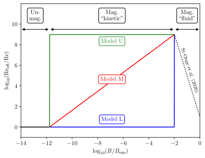
Figure 1: Representation of the different models for the effective Reynolds number for the following values: $n_{e}=10^{-3}\leavevmode\nobreak\ \mathrm{cm}^{-3},\leavevmode\nobreak\ \mathrm{Re}=100,\leavevmode\nobreak\ T=10^{8}\leavevmode\nobreak\ \mathrm{K},\leavevmode\nobreak\ v_{\mathrm{turb}}=300\leavevmode\nobreak\ \mathrm{km}/\mathrm{s},\leavevmode\nobreak\ v_{\mathrm{th},i}=1000\leavevmode\nobreak\ \mathrm{km}/\mathrm{s},\leavevmode\nobreak\ L_{0}=100\leavevmode\nobreak\ \mathrm{kpc}$ and $B_{\mathrm{equ}}=10^{-6}\leavevmode\nobreak\ \mathrm{G}$. In the unmagnetized regime, the solid black line is the Reynolds number that is not modified by the regulation of pressure anisotropies and is given in Eq. (25). Between the limiting magnetic field strengths given in Eqns. (1) and (9), we construct the three different models, Model U, M, and L. The black dotted line corresponds to results obtained from simulations of weakly collisional plasmas presented in St-Onge et al. (2020).

Now, we have to establish the equation that governs the evolution and dynamics of the magnetic field. In this paper, we assume that the magnetic field is amplified by the turbulent dynamo, which consists of the stretching, twisting, and folding of magnetic field lines by turbulent motions (Kazantsev 1968). If we consider the framework of Kolmogorov turbulence, the rate-of-strain tensor is dominated by motions at the viscous scale (Schekochihin & Cowley 2006), which means $|\nabla\boldsymbol{u}|\approx(v_{\mathrm{turb}}/L_{0})\mathrm{Re}^{1/2}$. On the other hand, in a plasma where a Braginskii-type viscosity is assumed, parallel motions to the magnetic field will be damped and only the parallel component of the rate-of-strain tensor $\hat{\boldsymbol{b}}\hat{\boldsymbol{b}}:\nabla\boldsymbol{u}$ is relevant. Therefore, using the induction equation

$$\frac{d\ln B}{dt}=\left(\hat{\boldsymbol{b}}\hat{\boldsymbol{b}}-\overline{\boldsymbol{I}}\right):\nabla\boldsymbol{u},$$ (27)

we obtain

$$\frac{\mathrm{d}\ln B}{\mathrm{d}t}\approx\frac{v_{\mathrm{turb}}}{L_{0}}\mathrm{Re}_{\mathrm{eff}}^{1/2},$$ (28)

where $\mathrm{Re}_{\mathrm{eff}}$ depends on the magnetization state and is given in Fig. 1. We solve Eq. (28) for all magnetization states.

All in all, we constructed $N_{\mathrm{tree}}=10^{3}$ merger trees with $N_{z}=300$ steps between $z=0$ and $z_{\mathrm{max}}$. Once plasma parameters are calculated and averaged according to Eqs. (10) and (12), Eq. (28) is solved between all the redshift steps. Our choice of time resolution between two given redshift steps is explained in detail in Appendix D. Finally, we have adopted the following convention. The magnetic field is assumed to have reached equipartition when its energy density equals at least 90% the density energy of the turbulent velocity field.

4 Results

4.1 Basic plasma parameters from 1D profiles

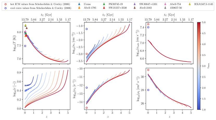
Figure 2: Evolution of various plasma quantities, as a function of redshift, and for different values of $z_{\mathrm{max}}$. Each curve represents the average value of the quantity over $N_{\mathrm{tree}}=10^{3}$ merger trees (see Sec. C) for which a redshift-dependent, one-dimensional profile has been calculated according to Eqs. (10) and (12). The age of the Universe $t_{\mathrm{U}}$ at each redshift is plotted on the second $x$-axis. In order to assess the validity of our model, we have added observations values from a sample of nine clusters for the temperature (see the detailed list in the main text), and estimation from Schekochihin & Cowley (2006) for other quantities.

Figure 2 showcases the temporal evolution of various plasma parameters (Sec. 3.3), for different $z_{\mathrm{max}}$ values associated with merger trees generated using the Modified GALFORM algorithm. Initially, we observe a similarity in the trends of the temperature and turbulent velocity curves. The algorithm demonstrates a decline in these curves, by approximately 10 to 20% of the total runtime, followed by a local minimum and a subsequent steady increase until reaching $z=0$. Additionally, we notice that higher values of $z_{\mathrm{max}}$ lead to steeper local minima. While the underlying cause of these curve shapes remains unclear, we can provide some explanations. Firstly, it is important to note that the merger trees have been constructed with a uniform mass resolution of $M_{\mathrm{res}}=10^{12}\leavevmode\nobreak\ M_{\odot}$, representing a thousandth of the final cluster’s mass. However, the GALFORM algorithm incorporates two stop conditions: either reaching a predetermined value of $z_{\mathrm{max}}$ or the subhaloes reaching the resolution mass during the mass-splitting procedure, regardless of the redshift. Consequently, a higher $z_{\mathrm{max}}$ corresponds to fewer subhaloes in the tree near this redshift. Nonetheless, deviations from the mean values of temperature and turbulent velocity at $z=0$ remain minimal. Furthermore, the concentration parameter $c$ is computed at each node of the tree by considering energy conservation, accounting for accreted matter. When the merger tree extends to higher redshift values, the accretion of additional matter can substantially alter the final value of the concentration parameter, which could explain why $c$-values of the curves with $1\lesssim z_{\mathrm{max}}\lesssim 2$ at $z=0$ are higher. However, it is observed from Fig. 2 that variations in $c$-values at $z=0$ do not seem to impact the electron density curves. Remarkably, the $c$-value converges to approximately $c\simeq 1.2$ for $z\gtrsim 2.5$, being in relatively good agreement with the cMr-relation derived in Biviano et al. (2017).

In the preceding paragraph several concerns regarding the validity of our magnetic field model were raised, as numerical artifacts arise for redshifts close to $z_{\mathrm{max}}$. As previously stated, both the temperature and turbulent velocity curves exhibit a decreasing trend that precedes a global minimum and then displays a constant increase until $z=0$. However, it has been observed that this trend strongly relies on the initial conditions set by $z_{\mathrm{max}}$, resulting in a numerical effect in our model. In order to mitigate the potential impact of these artifacts on our conclusions, we have decided to impose constraints on the value of $z_{\mathrm{max}}$. Fig. 2 clearly indicates that all curves converge towards a common value for redshift values $z\gtrsim 2$. Therefore, we have opted to exclude merger trees with $z_{\mathrm{max}}\leq 2$ for further analysis. Although selecting the merger tree with the highest $z_{\mathrm{max}}$ seems to be a plausible option, it is worth noting that the number of DM subhaloes decreases as $z_{\mathrm{max}}$ increases due to the way the GALFORM algorithm operates. Therefore, from now on, we will only use the merger tree with $z_{\mathrm{max}}=4$ to implement our magnetic field amplification model. Additionally, we initiate the dynamo process at redshift values equal to or below $z_{\mathrm{start}}\leq 2$, ensuring that the influence of the mass resolution remains marginal.

Finally, in order to assess the robustness of our model, we have plotted on Fig. 2 observational values of various physical quantities for nine different clusters. It should be noted that this selection of clusters includes not only clusters in the same dynamical state; some are undergoing merging processes, while others are in a relaxed state. For instance, Miranda et al. (2008) combined X-ray observations and strong lensing analysis of RX J1347.5-1145, and revealed a complex structure. They suggested a merger scenario between DM subclumps that would account for discrepancies with mass estimates from the virial theorem. Moreover, Barrena et al. (2002) provided evidence of a major collision between 1E0657-56 and a subcluster, and Maurogordato et al. (2008) provided optical observations suggesting that Abell 2163 had undergone a recent ($\approx 0.5$ Gyr) collision. For the temperature, we have plotted results from X-ray observations for the Coma cluster, Abell 1795, PKS0745-19, SWJ1557+3530, and SWJ0847+1331 from Moretti et al. (2011) and references therein. We have also plotted the temperature from X-ray observations from Wallbank et al. (2022) for Abell 2163, Abell 754, RX J1347.5-1145, and 1E 0657-56. Our model results in an average temperature at $z=0$ that is in good agreement with most clusters of the observational sample. We also have plotted estimations of the typical values of various physical quantities reported by Schekochihin & Cowley (2006), for both cool cores and hot ICM components of the Hydra A cluster. In conclusion, we can assert that our model is in approximate agreement with observations as long as we aim to model the hot, X-ray-emitting ICM component.

4.2 Magnetic field amplification

In this section, we present the magnetic field amplification obtained from our model that is based on an effective Reynolds number. It is worth recalling that we have integrated our dynamo model into the merger tree with $z_{\mathrm{max}}=4$, and initiated the amplification process at various redshifts between $z_{\mathrm{start}}=2$ and $z_{\mathrm{start}}=0.1$.

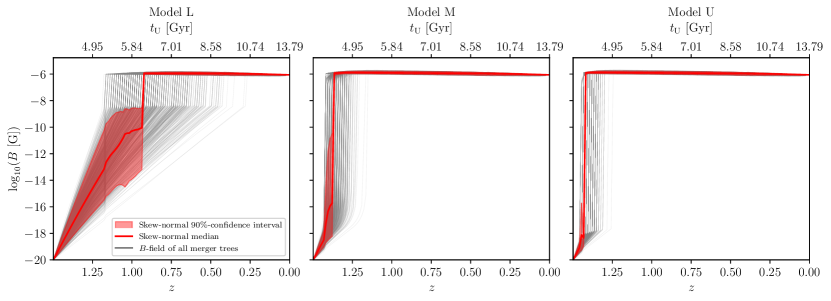
Figure 3: Evolution of the magnetic field, for $\alpha_{0}=20$ and $z_{\mathrm{start}}=1.5$, and for the three models for the effective Reynold number. The area spanned by $N_{\mathrm{tree}}=10^{3}$ merger trees is colored in gray. The red curve indicates the average obtained by fitting all curves at each redshift value with a Skew-normal distribution (see Sec. C). The colored area shows the 90%-confidence interval for such a distribution. The age of the Universe $t_{\mathrm{U}}$ at each redshift is plotted on the second $x$-axis.

4.2.1 Example of magnetic field evolution

Figure 3 shows an example of the magnetic field evolution for the three effective Reynolds number models, detailed in Sec. 3.4, for $\alpha_{0}=20$ (see Eq. (21) for the model of the turbulent forcing scale), $z_{\mathrm{start}}=1.5$, and $B_{0}=10^{-20}\leavevmode\nobreak\ \mathrm{G}$. The gray curves represent the magnetic field evolution of all individual $N_{\mathrm{tree}}=10^{3}$ merger trees. In red, we show the Skew-normal average median with a 90% confidence interval; see Appendix C. Note that the estimated error during the exponential phase of Model L is larger than that of the other models. This can be partially explained by the fact that, in Model L, the Reynolds number is modified by kinetic instabilities only once the magnetic field amplitude reaches the order of $\mathrm{nG}$. Compared to Models M and U, in Model L, the Reynolds number remains at a value several orders of magnitude lower for a longer time, allowing the various curves to spread more until the Reynolds number increases drastically, when $B$ exceeds the threshold given by Eq. (9). In all three cases, Fig. 3 demonstrates that once an amplitude of a few $\mathrm{nG}$ is achieved, the amplification of the magnetic field towards equipartition is nearly instantaneous.

Figure 4 illustrates the time evolution of the magnetic field for the three distinct effective Reynolds number models, detailed in Sec. 3.4, for a specific value of $\alpha_{0}=20$, starting at redshifts of $z_{\mathrm{start}}=0.5$, $1$, and $1.5$.

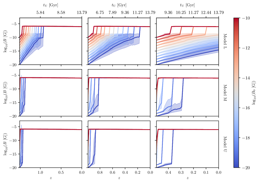
Figure 4: Evolution of the magnetic field amplitude over redshift for different models of effective Reynolds number. The curves and shaded areas correspond respectively to the average and the 90%-confidence interval given by the averaging process described in Sec. C. The age of the Universe $t_{\mathrm{U}}$ at each redshift is plotted on the second $x$-axis. Each row corresponds to a different model, and each column corresponds to a different starting redshift of the dynamo. Model L (top row) has the lowest growth rate, while Models M and U (middle and bottom rows, respectively) show faster growth rates. The figure also shows that the dynamo was much faster in the past (higher redshift values).

Figure 4 illustrates the same evolution of the magnetic field as on Fig. 3, but this time for $z_{\mathrm{start}}=0.5,1,1.5$, and for initial seed field values ranging from $\log_{10}(B\leavevmode\nobreak\ [\mathrm{G}])=-20$ to $-10$. Firstly, it is evident that for models M and U, the curves coincide for $B_{0}\gtrsim 10^{-16}\leavevmode\nobreak\ \mathrm{G}$ and, in particular, the time required to reach equipartition with the turbulent velocity field is independent of $B_{0}$. Therefore, we choose to omit the error bars in our subsequent analyses described below. It also appears that the growth rate of the magnetic field becomes faster as the redshift increases. This effect can only be justified by the evolution of various plasma parameters incorporated in Eq. (28) for the growth rate.

4.2.2 Time to equipartition

Figure 6 shows the minimum redshift $z_{\mathrm{min}}$ at which the dynamo has to start such that equipartition with the turbulent velocity field can be reached, for the three effective Reynolds number models and for various values of $\alpha_{0}$. Firstly, it can be observed that equipartition can be reached in all the different configurations that we have implemented. Moreover, it is clear that Models M and U are indistinguishable for $\log_{10}(B_{0}\leavevmode\nobreak\ [\mathrm{G}])\gtrsim-17$. Furthermore, below these values, the differences between their respective curves are not significant.

The important conclusions that can be drawn from these results are as follows. Firstly, assuming that the modification of effective ion-ion collisionality is the sole physical quantity modified by kinetic instabilities, it can reasonably be accepted that Model L represents a lower limit of $z_{\mathrm{min}}$. Additionally, even though Model U does not represent an upper limit to the effective Reynolds number, it can be assumed that any faster model would not result in any changes to the values presented in Fig. 6. In summary, any effective Reynolds number model lying between the curves associated with Models M and U (Fig. 8) would not influence the dynamics of the magnetic field on cosmological scales. On the other hand, considering a model between the curves L and M would indeed lead to changes in the values of $z_{\mathrm{min}}$ compared to those presented in Fig. 6. Finally, we are limited in the conclusions we can draw due to our simple limitation in modeling the dynamics of the turbulent field, particularly its injection scale. If $\alpha_{0}$ were to evolve, especially through certain mechanisms of turbulent decay, our results would obviously be modified. We leave a more comprehensive modeling of the turbulent velocity field for future work.

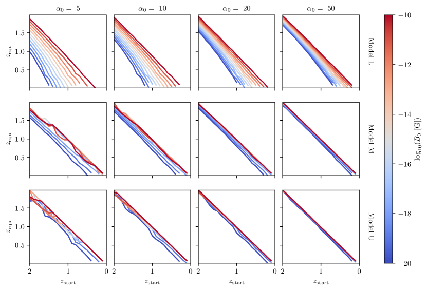
Figure 5: Time required for the magnetic field to reach equipartition with the turbulent velocity field, for different values of the initial magnetic seed field. Each row corresponds to the different models of the effective Reynolds number in the magnetized kinetic regime (Sec. 3.4). Each column corresponds to a different turbulent injection scale.

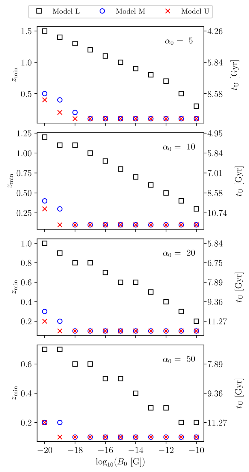
Figure 6: Minimum redshift $z_{\mathrm{min}}$ from which a dynamo has to start to take the magnetic field $B$ up to equipartition with the turbulent velocity field at $z=0$, for different values of the initial magnetic seed field, and for each model for the effective Reynolds number. Each panel corresponds to a specific value of the injection scale defined by Eq. (21). Note that in the upper panel, for Model L, equipartition is never reached for $\log_{10}(B_{0}\leavevmode\nobreak\ [\mathrm{G}])\lesssim-18$.

5 Discussion

Using merger trees has enabled us to study the evolution of certain plasma quantities, including the magnetic field, without relying on computationally expensive simulations. However, such an approach presents a number of uncertainties. Firstly, we have only used the Modified GALFORM algorithm, as it has been calibrated to the mass function of the Millennium simulations. We do not know (yet) if our conclusions would change when considering another merger tree algorithm.

When applying the merger tree algorithm, we have to pay special attention to numerical artifacts. In particular, we have constrained the value of $z_{\mathrm{max}}$ (redshift at which the merging process starts) to $z_{\mathrm{max}}=4$, so that our results are not influenced by numerical effects related to mass resolution (see Fig. 2). Furthermore, we decided to start the dynamo process from $z_{\mathrm{start}}\simeq 2$ or below. Indeed, below $z_{\mathrm{start}}=2$, all curves with $z_{\mathrm{max}}\geq 4$ are approximately identical. Therefore, our ability to study dynamo processes at $z\gtrsim 2$ depends on the model for the concentration parameter considered.

Also, the effective Reynolds number has to be chosen carefully, mainly because Models L and U do not necessarily constitute a lower and upper bound per se. This may be susceptible to introducing biases in the minimum redshift, $z_{\mathrm{min}}$, at which the magnetic field amplification needs to start in order to reach equipartition at $z=0$. However, our results have shown that Models M and U produce nearly identical results. This is not surprising, because even if Models M and U are not the same, they both differ from the classical Reynolds number by (many) orders of magnitude.

Furthermore, confining the evolution of the turbulent injection scale appears to be one of the few necessary conditions to constrain the evolution of the magnetic field. It should be noted that other sources of turbulence are likely to exist during certain phases of the formation of a cluster, potentially with different forcing length scales. Other sources include for example, subcluster and galactic wakes (e.g. Subramanian et al. 2006) and jets from active galactic nuclei (e.g. Fujita et al. 2020).

Finally, for the scenario presented in Fig. 3 for instance, the magnetic field increases by 14 orders of magnitude, while the temperature increases by one order of magnitude. In this specific example, the $\beta$ parameter changes from $\beta\approx 10^{28}$ at $z=1.5$ to $\beta\approx 1$ at $z=0$. Therefore, making use of hydrodynamical simulations seems justified in the kinematic phase. After reaching equipartition, back reactions of the plasma by the magnetic field could be dynamically important.

6 Conclusions

In this work, we used the Modified GALFORM code (Parkinson et al. 2008) to investigate the amplification of magnetic fields in the intracluster medium (ICM) during the formation of galaxy clusters by successive mergers of dark matter halos. We focused on clusters with a typical mass of $M=10^{15}\leavevmode\nobreak\ \mathrm{M}_{\odot}$. To this end, we implemented one-dimensional profiles for the distribution of dark matter, baryonic gas, temperature, and turbulent velocity, assuming spherical symmetry, and following the methodology proposed by Dvorkin & Rephaeli (2011) and Johnson et al. (2021). For a given merger tree realization, the profiles of all subhalos at a given redshift were averaged in order to calculate relevant plasma parameters as a function of redshift. This process has been performed for $N_{\mathrm{tree}}=10^{3}$ merger trees to establish statistical properties. We compared the temperature at $z=0$ obtained from our model with observed values from a sample of selected clusters presented in Moretti et al. (2011) and Wallbank et al. (2022). We also compared other quantities like electron density, turbulent velocity, and ion-ion collision frequency to typical values deduced from Hydra A observations listed in Schekochihin & Cowley (2006). Overall, we found our model to be in good agreement with the observed values from a sample of low-redshift clusters.

We then constructed a semi-analytical model for the amplification of the magnetic field that incorporates the effects of pressure-anisotropy-driven kinetic instabilities (firehose and mirror) for different magnetization regimes (Melville et al. 2016; Rincon et al. 2016; St-Onge & Kunz 2018; St-Onge et al. 2020). Next, we estimated the growth rate of the magnetic field for different values of the strength of the magnetic seed field, and forcing length scales of turbulence. This allowed us to determine the redshift at which equipartition is reached in different scenarios. In practice, we define equipartition as the time when the magnetic energy density reaches at least 90% of the turbulent kinetic energy density. Specifically, for an injection scale of $L_{0}=r_{\mathrm{vir}}/20$, where $r_{\mathrm{vir}}$ is the virial radius of the dark matter halo, the magnetic field evolves in the following way. For our slowest dynamo (effect Reynolds number Model L), the dynamo amplification for seed field values of $\log_{10}(B_{0}\leavevmode\nobreak\ [\mathrm{G}])=-20$ and $-10$ has to start at least from, respectively, $z_{\mathrm{start}}\simeq 1$ and $0.2$ to reach equipartition until the present day. For the other faster scenarios (Models M and U), those values are respectively reduced to $z_{\mathrm{start}}\simeq 0.3$ and $\simeq 0.1$. Although our Model U cannot be considered as an upper limit for the effective Reynolds number, our Model L can constitute a lower limit, provided that the increase of ion-ion collisionality is the sole effect created by the kinetic instabilities to bring the system back to marginal stability.

Overall, our study demonstrates that merger trees can be a valuable tool for constraining the evolution of magnetic fields over cosmological times, particularly in galaxy clusters. In particular, they allow us to probe kinetic plasma effects in the history of the ICM which are inaccessible with state-of-the-art cosmological simulations. Although our approach is not as accurate as fully kinetic plasma simulations, it could potentially constitute a computationally efficient alternative for constraining the dependence of the effective Reynolds number on the magnetic field, in the magnetic “kinetic” regime, when combined with future and more resolved radio observations.

Appendix A GALFORM & Modified GALFORM models

The GALFORM model (Cole et al. 2000) is based upon the extended Press-Schechter theory (Press & Schechter 1974), which considers the following conditional mass function:

$$\begin{split}f(M_{1}|M_{2})d\ln M_{1}=&\sqrt{\frac{2}{\pi}}\frac{\sigma_{1}^{2}(\delta_{1}-\delta_{2})}{(\sigma^{2}-\sigma_{2}^{2})^{3/2}}\\ &\exp\left(-\frac{1}{2}\frac{(\delta_{1}-\delta_{2})^{2}}{\sigma_{1}^{2}-\sigma_{2}^{2}}\right)\left|\frac{d\ln\sigma}{d\ln M_{1}}\right|d\ln M_{1}\end{split}$$ (29)

where $f(M_{1}|M_{2})$ represents the fraction of mass from haloes of mass $M_{2}$ at redshift $z_{2}$ that is contained in progenitor haloes of mass $M_{1}$ at earlier redshift $z_{1}$. The parameter $\delta_{i}$ denotes the linear overdensity threshold for spherical collapse at redshift $z_{i}$. The quantity $\sigma(M)$ denotes the rms linear density fluctuation extrapolated at $z=0$ in spheres containing mass $M$. For simplicity, we adopt $\sigma_{i}(M)\equiv\sigma_{i}$. Taking the limit $z_{1}\to z_{2}$, we get

$$\begin{split}&\left.\frac{df}{dz_{1}}\right|_{z_{1}=z_{2}}d\ln M_{1}dz_{1}\\ &=\sqrt{\frac{2}{\pi}}\frac{\sigma_{1}^{2}}{(\sigma_{1}^{2}-\sigma_{2}^{2})^{3/2}}\frac{d\delta_{1}}{dz_{1}}\left|\frac{d\ln\sigma_{1}}{d\ln M_{1}}\right|d\ln M_{1}dz_{1}\end{split}$$ (30)

which allows obtaining the mean number of haloes of mass $M_{1}$ into which a halo of mass $M_{2}$ splits when we increase redshift upwards with a redshift step $dz_{1}$:

$$\frac{dN}{dM_{1}}=\frac{1}{M_{1}}\frac{df}{dz_{1}}\frac{M_{2}}{M_{1}}dz_{1}.$$ (31)

Assuming a resolution mass $M_{\mathrm{res}}$, we can also determine the average number of progenitors with masses $M_{1}$ in the interval $M_{\mathrm{res}}<M_{1}<M_{2}/2$, which is given by

$$P=\int_{M_{\mathrm{res}}}^{M_{2}/2}\frac{dN}{dM_{1}}dM_{1},$$ (32)

along with the fraction of mass of the final object in progenitors below $M_{\mathrm{res}}$, given by

$$F=\int_{0}^{M_{\mathrm{res}}}\frac{dN}{dM_{1}}\frac{M_{1}}{M_{2}}dM_{1}.$$ (33)

The GALFORM algorithm operates as follows. We start with the redshift and the mass of the final halo. Then we consider a redshift step $dz_{1}$ that satisfies $P\ll 1$ (meaning that a halo is unlikely to have more than two progenitors at redshift $z+dz$). A random number $R\in[0,1]$ is generated. If $R>P$ the main halo is not split, and its mass is reduced to $M_{2}(1-F)$ to account for the accreted mass. If $R\leq P$, then a random mass $M_{\mathrm{res}}>M_{1}>M_{2}/2$ is generated to produce two new haloes with masses $M_{1}$ and $M_{2}(1-F)-M_{1}$. This same process is repeated until the maximum redshift or the resolution mass is reached.

However, there are some issues with such an approach. One of them is that the conditional mass function (29) does not match what is found in $N$-body simulations. However, statistical properties produced by the GALFORM algorithm have similar trends with those of merger trees constructed from high-resolution $N$-body simulations, with an error on mass progenitors that increases with redshift. In that spirit, Parkinson et al. (2008) replaced the initial statistics Eq. (31) with

$$\frac{dN}{dM_{1}}\to\frac{dN}{dM_{1}}G(\sigma_{1}/\sigma_{2},\sigma_{2}/\sigma_{2}),$$ (34)

where $G$ is a ”perturbative” function that matches the generated merger tree with simulations. They also made the following assumption

$$G(\sigma_{1}/\sigma_{2},\sigma_{2}/\sigma_{2})=G_{0}\left(\frac{\sigma_{1}}{\sigma_{2}}\right)^{\gamma_{1}}\left(\frac{\delta_{2}}{\sigma_{2}}\right)^{\gamma_{2}}$$ (35)

for which they obtained $G_{0}=0.57,\gamma_{1}=0.38$ and $\gamma_{2}=-0.01$. Finally, they obtained halo abundances consistent with the Sheth-Tormen mass function (see Parkinson et al. 2008, and references therein). In our work, we use the same values for $G_{0},\gamma_{1}$, and $\gamma_{2}$.

Appendix B Effect number of generated trees

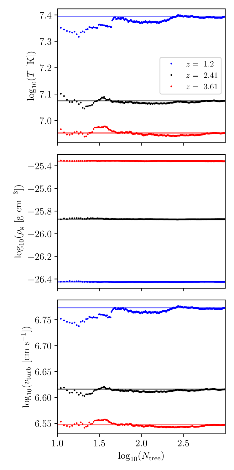
Figure 7: Skew-normal average of the temperature, gas density, and turbulent velocity at three different values of redshift, as a function of the number of generated merger trees. The solid lines represent the values of the physical quantities for $N_{\mathrm{tree}}=10^{3}$.

Figure 7 shows the effect of the number of generated merger trees, on the Skew-normal average (Sec. C) calculated for the temperature, the baryonic gas density, and the turbulent velocity, at three different redshifts. The solid horizontal lines correspond to the value calculated with $N_{\mathrm{tree}}=10^{3}$ merger trees. It is evident that convergence is reached, even for $N_{\mathrm{tree}}\gtrsim 10^{2.5}$ merger trees. This justifies our choice of setting $N_{\mathrm{tree}}=10^{3}$.

Appendix C Skew-normal averaging process

Here we present our method for averaging the time evolution curves of all $N_{\mathrm{tree}}=10^{3}$ merger trees, for all physical quantities. Initially, one might consider using the conventional arithmetic average to estimate the overall behavior of these curves at each specific redshift. However, this approach presents a significant flaw when analyzing the evolution of the magnetic field. By examining the left panel of Fig. 3, it becomes evident that at approximately $z\simeq 0.75$, while a few magnetic field curves have reached equipartition, the majority are still in the phase of exponential growth, with values between $B\approx 10^{-14}$ G and $B\approx 10^{-12}$ G. Consequently, applying the classical arithmetic average to this dataset would yield a value close to equipartition, which does not accurately represent the actual trend exhibited by all the curves.

We decided to adopt the following strategy. At each given redshift, we fit the distribution of the values of all curves with a Skew-normal distribution. However, special attention has to be paid to the magnetic field, as it is shown in Fig. 8. Here, we show the histograms of different quantities, where the $y$-axis is normalized so that the total area of the histogram equals one. The top panel shows the temperature distribution at redshift $z=0.29$, and the middle one the distribution of the magnetic field at the same redshift. If we were to fit the whole magnetic field sample, a skew-normal distribution would not necessarily be suitable as two distinct maxima appear. Therefore, we adopted the following convention. Whenever the number of trees that have reached equipartition is dominant, we fit the region delimited by dashed lines on the middle panel, which is shown on the bottom panel. However, if this number is smaller than the trees outside this region, we fit the trees in the latter. Finally, let us note that the situation where the two histograms, distinguishing the equipartition magnetic field from other values, have the same number of occurrences is extremely rare.

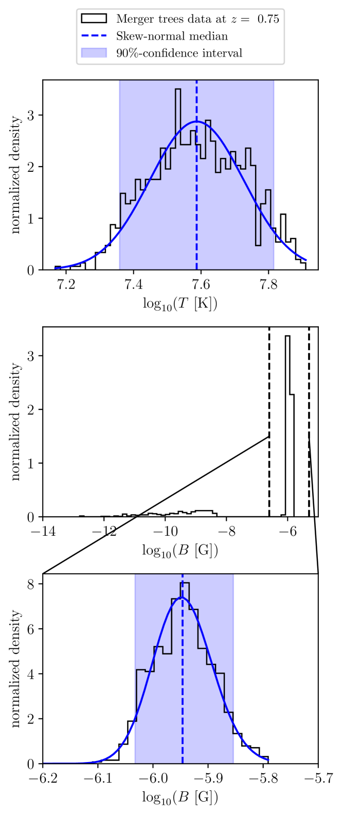
Figure 8: (top) Distribution of the temperature values from all merger trees at redshift $z=0.75$. The blue line represents the Skew-normal distribution used to fit the data. The dashed line and the blue-shaded respectively are the distribution’s median (that is used as an estimator for the average of all curves), and its corresponding 90%-confidence interval. (middle) Distribution of the magnetic field values at this same redshift. The two dashed black lines indicate the region that is fitted with the Skew-normal distribution. (bottom) Fitting of the region in the middle panel. Those three panels were computed with $\mathrm{Re}_{\mathrm{eff}}$ Model L, for $\log_{10}(B_{0}\leavevmode\nobreak\ [\mathrm{G}])=-20$, $\alpha_{0}=20$, and $z_{\mathrm{start}}=1.5$.

Appendix D Time-resolution of the dynamo model

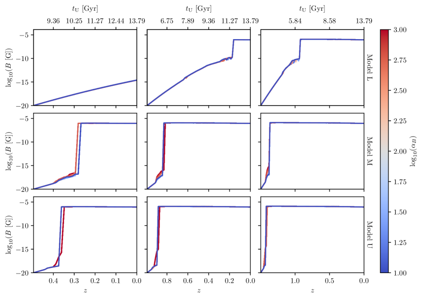
Figure 9: Magnetic field evolution for different values of $\alpha_{B}$. Each column corresponds to a different value of redshift at which the dynamo starts. Each row corresponds to a different model for the effective Reynolds number described in Sec. 3.4.

As described in Sec. 3.4, we solve Eq. (28) between every redshift step of our merger tree (we recall that $N_{z}=300$). Redshift is converted to time using the cosmology calculator of Wright (2006) with the cosmological parameters given in Sec. 3.1. However, considering only the two values of time between two redshift steps is not efficient enough to highlight the complexity of the different stages of the dynamo, like non-linear effects when the magnetic field is getting close to equipartition. Therefore, we create a discretized time grid, between two given redshift steps, whose time step is kept constant (meaning that the number of time grid cells between two different consecutive reshifts will vary). The constant time step is given as follows. We can see that Eq. (28) is of the form $B(t)\propto e^{\Gamma_{\mathrm{eff}}t}$, where $\Gamma_{\mathrm{eff}}\equiv(v_{\mathrm{turb}}/L_{0})\mathrm{Re}_{\mathrm{eff}}^{1/2}$ is the growth rate of the magnetic field. However, given our construction for the effective Reynold number in Sec. 3.4, it is obvious that $\mathrm{Re}_{\mathrm{eff}}\geq\mathrm{Re}$, which would yield a smaller timescale of the growth rate than with the classical Reynold number. Therefore, in order to avoid over-discretizing our grid, we consider the timescale coming from the classical Reynold number, $\Gamma^{-1}$, to be a minimum timescale that should not be exceeded. Therefore, the constant value $\Delta t$ of all grid cells $N_{\Delta t}$ contained in our discretized time between two redshift steps is given by

$$\Delta t\equiv\frac{\Gamma^{-1}}{\alpha_{B}}=\frac{1}{\alpha_{B}}\left(\frac{v_{\mathrm{turb}}}{L_{0}}\mathrm{Re}^{1/2}\right)^{-1},$$ (36)

where $\alpha_{B}$ is a constant value.

We determine the latter by plotting the evolution of the magnetic field, for a fixed set of merger-tree parameters, and for different values of $\alpha_{B}$. Fig. 9 shows such results for $B_{0}=10^{-15}\leavevmode\nobreak\ \mathrm{G}$ and $\alpha_{0}=20$. It appears that when $\alpha_{B}\approx 10^{3.5}$, all curves converge. Therefore, in our work, we adopt a constant value of $\alpha_{B}=10^{4}$. Note that we have checked that this value of $\alpha_{B}$ does not produce other results for all other parameters of $B_{0}$ and $\alpha_{0}$.

Appendix E Estimation of the $c$-parameter

We describe here our method to determine the concentration parameter in every subhalo of the generated merger trees. We start by initiating a value of $c$ for subhalos at $z_{\mathrm{max}}$, with

$$c(M)=4.67\left(\frac{M}{10^{14}h^{-1}M_{\odot}}\right)^{-0.11},$$ (37)

which was proposed by Neto et al. (2007), where $h$ is the Hubble constant in units of $100\leavevmode\nobreak\ \mathrm{km}\leavevmode\nobreak\ \mathrm{s}^{-1}\leavevmode\nobreak\ \mathrm{Mpc}^{-1}$ (see Springel et al. 2005). This choice of the initial condition given in Eq. 37 is somehow arbitrary, but after trying different values of $c$ for the earliest halos, we have found that the final result does not depend on this particular choice. We calculate the total energy of every subhalo using the same expressions adopted in Johnson et al. (2021), which is the sum of its kinetic and potential energy, which are respectively given by

$$T=2\pi\left[r_{\mathrm{vir}}^{3}\rho(r_{\mathrm{vir}})\sigma^{2}(r_{\mathrm{vir}})+\int_{0}^{r_{\mathrm{vir}}}GM(r)\rho(r)r\mathrm{d}r\right]$$ (38)

and

$$W=-\frac{G}{2}\left[\int_{0}^{r_{\mathrm{vir}}}\frac{M^{2}(r)}{r^{2}}\mathrm{d}r+\frac{M^{2}(r_{\mathrm{vir}})}{r_{\mathrm{vir}}}\right].$$ (39)

Here, $\sigma(r)$ is the velocity dispersion that is determined by the Jeans equation:

$$\frac{d(\rho\sigma^{2})}{dr}=-\rho(r)\frac{GM(r)}{r^{2}}.$$ (40)

Therefore, each halo is attributed a total energy of $E_{\mathrm{h}}=T+W$, which depends on parameters $\rho_{\mathrm{s}}$ and $r_{\mathrm{s}}$. When a subhalo is the result of $N$ subhalos merging together, we compute the energy $E_{\mathrm{h,f}}=T_{\mathrm{f}}+W_{\mathrm{f}}$ of the resulting halo, which we equalize with the energy of the system of all progenitors. We express the total energy $E_{N}$ of a system of $N$ subhalos using the same strategy presented in Dvorkin & Rephaeli (2011), which is

$$E_{N}=\sum_{i=1}^{N}E_{\mathrm{h},i}+\sum_{i\neq j}U_{ij}+\sum_{i\neq j}U_{\mathrm{acc},ij}$$ (41)

where

$$U_{ij}\equiv-\frac{GM_{i}M_{j}}{d_{0,ij}}$$ (42)

is the gravitational energy of two halos at the largest point of their separation, with $d_{0,ij}$ being the distance at which subhalos $i$ and $j$ are bound, and where

$$U_{\mathrm{acc},ij}\equiv-\frac{G(M_{i}+M_{j})\Delta M}{r_{\mathrm{vir,f}}}$$ (43)

is the energy component of the accreted matter, where $r_{\mathrm{vir,f}}$ stands for the virial radius of the resulting halo, and where $\Delta M\equiv M_{\mathrm{f}}-\sum_{i}M_{i}$ is the mass that was not resolved during the merging event, below the value of $M_{\mathrm{res}}$. We use the same value of $d_{0}$ as the one adopted in Dvorkin & Rephaeli (2011), which is $d_{0,ij}=5(r_{\mathrm{vir},i}+r_{\mathrm{vir},j})$. Our strategy is then to compute the energy for each subhalo (whether it has one or multiple progenitors) and find the value of $c$ that matches the energy conservation with its progenitors. Once $c$ is calculated, the parameter $\rho_{\mathrm{s}}$ is obtained by integration of the DM density to match the mass of each subhalo.

References

- Adshead et al. (2016) Adshead, P., Giblin, John T., J., Scully, T. R., & Sfakianakis, E. I. 2016, J. Cosmology Astropart. Phys., 2016, 039
- Barrena et al. (2002) Barrena, R., Biviano, A., Ramella, M., Falco, E. E., & Seitz, S. 2002, A&A, 386, 816
- Beck & Wielebinski (2013) Beck, R. & Wielebinski, R. 2013, in Planets, Stars and Stellar Systems. Volume 5: Galactic Structure and Stellar Populations, ed. T. D. Oswalt & G. Gilmore, Vol. 5, 641
- Beresnyak (2012) Beresnyak, A. 2012, Phys. Rev. Lett., 108, 035002
- Biermann (1950) Biermann, L. 1950, Zeitschrift Naturforschung Teil A, 5, 65
- Biviano et al. (2017) Biviano, A., Moretti, A., Paccagnella, A., et al. 2017, A&A, 607, A81
- Bonafede et al. (2010) Bonafede, A., Feretti, L., Murgia, M., et al. 2010, A&A, 513, A30
- Braginskii (1965) Braginskii, S. I. 1965, Reviews of Plasma Physics, 1, 205
- Brandenburg et al. (2023) Brandenburg, A., Rogachevskii, I., & Schober, J. 2023, MNRAS, 518, 6367
- Brandenburg et al. (2017) Brandenburg, A., Schober, J., Rogachevskii, I., et al. 2017, The Astrophysical Journal Letters, 845, L21
- Chandrasekhar et al. (1958a) Chandrasekhar, S., Kaufman, A. N., & Watson, K. M. 1958a, Proceedings of the Royal Society of London Series A, 245, 435
- Chandrasekhar et al. (1958b) Chandrasekhar, S., Kaufman, A. N., & Watson, K. M. 1958b, Proceedings of the Royal Society of London Series A, 245, 435
- Chew et al. (1956) Chew, G. F., Goldberger, M. L., & Low, F. E. 1956, Proceedings of the Royal Society of London Series A, 236, 112
- Cole et al. (2000) Cole, S., Lacey, C. G., Baugh, C. M., & Frenk, C. S. 2000, MNRAS, 319, 168
- Dominguez-Fernández et al. (2019) Dominguez-Fernández, P., Vazza, F., Brüggen, M., & Brunetti, G. 2019, Monthly Notices of the Royal Astronomical Society, 486, 623
- Durrer & Neronov (2013) Durrer, R. & Neronov, A. 2013, A&A Rev., 21, 62
- Dvorkin & Rephaeli (2011) Dvorkin, I. & Rephaeli, Y. 2011, MNRAS, 412, 665
- Ellis et al. (2019) Ellis, J., Fairbairn, M., Lewicki, M., Vaskonen, V., & Wickens, A. 2019, J. Cosmology Astropart. Phys., 2019, 019
- Fitzpatrick (2014) Fitzpatrick, R. 2014, Plasma Physics: An Introduction (Taylor & Francis)
- Fujita et al. (2015) Fujita, T., Namba, R., Tada, Y., Takeda, N., & Tashiro, H. 2015, J. Cosmology Astropart. Phys., 2015, 054
- Fujita et al. (2020) Fujita, Y., Cen, R., & Zhuravleva, I. 2020, MNRAS, 494, 5507
- Gary (1992) Gary, S. P. 1992, J. Geophys. Res., 97, 8519
- Gómez et al. (2022) Gómez, J. S., Padilla, N. D., Helly, J. C., et al. 2022, MNRAS, 510, 5500
- Helander et al. (2016) Helander, P., Strumik, M., & Schekochihin, A. A. 2016, Journal of Plasma Physics, 82, 905820601
- Hellinger (2007) Hellinger, P. 2007, Physics of Plasmas, 14, 082105
- Hubrig et al. (2011) Hubrig, S., Schöller, M., Kharchenko, N. V., et al. 2011, A&A, 528, A151
- Jedamzik & Saveliev (2019) Jedamzik, K. & Saveliev, A. 2019, Phys. Rev. Lett., 123, 021301
- Johnson et al. (2021) Johnson, T., Benson, A. J., & Grin, D. 2021, The Astrophysical Journal, 908, 33
- Joyce & Shaposhnikov (1997) Joyce, M. & Shaposhnikov, M. 1997, Phys. Rev. Lett., 79, 1193
- Kazantsev (1968) Kazantsev, A. P. 1968, Soviet Journal of Experimental and Theoretical Physics, 26, 1031
- Kravtsov & Borgani (2012) Kravtsov, A. V. & Borgani, S. 2012, Annual Review of Astronomy and Astrophysics, 50, 353
- Kulsrud et al. (1997) Kulsrud, R., Cowley, S. C., Gruzinov, A. V., & Sudan, R. N. 1997, Phys. Rep, 283, 213
- Kulsrud (1983) Kulsrud, R. M. 1983, in Handbook of plasma physics. Vol. 1: Basic plasma physics I., ed. A. A. Galeev & R. N. Sudan, 115–144
- Kunz et al. (2014) Kunz, M. W., Schekochihin, A. A., & Stone, J. M. 2014, Phys. Rev. Lett., 112, 205003
- Maurogordato et al. (2008) Maurogordato, S., Cappi, A., Ferrari, C., et al. 2008, A&A, 481, 593
- McCarthy et al. (2007) McCarthy, I. G., Bower, R. G., & Balogh, M. L. 2007, MNRAS, 377, 1457
- Melville et al. (2016) Melville, S., Schekochihin, A. A., & Kunz, M. W. 2016, MNRAS, 459, 2701
- Mikhailov & Andreasyan (2021) Mikhailov, E. A. & Andreasyan, R. R. 2021, Open Astronomy, 30, 127
- Miniati & Beresnyak (2015) Miniati, F. & Beresnyak, A. 2015, Nature, 523, 59
- Miranda et al. (2008) Miranda, M., Sereno, M., de Filippis, E., & Paolillo, M. 2008, MNRAS, 385, 511
- Mogavero & Schekochihin (2014) Mogavero, F. & Schekochihin, A. A. 2014, MNRAS, 440, 3226
- Moretti et al. (2011) Moretti, A., Gastaldello, F., Ettori, S., & Molendi, S. 2011, A&A, 528, A102
- Navarro et al. (1996) Navarro, J. F., Frenk, C. S., & White, S. D. M. 1996, ApJ, 462, 563
- Neto et al. (2007) Neto, A. F., Gao, L., Bett, P., et al. 2007, MNRAS, 381, 1450
- Ostriker et al. (2005) Ostriker, J. P., Bode, P., & Babul, A. 2005, ApJ, 634, 964
- Parker (1958) Parker, E. N. 1958, Physical Review, 109, 1874
- Parkinson et al. (2008) Parkinson, H., Cole, S., & Helly, J. 2008, MNRAS, 383, 557
- Planck Collaboration et al. (2016) Planck Collaboration, Ade, P. A. R., Aghanim, N., et al. 2016, A&A, 594, A19
- Planck Collaboration et al. (2020) Planck Collaboration, Aghanim, N., Akrami, Y., et al. 2020, A&A, 641, A6
- Press & Schechter (1974) Press, W. H. & Schechter, P. 1974, ApJ, 187, 425
- Quashnock et al. (1989) Quashnock, J. M., Loeb, A., & Spergel, D. N. 1989, ApJ, 344, L49
- Rincon (2019) Rincon, F. 2019, Journal of Plasma Physics, 85, 205850401
- Rincon et al. (2016) Rincon, F., Califano, F., Schekochihin, A. A., & Valentini, F. 2016, Proceedings of the National Academy of Science, 113, 3950
- Riquelme et al. (2015) Riquelme, M. A., Quataert, E., & Verscharen, D. 2015, ApJ, 800, 27
- Rudakov & Sagdeev (1961) Rudakov, L. I. & Sagdeev, R. Z. 1961, Soviet Physics Doklady, 6, 415
- Santos-Lima et al. (2014) Santos-Lima, R., de Gouveia Dal Pino, E. M., Kowal, G., et al. 2014, ApJ, 781, 84
- Schekochihin & Cowley (2006) Schekochihin, A. A. & Cowley, S. C. 2006, Physics of Plasmas, 13, 056501
- Schekochihin et al. (2002) Schekochihin, A. A., Cowley, S. C., Hammett, G. W., Maron, J. L., & McWilliams, J. C. 2002, New Journal of Physics, 4, 84
- Schekochihin et al. (2004) Schekochihin, A. A., Cowley, S. C., Taylor, S. F., Maron, J. L., & McWilliams, J. C. 2004, The Astrophysical Journal, 612, 276
- Scherrer et al. (1977) Scherrer, P. H., Wilcox, J. M., Svalgaard, L., et al. 1977, Solar Physics, 54, 353
- Schleicher et al. (2013) Schleicher, D. R. G., Schober, J., Federrath, C., Bovino, S., & Schmidt, W. 2013, New Journal of Physics, 15, 023017
- Schmassmann et al. (2018) Schmassmann, M., Schlichenmaier, R., & Bello González, N. 2018, A&A, 620, A104
- Schober et al. (2022) Schober, J., Rogachevskii, I., & Brandenburg, A. 2022, Phys. Rev. Lett., 128, 065002
- Sharma et al. (2006) Sharma, P., Hammett, G. W., Quataert, E., & Stone, J. M. 2006, ApJ, 637, 952
- Shi et al. (2018) Shi, X., Nagai, D., & Lau, E. T. 2018, MNRAS, 481, 1075
- Snyder et al. (1997) Snyder, P. B., Hammett, G. W., & Dorland, W. 1997, Physics of Plasmas, 4, 3974
- Southwood & Kivelson (1993) Southwood, D. J. & Kivelson, M. G. 1993, J. Geophys. Res., 98, 9181
- Springel et al. (2005) Springel, V., White, S. D. M., Jenkins, A., et al. 2005, Nature, 435, 629
- St-Onge & Kunz (2018) St-Onge, D. A. & Kunz, M. W. 2018, ApJ, 863, L25
- St-Onge et al. (2020) St-Onge, D. A., Kunz, M. W., Squire, J., & Schekochihin, A. A. 2020, Journal of Plasma Physics, 86, 905860503
- Subramanian et al. (2006) Subramanian, K., Shukurov, A., & Haugen, N. E. L. 2006, MNRAS, 366, 1437
- Talebian et al. (2020) Talebian, A., Nassiri-Rad, A., & Firouzjahi, H. 2020, Phys. Rev. D, 102, 103508
- Törnkvist (1998) Törnkvist, O. 1998, Phys. Rev. D, 58, 043501
- Tweed et al. (2009) Tweed, D., Devriendt, J., Blaizot, J., Colombi, S., & Slyz, A. 2009, A&A, 506, 647
- Vazza et al. (2012) Vazza, F., Roediger, E., & Brüggen, M. 2012, A&A, 544, A103
- Vogt & Enßlin (2003) Vogt, C. & Enßlin, T. A. 2003, A&A, 412, 373
- Wallbank et al. (2022) Wallbank, A. N., Maughan, B. J., Gastaldello, F., Potter, C., & Wik, D. R. 2022, MNRAS, 517, 5594
- Wright (2006) Wright, E. L. 2006, PASP, 118, 1711
Acknowledgements.
We are grateful to Jonathan Squire and Matthew W. Kunz for very useful discussions on weakly collisional plasmas. We further thank Abhijit B. Bendre for his numerous comments on this study. Finally, we acknowledge the support from the Swiss National Science Foundation under Grant No. 185863.Appendix A GALFORM & Modified GALFORM models