No distributed quantum advantage for approximate graph coloring

Xavier Coiteux-Roy  $\cdot$  School of Computation, Information and Technology, Technical University of Munich, Germany  $\cdot$  Munich Center for Quantum Science and Technology, Germany

Francesco d’Amore  $\cdot$  Aalto University, Finland

Rishikesh Gajjala  $\cdot$  Aalto University, Finland  $\cdot$  Indian Institute of Science, India

Fabian Kuhn  $\cdot$  University of Freiburg, Germany

François Le Gall  $\cdot$  Nagoya University, Japan

Henrik Lievonen  $\cdot$  Aalto University, Finland

Augusto Modanese  $\cdot$  Aalto University, Finland

Marc-Olivier Renou  $\cdot$  Inria, Université Paris-Saclay, Palaiseau, France  $\cdot$  CPHT, Ecole Polytechnique, Institut Polytechnique de Paris, Palaiseau, France

Gustav Schmid  $\cdot$  University of Freiburg, Germany

Jukka Suomela  $\cdot$  Aalto University, Finland

Abstract. We give an almost complete characterization of the hardness of $c$-coloring $\chi$-chromatic graphs with distributed algorithms, for a wide range of models of distributed computing. In particular, we show that these problems do not admit any distributed quantum advantage. To do that:

1. We give a new distributed algorithm that finds a $c$-coloring in $\chi$-chromatic graphs in $\tilde{\mathcal{O}}(n^{\frac{1}{\alpha}})$ rounds, with $\alpha=\bigl{\lfloor}\frac{c-1}{\chi-1}\bigr{\rfloor}$.

2. We prove that any distributed algorithm for this problem requires $\Omega(n^{\frac{1}{\alpha}})$ rounds.

Our upper bound holds in the classical, deterministic $\mathsf{LOCAL}$ model, while the near-matching lower bound holds in the non-signaling model. This model, introduced by Arfaoui and Fraigniaud in 2014, captures all models of distributed graph algorithms that obey physical causality; this includes not only classical deterministic $\mathsf{LOCAL}$ and randomized $\mathsf{LOCAL}$ but also $\mathsf{quantum}$-$\mathsf{LOCAL}$, even with a pre-shared quantum state.

We also show that similar arguments can be used to prove that, e.g., 3-coloring 2-dimensional grids or $c$-coloring trees remain hard problems even for the non-signaling model, and in particular do not admit any quantum advantage. Our lower-bound arguments are purely graph-theoretic at heart; no background on quantum information theory is needed to establish the proofs.

1 Introduction

In this work, we settle the distributed computational complexity of approximate graph coloring, for deterministic, randomized, and quantum versions of the $\operatorname{\mathsf{LOCAL}}$ model of distributed computing.

In brief, the setting is this: We have an input graph $G$ with $n$ nodes. Each node is a computer and each edge represents a communication link. Computation proceeds in synchronous rounds: each node sends a message to each of its neighbors, receives a message from each of its neighbors, and updates its own state. After $T$ rounds, each node has to stop and announce its own output, and the outputs have to form a proper $c$-coloring of the input graph $G$. If the chromatic number of $G$ is $\chi$, in this setting it is trivial to find a $\chi$-coloring in $T=\mathcal{O}(n)$ rounds, as in $\mathcal{O}(n)$ rounds all nodes can learn the full topology of their own connected component and they can locally find an optimal coloring by brute force without any further communication. But the key questions are: How well can we color graphs in $T\ll n$ rounds? And how much does it help if we use quantum computers that can exchange quantum information, possibly with a pre-shared entangled state?

1.1 Main result

We show that for all constants $c$, $\chi$, and $\alpha$, it is possible to find a $c$-coloring of a $\chi$-colorable graph in $T=\tilde{\mathcal{O}}(n^{1/\alpha})$ communication rounds if and only if

$$\alpha\leq\left\lfloor\frac{c-1}{\chi-1}\right\rfloor.$$

For example, if the graph is bipartite ($\chi=2$), this means that the complexity of $2$-coloring is $\tilde{\Theta}(n)$ rounds, $3$-coloring is $\tilde{\Theta}(\sqrt{n})$ rounds, and $4$-coloring is $\tilde{\Theta}(n^{1/3})$ rounds. Here we use $\tilde{\mathcal{O}}$ and $\tilde{\Theta}$ to hide polylogarithmic factors, that is, our results are tight up to polylogarithmic factors.

Perhaps the biggest surprise is that this result holds for a wide range of models of distributed computing: the answer is the same for deterministic, randomized, and quantum versions of the $\operatorname{\mathsf{LOCAL}}$ model, and it holds even if the algorithm has access to shared randomness or pre-shared quantum state (as long as the quantum state is prepared before we reveal the structure of graph $G$).

In particular, we show that there is no distributed quantum advantage for approximate graph coloring in the context of the $\operatorname{\mathsf{LOCAL}}$ model, at least up to polylogarithmic factors.

1.2 Significance and motivation

Our work is directly linked to two lines of research: understanding the quantum advantage in distributed settings, and the complexity of distributed graph coloring in classical settings.

Distributed quantum advantage.

There is a long line of work [27, 46, 54, 67, 65, 42, 21, 43, 4] on quantum advantage in the $\operatorname{\mathsf{CONGEST}}$ model—this is a bandwidth-limited version of the $\operatorname{\mathsf{LOCAL}}$ model. However, much less is known about quantum advantage in the $\operatorname{\mathsf{LOCAL}}$ model.

Earlier work by [33] and [6] on $\operatorname{\mathsf{quantum-LOCAL}}$ brought primarily bad news: they showed that many classical $\operatorname{\mathsf{LOCAL}}$ model lower bounds still hold in the $\operatorname{\mathsf{quantum-LOCAL}}$ model. The quantum advantage demonstrated by [33] was limited to constant factors or required pre-shared quantum resources. The major breakthrough was the recent work by [47] that demonstrated that there is a problem that can be solved in only $2$ rounds using quantum communication, whereas solving it in the classical setting requires $\Omega\!\left(n\right)$ rounds.

However, the problem from [47] is very different from the classical problems commonly studied in the field of distributed graph algorithms, and most importantly, it is not a locally checkable problem. Locally checkable problems are graph problems in which the task is to find a feasible solution subject to local constraints—perhaps the best-known example of such a problem is graph coloring. A lot of recent work on the classical $\operatorname{\mathsf{LOCAL}}$ model has focused on locally checkable problems, and there is nowadays a solid understanding of the landscape of the distributed computational complexity of such problems for the classical models—see, e.g., [11, 9, 24, 35, 10, 30, 61, 19, 22, 36, 8, 18]. However, what is wide open is how $\operatorname{\mathsf{quantum-LOCAL}}$ changes the picture.

A major open problem is whether there is any locally checkable graph problem that can be solved asymptotically faster in $\operatorname{\mathsf{quantum-LOCAL}}$ in comparison with the classical randomized $\operatorname{\mathsf{LOCAL}}$ model, and it has been conjectured that no such problem exists [63]. In this work we provide more evidence in support of this conjecture: we show that various problems related to graph coloring do not admit any significant quantum advantage.

Hardness of distributed coloring.

In a very recent work, [2] studied the notion of locality in three different settings: distributed, dynamic, and online graph algorithms. They showed that for locally checkable problems in rooted regular trees the three notions of locality coincide, but more generally the notions are distinct. The prime example of a problem that separates the models is $3$-coloring bipartite graphs: the distributed locality (i.e., round complexity) of the problem is $\Omega(\sqrt{n})$ [20], but the online locality is $\mathcal{O}(\log n)$ [2]. While this demonstrates that there is large gap between distributed and online settings, this also highlights a blind spot in our understanding of seemingly elementary questions in the classical $\operatorname{\mathsf{LOCAL}}$ model: What, exactly, is the distributed complexity of $3$-coloring bipartite graphs? Can we solve it in $\tilde{\mathcal{O}}(\sqrt{n})$ rounds? And, more generally, what is the distributed complexity of $c$-coloring $\chi$-colorable graphs?

Given the prominent role graph coloring plays in distributed graph algorithms, the state of the art is highly unsatisfactory—the upper and lower bounds are far from each other, even if we consider the seemingly elementary question of coloring bipartite graphs:

• As mentioned above, the complexity of $3$-coloring bipartite graphs is known to be somewhere between $\Omega(\sqrt{n})$ and $\mathcal{O}(n)$. [20] show that $3$-coloring $2$-dimensional grids requires $\Omega(\sqrt{n})$ rounds, and even though they study toroidal grids (which are not necessarily bipartite), the same result can be adapted to also show that $3$-coloring bipartite graphs requires $\Omega(\sqrt{n})$ rounds. It is not known if this is tight; to the best of our knowledge, there is no upper bound other than the trivial $\mathcal{O}(n)$-round algorithm.

• The complexity of $4$-coloring bipartite graphs is only known to be somewhere between $\Omega(\log{n})$ and $\mathcal{O}(n)$. linial1992’s [49] lower bound for coloring trees applies, so we know that the complexity has to be at least $\Omega(\log n)$, but beyond that very little is known. The lower bound construction from [20] cannot be used here since it is easy to $4$-color grids. To come up with a nontrivial upper bound, it would be tempting to use network decompositions in the spirit of [12], but we are lacking network decomposition algorithms with suitable parameters, and in any case this approach cannot produce $4$-colorings or $5$-colorings in $o(\sqrt{n})$ rounds.

In this work we solve all these open questions, up to polylogarithmic factors, for the general task of $c$-coloring $\chi$-colorable graphs. We show that there is plenty of room for improvement in both upper and lower bounds. For example, in the case of $4$-coloring bipartite graphs, the right bound turns out to be $\tilde{\Theta}(n^{1/3})$, which is far from what can be achieved with the state of the art outlined above.

1.3 Contributions in more detail

We will now describe all of our results and contributions in more detail; we refer to Section 2 for an overview of the proof ideas and to Sections 4 and 5 for the proofs.

1.3.1 Classical upper bound (Section 4)

Let us start with the upper bound. We design new distributed algorithms with the following properties:

Theorem 1.1.

There exists a $\operatorname{\mathsf{det-LOCAL}}$ algorithm $\mathcal{A}_{\operatorname{\mathsf{det}}}$ and a $\operatorname{\mathsf{rand-LOCAL}}$ algorithm $\mathcal{A}_{\operatorname{\mathsf{rand}}}$ that, given a parameter $\alpha\in\mathbb{N}$, find a proper vertex coloring with $\alpha(\chi-1)+1$ colors in any graph with chromatic number $\chi$, as follows:

• $\mathcal{A}_{\operatorname{\mathsf{det}}}$ runs in $\mathcal{O}\bigl{(}n^{1/\alpha}\log^{3-1/\alpha}n\bigr{)}\cdot(\log\log n)^{\mathcal{O}(1)}$ rounds.

• $\mathcal{A}_{\operatorname{\mathsf{rand}}}$ runs in $\mathcal{O}\bigl{(}n^{1/\alpha}\log^{2-1/\alpha}n\bigr{)}$ rounds and succeeds with probability $1-1/\poly(n)$.

We note that the algorithms do not need to know $\chi$; it is sufficient to know $\alpha$ and $n$. As a corollary, we can, e.g., $3$-color bipartite graphs in $\tilde{\mathcal{O}}(\sqrt{n})$ rounds by setting $\alpha=2$.

The number of colors $c=\alpha(\chi-1)+1$ may look like a rather unnatural expression, and there does not seem to be a priori any reason to expect that this would be tight—however, as we will see, this is indeed exactly the right number.

1.3.2 Non-signaling model

Our main goal is to show that the algorithms in Theorem 1.1 are optimal (up to polylogarithmic factors), not only in the classical models but also in, e.g., all reasonable variants of the $\operatorname{\mathsf{quantum-LOCAL}}$ model. To this end, we work in the non-signaling model, as defined by [6]; this is essentially equivalent to the $\varphi$$\operatorname{\mathsf{-LOCAL}}$ model defined earlier by [33].

The non-signaling model is a characterization of output distributions that do not violate the no-signaling from the future principle or, equivalently, the causality principle [25]. To better understand this, suppose we have some classical $\operatorname{\mathsf{rand-LOCAL}}$ algorithm $\mathcal{A}$ that runs in $T$ rounds and outputs a vertex coloring. Let $p(G)$ be the output distribution of $\mathcal{A}$ when run on a graph $G$. The key observation is that this distribution is not arbitrary—in particular, it must satisfy the following property:

Definition 1.2 (Non-signaling distribution, informal version).

The output distribution $p(G)$ of $\mathcal{A}$ is non-signaling beyond distance $T$ if the following holds: Let $V$ be a set of nodes of a graph $G$ with $\lvert V\rvert=n$. Fix a subset of nodes $U\subseteq V$ and consider $p(G){\restriction_{U}}$, the restriction of $p(G)$ to $U$. Let $G[U,T]$ be the graph induced by the radius-$T$ neighborhood of $U$ in $G$. Now modify $G$ outside $G[U,T]$ to obtain a different $n$-node graph $G^{\prime}$ while preserving $G[U,T]=G^{\prime}[U,T]$. Then $p(G){\restriction_{U}}=p(G^{\prime}){\restriction_{U}}$.

Put otherwise, changes more than distance $T$ away from $U$ cannot influence the output distribution of $U$. It is not hard to see that this holds for $\operatorname{\mathsf{det-LOCAL}}$ and $\operatorname{\mathsf{rand-LOCAL}}$, even if the algorithm has access to shared randomness. But what makes this notion particularly useful is that it is satisfied also by the $\operatorname{\mathsf{quantum-LOCAL}}$ model, even with a pre-shared quantum state [6, 33]. Informally, a system that violates the non-signaling property would violate causality and enable faster-than-light communication, which is something that quantum physics does not allow.

We use $\operatorname{\mathsf{NS-LOCAL}}$ to refer to the non-signaling model. We say that $\mathcal{A}$ is an $\operatorname{\mathsf{NS-LOCAL}}$ algorithm that runs in $T$ rounds if it produces an output distribution that is non-signaling beyond distance $T$. We will then prove statements of the form “any $\operatorname{\mathsf{NS-LOCAL}}$ algorithm for this problem requires at least $T$ rounds.” As a corollary, this gives a $T$-round lower bound for $\operatorname{\mathsf{det-LOCAL}}$, $\operatorname{\mathsf{rand-LOCAL}}$, and $\operatorname{\mathsf{quantum-LOCAL}}$, even if we have access to shared randomness and pre-shared quantum states. This also puts limits on the existence of so-called finitely dependent colorings [40, 39].

1.3.3 Non-signaling lower bounds (Section 5)

The precise version of our lower bound result states that, for every large enough number of nodes $n$, there exists a $\chi$-chromatic graph on $n$ nodes that is hard to color in $\operatorname{\mathsf{NS-LOCAL}}$.

Theorem 1.3.

Let $\chi\geq 2$, $c\geq\chi$ be integers, and let $\alpha=\lfloor\frac{c-1}{\chi-1}\rfloor$. Let $\varepsilon\in(0,\frac{\alpha-1}{\alpha})$ be a real value, and let $n\in\mathbb{N}$ with

$$n\geq\left\lceil\frac{\log\varepsilon^{-1}}{\log(1+\frac{1}{\alpha})}\right\rceil\cdot\frac{(6\chi+1)^{\alpha+1}-1}{6}.$$

Suppose $\mathcal{A}$ is an $\operatorname{\mathsf{NS-LOCAL}}$ algorithm for $c$-coloring graphs in the family $\mathcal{F}$ of $\chi$-chromatic graphs of $n$ nodes with success probability $q>\varepsilon$. Then the running time of $\mathcal{A}$ is at least

$$T=\Omega\Biggl{(}\frac{1}{\chi^{1+\frac{1}{\alpha}}}\cdot\biggl{(}\frac{n}{\log\varepsilon^{-1}}\biggr{)}^{\frac{1}{\alpha}}\Biggr{)}.$$

A key observation is that, if the parameters $\chi$, $c$, and $\varepsilon$ in Theorem 1.3 are constants, then $T=\Omega(n^{\frac{1}{\alpha}})$, which matches the upper bound in Theorem 1.1 up to polylogarithmic factors. In particular, there is at best polylogarithmic room for any distributed quantum advantage.

While Theorem 1.3 implies bounds for coloring bipartite graphs in general, we will also use our techniques to prove bounds for specific bipartite graphs. By prior work, it is known that $3$-coloring $2$-dimensional grids is hard in the $\operatorname{\mathsf{det-LOCAL}}$ model [20, 1]. We show that this also holds for the non-signaling model:

Theorem 1.4.

Let $\varepsilon\in(0,\frac{3}{4})$ and $N=\lceil\log(\varepsilon^{-1})/\log(\frac{4}{3})\rceil$. Let $n_{1},n_{2}\in\mathbb{N}$ with $\lfloor\frac{n_{1}}{N}\rfloor\geq 5\text{ and }\lfloor\frac{n_{2}}{N}\rfloor\geq 5.$ Suppose $\mathcal{A}$ is an $\operatorname{\mathsf{NS-LOCAL}}$ algorithm that 3-colors $n_{1}\times n_{2}$ grids with probability $q>\varepsilon$. Then, the running time of $\mathcal{A}$ is at least

$$T=\Omega\biggl{(}\frac{\min(n_{1},n_{2})}{\log\varepsilon^{-1}}\biggr{)}.$$

This result is easiest to interpret in the case of a square grid, i.e., $n_{1}=n_{2}$. Then the lower bound (for constant $\varepsilon$) is simply $\Omega(\sqrt{n})$, where $n=n_{1}\cdot n_{2}$, and this is trivially tight since the diameter of the grid is $\mathcal{O}(\sqrt{n})$; hence the problem can be solved in $\mathcal{O}(\sqrt{n})$ rounds with a $\operatorname{\mathsf{det-LOCAL}}$ algorithm. In particular, there is no room for distributed quantum advantage (beyond possibly constant factors).

Finally, we revisit the classical result by [49] about the hardness of coloring trees. We show that essentially the same lower bound holds in the non-signaling model:

Theorem 1.5.

Let $c\geq 2$ be an integer, and $\varepsilon\in(0,1)$. Suppose $\mathcal{A}$ is an $\operatorname{\mathsf{NS-LOCAL}}$ algorithm that $c$-colors trees of size $n\in\mathbb{N}$ with probability $q>\varepsilon$. Then, for infinitely many $n$, as long as $\varepsilon>e^{-n}$, the running time of $\mathcal{A}$ is at least

$$T=\Omega\bigl{(}\log_{c}n-\log_{c}\log\varepsilon^{-1}\bigr{)}.$$

2 Key new ideas and techniques

In this section, we will give an informal overview of the key new ideas and techniques that we use to prove Theorems 1.1, 1.3, 1.4, LABEL: and 1.5. We refer to Sections 4 and 5 for the formal proofs.

2.1 Classical upper bound (Section 4)

Background and prior work.

The only existing distributed algorithm for solving the approximate coloring problem in general graphs that we are aware of is a folklore algorithm based on network decompositions [7, 50]. For parameters $\alpha$ and $d$, an $(\alpha,d)$-network decomposition is a partition of the nodes $V$ of a graph $G=(V,E)$ into clusters of (weak) diameter at most $d$ together with a proper $\alpha$-coloring of the cluster graph; recall that the weak diameter of a cluster $C\subseteq V$ is the maximum distance in $G$ between any two nodes in $C$.

Given such a decomposition, it is not hard to see how to color graphs of chromatic number $\chi$ with $\alpha\chi$ colors in $d$ rounds by using disjoint color palettes for clusters of different colors: For every $i\in[\alpha]$, the nodes in a cluster of color $i$ use colors from the palette $\{i,\alpha+i,2\alpha+i,\dotsc\}$. Each such cluster $C$ is colored by having a leader node collect the entire topology of the cluster and then brute forcing an optimal coloring $\varphi_{C}$ of the cluster. Since the graph has chromatic number $\chi$, coloring $\varphi_{C}$ uses at most $\chi$ colors. Finally, the leader broadcasts the coloring and assigns each node $v$ in $C$ the color $\alpha(\varphi_{C}(v)-1)+i$. This results in a proper coloring with at most $\alpha\chi$ colors. In addition, the nodes do not require knowledge of $\chi$ in advance. This algorithm has for example been used by [12] to compute a non-trivial approximate coloring in a constant number of rounds. Our algorithm is based on two new ideas that are outlined below.

New ingredient 1: New network decomposition algorithms.

Network decomposition algorithms mostly focus on optimizing the product of $\alpha$ and $d$ (as most applications of network decompositions require time proportional to $\alpha d$) or on minimizing the number of cluster colors for a given maximum cluster diameter (e.g., [7, 50, 12, 61, 34]). We are interested in network decompositions with a fixed number of cluster colors $\alpha$ that is beyond our control and where we wish to optimize the value of $d$. By using existing clustering techniques [57, 23, 61, 34] with some minor adaptations, we give randomized and deterministic algorithms that, for any parameter $\varepsilon>0$, compute a set of non-adjacent clusters such that the cluster diameter of each cluster is $\polylog(n)/\varepsilon$ and the total number of unclustered nodes is at most $\varepsilon n$. For every integer $\alpha$, this can in turn be used to compute an $(\alpha,d)$-network decomposition with $d=\tilde{\mathcal{O}}(n^{1/\alpha})$.

Let us illustrate the idea for the case $\alpha=2$. Setting $\varepsilon=1/\sqrt{n}$, we compute a set of non-adjacent clusters of diameter $\tilde{\mathcal{O}}(\sqrt{n})$ such that at most $\mathcal{O}(\sqrt{n})$ nodes remain unclustered. The constructed clusters can all be colored with color $1$ and the connected components of the unclustered nodes form the clusters of color $2$. We thus obtain a $(2,\tilde{\mathcal{O}}(\sqrt{n}))$-network decomposition in time $\tilde{\mathcal{O}}(\sqrt{n})$ and one can therefore color graphs of chromatic number $\chi$ with $2\chi$ colors in $\tilde{\mathcal{O}}(\sqrt{n})$ rounds.

New ingredient 2: The hiding trick.

In Section 4 we show how to reduce the number of colors used while keeping the round complexity the same. The main new idea is what we call the hiding trick: First we make sure that clusters of the same color are at least four hops apart; this can be achieved by running a network decomposition protocol on $G^{3}$. For simplicity, assume that we have a $(2,\tilde{\mathcal{O}}(\sqrt{n}))$-network decomposition. Let $C$ be a cluster of color $1$. We first extend $C$ to an extended cluster $C_{1}$ that includes all unclustered nodes that are adjacent to $C$. Next we find a proper $\chi$-coloring of $C_{1}$ using colors $\{1,\dotsc,\chi\}$ by brute force. Finally, any boundary node of $C_{1}$ that has color $\chi$ is removed, thus yielding a cluster $C_{0}$ with $C\subseteq C_{0}\subseteq C_{1}$. Note that $C_{0}$ is colored using at most $\chi$ colors and that and all boundary nodes of $C_{0}$ have a color different from $\chi$. We have effectively hidden the color $\chi$ inside the cluster. Now we continue with the rest of the process and can safely use colors $\{\chi,\dotsc,2\chi-1\}$ to color the uncolored nodes in clusters of color $2$. The end result is a proper $(2\chi-1)$-coloring, and the running time is simply a constant times the cluster diameter $d=\tilde{\mathcal{O}}(\sqrt{n})$. With this strategy, for instance, we can compute a $3$-coloring of bipartite graphs in $\tilde{\mathcal{O}}(\sqrt{n})$ rounds.

Theorem 1.1 is in essence a formalization and generalization of the hiding trick. We can hide one color in each cluster and therefore reuse one of the colors for all of the $\alpha$ cluster colors. This results in a coloring with $\alpha(\chi-1)+1$ colors. In addition, if one chooses the color palettes carefully, it is not necessary for the nodes to know $\chi$ beforehand. At first this may seem like an ad-hoc trick that cannot possibly be optimal—after all, we are saving only one color in each step. However, our matching lower bound shows that the hiding trick is essentially the best that we can do in distributed coloring, even if we have access to quantum resources.

2.2 Non-signaling lower bounds (Section 5)

Prior work on classical lower bounds.

As a warm-up, let us first see how one could prove a lower bound similar to Theorem 1.3 for classical models. For concreteness, let us focus on the case $\chi=2$ and $c=3$ in the $\operatorname{\mathsf{det-LOCAL}}$ model. Then $\alpha=2$, and we would like to show that $3$-coloring bipartite graphs requires $\Omega(\sqrt{n})$ rounds.

Here we can make use of existential graph-theoretic arguments similar to the one already used by [49]. Let $\mathcal{A}$ be a $\operatorname{\mathsf{det-LOCAL}}$ algorithm that purportedly finds a $3$-coloring in bipartite graphs in $T(n)=o(\sqrt{n})$ rounds. Now suppose that we are able to construct a graph $G$ on $n$ nodes with the following properties:

1. $G$ is locally bipartite: for any node $v$ of $G$, the subgraph of $G$ induced by the radius-$\Theta(\sqrt{n})$ neighborhood of $v$ is bipartite.

2. $G$ is not $3$-colorable: the chromatic number of $G$ is at least $4$.

The graph $G$ is not bipartite, but (since $\mathcal{A}$ operates in the $\operatorname{\mathsf{LOCAL}}$ model) we can apply $\mathcal{A}$ to $G$ anyway and observe what happens. As the chromatic number of $G$ is at least $4$, certainly $\mathcal{A}$ cannot $3$-color $G$; hence there has to be at least one node $v$ such that in the local neighborhood $X$ of $v$ the output of $\mathcal{A}$ is not a valid $3$-coloring. However, by assumption, the local neighborhood of $v$ up to distance $\Theta(\sqrt{n})$ is bipartite, so with some cutting and pasting we can construct another graph $G^{\prime}=(V,E^{\prime})$ on the same set of nodes such that $G^{\prime}$ is bipartite and the graph induced by the radius-$T(n)$ neighborhood of $X$ is the same in $G$ and $G^{\prime}$. Hence the output of $\mathcal{A}$ in $X$ is the same in both graphs, which means $\mathcal{A}$ produces an invalid coloring in $G^{\prime}$ (which is bipartite) in the neighborhood $X$. The key point in this argument is the existence of the cheating graph $G$ that “fools” $\mathcal{A}$ as $\mathcal{A}$ cannot locally tell the difference between $G$ and the valid input graph $G^{\prime}$.

New ingredient 1: Bogdanov’s construction.

To apply the proof strategy outlined above, we need a suitable construction of a cheating graph. It turns out we can make direct use of bogdanov2013’s [16] graph-theoretic work—this is a 10-year-old result, but so far this seems to have been a blind spot in the research community, and we are not aware of any lower bounds in the context of distributed graph algorithms that make use of it.

Together with our new algorithm from Theorem 1.1, this then gives a near-complete characterization of the complexity of $c$-coloring $\chi$-colorable graphs in $\operatorname{\mathsf{det-LOCAL}}$. A similar argument applies (with some adjustments) to the $\operatorname{\mathsf{rand-LOCAL}}$ model as well; in particular, we can exploit the independence of the output distribution between well-separated subgraphs of the input graph to boost the failing probability of an algorithm (see Section 5.2 for the details).

New ingredient 2: Defining cheating graphs for $\operatorname{\mathsf{NS-LOCAL}}$.

While proof techniques based on cheating graphs are commonly used in the context of $\operatorname{\mathsf{det-LOCAL}}$ and $\operatorname{\mathsf{rand-LOCAL}}$, we stress the same line of reasoning does not hold in $\operatorname{\mathsf{quantum-LOCAL}}$ or $\operatorname{\mathsf{NS-LOCAL}}$. In fact, in the context of $\operatorname{\mathsf{NS-LOCAL}}$ new challenges emerge, which we discuss later in this section. Our new proof strategy overcomes these issues: it builds on the idea of cheating graphs, but it allows us to directly derive a lower bound for $\operatorname{\mathsf{NS-LOCAL}}$. To the best of our knowledge, this is the first work establishing that linial1992’s argument [49] can be adapted to more general non-signaling models. This is one of our main technical contributions.

In Section 5 we present a new definition of a cheating graph that is applicable in $\operatorname{\mathsf{NS-LOCAL}}$. Suppose we are interested in a locally checkable problem $\mathcal{P}$ in graph family $\mathcal{F}$.

Definition 2.1 (Cheating graph, informal version).

Consider a sufficiently large $N>0$. A graph $G$ is a cheating graph for $(\mathcal{P},\mathcal{F})$ if

1. problem $\mathcal{P}$ is not solvable on $G$;

2. for a suitable $k$, we can cover $G$ with $k$ subgraphs $G^{(1)},\dotsc,G^{(k)}$ such that $\mathcal{P}$ is solvable over each of the graphs induced by their radius-$T(n)$ neighborhoods, where $n=\lvert V(G)\rvert\cdot N$;

3. we can take any $N$ subgraphs $G^{(x_{1})},\dotsc,G^{(x_{N})}$ together with their radius-$T(n)$ neighborhoods, possibly with replacement, form their disjoint union $\tilde{G}$, and find a graph $H\in\mathcal{F}$ of size $n$ that contains an induced subgraph isomorphic to $\tilde{G}$.

See Definition 5.6 for the formal version. We show that the existence of graphs of arbitrarily large size with the above properties directly implies a lower bound equal to $T$ to the problem $\mathcal{P}$ over the graph family $\mathcal{F}$ that holds also in $\operatorname{\mathsf{NS-LOCAL}}$—this is formalized in Theorem 5.7.

We note that the precise requirements for $k$ and $N$ depend on $T$: in Section 5.5 we will exploit the fact that when $T$ is small we can afford a large $k$, while in Sections 5.3 and 5.4 we deal with a large $T$, and then it will be important to construct a cheating graph with a constant $k$.

Our definition of a cheating graph is somewhat technical, but through three examples we demonstrate that this is indeed an effective way of proving lower bounds.

New ingredient 3: New analysis of Bogdanov’s construction.

While in the classical models we could directly apply [16] as a black box, this is no longer the case in $\operatorname{\mathsf{NS-LOCAL}}$. Nevertheless, in Section 5.3 we show that the construction of [16] indeed gives a cheating graph for $c$-coloring $\chi$-chromatic graph.

It is known that the graph constructed by [16] is locally $\chi$-chromatic, but globally has chromatic number greater than $c$, implying property (1) in Definition 2.1. We further go through the details of the construction and prove that the graph also satisfies properties (2) and (3) from Definition 2.1—these are properties outside the scope of [16]. Then from Theorem 5.7 we obtain Theorem 1.3.

New ingredient 4: New analysis of quadrangulations of the Klein bottle.

In Section 5.4 we make use of properties of quadrangulations of the Klein bottle [5, 58, 59] to construct a family of graphs that is locally grid-like but is not $3$-colorable. We show that such quadrangulations give cheating graphs for $3$-coloring grids, and then Theorem 5.7 implies Theorem 1.4.

New ingredient 5: New analysis of Ramanujan graphs.

In Section 5.5 we revisit the construction of Ramanujan graphs [52], that is, high-girth and high-chromatic regular graphs, which [49] used in his lower-bound proof. Again, we show that it provides us with a cheating graph (Definition 2.1) for $c$-coloring trees, and Theorem 1.5 follows.

Discussion.

While quadrangulations of the Klein bottle and Ramanujan graphs have been used in prior work to prove lower bounds for the classical models, by e.g. [1, 49], we remark that to our knowledge, this is the first time that the applicability of bogdanov2013’s graph-theoretic work [16] in the context of distributed computing and quantum computing lower bounds is recognized (in spite of it being a 10-year-old result).

We also note that the classical version of Theorem 1.4 by [20] uses fundamentally different proof techniques: the argument in [20] is primarily algorithmic, while our proof is primarily graph-theoretic. The algorithmic proof from the prior work seems to be fundamentally incompatible with the $\operatorname{\mathsf{NS-LOCAL}}$ model, while the graph-theoretic proof also yields a lower bound for $\operatorname{\mathsf{NS-LOCAL}}$. This suggests a general blueprint for lifting prior lower bounds from $\operatorname{\mathsf{det-LOCAL}}$ or $\operatorname{\mathsf{rand-LOCAL}}$ to $\operatorname{\mathsf{NS-LOCAL}}$: (1) re-prove the previous result using existential graph-theoretic arguments, and (2) apply the cheating graph idea to lift it to $\operatorname{\mathsf{NS-LOCAL}}$.

While the proof technique developed in this work is applicable in many graph problems, there are also problems for which cheating graphs do not exist (e.g., sinkless orientation on $2$-regular graphs). An open research direction is developing proof strategies that can be used to derive $\operatorname{\mathsf{NS-LOCAL}}$ lower bounds for those cases.

2.3 Lower bound technique in more details

Fix a sufficiently large $N>0$. Consider any locally checkable problem $\mathcal{P}$ over some graph family $\mathcal{F}$. We want to show that, whenever a cheating graph (Definition 2.1) for the pair $(\mathcal{P},\mathcal{F})$ exists, any $T$-round algorithm solving the problem has failing probability at least $1-(1-1/k)^{N}$, where $k$ is the size of the subgraph cover of the cheating graph.

Let $G$ be the cheating graph. For simplicity, we can think of $\mathcal{P}$ as the $3$-coloring problem, and $\mathcal{F}$ to be the family of bipartite graphs. Provided that $\mathcal{F}$ respects some natural properties, properties (1) and (2) from Definition 2.1 ensure that we can get a lower bound in $\operatorname{\mathsf{rand-LOCAL}}$. Indeed, assume there is a $T$-round randomized algorithm $\mathcal{A}$ that 3-colors bipartite graphs. Clearly, $\mathcal{A}$ fails to 3-color $G$ with probability 1. Hence, there is an $i^{\star}\in[k]$ such that the failing probability of $\mathcal{A}$ over $G^{(i^{\star})}$ is at least $1/k$. Hence, $\mathcal{A}$ will fail on any bipartite graph of at most $n=\lvert V(G)\rvert\cdot N$ nodes containing an induced subgraph isomorphic to the radius-$T(n)$ neighborhood of $G^{(i^{\star})}$ with probability $1/k$.

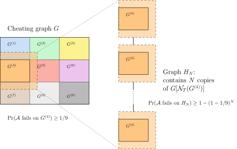
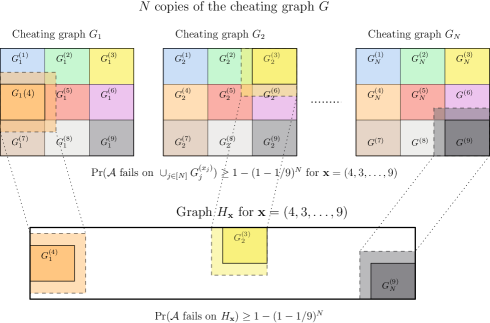
Figure 1: Construction for the $\operatorname{\mathsf{rand-LOCAL}}$ model. For any $T(n)$-round algorithm $\mathcal{A}$ solving the problem, there is an $i^{\star}\in[9]$ (in the figure, $i^{\star}=4$) such that $\Pr[\mathcal{A}\text{ fails in }G^{(i^{\star})}]\geq 1/9$. Then, $\Pr[\mathcal{A}\text{ fails on }H_{N}]\geq 1-(1-1/9)^{N}$ by independence, where $H_{N}$ is an admissible instance. As long as $\lvert V(H_{N})\rvert\leq n$, this gives the lower bound.

Figure 2: Construction for the $\operatorname{\mathsf{NS-LOCAL}}$ model. We start with $N$ copies $G_{1},\dots,G_{N}$ of $G$ and consider their disjoint union. We prove that, in this specific graph, there is already a combination of indices $\mathbf{x}=(x_{1},\dots,x_{N})\in[9]^{N}$ (in the figure, $\mathbf{x}=(4,3,\dots,9)$) for which $\Pr[\mathcal{A}\text{ fails on }\bigcup_{j\in[N]}G_{j}^{(x_{j})}]\geq 1-(1-1/9)^{N}$. Then, property (3) of Definition 2.1 ensures that we can construct an admissible instance $H_{\mathbf{x}}$ as shown in the figure, with $\lvert V(H_{\mathbf{x}})\rvert=n$. By the properties of the $\operatorname{\mathsf{NS-LOCAL}}$ model, since $H_{\mathbf{x}}$ and $\bigsqcup_{i\in[N]}G_{i}$ share the same local view around $\bigcup_{j\in[N]}G_{j}^{(x_{j})}$, $\mathcal{A}$ fails on $H_{\mathbf{x}}$ too with at least the same probability.

Figure 3: Illustration of the lower-bound argument based on the cheating graph $G$. For $n=\lvert V(G)\rvert\cdot N$, the problem is solvable in each $T(n)$-radius neighborhood of $G^{(i)}$, $i\in[9]$, but not on $G$.

If $k$ is not small enough (e.g., $k=w(1)$), the failing probability tends to $0$. In $\operatorname{\mathsf{rand-LOCAL}}$ we can amplify the failure probability as follows: Suppose $\mathcal{F}$ contains a graph $H_{N}$ of at most $n=\lvert V(G)\rvert\cdot N$ nodes that contains, as subgraphs, $N$ disjoint copies of the radius-$T(n)$ neighborhood of $G^{(i^{\star})}$ in $G$. This is always possible if $\mathcal{F}$ is the family of bipartite graphs. By independence, the failing probability of $\mathcal{A}$ over $H_{N}$ is at least $1-(1-1/k)^{N}$ (see Fig. 3). Hence, such an algorithm cannot exist. The property that $\mathcal{F}$ contains $H_{N}$ is reasonable for many natural problems (e.g., $c$-coloring $\chi$-chromatic graphs for all combinations of $c$ and $\chi$) where, given a graph for which the problem is solvable, one can connect disjoint copies of the graphs and obtain a solvable instance of the problem.

However, as we anticipated, in the $\operatorname{\mathsf{NS-LOCAL}}$ model some issues arise:

1. If two graphs $G$ and $H$ have different sizes, then even if they share two identical subgraphs $G^{\prime}$ and $H^{\prime}$ with isomorphic radius-$T$ neighborhoods, a non-signaling output distribution is not guaranteed to be identical over $G^{\prime}$ and $H^{\prime}$; this is due to the no-cloning principle [66, 25, 55].

2. If we look at the output distributions for two subsets of nodes $X$ and $Y$, then even if $X$ and $Y$ are far from each other, we cannot assume that the outputs of these subsets are independent.

Issue (i) puts some limits on the choice of the graph used to “fool” the algorithm, while issue (ii) makes it necessary to deal with possible dependencies among different parts of the input graph. Such issues are the reason why we require the cheating graph to satisfy property (3) in Definition 2.1.

To solve issue (i), we consider a graph that is the disjoint union of $N$ copies $G_{1},\dots,G_{n}$ of the cheating graph $G$: such graph has $\lvert V(G)\rvert\cdot N$ vertices, exactly the same as the graph of property (3) from Definition 2.1. Consider now any $\operatorname{\mathsf{NS-LOCAL}}$ algorithm $\mathcal{A}$ that $3$-colors bipartite graphs with locality $T$, and apply it to the graph $\sqcup_{i\in[N]}G_{i}$. Clearly, $\mathcal{A}$ will fail to solve the problem in each $G_{j}$ with probability 1. At this point, we cannot continue as before: while it is true that in each $G_{j}$ we can find an index $i^{\star}$ such that the probability of $\mathcal{A}$ failing in $G^{(i^{\star})}_{j}$ is at least $1/k$, we cannot use independence to increase the failing probability.

Property (3) ensures that, for a sufficiently large $N$, and for any sequence of indices $\mathbf{x}=(x_{1},\dots,x_{N})\in[k]^{N}$, there exists a graph $H_{\mathbf{x}}$ of size $\lvert V(G)\rvert\cdot N$ that contains an induced subgraph isomorphic to the disjoint union of the radius-$T$ neighborhoods of $G^{(x_{1})},\dots,G^{(x_{N})}$. However, correlations among these subgraphs of $H_{\mathbf{x}}$ might hold. To overcome this issue, we need to consider all possible sequences of subgraphs $G_{1}^{(x_{1})},\dots,G_{N}^{(x_{N})}$ at the same time, where $\mathbf{x}=(x_{1},\dots,x_{N})\in[k]^{N}$ (see Fig. 3). Fix a total order for the elements in $[k]^{N}$, and let its ordered elements be $\mathbf{x}_{1},\dots,\mathbf{x}_{k^{N}}$. Let $\mathcal{F}_{\mathbf{x}_{j}}$ be the event that $\mathcal{A}$ fails in $G^{(z_{i})}_{i}$, where $z_{i}$ is the $i$-th element of $\mathbf{x}_{j}$, for each $i=1,\dots,N$. Furthermore, for each index $\mathbf{x}\in[k]^{N}$, let $\mathcal{I}_{\mathbf{x}}$ be the set of all indices $\mathbf{y}\in[k]^{N}$ such that $\mathbf{y}$ and $\mathbf{x}$ share the same element at the $i$-th position, for some $i$, i.e., $\mathbf{x}(i)=\mathbf{y}(i)$. Notice that, for $\mathbf{x}=(x_{1},\dots,x_{N})$, $\cup_{\mathbf{y}\in\mathcal{I}_{\mathbf{x}}}\mathcal{F}_{\mathbf{y}}$ describes the event that there is an $i\in[N]$ such that $\mathcal{A}$ fails on $G_{i}^{(x_{i})}$.

We claim that there exists a $\mathbf{x}^{\star}\in[k]^{N}$ such that $\Pr\left[\cup_{\mathbf{y}\in\mathcal{I}_{\mathbf{x}^{\star}}}\mathcal{F}_{\mathbf{y}}\right]\geq 1-(1-1/k)^{N}$, implying that the dependencies behave “well enough”, hence solving issue (ii). We proceed by contradiction: we assume that, for all $\mathbf{x}\in[k]^{N}$, $\Pr\left[\cup_{\mathbf{y}\in\mathcal{I}_{\mathbf{x}}}\mathcal{F}_{\mathbf{y}}\right]<1-(1-1/k)^{N}$. While $\Pr\left[\cup_{\mathbf{x}\in[k]^{N}}{\mathcal{F}_{\mathbf{x}}}\right]=1$, the events in $\{\mathcal{F}_{\mathbf{x}}\}_{\mathbf{x}\in[k]^{N}}$ are not disjoint and the sum of their probability is not 1. To better deal with the math, we define $\mathcal{E}_{\mathbf{x}_{1}}=\mathcal{F}_{\mathbf{x}_{1}}$ and, recursively, we define $\mathcal{E}_{\mathbf{x}_{j}}=\mathcal{F}_{\mathbf{x}_{j}}\setminus(\cup_{i=1}^{j-1})\mathcal{E}_{\mathbf{x}_{i}}$. Clearly the events in $\{\mathcal{E}_{\mathbf{x}}\}_{\mathbf{x}\in[k]^{N}}$ are pairwise disjoint: furthermore, it holds that $\sum_{\mathbf{x}\in[k]^{N}}\Pr\left[\mathcal{E}_{\mathbf{x}}\right]=1$ as $\cup_{\mathbf{x}\in[k]^{N}}{\mathcal{E}_{\mathbf{x}}}=\cup_{\mathbf{x}\in[k]^{N}}{\mathcal{F}_{\mathbf{x}}}$. For each $\mathbf{x}\in[k]^{N}$, it trivially holds that

$$\sum_{\mathbf{y}\in\mathcal{I}_{\mathbf{x}}}\Pr\left[\mathcal{E}_{\mathbf{y}}\right]+\sum_{\mathbf{y}\in[k]^{N}\setminus\mathcal{I}_{\mathbf{x}}}\Pr\left[\mathcal{E}_{\mathbf{y}}\right]=1.$$

Moreover, for each $\mathbf{x}\in[k]^{N}$, we have $\Pr\left[\mathcal{E}_{\mathbf{x}}\right]\leq\Pr\left[\mathcal{F}_{\mathbf{x}}\right]$ as $\mathcal{E}_{\mathbf{x}}\subseteq\mathcal{F}_{\mathbf{x}}$, hence $\sum_{\mathbf{y}\in\mathcal{I}_{\mathbf{x}}}\Pr\left[\mathcal{E}_{\mathbf{y}}\right]<1-(1-1/k)^{N}$. Thus,

$$\sum_{\mathbf{y}\in[k]^{N}\setminus\mathcal{I}_{\mathbf{x}}}\Pr\left[\mathcal{E}_{\mathbf{y}}\right]>(1-1/k)^{N}.$$

It follows that

$$\sum_{\mathbf{x}\in[k]^{N}}\sum_{\mathbf{y}\in[k]^{N}\setminus\mathcal{I}_{\mathbf{x}}}\Pr\left[\mathcal{E}_{\mathbf{y}}\right]>k^{N}(1-1/k)^{N}=(k-1)^{N}.$$

Also, notice that for each $\mathbf{y}\in[k]^{N}$ the cardinality of the set $\left\{\mathbf{x}\in[k]^{N}\ \middle|\ \mathbf{y}\in[k]^{N}\setminus\mathcal{I}_{\mathbf{x}}\right\}$ is $(k-1)^{N}$. Hence,

$$\sum_{\mathbf{x}\in[k]^{N}}\sum_{y\in[k]^{N}\setminus\mathcal{I}_{\mathbf{x}}}\Pr\left[\mathcal{E}_{\mathbf{y}}\right] =\sum_{\mathbf{y}\in[k]^{N}}\sum_{\begin{subarray}{c}\mathbf{x}\in[k]^{N}:\\ \mathbf{y}\in[k]^{N}\setminus\mathcal{I}_{\mathbf{x}}\end{subarray}}\Pr\left[\mathcal{E}_{\mathbf{y}}\right]=(k-1)^{N}\sum_{\mathbf{y}\in[k]^{N}}\Pr\left[\mathcal{E}_{\mathbf{y}}\right]=(k-1)^{N},$$

reaching a contradiction. Thus, there exists an $\mathbf{x}^{\star}\in[k]^{N}$ such that $\Pr\left[\cup_{\mathbf{y}\in\mathcal{I}_{\mathbf{x}^{\star}}}\mathcal{F}_{\mathbf{y}}\right]\geq 1-(1-1/k)^{N}.$ Property (3) of Definition 2.1 ensures that there is a graph $H_{\mathbf{x}^{\star}}\in\mathcal{F}$ of $n$ nodes such that $H_{\mathbf{x}^{\star}}$ contains, as induced subgraph, $\cup_{i\in[N]}G_{i}^{(\mathbf{x}^{\star}_{i})}$, and $H_{\mathbf{x}^{\star}}$ and $\sqcup_{i\in[N]}G_{i}$ share the same radius-$T(n)$ neighborhood around $\cup_{i\in[N]}G_{i}^{(\mathbf{x}^{\star}_{i})}$. By the property of the $\operatorname{\mathsf{NS-LOCAL}}$ model, we get that the failing probability of $\mathcal{A}$ on $H_{\mathbf{x}^{\star}}$ is at least $1-(1-1/k)^{N}$.

3 Preliminaries

We consider the set $\mathbb{N}$ of natural numbers to start with 0. We also define $\mathbb{N}_{+}=\mathbb{N}\setminus\{0\}$. For any positive integer $n\in\mathbb{N}_{+}$, we denote the set $\{1,\dots,n\}$ by $[n]$.

Graphs.

All graphs in this paper are simple graphs without self-loops. Let $G=(V,E)$ be a simple graph with $n\in\mathbb{N}$ nodes. If the set of nodes and the set of edges are not specified, we refer to them by $V(G)$ and $E(G)$, respectively. For any edge $e=\{u,v\}\in E(G)$, we also write $e=uv=vu$.

If $G$ is a subgraph of $H$, we write $G\subseteq H$. For any subset of nodes $A\subseteq V$, we denote by $G[A]$ the subgraph induced by the nodes in $A$. For any nodes $u,v\in V$, $\operatorname{dist}_{G}(u,v)$ denotes the distance between $u$ and $v$ in $G$ (i.e., the number of edges of any shortest path between $u$ and $v$ in $G$); if $u$ and $v$ are disconnected, then $\operatorname{dist}_{G}(u,v)=+\infty$. If $G$ is clear from the context, we may also simply write $\operatorname{dist}(u,v)=\operatorname{dist}_{G}(u,v)$. For $T\in[n]$, the $T$-neighborhood of a node $u\in V$ is the set $\mathcal{N}_{T}(u)=\left\{v\in V\ \middle|\ \operatorname{dist}(u,v)\leq T\right\}$. The $T$-neighborhood of a subset $A\subseteq V$ is the set $\mathcal{N}_{T}(A)=\left\{v\in V\ \middle|\ \exists u\in A:\operatorname{dist}(u,v)\leq T\right\}$. Similarly, the $T$-neighborhood of a subgraph $H\subseteq G$ is the set $\mathcal{N}_{T}(H)=\left\{v\in V(G)\ \middle|\ \exists u\in V(H):\operatorname{dist}_{G}(u,v)\leq T\right\}$.

For $c\in\mathbb{N}$, a $c$-coloring of a graph $G$ is a map $\varphi\colon V(G)\to[c]$. The coloring $\varphi$ is said to be proper if we have $\varphi(u)\neq\varphi(v)$ for every $uv\in E$. If, for some $\chi\in\mathbb{N}$, there exists a proper $\chi$-coloring for $G$ and $\chi$ is minimal with this property, then $G$ is said to be $\chi$-chromatic; we also say that the chromatic number of $G$, denoted by $\mathcal{X}(G)$, is $\chi$. In the $c$-coloring problem, the input is a graph $G$, and the task is to find a proper $c$-coloring of $G$.

The $\operatorname{\mathsf{LOCAL}}$ model.

The $\operatorname{\mathsf{LOCAL}}$ model is a distributed system consisting of a set of $\lvert V\rvert=n$ processors (or nodes) that operates in a sequence of synchronous rounds. In each round the processors may perform unbounded computations on their respective local state variables and subsequently exchange of messages of arbitrary size along the links given by the underlying input graph. Nodes identify their neighbors by using integer labels assigned successively to communication ports. (This assignment may be done adversarially.) Barring their degree, all nodes are identical and operate according to the same local computation procedures. Initially all local state variables have the same value for all processors; the sole exception is a distinguished local variable $x(v)$ of each processor $v$ that encodes input data.

Let $c\geq 1$ be a constant, and let $\Sigma_{\text{in}}$ be a set of input labels. The input of a problem is defined in the form of a labeled graph $(G,x)$ where $G=(V,E)$ is the system graph, $V$ is the set of processors (hence it is specified as part of the input), and $x\colon V\to[n^{c}]\times\Sigma_{\text{in}}$ is an assignment of a unique identifier $\text{id}(v)\in[n^{c}]$ and of an input label $\lambda_{\text{in}}(v)\in\Sigma_{\text{in}}$ to each processor $v$. The output of the algorithm is given in the form of a vector of local output labels $\lambda_{\text{out}}\colon V\to\Sigma_{\text{out}}$, and the algorithm is assumed to terminate once all labels $\lambda_{\text{out}}(v)$ are definitely fixed. We assume that nodes and their links are fault-free. The local computation procedures may be randomized by giving each processor access to its own set of random variables; in this case, we are in the randomized $\operatorname{\mathsf{LOCAL}}$ ($\operatorname{\mathsf{rand-LOCAL}}$) model as opposed to deterministic $\operatorname{\mathsf{LOCAL}}$ ($\operatorname{\mathsf{det-LOCAL}}$).

The running time of an algorithm is the number of synchronous rounds required by all nodes to produce output labels. If an algorithm running time is $T$, we also say that the algorithm has locality $T$. Notice that $T$ can be a function of the size of the input graph.

We say that the $c$-coloring problem over some graph family $\mathcal{F}$ has complexity $T$ in the $\operatorname{\mathsf{det-LOCAL}}$ model if there exists a $\operatorname{\mathsf{det-LOCAL}}$ algorithm solving the problem in time $T$ for all input graphs $G\in\mathcal{F}$, but no $\operatorname{\mathsf{det-LOCAL}}$ algorithm solves the problem in time $T-1$ (where $T$ can be a function of the input graph size) for all input graphs $G\in\mathcal{F}$. The complexity in the $\operatorname{\mathsf{rand-LOCAL}}$ model is defined similarly.

4 New classical graph coloring algorithms

In this section we prove the existence of algorithms in $\operatorname{\mathsf{det-LOCAL}}$ and $\operatorname{\mathsf{rand-LOCAL}}$ that almost match the $\operatorname{\mathsf{NS-LOCAL}}$ lower bound. We recall here the precise statement for the reader’s convenience.

See 1.1

Notice that, if we plug in the same parameters (with $c=\alpha(\chi-1)+1$) in Theorem 1.3 with an appropriate choice of constant $\varepsilon$, we get that $\alpha=\left\lfloor\frac{c-1}{\chi-1}\right\rfloor$, implying a lower bound of $\Omega\!\left(n^{1/\alpha}/\chi^{1+1/\alpha}\right)$ for the problem. Therefore, for constant $\chi$ and $\alpha$, our algorithms give a perfect trade-off between quality of approximation and time complexity up to logarithmic factors.

Fast coloring from fast network decomposition.

Our algorithm follows an approach similar to that of [13], which in turn is based on network decompositions.

Definition 4.1 (Network decomposition).

An $(\alpha,d)$-network decomposition of a graph $G$ is a partition $V(G)=C_{1}\cup\dots\cup C_{k}$ along with a map $\mu\colon\{C_{1},\dots,C_{k}\}\to[\alpha]$ meeting the following conditions:

• The clusters $C_{i}$ are pairwise disjoint (i.e., $C_{i}\cap C_{j}=\varnothing$ unless $i=j$).

• For every $i$, the (weak) diameter $\max_{u,v\in C_{i}}\operatorname{dist}_{G}(u,v)$ of $C_{i}$ is at most $d$.

• The supergraph $S=S(G)$ with node set $V(S)=\{C_{1},\dots,C_{k}\}$ and edge set $E(S)=\{\{C_{i},C_{j}\}\mid\exists u\in C_{i},v\in C_{j}:\{u,v\}\in E(G)\}$ that is obtained by contracting each $C_{i}$ is $\alpha$-colorable.

• $\mu$ is an $\alpha$-coloring of $S$.

In addition, the coloring $\mu$ is presented explicitly to the nodes of $G$; that is, every node $v\in C_{i}$ knows the cluster color $\mu(C_{i})$ of its respective cluster $C_{i}$.

We recall the algorithm of [13]. Suppose we are given an $(\alpha,d(n))$-network decomposition $\mathcal{D}$. We iterate sequentially through the $\alpha$ cluster colors of $\mathcal{D}$. For each cluster color $a$ and each cluster $C$ having the cluster color $\mu(C)=a$, collect the entire topology of $C$ in some arbitrary node $v\in C$ (chosen by, e.g., leader election). The node $v$ then computes a perfect coloring $\pi$ for the nodes of $C$ that uses at most $\chi$ colors and then broadcasts to each node $u\in C$ its color $\pi(u)$. Clearly in the $\operatorname{\mathsf{LOCAL}}$ model each iteration takes at most diameter of $C_{i}$ many rounds, so at most $\mathcal{O}\!\left(d(n)\right)$ rounds. With a clever implementation, this process can also be sped up by doing all the iterations in parallel. We will see this in the later sections.

In order for this strategy to work, we must ensure that neighboring clusters use distinct sets of colors; otherwise, the colorings of the nodes of neighboring clusters may not match. To deal with this, we have clusters of different cluster colors use completely different sets of colors for the nodes, which we will refer to as color palettes. More precisely, each cluster $C$ of cluster color $\mu(C)=a$ may only use colors from the palette $p_{a}=\{(a,b)\mid b\in\mathbb{N}_{+}\}$. Since there are $\alpha$ many colors for the clusters, (assuming each cluster is colored using at most $\chi$ colors) this then gives a coloring of $G$ with $\alpha\chi$ colors. As we color each cluster by gathering its entire structure in a single node, knowledge of $\chi$ is not needed in order to use the optimal number of colors for each cluster.

The “hiding trick”.

We show how to optimize the above strategy using what we call a “hiding trick”. We add one special hidden color $-1$ in common to all color palettes $p_{a}$ and that is guaranteed to appear only in the “inside” of the clusters; that is, if a node $v$ in some cluster $C$ has a neighbor that is not in $C$, then $v$ is guaranteed to not be colored $-1$. This ensures the colorings produced by two neighboring clusters are still compatible since the only color shared by their palettes is the hidden color $-1$, which is only present in the “insides” of the clusters. Since the palettes now share exactly one color, this allows us to save $\alpha-1$ colors in total. Surprisingly enough, this small modification is enough to attain the minimum number of colors possible, that is, $\alpha(\chi-1)+1$ colors (as per our lower bound from Theorem 1.3).

Fast decomposition from fast clustering.

The specific complexity of the resulting algorithm depends on value $d(n)$ of the underlying decomposition $\mathcal{D}$. We show how to obtain a decomposition with $d(n)=\tilde{\mathcal{O}}\!\left(n^{1/\alpha}\right)$ in $\mathcal{O}\!\left(d(n)\right)$ time. To do so, we show how to efficiently turn any existing clustering algorithm into a network decomposition algorithm. The difference between the two is that the former only needs to group a subset of nodes in the graph, whereas the latter must partition the entire graph.

Definition 4.2 ($(\lambda,d)$-clustering).

Given a graph $G$, a $(\lambda,d)$-clustering is a partition $V(G)=D\cup S_{1}\cup\dots\cup S_{k}$ meeting the following conditions:

• $S_{1},\dots,S_{k}$ are mutually non-adjacent; that is, the distance between any two nodes $u\in S_{i}$ and $v\in S_{j}$ where $i\neq j$ is at least 2.

• For every $i$, the (weak) diameter $\max_{u,v\in S_{i}}\operatorname{dist}_{G}(u,v)$ of $S_{i}$ is at most $d$.

• $D$ contains at most $\lambda\lvert V(G)\rvert$ vertices.

Our conversion from a clustering algorithm into a network decomposition one is by a bootstrapping procedure: if the clustering algorithm is guaranteed to cluster at least half of the nodes in $G$, then we can apply it again and again until only an $\varepsilon$ fraction of nodes remains unclustered, where $\varepsilon$ is a parameter of our choosing. For an appropriate choice of $\varepsilon$, the fraction of nodes that remains is sufficiently small that we can directly gather the remaining nodes into their own cluster (simply by grouping every remaining connected component of the graph).

Organization.

In Section 4.1 we show how to obtain a fast coloring algorithm given the underlying network decomposition $\mathcal{D}$. In Section 4.2 we then show how to obtain such a decomposition following the two-step approach described above: first we show our bootstrapping result for clustering algorithms in Section 4.2.1 and then how this implies a network decomposition algorithm in Section 4.2.2. Plugging in the state-of-the-art for clustering algorithms, we then obtain Theorem 1.1.

4.1 The hiding trick

The main result of this section is the following, which is a coloring algorithm based on our so-called hiding trick (see also Lemma 4.4 below). The algorithm presupposes the existence of a network decomposition algorithm, which we show how to obtain in Section 4.2.

Theorem 4.3.

Fix some parameter $\alpha\in\mathbb{N}$ and suppose there is an $(\alpha,d(n))$-network decomposition algorithm $\mathcal{B}$ for $\operatorname{\mathsf{det-LOCAL}}$ or $\operatorname{\mathsf{rand-LOCAL}}$ that runs in time $d(n)$. Then there is an algorithm $\mathcal{A}$ that $(\alpha(\chi-1)+1)$-colors any $\chi$-chromatic graph $G$ with $n$ nodes in $O(d(n))$ time. Moreover, $\mathcal{A}$ works in $\operatorname{\mathsf{det-LOCAL}}$ or $\operatorname{\mathsf{rand-LOCAL}}$, depending on which model $\mathcal{B}$ runs in. In addition, if $\mathcal{B}$ is randomized (i.e., it is a $\operatorname{\mathsf{rand-LOCAL}}$ algorithm) and succeeds with probability $1-1/\poly(n)$, then so does $\mathcal{A}$ succeed with probability $1-1/\poly(n)$.

The core idea of our algorithm is the following constructive lemma. It shows that, in any graph $G$, it is always possible to color a subset $A$ of nodes in a way that “hides” one designated hidden color $-1$. To color $A$ in this manner, it may be necessary to fix the color of some nodes in $N(A)$ as well.

Lemma 4.4 (Hiding Lemma).

Let $G=(V,E)$ be a graph, and let $\chi$ be the chromatic number of $G$. For any subset $A\subseteq V$, there exists $A\subseteq A^{\prime}\subseteq(A\cup N(A))$ and a proper coloring $\varphi\colon A^{\prime}\rightarrow[\chi-1]\cup\{-1\}$ of $A^{\prime}$ such that $A$ is completely colored and, for any node $v\in V\setminus A^{\prime}$, $v$ is not adjacent to a node with color $-1$.

Proof.

Since $G$ is $\chi$-colorable, there exists a $\chi$-coloring $\psi$ of $A\cup N(A)$. We uncolor some of the nodes of $N(A)$ such that none of the uncolored nodes has a neighbor with color $-1$. Formally, let

$$A^{\prime}=(A\cup N(A))\setminus\{u\in N(A)\mid\psi(u)=-1\}$$

and $\varphi=\psi{\restriction_{A^{\prime}}}$ (i.e., the restriction of $\psi$ to $A^{\prime}$). Since we only uncolor nodes in $N(A)$ and $\psi$ is a proper $\chi$-coloring of $A\cup N(A)$, $\varphi$ is certainly a proper coloring of $A^{\prime}\subseteq(A\cup N(A))$. We now argue that $v\in V\setminus A^{\prime}$ has no neighbor that is colored $-1$ by $\varphi$. Since $A\subseteq A^{\prime}$, we must consider only the following two cases:

$v\in N(A)$.

Since $v$ is not in $A^{\prime}$ but still in $N(A)$, $\psi(v)=-1$. Hence, since $\psi$ is a proper coloring, every node in $N(v)$ colored by $\psi$ has a color that is different from $-1$. Since $\varphi$ is a restriction of $\psi$, the same holds for any node in $N(v)$ colored by $\varphi$.

$v\notin A\cup N(A)$.

Then $v$ is only adjacent to nodes in $N(A)$. Since no node in $N(A)$ is colored $-1$ by $\varphi$ by definition, clearly $v$ has no neighbor colored $-1$ by $\varphi$. ∎

Note that Lemma 4.4 (in its current form) cannot be immediately applied to a decomposition of $G$ to produce colorings for the clusters of $G$. The reason for that is the following: Consider two clusters $C$ and $C^{\prime}$ that are assigned the same cluster color $a$ by the network decomposition. (In particular, this means $C$ and $C^{\prime}$ are not adjacent.) Recall that we will color the nodes of $C$ and $C^{\prime}$ using the same color palette. However, if we color them such as in Lemma 4.4, then we are potentially also coloring nodes in $N(C)$ and $N(C^{\prime})$ and, for all we know, the intersection $N(C)\cap N(C^{\prime})$ may not be empty. Hence we cannot simply use the same color palette in both clusters, as this could potentially lead to an invalid coloring.

Therefore, we would like that not only $C$ and $C^{\prime}$ but also $N(C)$ and $N(C^{\prime})$ are not adjacent. Equivalently, we wish for the distance between $C$ and $C^{\prime}$ to be at least $4$. We can indirectly guarantee this by using an $(\alpha,d(n))$-network decomposition $\mathcal{D}$ of $G^{3}$ instead of $G$. This is because being not adjacent in $G^{3}$ immediately implies a distance of at least $4$ in $G$. Asymptotically speaking, this does not incur any additional cost (compared to computing a decomposition of $G$) since, for any $k$, we can simulate each round of communication in $G^{k}$ by using $k$ rounds of communication in $G$.

We now present Algorithm 1, which, given a $\chi$-chromatic graph $G$ and an $(\alpha,d(n))$-network decomposition $\mathcal{D}$ of $G^{3}$, colors $G$ using $\alpha(\chi-1)+1$ colors. By proving the correctness of Algorithm 1 we then obtain Theorem 4.3.

Algorithm 1 Coloring a decomposition

1:$G=(V,E)$, $(\alpha,d(n))$-network decomposition $\mathcal{D}$ of $G^{3}$

2:for each cluster $C_{i}$ in parallel do

3:     Elect a leader node $\mathtt{leader}_{i}$ of $C_{i}$

4:     Collect the entire topology of $C_{i}\cup N(C_{i})$ in $\mathtt{leader}_{i}$

5:     $a\leftarrow\text{the cluster color assigned to $C_{i}$ by $\mathcal{D}$}$

6:     $p_{a}\leftarrow\{(a,b)\mid b\in\mathbb{N}\}\cup\{-1\}$

7:     if $a=\alpha$ then

8:         $\mathtt{leader}_{i}$ computes a minimal coloring $\varphi_{i}\colon C_{i}\to p_{a}$ of $C_{i}$

9:         $\mathtt{leader}_{i}$ broadcasts $\varphi_{i}$ to all nodes in $C_{i}$

10:     else

11:         $\mathtt{leader}_{i}$ computes a minimal node coloring $\varphi_{i}\colon C_{i}^{\prime}\to p_{a}$ of some $C_{i}^{\prime}\subseteq C_{i}\cup N(C_{i})$ according to Lemma 4.4

12:         $\mathtt{leader}_{i}$ broadcasts $\varphi_{i}$ to all nodes in $C_{i}\cup N(C_{i})$

13:     end if

14:end for

15:for each node $u$ in parallel do

16:     $\Phi_{u}\leftarrow\text{the set of all colors assigned to $u$ by the $\varphi_{i}$}$

17:     if $\Phi_{u}=\{-1\}$ then

18:         Color $u$ with the color $-1$

19:     else

20:         Color $u$ with an arbitrary color from $\Phi_{u}\setminus\{-1\}$

21:     end if

22:end for

23:Each node outputs its own color

Let us give a brief high-level description of Algorithm 1. Each cluster $C_{i}$ acts independently and based on the cluster color $a$ that is assigned to it by the decomposition $\mathcal{D}$. First, the entire topology of $C_{i}\cup N(C_{i})$ is gathered in some leader node $\mathtt{leader}_{i}$. Next $\mathtt{leader}_{i}$ brute-forces an optimal coloring $\varphi_{i}$ of its respective cluster $C_{i}$ using a color palette $p_{a}$ that depends on $a$. (Without restriction we use only the smallest elements of $p_{a}$ (according to the natural ordering of $p_{a}$) in $\varphi_{i}$. This enables the nodes to choose correct colors even without knowledge of $\chi$.) If $a=\alpha$, $\varphi_{i}$ is simply a $\chi$-coloring of $C_{i}$ whose existence is guaranteed by the $\chi$-chromaticness of $G$. Otherwise (i.e., if $a<\alpha$), $\mathtt{leader}_{i}$ instead computes a coloring $\varphi_{i}$ of $C_{i}^{\prime}\subseteq C_{i}\cup N(C_{i})$ according to Lemma 4.4. Each coloring $\varphi_{i}$ is broadcasted to all nodes that may have been assigned a color by $\varphi_{i}$. The nodes that were assigned multiple colors (i.e., potentially those at the border of two distinct clusters) then simply choose one of them arbitrarily.

Lemma 4.5.

Algorithm 1 computes a valid coloring of $G$ using no more than $\alpha(\chi-1)+1$ colors.

Proof.

First we argue that no more than $\alpha(\chi-1)+1$ colors are used in total. For a cluster color $a\in[\alpha]$, let

$$p_{a}^{\prime}=\{\varphi_{i}(v)\mid\exists i:\mu(C_{i})=a\land v\in C_{i}\}\subseteq p_{a}$$

be the set of colors actually used by the nodes to color clusters with the color $a$. By the $\chi$-chromaticness of $G$, every minimal coloring of any induced subgraph of $G$ uses at most $\chi$ colors, so we have $\lvert p_{a}^{\prime}\rvert\leq\chi$. Since the intersection of two palettes $p_{a}$ and $p_{b}$ is exactly $\{-1\}$ for $a\neq b$, we use

$$\left\lvert\bigcup_{a=1}^{\alpha}p_{a}^{\prime}\right\rvert=\left\lvert\{-1\}\right\rvert+\sum_{a=1}^{\alpha}\left\lvert p_{a}^{\prime}\setminus\{-1\}\right\rvert\leq\alpha(\chi-1)+1$$

colors in total, as claimed.

To show that the color is proper, first observe that, based on Lemma 4.4, no node in $N(C_{i})$ is assigned $-1$ by $\varphi_{i}$; as a result, if a node $v$ is assigned the color $-1$ by $\varphi_{i}$, then necessarily $v\in C_{i}$. Consider any two adjacent nodes $v$ and $v^{\prime}$ and recall that both of them choose the largest color among any of the colors they were assigned. For the sake of contradiction, suppose that both nodes pick the same color $x$. Consider the following two cases:

$x\neq-1$.

Since the intersection of any two color palettes is $\{-1\}$, this implies that $v$ and $v^{\prime}$ were assigned colors from the same color palette $p_{a}$. Since the $\varphi_{i}$ are all valid colorings, the colors of $v$ and $v^{\prime}$ come from different coloring functions $\varphi_{i}$ and $\varphi_{i^{\prime}}$, respectively. However, since $\varphi_{i}$ and $\varphi_{i^{\prime}}$ use the same color palette, the respective clusters $C_{i}$ and $C_{i^{\prime}}$ are assigned the same cluster color by $\mathcal{D}$. This means that $C_{i}$ and $C_{i^{\prime}}$ are not adjacent in $G^{3}$ and, in turn, the distance between nodes in $N(C_{i})$ and $N(C_{i^{\prime}})$ is at least $2$, which immediately contradicts $v$ and $v^{\prime}$ being adjacent.

$x=-1$.

This means that both of the nodes are assigned their color by the coloring of their respective cluster. Let $i$ and $i^{\prime}$ be the numbers of the clusters of $v$ and $v^{\prime}$, respectively. If $i=i^{\prime}$, then both $v$ and $v^{\prime}$ pick their colors according to $\varphi_{i}=\varphi_{i^{\prime}}$, which contradicts $\varphi_{i}$ being a proper coloring. Hence let $i\neq i^{\prime}$. We have then that $C_{i}$ and $C_{i^{\prime}}$ are adjacent clusters and, since they are distinct, without restriction we have $i\neq\alpha$. Since $v^{\prime}\in N(C_{i})$ and the color of both $v$ and $v^{\prime}$ is $-1$, Lemma 4.4 implies that $v^{\prime}$ is in the domain of $\varphi_{i}$ (as otherwise it would be adjacent to $v$, which has the color $-1$). Now since $\varphi_{i}(v)=-1$, we know that $\varphi_{i}(v^{\prime})>-1$, which means that the color of $v^{\prime}$ cannot be $-1$. ∎

Note that, in the proof above, we simply showed that no more than $c=\alpha(\chi-1)+1$ colors are used, but there is still a minor technicality to be dealt with since the colors do not come from the set $[c]$ as the definition of $c$-coloring demands (but rather either the color is $-1$ or a pair $(a,b)$). A straightforward way of resolving this is, for instance, remapping $-1$ to $1$ and every pair $(a,b)\in p_{a}$ to $\alpha(b-1)+a+1$. (Note this gives a bijection between $\{-1\}\cup\bigcup_{a\in[\alpha]}p_{a}$ and $\mathbb{N}_{+}$.) Since we use only the smallest elements of the palette $p_{a}$ in each respective coloring $\varphi_{i}$, we know that any $(a,b)\in p_{a}^{\prime}$ must be such that $b\leq\chi-1$. Hence the largest color used is $\alpha(\chi-2)+\alpha+1=c$ (corresponding to $(\alpha,\chi-1)\in p_{\alpha}$).

Lemma 4.6.

Given the $(\alpha,d(n))$-network decomposition $\mathcal{D}$, Algorithm 1 can be run distributedly in $\mathcal{O}\!\left(d(n)\right)$ rounds in the $\operatorname{\mathsf{det-LOCAL}}$ model.

Proof.

The only lines in the algorithm that require communication are 3, 4 and 12. Since our clusters have diameter at most $d(n)$, 3 requires only $\mathcal{O}\!\left(d(n)\right)$ rounds of communication. The other two trivially take only $d(n)+1$ rounds since the message size in the $\operatorname{\mathsf{det-LOCAL}}$ model is unbounded and also any node in $N(C_{i})$ has distance at most $d(n)+1$ to its respective $\mathtt{leader}_{i}$. All other steps in the algorithm are local computations that do not incur any cost in the $\operatorname{\mathsf{det-LOCAL}}$ model. ∎

Together, Lemmas 4.5 and 4.6 prove Algorithm 1 satisfies the requirements of Theorem 4.3, thus concluding its proof.

4.2 Fast network decomposition

Given any clustering algorithm, we can obtain a network decomposition algorithm as follows.

Theorem 4.7.

Let $f,g\colon\mathbb{N}\to\mathbb{N}$ be arbitrary functions and suppose there is an $\mathcal{O}\!\left(f(n)\right)$-round distributed $(1/2,g(n))$-clustering algorithm named cluster for $\operatorname{\mathsf{det-LOCAL}}$ or $\operatorname{\mathsf{rand-LOCAL}}$. There is an algorithm $\mathcal{A}$ that, given a graph $G=(V,E)$ and any $\alpha\in\mathbb{N}_{+}$, computes an $(\alpha,\mathcal{O}(n^{1/\alpha}g(n)))$-network decomposition of $G$ in

$$d(n)=\mathcal{O}\!\left(\left(\frac{n}{g(n)}\right)^{1/\alpha}\left(f(n)+g(n)\right)\log\frac{n}{g(n)}\right)$$

rounds. The algorithm $\mathcal{A}$ works in $\operatorname{\mathsf{det-LOCAL}}$ or $\operatorname{\mathsf{rand-LOCAL}}$, depending on which model cluster itself is based on. In addition, if cluster is randomized and succeeds with probability $1-1/\poly(n)$, then $\mathcal{A}$ also succeeds with probability $1-1/\poly(n)$.

We mention two state-of-the-art clustering algorithms that can be plugged into Theorem 4.7, one for the $\operatorname{\mathsf{det-LOCAL}}$ model and one for the $\operatorname{\mathsf{rand-LOCAL}}$ model. For the $\operatorname{\mathsf{det-LOCAL}}$ model we use the clustering algorithm from [34]. In fact this algorithm actually works even in the more restricted $\operatorname{\mathsf{CONGEST}}$ model, where each node can only send $O(\log n)$-bit messages each round.

Theorem 4.8 ([34]).

There exists an algorithm that computes a $(1/2,\mathcal{O}\!\left(\log n\cdot\log\log\log n\right))$-clustering in $\operatorname{\mathsf{det-CONGEST}}$ in $\tilde{\mathcal{O}}\!\left(\log^{2}n\right)$ rounds.

Plugging in this algorithm in Theorem 4.7, we obtain the first item of Theorem 1.1. For the $\operatorname{\mathsf{rand-LOCAL}}$ model (i.e., the second item of Theorem 1.1), we use the following.

Theorem 4.9 ([23]).

There exists an algorithm that computes a $(1/2,\mathcal{O}(\log n))$-clustering in the $\operatorname{\mathsf{rand-LOCAL}}$ model in $\mathcal{O}\!\left(\log n\right)$ rounds with probability $1-1/\poly(n)$.

There are two steps to the proof of Theorem 4.7. In Section 4.2.1 we show a bootstrapping result where we use the $(1/2,g(n))$-clustering algorithm cluster to obtain a $(\varepsilon,\mathcal{O}(g(n)/\varepsilon))$-clustering algorithm for any $\varepsilon$ of our choosing. Plugging in an adequate value for $\varepsilon$, in Section 4.2.2 we then obtain the network decomposition algorithm of Theorem 4.7.

4.2.1 Fast clustering

Next we show our bootstrapping procedure, with which we can reduce a $1/2$ fraction of unclustered nodes to any $\varepsilon$ of our choosing. The price to pay is only a multiplicative $\mathcal{O}\!\left(1/\varepsilon\right)$ factor in the diameter of the clusters and a multiplicative $\mathcal{O}\!\left(\varepsilon^{-1}\log(1/\varepsilon)\right)$ factor in the running time. Formally, what we achieve is the following:

Theorem 4.10.

Let cluster be as in Theorem 4.7. For any $0<\varepsilon\leq 1$, there is an algorithm $\varepsilon$-cluster that computes an $(\varepsilon,\mathcal{O}\!\left(g(n)/\varepsilon\right))$-clustering in

$$\mathcal{O}\!\left(\frac{(f(n)+g(n))\log(1/\varepsilon)}{\varepsilon}\right)$$

rounds. The algorithm $\varepsilon$-cluster can be implemented in the same distributed model as cluster and its runtime is dominated by $2\log(1/\varepsilon)$ invocations of cluster. In addition, if cluster is randomized (i.e., it works in $\operatorname{\mathsf{rand-LOCAL}}$) and succeeds with probability $1-1/\poly(n)$, then $\varepsilon$-cluster also succeeds with probability $1-1/\poly(n)$.

We first describe the algorithm (Algorithm 2) and then prove it satisfies the properties of Theorem 4.10. Note that, in the description of Algorithm 2 in all three Lines 8,9 and 10 the neighborhoods are always taken with respect to $G$.

Algorithm 2 Bootstrapping cluster

1:$G=(V,E),0<\varepsilon\leq 1$

2:Clustering algorithm cluster as in Theorem 4.10

3:$R\leftarrow 4/\varepsilon$

4:$\mathcal{C^{\prime}}\leftarrow\text{empty clustering}$

5:for $2\log(1/\varepsilon)$ times do

6:     Run cluster on $G^{2R+1}$, producing a clustering $\mathcal{C}$

7:     for each cluster $C\in\mathcal{C}$ in parallel do

8:         Find $j^{*}\in[R]$ such that $\lvert\mathcal{N}_{j^{*}}(C)\setminus\mathcal{N}_{j^{*}-1}(C)\rvert$ is minimized

9:         Mark all nodes in $\mathcal{N}_{j^{*}}(C)\setminus\mathcal{N}_{j^{*}-1}(C)$ for deletion

10:         Add $\mathcal{N}_{j^{*}-1}(C)$ as a cluster to $\mathcal{C}^{\prime}$

11:     end for

12:     Let $U$ be the set of nodes not marked for deletion or that did not join a cluster of $\mathcal{C^{\prime}}$

13:     $G\leftarrow G[U]$

14:end for

15:Each node outputs whether it is part of a cluster of $\mathcal{C}^{\prime}$ or not

At a high level, Algorithm 2 works in multiple iterations, in each of which we first invoke cluster. For each new cluster $C$ that is computed, we delete some boundary around this cluster and separate it from the rest of the graph. We then add $C$ to our final clustering. Since cluster clusters at least half of the nodes, the size of our graph is halved in each iteration; hence after $\mathcal{O}\!\left(2\log 1/\varepsilon\right)$ iterations we are left with only an $\varepsilon$ fraction of nodes.

The main challenge lies in the choice of the boundaries and preventing too many nodes from being deleted. To solve this we appeal to the computational power of the $\operatorname{\mathsf{LOCAL}}$ model: For each cluster $C$, we inspect the $(4/\varepsilon)$-hop neighborhood of $C$ and find $j^{*}$ such that the number of nodes at distance exactly $j^{*}$ from $C$ (i.e., $\lvert\mathcal{N}_{j^{*}}(C)\setminus\mathcal{N}_{j^{*}-1}(C)\rvert$) is minimized. As we will show, there is always a choice of $j^{*}$ such that the number of nodes we delete is not too large.

We now turn to showing that Algorithm 2 satisfies the properties in Theorem 4.10. To give an overview, we need to prove the following:

1. The clusters created have diameter $\mathcal{O}\!\left(g(n)/\varepsilon\right)$ and are non-adjacent (Lemma 4.11).

2. At least a $1-\varepsilon$ fraction of the nodes get clustered (Lemma 4.12).

3. Algorithm 2 runs in $O((f(n)+g(n))\cdot\varepsilon^{-1}\log(1/\varepsilon))$ rounds (Lemma 4.13).

4. If cluster is randomized and has success probability $1-1/\poly(n)$, then Algorithm 2 also succeeds with probability $1-1/\poly(n)$ (Lemma 4.14).

We address these claims now one by one.

Lemma 4.11.

The clusters created by Algorithm 2 have diameter $\mathcal{O}\!\left(g(n)/\varepsilon\right)$ and are non-adjacent.

Proof.

We start by analyzing a single iteration of the for loop on 5 and show that a cluster with diameter $\mathcal{O}\!\left(g(n)/\varepsilon\right)$ is created. Afterwards we prove that, once a good cluster is created, it is preserved by later iterations.

Algorithm 2 runs the algorithm cluster of Theorem 4.8 on the power graph $G^{2R+1}$. Let $C_{i},C_{j}$ be two clusters created by cluster. For any nodes $u\in C_{i}$ and $v\in C_{j}$ with $i\neq j$, we have $\operatorname{dist}_{G^{\prime}}(u,v)\geq 2$, which implies $\operatorname{dist}_{G}(u,v)\geq 2R+2$. Let $S_{i}\in\mathcal{S}$ and $S_{j}\in\mathcal{S}$ be the clusters that are fixed by 10 in the iterations of $C_{i}$ and $C_{j}$, respectively. We observe that $S_{i}$ (resp., $S_{j}$) only contains nodes at distance at most $R-1$ from $C_{i}$ (resp., $C_{j}$). Hence it follows that, for any $u^{\prime}\in S_{i}$ and $v^{\prime}\in S_{j}$, we have $\operatorname{dist}_{G}(u^{\prime},v^{\prime})>2R+2-2(R-1)\geq 4$.

In addition, cluster guarantees that the diameter of the clusters is at most $g(n)$ in $G^{2R+1}$. Therefore, for $u,v\in C_{i}$,

$$\operatorname{dist}_{G}(u,v)\leq(2R+1)\operatorname{dist}_{G^{\prime}}(u,v)\leq(2R+1)g(n).$$

When creating a fixed cluster in 10 we increase the diameter by at most $2j^{*}\leq 2R-2$ hops. As a result, the diameter of any fixed cluster is bounded above by

$$(2R+1)g(n)+2R-2=\mathcal{O}\!\left(R\cdot g(n)\right)=\mathcal{O}\!\left(g(n)/\varepsilon\right).$$

Since the entire one-hop-neighborhood of every cluster is deleted, in the next iterations all of the new clusters will also have at least one deleted node between themselves and any other previously created cluster. Also no nodes of previously fixed clusters are ever considered for another cluster or deleted. Hence the subsequent iterations do not interfere with the previous ones. ∎

Lemma 4.12.

Algorithm 2 deletes at most an $\varepsilon$ fraction of nodes during its execution. All nodes that are not deleted eventually join a cluster.

Proof.

Without loss of generality, we assume $\varepsilon\leq 1/2$, as otherwise a single execution of cluster already gives the result. We upper-bound the number of deleted nodes using an inductive argument.

Let $\mathcal{S}$ be the set of all clusters following a single execution of the for loop on 5. In addition, for a cluster $C\in\mathcal{S}$, let $\operatorname{del}(C)$ denote the set of nodes marked for deletion by $C$ (during the execution of the for loop on 7). Observe that, for any two distinct clusters $C_{1}\neq C_{2}$, we have that $\operatorname{del}(C_{1})\neq\operatorname{del}(C_{2})$. This is due to the fact that $\operatorname{dist}_{G}(C_{1},C_{2})\geq 4R+2$ and that $\operatorname{dist}_{G}(v,C_{i})\leq j^{\ast}\leq R-1$ for any $v\in\operatorname{del}(C_{i})$. Also, by an averaging argument, for any cluster $C\in\mathcal{S}$,

$$\left\lvert\operatorname{del}(C)\right\rvert\leq\frac{1}{R}\bigcup_{1\leq j\leq R}\left\lvert\mathcal{N}_{j}(C)\setminus\mathcal{N}_{j-1}(C)\right\rvert=\frac{\left\lvert\mathcal{N}_{R}(C)\setminus C\right\rvert}{R}.$$

This means we can upper-bound the total number of deleted nodes by

$$\sum_{C\in\mathcal{S}}\frac{\left\lvert\mathcal{N}_{R}(C)\setminus C\right\rvert}{R}\leq\frac{n}{R}=\frac{\varepsilon n}{4}.$$

By Theorem 4.8, at least half of the remaining nodes in $G$ are clustered in each iteration of the for loop on 5. Arguing as before, we get that the number of remaining nodes is halved with each execution of the loop. This means that, during the execution of the loop, the number of deleted nodes is at most

$$\sum_{i=1}^{2\log(1/\varepsilon)}\frac{\varepsilon n}{4\cdot 2^{i-1}}\leq\frac{\varepsilon n}{2}.$$

In turn, due to the aforementioned progress guarantee, the $2\log(1/\varepsilon)$ repetitions of the loop ensure at most a $2^{-2\log(1/\varepsilon)}=\varepsilon^{2}$ fraction of nodes are left standing at the end and are then deleted in the final step of Algorithm 2. As a result, using that $\varepsilon\leq 1/2$, the total number of deleted nodes is at most

$$\frac{\varepsilon n}{2}+\varepsilon^{2}n\leq\varepsilon n.\qed$$

Lemma 4.13.

Algorithm 2 terminates after $\mathcal{O}\!\left((f(n)+g(n))\cdot\varepsilon^{-1}\log(1/\varepsilon)\right)$ rounds.

Proof.

We analyze the runtime of a single iteration of the for loop on 5. When ran on $G^{2R+1}$, cluster takes $\mathcal{O}\!\left(f(n)\right)$ time, so for each round of cluster we spend $\mathcal{O}\!\left(R\right)=\mathcal{O}\!\left(1/\varepsilon\right)$ rounds to simulate its execution on $G$. Hence we need $\mathcal{O}\!\left(f(n)/\varepsilon\right)$ rounds in total to run cluster on $G$. cluster then outputs clusters of diameter $\mathcal{O}\!\left(g(n)\right)$ on $G^{2R+1}$, which correspond to clusters of diameter $\mathcal{O}\!\left(R\cdot g(n)\right)=\mathcal{O}\!\left(g(n)/\varepsilon\right)$ on $G$. Next we collect the entire $R$-neighborhood of a cluster $C$ in some leader node, compute $j^{\ast}$, and then broadcast $j^{\ast}$ to all nodes inside of $\mathcal{N}_{j^{\ast}}(C)$. This all requires $\mathcal{O}\!\left(g(n)/\varepsilon+R\right)=\mathcal{O}\!\left(g(n)/\varepsilon\right)$ rounds. Hence a single iteration of the for loop on 5 costs $\mathcal{O}\!\left((f(n)+g(n))/\varepsilon\right)$ rounds in total. The final deletion procedure does not cost any additional rounds since each node knows at the end whether it has joined a cluster or not. Since we repeat the loop $\mathcal{O}\!\left(\log(1/\varepsilon)\right)$ times, the claim follows. ∎

Lemma 4.14.

Let cluster have success probability $1-1/\poly(n)$ in $\operatorname{\mathsf{rand-LOCAL}}$. Then Algorithm 2 also succeeds with probability $1-1/\poly(n)$.

Proof.

Let $c>0$ be such that cluster succeeds with probability at least $1-1/n^{c}$. In addition, let us assume $\varepsilon>1/n$ as otherwise the claim is trivial. The observation to make is that, if all executions of cluster by Algorithm 2 are correct, then the result of Algorithm 2 is also correct. Since there are $2\log(1/\varepsilon)$ executions of cluster in total, this means that, for any $0<\tilde{c}<c$ (and, in particular, for any fixed choice of such a $\tilde{c}$) and large enough $n$, the probability that Algorithm 2 succeeds is at least

$$\left(1-\frac{1}{n^{c}}\right)^{2\log(1/\varepsilon)}\geq 1-\frac{2\log(1/\varepsilon)}{n^{c}}>1-\frac{2\log n}{n^{c}}>1-\frac{1}{n^{\tilde{c}}}.\qed$$

This concludes the analysis of Algorithm 2, from which Theorem 4.10 follows.

4.2.2 Fast network decomposition from fast clustering

Finally we show how a clustering algorithm as in Theorem 4.10 implies a network decomposition algorithm, thereby giving a proof of Theorem 4.7.

Lemma 4.15.

Let an algorithm $\varepsilon$-cluster as in Theorem 4.10 be given where $\varepsilon=(g(n)/n)^{1/\alpha}$. Given any $\alpha\in\mathbb{N}_{+}$ and a graph $G=(V,E)$, Algorithm 3 computes an $(\alpha,\mathcal{O}(n^{1/\alpha}g(n)))$-network decomposition of $G$ in

$$d(n)=\mathcal{O}\!\left(\left(\frac{n}{g(n)}\right)^{1/\alpha}\left(f(n)+g(n)\right)\log\frac{n}{g(n)}\right)$$

rounds. Algorithm 3 works in $\operatorname{\mathsf{det-LOCAL}}$ or $\operatorname{\mathsf{rand-LOCAL}}$, depending on which model cluster itself is based on. In addition, if $\varepsilon$-cluster is randomized and succeeds with probability $1-1/\poly(n)$, then Algorithm 3 also succeeds with probability $1-1/\poly(n)$.

The strategy followed by Algorithm 3 is very much straightforward: First apply the clustering algorithm $\alpha-1$ times. The remaining graph contains then at most $\varepsilon^{\alpha-1}n=\mathcal{O}\!\left(g(n)/\varepsilon\right)=\mathcal{O}\!\left(n^{1/\alpha}g(n)\right)$ many nodes. At this point we can just put all remaining connected components into their own clusters, which will trivially have diameter at most $\mathcal{O}\!\left(g(n)/\varepsilon\right)$.

Algorithm 3 $(\alpha,\mathcal{O}(n^{1/\alpha}))$-network decomposition from clustering

1:$G=(V,E)$, $\alpha\in\mathbb{N}_{+}$

2:Clustering algorithm $\varepsilon$-cluster from Theorem 4.10

3:$U\leftarrow V$

4:for $1\leq i\leq\alpha-1$ do

5:     Run $\varepsilon$-cluster on $G[U]$, producing a clustering $\mathcal{C}_{i}$

6:     Color every cluster $C\in\mathcal{C}_{i}$ with the cluster color $\mu(C)=i$

7:     $U\leftarrow U\setminus\bigcup_{C\in\mathcal{C}_{i}}C$

8:end for

9:Form a clustering $\mathcal{C}_{\alpha}$ of $G[U]$ by having each connected component form its own cluster

10:Color every cluster $C\in\mathcal{C}_{\alpha}$ with the cluster color $\mu(C)=\alpha$

11:Each node $v\in C$ outputs its cluster color $\mu(C)$

Proof.

Clearly Algorithm 3 produces clusters with the correct diameter: $\varepsilon$-cluster produces clusters with diameter $\mathcal{O}\!\left(g(n)/\varepsilon\right)=\mathcal{O}\!\left(n^{1/\alpha}g(n)\right)$ and there are only $\varepsilon^{\alpha-1}n=\mathcal{O}\!\left(g(n)/\varepsilon\right)$ nodes to be clustered in 9. As for $\mu$ being a proper cluster coloring, notice that $\varepsilon$-cluster already guarantees the clusters formed in clustering $\mathcal{C}_{i}$ are non-adjacent; this is also guaranteed in the clustering created in 9. Regarding the round complexity, we have $\alpha-1$ many invocations of $\varepsilon$-cluster and then at most $\varepsilon^{\alpha-1}n$ many nodes to cluster in 9. Hence using that the running time of each invocation of $\varepsilon$-cluster is $\mathcal{O}\!\left((f(n)+g(n))\cdot\varepsilon^{-1}\log(1/\varepsilon)\right)$ (by Theorem 4.10), we can upper-bound the round complexity by

$$\mathcal{O}\!\left(\frac{\alpha(f(n)+g(n))\log(1/\varepsilon)}{\varepsilon}+\varepsilon^{\alpha-1}n\right)=\mathcal{O}\!\left(\left(\frac{n}{g(n)}\right)^{1/\alpha}\left(f(n)+g(n)\right)\log\frac{n}{g(n)}\right).\qed$$

Together, Theorems 4.8 and 4.10 give the $\varepsilon$-cluster for Lemma 4.15 and we obtain a network decomposition algorithm as in Theorem 4.7. As already discussed above, combining this with the coloring algorithm of Theorem 4.3, we obtain our main result Theorem 1.1.

5 New lower bounds in the non-signaling model

5.1 Framework

In this section we define the framework in which our technique is developed. We start with the notion of labeling problem.

Definition 5.1 (Labeling problem).

Let $\Sigma_{\text{in}}$ and $\Sigma_{\text{out}}$ two sets of input and output labels, respectively. A labeling problem $\mathcal{P}$ is a mapping $(G,\lambda_{\text{in}})\mapsto\{\lambda_{\text{(out,i)}}\}_{i\in I}$, with $I$ being a discrete set of indices, that assigns to every graph $G$ with any input labeling $\lambda_{\text{in}}:V(G)\to\Sigma_{\text{in}}$ a set of permissible output vectors $\lambda_{\text{(out,i)}}:V(G)\to\Sigma_{\text{out}}$ that might depend on $(G,\lambda_{\text{in}})$. The mapping must be closed under graph isomorphism, i.e., if $\varphi:V(G)\to V(G^{\prime})$ is an isomorphism between $G$ and $G^{\prime}$, and $\lambda_{\text{(out,i)}}\in\mathcal{P}((G^{\prime},\lambda_{\text{in}}))$, then $\lambda_{\text{(out,i)}}\circ\varphi\in\mathcal{P}((G,\lambda_{\text{in}}\circ\varphi))$.

A labeling problem can be thought as defined for any input graph of any amount of nodes. If the set of permissible output vectors is empty for some input $(G,\lambda_{\text{in}})$, we say that the problem is not solvable on the input $(G,\lambda_{\text{in}})$: accordingly, the problem is solvable on the input $(G,\lambda_{\text{in}})$ if $\mathcal{P}(G,\lambda_{\text{in}})\neq\emptyset$.

One observation on the generality of definition of labeling problem follows: one can actually consider problems that require to output labels on edges. This variation of Definition 5.1 does not affect in any way the applicability and the generality of the result we present in Section 5, namely, our lower bound technique.

We actually focus on labeling problems where, for any input graph, an output vector $\lambda_{\text{out}}$ is permissible if and only if the restrictions of the problem on any local neighborhoods can be solved and there exist compatible local permissible output vectors whose combination provides $\lambda_{\text{out}}$. This concept is grasped by the notion of locally verifiable labeling (LVL) problems, the generalization of locally checkable labeling (LCL) problems to unbounded degree graphs, first introduced by [60]. For any function $f:A\to B$ and any subset $A^{\prime}\subseteq A$, let us denote the restriction of $f$ to $A^{\prime}$ by $f\restriction_{A^{\prime}}$. Furthermore, we define a centered graph to be a pair $(H,v_{H})$ where $H$ is a graph and $v_{H}\in V(H)$ is a vertex of $H$ that we name the center of $H$. The radius of a centered graph is the maximum distance from $v_{H}$ to any other node in $H$.

Definition 5.2 (Locally verifiable labeling problem).

Let $t\in\mathbb{N}$. Let $\Sigma_{\text{in}}$ and $\Sigma_{\text{out}}$ two sets of input and output labels, respectively, and $\mathcal{P}$ a labeling problem. $\mathcal{P}$ is locally verifiable with checking radius $t$ if there exists a (possibly infinite) family $\SS=\{((H,v_{H}),\bar{\lambda}_{\text{in}},\bar{\lambda}_{\text{out}})_{i}\}_{i\in I}$ of tuples, where $(H,v_{H})$ is a centered graph of radius at most $t$, $\bar{\lambda}_{\text{in}}:V(H)\to\Sigma_{\text{in}}$ is an input labeling for $H$, $\bar{\lambda}_{\text{out}}:V(H)\to\Sigma_{\text{out}}$ is an output labeling for $H$ (which can depend on $\bar{\lambda}_{\text{in}}$) with the following property

• for any input $(G,\lambda_{\text{in}})$ to $\mathcal{P}$, an output vector $\lambda_{\text{out}}:V(G)\to\Sigma_{\text{out}}$ is permissible (i.e., $\lambda_{\text{out}}\in\mathcal{P}((G,\lambda_{\text{in}}))$) if and only if, for each node $v\in V(G)$, the tuple $((G[\mathcal{N}_{t}(v)]),\lambda_{\text{in}}\restriction_{\mathcal{N}_{t}(v)},\lambda_{\text{out}}\restriction_{\mathcal{N}_{t}(v)})$ belongs to $\SS$.

We remark that the notion of an (LVL) problem is a graph problem, and does not depend on the specific model of computation we consider (hence, the problem cannot depend on, e.g., node identifiers). Next definition introduces the concept of outcome of an algorithm.

Definition 5.3 (Outcome).

Let $\Sigma_{\text{in}}$ and $\Sigma_{\text{out}}$ be two sets of input and output labels, respectively. An outcome $\mathrm{O}$ is a mapping $(G,x)\mapsto\{(\lambda_{\text{(out,i)}},p_{i})\}_{i\in I}$, with $I$ being a discrete set of indices, assigning to every input graph $G$ with any input data $x=(\text{id}:V(G)\to[\lvert V\rvert^{c}],\lambda_{\text{in}}:V(G)\to\Sigma_{\text{in}})$, a discrete probability distribution $\{p_{i}\}_{i\in I}$ over (not necessarily permissible) output vectors $\lambda_{\text{(out,i)}}:V(G)\to\Sigma_{\text{out}}$ such that:

1. for all $i\in I$, $p_{i}>0$;

2. $\sum_{i\in I}p_{i}=1$;

3. $p_{i}$ represents the probability of obtaining $\lambda_{\text{(out,i)}}$ as the output vector of the distributed system.

Let $T\geq 0$ be any integer. We say that an outcome $\mathrm{O}$ on some graph family $\mathcal{F}$ has locality $T$ if there exists a distributed algorithm in the $\operatorname{\mathsf{LOCAL}}$ model which, for any input $(G,x)$ where $G\in\mathcal{F}$, produces the same probability distribution over output vectors as $\mathrm{O}$ after $T$ rounds of computation. Notice that $T$ can be a function of the size of the input graph.

An algorithm can be thought of producing an output distribution on every input: whenever the computations of a node in a given round are defined, the algorithm proceeds normally; if at some round some computation is undefined for a node, the node outputs some “garbage label”, say $\perp$: we remark that we can assume $\Sigma_{\text{out}}$ always contains such a garbage label without loss of generalization. Hence, an outcome can be always thought of as being defined on the family of all graphs and all valid inputs: for this reason, we will omit specifying the graph family on which the outcome is defined.

We say that an outcome $\mathrm{O}$ over some graph family $\mathcal{F}$ solves problem $\mathcal{P}$ over $\mathcal{F}$ with probability $p$ if, for every $G\in\mathcal{F}$ and any input data $x=(\text{id},\lambda_{\text{in}})$, it holds that

$$\sum_{\begin{subarray}{c}(\lambda_{\text{(out,i)}},p_{i})\in\mathrm{O}((G,x))\ :\\ \lambda_{\text{(out,i)}}\in\mathcal{P}((G,\lambda_{\text{in}}))\end{subarray}}p_{i}\geq p.$$

When $p=1$, we will just say that $\mathrm{O}$ solves problem $\mathcal{P}$ over the graph family $\mathcal{F}$.

We now define the complexity class $\mathcal{L}[T]$. A problem $\mathcal{P}$ over some graph family $\mathcal{F}$ belongs to the class $\mathcal{L}[T]$ (respectively, $\mathcal{L}[T,p]$, for some $p\in[0,1]$) if there exists a distributed algorithm in the $\operatorname{\mathsf{LOCAL}}$ model which produces an outcome $\mathcal{O}$ with locality at most $T$ which solves problem $\mathcal{P}$ on $\mathcal{F}$ (respectively, solves problem $\mathcal{P}$ with probability $p$). In such case we write $(\mathcal{P},\mathcal{F})\in\mathcal{L}[T]$ (respectively, $(\mathcal{P},\mathcal{F})\in\mathcal{L}[T,p]$).

The next computational model tries to capture the fundamental properties of any physical computational model (in which one can run either deterministic, random, or quantum algorithms) that respects causality. The defining property of such a model is that, for any two (labeled) graphs $(G_{1},x_{1})$ and $(G_{2},x_{2})$ that share some identical subgraph $(H,y)$, every node $u$ in $H$ must exhibit identical behavior in $G_{1}$ and $G_{2}$ as long as its local view, that is, the set of nodes up to distance $T$ away from $u$ together with input data and port numbering, is fully contained in $H$. As the port numbering can be computed with one round of communication through a fixed procedure (e.g., assigning port numbers $1,2,\dots,\deg(v)$ based on neighbor identifiers in ascending order) and we care about asymptotic bounds, we will omit port numbering from the definition of local view.

The model we consider has been introduced by [6] and is equivalent to the $\varphi$$\operatorname{\mathsf{-LOCAL}}$ model by [33]; however, as in [6], we explicitly require the outcome to be defined for every possible graph: in fact, as argued for distributed algorithms before, every physical procedure producing outcomes for graphs should produce some outcome on any input (possibly, by using some garbage label as before).

In order to proceed, we first define the non-signaling property of an outcome. Let $T\geq 0$ be an integer, and $I$ a set of indices. For any set of nodes $V$, subset $S\subseteq V$, and for any input $(G=(V,E),x)$, we define its $T$-local view as the set

$$\mathcal{V}_{T}(G,x,S)=\left\{(u,x(u))\ \middle|\ \exists\ u\in V,\ v\in S\text{ such that }\operatorname{dist}_{G}(u,v)\leq T\right\},$$

where $\operatorname{dist}_{G}(u,v)$ is the distance in $G$. Furthermore, for any subset of nodes $S\subseteq V$ and any output distribution $\{(\lambda_{\text{(out,i)}},p_{i})\}_{i\in I}$, we define the marginal distribution of $\{(\lambda_{\text{(out,i)}},p_{i})\}_{i\in I}$ on set $S$ as the unique output distribution $\{(\bar{\lambda}_{\text{(out,i)}},\bar{p}_{i})\}_{i\in I}$ acting on $S$ which satisfies the condition

$$\bar{p}_{j}=\sum_{i\ :\ \bar{\lambda}_{\text{(out,j)}}=\lambda_{\text{(out,i)}}[S]}p_{i},$$

where $\lambda_{\text{(out,i)}}[S]$ is the restriction of output $\lambda_{\text{(out,i)}}$ to the processes in $S$.

Definition 5.4 (Non-signaling outcome).

An outcome $\mathrm{O}:(G,x)\mapsto\{(\lambda_{\text{(out,i)}},p_{i})\}_{i\in I}$ is non-signaling beyond distance $T$ if for all set of nodes $V$ and all subsets $S\subseteq V$, for any pair of inputs $(G_{1}=(V,E_{1}),x_{1})$, $(G_{2}=(V,E_{2}),x_{2})$ such that $\mathcal{V}_{T}(G_{1},x_{1},S)=\mathcal{V}_{T}(G_{2},x_{2},S)$, the output distributions corresponding to these inputs have identical marginal distributions on the set $S$. Notice that $T$ can depend on the input labeled graph.

Definition 5.4 is also the more general definition for the locality of an outcome: an outcome $\mathrm{O}$ has locality $T$ if it is non-signaling beyond distance $T$.

The $\operatorname{\mathsf{NS-LOCAL}}$ model.

The non-signaling $\operatorname{\mathsf{LOCAL}}$ ($\operatorname{\mathsf{NS-LOCAL}}$) model is a computational model that produces non-signaling outcomes. Let $p\in[0,1]$. The complexity class $\mathcal{N}\SS[T,p]$ is defined by all pairs $(\mathcal{P},\mathcal{F})$ where $\mathcal{P}$ is a problem and $\mathcal{F}$ is a graph family such that there exists an outcome $\mathrm{O}$ that is non-signaling beyond distance $T$ which solves $\mathcal{P}$ over $\mathcal{F}$ with probability at least $p$. If $p=1$, we just say that $(\mathcal{P},\mathcal{F})\in\mathcal{N}\SS[T]$.

As every (deterministic or randomized) algorithm running in time at most $T$ in the $\operatorname{\mathsf{LOCAL}}$ model produces an outcome which has locality $T$, we can provide lower bounds for the $\operatorname{\mathsf{LOCAL}}$ model by proving them in the $\operatorname{\mathsf{NS-LOCAL}}$ model. For the sake of readability, we assume that every outcome $\mathrm{O}$ that has locality $T$ can be produced by a hypothetical non-signaling $\operatorname{\mathsf{LOCAL}}$ algorithm $\mathcal{A}$ with running time $T$. This is just an artifact of the text and does not affect in any way the validity of our proofs.

We now present a lower bound technique that works for LVL problems in $\operatorname{\mathsf{NS-LOCAL}}$.

5.2 Lower bound technique

We first introduce the notion of subgraph cover.

Definition 5.5.

A subgraph cover of a graph $G$ is a family of subgraphs $\{G_{i}\}_{i\in I}$ such that $G_{i}\subseteq G$ for all $i\in I$ and $\cup_{i\in I}G_{i}=G$.

5.2.1 Indistinguishability argument in the classical $\operatorname{\mathsf{LOCAL}}$ model

Our technique is an extension of the indistinguishability argument already exploited to prove lower bounds in the $\operatorname{\mathsf{LOCAL}}$ model [45, 32, 26]. Let $\mathcal{P}$ be an LVL problem over some graph family $\mathcal{F}$. The indistinguishability argument basically says that the output of a node $v$ running a $T$-round algorithm $\mathcal{A}$ cannot distinguish between inputs that differ only outside its $T$-view. Hence, $\mathcal{A}$ cannot solve the problem. However, in the aforementioned works, all the different inputs considered to “confuse” the nodes were solvable instances. Another approach, the one that we consider in this work, was introduced by [49] to prove a lower bound for $c$-coloring trees: it uses graphs outside the input graph family (on which the problem is impossible to be solved) which is locally everywhere a solvable instance. [49] used a high-girth graph $G$ (which locally looks like a tree but lies outside the input graph family) that has chromatic number bigger than $c$. This immediately yields a lower bound that is some constant fraction of $\operatorname{girth}\!\left(G\right)$. In this sense, the approach is purely existential graph-theoretic at heart.

We generalize this latter method all the way up to the $\operatorname{\mathsf{NS-LOCAL}}$ model, and we also present a technique to boost the failing probability of any outcome. As our argument presents some technicalities, we proceed step by step and present it first for the $\operatorname{\mathsf{det-LOCAL}}$ model, then for $\operatorname{\mathsf{rand-LOCAL}}$, and finally for $\operatorname{\mathsf{NS-LOCAL}}$.

The argument for the $\operatorname{\mathsf{det-LOCAL}}$ model goes roughly as follows.

Indistinguishability argument: $\operatorname{\mathsf{det-LOCAL}}$ model.

Suppose we have an LVL problem $\mathcal{P}$, with checking radius $t>0$, that is solvable over some graph family $\mathcal{F}$, and assume we have a $\operatorname{\mathsf{det-LOCAL}}$ algorithm $\mathcal{A}$ that solves $\mathcal{P}$ over $\mathcal{F}$ and has running time $T(n)\geq t>0$, $n$ being the size of the input graph. We remark that $T$ might also depend on other parameters of the input graph, such as the maximum degree. However, we omit such dependencies for the sake of readability. Let us fix the size $n$ of the input graph. Suppose there exists a graph $G_{n}\notin\mathcal{F}$ such that $\mathcal{P}$ is not solvable over $G_{n}$, and let us run $\mathcal{A}$ for $T(n)$ rounds over $G_{n}$ ($G_{n}$ does not have necessarily size $n$—we force outputs after time $T(n)$ if the protocol did not produce any or if, at any time, at any node the computational procedure is not well-defined). As $\mathcal{P}$ is not solvable over $G_{n}$, we know that there is a node $v\in V(G_{n})$ such that $G_{n}[\mathcal{N}_{t}(v)]$ contains some non-admissible output for $\mathcal{P}$. Let us denominate $G_{n}[\mathcal{N}_{t}(v)]$ the bad neighbor. Assume now that there exists a graph $H_{n}\in\mathcal{F}$ of size $n$ which contains a subgraph $\tilde{H}_{n}$ such that $H_{n}[\mathcal{N}_{T(n)}(\tilde{H}_{n})]$ is isomorphic to $G_{n}[\mathcal{N}_{T(n)}(\mathcal{N}_{t}(v))]$, and assume $H_{n}[\mathcal{N}_{T(n)}(\tilde{H}_{n})]$ and $G_{n}[\mathcal{N}_{T(n)}(\mathcal{N}_{t}(v))]$ are given exactly the same identifiers and input labels. As $\tilde{H}_{n}$ and $G_{n}[\mathcal{N}_{t}(v)]$ look identical, $\mathcal{A}$ must have produced the same non-admissible output over $\tilde{H}_{n}$ in time $T(n)$, which is a contradiction.

This argument can be extended to the $\operatorname{\mathsf{rand-LOCAL}}$ model with some care: while in the $\operatorname{\mathsf{det-LOCAL}}$ model the local failure is deterministic and takes necessarily place in all graphs that locally look like the bad neighbor, this is not the case for $\operatorname{\mathsf{rand-LOCAL}}$. We now show how to deal with random outputs.

Indistinguishability argument: $\operatorname{\mathsf{rand-LOCAL}}$ model.

We keep the same hypothesis (except that now $\mathcal{A}$ is a $\operatorname{\mathsf{rand-LOCAL}}$ algorithm) and, in addition, we ask that the graph $G_{n}\notin\mathcal{F}$, over which $\mathcal{P}$ is not solvable, admits a subgraph cover $\{G_{n}^{(i)}\}_{I\in I}$ with the following properties:

1. For each $v\in G_{n}$, there exists $i_{v}\in I$ such that $\mathcal{N}_{t}(v)\in G_{n}^{(i_{v})}$;

2. For each $i\in I$, there exists a graph $H_{n}^{(i)}\in\mathcal{F}$ of size $n$ which contains a subgraph $\tilde{H}_{n}^{(i)}$ such that $\tilde{H}_{n}^{(i)}$ is isomorphic to $G_{n}^{(i)}$, and $H_{n}^{(i)}[\mathcal{N}_{T(n)}(\tilde{H}_{n}^{(i)})]$ is isomorphic to $G_{n}[\mathcal{N}_{T(n)}(G_{n}^{(i)})]$.

Again, we run $\mathcal{A}$ on $G_{n}$, and we know that $G_{n}$ will contain at least one $t$-neighborhood that has a non-admissible output vector. As $\{G_{n}^{(i)}\}_{I\in I}$ is a subgraph cover, there exists $i^{\star}\in I$ such that the probability of $\mathcal{A}$ failing over $G_{n}^{(i^{\star})}$ is at least $1/\lvert I\rvert$. We denominate $G_{n}^{(i^{\star})}$ the bad subgraph. Hence, assuming $H_{n}^{(i)}[\mathcal{N}_{T(n)}(\tilde{H}_{n}^{(i)})]$ and $G_{n}[\mathcal{N}_{T(n)}(G_{n}^{(i)})]$ are given the same identifiers and input labels, $\mathcal{A}$ fails on $H_{n}^{(i^{\star})}$ with probability at least $1/\lvert I\rvert$. We observe that property (2) is sufficient but not necessary to the technique: it is sufficient to ensure the existence of the graph $H_{n}^{(i)}$ for $i=i^{\star}$. Nevertheless, in many practical scenarios actually determining $i^{\star}$ is hard, while it is easier to ensure (2) for many graph families.

This result is useful when $\lvert I\rvert$ is not too large: however, in many cases, it is not possible to find subgraph covers with few elements; furthermore, one may want a failure probability that is higher than a constant value. Luckily, other properties of the $\operatorname{\mathsf{rand-LOCAL}}$ model come to our aid and sometimes allow to boost the failing probability. Let $N\in\mathbb{N}_{+}$. The idea is to replicate $N$ times the $T(n)$-neighborhood of the bad subgraph (making sure we still obtain a graph that belongs to the graph family under consideration) and exploit the independence of the outcome generated by $\mathcal{A}$ over subsets of the nodes that are “far enough”. More formally, assume that $\mathcal{N}_{T(n)}(G_{n}^{(i)})$ has size at most $\lfloor n/N\rfloor$ for each $i\in I$. Let us replace property (2) as follows:

• For each choice of indices $\mathbf{x}_{N}=(x_{1},\dots,x_{N})\in[\lvert I\rvert]^{N}$, there exists a graph $H_{\mathbf{x}_{N}}\in\mathcal{F}$ of size $n$ which contains a subgraph $\tilde{H}_{\mathbf{x}_{N}}$ such that $\tilde{H}_{\mathbf{x}_{N}}$ is isomorphic to the disjoint union $\bigsqcup_{j=1}^{N}G_{n}^{(x_{j})}$, and $H_{\mathbf{x}_{N}}[\mathcal{N}_{T(n)}(\tilde{H}_{\mathbf{x}_{N}})]$ is isomorphic to the disjoint union $\bigsqcup_{j=1}^{N}G_{n}[\mathcal{N}_{T(n)}(G_{n}^{(x_{j})})]$.

By independence, the probability that $\mathcal{A}$ solves $\mathcal{P}$ over $H_{\mathbf{x}_{N}}$ is now $(1-{1}/{\lvert I\rvert})^{N}$ (assuming again the same identifiers and input labels are given to $H_{\mathbf{x}_{N}}[\mathcal{N}_{T(n)}(\tilde{H}_{\mathbf{x}_{N}})]$ and $\bigsqcup_{j=1}^{N}G_{n}[\mathcal{N}_{T(n)}(G_{n}^{(x_{j})})]$).

In both arguments for the $\operatorname{\mathsf{det-LOCAL}}$ and the $\operatorname{\mathsf{rand-LOCAL}}$ model, we denominate the graph $G_{n}$ as the cheating graph, because it allows us to “trick” the distributed algorithm, since nodes cannot distinguish between different inputs if they have the same local view.

5.2.2 Indistinguishability argument in the $\operatorname{\mathsf{NS-LOCAL}}$ model

The argument outlined in Section 5.2.1 cannot be directly applied to the $\operatorname{\mathsf{NS-LOCAL}}$ model for two reasons:

1. Independence is not guaranteed between far away subsets of nodes (e.g., there could be some shared resources).

2. We cannot consider an outcome over two graphs $G,H$ of different sizes and require it to have the same output distribution over two subgraphs $G^{\prime}\subseteq G,H^{\prime}\subseteq H$ that have the same local neighborhood due to the no-cloning principle [66, 25, 55] (in fact, the properties of a non-signaling outcome hold only for graphs of the same size; see Definition 5.4).

However, we overcome these issues and show that:

1. The dependencies actually go “in the right direction”, i.e., the bound on the failing probability does not decrease w.r.t. the bound we showed in the $\operatorname{\mathsf{rand-LOCAL}}$ model;

2. We can restrict ourselves to graphs of same sizes in many cases, as we show in the applications of our lower bound technique (Sections 5.3, 5.4 and 5.5).

Some technicalities are required to obtain 1. This section is devoted to the formal proof of our lower bound technique in the $\operatorname{\mathsf{NS-LOCAL}}$ model. The technique applies to LVL problems restricted to graph families meeting some specific properties.

Definition 5.6 (Cheating graph).

Let $\mathcal{P}$ be any LVL problem with checking radius $t\in\mathbb{N}$ that is solvable over some graph family $\mathcal{F}$. Suppose that, for some integer $n\in\mathbb{N}$, there exists a triple $(k,N,T)\in\mathbb{N}^{3}$ (that can depend on $n$ and, possibly, other parameters defining the graph family $\mathcal{F}$), with $T\geq t$, and a graph $G_{n}$ of size at most $\lfloor n/N\rfloor$, such that the following properties are met:

1. $\mathcal{P}$ is not solvable on $G_{n}$;

2. $G_{n}$ has a subgraph cover $\{G_{n}^{(1)},\dots G_{n}^{(k)}\}$ such that

   1. for each $v\in V(G_{n})$, there exists $j\in[k]$ such that $\mathcal{N}_{t}(v)\subseteq V(G_{n}^{(j)})$;

   2. for each choice of indices $\mathbf{x}_{N}=(x_{1},\dots,x_{N})\in[k]^{N}$, there exists a graph $H_{\mathbf{x}_{N}}\in\mathcal{F}$ of size $n$ which contains a subgraph $\tilde{H}_{\mathbf{x}_{N}}$ such that $\tilde{H}_{\mathbf{x}_{N}}$ is isomorphic to the disjoint union $\bigsqcup_{j=1}^{N}G_{n}^{(x_{j})}$, and $H_{\mathbf{x}_{N}}[\mathcal{N}_{T}(\tilde{H}_{\mathbf{x}_{N}})]$ is isomorphic to the disjoint union $\bigsqcup_{j=1}^{N}G_{n}[\mathcal{N}_{T}(G_{n}^{(x_{j})})]$.

Then we say that $G_{n}$ is an $(n,k,N,T)$-cheating graph for the pair $(\mathcal{P},\mathcal{F})$ or, more generally, that $\mathcal{F}$ admits an $(n,k,N,T)$-cheating graph for $\mathcal{P}$.

Remark 1.

Being $\mathcal{P}$ an LVL problem, Definition 5.6.(ii).(b) implies that $\mathcal{P}$ is solvable on $G_{n}[\mathcal{N}_{T}(G_{n}^{(i)})]$ for $i=1,\dots,k$.

We now present our general lower bound theorem.

Theorem 5.7.

Let $\mathcal{P}$ be an LVL problem with checking radius $t$, and $\mathcal{F}$ be a graph family that admits an $(n,k,N,T)$-cheating graph for $\mathcal{P}$. Suppose $\mathrm{O}$ is an outcome over $\mathcal{F}$ in $\operatorname{\mathsf{NS-LOCAL}}$ with locality $T\geq t$. Then, there exists a graph $H\in\mathcal{F}$ on $n$ vertices such that the probability of $\mathrm{O}$ solving $\mathcal{P}$ on $H$ is at most $(1-1/k)^{N}$. Furthermore, $H$ can be chosen among the graphs in the family $\{H_{\mathbf{x}_{N}}\}_{\mathbf{x}_{N}\in[k]^{N}}$ given by Definition 5.6.(ii).(b).

Proof.

Let $G_{n}$ be a $(n,k,N,T)$-cheating graph for $(\mathcal{P},\mathcal{F})$. We know that $G_{n}$ has size at most $\lfloor n/N\rfloor$ and satisfies the properties listed in Definition 5.6. Now, consider a new graph that consists of $N$ disjoint copies $G_{n,1},\dots,G_{n,N}$ of $G_{n}$, and $n-\lvert V(G_{n})\rvert$ isolated nodes.

For each $i=1,\dots,N$, consider the subgraph cover $\{G_{n,i}^{(j)}\}_{j\in[k]}$ for $G_{n,i}$ given by Definition 5.6. Let $\mathrm{O}$ be any outcome having locality $T$ and solving problem $\mathcal{P}$ over $\mathcal{F}$.

As $\mathcal{P}$ is not solvable on $G_{n,i}$, then the failing probability of $\mathrm{O}$ over $G_{n,i}$ is 1, for each $i=1,\dots,N$. Consider one of the $G_{n,i}$ and notice that, if $\mathrm{O}$ produces a permissible vector output on $G_{n,i}[\mathcal{N}_{T}(G_{n,i}^{(j)})]$ for each $j\in[k]$ at the same time, then, by definition of LVL problem, we have a global permissible vector output on $G_{n,i}$ (which does not exist). Hence, by Definition 5.6.(ii).(a), there must exist $j\in[k]$ and $v\in V(G_{n,i}^{(j)})$ such that $\mathcal{N}_{t}(v)\subseteq V(G_{n,i}^{(j)})$ and the output vector on $\mathcal{N}_{t}(v)$ is not permissible: in such a case, we say that $G_{n,i}^{(j)}$ contains a bad node.

We now prove that there exists a sequence of indices $\mathbf{x}_{N}=(x_{1},\dots,x_{N})\in[k]^{N}$ such that $\mathrm{O}$ produces a bad node in $\bigsqcup_{j=1}^{N}G_{n,j}^{(x_{j})}$ with probability at least $1-(1-1/k)^{N}$. If we had independence between “far away” parts of the graphs (as in the $\operatorname{\mathsf{rand-LOCAL}}$ model), this thesis would be trivial (see Section 5.2.1). However, in the $\operatorname{\mathsf{NS-LOCAL}}$ model non-trivial dependencies are possible (e.g., pre-shared quantum state).

We here present a shorter proof by induction on $N$, as we already gave a somewhat “constructive” intuition in Section 2.2. Assume $N=1$: as $\mathrm{O}$ fails on $G_{n,1}$ with probability 1, and the latter is covered by $\{G_{n,1}^{(j)}\}_{j=1}^{k}$, then there exists an index $x_{1}\in[k]$ such that the probability that $G_{n,1}^{(x_{1})}$ contains a bad node is at least $1/k$. Now, assume $N>1$ and the claim to be true for $N-1$. Let $\mathcal{E}_{i}^{(j)}$ be the event that $\mathrm{O}$ produces a bad node in $G_{n,i}^{(j)}$ (we remark that $\mathcal{P}$ is solvable on $G_{n,i}^{(j)}$ by Remark 1): the inductive hypothesis can be rewritten as $\Pr\left[\cup_{i=1}^{N}\mathcal{E}_{i}^{(x_{i})}\right]=1-(1-1/k)^{N-1}+y$ for some $y\geq 0$. Assume $\Pr\left[\cup_{i=1}^{N-1}\mathcal{E}_{i}^{(x_{i})}\right]<1$ otherwise the thesis is trivial.

Let us denote the complement of any event $A$ by $\bar{A}$. As $\mathrm{O}$ fails on $G_{n,N}$ with probability 1, we know that

$$1 =\Pr\left[\cup_{j=1}^{k}\mathcal{E}_{N}^{(j)}\right]$$

$$=\Pr\left[\cup_{j=1}^{k}\mathcal{E}_{N}^{(j)}\bigcup(\cup_{i=1}^{N-1}\mathcal{E}_{i}^{(x_{i})})\right].$$

By the law of total probability, we get that

$$1 =\Pr\left[(\cup_{j=1}^{k}\mathcal{E}_{N}^{(j)})\bigcup(\cup_{i=1}^{N-1}\mathcal{E}_{i}^{(x_{i})})\right]$$

$$=\Pr\left[\cup_{j=1}^{k}\mathcal{E}_{N}^{(j)}\ \middle|\ \cap_{i=1}^{N-1}\bar{\mathcal{E}}_{i}^{(x_{i})}\right]\Pr\left[\cap_{i=1}^{N-1}\bar{\mathcal{E}}_{i}^{(x_{i})}\right]+\Pr\left[\cup_{i=1}^{N-1}{\mathcal{E}}_{i}^{(x_{i})}\right].$$

Hence, $\Pr\left[\cup_{j=1}^{k}\mathcal{E}_{N}^{(j)}\ \middle|\ \cap_{i=1}^{N-1}\bar{\mathcal{E}}_{i}^{(x_{i})}\right]=1$; by the union bound, it follows there exists $x_{N}\in[k]$ with $\Pr\left[\mathcal{E}_{N}^{(x_{N})}\ \middle|\ \cap_{i=1}^{N-1}\bar{\mathcal{E}}_{i}^{(x_{i})}\right]\geq 1/k$.

Then, by the inclusion-exclusion principle and the law of total probability,

$$\Pr\left[\cup_{i=1}^{N}\mathcal{E}_{i}^{(x_{i})}\right] =\Pr\left[\mathcal{E}_{N}^{(x_{N})}\right]+\Pr\left[\cup_{i=1}^{N-1}\mathcal{E}_{i}^{(x_{i})}\right]-\Pr\left[\mathcal{E}_{N}^{(x_{N})}\bigcap(\cup_{i=1}^{N-1}\mathcal{E}_{i}^{(x_{i})})\right]$$

$$=\Pr\left[\mathcal{E}_{N}^{(x_{N})}\bigcap(\cap_{i=1}^{N-1}\bar{\mathcal{E}}_{i}^{(x_{i})})\right]+\Pr\left[\cup_{i=1}^{N-1}\mathcal{E}_{i}^{(x_{i})}\right]$$

$$=\Pr\left[\cup_{j=1}^{k}\mathcal{E}_{N}^{(j)}\ \middle|\ \cap_{i=1}^{N-1}\bar{\mathcal{E}}_{i}^{(x_{i})}\right]\Pr\left[\cap_{i=1}^{N-1}\bar{\mathcal{E}}_{i}^{(x_{i})}\right]+\Pr\left[\cup_{i=1}^{N-1}\mathcal{E}_{i}^{(x_{i})}\right]$$

$$\geq\frac{1}{k}\cdot\left[\left(1-\frac{1}{k}\right)^{N-1}-y\right]+1-\left(1-\frac{1}{k}\right)^{N-1}+y$$

$$=1-\left(1-\frac{1}{k}\right)^{N}+y\left(1-\frac{1}{k}\right)$$

$$\geq 1-\left(1-\frac{1}{k}\right)^{N},$$

proving the claim.

By Definition 5.6.(ii).(b), there exists a graph $H_{\mathbf{x}_{N}}\in\mathcal{F}$ over the same set of $n$ nodes that contains a subgraph $\tilde{H}_{\mathbf{x}_{N}}$ with $H_{\mathbf{x}_{N}}[\mathcal{N}_{T}(\tilde{H}_{\mathbf{x}_{N}})]$ being the same graph as $\bigsqcup_{i=1}^{N}G_{n,i}[\mathcal{N}_{T}(G_{n,i}^{(x_{i})})]$. Consider the same identifiers and input labels over $H_{\mathbf{x}_{N}}[\mathcal{N}_{T}(\tilde{H}_{\mathbf{x}_{N}})]$ and $\bigsqcup_{i=1}^{N}G_{n,i}[\mathcal{N}_{T}(G_{n,i}^{(x_{i})})]$: by the definition of $\operatorname{\mathsf{NS-LOCAL}}$, the probability that $\mathrm{O}$ fails on $\tilde{H}_{\mathbf{x}_{N}}\subseteq H_{\mathbf{x}_{N}}$ is the same as that on $\bigsqcup_{j=1}^{N}G_{n,j}^{(x_{j})}$, yielding the thesis. ∎

As long as one can find a cheating graph for a pair $(\mathcal{P},\mathcal{F})$, where $\mathcal{P}$ is an LVL problem and $\mathcal{F}$ an input graph family, the lower bound technique can be applied. In Sections 5.3, 5.4 and 5.5, all the analysis that is carried out serves to show that there exists such a cheating graph for, respectively, $c$-coloring $\chi$-chromatic graphs, $3$-coloring grids, and $c$-coloring trees.

5.3 Lower bound for $c$-coloring $\chi$-chromatic graphs

The goal of this section is to prove Theorem 1.3 by showing that the family of $\chi$-chromatic graphs admits cheating graphs for the $c$-coloring problem (Definition 5.6). We restate the theorem for the sake of readability.

See 1.3

We base our analysis on [16, Theorem 1.2], a result that has gone relatively unnoticed and lies at the intersection between graph theory, combinatorics, and topology, which ensures the existence of a graph with high chromatic number which, locally, is $\chi$-chromatic. The first half of the sections aims at constructing such graph, and the second half is devoted to the proof that this graph admits a (small enough) subgraph cover that satisfies the properties of Definition 5.6.

Preliminaries.

We first define some graph operations. For any two graphs $G,H$, we define the intersection graph $G\cap H$ as a graph whose vertex set is the set $V(G)\cap V(H)$, and whose edge set is the set $E(G)\cap E(H)$. Similarly, we define the union graph $G\cup H$ as a graph whose vertex set is the set $V(G)\cup V(H)$, and whose edge set is the set $E(G)\cup E(H)$. We define the difference graph $G\setminus H$ as the subgraph of $G$ induced by $V(G)\setminus V(H)$. The $T$-local chromatic number of a graph $G$, denoted by $\mathcal{L}\mathcal{X}_{T}(G)$, is the minimum $c\in\mathbb{N}$ such that the graph induced by the $T$-neighborhood of any node is $c$-colorable. More formally

$$\mathcal{L}\mathcal{X}_{T}(G)=\min\left\{c\in\mathbb{N}\ \middle|\ \forall u\in V,\,G[{\mathcal{N}_{t}(u)}]\text{ is }c\text{-colorable}\right\}.$$

Given two graphs $G$ and $H$, a function $f:V(G)\to V(H)$ is a homomorphism from $G$ to $H$ if, for any $\{u,v\}\in E(G)$, $\{f(u),f(v)\}\in E(H)$. A homomorphism from $G$ to $K_{c}$, the $c$-clique, is equivalent to saying that $G$ is $c$-colorable. Notice that the composition of homomorphisms is a homomorphism: hence, if $G$ is homomorphic to $H$, then $\mathcal{X}(H)\geq\mathcal{X}(G)$. Furthermore, we define the tensor product of graphs $G$ and $H$ as a graph $G\times H$ whose vertex set is $V(G)\times V(H)$, and whose edge set is determined by the following: for any $(g,h),(g^{\prime},h^{\prime})\in V(G\times H)$, $\{(g,h),(g^{\prime},h^{\prime})\}\in E(G\times H)$ iff $gg^{\prime}\in E(G)$ and $hh^{\prime}\in E(H)$ (see Fig. 4 for an example).

We hereby state [16, Theorem 1.2].

Theorem 5.8 ([16]).

Let $\chi\geq 2$, $r\geq 2$, and $k\geq 1$ be integers. There exists a graph $G_{k}=(V,E)$ such that $\mathcal{L}\mathcal{X}_{r}(G_{k})=\chi$ and $\mathcal{X}(G_{k})\geq k(\chi-1)+1$ with

$$\lvert V\rvert=\frac{(2r\chi+1)^{k}-1}{2r}.$$

Remark 2.

[16, Theorem 1.2] has been stated for $\chi\geq 3$ since the result for $\chi=2$ was already known from a different construction provided by [62] (a proof translated in English was reproduced by [37]). Nevertheless, the proof of [16, Theorem 1.2] also holds for the case $\chi=2$.

Remark 3.

Theorem 5.8 holds even for $r\geq 1$, as explicitly mentioned at the end of [16, Section 4], slightly changing the proof.

We will discuss the tightness and the related works of this result already in Section 5.3.2. We proceed proving Theorem 1.3. The idea of the whole proof is to show that the graph from Theorem 5.8 provides a cheating graph for the $c$-coloring graphs problem and the family of $\chi$-chromatic graphs.

We now construct the graph from Theorem 5.8.

The $r$-join of graphs.

Figure 4: Tensor product $K_{2}\times K_{3}$.

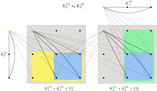
Figure 5: The $2$-join of $K_{2}^{(1)}$ and $K_{3}^{(2)}$, with all the connections. Full lines represent edges within the tensor product graphs plus the starting and ending graph. Dotted lines represent edges among these graphs. $K_{2}^{(1)}\times K_{2}^{(2)}\times\{1\}$ and $K_{2}^{(1)}\times K_{2}^{(2)}\times\{2\}$ are two copies of the tensor product $K_{2}^{(1)}\times K_{2}^{(2)}$.

Figure 6: Representation of the $2$-join of two copies $K_{3}^{(1)}$ and $K_{3}^{(2)}$ of $K_{3}$. Here, for the sake of visibility, only some edges are represented. The yellow node in $K_{3}^{(1)}$ is connected to all nodes in the yellow area of $K_{3}^{(1)}\times K_{3}^{(2)}\times\{1\}$; similarly, the green node in $K_{3}^{(2)}$ is connected to all nodes in the green area of $K_{3}^{(1)}\times K_{3}^{(1)}\times\{2\}$. The blue nodes of $K_{3}^{(1)}\times K_{3}^{(2)}\times\{1,2\}$ are connected to all nodes in the blue areas of $K_{3}^{(1)}\times K_{3}^{(2)}\times\{1,2\}$. Other connections can be deduced by symmetry.

Figure 7: Examples for the $2$-join of graphs.

Given two graphs $G$ and $H$, we aim to define the $r$-join operation $G\star_{r}H$, for any $r\geq 0$. The vertex set $V(G\star_{r}H)$ is defined by $V(G\star_{r}H)=V(G)\cup V(G)\times V(H)\times\{1,\dots,r\}\cup V(H)$. Let

$$E_{1,r}(G\star_{r}H)=\left\{\{(g,h,i),(g^{\prime},h^{\prime},j)\}\ \middle|\ g,g^{\prime}\in V(G),h,h^{\prime}\in V(H),gg^{\prime}\in E(G),hh^{\prime}\in E(H),\lvert i-j\rvert\leq 1\right\}.$$

Furthermore, let

$$E_{0}(G\star_{r}H)=E(G)\cup\left\{\{g,(g^{\prime},h^{\prime},1)\}\ \middle|\ g,g^{\prime}\in V(G),h^{\prime}\in V(H),gg^{\prime}\in E(G)\right\}$$

and

$$E_{r+1}(G\star_{r}H)=E(H)\cup\left\{\{(g,h,t),h^{\prime}\}\ \middle|\ g\in V(G),h,h^{\prime}\in V(H),hh^{\prime}\in E(H)\right\}.$$

Then, the edge set $E(G\star_{r}H)$ is defined by $E(G\star_{r}H)=E_{0}(G\star_{r}H)\cup E_{1,r}(G\star_{r}H)\cup E_{r+1}(G\star_{r}H)$.

An intuitive visualization of this graph follows: take a sequence of $r+2$ disjoint copies $(G\times H)_{0},(G\times H)_{1},\dots,(G\times H)_{r+1}$ of the tensor product $G\times H$ (an example of a tensor product graph is given in Fig. 4). Clearly, for any $0\leq i\leq r$, there is an isomorphism $f_{i}:(G\times H)_{i}\to(G\times H)_{i+1}$. Then, any two nodes $(g,h)\in(G\times H)_{i}$ and $(g^{\prime},h^{\prime})\in(G\times H)_{i+1}$ are connected if and only if $\{f_{i}((g,h)),(g^{\prime},h^{\prime})\}\in E((G\times H)_{i+1})$, or, equivalently, $\{(g,h),f_{i}^{-1}((g^{\prime},h^{\prime}))\}\in E((G\times H)_{i})$. Finally, “collapse” $(G\times H)_{0}$ into $G$ and $(G\times H)_{r+1}$ into $H$ by merging nodes (merging multiple edges and deleting self-loops).

This join operation in graphs is some kind of “discrete” variant of the join operation between two topological spaces (see [16] or [56]).

We define two projection operators for the join of graphs.

Definition 5.9.

Let $\operatorname{pr}_{G}:G\star_{r}H\setminus H\to G$ and $\operatorname{pr}_{H}:G\star_{r}H\setminus G\to H$ be defined as follows: $\operatorname{pr}_{G}((g,h,i))=g$ and $\operatorname{pr}_{H}((g,h,i))=h$ for $(g,h,i)\in V(G)\times V(H)\times\{1,\dots,r\}$, while $\operatorname{pr}_{G}\restriction_{G}$ and $\operatorname{pr}_{H}\restriction_{H}$ are the identity maps on $G$ and $H$, respectively.

Remark 4.

The two projections are homomorphisms, implying that the chromatic number of $G\star_{r}H\setminus H$ is the same as that of $G$, and the chromatic number of $G\star_{r}H\setminus G$ is the same as that of $H$.

The join of two connected graphs results in a connected graph.

Lemma 5.10.

Let $r\geq 1$, and let $G$ and $H$ be two connected graphs with at least two nodes each. Then, $G\star_{r}H$ is connected.

Proof.

Consider any node $u$ in $G\star_{r}H$ which does not belong to $G\cup H$. Then $u=(g,h,i)$ for $g\in V(G)$, $h\in V(H)$, and $i\in[r]$. There exist $g^{\prime}\in V(G)$ and $h^{\prime}\in V(H)$ such that $gg^{\prime}\in E(G)$ and $hh^{\prime}\in E(H)$. We now construct two paths $v_{0}v_{1}\dots v_{i}$ and $w_{r+1}w_{r}\dots w_{i}$ that connect $G$ and $H$ to $v_{i}=w_{i}=u$, respectively. Suppose $i$ is odd. Then, set $v_{0}=g^{\prime}$, $v_{j}=(g,h,j)$ for any odd $j$, and $v_{j}=(g^{\prime},h^{\prime},j)$ for any even $j$. We have that $v_{j}$ is connected to $v_{j+1}$ for any $0\leq j\leq i-1$, and $v_{i}=u$. Similarly, set $w_{r+1}=h^{\prime}$, $w_{j}=(g,h,j)$ for any odd $j$, and $w_{j}=(g^{\prime},h^{\prime},j)$ for any even $j$. We have that $w_{j}$ is connected to $w_{j-1}$ for any $i+1\leq j\leq r+1$, and $w_{i}=u$. Suppose $i$ is even. Then, set $v_{0}=g$, $v_{j}=(g^{\prime},h^{\prime},j)$ for any odd $j$, and $v_{j}=(g,h,j)$ for any even $j$. We have that $v_{j}$ is connected to $v_{j+1}$ for any $0\leq j\leq i-1$, and $v_{i}=u$. Similarly, set $w_{r+1}=h$, $w_{j}=(g^{\prime},h^{\prime},j)$ for any odd $j$, and $w_{j}=(g,h,j)$ for any even $j$. We have that $w_{j}$ is connected to $w_{j-1}$ for any $i+1\leq j\leq r+1$, and $w_{i}=u$. ∎

We are ready to define the graph from Theorem 5.8 which we will prove to be a cheating graph for the family of $\chi$-chromatic graphs.

Definition 5.11 (The construction).

Let $\chi\geq 2$, $r\geq 2$, and $k\geq 1$. Consider a sequence $K_{\chi}^{(1)},\dots,K_{a}^{(k)}$ of $k$ disjoint copies of $K_{\chi}$. We construct the graph recursively. Let $G_{1}=K_{\chi}^{(1)}$ be the clique with $\chi$ nodes. Then, for $k\geq 2$, $G_{k}=G_{k-1}\star_{2r}K_{\chi}^{(k)}$. [16] proved that $\mathcal{L}\mathcal{X}_{r}(G_{k})=\chi$, $\mathcal{X}(G_{k})\geq k(\chi-1)+1$, and

$$\lvert V(G_{k})\rvert=\frac{(2r\chi+1)^{k}-1}{2r}.$$

See Fig. 7 for some examples (notice that $r=1$ in the examples: as observed in Remark 3, the result still holds in this case).

Further discussion on $G_{k}$ is deferred to Section 5.3.1. In order to continue, we state the following lemma for an induced subgraph, whose proof is trivial.

Lemma 5.12.

Let $T\in\mathbb{N}$. Let $G$ be a connected graph, and $H\subseteq G$ be a connected subgraph of $G$. Then, $G[{\mathcal{N}_{T}(H)}]$ is connected.

For a graph $G$ and any node $v\in V(G)$, we define by $\operatorname{dist}_{G}(v,H)=\min_{u\in V(H)}\left\{\operatorname{dist}_{G}(u,v)\right\}$ the distance between $v$ and any subgraph $H\subseteq G$. We write $\operatorname{dist}(v,H)$ when the underlying graph $G$ is clear from the context. We now prove some key-properties of $G_{k}$ which allow us to show that $G_{k}$ is a cheating graph.

Lemma 5.13.

Let $\chi\geq 2$, $r\geq 3$, and $k\geq 2$ be integers. Define $T=\lfloor\frac{2r}{3}\rfloor$. Let $G_{k}$ be the graph defined in Definition 5.11 built with copies of $K_{\chi}$. There exists a subgraph cover $\{G_{k}^{(i)}\}_{i\in[k]}$ of $G_{k}$ such that the following statements hold:

1. The chromatic number of $G_{k}[{\mathcal{N}_{T}(G_{k}^{(i)})}]$ is $\chi$ for all $i\in[k]$;

2. $G_{k}^{(i)}$ is connected for all $i\in[k]$;

3. for each $v\in V(G_{k})$, there exists $i\in[k]$ such that $\mathcal{N}_{1}(v)\subseteq V(G_{k}^{(i)})$;

4. $G_{k}[\mathcal{N}_{T}(G_{k}^{(i)})]$ contains at least one node at distance $T$ from $G_{k}^{(i)}$ for all $i\in[k]$.

Proof.

We prove the thesis by induction on $k$. Remember that $G_{2}$ is obtained by the $2r$-join of two disjoint copies $K_{\chi}^{(1)}$, $K_{\chi}^{(2)}$ of $K_{\chi}$. Assume $K_{\chi}^{(1)}$ is connected to the first copy of $K_{\chi}^{(1)}\times K_{\chi}^{(2)}$, and $K_{\chi}^{(2)}$ to the last. Let

$$V_{2}^{(1)} =V(K_{\chi}^{(1)})\cup V(K_{\chi}^{(1)})\times V(K_{\chi}^{(2)})\times\left\{1,\dots,T+2\right\};$$

$$V_{2}^{(2)} =V(K_{\chi}^{(2)})\cup V(K_{\chi}^{(1)})\times V(K_{\chi}^{(2)})\times\left\{T+1,\dots,2r\right\}.$$

Consider the graphs $G_{2}^{(1)}=G_{2}[{V_{2}^{(1)}}]$ and $G_{2}^{(2)}=G_{2}[{V_{2}^{(2)}}]$. The cover property and properties (i)-(iii) are straightforward. Clearly, $G_{2}=\cup_{i\in[2]}\ G_{2}^{(i)}$. Furthermore, $\mathcal{X}(G_{2}[{\mathcal{N}_{T}(G_{2}^{(1)})}])=\mathcal{X}(G_{2}[{\mathcal{N}_{T}(G_{2}^{(2)})}])=\chi$ as the projections $\operatorname{pr}_{K_{\chi}^{(1)}}[{\mathcal{N}_{T}(G_{2}^{(1)})}],\operatorname{pr}_{K_{\chi}^{(2)}}[{\mathcal{N}_{T}(G_{2}^{(2)})}]$ are homomorphisms. Moreover, it is easily verifiable that $G_{2}^{(1)}$ and $G_{2}^{(2)}$ are connected graphs: Observe that $G_{2}^{(1)}=(K_{\chi}^{(1)}\star_{2r}K_{\chi}^{(2)})[{\mathcal{N}_{T+2}(K_{\chi}^{(1)})}]$. As both $K_{\chi}^{(1)}$ (by the inductive hypothesis) and $K_{\chi}^{(2)}$ are connected, Lemma 5.10 implies their join is connected. Then, Lemma 5.12 implies $G_{2}^{(1)}$ is connected. The same applies for $G_{2}^{(2)}$ by observing that $G_{k}^{(2)}=(K_{\chi}^{(1)}\star_{2r}K_{\chi}^{(2)})[{\mathcal{N}_{2r-T}(K_{\chi}^{(2)})}]$. As for property (iv), consider any two nodes $u\in V(K_{\chi}^{(1)})\times V(K_{\chi}^{(2)})\times\left\{2T+2\right\}$ and $v\in V(K_{\chi}^{(1)})\times V(K_{\chi}^{(2)})\times\left\{1\right\}$. Clearly, $u\in G_{2}[\mathcal{N}_{T}(G_{2}^{(1)})]$ and has distance $T$ from $G_{2}^{(1)}$, while $v\in G_{2}[\mathcal{N}_{T}(G_{2}^{(2)})]$ and has distance $T$ from $G_{2}^{(2)}$.

Let $k\geq 3$ and assume the thesis is true for $G_{k-1}$. We now construct the subgraph cover of $G_{k}=G_{k-1}\star_{2r}K_{\chi}$. For $i=1,\dots,k-1$, we define $G_{k}^{(i)}$ by

$$G_{k}^{(i)}=G_{k-1}^{(i)}\cup\left(G_{k}[{\mathcal{N}_{T+2}(G_{k-1}^{(i)})}]\ \cap\ G_{k}[{V(G_{k-1}^{(i)})\times V(K_{\chi}^{(k)})\times\{1,\dots,T+2\}}]\right)$$

Then, we define

$$G_{k}^{(k)}=G_{k}[{V(G_{k-1})\times V(K_{\chi}^{(k)})\times\{T+1,\dots,2r\}}]\cup K_{\chi}^{(k)}.$$

We now prove that the family $\{G_{k}^{(i)}\}_{i\in[k]}$ respects properties (i)-(iv).

Subgraph covering.

Any node $v\in(V(G_{k-1})\cup V(K_{\chi}^{(k)}))$ belongs either to $(\cup_{i\in[k-1]}G_{k}^{(i)})$ (by observing that the latter contains $V(G_{k-1})$ and by using the inductive the hypothesis on the subgraph covering) or to $G_{k}^{(k)}$ (which contains $V(K_{\chi}^{(k)})$ by construction). Consider any node $v\in V(G_{k})\setminus(V(G_{k-1})\cup V(K_{\chi}^{(k)}))$. Then $v=(v_{1},v_{2},j)$ for $v_{1}\in V(G_{k-1})$, $v_{2}\in V(K_{\chi}^{(k)})$, and $j\in[2r]$. By the inductive hypothesis, there exists $i\in[k-1]$ such that $v_{1}\in G_{k-1}^{(i)}$. Then, $(v_{1},v_{2},j)\in V(G_{k-1}^{(i)})\times V(K_{\chi}^{(k)})\times\{j\}$. As $G_{k-1}^{(i)}$ and $K_{\chi}^{(k)}$ contain no isolated nodes (inductive hypothesis (ii)), there exist $u_{1}\in V(G_{k-1}^{(i)})$ adjacent to $v_{1}$ and $u_{2}\in V(K_{\chi}^{(k)})$ adjacent to $v_{2}$. The path $w_{0}w_{1}\dots w_{j}$ defined by $w_{0}=u_{1}$, $w_{k}=(v_{1},v_{2},k)$ for $1\leq k\leq j$ odd, $w_{k}=(u_{1},u_{2},k)$ for $2\leq k\leq j$ even connects $u_{1}$ to $v$ if $j$ is odd. The path $w_{0}w_{1}\dots w_{j}$ defined by $w_{0}=v_{1}$, $w_{k}=(u_{1},u_{2},k)$ for $1\leq k\leq j$ odd, $w_{k}=(v_{1},v_{2},k)$ for $2\leq k\leq j$ even connects $v_{1}$ to $v$ if $j$ is even. Hence, $v\in\mathcal{N}_{j}(G_{k-1}^{(i)})$. If $1\leq j\leq T+2$, then $u\in V(G_{k}^{(i)})$. If, instead, $T+2\leq j\leq 2r$, then $u\in V(G_{k}^{(k)})$.

Now consider any two nodes $u,v$ which are connected in $G_{k}$. If $u,v\in V(G_{k-1})$ or $u,v\in V(K_{\chi}^{(k)})$ we have that $\{u,v\}\in E(\cup_{i\in[k-1]}G_{k}^{(i)})$ or $\{u,v\}\in E(G_{k}^{(k)})$, respectively. Suppose $u\in V(G_{k-1})$ but $v\notin V(G_{k-1})$. Then, $v=(v_{1},v_{2},1)$ for some $v_{1}\in V(G_{k-1})$ and some $v_{2}\in V(K_{\chi}^{(k)})$. As $u$ and $v$ are connected, it means that $uv_{1}$ is an edge in $G_{k-1}$. By the inductive hypothesis on the subgraph covering, there exists $i\in[k-1]$ such that $uv_{1}\in G_{k-1}^{(i)}$. Hence, $uv\in E(G_{k}^{(i)})$. If $u\in V(K_{\chi}^{(k)})$ but $v\notin V(K_{\chi}^{(k)})$, $uv\in E(G_{k}^{(k)})$. Suppose now that $u,v\notin V(G_{k-1})\cup V(K_{\chi}^{(k)})$. Then, there exist $u_{1},v_{1}\in V(G_{k-1})$, $u_{2},v_{2}\in V(K_{\chi}^{(k)})$, and $j_{u},j_{j}\in[2r]$ with $\lvert j_{u}-j_{v}\rvert\leq 1$ such that $u=(u_{1},u_{2},j_{u})$ and $v=(v_{1},v_{2},j_{v})$. Furthermore, as $uv$ is an edge of $G_{k}$, it holds that $u_{1}u_{2}$ is an edge in $G_{k-1}$, and $v_{1}v_{2}$ is an edge in $K_{\chi}^{(k)}$. From the inductive hypothesis on the subgraph covering, there exists $i\in[k-1]$ such that $G_{k-1}^{(i)}$ contains $u_{1}u_{2}$. We have that $u,v\in V(G_{k}[{V(G_{k-1}^{(i)})\times V(K_{\chi}^{(k)})\times\{j_{u},j_{v}\}}])$. Let $j=\max(j_{u},j_{v})$ Then, $uv\in E(G_{k}[{\mathcal{N}_{j}(G_{k-1}^{(i)})}])$. Hence, if $j\leq T+2$, $uv\in E(G_{k}^{(i)})$. If, instead, $T+1\leq j\leq 2r$, $uv\in E(G_{k}^{(k)})$.

Property (i).

Consider $G_{k}^{(i)}$ for $i<k$. The function $f_{i}=\operatorname{pr}_{G_{k-1}}\restriction_{\mathcal{N}_{T}(G_{k}^{(i)})}$ is a homomorphism from $G_{k}[{\mathcal{N}_{T}(G_{k}^{(i)})}]$ to $G_{k-1}[{\mathcal{N}_{T}(G_{k-1}^{(i)})}]$. As $G_{k-1}[{\mathcal{N}_{T}(G_{k-1}^{(i)})}]$ is $\chi$-colorable by the inductive hypothesis (i), so it is $G_{k}[{\mathcal{N}_{T}(G_{k}^{(i)})}]$. Since $G_{k}[{\mathcal{N}_{T}(G_{k}^{(i)})}]$ contains $K_{\chi}^{(i)}$ as a subgraph, $\chi$ colors are also necessary.

Similarly, consider $G_{k}[{\mathcal{N}_{T}(G_{k}^{(k)})}]$. Then, $f_{k}=\operatorname{pr}_{K_{\chi}^{(k)}}\restriction_{[\mathcal{N}_{T}(G_{k}^{(k)})]}$ is a homomorphism from $G_{k}[{\mathcal{N}_{T}(G_{k}^{(k)})}]$ to $K_{\chi}^{(k)}$. Hence, $G_{k}[{\mathcal{N}_{T}(G_{k}^{(k)})}]$ is $\chi$-colorable. As $G_{k}[{\mathcal{N}_{T}(G_{k}^{(k)})}]$ contains $K_{\chi}^{(k)}$, its chromatic number is $\chi$.

Property (ii).

Fix $i\in[k-1]$. Observe that $G_{k}^{(i)}=G_{k-1}^{(i)}\star_{2r}K_{\chi}^{(k)}[{\mathcal{N}_{T+1}(G_{k-1}^{(i)})}]$. As both $G_{k-1}^{(i)}$ (by the inductive hypothesis (ii)) and $K_{\chi}^{(k)}$ are connected, their join is connected. Then, Lemma 5.12 implies that $G_{k}^{(i)}$ is connected. The same applies for $G_{k}^{(k)}$ by observing that $G_{k}^{(i)}=G_{k-1}^{(i)}\star_{2r}K_{\chi}^{(k)}[{\mathcal{N}_{2r-T}(K_{\chi}^{(k)})}]$.

Property (iii).

Consider any node $v\in V(G_{k-1})\cup V(G_{k-1})\times V(K_{\chi}^{(k)})\times\{1,\dots,T+1\}$. Let $v^{\prime}=\operatorname{pr}_{G_{k-1}}({v})$. By the inductive hypothesis (iii), the set of nodes $\mathcal{N}_{1}(v^{\prime})\cap V(G_{k-1})$ is contained in some $G_{k-1}^{(i)}$ for $i\in[k-1]$. By definition of $G_{k}^{(i)}$, it follows that $\mathcal{N}_{1}(v)\subseteq V(G_{k}^{(i)})$. Now, consider any node $v\in V(K_{\chi}^{(k)})\cup V(G_{k-1})\times V(K_{\chi}^{(k)})\times\{T+2,\dotsm 2r\}$. By definition of $G_{k}^{(k)}$, we have that $\mathcal{N}_{1}(v)\subseteq G_{k}^{(k)}$.

Property (iv).

Fix $1\leq i\neq j\leq k-1$. By the inductive hypothesis (iv), there exists a node $u\in V(G_{k-1}[\mathcal{N}_{T}(G_{k-1}^{(i)})])$ from $G_{k-1}^{(i)}$. By definition of $G_{k}^{(i)}$, we have that $u$ has distance $T$ from $G_{k}^{(i)}$. Furthermore, observe that any node in $V(G_{k-1})\times V(K_{\chi}^{(k)})\times{1}$ has distance $T$ from $G_{k}^{k}$, concluding the proof. ∎

Remark 5.

We highlight that the subgraph cover from Lemma 5.13 is not unique: other families of graphs could be used obtaining a shorter and simpler proof at the expense of a higher number of graphs in the family (e.g., a number of subgraphs that is exponential in $k$). The latter would result in a worse bound on $T$ in the next corollary.

We are now ready to show that the family of $\chi$-chromatic graphs admits a cheating graph for the $c$-coloring graphs problem.

Corollary 5.14.

Let $\chi\geq 2$, $c\geq\chi$ be integers, and $k=\lfloor\frac{c-1}{\chi-1}\rfloor$. Consider $\mathcal{F}$ to be the family of all connected $\chi$-chromatic graphs, and $\mathcal{P}$ to be the problem of $c$-coloring graphs. For every $N\geq 1$ and $n\geq((6\chi+1)^{k+1}-1)N/6$, there exists a value $T$ with

$$T=\Theta\!\left(\frac{1}{\chi^{1+\frac{1}{k}}}\left(\frac{n}{N}\right)^{\frac{1}{k}}\right)$$

such that $\mathcal{F}$ admits an $(n,k+1,N,T)$-cheating graph for $\mathcal{P}$.

Proof.

There exists a unique integer $r\geq 3$ such that

$$\frac{(2r\chi+1)^{k+1}-1}{2r}\leq\frac{n}{N}<\frac{(2r\chi+2\chi+1)^{k+1}-1}{2r+2}.$$

We claim that the graph $G_{k+1}$ defined in Definition 5.11 by iterating $2r$-join operations is an $(n,{k+1},N,T)$-cheating graph for $(\mathcal{P},\mathcal{F})$. Clearly, $\mathcal{P}$ is not solvable on $G_{k+1}$, while property Definition 5.6.(ii).(a) follows by Lemma 5.13.(iii) (since coloring is an LVL problem with checking radius $t=1$).

We now prove that Definition 5.6.(ii).(b) holds as well. Consider $N$ copies $G_{{k+1},1}.\dots.G_{{k+1},N}$ of the graph $G_{k+1}$. For each $j\in[N]$, Lemma 5.13 gives us a subgraph cover $\{G_{{k+1},j}^{(i)}\}_{i\in[{k+1}]}$ of $G_{k,j}$ with properties Lemma 5.13.(i) and (iv) verified for $T=\lfloor\frac{2r}{3}\rfloor$. Notice that

$$T=\Theta\!\left(\frac{1}{\chi^{1+\frac{1}{k}}}\left(\frac{n}{N}\right)^{\frac{1}{k}}\right).$$

For any choice of indices $\mathbf{x}_{N}=(x_{1},\dots,x_{N})\in[{k+1}]^{N}$, we now show that there exists a connected graph $H_{\mathbf{x}_{N}}\in\mathcal{F}$ on $n$ nodes that admits a subgraph $\tilde{H}_{\mathbf{x}_{N}}$ such that

1. $H_{\mathbf{x}_{N}}[{\mathcal{N}_{T}(\tilde{H}_{\mathbf{x}_{N}})}]$ is isomorphic to $\bigsqcup_{j\in[N]}G_{{k+1},j}[{\mathcal{N}_{T}(G_{{k+1},j}^{(x_{j})})}]$;

2. $\mathcal{X}(H_{\mathbf{x}_{N}})=\chi$.

The vertex set $V(H_{\mathbf{x}_{N}})$ is $V(\sqcup_{j\in[N]}G_{{k+1},j})$ together with $n-N\cdot\frac{(2r\chi+1)^{k+1}-1}{2r}\leq\frac{n}{N}$ extra nodes. We take $H_{\mathbf{x}_{N}}$ to be the disjoint union of $G_{{k+1},j}[{\mathcal{N}_{T}(G_{{k+1},j}^{(x_{j})})}]$ for all $j\in[N]$ where, for each $j\in[N-1]$ we add an edge between a node $v_{j}\in G_{{k+1},j}[{\mathcal{N}_{T}(G_{{k+1},j}^{(x_{j})})}]$ and a node $v_{j+1}\in G_{{k+1},j+1}[{\mathcal{N}_{T}(G_{{k+1},j+1}^{(x_{j+1})})}]$ such that $\operatorname{dist}(v_{j},G_{{k+1},j}^{(x_{j})})=T$ and $\operatorname{dist}(v_{j+1},G_{{k+1},{j+1}}^{(x_{j+1})})=T$ (such nodes exist because of Lemma 5.13.(iv)). All remaining nodes form a path of which one endpoint is connected to any node in $G_{{k+1},N}[\mathcal{N}_{T}({G_{{k+1},N}^{(x_{N})}})]$ at distance $T$ from ${G_{{k+1},N}^{(x_{N})}}$. Property (1) follows by construction. As for property (2), we observe that the chromatic number of $H_{\mathbf{x}_{N}}$ is still $\chi$ as each component $\mathcal{N}_{T}(G_{{k+1},j}^{(x_{j})})$ is $\chi$-chromatic by Lemma 5.13.(i), and $\chi\geq 2$. Furthermore, $H_{\mathbf{x}_{N}}$ is connected by Lemma 5.13.(ii) combined with Lemma 5.12 and observing that connected disjoint connected components through paths. ∎

The proof of our main lower bound now follows easily.

Proof of Theorem 1.3.

Let $k=\alpha$ and

$$N=\left\lceil\frac{\log\frac{1}{\varepsilon}}{\log\left(1+\frac{1}{k}\right)}\right\rceil.$$

By Corollary 5.14, $\mathcal{F}$ admits an $(n,{k+1},N,T)$-cheating graph for the $c$-coloring graphs problem for any $n\geq((6\chi+1)^{k+1}-1)N/6$ and for some

$$T=\Theta\!\left(\frac{1}{\chi^{1+\frac{1}{k}}}\cdot\left(\frac{n\log(1+\frac{1}{k})}{\log\frac{1}{\varepsilon}}\right)^{\frac{1}{k}}\right).$$

Theorem 5.7 implies that there is a connected graph $H\in\mathcal{F}$ on $n$ nodes such that the probability that any outcome $\mathrm{O}$ with locality $T$ is $c$-coloring $H$ is at most $(1-1/(k+1))^{N}$. We remind the reader that the graph can be chosen as in Definition 5.6.(ii).(b), and Corollary 5.14 implies that such graph is connected. By definition of $k$ and $N$, this probability is at most $\varepsilon$. By observing that $\log^{\frac{1}{k}}(1+\frac{1}{k})=\Theta(1)$, we get the thesis. ∎

5.3.1 Notes on the graph $G_{k}$

This section is dedicated to the reader that is interested in the topological elements underlying the construction of the graph $G_{k}$ in [16]. Familiarity with the notion of topological space, join of topological spaces, homotopy equivalence, abstract simplicial complex, and geometric realization of an abstract simplicial complex is required. Every graph $G$ can be associated with an abstract simplicial complex $NC\!\left(G\right)$ called the neighborhood complex, defined as follows:

$$NC\!\left(G\right)\coloneqq\left\{A\subseteq V(G)\ \middle|\ \exists v\in V(G)\text{ such that }\forall u\in A,v\in\mathcal{N}(u)\right\},$$

that is, $NC\!\left(G\right)$ consists in all subsets $A\subseteq V$ of nodes that have a common neighbor. Let us denote the geometric realization of $NC\!\left(G\right)$ by $\lVert NC\!\left(G\right)\rVert$ (the geometric realization is unique up to homeomorphisms). We say that a non-empty topological space $X$ is $m$-connected if each continuous map $\pi:S^{i-1}\to X$ extends to a continuous map $\bar{\pi}:D^{i}\to X$ for each $i=1,\dots,m$, where $S^{i-1}=\left\{x\in^{i}\ \middle|\ \lVert x\rVert_{2}=1\right\}$ is the $(i-1)$-dimensional sphere, and $D^{i}=\left\{x\in^{i}\ \middle|\ \lVert x\rVert_{2}\leq 1\right\}$ is the $i$-dimensional disk.

[51] proved the following theorem.

Theorem 5.15 ([51]).

Let $G$ be any graph such that $NC\!\left(G\right)$ is non-empty. If $\lVert NC\!\left(G\right)\rVert$ is $m$-connected, then $\mathcal{X}(G)\geq m+3$.

[51]’s result provides a clear and effective tool to bound from below the chromatic number of a graph. [16] linked the $r$-join operation between graphs to the join operation of topological spaces, proving the following lemma.

Lemma 5.16 ([16]).

Let $G,H$ be any two graphs, and $r\in\mathbb{N}_{+}$. Then, $\lVert NC\!\left(G\star_{r}H\right)\rVert\simeq\lVert NC\!\left(G\right)\rVert\star\lVert NC\!\left(H\right)\rVert$, where $\simeq$ means homotopy equivalent and the latter $\star$ operator represents the join operation between topological spaces.

Note that, for any three topological spaces $A$, $A^{\prime}$, and $B$, if $A\simeq A^{\prime}$, then $A\star B\simeq A^{\prime}\star B$ [56]. Theorems 5.15 and 5.16 can be combined to construct graphs of high chromatic number. E.g., if $G=K^{(1)}_{\chi}$ and $H=K^{(2)}_{\chi}$, that is, two disjoint copies of the complete graph of $\chi$ nodes, we know that $\lVert NC\!\left(G\right)\rVert\simeq\lVert NC\!\left(H\right)\rVert\simeq S^{\chi-2}$, hence $\lVert NC\!\left(G\star_{r}H\right)\rVert\simeq S^{\chi-2}\star S^{\chi-2}\simeq S^{2\chi-3}$. As $S^{2\chi-3}$ is $(2\chi-4)$-connected, then $\mathcal{X}(G\star_{r}H)\geq 2\chi-1$. By applying recursively the above procedure, one can understand why the graph $G_{k}$ from Definition 5.11 has chromatic number bounded from below by $k(\chi-1)+1$.

As for the properties of the local chromatic number, [16] also showed the following simple result, which can be proved by using the projections $\operatorname{pr}_{G}$ and $\operatorname{pr}_{H}$, that immediately gives the desired result.

Lemma 5.17 ([16]).

Let $G,H$ be two graphs. For every $r\in\mathbb{N}_{+}$ it holds that

$$\mathcal{L}\mathcal{X}_{r}{(G\star_{2r}H)}=\min\{\mathcal{L}\mathcal{X}_{r}(G),\mathcal{L}\mathcal{X}_{r}(H)\}.$$

5.3.2 On highly chromatic graphs with small local chromatic number

In this section we present previous works studying the relation between the chromatic number and the local chromatic number of a graph. We remind to the reader that the local chromatic number $\mathcal{L}\mathcal{X}_{r}(G)$ of radius $r$ of a graph $G$ is the maximum number of colors required to color any $r$-ball in $G$. We remark that, in this paper, we depart from the standard definition of local chromatic number in the literature that started with [29], which is not useful for our purposes. For positive integers $c,\chi,r$, define $f_{\chi}(c,r)$ to be the maximal integer $n$ such that every graph $G$ of $n$ nodes with $\mathcal{L}\mathcal{X}_{r}(G)\leq\chi$ is $c$-colorable. The first bounds on $f_{\chi}(c,r)$ held for specific values of $\chi$, especially $\chi\in\{2,3\}$ [28, 62, 14] (for a summary of the progress of such results we defer the reader to [17, 3]). We only describe the results that consider a generic $\chi$, as they are more directly related to our work. [44] proved that, for each $k\in\mathbb{N}$,

$$f_{\chi}(k(\chi-1)+1,r)\geq\lfloor r/(2k)\rfloor^{k},$$ (1)

i.e., any graph $G$ having $\mathcal{L}\mathcal{X}_{r}(G)\leq\chi$ and $\lvert V\rvert\leq\lfloor r/(2k)\rfloor^{k}$ has chromatic number at most $k(\chi-1)+1$. Thirty years later, [16] proved that this result is basically tight when $k,\chi$ are fixed: it showed that, for each $k\geq 2$,

$$f_{\chi}(k(\chi-1),r)\leq\frac{(2r\chi+1)^{k}-1}{2r},$$ (2)

i.e., there exists a graph $G_{k}$ with $\mathcal{L}\mathcal{X}_{r}(G_{k})=\chi$, $\mathcal{X}(G_{k})\geq k(\chi-1)+1$, and $\lvert V(G_{k})\rvert=\frac{(2r\chi)^{k}-1}{2r}$: such result is built upon a lemma by [51]. The two above results show an interesting phenomenon. For constant positive integers $\chi$ and $c$, the minimum number of vertices of a graph $G$ with $\mathcal{L}\mathcal{X}_{r}(G)\leq\chi$ and $\chi(G)=c$ is roughly $r^{\lfloor\frac{c-1}{\chi-1}\rfloor}$, that is, it jumps to the powers of $r$ where the exponents are the values $c$ congruent to $1$ modulo $\chi-1$.

The estimate by [44] breaks when $k\gtrsim r$. [17] and [3] investigated and provided better lower bounds to $f_{\chi}(c,r)$ when $c\gtrsim(\chi-1)r$; [3] estimated also upper bounds to $f_{\chi}(c,r)$ which are roughly tight for fixed $r$. We do not discuss such results in details as they are not useful for our purposes: we are interested in the asymptotic relation between the locality radius $r$ and the number of nodes $n$ given the local and global chromatic number. Such case is covered by Eq. 2: in particular, we used the example graph that was built in [16] as our baseline for the lower bound proof.

We remark that our result for the specific case $\chi=2$ could also be achieved through other graphs that were studied in the literature, e.g., the generalized Mycielski graph (studied by [62], see [37] for an English version of the proof).

5.4 No quantum advantage for $3$-coloring grids

In this section we prove that $3$-coloring $n_{1}\times n_{2}$ grids of requires time $\Omega\!\left(\min(n_{1},n_{2})\right)$ rounds in the $\operatorname{\mathsf{NS-LOCAL}}$ model, by using the same graph-theoretical lower bound argument of Section 5.

For any two integers $a\leq b$, we denote the set $\{a,a+1,\dots,b\}$ by $[a:b]$.

Definition 5.18 (KB-gadget).

Consider a graph $H_{n_{1},n_{2}}=(V(H_{n_{1},n_{2}}),E(H_{n_{1},n_{2}}))$ of $(n_{1}+1)(n_{2}+1)$ nodes, where we label the nodes by using coordinates from the set $[0:n_{1}]\times[0:n_{2}]$; two nodes $(i,j)$ and $(i^{\prime},j^{\prime})$ are connected by an edge if $\lvert i-i^{\prime}\rvert+\lvert j-j^{\prime}\rvert=1$, i.e., their Manhattan distance is 1. Now, define the following equivalence relation for nodes: $(i,0)\sim_{V}(n_{1}-i,n_{2})$ for $i=0,\dots,n_{1}$, and $(0,j)\sim_{V}(n_{1},j)$ for $j=0,\dots,n_{2}$. Now define a new graph $G_{n_{1},n_{2}}=(V(G_{n_{1},n_{2}}),E(G_{n_{1},n_{2}}))$ where $V(G_{n_{1},n_{2}})=V(H_{n_{1},n_{2}})/{\sim_{V}}$ and $E(G_{n_{1},n_{2}})$ is characterized as follows: Take any two nodes $u,v\in V(G_{n_{1},n_{2}})$. Such nodes are equivalence classes for $\sim_{V}$. If there exists $u^{\prime}\in u\subseteq V(H_{n_{1},n_{2}}),v^{\prime}\in u\subseteq V(H_{n_{1},n_{2}})$ such that $u^{\prime}v^{\prime}\in E(H_{n_{1},n_{2}})$, then $uv\in E(G_{n_{1},n_{2}})$ (see Fig. 8). We name $G_{n_{1},n_{2}}$ an $n_{1}\times n_{2}$ Klein bottle gadget (KB-gadget).

Now, clearly, $G_{n_{1},n_{2}}$ is everywhere locally grid-like; however, we claim that $\mathcal{X}(G)\geq 4$ if $n_{1}$ is odd.

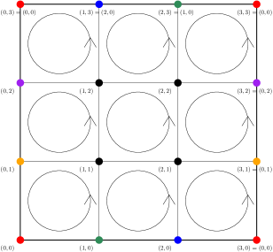
Figure 8: Representations of graphs $G_{n_{1},n_{2}}$ and $H_{n_{1},n_{2}}$ with $n_{1}=n_{2}=3$. Nodes on the borders are identified in $G_{n_{1},n_{2}}$ as indicated by the same colors. Each face of the graph is oriented the same as the oriented circle inside it.

Quadrangulation of the Klein bottle.

To establish the truth of our claim, we make use of results on the chromatic number of quadrangulations of surfaces [5, 58, 59]. Following the preliminaries of [59], by surface we mean a compact connected 2 manifold without boundary. A quadrangulation of a surface is a graph without self-loops on that surface with all faces being quadrilaterals. For our purpose, we can restrict to the class of simple graphs. Let $G$ be a quadrangulation of a surface $S$. An orientation of a face of $G$ is a closed walk along its boundaries. Given two oriented faces sharing at least one boundary edge $e$, we say that the consistency of the orientation is not broken at $e$ if we traverse edge in opposite directions when considering the two orientations of the faces. Given an arbitrary orientation of all faces we can count the edges that break consistency of the orientation of the surface. Note that reversing the orientation of a face changes the status of its four edges, and thus the parity of the number of edges breaking consistency does not change. We say that $G$ is even or odd depending on this parity. By the previous remark, the parity of the quadrangulation is determined by any orientation of all faces and is invariant, i.e., it depends only on the graph $G$.

The following theorem was independently proved by [5, 58], but we report its formulation by [59].

Theorem 5.19 ([59]).

Let $G$ be an odd quadrangulation of some surface $S$. Then, $\mathcal{X}(G)\geq 4$.

The Klein bottle can be defined as the quotient space of the square $[0,1]\times[0,1]$ over the equivalence relation $\sim$ that identifies sides as follows: $(x,0)\sim(x,1)$ for $x\in[0,1]$, and $(0,y)\sim(1,1-y)$ for $y\in[0,1]$.

Lemma 5.20.

Let $n_{2}\geq 2$. For any odd integer $n_{1}\geq 3$, $\mathcal{X}(G_{n_{1},n_{2}})\geq 4$ and $\mathcal{X}(G_{n_{2},n_{1}})\geq 4$.

Proof.

Notice that $G_{n_{2},n_{1}}$ is isomorphic to $G_{n_{1},n_{2}}$, hence we focus on the latter. It is easy to see that $G_{n_{1},n_{2}}$ is a quadrangulation of the Klein-bottle. Indeed, $H_{n_{1},n_{2}}$ is a quadrangulation of the square $[0,1]\times[0,1]$: it suffices to map the nodes $(i,j)$ into $(i/n_{1},j/n_{2})$, for all $i,j$. As $G_{n_{1},n_{2}}$ is obtained by node identification through the relation $\sim_{V}$, which acts on the border of the square, we have a quadrangulation of the Klein-bottle. Let’s orient the faces of $G_{n_{1},n_{2}}$ as in Fig. 8. Even though in $H_{n_{1},n_{2}}$ the orientation is even as consistency is never broken, through simple observations, one can verify that $G_{n_{1},n_{2}}$ is an odd quadrangulation if and only if $n$ is odd, as the orientation consistency is broken only at edges belonging to the set $\left\{\{(i,0),(i+1,0)\}\ \middle|\ 0\leq i\leq n_{1}-1\right\}$. Then Theorem 5.19 gives the thesis. ∎

It suffices to construct a suitable subgraph cover for $G_{n_{1},n_{2}}$ which shows that the family of grid graphs admits cheating graphs for the 3-coloring problem. First, let us denote by $Q_{n_{1},n_{2}}$ any subgraph of the infinite two-dimensional lattice that is isomorphic to an $(n_{1}+5)/2\times(n_{2}+5)/2$ grid, and by $Q_{n_{1},n_{2}}^{T}$ the graph induced by its $T$-neighborhood in the lattice.

Lemma 5.21.

Let $5\leq n_{1},n_{2}$ be odd integers, and let $G_{n_{1},n_{2}}$ be the graph defined in Definition 5.18. Let $T=\lfloor\frac{\min(n_{1},n_{2})-5}{4}\rfloor$. There exists a subgraph cover $\{G_{n_{1},n_{2}}^{(i)}\}_{i\in[4]}$ of $G_{n_{1},n_{2}}$ such that the following statements hold:

1. The chromatic number of $G_{n_{1},n_{2}}[\mathcal{N}_{T}(G_{n_{1},n_{2}}^{(i)})]$ is 2 for $i\in[4]$;

2. $G_{n_{1},n_{2}}[\mathcal{N}_{T}(G_{n_{1},n_{2}}^{(i)})]$ is isomorphic to $Q_{n_{1},n_{2}}^{T}$;

3. For each $v\in V(G_{n_{1},n_{2}})$, there exists $i\in[4]$ such that $\mathcal{N}_{1}(v)\subseteq V(G_{n_{1},n_{2}}^{(i)})$.

Proof.

Observe that claim (ii) implies claim (i): hence, we prove claim (ii). Consider the graph $H_{n_{1},n_{2}}$ used to construct the KB-gadget in Definition 5.18. Let $V_{1}$ be the set of nodes $(i,j)$ of $H_{n_{1},n_{2}}$ respecting the following property

$$V_{1}:\ i\in\left[0:\frac{n_{1}+1}{2}\right]\cup[n_{1}-1:n_{1}],j\in\left[0:\frac{n_{2}+1}{2}\right]\text{ or }i\in[0:1]\cup\left[\frac{n_{1}-1}{2}:n_{1}\right],j\in[n_{2}-1:n_{2}].$$

Similarly, we define $V_{2},V_{3},V_{4}$ by the following properties

$$V_{2}: \ i\in[0:1]\cup\left[\frac{n_{1}-1}{2}:n_{1}\right],j\in\left[0:\frac{n_{2}-1}{2}\right]\text{ or }i\in\left[0:\frac{n_{1}+1}{2}\right]\cup[n_{1}-1:n_{1}],j\in[n_{2}-1:n_{2}];$$

$$V_{3}: \ i\in\left[0:\frac{n_{1}+1}{2}\right]\cup[n_{1}-1:n_{1}],j\in[0:1]\text{ or }i\in[0:1]\cup\left[\frac{n_{1}-1}{2}:n_{1}\right],j\in\left[\frac{n_{2}-1}{2}:n_{2}\right];$$

$$V_{4}: \ i\in[0:1]\cup\left[\frac{n_{1}-1}{2}:n_{1}\right],j\in[0:1]\text{ or }i\in\left[0:\frac{n_{1}+1}{2}\right]\cup[n_{1}-1:n_{1}],j\in\left[\frac{n_{2}-1}{2}:n_{2}\right].$$

For an example of $V_{1},V_{2}$ see Fig. 11. Then, define $S_{i}$ to be subset of $V(G_{n_{1},n_{2}})$ induced by $V_{i}$ after applying the equivalence relation $\sim_{V}$ in $V(H_{n_{1},n_{2}})$, and $G_{n_{1},n_{2}}^{(i)}=G_{n_{1},n_{2}}[S_{i}]$. Notice that $G_{n_{1},n_{2}}^{(i)}$ is isomorphic to $Q_{n_{1},n_{2}}$ for each $i\in[4]$. Furthermore, the $T$-view of $G_{n_{1},n_{2}}^{(i)}$ identifies in $H_{n_{1},n_{2}}$ four graphs that do not intersect, implying claim (ii). Claim (iii) is trivial. ∎

Remark 6.

The strange shape of the subgraph cover is needed for property (iii). However, the analysis carries on by considering “simpler” subgraph covers which don’t meet property (iii) as a valid coloring can be checked by looking at single edges, not necessarily entire neighborhoods. Nevertheless, we choose to use the general result for LVLs (Theorem 5.7).

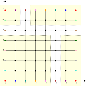
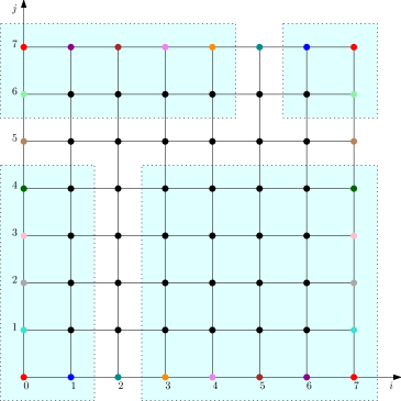
Figure 9: $V_{1}$ (marked in yellow).

Figure 10: $V_{2}$ (marked in blue).

Figure 11: Two elements of the subgraph cover of the KB-gadget for $n_{1}=n_{2}=7$. Nodes with identical colors are identified. $V_{3}$ and $V_{4}$ can be obtained by symmetries.

Lemma 5.21 implies that the family of grid graphs admits cheating graphs for the $3$-coloring graphs problem.

Corollary 5.22.

Let $N\geq 1$, $n_{1},n_{2}\geq 5N$, and $\mathcal{F}$ be the family of all grids of size $n_{1}\times n_{2}$. There exist a $T=T(n_{1},n_{2})$, with

$$T=\Theta\!\left(\frac{1}{N}\cdot\min(n_{1},n_{2})\right),$$

such that $\mathcal{F}$ admits an $(n_{1}\cdot n_{2},4,N,T)$-cheating graph for the $3$-coloring graph problem.

Proof.

Let $M_{1}=\lfloor\frac{n_{1}}{N}\rfloor$ if $\lfloor\frac{n_{1}}{N}\rfloor$ is odd, otherwise $M_{1}=\lfloor\frac{n_{1}}{N}\rfloor-1$. Similarly, let $M_{2}=\lfloor\frac{n_{2}}{N}\rfloor$ if $\lfloor\frac{n_{2}}{N}\rfloor$ is odd, otherwise $M_{2}=\lfloor\frac{n_{2}}{N}\rfloor-1$. Consider the graph $G_{M_{1},M_{2}}$ and the subgraph cover given by Lemma 5.21. Property (i) of Definition 5.6 is clearly satisfied as $\mathcal{X}(G_{M_{1},M_{2}})\geq 4$. Property (ii).(a) is implied by Lemma 5.21 as the checking radius of the coloring problem is $t=1$. Consider now a vertex $v\in V(G_{M_{1},M_{2}})$. Let us now prove property (ii).(b). Consider the subgraph family $\{G_{M_{1},M_{2}}^{(i)}\}_{i\in[4]}$ given by Lemma 5.21: then, $T=\lfloor\frac{1}{4}\cdot(\min(M_{1},M_{2})-5)\rfloor$. Consider any choice of indices $\mathbf{x}_{N}\in[4]^{N}$. Notice that $G_{M_{1},M_{2}}[\mathcal{N}_{T}(G_{M_{1},M_{2}}^{(i)})]$ is isomorphic to $Q^{T}_{M_{1},M_{2}}$ which is, in turn, isomorphic to a proper subgraph of an $M_{1}\times M_{2}$-grid. Hence, it is always possible to construct an $n_{1}\times n_{2}$ grid which respects property (ii).(b) of Definition 5.6. The thesis follows by observing that $T\geq{\frac{1}{4N}\cdot\min(n_{1},n_{2})-3}$. ∎

See 1.4

Proof.

By Corollary 5.22, there exists a $T=\Theta\!\left(\frac{1}{N}\cdot\min(n_{1},n_{2})\right)$ such that the family $\mathcal{F}$ of $n\times m$ grids admits an $(n_{1}\cdot n_{2},4,N,T)$-cheating graph for the problem of 3-coloring graphs. Suppose there is an outcome $\mathrm{O}$ with locality $T$ that $3$-colors $n_{1}\times n_{2}$ grids. By Theorem 5.7 and the choice of $N$,the probability of $\mathrm{O}$ solving the problem on an $n_{1}\times n_{2}$-grid is at most $\varepsilon$. Hence, $T=\Omega\!\left(\frac{\min(n_{1},n_{2})}{\log\frac{1}{\varepsilon}}\right)$. ∎

5.5 No quantum advantage for $c$-coloring trees

[49] showed that $c$-coloring trees requires time $\Omega\!\left(\log_{c}n\right)$ in the classical setting. In this section we prove that the problem has roughly the same complexity in the $\operatorname{\mathsf{NS-LOCAL}}$ model, by combining our lower bound technique (Theorem 5.7) and the same graph-theoretical argument used in [49].

For any graph $G$, we define the girth of $G$ to be the length of the shortest cycle contained in $G$; if $G$ contains no cycle, then its girth is infinite. We denote the girth of a graph $G$ by $\operatorname{girth}\!\left(G\right)$. By $\operatorname{diam}\!\left(G\right)$ we denote the diameter of the graph $G$, i.e., the quantity $\max_{u,v\in V(G)}\operatorname{dist}_{G}(u,v)$. The argument followed by [49] uses the following graph-theoretical result.

Lemma 5.23 (Ramanujan graphs, [52]).

Let $p,q$ be two primes that are congruent to 1 modulo 4. If $p\pmod{q}$ is a perfect square, there exists a $d$-regular graph $G$ on $n=q(q^{2}-1)$ nodes with $d=p+1$, which satisfies the following properties:

1. $\operatorname{girth}\!\left(G\right)>2\log_{p}q$;

2. $\operatorname{diam}\!\left(G\right)\leq 2(\log_{p}n+\log_{p}2)+1$;

3. $\mathcal{X}(G)\geq\frac{1}{2}\sqrt{d}$.

We make use of a result in number theory.

Lemma 5.24 (Dirichlet’s theorem on arithmetic progressions).

Let $a,d$ two coprime positive integers. There are infinitely many primes $p$ of the form $p=dm+a$ for some integer $m\geq 0$.

We use the above result to prove the following.

Corollary 5.25.

The following statements hold:

1. There exists a constant $\lambda$ such that, for each $n\geq 1$, there is a prime $p\in[n+1:(1+\lambda)n]$ such that $p\equiv 1\pmod{4}$;

2. If $p$ is a prime such that $p\equiv 1\pmod{4}$, there exist infinitely many primes $q$ such that $q\equiv 1\pmod{4}$ and $p\pmod{q}$ is a non-zero perfect square;

Proof.

For the first result, we follow the same approach of [64]. Let $a\in\mathbb{N},b\in\mathbb{N}_{+}$. Consider the arithmetic progression defined by $s_{n}=a+bn$, for $n\geq 1$. Let

$$\pi_{a,b}(x)=\lvert\left\{p\ \middle|\ p\leq x,\,p\text{ is prime},\,p\equiv a\!\pmod{b}\right\}\rvert.$$

By the prime number theorem for arithmetic progression, we know that

$$\lim_{n\to+\infty}\frac{\pi_{a,b}(n)}{\frac{n}{\varphi(b)\log n}}=1,$$

where $\varphi(x)$ is the Euler’s totient function. Let now

$$\rho_{a,b}(n)=\lvert\left\{k\leq n\ \middle|\ s_{k}\text{ is prime}\right\}\rvert.$$

It holds that $\rho_{a,b}(n)=\pi_{a,b}(a+bn)-\pi_{a,b}(a)$. Then,

$$\lim_{n\to+\infty}\frac{\rho_{a,b}(n)}{\frac{a+bn}{\varphi(b)\log(a+bn)}-\pi_{a,b}(a)}=\lim_{n\to+\infty}\frac{\rho_{a,b}(n)}{\frac{bn}{\varphi(b)\log(bn)}}=1.$$

Let $\lambda>0$ be any constant: then,

$$\lim_{x\to+\infty}{\rho_{a,b}((1+\lambda)x)}-{\rho_{a,b}(x)}=+\infty.$$

Define $n_{\lambda}$ to be the smallest natural number such that ${\rho_{a,b}((1+\lambda)n)}-{\rho_{a,b}(n)}>0$ for all $n\geq n_{\lambda}$. Notice that the function $\lambda\mapsto n_{\lambda}$ is monotone non-increasing and tends to (actually, reaches) 1 as $\lambda$ tends to $+\infty$: by choosing $\lambda$ large enough, one obtains $n_{\lambda}=1$. Hence, there is a value $\lambda=\lambda(a,b)$ such that, for each $n\geq 1$, there is a prime $p\in[n+1:(1+\lambda)n]$ that is congruent to $a$ modulo $b$. Setting $a=1$, $b=4$ yields the thesis.

Let us focus on the second claim: we use the same approach as in [53]. By the law of quadratic reciprocity [38, Theorem 98], $p\pmod{q}$ is a perfect square if and only if $q\pmod{p}$ is a perfect square. Consider the arithmetic progression $1+m(4p)$ for $m\geq 1$. By Lemma 5.24,there exist infinitely many $m$ such that $1+4pm$ is a prime. Set $q=1+4pm$. Now, $q\equiv 1\pmod{4}$ and $q\equiv 1\pmod{p}$, which implies that $p\equiv 1\pmod{q}$. ∎

Through Lemmas 5.23 and 5.25, we can show that the family of trees admits a cheating graph for the $c$-coloring problem.

Lemma 5.26.

Let $c\geq 2$ be an integer. For every $N\geq 1$ and infinitely many $n\in\mathbb{N}$, there exists a value

$$T=\Theta\!\left(\log_{c}\frac{n}{N}\right)$$

such that the family $\mathcal{F}$ of all trees of size $n$ of height at most $2T+3$ admits an $(n,k=n/N,N,T)$-cheating graph for the $c$-coloring problem.

Proof.

Let $p$ be the smallest prime congruent to 1 modulo 4 such that $\frac{1}{2}\sqrt{p+1}>c$. Lemmas 5.23 and 5.25 imply that there are infinitely many $q$ such that there is a $(p+1)$-regular graph $G_{p,q}$ on $q(q^{2}-1)/2$ nodes that respect properties Lemma 5.23.(1) to (3). Choose any $q$ that is at least $p^{2}$ (notice that this choice is a proof’s artifact—smaller values of $q$ work too). Clearly, $G_{p,q}$ is not $c$-colorable as $\mathcal{X}(G_{p,q})\geq\frac{1}{2}\sqrt{p+1}>c$. Let $d=p+1$, $k=q(q^{2}-1)/2$. The subgraph cover we consider is $\{G_{p,q}[\mathcal{N}_{1}(v)]\}_{v\in V(G_{p,q})}$: we enumerate such subgraphs by $G_{1}=G_{p,q}[\mathcal{N}_{1}(v_{1})],\dots,G_{k}=G_{p,q}[\mathcal{N}_{1}(v_{k})]$. Let $T=\lfloor\log_{p}q\rfloor-1$: notice that $T\in[\frac{1}{3}\log_{d}(k)-1:\log_{d}(k-1)]$. As $2T+2<\operatorname{girth}\!\left(G_{p,q}\right)$, then $G_{p,q}[\mathcal{N}_{T}(G_{i})]$ is a $d$-regular tree of height $T+1$ and, hence, is $2$-colorable. Furthermore, if $G_{p,q}[\mathcal{N}_{T}(G_{i})]$ is rooted in $v_{i}$, it has $d^{T+1}\geq k^{\frac{1}{3}}$ leaves at distance $T+1$ from $v_{i}$. Let $\mathbf{x}_{N}\in[k]^{N}$. Then, one can always take a tree $H_{\mathbf{x}_{N}}$ on $n=kN$ nodes of height at most $2T+3$ such that it contains a subgraph whose $T$-neighborhood is isomorphic to the disjoint union $\sqcup_{i\in[N]}G_{p,q}[\mathcal{N}_{T}(G_{\mathbf{x}_{i}})]$. Notice that $k=n/N$, hence $T=\Theta\!\left(\log_{d}n/N\right)$. The thesis follows by observing that Corollary 5.25 implies $p\leq(1+\lambda)c^{2}$ for some constant $\lambda$, hence $c^{2}\leq d=(1+\lambda){c^{2}}$. ∎

Now we are ready to state our final result.

See 1.5

Proof.

By contradiction, assume

$$T=\Theta\!\left(\log_{c}k\right)$$

as given by Lemma 5.26, with $n=Nk$. Let $N=k\log\frac{1}{\varepsilon}$ (hence, $k\sim\sqrt{n/\log\varepsilon^{-1}}$). By Lemmas 5.26 and 5.7, there exists a tree $H$ on $n$ nodes and height at most $2T+3$ such that the success probability of any outcome $\mathrm{O}$ with locality $T$ on $H$ is at most

$$\left(1-\frac{1}{k}\right)^{N}\leq e^{-\frac{N}{k}}\leq\varepsilon.\qed$$

References

- [1] Pierre Aboulker, Marthe Bonamy, Nicolas Bousquet and Louis Esperet “Distributed Coloring in Sparse Graphs with Fewer Colors” In The Electronic Journal of Combinatorics 26.4, 2019, pp. 4 DOI: 10.37236/8395
- [2] Amirreza Akbari, Navid Eslami, Henrik Lievonen, Darya Melnyk, Joona Särkijärvi and Jukka Suomela “Locality in Online, Dynamic, Sequential, and Distributed Graph Algorithms” In 50th International Colloquium on Automata, Languages, and Programming, ICALP 2023, July 10-14, 2023, Paderborn, Germany 261, LIPIcs Schloss Dagstuhl - Leibniz-Zentrum für Informatik, 2023, pp. 10:1–10:20 DOI: 10.4230/LIPIcs.ICALP.2023.10
- [3] Noga Alon and Omri Ben-Eliezer “Local and global colorability of graphs” In Discrete Mathematics 339.2, 2016, pp. 428–442 DOI: 10.1016/j.disc.2015.09.006
- [4] Joran Apeldoorn and Tijn Vos “A Framework for Distributed Quantum Queries in the CONGEST Model” In PODC ’22: ACM Symposium on Principles of Distributed Computing, Salerno, Italy, July 25 - 29, 2022 ACM, 2022, pp. 109–119 DOI: 10.1145/3519270.3538413
- [5] Dan Archdeacon, Joan P. Hutchinson, Atsuhiro Nakamoto, Seiya Negami and Katsuhiro Ota “Chromatic numbers of quadrangulations on closed surfaces” In Journal of Graph Theory 37.2, 2001, pp. 100–114 DOI: 10.1002/jgt.1005
- [6] Heger Arfaoui and Pierre Fraigniaud “What can be computed without communications?” In SIGACT News 45.3, 2014, pp. 82–104 DOI: 10.1145/2670418.2670440
- [7] Baruch Awerbuch, Andrew V. Goldberg, Michael Luby and Serge A. Plotkin “Network Decomposition and Locality in Distributed Computation” In 30th Annual Symposium on Foundations of Computer Science, Research Triangle Park, North Carolina, USA, 30 October - 1 November 1989 IEEE Computer Society, 1989, pp. 364–369 DOI: 10.1109/SFCS.1989.63504
- [8] Alkida Balliu, Sebastian Brandt, Juho Hirvonen, Dennis Olivetti, Mikaël Rabie and Jukka Suomela “Lower Bounds for Maximal Matchings and Maximal Independent Sets” In 60th IEEE Annual Symposium on Foundations of Computer Science, FOCS 2019, Baltimore, Maryland, USA, November 9-12, 2019 IEEE Computer Society, 2019, pp. 481–497 DOI: 10.1109/FOCS.2019.00037
- [9] Alkida Balliu, Sebastian Brandt, Dennis Olivetti and Jukka Suomela “Almost Global Problems in the LOCAL Model” In 32nd International Symposium on Distributed Computing, DISC 2018, New Orleans, LA, USA, October 15-19, 2018 121, LIPIcs Schloss Dagstuhl - Leibniz-Zentrum für Informatik, 2018, pp. 9:1–9:16 DOI: 10.4230/LIPIcs.DISC.2018.9
- [10] Alkida Balliu, Sebastian Brandt, Dennis Olivetti and Jukka Suomela “How much does randomness help with locally checkable problems?” In PODC ’20: ACM Symposium on Principles of Distributed Computing, Virtual Event, Italy, August 3-7, 2020 ACM, 2020, pp. 299–308 DOI: 10.1145/3382734.3405715
- [11] Alkida Balliu, Juho Hirvonen, Janne H. Korhonen, Tuomo Lempiäinen, Dennis Olivetti and Jukka Suomela “New classes of distributed time complexity” In Proceedings of the 50th Annual ACM SIGACT Symposium on Theory of Computing, STOC 2018, Los Angeles, CA, USA, June 25-29, 2018 ACM, 2018, pp. 1307–1318 DOI: 10.1145/3188745.3188860
- [12] Leonid Barenboim “On the Locality of Some NP-Complete Problems” In Automata, Languages, and Programming - 39th International Colloquium, ICALP 2012, Warwick, UK, July 9-13, 2012, Proceedings, Part II 7392, Lecture Notes in Computer Science Springer, 2012, pp. 403–415 DOI: 10.1007/978-3-642-31585-5_37
- [13] Leonid Barenboim, Michael Elkin and Cyril Gavoille “A fast network-decomposition algorithm and its applications to constant-time distributed computation” In Theoretical Computer Science 751, 2018, pp. 2–23 DOI: 10.1016/j.tcs.2016.07.005
- [14] S.. Berlov and I.. Bogdanov “On graphs with a large chromatic number that contain no small odd cycles” In Journal of Mathematical Sciences 184.5, 2012, pp. 573–578 DOI: 10.1007/s10958-012-0882-4
- [15] Armin Biere “CaDiCaL, Lingeling, Plingeling, Treengeling, YalSAT Entering the SAT Competition 2017” In Proc. of SAT Competition 2017 – Solver and Benchmark Descriptions B-2017-1, Department of Computer Science Series of Publications B University of Helsinki, 2017, pp. 14–15
- [16] Ilya I. Bogdanov “Examples of topologically highly chromatic graphs with locally small chromatic number” In CoRR abs/1311.2844 arXiv, 2013 DOI: 10.48550/arXiv.1311.2844
- [17] Ilya I. Bogdanov “Number of vertices in graphs with locally small chromatic number and large chromatic number” In CoRR abs/1401.8086, 2014 DOI: 10.48550/arXiv.1401.8086
- [18] Sebastian Brandt “An Automatic Speedup Theorem for Distributed Problems” In Proceedings of the 2019 ACM Symposium on Principles of Distributed Computing, PODC 2019, Toronto, ON, Canada, July 29 - August 2, 2019 ACM, 2019, pp. 379–388 DOI: 10.1145/3293611.3331611
- [19] Sebastian Brandt, Orr Fischer, Juho Hirvonen, Barbara Keller, Tuomo Lempiäinen, Joel Rybicki, Jukka Suomela and Jara Uitto “A lower bound for the distributed Lovász local lemma” In Proceedings of the 48th Annual ACM SIGACT Symposium on Theory of Computing, STOC 2016, Cambridge, MA, USA, June 18-21, 2016 ACM, 2016, pp. 479–488 DOI: 10.1145/2897518.2897570
- [20] Sebastian Brandt, Juho Hirvonen, Janne H. Korhonen, Tuomo Lempiäinen, Patric R.. Östergård, Christopher Purcell, Joel Rybicki, Jukka Suomela and Przemyslaw Uznanski “LCL Problems on Grids” In Proceedings of the ACM Symposium on Principles of Distributed Computing, PODC 2017, Washington, DC, USA, July 25-27, 2017 ACM, 2017, pp. 101–110 DOI: 10.1145/3087801.3087833
- [21] Keren Censor-Hillel, Orr Fischer, François Le Gall, Dean Leitersdorf and Rotem Oshman “Quantum Distributed Algorithms for Detection of Cliques” In 13th Innovations in Theoretical Computer Science Conference, ITCS 2022, January 31 - February 3, 2022, Berkeley, CA, USA 215, LIPIcs Schloss Dagstuhl - Leibniz-Zentrum für Informatik, 2022, pp. 35:1–35:25 DOI: 10.4230/LIPIcs.ITCS.2022.35
- [22] Yi-Jun Chang, Tsvi Kopelowitz and Seth Pettie “An Exponential Separation between Randomized and Deterministic Complexity in the LOCAL Model” In IEEE 57th Annual Symposium on Foundations of Computer Science, FOCS 2016, 9-11 October 2016, Hyatt Regency, New Brunswick, New Jersey, USA IEEE Computer Society, 2016, pp. 615–624 DOI: 10.1109/FOCS.2016.72
- [23] Yi-Jun Chang and Zeyong Li “The Complexity of Distributed Approximation of Packing and Covering Integer Linear Programs” In Proceedings of the 2023 ACM Symposium on Principles of Distributed Computing, PODC 2023, Orlando, FL, USA, June 19-23, 2023 ACM, 2023, pp. 32–43 DOI: 10.1145/3583668.3594562
- [24] Yi-Jun Chang and Seth Pettie “A Time Hierarchy Theorem for the LOCAL Model” In SIAM Journal on Computing 48.1, 2019, pp. 33–69 DOI: 10.1137/17M1157957
- [25] Giacomo Mauro D’Ariano, Giulio Chiribella and Paolo Perinotti “Quantum Theory from First Principles: An Informational Approach” Cambridge University Press, 2017 DOI: 10.1017/9781107338340
- [26] Bilel Derbel, Cyril Gavoille, David Peleg and Laurent Viennot “On the locality of distributed sparse spanner construction” In Proceedings of the Twenty-Seventh Annual ACM Symposium on Principles of Distributed Computing, PODC 2008, Toronto, Canada, August 18-21, 2008 ACM, 2008, pp. 273–282 DOI: 10.1145/1400751.1400788
- [27] Michael Elkin, Hartmut Klauck, Danupon Nanongkai and Gopal Pandurangan “Can quantum communication speed up distributed computation?” In ACM Symposium on Principles of Distributed Computing, PODC ’14, Paris, France, July 15-18, 2014 ACM, 2014, pp. 166–175 DOI: 10.1145/2611462.2611488
- [28] P. Erdös “Graph Theory and Probability” In Canadian Journal of Mathematics 11 Cambridge University Press, 1959, pp. 34–38 DOI: 10.4153/CJM-1959-003-9
- [29] Paul Erdös, Zoltán Füredi, András Hajnal, Péter Komjáth, Vojtech Rödl and Ákos Seress “Coloring graphs with locally few colors” In Discrete Mathematics 59.1-2, 1986, pp. 21–34 DOI: 10.1016/0012-365X(86)90065-8
- [30] Manuela Fischer and Mohsen Ghaffari “Sublogarithmic Distributed Algorithms for Lovász Local Lemma, and the Complexity Hierarchy” In 31st International Symposium on Distributed Computing, DISC 2017, October 16-20, 2017, Vienna, Austria 91, LIPIcs Schloss Dagstuhl - Leibniz-Zentrum für Informatik, 2017, pp. 18:1–18:16 DOI: 10.4230/LIPIcs.DISC.2017.18
- [31] Mathias Fleury and Armin Biere “Scalable Proof Producing Multi-Threaded SAT Solving with Gimsatul through Sharing instead of Copying Clauses” In CoRR abs/2207.13577, 2022 DOI: 10.48550/arXiv.2207.13577
- [32] Cyril Gavoille, Ralf Klasing, Adrian Kosowski, Lukasz Kuszner and Alfredo Navarra “On the complexity of distributed graph coloring with local minimality constraints” In Networks 54.1, 2009, pp. 12–19 DOI: 10.1002/net.20293
- [33] Cyril Gavoille, Adrian Kosowski and Marcin Markiewicz “What Can Be Observed Locally?” In Distributed Computing, 23rd International Symposium, DISC 2009, Elche, Spain, September 23-25, 2009. Proceedings 5805, Lecture Notes in Computer Science Springer, 2009, pp. 243–257 DOI: 10.1007/978-3-642-04355-0_26
- [34] Mohsen Ghaffari, Christoph Grunau, Bernhard Haeupler, Saeed Ilchi and Václav Rozhon “Improved Distributed Network Decomposition, Hitting Sets, and Spanners, via Derandomization” In Proceedings of the 2023 ACM-SIAM Symposium on Discrete Algorithms, SODA 2023, Florence, Italy, January 22-25, 2023 SIAM, 2023, pp. 2532–2566 DOI: 10.1137/1.9781611977554.ch97
- [35] Mohsen Ghaffari, David G. Harris and Fabian Kuhn “On Derandomizing Local Distributed Algorithms” In 59th IEEE Annual Symposium on Foundations of Computer Science, FOCS 2018, Paris, France, October 7-9, 2018 IEEE Computer Society, 2018, pp. 662–673 DOI: 10.1109/FOCS.2018.00069
- [36] Mohsen Ghaffari and Hsin-Hao Su “Distributed Degree Splitting, Edge Coloring, and Orientations” In Proceedings of the Twenty-Eighth Annual ACM-SIAM Symposium on Discrete Algorithms, SODA 2017, Barcelona, Spain, Hotel Porta Fira, January 16-19 SIAM, 2017, pp. 2505–2523 DOI: 10.1137/1.9781611974782.166
- [37] András Gyárfás, Tommy Jensen and Michael Stiebitz “On graphs with strongly independent color-classes” In Journal of Graph Theory 46.1, 2004, pp. 1–14 DOI: 10.1002/jgt.10165
- [38] Godfrey H. Hardy, Edward M. Wright and Joseph H. Silverman “An introduction to the theory of numbers”, Oxford Mathematics Oxford New York Auckland: Oxford University Press, 2008
- [39] Alexander E. Holroyd, Tom Hutchcroft and Avi Levy “Finitely dependent cycle coloring” In Electronic Communications in Probability 23 Institute of Mathematical StatisticsBernoulli Society, 2018, pp. 1–12 DOI: 10.1214/18-ECP118
- [40] Alexander E. Holroyd and Thomas M. Liggett “Finitely dependent coloring” In Forum of Mathematics, Pi 4 Cambridge University Press, 2016 DOI: 10.1017/fmp.2016.7
- [41] Alexey Ignatiev, António Morgado and João Marques-Silva “PySAT: A Python Toolkit for Prototyping with SAT Oracles” In Theory and Applications of Satisfiability Testing - SAT 2018 - 21st International Conference, SAT 2018, Held as Part of the Federated Logic Conference, FloC 2018, Oxford, UK, July 9-12, 2018, Proceedings 10929, Lecture Notes in Computer Science Springer, 2018, pp. 428–437 DOI: 10.1007/978-3-319-94144-8_26
- [42] Taisuke Izumi and François Le Gall “Quantum Distributed Algorithm for the All-Pairs Shortest Path Problem in the CONGEST-CLIQUE Model” In Proceedings of the 2019 ACM Symposium on Principles of Distributed Computing, PODC 2019, Toronto, ON, Canada, July 29 - August 2, 2019 ACM, 2019, pp. 84–93 DOI: 10.1145/3293611.3331628
- [43] Taisuke Izumi, François Le Gall and Frédéric Magniez “Quantum Distributed Algorithm for Triangle Finding in the CONGEST Model” In 37th International Symposium on Theoretical Aspects of Computer Science, STACS 2020, March 10-13, 2020, Montpellier, France 154, LIPIcs Schloss Dagstuhl - Leibniz-Zentrum für Informatik, 2020, pp. 23:1–23:13 DOI: 10.4230/LIPIcs.STACS.2020.23
- [44] Henry A. Kierstead, Endre Szemerédi and William T. Trotter “On coloring graphs with locally small chromatic number” In Combinatorica 4.2, 1984, pp. 183–185 DOI: 10.1007/BF02579219
- [45] Fabian Kuhn, Thomas Moscibroda and Roger Wattenhofer “What cannot be computed locally!” In Proceedings of the Twenty-Third Annual ACM Symposium on Principles of Distributed Computing, PODC 2004, St. John’s, Newfoundland, Canada, July 25-28, 2004 ACM, 2004, pp. 300–309 DOI: 10.1145/1011767.1011811
- [46] François Le Gall and Frédéric Magniez “Sublinear-Time Quantum Computation of the Diameter in CONGEST Networks” In Proceedings of the 2018 ACM Symposium on Principles of Distributed Computing, PODC 2018, Egham, United Kingdom, July 23-27, 2018 ACM, 2018, pp. 337–346 DOI: 10.1145/3212734.3212744
- [47] François Le Gall, Harumichi Nishimura and Ansis Rosmanis “Quantum Advantage for the LOCAL Model in Distributed Computing” In 36th International Symposium on Theoretical Aspects of Computer Science, STACS 2019, March 13-16, 2019, Berlin, Germany 126, LIPIcs Schloss Dagstuhl - Leibniz-Zentrum für Informatik, 2019, pp. 49:1–49:14 DOI: 10.4230/LIPIcs.STACS.2019.49
- [48] Jia Hui Liang, Vijay Ganesh, Pascal Poupart and Krzysztof Czarnecki “Learning Rate Based Branching Heuristic for SAT Solvers” In Theory and Applications of Satisfiability Testing - SAT 2016 - 19th International Conference, Bordeaux, France, July 5-8, 2016, Proceedings 9710, Lecture Notes in Computer Science Springer, 2016, pp. 123–140 DOI: 10.1007/978-3-319-40970-2_9
- [49] Nathan Linial “Locality in Distributed Graph Algorithms” In SIAM Journal on Computing 21.1, 1992, pp. 193–201 DOI: 10.1137/0221015
- [50] Nathan Linial and Michael E. Saks “Low diameter graph decompositions” In Combinatorica 13.4, 1993, pp. 441–454 DOI: 10.1007/BF01303516
- [51] László Lovász “Kneser’s Conjecture, Chromatic Number, and Homotopy” In Journal of Combinatorial Theory, Series A 25.3, 1978, pp. 319–324 DOI: 10.1016/0097-3165(78)90022-5
- [52] Alexander Lubotzky, Ralph Phillips and Peter Sarnak “Ramanujan graphs” In Combinatorica 8.3, 1988, pp. 261–277 DOI: 10.1007/BF02126799
- [53] Arturo Magidin “Infinitely many primes such that is a quadratic residue modulo ”, 2023 Mathematics Stack Exchange URL: https://math.stackexchange.com/q/4653501
- [54] Frédéric Magniez and Ashwin Nayak “Quantum Distributed Complexity of Set Disjointness on a Line” In ACM Transactions on Computation Theory 14.1, 2022, pp. 5:1–5:22 DOI: 10.1145/3512751
- [55] Ll. Masanes, A. Acin and N. Gisin “General properties of nonsignaling theories” In Physical Review A 73.1, 2006 DOI: 10.1103/PhysRevA.73.012112
- [56] Jiří Matoušek “Using the Borsuk-Ulam Theorem: Lectures on Topological Methods in Combinatorics and Geometry” In Springer Link Springer, 2010 DOI: 10.1007/978-3-540-76649-0
- [57] Gary L. Miller, Richard Peng and Shen Chen Xu “Parallel graph decompositions using random shifts” In 25th ACM Symposium on Parallelism in Algorithms and Architectures, SPAA ’13, Montreal, QC, Canada - July 23 - 25, 2013 ACM, 2013, pp. 196–203 DOI: 10.1145/2486159.2486180
- [58] Bojan Mohar and Paul D. Seymour “Coloring Locally Bipartite Graphs on Surfaces” In Journal of Combinatorial Theory, Series B 84.2, 2002, pp. 301–310 DOI: 10.1006/jctb.2001.2086
- [59] Bojan Mohar, Gábor Simonyi and Gábor Tardos “Local chromatic number of quadrangulations of surfaces” In Combinatorica 33.4, 2013, pp. 467–495 DOI: 10.1007/s00493-013-2771-y
- [60] Moni Naor and Larry J. Stockmeyer “What Can be Computed Locally?” In SIAM Journal on Computing 24.6, 1995, pp. 1259–1277 DOI: 10.1137/S0097539793254571
- [61] Václav Rozhon and Mohsen Ghaffari “Polylogarithmic-time deterministic network decomposition and distributed derandomization” In Proccedings of the 52nd Annual ACM SIGACT Symposium on Theory of Computing, STOC 2020, Chicago, IL, USA, June 22-26, 2020 ACM, 2020, pp. 350–363 DOI: 10.1145/3357713.3384298
- [62] Michael Stiebitz “Beiträge zur Theorie der färbungskritischen Graphen”, 1985
- [63] Jukka Suomela “Open problems related to locality in distributed graph algorithms”, 2023 URL: https://jukkasuomela.fi/open/
- [64] Josué Tonelli-Cueto “Generalization of Bertrand’s Postulate”, 2023 Mathematics Stack Exchange URL: https://math.stackexchange.com/q/407073
- [65] ChengSheng Wang, Xudong Wu and Penghui Yao “Complexity of Eccentricities and All-Pairs Shortest Paths in the Quantum CONGEST Model” In CoRR abs/2206.02766, 2022 DOI: 10.48550/arXiv.2206.02766
- [66] W.. Wootters and W.. Zurek “A single quantum cannot be cloned” In Nature 299.58865886 Nature Publishing Group, 1982, pp. 802–803 DOI: 10.1038/299802a0
- [67] Xudong Wu and Penghui Yao “Quantum Complexity of Weighted Diameter and Radius in CONGEST Networks” In PODC ’22: ACM Symposium on Principles of Distributed Computing, Salerno, Italy, July 25 - 29, 2022 ACM, 2022, pp. 120–130 DOI: 10.1145/3519270.3538441