Bounds on the size of the convex hull of planar Brownian motion and related inverse processes

Abstract.

We establish bounds on expected values of various geometric quantities that describe the size of the convex hull spanned by a path of the standard planar Brownian motion. Expected values of the perimeter and the area of the Brownian convex hull are known explicitly, and satisfactory bounds on the expected value of its diameter can be found in the literature as well. In this work we investigate circumradius and inradius of the Brownian convex hull and obtain lower and upper bounds on their expected values. Our other goal is to find bounds on the related inverse processes (that correspond to the perimeter, area, diameter, circumradius and inradius of the convex hull) which provide us with some information on the speed of growth of the size of the Brownian convex hull.

1. Introduction and Main Results

Let $\mathbf{W}=\{\mathbf{W}(t):t\geq 0\}$ denote the standard planar Brownian motion started at the origin, where $\mathbf{W}(t)=(W_{1}(t),W_{2}(t))$. In other words, the two coordinates $W_{i}(t)$, $i=1,2$, are independent, one-dimensional standard Brownian motions started at $0$. For a set $A\subset\mathbb{R}^{2}$, the set $\operatorname*{conv}A$ is the convex hull spanned by $A$, i.e., the smallest convex subset of $\mathbb{R}^{2}$ containing $A$. Let $\mathrm{H}(t)=\operatorname*{conv}\{\mathbf{W}(s):s\in[0,t]\}$ be the convex hull generated by a path of $\mathbf{W}$ run up to time $t$. Questions concerning the shape of the convex hull of planar Brownian motion and fine properties of its boundary have been investigated for many years and the first conjecture was formulated already by P. Lévy in [14] where he proposed that the boundary of $\mathrm{H}(t)$ should be of class $C^{1}$. This conjecture turned out to be true and it was proved in [7]; see also [6] for another proof.

The main interest of the present article is to find bounds on various geometric quantities that describe the size of the convex hull $\mathrm{H}(t)$, such as perimeter, area and diameter. Since the expected values of the perimeter and the area of $\mathrm{H}(t)$ are explicitly known, and bounds on the expected diameter of $\mathrm{H}(t)$ can be found in the literature as well, we focus on establishing bounds for related inverse processes. This gives us information on how much time it takes for planar Brownian motion to span a convex hull of a given size that is measured in terms of these geometric quantities. In addition to these basic geometric functionals, we also analyze the circumradius and inradius of $\mathrm{H}(t)$ and their corresponding inverse processes. As far as the authors know, these functionals of the convex hull of planar Brownian motion have yet to be studied in the literature.

We start by recalling the known results for the expected value of the perimeter and the area of $\mathrm{H}(t)$, and for bounds on the expected value of the diameter of $\mathrm{H}(t)$. Next, we present our bounds on the expected circumradius and the expected inradius of $\mathrm{H}(t)$, and later we present our estimates for the related inverse processes. Let $\mathsf{P}(t)$ denote the perimeter, $\mathsf{A}(t)$ the area, and $\mathsf{D}(t)$ the diameter of $\mathrm{H}(t)$. Throughout we (usually) abandon the time index whenever $t=1$, that is we write $\mathsf{P}$ for $\mathsf{P}(1)$ and similarly for the other quantities. The expected value of $\mathsf{P}(t)$ was computed in [13] (see also [15]) and it is given by

$$\mathbb{E}[\mathsf{P}(t)]=\sqrt{8\pi t}.$$ (1)

The proof of (1) in [13] combines the reflection principle for Brownian motion with the classical Cauchy’s surface area formula, see e.g. [22, Theorem 1],

$$\mathsf{P}(t)=\frac{1}{2}\int_{-\pi}^{\pi}\sup_{0\leq s\leq t}\mathbf{W}(s)\cdot\mathbf{e}_{\theta}-\inf_{0\leq s\leq t}\mathbf{W}(s)\cdot\mathbf{e}_{\theta}\mathop{\mathrm{d}\theta}.$$ (2)

Here we write $\mathbf{e}_{\theta}$ for the vector $(\cos\theta,\sin\theta)$. Using (2) and a calculation from [20], the authors of [25] were able to give the following integral expression for the second moment of the perimeter of the hull $\mathrm{H}$ (which is spanned by a path run up to time 1)

$$\mathbb{E}\left[\mathsf{P}^{2}\right]=4\pi\int_{-\frac{\pi}{2}}^{\frac{\pi}{2}}\int_{0}^{\infty}\cos\theta\frac{\cosh(u\theta)}{\sinh(u\pi/2)}\tanh\left(\frac{2\theta+\pi}{4}u\right)\mathop{\mathrm{d}u}\mathop{\mathrm{d}\theta}\approx 26.209056.$$ (3)

Remark 1.1.

We remark that the numerical value given in (3) differs from the one reported in [25]. The reason is that there appear to be some numerical issues concerning the evaluation of the integral from (3) if one tries to compute it directly through the displayed formula. However, these inaccuracies can be removed by performing some simple symbolic manipulations; see Subsection 5.3 for more details.

The expected value of the area of $\mathrm{H}(t)$ was found in [7] (see also [15]) and equals

$$\mathbb{E}[\mathsf{A}(t)]=\frac{\pi}{2}t.$$ (4)

There is no known closed-form formula for the expectation of the diameter of $\mathrm{H}(t)$ (which is evidently equal to the diameter of the trajectory run up to time t), but various bounds have appeared in the literature. The most simple estimate follows from convexity, namely the almost sure inequalities $2\leq\mathsf{P}/\mathsf{D}\leq\pi$ hold, where the two extrema are realized by a line segment and a disc. Combining this with (1) immediately implies

$$1.5957\approx\sqrt{\frac{8}{\pi}}\leq\mathbb{E}[\mathsf{D}]\leq\sqrt{2\pi}\approx 2.5067.$$

In [16] the authors improved upon these estimates and they showed that

$$1.6014\leq\mathbb{E}[\mathsf{D}]\leq\sqrt{8\log 2}\approx 2.3549.$$ (5)

The main idea behind the proof of (5) was the following observation

$$\max\{R_{1},R_{2}\}\leq\mathsf{D}\leq\sqrt{R_{1}^{2}+R_{2}^{2}},$$ (6)

where

$$R_{i}(t)=\sup_{0\leq s\leq t}W_{i}(s)-\inf_{0\leq s\leq t}W_{i}(s),\quad i=1,2$$ (7)

are two independent range processes of the two coordinates of $\mathbf{W}$. For clarity we usually write $R_{i}$ instead of $R_{i}(1)$. The lower bound in (6) is obvious and the upper bound follows from the fact that $\mathrm{H}$ is contained in the rectangle of width $R_{1}$ and height $R_{2}$, which forces the diameter $\mathsf{D}$ to be smaller than the diagonal of the rectangle. In [12] the lower bound has been improved to

$$\mathbb{E}[\mathsf{D}]\geq 1.856.$$ (8)

To obtain this bound, the author found a series representation for the distribution function of the random variable $\max\{R_{1},R_{2}\}$ which is based on the well-known (see [8]) formula for the density of $R_{i}$ that takes the form

$$f_{R}(x)=\frac{8}{\sqrt{2\pi}}\sum_{n=1}^{\infty}(-1)^{n-1}n^{2}e^{-\frac{1}{2}n^{2}x^{2}},\quad x>0.$$ (9)

At this point we should also mention an unpublished work [9] (it was kindly presented to us by the authors) where essentially the same bound as in (8) was found with similar methods as in [12]. We also refer to [1] for Large Deviation Principles for the perimeter and the area of $\mathrm{H}(t)$.

Before presenting the statements of our main results, we display a table with a summary on the obtained bounds, together with Monte Carlo estimates of the studied quantities. We denote the circumradius of $\mathrm{H}(t)$ by $\mathsf{R}(t)$, and the inradius by $\mathsf{r}(t)$. Moreover, for a one-dimensional nondecreasing stochastic process $X(t)$, we use the following notation for the related inverse process

$$\Theta^{X}(y)=\inf\{t\geq 0:X(t)>y\},\quad y\geq 0.$$

Remember that we usually use the convention of abandoning the time indices $t$ or $y$ whenever they are equal to one.

Quantity	Lower bound	Estimated mean	Upper bound	Corresponding result
$\mathbb{E}[\mathsf{R}]$	$0.928$	$0.997$	$1.2028$	Proposition 1.2
$\mathbb{E}[\mathsf{r}]$	$0.3930$	$0.511$	$0.7072$	Proposition 1.3
$\mathbb{E}[\Theta^{\mathsf{P}}]$	$0.0397$	$0.045$	$0.0507$	Proposition 1.5
$\mathbb{E}[\Theta^{\mathsf{A}}]$	$0.6366$	$0.719$	$2.3548$	Proposition 1.6
$\mathbb{E}[\Theta^{\mathsf{D}}]$	$0.1803$	$0.303$	$0.3466$	Proposition 1.8
$\mathbb{E}[\Theta^{\mathsf{R}}]$	$0.6931$	$1.120$	$1.3863$	Proposition 1.9
$\mathbb{E}[\Theta^{\mathsf{r}}]$	$2$	$4.176$	$83.4$	Proposition 1.10

Table 1. Our bounds on the mean compared with estimated values coming from the Monte Carlo simulations.

Bounds on the expectation of circumradius and inradius

In addition to perimeter, area and diameter, other intriguing geometric quantities which give valuable information on the size of the set $\mathrm{H}(t)$ include its circumradius $\mathsf{R}(t)$, and its inradius $\mathsf{r}(t)$. The circumradius is the radius of the smallest circle which contains $\mathrm{H}(t)$ (which is the same thing as the circumradius of the trajectory up to time t), and the inradius is the radius of the largest circle which is contained in $\mathrm{H}(t)$; see Figure 1. We recall that the center of the largest circle contained in a set is called Chebyshev’s center. Notice that Chebyshev’s center does not have to be unique, but the inradius is still well defined. Chebyshev’s center plays an important role in convex optimization problems; see [3]. We will come back to this issue in Section 5.1.

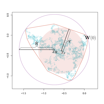
Figure 1. The convex hull $\mathrm{H}$ together with the smallest circle in which it is contained, and the largest circle contained in $\mathrm{H}$. The center of the smallest circle which contains $\mathrm{H}$ is denoted by $x_{\mathsf{R}}$, and the corresponding circumradius is $\mathsf{R}$. The center of the largest circle contained in $\mathrm{H}$ (Chebyshev’s center) is denoted by $x_{\mathsf{r}}$, and the corresponding inradius is $\mathsf{r}$.

To the best of our knowledge, no bounds on the expected value of $\mathsf{R}(t)$ and $\mathsf{r}(t)$ are available in the literature, so one of the contributions of this article is to establish lower and upper bounds for $\mathbb{E}[\mathsf{R}(t)]$ and $\mathbb{E}[\mathsf{r}(t)]$. These bounds are presented in the following propositions, cf. Table 1 for Monte Carlo estimates of $\mathbb{E}[\mathsf{R}]$ and $\mathbb{E}[\mathsf{r}]$. We remark that in light of Brownian scaling, it is enough to obtain bounds only for $t=1$, cf. Proposition 4.1.

We first observe that we can obtain a lower and an upper bound on the expected value of the circumradius directly from the trivial almost sure inequality $4\mathsf{R}\leq\mathsf{P}\leq 2\pi\mathsf{R}$ (the extrema again being realized by a line segment, and a disc), and formula (1). More precisely, this yields

$$0.7978\approx\sqrt{\frac{2}{\pi}}\leq\mathbb{E}[\mathsf{R}]\leq\sqrt{\frac{\pi}{2}}\approx 1.2534.$$

We next improve on both of these bounds.

Proposition 1.2.

In the above notation it holds that

$$0.928\leq\mathbb{E}[\mathsf{R}]\leq\frac{1}{2\pi}\left(\sqrt{8\pi}+\sqrt{\mathbb{E}[\mathsf{P}^{2}]-2\pi^{2}}\right)\approx 1.2028.$$ (10)

To prove the lower bound in (10) we use the obvious fact that $\mathsf{D}\leq 2\mathsf{R}$ and combine it with (8). For the upper bound in (10) we apply a Bonnesen–type inequality from [18, Equation 20] that involves circumradius, perimeter, and area, and we combine it with Jensen’s inequality and the known results from (1), (3) and (4). For a detailed proof see Section 3.

When it comes to inradius, we obtain the following bounds.

Proposition 1.3.

In the above notation it holds that

$$0.3930\approx\frac{1}{2\pi}\left(\sqrt{8\pi}-\sqrt{\mathbb{E}\left[\mathsf{P}^{2}\right]-2\pi^{2}}\right)\leq\mathbb{E}[\mathsf{r}]\leq\frac{\sqrt{2}}{2}\approx 0.7072.$$ (11)

To prove the lower bound in (11) we again apply a Bonnesen–type inequality. This one involves inradius, perimeter, and area (see [18, Equation 15]), and we combine it with Jensen’s inequality and the known results from (1), (3) and (4). For the upper bound in (11) we use the obvious fact that $\mathsf{A}\geq\pi\mathsf{r}^{2}$ and combine it with Jensen’s inequality. For a detailed proof see Section 3.

In the following proposition, we find an alternative lower bound for $\mathbb{E}[\mathsf{r}]$ by considering a particular triangle, embedded in the path of the Brownian motion, whose inradius is amenable to estimation. While this lower bound is somewhat worse than the one in (11), it has the advantage of being constructive. For details see Section 3.

Proposition 1.4.

In the above notation it holds that

$$\mathbb{E}[\mathsf{r}]\geq\frac{\sqrt{\pi}}{8+4\sqrt{2}}\approx 0.1297.$$

Bounds on expected times to reach a given size

There is a question which arises naturally in the present context, namely how much time does it take for planar Brownian motion to span a convex hull of a given size? This question can be investigated in terms of the basic geometric quantities such as perimeter, area, diameter, circumradius and inradius, and it results in establishing bounds on the expectation of the corresponding inverse processes. The main aim of this article is to find such bounds and thus to give (at least a partial) answer to the question posed above.

We consider the inverse processes $\Theta^{\mathsf{P}}(y)$, $\Theta^{\mathsf{A}}(y)$, $\Theta^{\mathsf{D}}(y)$, $\Theta^{\mathsf{R}}(y)$ and $\Theta^{\mathsf{r}}(y)$ that correspond to the processes $\mathsf{P}(t)$, $\mathsf{A}(t)$, $\mathsf{D}(t)$, $\mathsf{R}(t)$ and $\mathsf{r}(t)$, respectively. We start by presenting bounds on the inverse perimeter process. We remark that in view of the scaling properties of the studied inverse processes (see Proposition 4.1), it is enough to give bounds only in the case when $y=1$.

Proposition 1.5.

In the above notation it holds that

$$0.0397\approx\frac{1}{8\pi}\leq\mathbb{E}\left[\Theta^{\mathsf{P}}\right]\leq\frac{1}{2\pi^{2}}\approx 0.0507.$$ (12)

The lower bound in (12) follows from the corresponding equivalence in law from Proposition 4.1 combined with Jensen’s inequality and (1). The upper bound also rests on Jensen’s inequality, but this time it is combined with Cauchy’s surface area formula (2). For more details we refer to Section 4.1.

Bounds on the expectation of the inverse area process are presented below.

Proposition 1.6.

In the above notation it holds that

$$0.6366\approx\frac{2}{\pi}\leq\mathbb{E}\left[\Theta^{\mathsf{A}}\right]\leq 4\sqrt{\mathbb{E}\Big{[}\min\big{\{}\Theta^{R_{1}},\,\Theta^{R_{2}}\big{\}}\Big{]}}\approx 2.3548,$$ (13)

where $R_{1}$ and $R_{2}$ are two independent range processes defined in (7).

The lower bound in (13) follows from the corresponding equivalence in law from Proposition 4.1 combined with Jensen’s inequality and (4). To find the upper bound in (13), we perform a two-stage geometric procedure which results in squeezing a certain triangle into $\mathrm{H}(t)$, and enables us to bound the expected value of $\Theta^{\mathsf{A}}$ in terms of $\mathbb{E}\big{[}\min\big{\{}\Theta^{R_{1}},\,\Theta^{R_{2}}\big{\}}\big{]}$. For details we refer to Section 4.1.

The expected value of the minimum of two independent range times features in several of our estimates, including (13). In the following lemma we derive an integral expression for this quantity. Despite its relatively simple form, the definite integral seems difficult to evaluate explicitly, though it can be evaluated numerically to arbitrary precision using software such as Mathematica.

Lemma 1.7.

It holds that

$$\mathbb{E}\big{[}\min\big{\{}\Theta^{R_{1}},\,\Theta^{R_{2}}\big{\}}\big{]}=\frac{1}{2}-\frac{2}{\pi}\int_{0}^{\infty}\left(1-\frac{4}{(\cos t+\cosh t)^{2}}\right)\frac{1}{t^{3}}\mathop{\mathrm{d}t}\approx 0.346554.$$

For the proof of Lemma 1.7, we find a closed-form formula for the characteristic function of the random variable $\Theta^{R_{1}}-\Theta^{R_{2}}$ which is valid on the whole positive real semi-axis; see Section 2 for details.

Bounds on the expectation of the inverse diameter process are displayed below.

Proposition 1.8.

In the above notation it holds that

$$0.1803\approx\frac{1}{8\log 2}\leq\mathbb{E}\left[\Theta^{\mathsf{D}}\right]\leq\mathbb{E}\big{[}\min\big{\{}\Theta^{R_{1}},\Theta^{R_{2}}\big{\}}\big{]}\approx 0.3466,$$ (14)

where $R_{1}$ and $R_{2}$ are two independent range processes defined in (7).

The lower bound in (14) follows from the corresponding equivalence in law from Proposition 4.1 combined with Jensen’s inequality and the upper bound from (5). The upper bound in (14) follows from the obvious fact that as soon as one of the two coordinates of $\mathbf{W}(t)$ attains range $1$, then the diameter of $\mathrm{H}(t)$ must be at least $1$. For more details we refer to Section 4.1.

Bounds on the expectation of the inverse circumradius process are presented below.

Proposition 1.9.

In the above notation it holds that

$$\mathbb{E}\left[\Theta^{\mathsf{R}}\right] \geq\mathbb{E}[\min\{\Theta^{R_{1}}(\sqrt{2}),\,\Theta^{R_{2}}(\sqrt{2})\}]\approx 0.6931\text{ and}$$ (15)

$$\mathbb{E}\left[\Theta^{\mathsf{R}}\right] \leq\mathbb{E}[\min\{\Theta^{R_{1}}(2),\,\Theta^{R_{2}}(2)\}]\approx 1.3863,$$

where $R_{1}$ and $R_{2}$ are two independent range processes defined at (7).

The lower bound in (15) follows from the fact that when one of the coordinates of $\mathbf{W}(t)$ first attains range $\sqrt{2}$, the whole path is still contained in a square with side length $\sqrt{2}$. Hence, the circumradius of the convex hull of the path is smaller than or equal to half of the diagonal of such square. On the other hand, as soon as one of the two independent range processes hits value $2$, the circumradius must be at least $1$. For a detailed proof see Section 4.1.

The most challenging task of this article is to obtain bounds (especially an upper bound) on the expected time needed for the inradius process to attain value $1$.

Proposition 1.10.

In the above notation it holds that

$$2\leq\mathbb{E}\left[\Theta^{\mathsf{r}}\right]\leq 83.4.$$ (16)

While the upper bound in (16) seems far from being sharp, cf. Table 1, we find the method that allowed us to obtain this upper bound very interesting nevertheless. We now embark on a brief discussion of our approach. To prove the lower bound in (16), we apply the isoperimetric inequality combined with the corresponding equivalence in law from Proposition 4.1 (v) and the lower bound from (13). For the upper bound, we employ a two-stage construction similar to that of Proposition 1.6. More precisely, we first wait until one of the coordinates of $\mathbf{W}$ attains a given range. This waiting time is distributed like the random variable $\min\{\Theta^{R_{1}}(a),\,\Theta^{R_{2}}(a)\}$ for a parameter $a>0$. At this time the convex hull will contain a line segment of length at least $a$ with the Brownian motion being located at one of the endpoints of this line segment. To explain the second stage of our construction, we recall the definition of a radial slit plane. For $n\in\mathbb{N}$, we denote by $\mathcal{S}_{n}$ the complex plane with $n$ equally spaced radial slits emanating from the unit disk. More precisely,

$$\mathcal{S}_{n}=\mathbb{C}\setminus\{z\in\mathbb{C}:|z|\geq 1~{}\mathrm{and}\,\operatorname{Arg}z^{n}=0\}.$$ (17)

In the second stage of the construction, we wait until $\mathbf{W}$ exits a radial slit plane $r\mathcal{S}_{6}$ (i.e. with $6$ slits that reach to within distance $r$ of the origin), where $r>0$ is another parameter. After this step is completed, the inradius of $\mathrm{H}$ will be bigger than some explicit function $\varrho(a,r)>0$, which is equal to the inradius of a certain triangle that is contained in the convex hull. This will result in the following bound

$$\mathbb{E}\left[\Theta^{\mathsf{r}}(\varrho(a,r))\right]\leq\mathbb{E}\left[\min\big{\{}\Theta^{R_{1}}(a),\,\Theta^{R_{2}}(a)\big{\}}\right]+\mathbb{E}\left[\tau_{r\mathcal{S}_{6}}\right],$$ (18)

where $\tau_{r\mathcal{S}_{n}}$ stands for the exit time of $\mathbf{W}$ from $r\mathcal{S}_{n}$. Successfully exploiting estimate (18) requires the precise value of $\mathbb{E}[\tau_{\mathcal{S}_{n}}]$, and this result, which is itself a new contribution, is displayed in the following theorem (its proof is given in Section 4.2).

Theorem 1.11.

In the above notation it holds that

$$\mathbb{E}\left[\tau_{\mathcal{S}_{n}}\right]=\begin{cases}\infty&n\leq 4\\ \displaystyle\frac{\Gamma\left(\frac{1}{2}-\frac{2}{n}\right)}{2\sqrt{\pi}\,\Gamma\left(1-\frac{2}{n}\right)}&n\geq 5.\end{cases}$$

Finally, estimate (18) can be combined with Theorem 1.11 and Lemma 1.7, and accompanied by an optimization procedure along parameters $a$ and $r$ to yield the desired upper bound in (16). For a detailed proof see Section 4.3.

Remark 1.12.

In the two-stage constructions used to prove Propositions 1.6 and 1.10, we could have alternatively constructed the first line segment of length at least $a$ by waiting until $\mathbf{W}$ exits from a ball of radius $a$. However, this turns out to result in a worse estimate since the expected time until $\mathbf{W}$ exits from a ball of radius $a$ (starting from the center of the ball) is $a^{2}/2$, which is bigger than the expected value of the random variable $\min\{\Theta^{R_{1}}(a),\,\Theta^{R_{2}}(a)\}$; see (22) and Lemma 1.7.

The rest of the article is organized as follows. In Section 2 we study the minimum of two independent inverse range processes. In Section 3 we present bounds on the expectation of the circumradius and the inradius of $\mathrm{H}$. In Section 4 we give proofs of bounds for all inverse processes. Finally, in Section 5 we discuss some technical details related to simulations and numerical integration.

2. Minimum of two Inverse Range processes

This section is devoted to the proof of Lemma 1.7. Before we embark on the proof, we start with some preparation which concerns a one-dimensional range process related to a Brownian motion. For this reason we set $W(t)$ to be a one-dimensional Brownian motion started at $0$ and let $R(t)$ be its range process defined as

$$R(t)=\sup_{0\leq s\leq t}W(s)-\inf_{0\leq s\leq t}W(s),\quad t\geq 0,$$

cf. (7). We remark that the convex hull spanned by a path of $W(t)$ up to time $t$ is nothing but the segment $[\inf_{0\leq s\leq t}W(s),\sup_{0\leq s\leq t}W(s)]$ whose length is equal to $R(t)$. The right-continuous inverse range process $\{\Theta(y):\,y\geq 0\}$ is defined as the exit time

$$\Theta(y)=\inf\{t\geq 0:R(t)>y\}.$$

It is known that $\Theta(y)$ has independent increments. The processes $R(t)$ and $\Theta(y)$ are both well studied and their marginal laws are known explicitly. By [8, Equation 3.6], the density of $R(1)$ is given by equation (9). Before we present a formula for the density of the random variable $\Theta(1)$, we first recall that its Laplace transform is given by, see [11],

$$\mathbb{E}\left[e^{-\lambda\Theta(y)}\right]=\sech^{2}\left(y\sqrt{\lambda/2}\right),\quad\lambda\geq 0.$$ (19)

Further, the authors of [2] studied the following random variable

$$C_{2}=\frac{2}{\pi^{2}}\sum_{n=1}^{\infty}\frac{\Gamma_{2,n}}{(n-\frac{1}{2})^{2}},$$

where $\Gamma_{2,n}$ are independent random variables with distribution $\mathrm{Gamma}(2,1)$. According to [2, Eq. (1.8)], the random variable $C_{2}$ has the Laplace transform

$$\mathbb{E}\left[e^{-\lambda C_{2}}\right]=\frac{1}{\cosh^{2}\big{(}\sqrt{2\lambda}\big{)}},\quad\lambda\geq 0.$$ (20)

In view of the hyperbolic identity $\sech x=1/\cosh x$, and by comparing (19) and (20), we conclude that $\Theta(1)\stackrel{{\scriptstyle d}}{{=}}4^{-1}C_{2}$. Thus, we can find the density of $\Theta(1)$ in [2, Table 1] and it is given by

$$f_{\Theta}(t)=4\sum_{n=0}^{\infty}\left((2n+1)^{2}\pi^{2}t-1\right)\exp\left(-\frac{(2n+1)^{2}\pi^{2}}{2}t\right),\quad t>0.$$ (21)

Interestingly, a comparable expression for the Laplace transform of the range seems difficult to compute from (9) and appears to be absent from the literature. The scaling property of Brownian motion evidently implies the following equivalences in law

$$R(t)\stackrel{{\scriptstyle d}}{{=}}\sqrt{t}R(1),~{}~{}\Theta(y)\stackrel{{\scriptstyle d}}{{=}}y^{2}\Theta(1),~{}~{}\Theta(y)\stackrel{{\scriptstyle d}}{{=}}\frac{y^{3}}{R^{2}(y)}.$$ (22)

See Proposition 4.1 for other similar equivalences in law.

We now proceed to the proof of Lemma 1.7.

Proof of Lemma 1.7.

We start by finding a formula for the characteristic function of the random variable $\Theta(1)-\widetilde{\Theta}(1)$ that is valid for any nonnegative real argument. Here, $\widetilde{\Theta}(1)$ is an independent copy of $\Theta(1)$. In the rest of the proof we simply write $\Theta$ for $\Theta(1)$, and $\widetilde{\Theta}$ for $\widetilde{\Theta}(1)$. From (21), we immediately see that the exponential rate of decay of the right-tail of the density of $\Theta$ is $\frac{\pi^{2}}{2}$. Hence, the Laplace transform $z\mapsto\mathbb{E}[e^{-z\Theta}]$ exists and is analytic in the right half-plane $\mathbb{H}=\{z\in\mathbb{C}:\operatorname*{Re}z>-\frac{\pi^{2}}{2}\}$; see e.g. [27, Chapter II]. Moreover, $\sech^{2}(\sqrt{z/2})$ is a meromorphic function with no poles in $\mathbb{H}$. This follows from the fact that $\cosh z$ is an entire function whose Taylor expansion contains only even powers and whose zeros occur at the points $i\pi(2k+1)/2$, $k\in\mathbb{Z}$. Therefore, formula (19) for the Laplace transform with $y=1$ is actually valid for all $\lambda\in\mathbb{H}$.

For $s\geq 0$, we use the identity $\cosh z=\cos iz$ which yields

$$\mathbb{E}\left[e^{i4s(\Theta-\widetilde{\Theta})}\right] =\mathbb{E}\left[e^{i4s\Theta}\right]\mathbb{E}\left[e^{-i4s\Theta}\right]$$

$$=\sech^{2}\left((1-i)\sqrt{s}\right)\sech^{2}\left((1+i)\sqrt{s}\right)$$

$$=\frac{1}{\cos^{2}\left((i+1)\sqrt{s}\right)}\frac{1}{\cos^{2}\left((i-1)\sqrt{s}\right)}.$$ (23)

The identity $\cos(x+iy)=\cos x\cosh y-i\sin x\sinh y$ for $x,y\in\mathbb{R}$ can be used to express the right-hand side of (23) as

$$\frac{1}{(\cos\sqrt{s}\cosh\sqrt{s}-i\sin\sqrt{s}\sinh\sqrt{s})^{2}}\frac{1}{(\cos\sqrt{s}\cosh\sqrt{s}+i\sin\sqrt{s}\sinh\sqrt{s})^{2}}$$

$$=\frac{1}{(\cos^{2}\sqrt{s}\cosh^{2}\sqrt{s}+\sin^{2}\sqrt{s}\sinh^{2}\sqrt{s})^{2}}$$

$$=\frac{1}{(\cosh^{2}\sqrt{s}-\sin^{2}\sqrt{s})^{2}}.$$ (24)

The last equality follows from expanding $\cos^{2}$ and then collapsing the resulting factor $\sinh^{2}-\cosh^{2}$ using well-known identities. Further, combining (23) and (24) along with the double-angle identities for $\cos$ and $\cosh$ leads to the formula

$$\mathbb{E}\left[e^{is(\Theta-\widetilde{\Theta})}\right]=\frac{4}{(\cos\sqrt{s}+\cosh\sqrt{s})^{2}},\quad s\geq 0.$$ (25)

The last step of the proof is to use the elementary identity

$$\min\{x,y\}=\frac{1}{2}(x+y-|x-y|),\quad x,y\in\mathbb{R}$$

and an integral formula for the absolute moments of a random variable in terms of its characteristic function; see [4, Lemma 1]. In view of (25) we obtain

$$\mathbb{E}\left[\min\left\{\Theta,\widetilde{\Theta}\right\}\right] =\mathbb{E}[\Theta]-\frac{1}{2}\mathbb{E}\left[\left|\Theta-\widetilde{\Theta}\right|\right]$$

$$=\frac{1}{2}-\frac{1}{\pi}\int_{0}^{\infty}\left(1-\frac{4}{(\cos\sqrt{s}+\cosh\sqrt{s})^{2}}\right)\frac{1}{s^{2}}\mathop{\mathrm{d}s}$$

$$=\frac{1}{2}-\frac{2}{\pi}\int_{0}^{\infty}\left(1-\frac{4}{(\cos t+\cosh t)^{2}}\right)\frac{1}{t^{3}}\mathop{\mathrm{d}t},$$

where the last equality follows from the change of variables $\sqrt{s}=t$. ∎

Remark 2.1.

We note that an alternative expression for the expected value from Lemma 1.7 can be derived from the density (21). However, the resulting infinite series turns out to be rather unwieldy, so we omit it.

3. Bounds on the expectation of circumradius and inradius

In this section we give detailed proofs for our bounds on the expected values of the circumradius $\mathsf{R}$ and inradius $\mathsf{r}$ that are included in Proposition 1.2, Proposition 1.3 and Proposition 1.4.

Proof of Proposition 1.2.

To prove the lower bound, we just employ a trivial observation that $\mathsf{D}\leq 2\mathsf{R}$, together with (8). More precisely, we have

$$\mathbb{E}[\mathsf{R}]\geq\frac{1}{2}\mathbb{E}[\mathsf{D}]\geq\frac{1.856}{2}=0.928.$$

For the upper bound, we start with the following Bonnesen-type inequality [18, Equation 20] that involves circumradius, perimeter, and area

$$\mathsf{R}\leq\frac{1}{2\pi}\left(\mathsf{P}+\sqrt{\mathsf{P}^{2}-4\pi\mathsf{A}}\right).$$ (26)

Taking expectations while using Jensen’s inequality on the right-hand side along with (1), (3), and (4) leads to

$$\mathbb{E}[\mathsf{R}] \leq\frac{1}{2\pi}\left(\mathbb{E}[\mathsf{P}]+\sqrt{\mathbb{E}\left[\mathsf{P}^{2}\right]-4\pi\mathbb{E}[\mathsf{A}]}\right)$$

$$=\frac{1}{2\pi}\left(\sqrt{8\pi}+\sqrt{\mathbb{E}\left[\mathsf{P}^{2}\right]-2\pi^{2}}\right)\approx 1.2027.$$

∎

Remark 3.1.

Using our simulations, we can estimate the expected value of the right-hand side of (26), that is

$$\frac{1}{2\pi}\mathbb{E}\left[\left(\mathsf{P}+\sqrt{\mathsf{P}^{2}-4\pi\mathsf{A}}\right)\right],$$

without relying on Jensen’s inequality. Monte Carlo estimation of this quantity is $1.176$ which suggests that we did not lose too much when applying Jensen’s inequality.

Proof of Proposition 1.3.

To prove the lower bound, we use another Bonnesen-type inequality [18, Equation 15]. This one involves inradius, perimeter, and area, and it takes the form

$$\mathsf{r}\geq\frac{1}{2\pi}\left(\mathsf{P}-\sqrt{\mathsf{P}^{2}-4\pi\mathsf{A}}\right).$$ (27)

Taking expectations while using Jensen’s inequality on the right-hand side along with (1), (3), and (4) leads to

$$\mathbb{E}[\mathsf{r}] \geq\frac{1}{2\pi}\left(\mathbb{E}[\mathsf{P}]-\sqrt{\mathbb{E}\left[\mathsf{P}^{2}\right]-4\pi\mathbb{E}[\mathsf{A}]}\right)$$

$$=\frac{1}{2\pi}\left(\sqrt{8\pi}-\sqrt{\mathbb{E}\left[\mathsf{P}^{2}\right]-2\pi^{2}}\right)\approx 0.39305.$$

For the upper bound, we start from the obvious inequality $\mathsf{A}\geq\pi\mathsf{r}^{2}$ which yields $\mathsf{r}\leq\sqrt{\mathsf{A}/\pi}$. By using Jensen’s inequality and (4) we arrive at

$$\mathbb{E}\left[\mathsf{r}\right]\leq\frac{1}{\sqrt{\pi}}\mathbb{E}\left[\sqrt{\mathsf{A}}\right]\leq\frac{1}{\sqrt{\pi}}\sqrt{\mathbb{E}[\mathsf{A}]}=\frac{\sqrt{2}}{2}$$

and the proof is complete. ∎

Remark 3.2.

Using our simulations, we can estimate the expected value of the right-hand side of (27), that is

$$\frac{1}{2\pi}\mathbb{E}\left[\left(\mathsf{P}-\sqrt{\mathsf{P}^{2}-4\pi\mathsf{A}}\right)\right],$$

without relying on Jensen’s inequality. Monte Carlo estimation of this expectation is $0.418$ which suggests that we do not lose too much with Jensen’s inequality. We also estimated the value of $\mathbb{E}[\sqrt{\mathsf{A}/\pi}]$, and got $0.696$, which is only a bit smaller than $\sqrt{2}/2$.

Proof of Proposition 1.4.

We estimate the inradius of the triangle with vertices $\mathbf{W}(0)$, $\mathbf{W}(1/2)$, and $\mathbf{W}(1)$ that is contained in the convex hull $\mathrm{H}$; see Figure 2.

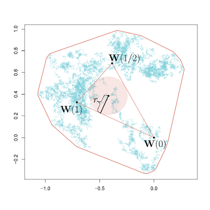
Figure 2. The triangle with vertices $\mathbf{W}(0)$, $\mathbf{W}(1/2)$, and $\mathbf{W}(1)$ contained in $\mathrm{H}$. The inradius of the triangle is denoted with $r$.

More generally, we could choose the intermediate point at some $t\in(0,1)$ instead of at $1/2$, however, $1/2$ apparently provides the best estimate. Let us denote the lengths of the line segments $\overline{\mathbf{W}(0)\mathbf{W}(1/2)}$, $\overline{\mathbf{W}(1/2)\mathbf{W}(1)}$, and $\overline{\mathbf{W}(0)\mathbf{W}(1)}$ by $A$, $B$, and $C$, respectively. Further, we denote the angle $\angle(\mathbf{W}(0),\mathbf{W}(1/2),\mathbf{W}(1))$ by $\theta$. Using the fact that the inradius of a triangle is the quotient of its area and semiperimeter, we obtain

$$\mathbb{E}[\mathsf{r}]\geq\mathbb{E}\left[\frac{AB\sin\theta}{A+B+C}\right].$$ (28)

Applying the reverse Hölder inequality to the right-hand side of (28) results in

$$\mathbb{E}[\mathsf{r}]\geq\frac{\mathbb{E}\left[\sqrt{AB\sin\theta}\right]^{2}}{\mathbb{E}[A+B+C]}.$$ (29)

The rotational invariance and Markov property of planar Brownian motion imply that $A$, $B$, and $\theta$ are mutually independent, that $A$ and $B$ have the same law, and that $\theta$ is uniform on $(0,\pi)$. Moreover, Brownian scaling implies that $C$ has the same law as $\sqrt{2}A$. Since the radial displacement of planar Brownian motion is a $2$-dimensional Bessel process (see [19, Chapter XI.1]), we have

$$\mathbb{P}(A\in\mathop{\mathrm{d}x})=2xe^{-x^{2}}\mathop{\mathrm{d}x}.$$

These facts imply

$$\mathbb{E}[A+B+C] =\left(2+\sqrt{2}\right)\mathbb{E}[A]=2\left(2+\sqrt{2}\right)\int_{0}^{\infty}x^{2}e^{-x^{2}}\mathop{\mathrm{d}x}$$

$$=\left(2+\sqrt{2}\right)\frac{\sqrt{\pi}}{2}$$ (30)

and

$$\mathbb{E}\left[\sqrt{AB\sin\theta}\right] =\mathbb{E}\left[\sqrt{A}\right]^{2}\mathbb{E}\left[\sqrt{\sin\theta}\right]$$

$$=4\left(\int_{0}^{\infty}x^{\frac{3}{2}}e^{-x^{2}}\mathop{\mathrm{d}x}\right)^{2}\int_{0}^{\pi}\frac{\sqrt{\sin u}}{\pi}\mathop{\mathrm{d}u}$$ (31)

$$=\Gamma\left(\frac{5}{4}\right)^{2}\frac{2\sqrt{2}\,\Gamma\left(\frac{3}{4}\right)^{2}}{\pi^{\frac{3}{2}}}=\sqrt{\frac{\pi}{8}}.$$ (32)

The second integral appearing in (31) can be evaluated using [10, Identity 3.621.1], while the second equality in (32) follows from the Legendre duplication formula. Substituting (30) and (32) into (29) proves the lower bound. ∎

Remark 3.3.

Note that using the law of cosines to eliminate $C$ from (28) and then numerically computing that expectation via the product density of $(A,B,\theta)$ yields a lower bound of approximately $0.1456$, so we do not lose too much using the reverse Hölder inequality.

4. Bounds on the expectations of the inverse processes

In this section we provide proofs of the bounds for inverse processes presented in the introduction. We start with an auxiliary result which concerns scaling properties and equalities in law for the processes $\mathsf{P}(t)$, $\mathsf{A}(t)$, $\mathsf{D}(t)$, $\mathsf{R}(t)$, $\mathsf{r}(t)$ and their inverse processes.

Proposition 4.1.

For all $t\geq 0$ and $y>0$, the following equivalences in law hold true.

1. $\displaystyle\mathsf{P}(t)\stackrel{{\scriptstyle d}}{{=}}\sqrt{t}\mathsf{P}(1),~{}~{}\Theta^{\mathsf{P}}(y)\stackrel{{\scriptstyle d}}{{=}}y^{2}\Theta^{\mathsf{P}}(1),~{}~{}\Theta^{\mathsf{P}}(y)\stackrel{{\scriptstyle d}}{{=}}\frac{y^{3}}{\mathsf{P}^{2}(y)}$;

2. $\displaystyle\mathsf{A}(t)\stackrel{{\scriptstyle d}}{{=}}t\,\mathsf{A}(1),~{}~{}\Theta^{\mathsf{A}}(y)\stackrel{{\scriptstyle d}}{{=}}y\,\Theta^{\mathsf{A}}(1),~{}~{}\Theta^{\mathsf{A}}(y)\stackrel{{\scriptstyle d}}{{=}}\frac{y^{2}}{\mathsf{A}(y)}$;

3. $\displaystyle\mathsf{D}(t)\stackrel{{\scriptstyle d}}{{=}}\sqrt{t}\mathsf{D}(1),~{}~{}\Theta^{\mathsf{D}}(y)\stackrel{{\scriptstyle d}}{{=}}y^{2}\Theta^{\mathsf{D}}(1),~{}~{}\Theta^{\mathsf{D}}(y)\stackrel{{\scriptstyle d}}{{=}}\frac{y^{3}}{\mathsf{D}^{2}(y)}$;

4. $\displaystyle\mathsf{R}(t)\stackrel{{\scriptstyle d}}{{=}}\sqrt{t}\mathsf{R}(1),~{}~{}\Theta^{\mathsf{R}}(y)\stackrel{{\scriptstyle d}}{{=}}y^{2}\Theta^{\mathsf{R}}(1),~{}~{}\Theta^{\mathsf{R}}(y)\stackrel{{\scriptstyle d}}{{=}}\frac{y^{3}}{\mathsf{R}^{2}(y)}$;

5. $\displaystyle\mathsf{r}(t)\stackrel{{\scriptstyle d}}{{=}}\sqrt{t}\mathsf{r}(1),~{}~{}\Theta^{\mathsf{r}}(y)\stackrel{{\scriptstyle d}}{{=}}y^{2}\Theta^{\mathsf{r}}(1),~{}~{}\Theta^{\mathsf{r}}(y)\stackrel{{\scriptstyle d}}{{=}}\frac{y^{3}}{\mathsf{r}^{2}(y)}$.

Proof.

We start with a proof for the process $\mathsf{A}(t)$. The scaling property of Brownian motion implies that

$$\mathrm{H}(t)=\mathrm{conv}\{\mathbf{W}(s):0\leq s\leq t\}\stackrel{{\scriptstyle d}}{{=}}\sqrt{t}\,\mathrm{conv}\{\mathbf{W}(s):0\leq s\leq 1\}=\sqrt{t}\,\mathrm{H}(1).$$ (33)

Hence $\mathsf{A}(t)\stackrel{{\scriptstyle d}}{{=}}\mathrm{Area}\left(\sqrt{t}\,\mathrm{hull}\{\mathbf{W}(s):0\leq s\leq 1\}\right)=t\,\mathsf{A}(1)$. Similarly, for any $\lambda>0$ we have

$$\mathsf{A}(\lambda t) =\mathrm{Area}(\mathrm{conv}\{\mathbf{W}(s):0\leq s\leq\lambda t\})=\mathrm{Area}(\mathrm{conv}\{\mathbf{W}(\lambda s):0\leq s\leq t\})$$

$$\stackrel{{\scriptstyle d}}{{=}}\mathrm{Area}(\mathrm{conv}\{\sqrt{\lambda}\mathbf{W}(s):0\leq s\leq t\})=\lambda\mathsf{A}(t).$$ (34)

This implies

$$\mathbb{P}(\Theta^{\mathsf{A}}(y)>t) =\mathbb{P}(\mathsf{A}(t)<y)=\mathbb{P}\left(\mathsf{A}\left(y\cdot\frac{t}{y}\right)<y\right)=\mathbb{P}(y\,\mathsf{A}(t/y)<y)$$

$$=\mathbb{P}(\mathsf{A}(t/y)<1)=\mathbb{P}(\Theta^{\mathsf{A}}(1)>t/y)=\mathbb{P}(y\,\Theta^{\mathsf{A}}(1)>t).$$

Finally, we have

$$\mathbb{P}\left(\Theta^{\mathsf{A}}(y)>t\right)=\mathbb{P}\left(\mathsf{A}(t)<y\right)=\mathbb{P}\left(\mathsf{A}\left(y\cdot\frac{t}{y}\right)<y\right)=\mathbb{P}\left(\frac{t}{y}\mathsf{A}(y)<y\right)=\mathbb{P}\left(\frac{y^{2}}{\mathsf{A}(y)}>t\right).$$

To prove the first equality in law in (i), (iii), (iv) and (v) we can again use (33) together with the fact that the functionals in question are homogeneous of order one. For completeness, we provide some more details.

For the proof of the first equality in law in (i) we use (33), which evidently yields $\mathsf{P}(\lambda t)\stackrel{{\scriptstyle d}}{{=}}\sqrt{\lambda}\mathsf{P}(t)$, for any $\lambda>0$. This further implies

$$\mathbb{P}(\Theta^{\mathsf{P}}(y)>t) =\mathbb{P}(\mathsf{P}(t)<y)=\mathbb{P}\left(\frac{1}{y}\mathsf{P}(t)<1\right)=\mathbb{P}(\mathsf{P}(t/y^{2})<1)$$

$$=\mathbb{P}\left(\Theta^{\mathsf{P}}(1)>\frac{t}{y^{2}}\right)=\mathbb{P}(y^{2}\Theta^{\mathsf{P}}(1)>t).$$

Similarly, we have

$$\mathbb{P}(\Theta^{\mathsf{P}}(y)>t) =\mathbb{P}\left(\frac{1}{y}\mathsf{P}(t)<1\right)=\mathbb{P}\left(\frac{1}{y}\mathsf{P}\left(y\cdot\frac{t}{y}\right)<1\right)$$

$$=\mathbb{P}\left(\sqrt{\frac{t}{y^{3}}}\mathsf{P}(y)<1\right)=\mathbb{P}\left(\frac{y^{3}}{\mathsf{P}^{2}(y)}>t\right).$$

To show the first equality in law in (iii) we simply use $\mathsf{D}(t)=\sup_{x,y\in\mathrm{H}(t)}\norm{x-y}$ together with the Brownian scaling, where $\norm{x}$ stands for Euclidean norm of vector $x$. The remaining two equivalences can be proved analogously as for the process $\mathsf{P}(t)$.

We now prove (iv). Let $B(x,\rho)$ denote the closed ball in $\mathbb{R}^{2}$ centered at $x$ and of radius $\rho$. We have

$$\mathsf{R}(t) =\inf\{\rho>0:(\exists\,x\in\mathbb{R}^{2})\,\mathrm{H}(t)\subset B(x,\rho)\}$$

$$\stackrel{{\scriptstyle d}}{{=}}\inf\{\rho>0:(\exists\,x\in\mathbb{R}^{2})\,\sqrt{t}\,\mathrm{H}(1)\subset B(x,\rho)\}$$

$$=\inf\{\rho>0:(\exists\,x\in\mathbb{R}^{2})\,\mathrm{H}(1)\subset B(x,t^{-1/2}\rho)\}=\sqrt{t}\,\mathsf{R}(1).$$

We can similarly show that $\mathsf{R}(\lambda t)\stackrel{{\scriptstyle d}}{{=}}\sqrt{\lambda}\,\mathsf{R}(t)$, for any $\lambda>0$, which implies the other two equivalences from (iv) similarly to the case of (i).

Finally, we have

$$\mathsf{r}(t) =\sup\{\rho>0:(\exists\,x\in\mathrm{H}(t))\,B(x,\rho)\subset\mathrm{H}(t)\}$$

$$\stackrel{{\scriptstyle d}}{{=}}\sup\{\rho>0:(\exists\,x\in\sqrt{t}\,\mathrm{H}(1))\,B(x,\rho)\subset\sqrt{t}\,\mathrm{H}(1)\}$$

$$=\sup\{\rho>0:(\exists\,x\in\mathrm{H}(1))\,B(\sqrt{t}\,x,\rho)\subset\sqrt{t}\,\mathrm{H}(1)\}$$

$$=\sup\{\rho>0:(\exists\,x\in\mathrm{H}(1))\,B(x,t^{-1/2}\rho)\subset\mathrm{H}(1)\}=\sqrt{t}\,\mathsf{r}(1).$$

We can similarly show that $\mathsf{r}(\lambda t)\stackrel{{\scriptstyle d}}{{=}}\sqrt{\lambda}\,\mathsf{r}(t)$, for any $\lambda>0$. As in the (iv) case, this implies the other two equivalences from (v) and the proof is complete.

∎

4.1. Bounds on inverse perimeter, area, diameter and circumradius

We are now ready to prove the series of propositions for inverse processes.

Proof of Proposition 1.5.

For the lower bound we simply have

$$\mathbb{E}[\Theta^{\mathsf{P}}]=\mathbb{E}\left[\frac{1}{\mathsf{P}^{2}}\right]\geq\frac{1}{\left(\mathbb{E}[\mathsf{P}]\right)^{2}}=\frac{1}{8\pi},$$

where we used Proposition 4.1 (i), Jensen’s inequality and (1).

The upper bound also requires Jensen’s inequality, but this time it is used in conjunction with Cauchy’s surface area formula. Recalling that formula from (2), we have

$$\mathsf{P}=\frac{1}{2}\int_{-\pi}^{\pi}\underbrace{\sup_{0\leq s\leq 1}\mathbf{W}(s)\cdot\mathbf{e}_{\theta}-\inf_{0\leq s\leq 1}\mathbf{W}(s)\cdot\mathbf{e}_{\theta}}_{\displaystyle w(\theta)}\mathop{\mathrm{d}\theta},$$

where the $\pi$-periodic function $w(\theta)$ is known as the parametrized width (or parametrized range) of the convex hull $\mathrm{H}$. It follows that Cauchy’s surface area formula can be equivalently stated as

$$\mathsf{P}=\int_{0}^{\pi}w(\theta)\mathop{\mathrm{d}\theta}.$$ (35)

By interpreting the following integrals as expected values with respect to the uniform distribution on $(0,\pi)$, we can use Jensen’s inequality to deduce that

$$\frac{1}{\pi}\int_{0}^{\pi}\frac{1}{w^{2}(\theta)}\mathop{\mathrm{d}\theta}\geq\frac{1}{\left(\frac{1}{\pi}\int_{0}^{\pi}w(\theta)\mathop{\mathrm{d}\theta}\right)^{2}}.$$

In particular, now Cauchy’s surface area formula (35) implies that

$$\frac{1}{\mathsf{P}^{2}}\leq\frac{1}{\pi^{3}}\int_{0}^{\pi}\frac{1}{w^{2}(\theta)}\mathop{\mathrm{d}\theta}.$$ (36)

By rotational invariance of Brownian motion, the law of $w(\theta)$ does not depend on $\theta$. Hence we can combine (36) with Proposition 4.1 (i) and apply Tonelli’s theorem to deduce that

$$\mathbb{E}\left[\Theta^{\mathsf{P}}\right]=\mathbb{E}\left[\frac{1}{\mathsf{P}^{2}}\right]\leq\frac{1}{\pi^{2}}\mathbb{E}\left[\frac{1}{w^{2}(0)}\right].$$

Recall from (7) that $w(0)$ has the same law as the range $R(1)$ of the one-dimensional Brownian motion run up to time $1$. Now it follows from (22) and (19) that

$$\mathbb{E}\left[\Theta^{\mathsf{P}}\right]\leq\frac{1}{\pi^{2}}\mathbb{E}\left[\frac{1}{R^{2}(1)}\right]=\frac{1}{\pi^{2}}\mathbb{E}\left[\Theta(1)\right]=\frac{1}{2\pi^{2}},$$

and the proof is finished. ∎

Proof of Proposition 1.6.

For the lower bound we write

$$\mathbb{E}[\Theta^{\mathsf{A}}]=\mathbb{E}\left[\frac{1}{\mathsf{A}}\right]\geq\frac{1}{\mathbb{E}[\mathsf{A}]}=\frac{2}{\pi},$$

where we applied Proposition 4.1 (ii), Jensen’s inequality and (4).

For the upper bound, we employ a two-stage construction of a stopping time at which the convex hull is guaranteed to contain a triangle of a certain area. First we wait until one of the coordinates of $\mathbf{W}$ has range $a$, where $a$ is a parameter that will be optimized later. This waiting time is distributed like the random variable $\min\{\Theta^{R_{1}}(a),\,\Theta^{R_{2}}(a)\}$ which was investigated in Section 2. Moreover, at this time the convex hull will contain a line segment $\overline{x}$ of length at least $a$ with $\mathbf{W}$ being located at one of the endpoints of $\overline{x}$.

Next, we wait until $\mathbf{W}$ exits an infinite strip of width $2b$ whose axis is collinear with $\overline{x}$. This waiting time $\tau_{b}$ is distributed like the exit time of a one-dimensional Brownian motion from an interval of length $2b$ when starting from the midpoint. It follows that after waiting for both of these events to occur in turn, the convex hull of the planar Brownian motion will contain a triangle with base at least $a$ and height $b$; see Figure 3.

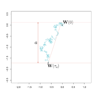
(a) First step.

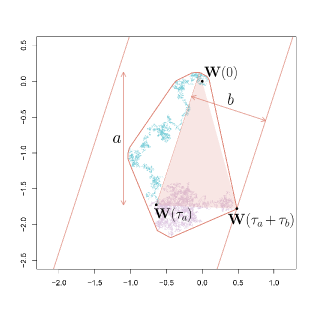
(b) Second step.

Figure 3. In the first step we wait until one of the coordinate range processes hits value $a$. For simplicity, this stopping time is denoted by $\tau_{a}$, that is, $\tau_{a}=\min\{\Theta^{R_{1}}(a),\Theta^{R_{2}}(a)\}$. The trajectory up to this random time is colored blue. In the second step, we wait until $\mathbf{W}$ exits an infinite strip of width $2b$. The trajectory from the time point at which one of the components attained range $a$ till the exit time from the infinite strip of width $2b$ is colored purple. In the end, we are sure that a triangle with base at least $a$, and height $b$ will be contained in the convex hull spanned by the trajectory.

Hence, the area of the convex hull at this time will be at least $ab/2$. This implies that

$$\mathbb{E}\left[\Theta^{\mathsf{A}}(ab/2)\right]\leq\mathbb{E}\left[\min\left\{\Theta^{R_{1}}(a),\,\Theta^{R_{2}}(a)\right\}\right]+\mathbb{E}\left[\tau_{b}\right].$$

Now it follows from (22) and the well-known formula for the expected value of the exit time from an interval for one-dimensional Brownian motion that

$$\mathbb{E}\left[\Theta^{\mathsf{A}}(ab/2)\right]\leq a^{2}\,\mathbb{E}\left[\min\left\{\Theta^{R_{1}},\,\Theta^{R_{2}}\right\}\right]+b^{2}.$$ (37)

Minimizing the right-hand side of (37) under the constraints $ab/2=1$, $a>0$, and $b>0$ results in the desired upper bound

$$\mathbb{E}\left[\Theta^{\mathsf{A}}\right]\leq 4\sqrt{\mathbb{E}\left[\min\left\{\Theta^{R_{1}},\,\Theta^{R_{2}}\right\}\right]}.$$

∎

Proof of Proposition 1.8.

Proposition 4.1 (iii) and Jensen’s inequality together imply that

$$\mathbb{E}\left[\Theta^{\mathsf{D}}\right]\geq\frac{1}{\left(\mathbb{E}\left[\mathsf{D}\right]\right)^{2}}.$$ (38)

Combining (38) with the upper bound from (5) yields the desired lower bound.

The upper bound follows from the fact that as soon as one of the processes $W_{1}(t)$, $W_{2}(t)$ (one of the coordinates of the planar Brownian motion $\mathbf{W}$) attains range $1$, then the diameter of $\mathrm{H}(t)$ is at least $1$. ∎

Proof of Proposition 1.9.

For the lower bound, notice that at the first time when one of the two coordinates of $\mathbf{W}(t)$ attains range $\sqrt{2}$, the other one still has range smaller than or equal to $\sqrt{2}$. This implies that, at this time point, the whole path is contained in a square with side length $\sqrt{2}$. This further implies that the circumscribed circle of that square contains the convex hull of the Brownian path up to that time point. Hence, the smallest circle that contains $\mathrm{H}(t)$ is smaller than or equal to that circle. Since the circumscribed circle of a square with side length $\sqrt{2}$ has radius $1$, we have

$$\mathbb{E}[\Theta^{\mathsf{R}}]\geq\mathbb{E}[\min\{\Theta^{R_{1}}(\sqrt{2}),\,\Theta^{R_{2}}(\sqrt{2})\}]=2\,\mathbb{E}[\min\{\Theta^{R_{1}}(1),\,\Theta^{R_{2}}(1)\}]=0.6931,$$

where we used (22) and Lemma 1.7.

The upper bound is even more simple. As soon as one of the two independent range processes hits value $2$, the convex hull contains a line segment of length at least $2$. Hence at this time point the circumradius must be at least $1$. ∎

4.2. Radial slit plane

Before we can give the proof of Proposition 1.10, we first need to prove Theorem 1.11. We start with a related computational result on the second moment of the radial displacement of the Brownian motion when it exits the radial slit plane $\mathcal{S}_{n}$.

Lemma 4.2.

Let $\mathcal{S}_{n}$ be the radial slit plane defined in (17) and let $\tau_{\mathcal{S}_{n}}$ denote the exit time of $\mathcal{S}_{n}$ by planar the Brownian motion $\mathbf{W}(t)$ started at the origin. Then it holds that

$$\mathbb{E}\left[\norm{\mathbf{W}(\tau_{\mathcal{S}_{n}})}^{2}\right]=\begin{cases}\infty&n\leq 4\\ \displaystyle\frac{\Gamma\left(\frac{1}{2}-\frac{2}{n}\right)}{\sqrt{\pi}\,\Gamma\left(1-\frac{2}{n}\right)}&n\geq 5.\end{cases}$$

Proof of Lemma 4.2.

By [21, Example 2.1], we have

$$\mathbb{P}\Big{(}\norm{\mathbf{W}(\tau_{\mathcal{S}_{n}})}\leq r\Big{)}=\frac{2}{\pi}\arctan\sqrt{r^{n}-1},\quad r\geq 1.$$

Hence,

$$\mathbb{E}\left[\norm{\mathbf{W}(\tau_{\mathcal{S}_{n}})}^{2}\right]=\frac{n}{\pi}\int_{1}^{\infty}\frac{r}{\sqrt{r^{n}-1}}\mathop{\mathrm{d}r}.$$ (39)

Since

$$\frac{r}{\sqrt{r^{n}-1}}=\begin{cases}O(1/\sqrt{r-1}),&\mathrm{as}\ r\searrow 1;\\ O(r^{1-n/2}),&\mathrm{as}\ r\to\infty,\end{cases}$$

it is clear from (39) that $\mathbb{E}\big{[}\norm{\mathbf{W}(\tau_{\mathcal{S}_{n}})}^{2}\big{]}=\infty$ if and only if $n\leq 4$.

We next compute $\mathbb{E}\big{[}\norm{\mathbf{W}(\tau_{\mathcal{S}_{n}})}^{2}\big{]}$ explicitly for $n\geq 5$. For this we apply the change of variables $r=\sec^{2/n}u$ in (39). This results in

$$\mathbb{E}\left[\norm{\mathbf{W}(\tau_{\mathcal{S}_{n}})}^{2}\right] =\frac{n}{\pi}\int_{0}^{\frac{\pi}{2}}\frac{\sec^{\frac{2}{n}}u}{\sqrt{\sec^{2}u-1}}\frac{2\sec^{\frac{2}{n}}u\tan u}{n}\mathop{\mathrm{d}u}$$

$$=\frac{2}{\pi}\int_{0}^{\frac{\pi}{2}}\cos^{-\frac{4}{n}}u\mathop{\mathrm{d}u}$$ (40)

$$=\frac{\Gamma\left(\frac{1}{2}-\frac{2}{n}\right)^{2}}{2^{\frac{4}{n}}\pi\,\Gamma\left(1-\frac{4}{n}\right)}$$

$$=\frac{\Gamma\left(\frac{1}{2}-\frac{2}{n}\right)}{\sqrt{\pi}\,\Gamma\left(1-\frac{2}{n}\right)},\quad n\geq 5.$$ (41)

The integral appearing in (40) can be evaluated using [10, Identity 3.621.1], while the equality in (41) follows from the Legendre duplication formula.

∎

Now we are ready to prove Theorem 1.11.

Proof of Theorem 1.11.

First we show that $\mathbb{E}\left[\tau_{\mathcal{S}_{n}}\right]=\infty$ when $n\leq 4$. Recall that $\mathbf{W}(t)=(W_{1}(t),W_{2}(t))$, where $W_{1}(t)$ and $W_{2}(t)$ are two independent one-dimensional Brownian motions started at zero. Moreover, each process $W_{i}(t)$ is a Brownian motion in the natural filtration of $\mathbf{W}$, with respect to which $\tau_{\mathcal{S}_{n}}$ is a stopping time. In particular, the optional stopping theorem applied to the martingale $W_{1}^{2}(t)+W_{2}^{2}(t)-2t$ implies that for each $j\in\mathbb{N}$ we have

$$\mathbb{E}\left[W_{1}^{2}(\tau_{\mathcal{S}_{n}}\wedge j)+W_{2}^{2}(\tau_{\mathcal{S}_{n}}\wedge j)\right]=2\,\mathbb{E}\left[\tau_{\mathcal{S}_{n}}\wedge j\right].$$

Letting $j\to\infty$ in the above equality while using Fatou’s lemma on the left-hand side and monotone convergence on the right-hand side leads to

$$\mathbb{E}\left[W_{1}^{2}(\tau_{\mathcal{S}_{n}})+W_{2}^{2}(\tau_{\mathcal{S}_{n}})\right]\leq 2\,\mathbb{E}\left[\tau_{\mathcal{S}_{n}}\right].$$

Now Lemma 4.2 implies that for $n\leq 4$ we have

$$\mathbb{E}\left[\tau_{\mathcal{S}_{n}}\right]\geq\frac{1}{2}\mathbb{E}\left[\norm{\mathbf{W}(\tau_{\mathcal{S}_{n}})}^{2}\right]=\infty.$$

Next we show that $\mathbb{E}\left[\tau_{\mathcal{S}_{n}}\right]<\infty$ when $n\geq 5$. Towards this end, note that for each $n\in\mathbb{N}$ we have $\mathcal{S}_{n}\subset\mathcal{S}_{1}$, hence

$$\tau_{\mathcal{S}_{n}}\preceq\tau_{\mathcal{S}_{1}},~{}n\in\mathbb{N},$$ (42)

where $\preceq$ denotes the usual stochastic order. Since $\mathcal{S}_{1}$ is simply a translation of a degenerate cone with total opening angle $2\pi$, the well-known integrability criteria for the exit time of cones [23, Theorem 2.1] shows that $\mathbb{E}\left[\tau^{p}_{\mathcal{S}_{1}}\right]<\infty$ when $p<\frac{1}{4}$. In particular, along with (42), this implies that

$$\mathbb{E}\left[\log\tau_{\mathcal{S}_{n}}\right]\leq\mathbb{E}\left[\log\tau_{\mathcal{S}_{1}}\right]<\infty,~{}n\in\mathbb{N}.$$ (43)

Denote the maximal process of $\mathbf{W}$ by $W^{*}=\{W^{*}(t):t\geq 0\}$, that is,

$$W^{*}(t):=\sup_{0\leq s\leq t}\norm{\mathbf{W}(s)},\quad t\geq 0.$$

Then for each $n\in\mathbb{N}$, the bound (43) allows us to apply [5, Theorem 2.2] to deduce that

$$\mathbb{E}\left[\left(W^{*}(\tau_{\mathcal{S}_{n}})\right)^{2}\right]\leq c\,\mathbb{E}\left[\norm{\mathbf{W}(\tau_{\mathcal{S}_{n}})}^{2}\right],$$ (44)

for some constant $c\in(0,\infty)$. When $n\geq 5$, we can use Lemma 4.2 along with (44) to conclude that

$$\mathbb{E}\left[\left(W^{*}(\tau_{\mathcal{S}_{n}})\right)^{2}\right]<\infty.$$

Now the finiteness of $\mathbb{E}\left[\tau_{\mathcal{S}_{n}}\right]$ for $n\geq 5$ follows from [5, Theorem 2.1].

Finally, we compute $\mathbb{E}\left[\tau_{\mathcal{S}_{n}}\right]$ when $n\geq 5$. Since $\mathbb{E}\left[\tau_{\mathcal{S}_{n}}\right]<\infty$ in this case, we can use Wald’s second lemma [17, Theorem 2.48] to obtain

$$\mathbb{E}\left[\norm{\mathbf{W}(\tau_{\mathcal{S}_{n}})}^{2}\right]=\mathbb{E}\left[W_{1}^{2}(\tau_{\mathcal{S}_{n}})\right]+\mathbb{E}\left[W_{2}^{2}(\tau_{\mathcal{S}_{n}})\right]=2\,\mathbb{E}\left[\tau_{\mathcal{S}_{n}}\right],$$

and the desired result follows from Lemma 4.2. ∎

4.3. Bounds on inverse inradius

We can finally give the proof of Proposition 1.10.

Proof of Proposition 1.10.

To prove the lower bound, note that the classical isoperimetric inequality implies that at time $\Theta^{\mathsf{A}}(\pi)$, the inradius must be less than or equal to $1$. Hence $\Theta^{\mathsf{A}}(\pi)\leq\Theta^{\mathsf{r}}(1)$. It follows from Proposition 4.1 (ii) and Proposition 1.6 that

$$\mathbb{E}\left[\Theta^{\mathsf{r}}\right]\geq\mathbb{E}\left[\Theta^{\mathsf{A}}(\pi)\right]=\pi\,\mathbb{E}\left[\Theta^{\mathsf{A}}\right]\geq 2.$$

For the upper bound, we employ a two-stage construction similar to that from Proposition 1.6. More precisely, we first wait until one of the coordinates of $\mathbf{W}$ has range $a$, where $a>0$ is a parameter that will be optimized later. This waiting time is distributed like the random variable $\min\{\Theta^{R_{1}}(a),\,\Theta^{R_{2}}(a)\}$. Moreover, at this time the convex hull will contain a line segment of length at least $a$ with the Brownian motion being located at one of the endpoints of this line segment. Without loss of generality, we place this endpoint at the origin with the line segment oriented vertically; see Figure 5.

In the second stage of the construction, we wait until the Brownian motion, which starts at the origin, exits a radial slit plane with $6$ slits and radius $r$, where $r$ is a parameter. Depending on which slit the Brownian motion hits upon exiting, the convex hull will now contain one of the three types of triangles labeled $A$, $B$, or $C$ in Figure 4. The area, perimeter, and inradius of these triangles are straightforward to calculate and are listed in Table 2.

Figure 4. A radial slit plane $r\mathcal{S}_{n}$ with $n=6$ and radius $r$. The top of the initial segment of length $a$ is located at the origin. The resulting types of triangles are labeled $A$, $B$, and $C$, with type $A$ outlined in bold.

Triangle	Area	Perimeter	Inradius
$A$	$\frac{1}{4}ar$	$a+r+\sqrt{a^{2}+r^{2}+\sqrt{3}ar}$	$\frac{ar/2}{a+r+\sqrt{a^{2}+r^{2}+\sqrt{3}ar}}$
$B$	$\frac{1}{4}ar$	$a+r+\sqrt{a^{2}+r^{2}-\sqrt{3}ar}$	$\frac{ar/2}{a+r+\sqrt{a^{2}+r^{2}-\sqrt{3}ar}}$
$C$	$\frac{1}{2}ar$	$a+r+\sqrt{a^{2}+r^{2}}$	$\frac{ar}{a+r+\sqrt{a^{2}+r^{2}}}$

Table 2. Three triangles $A$, $B$ and $C$

It is clear from the table that type $A$ triangles always have the smallest inradius regardless of the parameters $a$ and $r$. Hence, after the second stage is completed, the inradius of the convex hull of the planar Brownian motion will be at least that of a type $A$ triangle.

This implies that

$$\mathbb{E}\left[\Theta^{\mathsf{r}}(\varrho(a,r))\right]\leq\mathbb{E}\left[\min\{\Theta^{R_{1}}(a),\,\Theta^{R_{2}}(a)\}\right]+\mathbb{E}\left[\tau_{r\mathcal{S}_{6}}\right],$$

where $\varrho(a,r)=\frac{ar/2}{a+r+\sqrt{a^{2}+r^{2}+\sqrt{3}ar}}$. Further, it follows from the scaling relation (22) and Theorem 1.11 that

$$\mathbb{E}\left[\Theta^{\mathsf{r}}(\varrho(a,r))\right]\leq a^{2}\,\mathbb{E}\left[\min\{\Theta^{R_{1}},\Theta^{R_{2}}\}\right]+\frac{\Gamma\left(\frac{1}{6}\right)}{2\sqrt{\pi}\,\Gamma\left(\frac{2}{3}\right)}r^{2}.$$ (45)

It remains to minimize the right-hand side of (45) under the constraints $a>0$, $r>0$, and $\varrho(a,r)=1$. Noting that these constraints imply

$$ar/2-a-r=\sqrt{a^{2}+r^{2}+\sqrt{3}ar}\geq\max\{a,r\},$$ (46)

we are led to the further constraints $a>4$ and $r>4$. Moreover, by taking the square of the equality in (46), we see that

$$r=4\frac{a-\left(2-\sqrt{3}\right)}{a-4}.$$ (47)

Substituting (47) into (45) and using Lemma 1.7 yields the upper bound

$$\mathbb{E}\left[\Theta^{\mathsf{r}}\right]\leq 0.3466\,a^{2}+8\frac{\Gamma\left(\frac{1}{6}\right)}{\sqrt{\pi}\,\Gamma\left(\frac{2}{3}\right)}\left(\frac{a-\left(2-\sqrt{3}\right)}{a-4}\right)^{2},~{}a>4.$$

We can optimize this bound numerically over the constraint $a>4$ using the command NMinimize in Mathematica. This results in the desired upper bound

$$\mathbb{E}\left[\Theta^{\mathsf{r}}\right]\leq 83.40$$

which is achieved at $a\approx 9.79$.

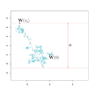
(a) First step.

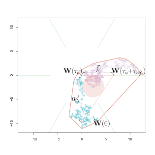
(b) Second step.

Figure 5. In the first step we wait until one of the coordinate range processes hits value $a$. For simplicity, this stopping time is denoted by $\tau_{a}$, that is, $\tau_{a}=\min\{\Theta^{R_{1}}(a),\Theta^{R_{2}}(a)\}$. The trajectory up to this random time is colored blue. At this random time, the convex hull contains a line segment of length at least $a$ and $\mathbf{W}$ is positioned at one of its endpoints. Now we rotate and translate the trajectory so that this endpoint is at the origin and the mentioned line segment is oriented vertically. In the second step, we wait until $\mathbf{W}$ exits a radial slit plane with $6$ slits (colored green) and radius $r$. The trajectory corresponding to the second step is colored purple. In the end, one of the triangles shown in Figure 4 will be contained in the convex hull of the trajectory.

∎

5. A few words on Monte Carlo simulations

In this section we provide a few more details about the simulations we performed to obtain estimates of the expected values of all the random variables that we are studying in this paper. In addition to giving us the estimates of the true value of those expected values, the simulations also give us information on how sharp the bounds we have obtained are, and where one has the most space for improvement, cf. Table 1. To be able to extract more information from the simulations, for each simulation of the trajectory of the Brownian motion we calculated values of all the variables we were interested in – perimeter, area, diameter, circumradius and inradius of the convex hull of that trajectory run up to time $1$, and the time when the perimeter, area, diameter, circumradius and inradius of the convex hull of that trajectory attained value $1$ for the first time. In this way we have simulated realizations of the random vector that comprises of all those random variables. This enabled us to estimate some other interesting quantities such as the ones appearing in Remark 3.1 and Remark 3.2. We simulated $10^{6}$ trajectories of Brownian motion, so we had $10^{6}$ realizations of the mentioned random vector.

To perform the simulations we used Python [24]. After simulating Brownian motion and calculating the convex hull (which can be done with built-in functions), we had to calculate the functionals that we are interested in – perimeter, area, diameter, circumradius and inradius. Since the function for calculating the convex hull returns extremal points of the convex hull (in clockwise order), it is then straightforward to calculate perimeter, area and diameter. Calculating the circumradius and inradius is, however, a bit more challenging. Luckily, for the circumradius, one can apply the well-known Welzl’s algorithm; see [26]. We include a few more words on the issue of calculating the inradius in the following subsection.

5.1. Inradius and Chebyshev’s center

To obtain a Monte Carlo estimation of the expected value of the inradius of the convex hull of the trajectory of the planar Brownian motion up to time $1$, and the expected value of the time when the inradius of the convex hull of the trajectory of planar Brownian motion attains value $1$, we make use of the notion of Chebyshev’s center for sets. Below we provide a brief definition of Chebyshev’s center in a general setting, and then we explain how we used it in the present framework. For what follows we refer to [3, Section 8.5.1].

Let $C\subset\mathbb{R}^{n}$ be a bounded set with nonempty interior. A Chebyshev’s center is a center of the largest ball that lies inside $C$. Figure 1 shows an example where the set $C$ is exactly the convex hull of the trajectory of planar Brownian motion up to time $1$.

When the set $C$ is convex, computing Chebyshev’s center is a convex optimization problem. More specifically, suppose $C\subset\mathbb{R}^{n}$ is defined by a set of inequalities:

$$C=\{x\in\mathbb{R}^{n}\mid f_{1}(x)\leq 0,\ldots,f_{m}(x)\leq 0\},$$

where the functions $f_{1},\ldots,f_{m}$ are all convex. A Chebyshev’s center of $C$ is defined as a solution to the following optimization problem

maximize $$\quad\rho$$ (48)

subject to $$\quad g_{i}(x,\rho)\leq 0,\quad i=1,\ldots,m,$$

where $g_{i}$ is defined as

$$g_{i}(x,\rho)=\sup_{\norm{u}\leq 1}f_{i}(x+\rho u).$$

Since each function $g_{i}$ is the pointwise maximum of a family of convex functions, it is itself convex, and thus problem (48) is a convex optimization problem, However, evaluating $g_{i}$ involves solving a convex maximization problem (either numerically or analytically), which may be very hard. In practice, one can find Chebyshev’s center only in cases when the functions $g_{i}$ are easy to evaluate. Fortunately, for the sake of our simulations, we only need to find Chebyshev’s center for polygons in $\mathbb{R}^{2}$.

If the set $C$ is a polyhedron in $\mathbb{R}^{d}$, i.e., it is defined by a set of linear inequalities $a_{i}^{T}x\leq b_{i}$, $i=1,2,\ldots,m$ (where $a^{T}$ is the transpose of vector $a$), we have

$$g_{i}(x,\rho)=\sup_{\norm{u}\leq 1}a_{i}^{T}(x+\rho u)-b_{i}=a_{i}^{T}x+\rho\norm{a_{i}}-b_{i}.$$

Hence, Chebyshev’s center can be found by solving the following linear problem

maximize $$\quad\rho$$

subject to $$\quad a_{i}^{T}x+\rho\norm{a_{i}}\leq b_{i},\quad i=1,\ldots,m$$

$$\quad\rho\geq 0$$

with variables $x$ and $\rho$.

5.2. Numerical results

Even though we could extract more information from our simulations, we give only a brief summary of our results; see Table 1. To check the accuracy of our simulations, we also calculated the estimated values for the mean of the perimeter and the area of the convex hull of the trajectory of planar Brownian motion run up to time $1$, even though these values are known explicitly. Comparing results obtained using simulations with the true values, we could see that the error exhibited by the simulations is of the order $10^{-3}$. Moreover, according to our simulations, we estimate the mean of the diameter of the convex hull of the trajectory of planar Brownian motion run up to time $1$ to be approximately $1.99$. This corroborates the estimate obtained by simulation in [16].

5.3. Numerical evaluation of the second moment of the perimeter

As already mentioned in the introduction, the authors of [25] gave the following integral expression for the second moment of the perimeter of the convex hull of the planar Brownian motion run up to time $1$,

$$\mathbb{E}\left[\mathsf{P}^{2}\right]=4\pi\int_{-\frac{\pi}{2}}^{\frac{\pi}{2}}\int_{0}^{\infty}\cos\theta\frac{\cosh(u\theta)}{\sinh(u\pi/2)}\tanh\left(\frac{2\theta+\pi}{4}u\right)\mathop{\mathrm{d}u}\mathop{\mathrm{d}\theta}.$$

There are two problematic issues concerning the integral above, namely dividing by zero when $u=0$, and overflow in $\cosh$ and $\sinh$ when $u$ becomes big. It turns out that both of these problems can be removed with the aid of some simple symbolic manipulations. To solve the problem that appears at infinity, one can rewrite $\cosh$ and $\sinh$ using the definition, and then divide by the fastest growing term. This gives us

$$\frac{\cosh(u\theta)}{\sinh(u\pi/2)} =\frac{e^{u\theta}+e^{-u\theta}}{e^{u\pi/2}-e^{-u\pi/2}}=\frac{e^{u(\theta-\pi/2)}+e^{-u(\theta+\pi/2)}}{1-e^{-u\pi}}.$$

Furthermore, to get rid of the problem at $u=0$, we use the fact that $\tanh(x)=\frac{1-e^{-2x}}{1+e^{-2x}}$, which results in

$$\frac{\cosh(u\theta)}{\sinh(u\pi/2)}\tanh\left(\frac{2\theta+\pi}{4}u\right) =\frac{e^{u(\theta-\pi/2)}+e^{-u(\theta+\pi/2)}}{1-e^{-u\pi}}\cdot\frac{1-e^{-u\theta-u\pi/2}}{1+e^{-u\theta-u\pi/2}}$$

$$=\frac{e^{u(\theta-\pi/2)}+e^{-u(\theta+\pi/2)}}{1+e^{-u\theta-u\pi/2}}\cdot\frac{1-e^{-u\theta-u\pi/2}}{1-e^{-u\pi}}.$$

We observe that the function

$$u\mapsto\frac{1-e^{-u\theta-u\pi/2}}{1-e^{-u\pi}}$$

is no longer problematic at $u=0$ as it holds that

$$\lim_{u\to 0}\frac{1-e^{-u\theta-u\pi/2}}{1-e^{-u\pi}}=\frac{1}{2}+\frac{\theta}{\pi}.$$

After making the modifications described above, Mathematica was able to numerically evaluate the integral without issue. More specifically, we used the command NIntegrate with the following options: WorkingPrecision$\rightarrow$200, Method$\to$‘‘GaussKronrodRule’’, Exclusions$\to${$\theta$==$-\pi/2$,$\theta$==$\pi/2$}, and AccuracyGoal$\to$10. We were able to reproduce the same result in MATLAB using the command integral2, with the following options: ‘Method’, ‘iterated’, ‘AbsTol’, 1e-25, ‘RelTol’, 1e-10. As reported in (3), the estimated value of the integral is $26.209056$.

References

• [1] A. Akopyan and V. Vysotsky. Large deviations of convex hulls of planar random walks and Brownian motions. Ann. H. Lebesgue, 4:1163–1201, 2021.
• [2] P. Biane, J. Pitman, and M. Yor. Probability laws related to the Jacobi theta and Riemann zeta functions, and Brownian excursions. Bull. Amer. Math. Soc. (N.S.), 38(4):435–465, 2001.
• [3] S. Boyd and L. Vandenberghe. Convex optimization. Cambridge University Press, Cambridge, 2004.
• [4] B. M. Brown. Formulae for absolute moments. J. Austral. Math. Soc., 13:104–106, 1972.
• [5] D. L. Burkholder. Exit times of Brownian motion, harmonic majorization, and Hardy spaces. Advances in Math., 26(2):182–205, 1977.
• [6] M. Cranston, P. Hsu, and P. March. Smoothness of the convex hull of planar Brownian motion. Ann. Probab., 17(1):144–150, 1989.
• [7] M. El Bachir. L’enveloppe convexe du mouvement brownien, 1983.
• [8] W. Feller. The asymptotic distribution of the range of sums of independent random variables. Ann. Math. Statistics, 22:427–432, 1951.
• [9] R. Garbit and K. Raschel. An improved lower bound for the expected diameter of planar brownian motion. unpublished manuscript.
• [10] I. S. Gradshteyn and I. M. Ryzhik. Table of integrals, series, and products. Elsevier/Academic Press, Amsterdam, eighth edition, 2015. Translated from the Russian, Translation edited and with a preface by Daniel Zwillinger and Victor Moll, Revised from the seventh edition [MR2360010].
• [11] J.-P. Imhof. On the range of Brownian motion and its inverse process. Ann. Probab., 13(3):1011–1017, 1985.
• [12] M. Jovalekić. Lower bound for the diameter of planar Brownian motion. Bull. Math. Soc. Sci. Math. Roumanie (N.S.), 64(112)(3):281–284, 2021.
• [13] G. Letac and L. Takacs. Problems and Solutions: Solutions of Advanced Problems: 6230. Amer. Math. Monthly, 87(2):142, 1980.
• [14] P. Lévy. Processus Stochastiques et Mouvement Brownien. Suivi d’une note de M. Loève. Gauthier-Villars, Paris, 1948.
• [15] S. N. Majumdar, A. Comtet, and J. Randon-Furling. Random convex hulls and extreme value statistics. J. Stat. Phys., 138(6):955–1009, 2010.
• [16] J. McRedmond and C. Xu. On the expected diameter of planar Brownian motion. Statist. Probab. Lett., 130:1–4, 2017.
• [17] P. Mörters and Y. Peres. Brownian motion, volume 30 of Cambridge Series in Statistical and Probabilistic Mathematics. Cambridge University Press, Cambridge, 2010. With an appendix by Oded Schramm and Wendelin Werner.
• [18] R. Osserman. Bonnesen-style isoperimetric inequalities. Amer. Math. Monthly, 86(1):1–29, 1979.
• [19] D. Revuz and M. Yor. Continuous martingales and Brownian motion, volume 293 of Grundlehren der Mathematischen Wissenschaften [Fundamental Principles of Mathematical Sciences]. Springer-Verlag, Berlin, third edition, 1999.
• [20] L. C. G. Rogers and L. Shepp. The correlation of the maxima of correlated Brownian motions. J. Appl. Probab., 43(3):880–883, 2006.
• [21] M. A. Snipes and L. A. Ward. Harmonic measure distributions of planar domains: a survey. J. Anal., 24(2):293–330, 2016.
• [22] E. Tsukerman and E. Veomett. Brunn-Minkowski theory and Cauchy’s surface area formula. Amer. Math. Monthly, 124(10):922–929, 2017.
• [23] S. Vakeroudis and M. Yor. Integrability properties and limit theorems for the exit time from a cone of planar Brownian motion. Bernoulli, 19(5A):2000–2009, 2013.
• [24] G. Van Rossum and F. L. Drake. Python 3 Reference Manual. CreateSpace, Scotts Valley, CA, 2009.
• [25] A. R. Wade and C. Xu. Convex hulls of random walks and their scaling limits. Stochastic Process. Appl., 125(11):4300–4320, 2015.
• [26] E. Welzl. Smallest enclosing disks (balls and ellipsoids). In New Results and New Trends in Computer Science: Graz, Austria, June 20–21, 1991 Proceedings, pages 359–370. Springer, 2005.
• [27] D. V. Widder. The Laplace Transform. Princeton University Press, Princeton, N. J.,,, 1941.