Batched Predictors Generalize within Distribution

Abstract

We study the generalization properties of batched predictors, i.e., models tasked with predicting the mean label of a small set (or batch) of examples. The batched prediction paradigm is particularly relevant for models deployed to determine the quality of a group of compounds in preparation for offline testing. By utilizing a suitable generalization of the Rademacher complexity, we prove that batched predictors come with exponentially stronger generalization guarantees as compared to the standard per-sample approach. Surprisingly, the proposed bound holds independently of overparametrization. Our theoretical insights are validated experimentally for various tasks, architectures, and applications.

1 Introduction

Generalization is arguably the most desirable property of any supervised machine learning algorithm. We currently possess an extensive theory about how well a predictive model performs in an unseen example from the training distribution. Standard results in learning theory assert that generalization is possible if one makes assumptions about the size of the hypothesis class and distribution, but the No-Free-Lunch theorem reveals that universal guarantees are generally unattainable  [1, 2].

We diverge from the usual supervised learning perspective and introduce the problem of batched prediction: rather than asking for per-sample guarantees, the model is now tasked with predicting the mean label of a batch of $k$ samples, with $k$ being a small integer (see Figure 1).

Our study is relevant to scenarios where one relies on predictive models to assess the average quality of a set of examples, typically in preparation for more expensive and offline testing [3]. Such problems arise, for example, when testing compounds for biochemical activity. Therein, one typically aims to identify a group of compounds with desirable properties, such as low toxicity and target-specific activity. Before submitting a batch of designs for experimental validation, it is common to use predictive models to assess the probability that some portion of the proposed designs has the desired property [4, 5, 6, 7, 8, 9].

From a theoretical standpoint, we aim to determine how generalization in batched learning differs from the standard case when $k$ is a small integer greater than 1. Intuitively, this should be a simpler task than standard supervised learning ($k=1$) since the model is penalized less for providing a high variance estimate of the true label. Indeed, when $k\to\infty$ batched prediction simplifies to estimating the mean label; a problem that is easily solvable. It is also intriguing to consider whether there is a significant difference in how fast measure concentrates in this setting since the number of batched samples increases exponentially with $k$ for a fixed size training set $n$. We ask, does sample complexity improve if we build exponentially many batches from the same number of $n$ examples considering that the information that we have about the true labels has not changed?

The main contribution of this manuscript entails providing a positive answer to the above question. By extending the Rademacher complexity argument to the batched prediction problem, we show that increasing $k$, even slightly, can lead to significant generalization gains. Surprisingly, we discover that the gains obtained exhibit an exponential dependency on the batch size $k$. As is common in Rademacher-type arguments, our generalization bound has two terms corresponding to (a) the difference in generalization between a typical and a sampled training set; and (b) the generalization error averaged over random draws of the $n$ training samples. Our analysis determines a divide between the above two terms: whereas the former remains unchanged, the latter is exponentially smaller as a function of $k$. The exponential gains are particularly attractive since the average-case generalization error term is the only one that exhibits any dependency on the class of models harnessed for prediction. The above findings have a striking consequence: for batches as small as $k=2$, it is possible to obtain universal generalization bounds, i.e., bounds that hold irrespective of how much the classifier is overparametrized .

As a further contribution, we show that batched predictors can be trained in exactly the same manner as standard per-sample predictors and thus any per-sample predictor can be turned into a batched predictor without additional training requirements. To this end, we analyze the relationship between the risks of varying prediction batch-size $k$. We show that, under mild assumptions, the $1$-risk provides an upper bound on any $k$-risk for $k>1$. This implies that standard 1-risk minimization can be used as a training objective even when a batched prediction task is considered.

We stress that the notion of prediction batch is unrelated to the concept of mini-batch of stochastic gradient descent (SGD) training. In batched prediction, the prediction task of the model is changed, i.e., the model aims to estimate the mean label on the prediction batch. In contrast, mini-batched SGD training does not change the prediction task. The mini-batch is merely used to obtain a Monte Carlo estimator for the gradient of the training objective.

Our theoretical results are verified across different architectures (graph neural networks, convolutional neural networks), application domains (antibody design, quantum chemistry), and tasks (regression and classification). The numerical results corroborate our theory, showing that the $k$-risk generalization error is indeed reduced significantly with increasing prediction batch size $k$. The practical implication of our findings are twofold: (a) the current paradigm of learning suffices also for batched prediction; (b) since batched predictors that fit the training data are shown to have good generalization guarantees, the violation of the within-distribution assumption is a likely culprit behind possible poor batched generalization.

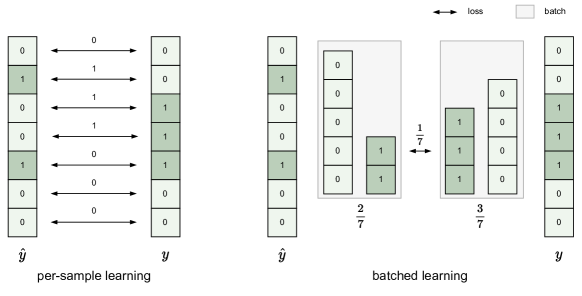
Figure 1: Illustration of batched learning for binary classification. Left-hand side shows the standard learning setting: predictions $\hat{y}$ for samples are compared to ground truth labels $y$ individually across the batch. Right-hand side shows the case of batched learning: only the total number of positives (and consequently the number of negatives) in a given prediction batch is compared.

1.1 Related work

In the following, we provide references and discuss connections with previous analyses, applications, and machine learning paradigms.

Study of generalization.

There is an extensive body of work studying the generalization of standard classifiers, e.g., based on VC-dimension [10], Rademacher complexity [11], PAC-Bayes [12, 13, 14, 15, 16, 17, 18, 19] robustness [20, 21, 22], Neural Tangent Kernel [23], and stability arguments [24, 25, 26, 27, 28]. For a pedagogical review of learning theory, we refer the reader to [2], whereas a modern critical analysis of generalization for deep learning can be found in  [29]. To the extent of our knowledge, the batched prediction problem this manuscript focuses on has not been previously considered.

Batched screening of molecular libraries.

The tailored design of forecasting models for batched biological sequence classification was previously considered by [3]. Therein, the label posterior of experimental libraries is approximated by a Gaussian mixture model. The practical approach attempts to also account for distribution shift and is numerically shown to improve upon models trained to do standard classification. Our work provides a complementary perspective by elucidating the fundamental generalization limits of batched predictors.

Model calibration.

A calibrated classifier has the property that it produces probabilistic predictions that match the true fraction of positives and thus quantify the uncertainty of a model’s prediction [30, 31, 32]. In the case of $k=n$, batched learning boils down to a mild form of model calibration, where only the mean behavior of the classifier is considered. The two problems are distinct when $k$ is a small constant.

Conformal prediction.

A loose parallel can be drawn between conformal and batched prediction: whereas the former provides generalization guarantees by considering classifiers that output sets of possible labels, we here study the generalization when predicting the average label of a set of inputs. We refer to [33] for a recent review.

2 The batched prediction problem

This section defines the batched learning task formally and compares it to the standard case of per-sample prediction.

Per-sample prediction.

In a standard supervised learning task, we assume that the data $z=(x,y)\in\mathbb{Z}=\mathbb{X}\times\mathbb{Y}$ is independent and identically distributed (i.i.d.) with respect to the data distribution $\mathcal{D}$ supported over the domain $\mathbb{Z}$. One then aims to learn a model $f:\mathbb{X}\to\mathbb{Y}$ which minimizes the expected risk

$$r(f,\mathcal{D})=\mathbb{E}_{z\sim\mathcal{D}}\left[l(f(x),y)\right]\,,$$ (1)

where $l:\mathbb{Z}\to\mathbb{R}$ is an appropriately chosen loss function for the task at hand and may, for example, take the form

$$l(x,y)=(x-y)^{2}\,, l(x,y)=\frac{1}{2}(1-x\,y)\,, l(x,y)=-y\log x$$ (2)

for the mean-squared error, zero-one, and cross-entropy loss, respectively. The expected risk is usually intractable as it involves an expectation value over the data distribution. One therefore minimizes the empirical risk over a training set $Z=\left\{(x_{i},y_{i})\right\}^{n}_{i=1}$ instead:

$$r(f,Z)=\hat{E}_{Z}\left[l(f(x),y)\right]\,,$$ (3)

where we used the following notation for the sample mean

$$\hat{E}_{Z}\left[g(z)\right]=\frac{1}{|Z|}\sum_{z\in Z}g(z)$$ (4)

for any function $g$. Note that the empirical risk is an unbiased estimator of the expected risk.

Batched prediction.

A supervised learning task for a batched predictor takes a closely related but different form. Concretely, we consider batches of data $S=\left\{(x_{i},y_{i})\right\}^{k}_{i=1}$ of $k$ samples drawn i.i.d. from the data distribution $\mathcal{D}$ and aim to predict the average label over the batch $\hat{E}_{S}\left[y\right]$ by the average prediction $\hat{E}_{S}\left[f(x)\right]$. That is, we aim to train the model $f$ such that

$$\hat{E}_{S}\left[f(x)\right]=\hat{E}_{S}\left[y\right]\,.$$ (5)

This corresponds to correctly predicting the fraction of binders within a batch in the example of molecular design.

To this end, it is natural to define the expected $k$-risk

$$r_{k}(f,\mathcal{D})=\mathbb{E}_{S\sim\mathcal{D}^{k}}\left[l(\hat{E}_{S}\left[f(x)\right],\hat{E}_{S}\left[y\right])\right]\,,$$ (6)

where $\mathcal{D}^{k}$ denotes the distribution over all $k$-sets drawn i.i.d. from the data distribution $\mathcal{D}$. Due to the expectation value over this distribution, the expected risk is again intractable. One therefore defines the empirical $k$-risk

$$r_{k}(f,Z)=\hat{E}_{S\subset_{k}Z}\left[l(\hat{E}_{S}\left[f(x)\right],\hat{E}_{S}\left[y\right])\right]$$ (7)

which is an unbiased estimator of the expected $k$-risk, see Supplementary Material for proof. Here, we have introduced the notation

$$\hat{E}_{S\subset_{k}Z}\left[g(S)\right]=\frac{1}{\binom{n}{k}}\sum_{S\subset_{k}Z}g(S)\,,$$ (8)

where the sum runs over all subsets of cardinality $k$ of the training set $Z$.

3 Properties of $k$-risk and the training of batched predictors

In the following, we derive a number of useful properties of $k$-risk. These illuminate the effect of the batch size $k$ and argue that a convenient way to minimize $k$-risk is by minimizing $1$-risk as usual.

An obvious property of the $k$-risk is that it reduces to the standard risk (3) used for per-sample prediction in the case of $k=1$. In the opposite limit $k\to\infty$, it takes a particular simple form:

$$\lim_{k\to\infty}r_{k}(f,\mathcal{D})=l(\mathbb{E}_{\mathcal{D}}[f(x)],\mathbb{E}_{\mathcal{D}}[y])\,,$$ (9)

which is minimized by the constant function $f(x)=\mathbb{E}_{\mathcal{D}}[y]$. This function can straightforwardly be learned to high accuracy by the mean predictor $\hat{E}_{Z}[y]$ over the training set $Z$ as can be easily shown using a standard concentration of measure argument. Similarly, the empirical risk $r_{n}(f,Z)$ is minimized by the mean predictor over the training set $Z=\left\{z_{i}\right\}^{n}_{i=1}$ and $k=n$ is the maximal value $k$ can take during training since there are only $n$ samples in the training set.

Our first result entails showing that for many loss functions of practical interest, any empirical $k$-risk can be written as a convex sum of $r_{n}(f,Z)$, corresponding to the maximal $k$ value during training, and empirical risk $r_{1}(f,Z)$, corresponding to the minimal value for $k$:

Property 1.

The empirical $k$-risk $r_{k}(f,Z)$ can be written as convex combination of the empirical $1$-risk and $n$-risk

$$r_{k}(f,Z)=(1-a_{k,n})\,r_{1}(f,Z)+a_{k,n}\,r_{n}(f,Z)$$ (10)

for the mean-squared error, zero-one, and geometric mean cross entropy loss with

$$a_{k,n}=\frac{n(k-1)}{k(n-1)}\in[0,1]\,.$$ (11)

This relation enables efficient calculation of all $k$-risks as we do not need to average over the corresponding subsets of size $k$; a convenient property given that the number of the subsets grows exponentially with $k$.

So how should one minimize $k$-risk during training? As minimizing the empirical risk over the entire training set $r_{n}(f,Z)$ can be minimized by the constant mean predictor, it is reasonable to posit that one can also minimize the $k$-risk by minimizing the $1$-risk. The following theorem shows that, under mild assumptions on the loss function, this is indeed the case:

Property 2.

Let $l(x,y)$ be a doubly-convex loss function. Then, it holds that

$$r_{k}(f,\mathcal{D})\geq r_{k^{\prime}}(f,\mathcal{D})$$ (12)

for any $k\leq k^{\prime}$.

Property 2 is handy as it implies that we do not need to change the training process: standard $1$-risk minimization suffices to also minimize $k$-risk. In other words, we can simply minimize the $1$-risk during training and thereby simultaneously minimize all $k$-risks for $k>1$, since the $1$-risk provides an upper bound for them. This result may be intuitively understood by the fact that it is considerably harder for the model to accurately predict each sample in the batch individually. If the model is sufficiently powerful to do so, it can also perfectly predict the frequency over the batch, i.e., it can perfectly perform batched prediction as well.

It is worth stressing that the theorem applies to a broad class of optimization criteria since any loss derived from an $f$-divergence, in particular from a KL-divergence, is doubly convex. In more detail, any loss of the form $l(\hat{y},y)=\hat{y}\,g(y/\hat{y})$ with convex $g$, is doubly convex. For the Kullback-Leibler divergence, this function takes the form $g(x)=x\log(x)$.

An interesting subtlety arises in the case of classification which is often trained using a binary cross-entropy loss:

$$\textrm{bce}(\hat{y},y)=-y\log(\hat{y})-(1-y)\log(1-\hat{y})\,.$$ (13)

This training objective is widely used since it agrees with the Kullback-Leibler divergence $\textrm{kl}(y,\hat{y})$ up to a model-independent term that only depends on the labels $y$. As a result, the binary cross entropy and KL divergence have identical gradients with respect to the model’s parameters. The latter implies that the binary-cross entropy can be optimized as a proxy for the KL divergence. However, the binary cross entropy is not a doubly-convex loss function, as it is only convex with respect to its last but not with respect to both arguments [34]. The lack of double convexity, however, is of no concern since we are really interested in minimizing the Kullback-Leibler divergence. For classification, we can thus train a batched predictor in exactly the same way as a standard per-sample predictor, i.e., by optimizing the cross entropy loss for $k=1$ and thereby minimizing the Kullback-Leibler divergence for all $k\geq 1$. We refer to the Supplement for a more detailed discussion of this point. The mean-squared error loss is doubly convex and thus no such subtleties arise in the case of regression.

4 Generalization of batched predictors

While batched predictors can be trained by minimizing the same risk as in the standard setting, this section shows that they come with considerably different generalization guarantees.

We analyze the following regression and classification setups:

1. Classification with a zero-one loss and $\mathbb{Y}=\{-1,1\}$.

2. Regression with a mean-squared error loss and $\mathbb{Y}=[0,1]$.

For the above, we bound the generalization error in terms of a suitable generalization of the Rademacher complexity:

Definition 1 ($k$-Rademacher complexity).

The empirical $k$-Rademacher complexity is

$$\hat{\mathcal{R}}_{k,n}(l\circ\mathcal{F})=\mathbb{E}_{(\sigma_{S})_{S\subset_{k}Z}}\left[\sup_{f\in\mathcal{F}}\hat{E}_{S\subset_{k}Z}\left[\sigma_{S}\,l(\hat{E}_{S}\left[f(x)\right],\hat{E}_{S}\left[y\right])\,\right]\right],$$ (14)

where $\sigma_{S}$ denotes Rademacher random variables and $\mathcal{F}$ is the hypothesis class from which the model is chosen. The expected $k$-Rademacher complexity is

$$\mathcal{R}_{k,n}(l\circ\mathcal{F})=\mathbb{E}_{Z\sim\mathcal{D}^{n}}\left[\hat{\mathcal{R}}_{k,n}(l\circ\mathcal{F})\right]\,.$$ (15)

The above reduces to the standard Rademacher complexity for the case of $k=1$.

With these definitions in place, the following result is derived in the Supplementary Material:

Theorem 1 (Generalization bound).

Let $l:\mathbb{X}\times\mathbb{Y}\to\mathbb{R}$ be a Lipschitz continuous loss with Lipschitz constant $\lambda$ and $\mathbb{Y}\subset[a,b]$. Then, it holds for all $f\in\mathcal{F}$ that

$$r_{k}(f,\mathcal{D})\leq r_{k}(f,Z)+2\,\mathcal{R}_{k,n}(l\circ\mathcal{F})+c\,\sqrt{\frac{\ln\tfrac{1}{\delta}}{n}}$$ (16)

with probability at least $1-\delta$ and $c=\lambda|a-b|$.

For classification, this result can then be used to derive the following corollary which bounds the generalization error in terms of the shattering coefficient:

$$S_{\mathcal{F}}(n)=\max_{Z\subset_{n}\mathbb{Z}}\left|\mathcal{F}_{Z}\right|\quad\text{with}\quad\mathcal{F}_{Z}=\{f(x_{1}),\dots,f(x_{n})|\,f\in\mathcal{F}\}.$$

Specifically, we show in the Supplement that:

Corollary 1 (Universal generalization).

Consider classification with the above assumptions. Then, it holds for all $f\in\mathcal{F}$ with shattering coefficient $S_{\mathcal{F}}(n)$ that

$$r_{k}(f,\mathcal{D})-r_{k}(f,Z)\leq\underbrace{\sqrt{\frac{2\ln S_{\mathcal{F}}(n)}{\binom{n}{k}}}}_{\xi(|\mathcal{F}|;n,k)}+\underbrace{\sqrt{\frac{\ln\tfrac{1}{\delta}}{n}}}_{\psi(n,\delta)}=O\left(n^{\tfrac{-(k-1)}{2}}+\sqrt{\frac{\ln\tfrac{1}{\delta}}{n}}\right)$$ (17)

with probability at least $1-\delta$ and $k=O(1)$.

This result is to be compared with the standard one for the per-sample predictor which is recovered for $k=1$. We compare the two terms for both the standard and batched case separately:

(a) Expected generalization error ($\mathcal{F}$ dependent term). Term $\xi(|\mathcal{F}|;n,k)$ is exponentially smaller than the standard one $\xi(|\mathcal{F}|;n,1)$:

$$\frac{\xi(|\mathcal{F}|;n,k)}{\xi(|\mathcal{F}|;n,1)}=\sqrt{\frac{n}{\binom{n}{k}}}\leq\frac{k^{\frac{k}{2}}}{n^{(k-1)/2}}=O(n^{-(k-1)})$$ (18)

This property is striking as in the standard term the numerator of $\xi(|\mathcal{F}|;n,1)$ scales unfavorably compared to the denominator resulting in a loose bound unless strong assumptions are made about the hypothesis class.

It is well known that, for binary classification, a universal upper bound for the shattering coefficient is $S_{\mathcal{F}}(n)\leq 2^{n}$, which holds for any classifier by noticing that the number of possible hypotheses corresponds to all the possible ways of labeling the training set (corresponding to unbounded VC dimension). The former bound is typically not useful as

$$\xi(2^{n};n,1)=\sqrt{\frac{2n\ln 2}{n}}\geq 1,$$

which is vacuous. In contrast, the batched case term

$$\xi(2^{n};n,k)=\sqrt{\frac{2n\ln 2}{\binom{n}{k}}}\leq\sqrt{\frac{(\ln 4)k^{k}}{{n}^{k-1}}},$$

is strictly below 1 even for $k=2$ when $n>8\ln 2$. Intriguingly, the above argument asserts that even heavily overparametrized models can avoid overfitting when optimizing $k$-risk, a statement that cannot be shown in the standard setup without additional distributional, invariance, or hypothesis class assumptions [1, 2].

At an intuitive level, this exponential difference between batched and per-sample predictors may be attributed to the fact that a batched predictor is trained using $\binom{n}{k}$ samples, i.e., the subsets of size $k$ of a training set with $n$ elements. In this sense, the classifier is trained on exponentially more data.

(b) Deviation from expectation ($\mathcal{F}$ independent term). The term $\psi(n,\delta)$ does not depend on $k$ and thus agrees with the standard per-sample learning result. The exponential increase in data, in the sense discussed above, therefore does not translate into a gain in this term.

We note that Theorem 1 also holds in the case of regression with a factor of $2$ multiplying the $\delta$-dependent term and $\xi(|\mathcal{F}|;n,k)\to 4\xi(|\mathcal{F}|;n,k)$. The resulting scaling differences to the standard case are however of less relevance as the size of the hypothesis class diverges in this case and thus a more elaborate analysis is likely needed to obtain a universal bound. The case of batched regression thus constitutes a promising line of future research.

Lastly, we stress that one can easily rewrite $\xi(|\mathcal{F}|,n,k)$ in terms of the VC dimension by using Sauer’s Lemma. This rewriting does not affect the discussion of the exponential difference in scaling. We refer to the Supplement for a more detailed discussion on this point.

5 Experimental validation

We analyze the generalization properties of batched predictors experimentally in the following and demonstrate that they indeed show favorable generalization behavior as suggested by our theoretical analysis in the last section. We consider both classification and regression as well as different architectures and application domains.

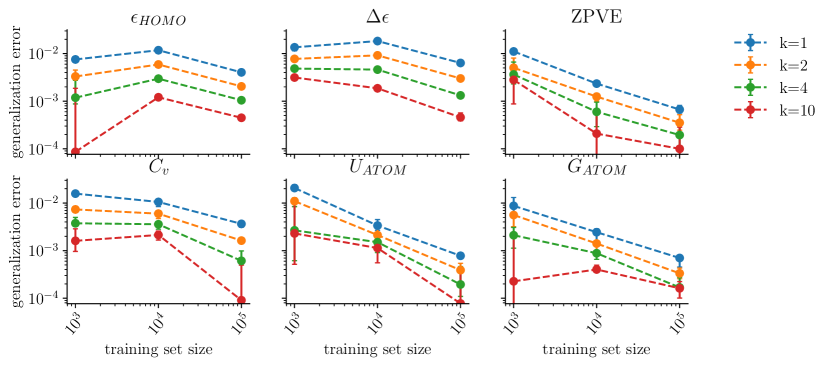
Figure 2: Estimated relative generalization error on the QM9 dataset for different training set sizes decreases with the prediction batch sizes $k$ across a wide variety of targets. We show the median of the relative mean absolute error risk, as well as the 25th and 75th percentile over three training runs for each target, initialized with different seeds. The shown targets are the highest occupied molecular orbital energy $\epsilon_{\textrm{HOMO}}$, the gap between highest and lowest occupied orbital energy $\Delta\epsilon$, zero point vibrational energy ZPVE, heat capacity $C_{v}$, atomization energy $U_{\textrm{ATOM}}$, and atomization enthalpy $G_{\textrm{ATOM}}$. The latter two quantities are with respect to a temperature of 298.15K and the estimate for the last four targets is scaled by a factor of 10 for better visual comparison.

In our experiments, we approximate the $k$-generalization error by the difference of the empirical risk on the test and training set, i.e., the $k$-generalization error:

$$\left|r_{k}(f,\mathcal{D})-r_{k}(f,Z)\right|\;\;\;\textrm{is estimated by}\;\;\;\left|r_{k}(f,T)-r_{k}(f,Z)\right|\,,$$ (19)

where $T$ denotes the test set. This estimation is repeated for several different seeds for error estimation.

5.1 Quantum chemistry: regression for molecular property prediction

We train a graph neural network to predict quantum chemical properties of small molecules. We use the QM9 dataset [35] which is one of the standard benchmarks in Quantum Chemistry and consists of 130k molecules along with regression targets, such as the heat capacity and orbital energy of the atomistic system. We use three different training sizes, namely 1k, 10k, and 100k, and estimate the generalization error using a test-set size of 10k. Hyperparameters were tuned on a validation set of the same size. In order to use a standard graph neural network, we use the same architecture as in the official PyTorch Geometric [36] example for QM9. For a more detailed discussion of the experimental setup, we refer to the Supplementary Material. Figure 2 shows the estimated generalization error for the three training set sizes. The generalization error decreases with increasing prediction batch size $k$ as is suggested by the theoretical analysis of the previous section.

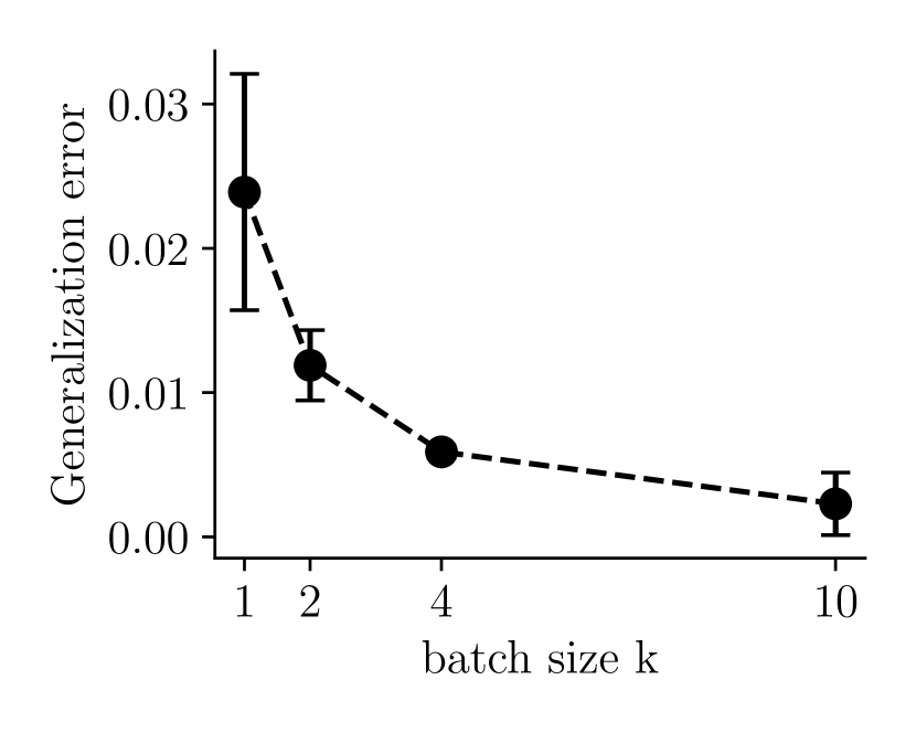
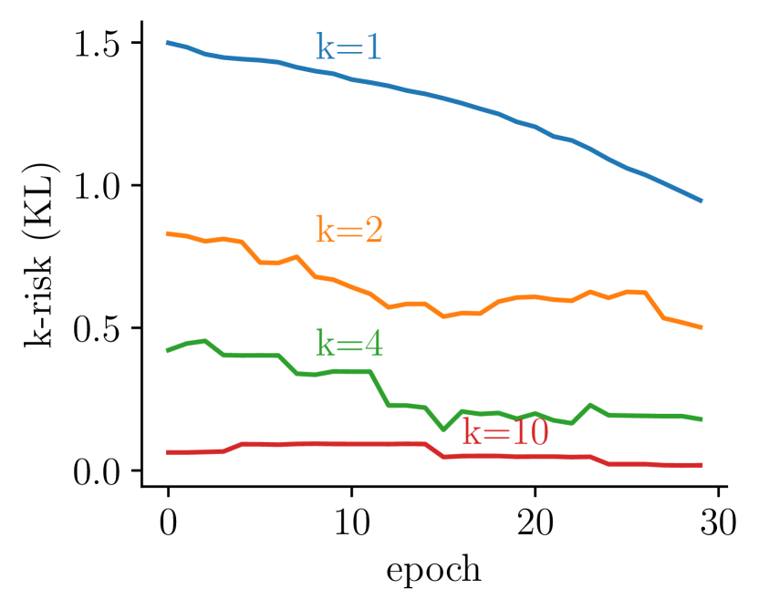
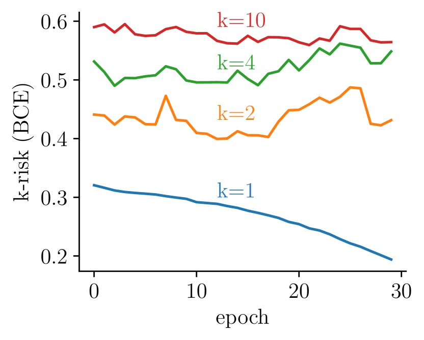
Figure 3: Left: Estimation of the generalization error of the zero-one risk on the Mason dataset for various prediction batch sizes $k$. We show the mean and standard deviation with respect to three training runs with three different initialization. Middle: Kullback-Leibler divergence decreases with prediction batch-size $k$. Right: Binary cross-entropy does not decrease with prediction batch-size $k$, as expected.

5.2 Protein design: classification of protein activity

We use the Trastuzumab CDR H3 mutant dataset [37, 38] that was constructed by mutating ten positions in the CDR H3 area of the protein Trastuzumab. The mutants were evaluated in a laboratory to determine if they bind to the HER2 breast cancer antigen. The dataset consists of sequences for 9k binders and 25k non-binders of which we use the CDR H3 region of the sequence as input to our model. We train a convolutional network to predict if the corresponding antibody binds to the HER2 antigen using a training set of 20k sequences. The generalization error is estimated using a test set of 10k sequences. We use early stopping and binary cross-entropy loss for training. More details on the architecture and training hyperparameters can be found in the Supplementary Material. The left-hand side of Figure 3 shows the estimated generalization error for the zero-one risk. Again, it can be observed that the generalization error decreases as the prediction batch size $k$ increases.

The middle of Figure 3 shows the risk based on the KL divergence for batched predictors of different prediction batch size $k$ while the corresponding cross entropy risk is shown on the right. The KL-divergence-based risk decreases as $k$ is increased, i.e., the risk for $k=1$ is an upper bound on all other risks. As expected from our discussion in Section 3, this is however not the case for the cross-entropy.

6 Limitations

Our analysis is particularly relevant to situations in which predictive models are used to select candidates for costly experimental labeling or analysis, such as in the batched biochemical testing of compounds. An important limitation of our work is that we do not consider the issue of distribution shift that often arises in the practical applications of these methods. Specifically, the change in data distribution will heavily depend on the candidates chosen by the model for experimental evaluation. This in turn will affect the generalization properties of the predictive model itself (with respect to the shifted data distribution). Analyzing the implications of this distribution shift along with a more detailed analysis of the case of regression presents a promising direction for future research.

7 Conclusion

The surprisingly strong generalization bounds for batched predictors are encouraging in light of their relevance for selecting candidates for experimental testing in applications of machine learning to chemistry and biology. Both the theoretical and numerical results obtained in this work indicate that these batched predictors may be more reliable than one might naively assume, that is, under the i.i.d. assumption. A further important insight derived in this work is that batched predictors can be trained in the same manner as standard per-sample predictors and that any per-sample predictor can be used for batched prediction without any additional training costs.

Appendix A Appendix

A.1 Empirical $k$-risk is an unbiased estimator of $k$-risk

This statement is an immediate consequence of the linearity of expectation:

$$\mathbb{E}_{Z}\left[r_{k}(f;Z)\right] =\frac{1}{n^{k}}\sum_{S=(z_{1},\ldots,z_{k})\subset Z}\mathbb{E}_{S=(z_{1},\ldots,z_{k})\sim\mathcal{D}^{k}}\left[\ell\left(\sum_{(x,y)\in S}\frac{f(x)}{k},\sum_{(x,y)\in S}\frac{y}{k}\right)\right]=r_{k}(f;\mathcal{D})$$

A.2 Proof of Property 1

Property.

The empirical $k$-risk $R_{k}(f,Z)$ can be written as convex combination of the empirical $1$-risk and $n$-risk

$$R_{k}(f,Z)=(1-a_{k,n})R_{1}(f,Z)+a_{k,n}\,R_{n}(f,Z)$$ (20)

for the mean-squared error, zero-one, and geometric mean cross entropy loss with

$$a_{k,n}=\frac{n(k-1)}{k(n-1)}\in[0,1]\,.$$ (21)

Proof.

We consider loss functions of the form:

$$l(p)=K_{1}(p)K_{2}(p)+b\,,$$ (22)

where we assume that $K_{1,2}$ are affine linear in $p$ and that $b\in\mathbb{R}$ is a constant shift. All loss functions mentioned in the theorem are of this form. Indeed, the mean-squared error loss can be obtained by

$$b =0\,,$$ (23)

$$p(z) =(f(x),y)\,,$$ (24)

$$K_{1}(p) =K_{2}(p)=f(x)-y\,.$$ (25)

While the zero-one loss can be recovered by

$$b =\frac{1}{2}\,,$$ (26)

$$p(z) =(f(x),y)\,,$$ (27)

$$K_{1}(p) =y\,,$$ (28)

$$K_{2}(p) =-\frac{1}{2}f(x)\,.$$ (29)

Finally, for the geometric-mean cross-entropy loss, we have

$$b =0\,,$$ (30)

$$p(z) =(\log f(x),y)\,,$$ (31)

$$K_{1}(p) =y\,,$$ (32)

$$K_{2}(p) =-\log f(x)\,.$$ (33)

Since $K_{1,2}(p)$ are affine linear with respect to $p$, it holds that

$$K_{1,2}\left(\frac{1}{k}\sum_{i}p_{i}\right)=\frac{1}{k}\sum_{i}K_{1,2}(p_{i})\,.$$ (34)

Note that affine linearity is not only a sufficient but also a necessary condition to fulfill this tight convexity condition.

We first consider the case of a loss function for which $b=0$ for simplicity. We can rewrite the $k$-risk as follows

$$r_{k}(f,Z) =\hat{E}_{S}\left[K_{1}\left(\frac{1}{k}\sum_{z\in S}p(z)\right)\,K_{2}\left(\frac{1}{k}\sum_{z^{\prime}\in S}p(z^{\prime})\right)\right]$$ (35)

$$=\hat{E}_{S}\left[\frac{1}{k}\sum_{z\in S}K_{1}(p(z))\,\frac{1}{k}\sum_{z^{\prime}\in S}K_{2}(p(z^{\prime}))\right]$$ (36)

$$=\hat{E}_{S}\left[\frac{1}{k^{2}}\sum_{z\in S}K_{1}(p(z))\,K_{2}(p(z))\right]+\hat{E}_{S}\left[\frac{1}{k^{2}}\sum_{z\neq z^{\prime}\in S}K_{1}(p(z))\,K_{2}(p(z^{\prime}))\right]$$ (37)

$$=\frac{1}{k}\hat{E}_{z}\left[K_{1}(p(z))\,K_{2}(p(z))\right]+\frac{k^{2}-k}{k^{2}}\hat{E}_{z\neq z^{\prime}}\left[K_{1}(p(z))\,K_{2}(p(z^{\prime}))\right]\,,$$ (38)

where we have used $\hat{E}_{S=(z_{1},\dots,z_{k})}=\hat{E}_{z_{1}}\dots\hat{E}_{z_{k}}$ in the last step. The last expression above can be rewritten as

$$\frac{1}{k}r_{1}(f,Z)+\frac{n^{2}(1-\tfrac{1}{k})}{n(n-1)}\hat{E}_{z,z^{\prime}}\left[K_{1}(p(z))\,K_{2}(p(z^{\prime}))\right]-\frac{n(1-\tfrac{1}{k})}{n(n-1)}\hat{E}_{z}\left[K_{1}(p(z))K_{2}(p(z))\right]$$

$$=\left(\frac{1}{k}-\frac{1-\tfrac{1}{k}}{n-1}\right)r_{1}(f,Z)+\frac{n(k-1)}{k(n-1)}\,\frac{1}{n}\sum_{z}\,\frac{1}{n}\sum_{z^{\prime}}K_{1}(z)K_{2}(z^{\prime})\,.$$

We now use that affine linearity of $K_{1,2}$ implies the tight convexity condition (34). Using this relation, we obtain

$$r_{k}(f,Z) =\left(\frac{1}{k}-\frac{1-\tfrac{1}{k}}{n-1}\right)r_{1}(f,Z)+\frac{n(k-1)}{k(n-1)}r_{n}(f,Z)$$ (39)

$$=(1-a_{k,n})r_{1}(f,Z)+a_{k,n}\,r_{n}(f,Z)\,,$$ (40)

where we have defined $a_{k,n}=\frac{n(k-1)}{k(n-1)}$.

The above proof for $b=0$ implies immediately for $b\neq 0$ that

$$r_{k}(f,Z)-b =(1-a_{k,n})(r_{1}(f,Z)-b)+a_{k,n}\,(r_{n}(f,Z)-b)\,,$$ (41)

and since $(1-a_{k,n})b+a_{k,n}b=b$, it follows that

$$r_{k}(f,Z) =(1-a_{k,n})R_{1}(f,Z)+a_{k,n}\,r_{n}(f,Z)\,,$$ (42)

for the general case of $b\neq 0$. ∎

A.3 Proof of Property 2

Property.

Let $l(x,y)$ be a doubly-convex loss function. Then, it holds that

$$r_{k}(f,\mathcal{D})\geq r_{k^{\prime}}(f,\mathcal{D})$$ (43)

for any $k\leq k^{\prime}$.

Proof.

Note that we can rewrite an average over a set with $k$ elements as an average over all possible sets of $k-1$ elements contained in the set of size $k$:

$$\frac{1}{k}\sum_{i=1}^{k}f(x_{i})=\frac{1}{k}\sum_{i=1}^{k}\frac{1}{k-1}\sum_{j=1\atop i\neq j}^{k}f(x_{j})\,.$$ (44)

The expected $k$-risk can be thus written as

$$r_{k}(f,\mathcal{D}) =\mathbb{E}_{z_{1},\dots,z_{k}}\left[l\left(\frac{1}{k}\sum_{i=1}^{k}f(x_{i}),\,\frac{1}{k}\sum_{i=1}^{k}y_{i}\right)\right]$$ (45)

$$=\mathbb{E}_{z_{1},\dots,z_{k}}\left[l\left(\frac{1}{k}\sum_{i=1}^{k}\frac{1}{k-1}\sum_{j=1\atop i\neq j}^{k}f(x_{j}),\,\frac{1}{k}\sum_{i=1}^{k}\frac{1}{k-1}\sum_{j=1\atop i\neq j}^{k}y(x_{j})\right)\right]$$ (46)

Since the loss function $l$ is doubly convex

$$l(\lambda x_{1}+(1-\lambda)x_{2},\lambda y_{1}+(1-\lambda)y_{2})\leq\lambda\,l(x_{1},y_{1})+(1-\lambda)\,l(x_{2},y_{2}),$$ (47)

for $\lambda\in[0,1]$, we can apply Jensen’s inequality to obtain

$$r_{k}(f,\mathcal{D}) \leq\frac{1}{k}\sum_{i=1}^{k}\mathbb{E}_{z_{1}}\dots\mathbb{E}_{z_{k}}\left[\,l\left(\frac{1}{k-1}\sum_{j=1\atop i\neq j}^{k}f(x_{j}),\frac{1}{k-1}\sum_{j=1\atop i\neq j}^{k}y_{j}\right)\right]$$ (48)

$$=\mathbb{E}_{z_{1}}\dots\mathbb{E}_{z_{k-1}}\left[l\left(\frac{1}{k-1}\sum^{k-1}_{j=1}f(x_{j}),\frac{1}{k-1}\sum_{j=1}^{k-1}y_{j}\right)\right]$$ (49)

$$=r_{k-1}(f,\mathcal{D})\,.$$ (50)

We thus obtain

$$r_{k}(f,\mathcal{D})\geq r_{k-1}(f,\mathcal{D})\geq\dots\geq r_{k^{\prime}}(f,\mathcal{D})\,,$$ (51)

for any $k\leq k^{\prime}$ as was stated in the theorem. ∎

Appendix B Proof of Theorem 1

We first derive the following technical lemma:

Lemma 1.

Let $l$ be a Lipschitz continuous loss function with Lipschitz constant $\lambda$ and $\mathbb{Y}=[a,b]$. Then, the maximal generalization error

$$\varphi_{k}(Z)=\sup_{f\in\mathcal{F}}\left(r_{k}(f,\mathcal{D})-r_{k}(f,Z)\right)$$ (52)

obeys the bounded difference condition

$$\left|\varphi_{k}(Z)-\varphi_{k}(Z^{\prime})\right|\leq\frac{\sqrt{2}c}{n}\,,$$ (53)

where we have used the notation

$$Z=\{z_{1},\dots,z_{j},\dots,z_{n}\} Z^{\prime}=\{z_{1},\dots,z^{\prime}_{j},\dots,z_{n}\}\,.$$ and (54)

and $c=\lambda|a-b|$.

Proof.

We first rewrite the difference as

$$\left|\varphi_{k}(Z)-\varphi_{k}(Z^{\prime})\right| =\left|\sup_{f\in\mathcal{F}}\left(r_{k}(f,\mathcal{D})-r_{k}(f,Z)\right)-\sup_{f\in\mathcal{F}}\left(r_{k}(f,\mathcal{D})-r_{k}(f,Z^{\prime})\right)\right|$$ (55)

$$\leq\sup_{f\in\mathbb{F}}\left|r_{k}(f,Z)-r_{k}(f,Z^{\prime})\right|\,,$$ (56)

where we have used that $\sup_{x}f_{1}(x)-\sup_{x}f_{2}(x)\leq\sup_{x}(f_{1}(x)-f_{2}(x))$ in the last step. The $k$-risk $r_{k}(f,Z)$ involves an average over all possible $k$-subsets of the set $Z$

$$\left|\varphi_{k}(Z)-\varphi_{k}(Z^{\prime})\right| \leq\sup_{f\in\mathcal{F}}\left|\hat{E}_{S\subset_{k}Z}\left[l(\hat{E}_{S}\left[f(x)\right],\hat{E}_{S}\left[y\right])\right]-\hat{E}_{S^{\prime}\subset_{k}Z^{\prime}}\left[l(\hat{E}_{S^{\prime}}\left[f(x^{\prime})\right],\hat{E}_{S}\left[y^{\prime}\right])\right]\right|.$$

For notational convenience, it is useful to define $p(z)=(f^{*}(x),y)$, where $f^{*}$ is the maximizing function of the expression above. We can then rewrite the loss as a function of $p$. The above expression can thus be rewritten more compactly as

$$\left|\varphi_{k}(Z)-\varphi_{k}(Z^{\prime})\right| \leq\left|\hat{E}_{S\subset_{k}Z}\left[\,l(\hat{E}_{S}\left[p(z)\right])\,\right]-\hat{E}_{S^{\prime}\subset_{k}Z^{\prime}}\left[\,l(\hat{E}_{S^{\prime}}\left[p(z^{\prime})\right])\,\right]\right|.$$

In this difference, all $k$-sets which are common between $Z$ and $Z^{\prime}$ will cancel. We can thus rewrite this expression as an average over sets involving $z_{j}$ of $Z$ and $z^{\prime}_{j}$ of $Z^{\prime}$. This can be easily done by averaging over all $k-1$-sets of $Z/\{z_{j}\}=Z^{\prime}/\{z^{\prime}_{j}\}$ as follows

$$\left|\varphi_{k}(Z)-\varphi_{k}(Z^{\prime})\right|$$

$$\leq\underbrace{\frac{\binom{n-1}{k-1}}{\binom{n}{k}}}_{=\frac{k}{n}}\left|\hat{E}_{A\subset_{k-1}Z/\{z_{j}\}}\left[l\left(\frac{1}{k}p(z_{j})+\frac{k-1}{k}\hat{E}_{A}\left[p(z)\right]\right)-l\left(\frac{1}{k}p(z^{\prime}_{j})+\frac{k-1}{k}\hat{E}_{A}\left[p(z)\right]\right)\right]\right|\,,$$

We now use that the loss function $l$ is Lipschitz continuous:

$$\left|l(x+\delta)-l(x+\delta^{\prime})\right|\leq\lambda\,\|\delta-\delta^{\prime}\|\,.$$ (57)

to obtain

$$\left|\varphi_{k}(Z)-\varphi_{k}(Z^{\prime})\right|\leq\frac{\lambda}{n}\,\lVert p(z_{j})-p(z^{\prime}_{j})\rVert.$$

By assumption on boundedness of the hypothesis class and labels, it holds that

$$\lVert p(z_{j})-p(z_{j}^{\prime})\rVert=\sqrt{\left(f^{*}(x_{j})-f^{*}(x^{\prime}_{j})\right)^{2}+\left(y_{j}-y^{\prime}_{j}\right)^{2}}\leq\sqrt{2}\,|a-b|,$$ (58)

implying also

$$\left|\varphi_{k}(Z)-\varphi_{k}(Z^{\prime})\right|\leq\frac{\lambda}{n}\,\sqrt{2}\,\left|a-b\right|\,.$$

∎

Using the above lemma, we now discuss the proof of Theorem 1 which we restate here for completeness:

Theorem 1.

Let $l:\mathbb{X}\times\mathbb{Y}\to\mathbb{R}$ be a Lipschitz continuous loss with Lipschitz constant $\lambda$ and $\mathbb{Y}=[-1,1]$. Then, it holds for all $f\in\mathcal{F}$ that

$$r_{k}(f,\mathcal{D})\leq r_{k}(f,Z)+2\,\mathcal{R}_{k,n}(l\circ\mathcal{F})+c\,\sqrt{\frac{\ln\tfrac{1}{\delta}}{n}}$$ (59)

with probability at least $1-\delta$ and $c=\lambda|a-b|$.

Proof.

Since $\varphi_{k}$ fulfils the bounded difference condition, we can apply McDiarmid’s inequality to obtain

$$\mathbb{P}\left[\varphi_{k}(Z)-\mathbb{E}_{Z}\left[\varphi_{k}(Z)\right]\geq\epsilon\right]\leq\exp\left(-\frac{\epsilon^{2}n}{c^{2}}\right)$$ (60)

This probability is below $\delta$ for $\epsilon^{*}\geq c\sqrt{\frac{\ln(1/\delta)}{n}}$. This immediately implies that

$$\mathbb{P}\left[\varphi_{k}(Z)<\mathbb{E}_{Z}\left[\varphi_{k}(Z)\right]+\epsilon^{*}\right]=1-\mathbb{P}\left[\;\varphi_{k}(Z)-\mathbb{E}_{Z}\left[\varphi_{k}(Z)\right]\geq\epsilon^{*}\;\right]\geq 1-\delta\,.$$ (61)

We thus conclude that

$$r_{k}(f,\mathcal{D})\leq r_{k}(f,Z)+\mathbb{E}_{Z}\left[\varphi_{k}(Z)\right]+c\,\sqrt{\frac{2\ln(1/\delta)}{n}}$$ (62)

with at least probability $1-\delta$. Following the standard unbatched case, we will now derive an upper bound on the expected maximal generalization error in terms of the $k$-Rademacher complexity:

$$\mathbb{E}_{Z}\left[\varphi_{k}(Z)\right] =\mathbb{E}_{Z}\left[\sup_{f\in\mathcal{F}}\left(r_{k}(f,\mathcal{D})-r_{k}(f,Z)\right)\right]$$

$$=\mathbb{E}_{Z}\left[\,\sup_{f\in\mathcal{F}}\left(\mathbb{E}_{S}\left[l\left(\hat{E}_{S}\left[f(x)\right],\hat{E}_{S}\left[y\right]\right)\right]-\hat{E}_{S\subset_{k}Z}\left[l(\hat{E}_{S}\left[f(x)\right],\hat{E}_{S}\left[y\right])\right]\,\right)\,\right]$$

$$=\mathbb{E}_{Z}\left[\,\sup_{f\in\mathcal{F}}\left(\mathbb{E}_{\tilde{Z}}\left[\hat{E}_{\tilde{S}\subset_{k}\tilde{Z}}\left[l\left(\hat{E}_{\tilde{S}}\left[f(x)\right],\hat{E}_{\tilde{S}}\left[y\right]\right)\right]\right]-\hat{E}_{S\subset_{k}Z}\left[l(\hat{E}_{S}\left[f(x)\right],\hat{E}_{S}\left[y\right])\right]\,\right)\,\right]$$

By convexity of the supremum, we can use Jansen’s inequality to exchange the order of the expectation over $\tilde{Z}$ and the supremum

$$\mathbb{E}_{Z}\left[\varphi_{k}(Z)\right]\leq\mathbb{E}_{Z,\tilde{Z}}\left[\,\sup_{f\in\mathcal{F}}\left(\hat{E}_{\tilde{S}\subset_{k}\tilde{Z}}\left[l\left(\hat{E}_{\tilde{S}}\left[f(x)\right],\hat{E}_{\tilde{S}}\left[y\right]\right)\right]-\hat{E}_{S\subset_{k}Z}\left[l(\hat{E}_{S}\left[f(x)\right],\hat{E}_{S}\left[y\right])\right]\,\right)\,\right]\,.$$

Following the standard argument, we now introduce an expectation value over a Rademacher random variable $\sigma$:

$$\mathbb{E}_{Z}\left[\varphi_{k}(Z)\right] \leq\mathbb{E}_{\sigma,Z,\tilde{Z}}\left[\,\sup_{f\in\mathcal{F}}\left(\left(\sigma_{\tilde{S}}\,\hat{E}_{\tilde{S}\subset_{k}\tilde{Z}}\left[l\left(\hat{E}_{\tilde{S}}\left[f(x)\right],\hat{E}_{\tilde{S}}\left[y\right]\right)\right]-\hat{E}_{S\subset_{k}Z}\left[\sigma_{S}\,l(\hat{E}_{S}\left[f(x)\right],\hat{E}_{S}\left[y\right])\right]\,\right)\right)\,\right]$$

$$=\mathbb{E}_{\sigma,Z,\tilde{Z}}\left[\,\sup_{f\in\mathcal{F}}\left(\hat{E}_{\tilde{S}\subset_{k}\tilde{Z}}\left[\sigma_{\tilde{S}}\,l\left(\hat{E}_{\tilde{S}}\left[f(x)\right],\hat{E}_{\tilde{S}}\left[y\right]\right)\right]-\hat{E}_{S\subset_{k}Z}\left[\sigma_{S}\,l(\hat{E}_{S}\left[f(x)\right],\hat{E}_{S}\left[y\right])\right]\,\right)\,\right]$$

$$=\mathbb{E}_{\sigma,Z,\tilde{Z}}\left[\,\sup_{f\in\mathcal{F}}\left(\hat{E}_{\tilde{S}\subset_{k}\tilde{Z}}\left[\sigma_{\tilde{S}}\,l\left(\hat{E}_{\tilde{S}}\left[f(x)\right],\hat{E}_{\tilde{S}}\left[y\right]\right)\right]+\hat{E}_{S\subset_{k}Z}\left[\sigma_{S}\,l(\hat{E}_{S}\left[f(x)\right],\hat{E}_{S}\left[y\right])\right]\,\right)\,\right]$$

$$\leq\mathbb{E}_{\sigma,\tilde{Z}}\left[\,\sup_{f\in\mathcal{F}}\hat{E}_{\tilde{S}\subset_{k}\tilde{Z}}\left[\sigma_{\tilde{S}}\,l\left(\hat{E}_{\tilde{S}}\left[f(x)\right],\hat{E}_{\tilde{S}}\left[y\right]\right)\right]\right]+\mathbb{E}_{\sigma,Z}\left[\sup_{f\in\mathcal{F}}\hat{E}_{S\subset_{k}Z}\left[\sigma_{S}\,l(\hat{E}_{S}\left[f(x)\right],\hat{E}_{S}\left[y\right])\right]\,\right]$$

$$=2\,\mathbb{E}_{\sigma,Z}\left[\sup_{f\in\mathcal{F}}\hat{E}_{S\subset_{k}Z}\left[\sigma_{S}\,l(\hat{E}_{S}\left[f(x)\right],\hat{E}_{S}\left[y\right])\right]\,\right]$$

$$=2\,\mathcal{R}_{n,k}(l\circ\mathcal{F})\,.$$

By substituting this result into (62), we obtain the desired inequality

$$r_{k}(f,\mathcal{D})\leq r_{k}(f,Z)+2\,\mathcal{R}_{n,k}(l\circ\mathcal{F})+c\,\sqrt{\frac{\ln(1/\delta)}{n}}$$ (63)

that holds with at least probability $1-\delta$. ∎

Appendix C Proof of Corollary 1

Lemma 2.

The empirical $k$-Rademacher complexity $\hat{\mathcal{R}}_{n,k}(l\circ\mathcal{F})$ of Definition 1 is bounded by the empirical $k$-Rademacher complexity $\hat{\mathcal{R}}_{n,k}(\mathcal{F})$ of the hypothesis class $\mathcal{F}$

$$\hat{\mathcal{R}}_{n,k}(l\circ\mathcal{F})\leq\beta\,\hat{R}_{n,k}(\mathcal{F})\,,$$ (64)

where $\beta=2$ for regression and $\beta=\frac{1}{2}$ for classification.

Proof.

The empirical $k$-Rademacher complexity is defined as

$$\hat{\mathcal{R}}_{k,n}(l\circ\mathcal{F})=\mathbb{E}_{\sigma}\left[\sup_{f\in\mathcal{F}}\hat{E}_{S\subset_{k}Z}\left[\sigma_{S}\,l\left(\hat{E}_{S}[f(x)],\hat{E}_{S}[y]\right)\right]\right]$$ (65)

We now consider the mean-squared error loss $l(y,\hat{y})=(y-\hat{y})^{2}$ for regression and zero-one loss $l(y,\hat{y})=\frac{1}{2}\left(1-y\hat{y}\right)$ for classification, separately.

Regression: The empirical $k$-Rademacher complexity can be expanded as follows

$$\hat{\mathcal{R}}_{k,n}(l\circ\mathcal{F}) =\mathbb{E}_{\sigma}\left[\sup_{f\in\mathcal{F}}\hat{E}_{S\subset_{k}Z}\left[\sigma_{S}\,\left(\hat{E}_{S}[f(x)]-\hat{E}_{S}[y]\right)^{2}\right]\right]$$

$$\leq 2\,\mathbb{E}_{\sigma}\left[\sup_{f\in\mathcal{F}}\hat{E}_{S\subset_{k}Z}\left[\sigma_{S}\left(\,\hat{E}_{S}[f(x)]^{2}+\hat{E}_{S}[y]^{2}\,\right)\right]\right]$$

$$=2\,\mathbb{E}_{\sigma}\left[\sup_{f\in\mathcal{F}}\hat{E}_{S\subset_{k}Z}\left[\sigma_{S}\left(\,\hat{E}_{S}[f(x)]^{2}\right)\right]\right]+2\,\left[\hat{E}_{S\subset_{k}Z}\left[\underbrace{\mathbb{E}_{\sigma_{S}}\left[\sigma_{S}\right]}_{=0}\hat{E}_{S}[y]^{2}\right]\right]$$

$$\leq 2\,\mathbb{E}_{\sigma}\left[\sup_{f\in\mathcal{F}}\hat{E}_{S\subset_{k}Z}\left[\sigma_{S}\left(\,\hat{E}_{S}[f(x)]\right)\right]\right]\,,$$

where the last step follows from $f(x)^{2}\leq f(x)$ since by assumption $f(x)\in[0,1]$.

Classification: the proof in this case follows similar steps

$$\hat{\mathcal{R}}_{k,n}(l\circ\mathcal{F}) =\mathbb{E}_{\sigma}\left[\sup_{f\in\mathcal{F}}\hat{E}_{S\subset_{k}Z}\left[\sigma_{S}\,\frac{1}{2}\left(1-\hat{E}_{S}[f(x)]\hat{E}_{S}[y]\right)\right]\right]$$ (66)

$$=\mathbb{E}_{\sigma}\left[\sup_{f\in\mathcal{F}}\hat{E}_{S\subset_{k}Z}\left[\sigma_{S}\,\frac{1}{2}\hat{E}_{S}[f(x)]\hat{E}_{S}[y]\right]\right]$$ (67)

$$\leq\frac{1}{2}\,\mathbb{E}_{\sigma}\left[\sup_{f\in\mathcal{F}}\hat{E}_{S\subset_{k}Z}\left[\sigma_{S}\,\hat{E}_{S}[f(x)]\right]\right]\underbrace{\max_{S\subset_{k}Z}\left|\hat{E}_{S}[y]\right|}_{=1}$$ (68)

$$=\frac{1}{2}\,\hat{\mathcal{R}}_{k,n}(\mathcal{F})\,.$$ (69)

where we have used that $\sigma_{S}$ is Rademacher in the second step. ∎

Lemma 3.

The empirical $k$-Rademacher complexity $\hat{\mathcal{R}}_{k,n}(A)$ of any set $A\subset[-1,1]^{\binom{n}{k}}$ is bounded as follows:

$$\hat{\mathcal{R}}_{k,n}(A)\leq\sqrt{\frac{2\ln{|A|}}{{n\choose k}}}\,.$$ (70)

Proof.

Taking an exponential for $s>0$, we get

$$\exp{\left(s\hat{\mathcal{R}}_{k,n}(A)\right)} \leq\mathbb{E}_{\sigma}\left[\exp{\left(s\sup_{a\in A}\frac{1}{{n\choose k}}\sum_{i=1}^{{n\choose k}}\sigma_{i}a_{i}\right)}\right]$$

$$=\mathbb{E}_{\sigma}\left[\sup_{a\in A}\exp{\left(\frac{s}{{n\choose k}}\sum_{i=1}^{{n\choose k}}\sigma_{i}a_{i}\right)}\right]$$

$$\leq\sum_{a\in A}\mathbb{E}_{\sigma}\left[\exp{\left(\frac{s}{{n\choose k}}\sum_{i=1}^{{n\choose k}}\sigma_{i}a_{i}\right)}\right]$$

$$=\sum_{a\in A}\mathbb{E}_{\sigma}\left[\prod_{i=1}^{{n\choose k}}\exp{\left(\frac{s}{{n\choose k}}\sigma_{i}a_{i}\right)}\right]$$

$$=\sum_{a\in A}\prod_{i=1}^{{n\choose k}}\mathbb{E}_{\sigma}\left[\exp{\left(\frac{s\sigma_{i}a_{i}}{{n\choose k}}\right)}\right]\,.$$

Each random variable $X_{i}=\sigma_{i}\frac{a_{i}}{{n\choose k}}$ is independent, has zero mean, and is bounded

$$X_{i}\in\left[-1/{n\choose k},1/{n\choose k}\right]\,.$$ (71)

Hoeffding’s lemma thus gives

$$\mathbb{E}_{\sigma}\left[\exp{(sX_{i})}\right]\leq\exp{\left(\frac{4s^{2}}{8{n\choose k}^{2}}\right)}=\exp{\left(\frac{s^{2}}{2{n\choose k}^{2}}\right)},$$

implying also that

$$\exp{\left(s\hat{\mathcal{R}}_{k,n}(A)\right)} \leq\sum_{a\in A}\prod_{i=1}^{{n\choose k}}\mathbb{E}_{\sigma}\left[\exp{\left(sX_{i}\right)}\right]$$ (72)

$$\leq|A|\exp{\left(\frac{s^{2}}{2{n\choose k}^{2}}\right)}^{\binom{n}{k}}$$ (73)

$$=|A|\exp{\left(\frac{s^{2}}{2{n\choose k}}\right)}\,.$$ (74)

Therefore, the empirical $k$-Rademacher complexity is upper bounded by

$$\hat{\mathcal{R}}_{k,n}(A) \leq\frac{1}{s}\ln{\left(|A|\exp{\left(\frac{s^{2}}{2{n\choose k}}\right)}\right)}=\frac{\ln{|A|}}{s}+\frac{s}{2{n\choose k}}\equiv w(s)\,.$$

We can determine the optimal value $s^{*}$ of the free parameter $s$ by equating the derivative of $w(s)$ to zero:

$$w^{\prime}(s)=-\frac{\ln{|A|}}{s^{2}}+\frac{1}{2{n\choose k}}=0 \Longrightarrow s=\sqrt{2\ln{|A|}{n\choose k}}\,.$$ (75)

Substituting the optimal value $s^{*}$ in the upper bound for the Rademacher compexity (C) yields the following result:

$$\hat{\mathcal{R}}_{k,n}(A) \leq\frac{\ln{|A|}}{\sqrt{2\ln{|A|}{n\choose k}}}+\frac{\sqrt{2\ln{|A|}{n\choose k}}}{2{n\choose k}}=\sqrt{\frac{2\ln{|A|}}{{n\choose k}}}\,.$$

∎

We can now show the main result of the manuscript:

Corollary 1.

Consider classification with the above assumptions. Then, it holds for all $f\in\mathcal{F}$ that

$$r_{k}(f,\mathcal{D})\leq r_{k}(f,Z)+\underbrace{\sqrt{\frac{2\ln S_{\mathcal{F}}(n)}{\binom{n}{k}}}}_{\xi(|\mathcal{F}|;n,k)}+\underbrace{\sqrt{\frac{\ln\tfrac{1}{\delta}}{n}}}_{\psi(n,\delta)}$$ (76)

with probability at least $1-\delta$.

Proof.

By Lemma 2 and Lemma 3, it follows that

$$\hat{\mathcal{R}}_{k,n}(l\circ\mathcal{F})\leq\beta\,\hat{\mathcal{R}}_{k,n}(\mathcal{F})\leq\beta\,\sqrt{\frac{2\ln|\mathcal{F}|_{Z}|}{\binom{n}{k}}}$$ (77)

where $\mathcal{F}|_{Z}=\{f(z_{1}),\dots,f(z_{n})|\,f\in\mathcal{F}\}$. From this, the same bound for the expected $k$-Rademacher complexity follows immediately

$$\mathcal{R}_{k,n}(l\circ\mathcal{F})=\mathbb{E}_{Z\sim\mathcal{D}^{n}}\left[\hat{\mathcal{R}}_{k,n}(l\circ\mathcal{F})\right]\leq\beta\,\mathbb{E}_{Z\sim\mathcal{D}^{n}}\left[\mathcal{\hat{R}}_{n,k}(\mathcal{F})\right]\leq\beta\,\mathbb{E}_{Z\sim\mathcal{D}^{n}}\left[\sqrt{\frac{2\ln|\mathcal{F}|_{Z}|}{\binom{n}{k}}}\right]\,,$$ (78)

By definition, the cardinality of any set $\mathcal{F}|_{Z}$ is bounded by the shatter coefficient

$$S_{\mathcal{F}}(n)=\max_{Z\subset_{n}\mathbb{Z}}\left|\mathcal{F}|_{Z}\right|\,.$$ (79)

This yields the following inequality

$$\mathcal{R}_{n,k}(l\circ\mathcal{F})\leq\beta\,\mathbb{E}_{Z\sim\mathcal{D}^{n}}\left[\sqrt{\frac{2\ln S_{\mathcal{F}}(n)}{\binom{n}{k}}}\,\right]=\beta\sqrt{\frac{2\ln S_{\mathcal{F}}(n)}{\binom{n}{k}}}\,,$$ (80)

From Theorem 1, it follows that

$$r_{k}(f,\mathcal{D}) \leq r_{k}(f,Z)+2\,\mathcal{R}_{k,n}(l\circ\mathcal{F})+c\,\sqrt{\frac{\ln\tfrac{1}{\delta}}{n}}$$ (81)

$$\leq r_{k}(f,Z)+2\,\beta\,\sqrt{\frac{2\ln S_{\mathcal{F}}(n)}{\binom{n}{k}}}+c\,\sqrt{\frac{\ln\tfrac{1}{\delta}}{n}}$$ (82)

By Lemma 2, it holds that $\beta_{0/1}=\frac{1}{2}$ for classification and $\beta_{mse}=2$ for regression, respectively.

Recall that $c=\lambda|a-b|$ by Theorem 1 where $\lambda$ is the Lipschitz constant of the loss function. This Lipschitz constant $\lambda$ can be expressed in terms of the spectral norm of the Jacobian $J_{l}$ of the loss $l$, i.e., $\lambda=\lVert J_{l}\rVert_{2}$. We thus obtain $\lambda_{mse}=2$ and $\lambda_{0/1}=\frac{1}{2}$ for the mean-squared error and zero-one loss, respectively. By assumption, we have $\mathbb{Y}=\{-1,1\}$ and thus $|a-b|=2$ while, for regression $\mathbb{Y}=[0,1]$ implying $|a-b|=1$. From this, we conclude that $c_{0/1}=1$ and $c_{mse}=2$. ∎

Appendix D Bound using VC dimension

By Sauer’s lemma $S_{\mathcal{F}}(n)\leq n^{V}$ with VC dimension $V$. Thus, we obtain

$$\mathcal{R}_{n,k}(l\circ\mathcal{F})\leq b\sqrt{\frac{2\ln S_{\mathcal{F}}(n)}{\binom{n}{k}}}\leq b\,\sqrt{\frac{2V\ln n}{\binom{n}{k}}}\,.$$ (83)

Appendix E Classification with Binary Cross-Entropy

Classifiers are often trained using the binary cross entropy loss

$$\textrm{bce}(\hat{y},y)=-y\log(\hat{y})-(1-y)\log(1-\hat{y})\,.$$ (84)

This is because the binary cross entropy agrees with the Kullback-Leibler divergence up to a model-independent term

$$\textrm{kl}(y,\hat{y})=y\log\frac{y}{\hat{y}}+(1-y)\log\frac{1-y}{1-\hat{y}}=\textrm{bce}(\hat{y},y)-\textrm{h}(y)\,,$$ (85)

where $\textrm{h}(y)=-y\log y-(1-y)\log(1-y)$. We can thus simply calculate the gradient of the binary cross entropy $k$-risk to optimize the the Kullback-Leibler $k$-risk since their gradient are identical

$$\nabla_{\theta}r^{\textrm{kl}}_{k}(f,Z)=\nabla_{\theta}r^{\textrm{bce}}_{k}(f,Z)\,,$$ (86)

where we have denoted the parameter of the model $f$ by $\theta$. Furthermore, we have defined

$$r^{\textrm{kl}}_{k}(f,Z)=\hat{E}_{S\subset_{k}Z}\left[\textrm{kl}(\hat{E}_{S}\left[f(x)\right],\hat{E}_{S}\left[y\right])\right]\,, r^{\textrm{bce}}_{k}(f,Z)=\hat{E}_{S\subset_{k}Z}\left[\textrm{bce}(\hat{E}_{S}\left[f(x)\right],\hat{E}_{S}\left[y\right])\right]\,.$$

Since the KL divergence is doubly–convex, it fulfills the following relation

$$r^{\textrm{kl}}_{k}(f,Z)\geq r^{\textrm{kl}}_{k^{\prime}}(f,Z)$$ (87)

for $k\leq k^{\prime}$. However, one can easily construct examples which violate this relation for the binary cross-entropy loss. This can be attributed to the fact that the entropy $h(y)$ is a concave function. Since we are ultimately interested in minimizing the KL $k$-risk (and are merely using the binary cross entropy as its proxy), this is however of no concern.

Appendix F Details on Numerical Experiments

Trastuzumab CDR H3 Mutant Dataset:

We use the Adam optimizer with a batch-size of 128 with a learning rate of 1e-3 for a maximum of 50 epochs. To prevent overfitting, we use early-stopping with respect to the $k=1$ binary cross entropy loss on the validation set. We restrict the sequence to the CDR H3 region. We use a 1d-convolutional neural network which uses a 128-dimensional embedding combined with standard positional embedding as input for three one-dimensional convolutions with kernel size 4 and 128 channels. After the last convolutional layer, we take an average over all channels. The output is concatenated with a skip connection of a single linear transformation of the embedded input sequence and then fed into a feed-forward neural network two linear layers of hidden size 128 seperated by a relu activation.

QM9 Dataset:

in order to use a standard architecture, we use the official Pytorch geometric GNN example for QM9 https://github.com/pyg-team/pytorch_geometric/blob/master/examples/qm9_nn_conv.py with hidden feature size 128. During training, we minimize the mean-squared error loss using the Adam optimizer with learning rate 1e-3 and batch size 128. The estimated generalization error for additional targets is shown in Figure 4.

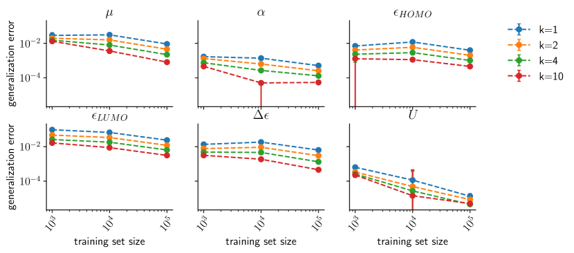
Figure 4: Estimated relative generalization error on the QM9 dataset for additional targets. Specifically, we show results for dipole moment $\mu$, isotropic polarizability $\alpha$, highest occupied molecular orbital energy $\epsilon_{HOMO}$, lowest occupied molecular orbital energy $\epsilon_{LUMO}$, HOMO-LUMO gap $\Delta\epsilon=\epsilon_{HOMO}-\epsilon_{LUMO}$, internal energy $U$ at 298.15K.

References

- [1] Anselm Blumer, A. Ehrenfeucht, David Haussler, and Manfred K. Warmuth. Learnability and the vapnik-chervonenkis dimension. J. ACM, 36(4):929–965, oct 1989.
- [2] Shai Shalev-Shwartz and Shai Ben-David. Understanding machine learning: From theory to algorithms. Cambridge university press, 2014.
- [3] Lauren B Wheelock, Stephen Malina, Jeffrey Gerold, and Sam Sinai. Forecasting labels under distribution-shift for machine-guided sequence design. In Machine Learning in Computational Biology, pages 166–180. PMLR, 2022.
- [4] Drew H Bryant, Ali Bashir, Sam Sinai, Nina K Jain, Pierce J Ogden, Patrick F Riley, George M Church, Lucy J Colwell, and Eric D Kelsic. Deep diversification of an aav capsid protein by machine learning. Nature Biotechnology, 39(6):691–696, 2021.
- [5] Vladimir Gligorijević, Daniel Berenberg, Stephen Ra, Andrew Watkins, Simon Kelow, Kyunghyun Cho, and Richard Bonneau. Function-guided protein design by deep manifold sampling. bioRxiv, pages 2021–12, 2021.
- [6] Jung-Eun Shin, Adam J Riesselman, Aaron W Kollasch, Conor McMahon, Elana Simon, Chris Sander, Aashish Manglik, Andrew C Kruse, and Debora S Marks. Protein design and variant prediction using autoregressive generative models. Nature communications, 12(1):2403, 2021.
- [7] Saleh Riahi, Jae Hyeon Lee, Shuai Wei, Robert Cost, Alessandro Masiero, Catherine Prades, Reza Olfati-Saber, Maria Wendt, Anna Park, Yu Qiu, and Yanfeng Zhou. Application of an integrated computational antibody engineering platform to design SARS-CoV-2 neutralizers. Antibody Therapeutics, 4(2):109–122, 06 2021.
- [8] Samuel Stanton, Wesley Maddox, Nate Gruver, Phillip Maffettone, Emily Delaney, Peyton Greenside, and Andrew Gordon Wilson. Accelerating bayesian optimization for biological sequence design with denoising autoencoders. In International Conference on Machine Learning, pages 20459–20478. PMLR, 2022.
- [9] Brajesh K Rai, James R Apgar, and Eric M Bennett. Low-data interpretable deep learning prediction of antibody viscosity using a biophysically meaningful representation. Scientific Reports, 13(1):2917, 2023.
- [10] Vladimir Vapnik, Esther Levin, and Yann Le Cun. Measuring the vc-dimension of a learning machine. Neural computation, 6(5):851–876, 1994.
- [11] Peter L Bartlett, Dylan J Foster, and Matus J Telgarsky. Spectrally-normalized margin bounds for neural networks. Advances in neural information processing systems, 30, 2017.
- [12] David A McAllester. Some pac-bayesian theorems. In Proceedings of the eleventh annual conference on Computational learning theory, pages 230–234, 1998.
- [13] John Shawe-Taylor and Robert C. Williamson. A pac analysis of a bayesian estimator. In Proceedings of the Tenth Annual Conference on Computational Learning Theory, COLT ’97, page 2–9, New York, NY, USA, 1997. Association for Computing Machinery.
- [14] Gintare Karolina Dziugaite and Daniel M Roy. Computing nonvacuous generalization bounds for deep (stochastic) neural networks with many more parameters than training data. arXiv preprint arXiv:1703.11008, 2017.
- [15] Behnam Neyshabur, Srinadh Bhojanapalli, and Nathan Srebro. A pac-bayesian approach to spectrally-normalized margin bounds for neural networks. In International Conference on Learning Representations, 2018.
- [16] Wenda Zhou, Victor Veitch, Morgane Austern, Ryan P. Adams, and Peter Orbanz. Non-vacuous generalization bounds at the imagenet scale: a PAC-bayesian compression approach. In International Conference on Learning Representations, 2019.
- [17] Roi Livni and Shay Moran. A limitation of the pac-bayes framework. In H. Larochelle, M. Ranzato, R. Hadsell, M.F. Balcan, and H. Lin, editors, Advances in Neural Information Processing Systems, volume 33, pages 20543–20553. Curran Associates, Inc., 2020.
- [18] Gintare Karolina Dziugaite, Kyle Hsu, Waseem Gharbieh, Gabriel Arpino, and Daniel Roy. On the role of data in pac-bayes bounds. In International Conference on Artificial Intelligence and Statistics, pages 604–612. PMLR, 2021.
- [19] Sanae Lotfi, Marc Finzi, Sanyam Kapoor, Andres Potapczynski, Micah Goldblum, and Andrew G Wilson. Pac-bayes compression bounds so tight that they can explain generalization. Advances in Neural Information Processing Systems, 35:31459–31473, 2022.
- [20] Huan Xu and Shie Mannor. Robustness and generalization. Machine learning, 86:391–423, 2012.
- [21] Jure Sokolić, Raja Giryes, Guillermo Sapiro, and Miguel RD Rodrigues. Robust large margin deep neural networks. IEEE Transactions on Signal Processing, 65(16):4265–4280, 2017.
- [22] Andreas Loukas, Marinos Poiitis, and Stefanie Jegelka. What training reveals about neural network complexity. Advances in Neural Information Processing Systems, 34:494–508, 2021.
- [23] Arthur Jacot, Franck Gabriel, and Clément Hongler. Neural tangent kernel: Convergence and generalization in neural networks. Advances in neural information processing systems, 31, 2018.
- [24] Olivier Bousquet and André Elisseeff. Stability and generalization. The Journal of Machine Learning Research, 2:499–526, 2002.
- [25] Moritz Hardt, Ben Recht, and Yoram Singer. Train faster, generalize better: Stability of stochastic gradient descent. In International Conference on Machine Learning, pages 1225–1234. PMLR, 2016.
- [26] Elad Hoffer, Itay Hubara, and Daniel Soudry. Train longer, generalize better: closing the generalization gap in large batch training of neural networks. In NIPS, 2017.
- [27] Ilja Kuzborskij and Christoph Lampert. Data-dependent stability of stochastic gradient descent. In International Conference on Machine Learning, pages 2815–2824. PMLR, 2018.
- [28] Nisha Chandramoorthy, Andreas Loukas, Khashayar Gatmiry, and Stefanie Jegelka. On the generalization of learning algorithms that do not converge. In Advances in Neural Information Processing Systems.
- [29] Chiyuan Zhang, Samy Bengio, Moritz Hardt, Benjamin Recht, and Oriol Vinyals. Understanding deep learning (still) requires rethinking generalization. Communications of the ACM, 64(3):107–115, 2021.
- [30] Chuan Guo, Geoff Pleiss, Yu Sun, and Kilian Q Weinberger. On calibration of modern neural networks. In International conference on machine learning, pages 1321–1330. PMLR, 2017.
- [31] Hao Song, Tom Diethe, Meelis Kull, and Peter Flach. Distribution calibration for regression. In Kamalika Chaudhuri and Ruslan Salakhutdinov, editors, Proceedings of the 36th International Conference on Machine Learning, volume 97 of Proceedings of Machine Learning Research, pages 5897–5906. PMLR, 09–15 Jun 2019.
- [32] Alexandru Niculescu-Mizil and Rich Caruana. Predicting good probabilities with supervised learning. In Proceedings of the 22nd international conference on Machine learning, pages 625–632, 2005.
- [33] Matteo Fontana, Gianluca Zeni, and Simone Vantini. Conformal prediction: a unified review of theory and new challenges. Bernoulli, 29(1):1–23, 2023.
- [34] Thomas M Cover and Joy A Thomas. Information theory and statistics. Elements of information theory, 1(1):279–335, 1991.
- [35] Zhenqin Wu, Bharath Ramsundar, Evan N Feinberg, Joseph Gomes, Caleb Geniesse, Aneesh S Pappu, Karl Leswing, and Vijay S Pande. Moleculenet. CoRR, abs/1703.00564, 2017.
- [36] Matthias Fey and Jan E. Lenssen. Fast graph representation learning with PyTorch Geometric. In ICLR Workshop on Representation Learning on Graphs and Manifolds, 2019.
- [37] Derek M Mason, Simon Friedensohn, Cédric R Weber, Christian Jordi, Bastian Wagner, Simon M Meng, Roy A Ehling, Lucia Bonati, Jan Dahinden, Pablo Gainza, et al. Optimization of therapeutic antibodies by predicting antigen specificity from antibody sequence via deep learning. Nature Biomedical Engineering, 5(6):600–612, 2021.
- [38] Jonathan Parkinson, Ryan Hard, and Wei Wang. The resp ai model accelerates the identification of tight-binding antibodies. Nature Communications, 14(1):454, 2023.