CertPri: Certifiable Prioritization for Deep Neural Networks via Movement Cost in Feature Space

Abstract

Deep neural networks (DNNs) have demonstrated their outperformance in various software systems, but also exhibit misbehavior and even result in irreversible disasters. Therefore, it is crucial to identify the misbehavior of DNN-based software and improve DNNs’ quality. Test input prioritization is one of the most appealing ways to guarantee DNNs’ quality, which prioritizes test inputs so that more bug-revealing inputs can be identified earlier with limited time and manual labeling efforts. However, the existing prioritization methods are still limited from three aspects: certifiability, effectiveness, and generalizability. To overcome the challenges, we propose CertPri, a test input prioritization technique designed based on a movement cost perspective of test inputs in DNNs’ feature space. CertPri differs from previous works in three key aspects: (1) certifiable - it provides a formal robustness guarantee for the movement cost; (2) effective - it leverages formally guaranteed movement costs to identify malicious bug-revealing inputs; and (3) generic - it can be applied to various tasks, data, models, and scenarios. Extensive evaluations across 2 tasks (i.e., classification and regression), 6 data forms, 4 model structures, and 2 scenarios (i.e., white-box and black-box) demonstrate CertPri’s superior performance. For instance, it significantly improves 53.97% prioritization effectiveness on average compared with baselines. Its robustness and generalizability are 1.41$\sim$2.00 times and 1.33$\sim$3.39 times that of baselines on average, respectively. The code of CertPri is open-sourced at https://anonymous.4open.science/r/CertPri.

I Introduction

Deep neural networks (DNNs) [1] have performed impressive success in many fields, including computer vision [2, 3, 4], natural language processing [5, 6], and software engineering [7, 8], etc. However, like traditional software systems, DNNs are also vulnerable in terms of quality and reliability [9, 10, 11, 12]. Meanwhile, these vulnerabilities could lead to serious losses such as a crash caused by a Google self-driving car [13], and even irreversible disasters such as the deadly car crash caused by the autopilots of Tesla [14] and Uber [15]. Therefore, it is crucial to detect the misbehavior of DNN-based software and ensure DNNs’ quality.

Much effort has been put into DNN-based software quality assurance [12, 16, 17, 18, 19, 20]. One of the most appealing methods is test input prioritization [21, 22], which prioritizes test inputs so that more bug-revealing inputs (e.g., misclassified inputs) can be identified earlier with limited time and manual labeling efforts. Moreover, these inputs facilitate the debugging of DNN-based software, which could improve DNNs’ quality [23, 24] and reduce their retraining cost [25]. There are several prioritization methods, mainly including four aspects, i.e., coverage-based [20, 12, 26], surprise-based [27, 22, 28], confidence-based [23, 25, 29], and mutation-based [24] methods. The first two methods prioritize test inputs based on DNNs’ neuron coverage and surprise-adequacy activation traces, respectively. Confidence-based methods identify bug-revealing inputs by measuring the classifier’s output probabilities. Mutation-based methods design a series of mutation operations, and then analyze the mutated output probabilities based on supervised learning. These methods make great progress in identifying bug-revealing inputs earlier, but they still suffer from the following problems.

First, the existing methods are empirically lacking formal guarantees, which results in vulnerability against malicious attacks, i.e., prioritizing bug-revealing inputs at the back when attacked. More specifically, taking neuron activation suppression as an optimization objective, the adversary could craft imperceptible adversarial perturbations [30, 31]. These bug-revealing inputs with perturbations will be prioritized at the back due to low neuron coverage or inadequate activation traces, i.e., coverage-based and surprise-based methods lose their effectiveness. Similarly, confidence-based methods fail to work when increasing the highest probability value [32, 33] by adding well-designed perturbations to inputs. Mutation-based methods include input mutation and model mutation, both of which are similar to data augmentation [34, 35] and network modification [36, 37], respectively. Once the mutation operations are leaked, the adversary can bypass these operations by crafting malicious bug-revealing inputs. Then, mutation-based methods will be invalid. Therefore, a formal robustness guarantee for certifiable prioritization is required.

Second, almost all methods either suffer from prioritization effectiveness or efficiency issues. For instance, coverage-based methods have been demonstrated to be ineffective and time-costly [23]. Surprise-based methods improve test input prioritization by utilizing more advanced metrics (e.g., surprise-adequacy and activation frequency), but are computationally expensive due to more parameter tuning. Confidence-based methods apply output probabilities to perform fast and lightweight prioritization, and their effectiveness is better than the previous two. However, once adversarial [32] or poisoned [38] inputs are injected into the test dataset, their effectiveness drops largely. Mutation-based test input prioritization, PRIMA [24], is the state-of-the-art (SOTA) method for DNNs, outperforming the confidence-based methods by an average of 10%, but with a time cost increase of more than 100 times. Moreover, PRIMA is a supervised prioritization method, i.e., its effectiveness is affected by training dataset size and category balance.

Third, most methods suffer from the generalizability issue, including the generalizability of tasks, data forms, model structures, and application scenarios. For instance, confidence-based methods rely on DNNs’ output probabilities, and thus may not be directly generalized to a regression task. Meanwhile, their prioritization effectiveness for sequential data form (e.g., text data [5]) has been demonstrated to drop by an average of 30% in the existing study [24]. Mutation-based methods could be generalized to various data and tasks, but specialized domain knowledge is required to design diverse data-specific (e.g., structured data [39] and graph data [40]) mutation strategies. Moreover, it is unclear whether their model mutation strategies can still perform well on other model structures, such as graph convolution network (GCN) [40]. Except for confidence-based methods, the other three types are all designed for white-box testing and need to acquire DNNs’ details. In black-box scenarios, these white-box methods will seriously degrade performance or even fail to work.

To overcome these challenges, our design goals are as follows: (1) we intend to take formal guarantee into account when designing a certifiable prioritization method; (2) we want the certifiability to serve prioritization effectiveness without degrading efficiency; (3) we plan to evaluate its generalizability.

One of the main contributions of DNNs is automatic feature extraction [1], which maps test inputs from the data space to the feature space. Based on the mapping ability, Zheng et al. [41] improved the robustness of DNNs by pushing the test input to the target position (i.e., class center) based on inverse perturbation. Further, we find that the inverse perturbation measures the movement cost of test inputs in feature space. Thus, we explore the variation in the movement cost of different test inputs and give an example as shown in Figure 1. We compute the movement cost (i.e., inverse perturbation based on infinite norm) of 5,000 test inputs from ImageNet [42] on a pre-trained VGG model [2]. We first divide test inputs into 10 groups according to the original prediction probability, and then calculate the movement cost of reaching a position with a higher probability. As shown in Figure 1, we find that there was a significant difference (p-value=2.38E-07 based on T-test) in the movement cost of correctly and incorrectly predicted test inputs, which can be considered for prioritization. However, the inverse perturbation [41] is obtained through iterative training, which is still empirical. To satisfy the certifiability requirement, we further derive a formal guarantee of the inverse perturbation with the Lipschitz continuity assumption [43].

According to the utility analysis and certifiability consideration, we design a certifiable prioritization technique, CertPri, which reduces the problem of measuring misbehavior probability to the problem of measuring the movement difficulty in feature space, i.e., the movement cost of the test inputs being close to or far from the class centers. Then, we compute the certifiable inverse perturbation based on the generalized extreme value theory (GEVT) [44]. Based on the formal robustness guarantee, CertPri is valid for identifying malicious bug-revealing inputs, as well as clean bug-revealing inputs, without degrading efficiency.

To compute the inverse perturbation, the model gradient is used [45]. Since DNNs are an end-to-end learning paradigm [46], the gradient can be directly computed when data and models are available in a white-box scenario. In a black-box scenario, the approximate gradient can be computed by gradient estimation [47]. Furthermore, to evaluate CertPri’s generalizability, we conduct extensive experiments on various tasks, data forms, data types, model structures, training and prioritization scenarios.

The main contributions are as follows.

• Through inverse perturbation analysis and measurement, we first implement a formal robustness guarantee for the movement cost, which provides a new perspective for measuring DNNs’ misbehavior probability.

• Based on the formal guarantee of movement costs, we propose an effective and efficient technique, CertPri, which leverages certifiability to facilitate the prioritization effectiveness.

• To evaluate CertPri’s generalizability, we conduct extensive experiments on various tasks, data, models and scenarios, the results of which show the superiority of CertPri compared with previous works.

• We publish CertPri as a self-contained open-source toolkit online for facilitating DNNs’ prioritization research.

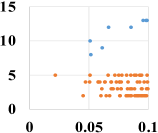
(a) (0,0.1)

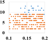
(b) [0.1,0.2)

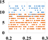
(c) [0.2,0.3)

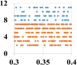
(d) [0.3,0.4)

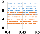
(e) [0.4,0.5)

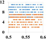
(f) [0.5,0.6)

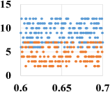
(g) [0.6,0.7)

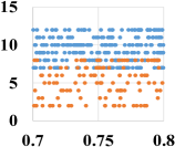
(h) [0.7,0.8)

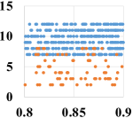
(i) [0.8,0.9)

(j) [0.9,1.0)

Figure 1: An example of movement cost for test inputs with different probability levels, where “$\bullet$” and “$\bullet$” represent correctly and incorrectly predicted test inputs, respectively. Subfigure (a) represents movement costs required for test inputs whose top-1 prediction probability belongs to (0, 0.1) to reach a position with a probability higher than 0.1, where the x-axis represents the original top-1 prediction probability and the y-axis represents the movement cost. We repeat 5 times and compute the average movement cost of each test input.

II Background

In this section, we first introduce the basic knowledge of DNNs, and then give the definitions of inverse perturbation.

II-A Deep Neural Networks

DNN consists of several layers, each of which contains a large number of neurons[1]. Generally, the basic tasks of DNNs include classification and regression. These tasks are accomplished by building models with various basic structures, such as fully connected network (FCN) [16], convolutional neural network (CNN) [2], long short-term memory (LSTM) [48], and GCN [40]. The classification and regression models are as follows.

The classification model predicts which class the test input belongs to. Suppose we have a $K$-class classifier $f^{C}:\mathbb{R}^{d}\to\mathbb{R}^{K}$. Given a test input $\bm{x}_{0}\in\mathbb{R}^{d}$, the classifier will output a vector of $K$ values normalized by softmax function [49], e.g., $\{f_{i}^{C}(\bm{x}_{0})|_{1\leq i\leq K}\}$, each of which represents the probability that $\bm{x}_{0}$ belongs to the $i$-th class, where $\{d,K\}\in\mathbb{Z}^{+}$ and $K\geq$2. $c(\bm{x}_{0})=\arg\max_{1\leq i\leq K}f_{i}^{C}(\bm{x}_{0})$ represents the predicted label of $\bm{x}_{0}$ and $f_{i}^{C}(\bm{x}_{0})\in(0,1)$.

The regression model describes a mapping between the test input and the output. Suppose we have a regression model $f^{R}:\mathbb{R}^{d_{1}}\to\mathbb{R}^{d_{2}}$. Given a test input $\bm{x}_{0}\in\mathbb{R}^{d_{1}}$, the regression model will output a vector with $d_{2}$ elements activated by linear or ReLU functions [50], e.g., $\{f_{i}^{R}(\bm{x}_{0})|_{1\leq i\leq d_{2}}\}$, each of which represents a fit to the ground-truth, where $\{d_{1},d_{2}\}\in\mathbb{Z}^{+}$. $r(\bm{x}_{0})=f^{R}(\bm{x}_{0})$ represents the fitted prediction output of $\bm{x}_{0}$ and $f_{i}^{R}(\bm{x}_{0})\in[\min_{r},\max_{r}]$.

II-B Definitions of Inverse Perturbation

We give definitions of inversely perturbed test input, minimum inverse perturbation, and lower bound.

Definition 1 (inversely perturbed test input). Given $\bm{x}_{0}$, we say $\bm{x}_{0}^{*}$ is an inversely perturbed test input of $\bm{x}_{0}$ with inverse perturbation $\bm{\mu}$ and $l_{p}$-norm $\Delta_{p}$ if $\bm{x}_{0}^{*}=\bm{x}_{0}+\bm{\mu}$ is moved to the target position and $\Delta_{p}=||\bm{\mu}||_{p}$. An inversely perturbed test input for a classifier is $\bm{x}_{0}^{*}\in\mathbb{R}^{d}$ that moves towards the class center of $c(\bm{x}_{0})$, where the class center is defined as $f_{center}^{C}(\bm{x}_{0})=\min\left\{f_{c}^{C}(\bm{x}_{0})\times[1+\log(1+f_{c}^{C}(\bm{x}_{0}))],1\right\}$. For a regression model, $\bm{x}_{0}^{*}\in\mathbb{R}^{d_{1}}$ moves from $r(\bm{x}_{0})$ to regression center, which is defined as $f^{R}_{i,+}(\bm{x}_{0})={\rm clip}_{\min_{r}}^{\max_{r}}\left(f_{i}^{R}(\bm{x}_{0})+|f_{i}^{R}(\bm{x}_{0})|\times\log\left[1+\tanh(f_{i}^{R}(\bm{x}_{0}))\right]\right)$.

Definition 2 (minimum inverse perturbation $\Delta_{p}^{\min}$ and its lower bound $\gamma_{L}$). Given a test input $\bm{x}_{0}$, the minimum $l_{p}$ inverse perturbation of $\bm{x}_{0}$, denoted as $\Delta_{p}^{\min}$, is defined as the smallest $\Delta_{p}$ over all inversely perturbed test inputs of $\bm{x}_{0}$. Suppose $\Delta_{p}^{\min}$ is the minimum inverse perturbation of $\bm{x}_{0}$. A lower bound of $\Delta_{p}^{\min}$, denoted by $\gamma_{L}$ where $\gamma_{L}\leq\Delta_{p}^{\min}$, is defined such that any inversely perturbed test inputs of $\bm{x}_{0}$ with $||\bm{\mu}||_{p}\leq\gamma_{L}$ will never reach the target position.

The lower bound of inverse perturbation measures the minimum movement cost for a test input to reach the target position (i.e., class center or regression center). $\gamma_{L}$ guarantees that the inversely perturbed test input will never move to the target position for inverse perturbation with $||\bm{\mu}||_{p}\leq\gamma_{L}$, certifying the movement cost of the test input. All the notations are summarized in Table I.

TABLE I: Definitions of Notations.

	Notations	Definitions
DNNs	$d$, $K$	dimensionality of test inputs, number of output classes
	$f^{C}:\mathbb{R}^{d}\to\mathbb{R}^{K}$	classification model
	$f^{C}_{i}(\bm{x}_{0})$	the $i$-th dimension output of the classification model
	$c(\bm{x}_{0})$	the predicted label of $\bm{x}_{0}$
	$d_{1}$, $d_{2}$	dimensionality of test inputs and outputs
	$f^{R}:\mathbb{R}^{d_{1}}\to\mathbb{R}^{d{2}}$	regression model
	$f^{R}_{i}(\bm{x}_{0})$	the $i$-th dimension output of the regression model
	$r(\bm{x}_{0})$	the fitted prediction output of $\bm{x}_{0}$
	$\max_{r}$, $\min_{r}$	maximum and minimum values of regression output domain
	$\bm{x}_{0}\in\mathbb{R}^{d}$, $\bm{x}_{0}\in\mathbb{R}^{d_{1}}$	original test input of classification and regression
Inverse Perturbation	$\bm{x}^{*}_{0}\in\mathbb{R}^{d}$, $\bm{x}^{*}_{0}\in\mathbb{R}^{d_{1}}$	inversely perturbed test input of classification and regression
	$\bm{\mu}\in\mathbb{R}^{d}$, $\bm{\mu}\in\mathbb{R}^{d_{1}}$	inverse perturbation of classification and regression
	$||\bm{\mu}||_{p}$	$l_{p}$-norm of inverse perturbation, $p\geq 1$
	$f^{C}_{center}(\bm{x}_{0})$, $f^{R}_{i,+}(\bm{x}_{0})$	class center and regression center
	$\min\{\cdot,\cdot\}$	returns the minimum element in the set
	${\rm clip}_{\min_{r}}^{\max_{r}}(\cdot)$	limit the input value to the range of ($\min_{r}$, $\max_{r}$)
	$\Delta_{p}^{min}$, $\gamma_{L}$	minimum inverse perturbation and its lower bound
	$L_{q}^{c}$, $L_{q}^{r}$	Lipschitz constant of classification and regression, $q\geq 1$

III CertPri Methodology

In this section, we present a technical description of CertPri. First, we discuss the prioritization feasibility based on a movement cost view. Then, we introduce CertPri, which provides a formal robustness guarantee based on the Lipschitz continuity assumption [43] and estimates the movement cost based on GEVT [45]. Finally, we prioritize inputs via movement costs.

III-A A Movement View in Feature Space

A well-trained DNN implements feature extraction through multiple hidden layers, each of which filters redundant features and amplifies key features during forward propagation [51]. If we regard the feature mapping of hidden layers as data movement in feature space, almost all test inputs are pushed towards the target position in forward propagation, while bug-revealing inputs fail to reach the target position at the end of forward propagation.

First, we investigate the movement process of test inputs in forward propagation. Taking a classifier based on a FCN with three hidden layers on MNIST [52] dataset as an example, the t-SNE [53] based distribution of test inputs in feature space is visualized in Figure 2. During the forward propagation as shown in Figure 2 (a), we observe that most test inputs directional approach the correct class, which realizes the right prediction. However, several test inputs move without direction leading to the DNN’s misbehavior (i.e., misclassification), which are the bug-revealing inputs that need to be identified. It is intuitively based on the feature purity theory of test inputs [23]. For a bug-revealing test input, it not only contains features of multiple classes, but the highest feature purity is close to the second highest one, and even the feature purity of each class is close. Thus, the movement of this test input in the forward propagation is directionless.

Then, we further analyze the movement cost of correctly and incorrectly predicted test inputs based on the inverse perturbation [41]. As shown in Figure 2 (b), the ground truth of $\bm{x}_{0}$ is II but is misclassified as III. As $\bm{x}_{0}$ proceeds along the gradient direction, its class center of III can be reached with low movement cost. However, correctly predicted test inputs require high movement cost to reach their class centers. It is consistent with the interpretation based on feature purity [23]. The incorrectly predicted test inputs improve the feature purity of the corresponding class after adding inverse perturbation, which turns random movement into directional movement in forward propagation. Therefore, only a low movement cost is required to reach the class center. The correctly predicted test inputs contain high feature purity, which keeps them stable in feature space. Thus, further movement requires a high cost. Note that the class center is given by Definition 1, which differs for each test input [41].

Based on the above analysis, we reduce the problem of measuring misbehavior probability of prioritization to the problem of measuring the movement cost in feature space. Thus, we prioritize test inputs by comparing their lower bounds of minimum movement cost to the target position. The test input never reaches the target position when the movement cost is less than the lower bound $\gamma_{L}$. However, $\gamma_{L}$ is not easy to find. Below we show how to derive a formal inverse perturbation guarantee of a test input with the Lipschitz continuity assumption [43].

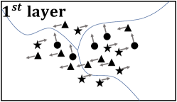
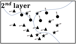
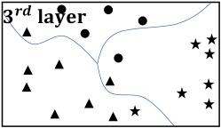
(a) The movement process of test inputs in forward propagation, where almost all test inputs move towards the corresponding class centers.

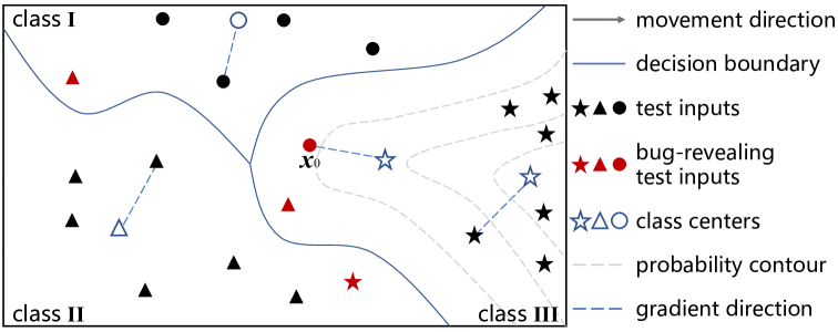
(b) The movement cost of test inputs in back propagation, where $\bm{x}_{0}$ is a misclassified test input, “probability contour” represents that test inputs on the same contour line have the same probability of belonging to the class, “gradient direction” is obtained by back propagation [54].

Figure 2: An example of t-SNE [53] based distribution visualization of test inputs in feature space. The classifier is a FCN with three hidden layers, the test inputs are handwritten digits of “0”(I), “1”(II) and “2”(III) from MNIST dataset [52].

III-B Formal Guarantees for Movement Cost

We first give the lemma about the Lipschitz continuity. According to the lemma, we then provide a formal guarantee for the lower bound of the inverse perturbation. Specifically, our analysis obtains a lower bound of $l_{p}$-norm minimum inverse perturbation $\gamma_{L}=\min\frac{f_{center}^{C}(\bm{x}_{0})-f_{c}^{C}(\bm{x}_{0})}{L_{q}^{c}}$ for a classifier and $\gamma_{L}\!=\!\min\frac{\sum_{i}|f_{i,+}^{R}(\bm{x}_{0})-f_{i}^{R}(\bm{x}_{0})|}{d_{2}\times L_{q}^{r}}$ for a regression model.

Lemma 1 (Norms and corresponding Lipschitz constants [43]). Let $D\subset\mathbb{R}^{d}$ be a convex bounded closed set and let $h(\bm{x}):S\to\mathbb{R}$ be a continuously differentiable function on an open set containing $D$. For a Lipschitz function $h(\bm{x})$ with Lipschitz constant $L_{q}$, the inequality $|h(\bm{a})-h(\bm{b})|\leq L_{q}||\bm{a}-\bm{b}||_{p}$ holds for any $\{\bm{a},\bm{b}\}\in D$, where $L_{q}=\max\{||\nabla_{\bm{x}}h(\bm{x})||_{q}:\bm{x}\in D\}$, $\nabla_{\bm{x}}h(\bm{x})=(\frac{\partial h}{\partial\bm{x}_{1}},...,\frac{\partial h}{\partial\bm{x}_{d}})$ is the gradient of $h(\bm{x})$, $\frac{1}{p}+\frac{1}{q}=1$ and $1\leq\{p,q\}\leq\infty$.

Theorem 1 (Formal guarantee on lower bound $\gamma_{L}$ of inverse perturbation for classification model). Let $\bm{x}_{0}\in\mathbb{R}^{d}$ and $f^{C}:\mathbb{R}^{d}\to\mathbb{R}^{K}$ be a $K$-class classifier with continuously differentiable components. For all $\bm{\mu}\in\mathbb{R}^{d}$ with $||\bm{\mu}||_{p}\leq\min\frac{f_{center}^{C}(\bm{x}_{0})-f_{c}^{C}(\bm{x}_{0})}{L_{q}^{c}}$, $f_{c}^{C}(\bm{x}_{0}+\bm{\mu})=f_{center}^{C}(\bm{x}_{0})$ holds with $\frac{1}{p}+\frac{1}{q}=1$, $1\leq\{p,q\}\leq\infty$ and $L_{q}^{c}$ is the Lipschitz constant for the function $f_{center}^{C}(\bm{x})-f_{c}^{C}(\bm{x})$ in $l_{p}$-norm. In other word, $\gamma_{L}=\min\frac{f_{center}^{C}(\bm{x}_{0})-f_{c}^{C}(\bm{x}_{0})}{L_{q}^{c}}$ is a lower bound of minimum inverse perturbation for moving to the class center.

Proof. According to Lemma 1, the assumption that the function $h(\bm{x}):=f_{center}^{C}(\bm{x})-f_{c}^{C}(\bm{x})$ is Lipschitz continuous with Lipschitz constant $L_{q}^{c}$ gives:

$$|h(\bm{a})-h(\bm{b})|\leq L_{q}^{c}||\bm{a}-\bm{b}||_{p}.$$ (1)

Let $\bm{a}=\bm{x}_{0}+\bm{\mu}$ and $\bm{b}=\bm{x}_{0}$, we get:

$$|h(\bm{x}_{0}+\bm{\mu})-h(\bm{x}_{0})|\leq L_{q}^{c}||\bm{\mu}||_{p},$$ (2)

which can be rearranged by removing the absolute symbol:

$$\begin{array}[]{ll}&\!\!-L_{q}^{c}||\bm{\mu}||_{p}\leq h(\bm{x}_{0}+\bm{\mu})-h(\bm{x}_{0})\leq L_{q}^{c}||\bm{\mu}||_{p},\\ \!\!\!\Rightarrow\!\!&\!\!h(\bm{x}_{0})-L_{q}^{c}||\bm{\mu}||_{p}\leq h(\bm{x}_{0}+\bm{\mu})\leq h(\bm{x}_{0})+L_{q}^{c}||\bm{\mu}||_{p}.\end{array}$$ (3)

When $h(\bm{x}_{0}+\bm{\mu})\!\!=\!\!0$, the inversely perturbed test input is moved to the class center. As represented by Equation (3), $h(\bm{x}_{0})-L_{q}^{c}||\bm{\mu}||_{p}$ is the lower bound of $h(\bm{x}_{0}+\bm{\mu})$. If $h(\bm{x}_{0})-L_{q}^{c}||\bm{\mu}||_{p}\geq 0$ for sufficiently small inverse perturbation $||\bm{\mu}||_{p}$, the inversely perturbed input cannot reach the class center, i.e.,

$$\begin{array}[]{ll}\!\!\!h(\bm{x}_{0})-L_{q}^{c}||\bm{\mu}||_{p}\geq 0&\!\!\Rightarrow||\bm{\mu}||_{p}\leq\frac{h(\bm{x}_{0})}{L_{q}^{c}}\\ &\!\!\Rightarrow||\bm{\mu}||_{p}\leq\frac{f_{center}^{C}(\bm{x}_{0})-f_{c}^{C}(\bm{x}_{0})}{L_{q}^{c}}.\end{array}$$ (4)

To realize $f_{c}^{C}(\bm{x}_{0}+\bm{\mu})=f_{center}^{C}(\bm{x}_{0})$ we take the minimum of the bound on $||\bm{\mu}||_{p}$, i.e., the test input will never move to the class center when $||\bm{\mu}||_{p}\leq\min\frac{f_{center}^{C}(\bm{x}_{0})-f_{c}^{C}(\bm{x}_{0})}{L_{q}^{c}}$.

Theorem 2 (Formal guarantee on lower bound $\gamma_{L}$ of inverse perturbation for regression model). Let $\bm{x}_{0}\in\mathbb{R}^{d_{1}}$ and $f^{R}:\mathbb{R}^{d_{1}}\to\mathbb{R}^{d_{2}}$ be a regression model with continuously differentiable components. For all $\bm{\mu}\in\mathbb{R}^{d_{1}}$ with $||\bm{\mu}||_{p}\leq\min\frac{\sum_{i}|f_{i,+}^{R}(\bm{x}_{0})-f_{i}^{R}(\bm{x}_{0})|}{d_{2}\times L_{q}^{r}}$, $\frac{1}{d_{2}}\sum|r(\bm{x}_{0}+\bm{\mu})-r(\bm{x}_{0})|\leq\delta$ holds with $\frac{1}{p}+\frac{1}{q}=1$, $1\leq\{p,q\}\leq\infty$ and $L_{q}^{r}$ is the Lipschitz constant for the function $\frac{\sum_{i}|f_{i,+}^{R}(\bm{x})-f_{i}^{R}(\bm{x})|}{d_{2}}$ in $l_{p}$-norm. In other word, $\gamma_{L}=\min\frac{\sum_{i}|f_{i,+}^{R}(\bm{x}_{0})-f_{i}^{R}(\bm{x}_{0})|}{d_{2}\times L_{q}^{r}}$ is a lower bound of minimum inverse perturbation. The complete proof is deferred to https://anonymous.4open.science/r/CertPri/SupplementaryMaterials.pdf.

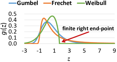
(a) PDF

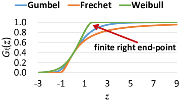
(b) CDF

Figure 3: Curves of PDF and CDF for different distributions, where $\xi=0$ for Gumbel, $\xi=0.6$ for Fr$\rm{\acute{e}}$chet and $\xi=-0.6$ for Weibull, $u=0$, $\sigma=1$.

III-C Movement Cost Estimation via GEVT

The formal guarantees give that $\gamma_{L}$ is related to $h(\bm{x}_{0})$ and its Lipschitz constant $L_{q}$, where $L_{q}=\max\{||\nabla_{\bm{x}}h(\bm{x})||_{q}:\bm{x}\in B_{p}(\bm{x}_{0},\mathcal{R})\}$, $B_{p}(\bm{x}_{0},\mathcal{R}):=\{\bm{x}|_{||\bm{x}-\bm{x}{0}||_{p}\leq\mathcal{R}}\}$ is a hyper-ball with center $\bm{x}_{0}$ and radius $\mathcal{R}$. The value of $h(\bm{x}_{0})$ is easily accessible at the model output. Thus, we show how to get $\max||\nabla_{\bm{x}}h(\bm{x})||_{q}$.

For a random variable sequence $\{\bm{x}_{0}^{(j)}\}$ sampled from $B_{p}(\bm{x}_{0},\mathcal{R})$, its corresponding gradient norm can be regarded as a new random variable sequence $\{||\nabla_{\bm{x}}h(\bm{x}_{0}^{(j)})||_{q}\}$ characterized by a cumulative distribution function (CDF) [45]. Therefore, we estimate $\max||\nabla_{\bm{x}}h(\bm{x}_{0}^{(j)})||_{q}$ with a small number of samples based on GEVT, which ensures that the maximum value of a random variable sequence can only follow one of the three extreme value distributions [44]. The CDF of $||\nabla_{\bm{x}}h(\bm{x}_{0}^{(j)})||_{q}$ is as follows:

$$G_{\xi}(\bm{z})=\exp\left(-(1+\xi\bm{z})^{-\frac{1}{\xi}}\right),$$ (5)

where $1\!+\!\xi\bm{z}>0$, $\bm{z}=\frac{||\nabla_{\bm{x}}h(\bm{x}_{0}^{(j)})||_{q}-u}{\sigma}$, $\xi\in\mathbb{R}$ is a extreme value index, $u\in\mathbb{R}$ and $\sigma\in\mathbb{R}^{+}$ are the expectation and variance. The parameters $u$, $\sigma$ and $\xi$ determine the location, scale and shape of $G_{\xi}(\bm{z})$, respectively. $G_{\xi}(\bm{z})$ belongs to either the Gumbel ($\xi=0$), Fr$\rm{\acute{e}}$chet ($\xi>0$) or Weibull ($\xi<0$) distributions.

We plot curves of probability density function (PDF) and its CDF for different extreme value distributions in Figure 3, where PDF (denoted as $g_{\xi}(\bm{z})$) is the differential of CDF. The Weibull distribution shows an interesting property in Figure 3, i.e., a finite right end-point (denoted as $-\frac{1}{\xi}$), which limits the upper bound of the distribution. Therefore, we adopt the Weibull to describe the gradient norm distribution, where the right end-point is the estimation of $\max||\nabla_{\bm{x}}h(\bm{x})||_{q}$.

Algorithm 1: CertPri.
	Input: Test inputs $\{\bm{x}_{i}\}$, $i\in\{0,1,...,N\!-\!1\}$, a classification model $f^{C}$, the sampling radius $\mathcal{R}$, batch size $N_{b}$, number of random samples per batch $N_{{rsb}}$, norm value $p$.
	Output: The prioritization index $\Omega$.
1	$h(\bm{x}):=f^{C}_{center}(\bm{x})-f^{C}_{c}(\bm{x})$, $q=\frac{p}{p-1}$, $\Gamma=\{\emptyset\}$.
2	For $i=0:N\!-\!1$ do
3	$S_{\nabla}=\{\emptyset\}$.
4	For $j=0:N_{b}\!-\!1$ do
5	For $k=0:N_{rsb}\!-\!1$ do
6	$g_{i,j,k}\!=\!||\nabla_{\bm{x}}h(\bm{x}_{i}^{(j,k)})||_{q}$.
7	End For
8	$g_{i,j}^{\max}=\max\{g_{i,j,k}\}$ and $S_{\nabla}=S_{\nabla}\cup\{g_{i,j}^{\max}\}$.
9	End For
10	Estimate $\hat{\xi}$ of Weibull distribution on $S_{\nabla}$.
11	$\gamma_{L}=\frac{h(\bm{x}_{i})}{-1/\hat{\xi}}$ and $\Gamma=\Gamma\cup{\gamma_{L}}$.
12	End For
13	$\Omega$ $\leftarrow$ return the index of $\Gamma$ in ascending order.

III-D Prioritization through Movement Cost

Based on the movement cost perspective in Section III-A, we can conclude that a test input with a small value of $\gamma_{L}$ should be prioritized at the front. Therefore, we compute the $\gamma_{L}$ value of each test input, and then prioritize these inputs according to their $\gamma_{L}$ values from small to large. Algorithm 1 shows the details of CertPri by taking the classification model as an example. We first establish the gradient norm distribution of a test input by randomly sampling in the hyper-ball (the loop from lines 4 to 9). Then, we estimate the location of the maximum gradient norm based on the Weibull distribution and compute the lower bound of the movement cost based on Theorem 1 (lines 10 and 11). Finally, we repeat the above operations for each test input (the loop from lines 2 to 12) and prioritize them according to the ascending result of their $\gamma_{L}$ values (line 13). Note that for algorithmic illustration, we only compute one $g_{i,j}^{\max}$ (line 8) for each iteration. To implement the best efficiency of GPU, we usually evaluate these values in batches, and thus a batch of $g_{i,j}^{\max}$ can be returned.

Furthermore, we can easily generalize CertPri to a regression model through replacing the $h(\bm{x})$ function at line 1 with $h(\bm{x}):=\frac{\sum_{i}|f_{i,+}^{R}(\bm{x})-f_{i}^{R}(\bm{x})|}{d_{2}}$ based on Theorem 2. Besides, we can extend CertPri to a black-box scenario based on the gradient estimation [47].

IV Experimental Setting

In this section, we introduce the experimental setup, including the subjects we considered, the baselines we compared with, the measurements we used, and the implementation details we conducted.

IV-A Subjects

We adopt 50 pairs of datasets and models as subjects, as shown in Table II. To sufficiently evaluate CertPri’s effectiveness, efficiency, robustness, generalizability and guidance, we carefully consider the diversity of subjects from six dimensions. To our best knowledge, this is the most large-scale and diverse study in the field.

(1) Various tasks of deep models. We employ both classification models (ID: 1-32, 37-45, 47-49) and regression models (ID: 33-36, 46, 50). The number of classes ranges from 2 to 1,000 across all the classification tasks.

(2) Various data forms of test inputs. We consider six data forms of test inputs from 14 datasets, including image, text, speech, signal, graph, and structured data. Specifically, we collect 6 image datasets, i.e., CIFAR10 [55] (a 10-class ubiquitous object dataset with 32$\times$32 pixels), ImageNet [42] (a 1,000-class object recognition benchmark with 224$\times$224 pixels), DrivingSA [56] (a steer angle regression dataset for autonomous driving from Udacity with 128$\times$128 pixels), Fashion-MNIST (FMNIST) [57] (a 10-class dataset of Zalando’s article images with 28$\times$28 pixels), Ants_Bees (a binary insect dataset containing ants and bees for transfer learning with 224$\times$224 pixels), and Cats_Dogs (a binary pet dataset containing cats and dogs for transfer learning with 224$\times$224 pixels), 2 text datasets, i.e., IMDB [58] (a binary movie review sentiment dataset encoded as a list of word indexes) and Reuters (a 46-class newswire dataset), one speech dataset, i.e., VCTK10 (a 10-class dataset of ten English speakers with various accents selected from VCTK Corpus with 601$\times$64 phonemes), one signal dataset, i.e., RML8PSK [59] (a signal regression dataset modulated by 8PSK from RadioML 2016.10a with 127$\times$2 points as input and 2 points as output), one graph dataset, i.e., Cora [60] (a 7-class citation network of scientific publications with 5,429 links), and 3 structured datasets, i.e., Adult [61] (a binary income dataset with 13-dimensional attributes), COMPAS (a binary crime prediction dataset with 400-dimensional attributes), and Boston (a housing price regression dataset with 13-dimensional input and 1-dimensional output).

TABLE II: Basic information of subjects.

ID	Datasets	Models	Struc.	#Inputs	Types	Forms	Tasks	Scenarios
1	CIFAR10	ResNet50	CNN	10,000	original	image	C	N+W
2	CIFAR10	ResNet50	CNN	10,000	original	image	C	N+B
3	CIFAR10	ResNet50	CNN	10,000	+BIM	image	C	N+W
4	CIFAR10	ResNet50	CNN	10,000	+C&W	image	C	N+W
5	CIFAR10	ResNet50	CNN	10,000	+FineFool	image	C	N+W
6	CIFAR10	ResNet50	CNN	10,000	+AdapS	image	C	N+W
7	CIFAR10	ResNet50	CNN	10,000	+AdapC	image	C	N+W
8	CIFAR10	ResNet50	CNN	10,000	+AdapM	image	C	N+W
9	CIFAR10	VGG16	CNN	10,000	original	image	C	N+W
10	CIFAR10	VGG16	CNN	10,000	original	image	C	N+B
11	CIFAR10	VGG16	CNN	10,000	+BIM	image	C	N+W
12	CIFAR10	VGG16	CNN	10,000	+C&W	image	C	N+W
13	CIFAR10	VGG16	CNN	10,000	+FineFool	image	C	N+W
14	CIFAR10	VGG16	CNN	10,000	+AdapS	image	C	N+W
15	CIFAR10	VGG16	CNN	10,000	+AdapC	image	C	N+W
16	CIFAR10	VGG16	CNN	10,000	+AdapM	image	C	N+W
17	ImageNet	ResNet101	CNN	5,000	original	image	C	N+W
18	ImageNet	ResNet101	CNN	5,000	original	image	C	N+B
19	ImageNet	ResNet101	CNN	5,000	+BIM	image	C	N+W
20	ImageNet	ResNet101	CNN	5,000	+C&W	image	C	N+W
21	ImageNet	ResNet101	CNN	5,000	+FineFool	image	C	N+W
22	ImageNet	ResNet101	CNN	5,000	+AdapS	image	C	N+W
23	ImageNet	ResNet101	CNN	5,000	+AdapC	image	C	N+W
24	ImageNet	ResNet101	CNN	5,000	+AdapM	image	C	N+W
25	ImageNet	VGG19	CNN	5,000	original	image	C	N+W
26	ImageNet	VGG19	CNN	5,000	original	image	C	N+B
27	ImageNet	VGG19	CNN	5,000	+BIM	image	C	N+W
28	ImageNet	VGG19	CNN	5,000	+C&W	image	C	N+W
29	ImageNet	VGG19	CNN	5,000	+FineFool	image	C	N+W
30	ImageNet	VGG19	CNN	5,000	+AdapS	image	C	N+W
31	ImageNet	VGG19	CNN	5,000	+AdapC	image	C	N+W
32	ImageNet	VGG19	CNN	5,000	+AdapM	image	C	N+W
33	DrivingSA	VGG19-AD	CNN	5,279	original	image	R	N+W
34	DrivingSA	VGG19-AD	CNN	5,279	original	image	R	N+B
35	DrivingSA	VGG19-AD	CNN	5,279	patch	image	R	N+W
36	DrivingSA	VGG19-AD	CNN	5,279	saturation	image	R	N+W
37	FMNIST	AlexNet	CNN	10,000	original	image	C	N+W
38	FMNIST_P	AlexNet-P	CNN	10,000	original	image	C	P+W
39	Ants_Bees	VGG16-AB	CNN	153	original	image	C	T+W
40	Cats_Dogs	VGG19-CD	CNN	5,000	original	image	C	T+W
41	IMDB	CNN-I	CNN	10,000	original	text	C	N+W
42	IMDB	LSTM-I	LSTM	10,000	original	text	C	N+W
43	Reuters	CNN-R	CNN	2,246	original	text	C	N+W
44	Reuters	LSTM-R	LSTM	2,246	original	text	C	N+W
45	VCTK10	LSTM-V	LSTM	400	original	speech	C	N+W
46	RML8PSK	LSTM-RML	LSTM	312	original	signal	R	N+W
47	Cora	GCN-C	GCN	1,000	original	graph	C	N+W
48	Adult	LFCN-A	FCN	10,000	original	structured	C	N+W
49	COMPAS	HFCN-C	FCN	1,000	original	structured	C	N+W
50	Boston	FCN-B	FCN	102	original	structured	R	N+W
$\bullet$ where “C” and “R” represent classification/regression tasks. “N”, “P” and “T” represent normal training,
poisoning and transfer learning scenarios. “W” and “B” represent white/black-box prioritization scenarios.

(3) Various data types of test inputs. We mainly consider three data types, including original test inputs, adversarial test inputs, and adaptive attacked test inputs. For adversarial test inputs, we perform three widely-used adversarial attacks (i.e., basic iterative method (BIM) [62], Carlini & Wagner (C&W) [63] and FineFool [64]) to generate the same number of adversarial examples as the corresponding original test inputs for CIFAR10 and ImageNet, respectively. Then, following previous works [23, 24], we construct an adversarial test input set for each of the two datasets under each adversarial attack through randomly selecting half of the original test inputs and half of the adversarial examples, represented as “+BIM”, “+C&W”, “+FineFool”. For adaptive attacked test inputs, we follow the strategy introduced in Section I to produce them. Regarding the surprise-based method [28], we consider two objectives, flipping the labels of test inputs, and reducing their surprise (i.e., the activation difference between test inputs and the training inputs), which can be conducted by MAG-GAN [32]. Regarding confidence-based methods [23, 25], we first flip the labels of test inputs based on BIM [62], and then increase their highest probability value (up to 0.99 for CIFAR10 and 0.90 for ImageNet) by continuously adding perturbations. Regarding the mutation-based method [24], we first break its ranking model by adding noise to the extracted features, and then add perturbations to the test inputs based on back propagation [54] to generate noisy features. Finally, we construct an adaptive attacked test input set for each of the two datasets under each adaptive attack through randomly selecting half of the original test inputs and half of the adaptive attacked examples, represented as “+AdapS”, “+AdapC”, “+AdapM”. When crafting adversarial or adaptive attacked test inputs, we assume that the adversary knows the prioritization details.

Additionally, regarding VGG19-AD model, we implement three test input types respectively, i.e., the original one, the patched test inputs (randomly blocking 10% of pixels for each test input), and the saturation-modified test inputs (modifying the intensities of saturation channel [65] for each test input).

(4) Various structures of deep models. We employ CNN (ID: 1-41, 43), LSTM (ID: 42, 44-46), GCN (ID: 47) and FCN (ID: 48-50). The number of layers ranges from 3 to 101 across all models.

(5) Various training scenarios. We set up three training scenarios, including normal training, poisoning and transfer learning. For the poisoning scenario, we first craft a poisoned training set on FMNIST dataset, denoted as “FMNIST_P”, where the poisoning method is DeepPoison [66], the source label and poisoned label are “Pullover” and “Coat”, respectively. For the transfer learning scenario, we deploy the source domain as ImageNet with 1,000-class and the target domain as insect images or pet images with 2-class.

(6) Various prioritization scenarios. We set up two prioritization scenarios, including white-box and black-box. All details of the model and test inputs are available and used for prioritization in the white-box scenario (ID: 1, 3-9, 11-17, 19-25, 27-33, 35-50), while only model outputs and test inputs are available in the black-box scenario (ID: 2, 10, 18, 26, 34).

TABLE III: Application scope of prioritization methods.

Methods	Classification	Regression	White-bok	Black-box
LSA	✓	✓	✓	✕
DSA	✓	✕	✓	✕
MCP	✓	✕	✓	✓
DeepGini	✓	✕	✓	✓
PRIMA	✓	✓	✓	✓​​​$\backprime$
CertPri	✓	✓	✓	✓

IV-B Baselines

We consider five baselines, i.e., likelihood-based surprise adequacy (LSA) [28], distance-based surprise adequacy (DSA) [28], multiple-boundary clustering and prioritization (MCP) [25], DeepGini [23] and PRIMA [24]. LSA and DSA are surprise-based methods. MCP and DeepGini are efficient confidence-based methods for lightweight prioritization. PRIMA is an effective mutation-based method with the SOTA performance. The application scope of each method is shown in Table III, where “✓​​​$\backprime$ ” means PRIMA can only perform input mutation in the black-box scenario. Note that coverage-based methods have been shown to be significantly less effective [23] and thus are omitted. All baselines are configured according to the best performance setting reported in the respective papers.

TABLE IV: Overall comparison results across all subjects, measured based on average RAUC and its improvement, where “C” and “R” represent classification and regression, “n/a” means not applicable in theory.

Tasks	Methods	Average $\pm$ Standard Deviation RAUC-					Improvement of CertPri in RAUC-
		100	200	300	500	All	100	200	300	500	All
C	LSA	0.4401$\pm$0.2076	0.3950$\pm$0.2380	0.3980$\pm$0.2313	0.3813$\pm$0.2481	0.5851$\pm$0.1414	86.43%	106.30%	99.14%	102.36%	54.48%
	DSA	0.4688$\pm$0.2267	0.4461$\pm$0.2340	0.4527$\pm$0.2454	0.4265$\pm$0.2398	0.5926$\pm$0.1473	75.03%	82.67%	75.07%	80.93%	52.55%
	MCP	0.4464$\pm$0.2162	0.4721$\pm$0.2244	0.4830$\pm$0.2301	0.4885$\pm$0.2169	0.6776$\pm$0.1553	83.73%	72.61%	64.10%	57.96%	33.40%
	DeepGini	0.6150$\pm$0.2045	0.5914$\pm$0.2075	0.5914$\pm$0.2117	0.5766$\pm$0.2072	0.7293$\pm$0.1784	33.42%	37.79%	34.02%	33.82%	23.94%
	PRIMA	0.6794$\pm$0.2174	0.6700$\pm$0.2043	0.6698$\pm$0.2125	0.6633$\pm$0.2096	0.7666$\pm$0.1683	20.78%	21.61%	18.34%	16.34%	17.92%
	CertPri	0.8205$\pm$0.1126	0.8148$\pm$0.1011	0.7926$\pm$0.1123	0.7717$\pm$0.1205	0.9040$\pm$0.0517	n/a	n/a	n/a	n/a	n/a
R	LSA	0.4288$\pm$0.1357	0.3837$\pm$0.0328	0.4570$\pm$0.0974	0.4163$\pm$0.0483	0.6607$\pm$0.0216	90.18%	113.56%	80.72%	98.03%	30.15%
	PRIMA	0.7164$\pm$0.1590	0.6992$\pm$0.1747	0.6910$\pm$0.1847	0.6728$\pm$0.2033	0.7263$\pm$0.1607	13.83%	17.22%	19.51%	22.54%	18.39%
	CertPri	0.8154$\pm$0.0225	0.8195$\pm$0.0161	0.8258$\pm$0.0228	0.8244$\pm$0.0188	0.8599$\pm$0.0150	n/a	n/a	n/a	n/a	n/a

IV-C Measurements

We investigate CertPri’s prioritization performance from five aspects, including prioritization effectiveness, efficiency, robustness, generalizability and guidance.

(1) We evaluate the effectiveness of CertPri through the ratio of the area under curve (RAUC), which transforms the prioritization result to a curve [24], defined as follows for classification tasks:

$$\footnotesize\!\!\!\!{\rm RAUC}\!=\!\frac{\sum_{i=1}^{N}n_{i}}{N\!\!\times\!\!N^{\prime}\!+\frac{N^{\prime}\!-N^{\prime 2}}{2}},{\rm~{}where}~{}n_{i}\!=\!\left\{\begin{array}[]{l}\!\!\!n_{i\textrm{-}1}\!+\!1,~{}c(\bm{x}_{i}){\rm~{}is~{}correct}\\ \!\!\!n_{i\textrm{-}1},~{}{\rm otherwise}\end{array}\right.\!\!\!\!,$$ (6)

where $N$ and $N^{\prime}$ are the number of prioritized test inputs and bug-revealing inputs, $i\geq 1$ and $n_{0}\!=\!0$. In other words, the numerator and denominator represent the area under curve of the prioritization method and the ideal prioritization, respectively.

For regression tasks, RAUC is calculated based on the mean-square error (MSE) of prediction, as follows:

$$\footnotesize{\rm RAUC}=\frac{\sum_{i=1}^{N}m_{i}}{\sum_{j=1}^{N}M_{j}},~{}{\rm where}\left\{\begin{array}[]{l}m_{i}=m_{i\textrm{-}1}+{\rm MSE}\left(f^{R}(\bm{x}_{i})\right)\\ M_{j}\!=\!M_{j\textrm{-}1}+{\rm MSE}\left(f^{R}(\bm{x}_{j})\right)\end{array}\right.\!\!\!\!,$$ (7)

where $m_{i}$ and $M_{j}$ represent the accumulated MSE between the predicted results and the ground-truth of the prioritization method and the ideal prioritization, respectively. $i,j\geq 1$, $m_{0}\!=\!M_{0}\!=\!0$. Moreover, we follow the setup of Wang et al. [24], using RAUC-100, RAUC-200, RAUC-300, RAUC-500 and RAUC-all as fine-grained metrics, i.e. $N$=100, 200, 300, 500 and all. Larger RAUC is better.

(2) We evaluate the prioritization efficiency of CertPri through prioritization speed, i.e., the time cost of prioritize 1,000 test inputs (#seconds/1,000 Inputs). Smaller is better.

(3) We evaluate the prioritization robustness of CertPri through RAUC stability, denoted as RobR. Larger RobR is better, as follows:

$$\footnotesize\rm RobR=\frac{~{}~{}RAUC\textrm{-}all~{}of~{}adaptive~{}attacked~{}test~{}inputs~{}~{}}{RAUC\textrm{-}all~{}of~{}original~{}test~{}inputs}\times 100\%.$$ (8)

(4) We evaluate the prioritization generalizability of CertPri based on reward value, denoted as GenRew, as follows:

$$\small{\rm GenRew}=\frac{1}{N_{rep}\times N_{sub}}\sum_{i=1}^{N_{rep}}\sum_{j=1}^{N_{sub}}\frac{n_{pm}-k_{i,j}+1}{n_{pm}},$$ (9)

where $N_{sub}$ represents the number of selected subjects, $N_{rep}\!\!=\!\!5$ and $n_{pm}\!\!=\!\!6$ are the number of repetitions and prioritization methods in our experiments, respectively. $k_{i,j}\in\{1,2,...,n_{pm}\}$ represents that the method ranks in the $k$-th position in descending order of RAUC-all for the $j$-th subject at the $i$-th experimental repetition. GenRew $\in[\frac{1}{n_{pm}},1]$. Lager GenRew is better.

(5) We evaluate the prioritization guidance from two aspects: performance and robustness improvements for DNNs. The former subtracts the accuracy of original model from that of retrained model, while the latter subtracts the attack success rate [32] of retrained model from that of original model.

IV-D Implementation Details

To fairly study the performance of the baselines and CertPri, our experiments have the following settings. (1) Hyperparameter settings based on the double-minimum strategy: we conduct a preliminary study based on a small dataset, and find that $N_{b}$¿3, $N_{rsb}$¿5 and $0.02\max(\bm{x})$¡$\mathcal{R}$¡$0.05\max(\bm{x})$ for Algorithm 1 are effective in general. To guarantee CertPri’s effectiveness, we follow the double-minimum strategy, i.e., $N_{b}$=6, $N_{rsb}$=10, $\mathcal{R}$=0.04$\max(\bm{x})$, $p$=2 for Algorithm 1. (2) Model training: we download and use pretrained models on ImageNet. For other datasets, we train appropriate models as follows. The learning rate ranges from 1E-04 to 1E-02, the optimizer is Adam, training:validation:test = 7:1:2, and an early stop strategy is used to avoid overfitting. (3) Preprocessing: we fill in missing data points based on the mean value. There is no specific mutation strategy provided in PRIMA [24] for speech, signal, graph data forms and GCN model, thus we derive it from the existing mutation operations. (4) Data recording: we repeat the experiment 5 times and record about 9,000 raw data.

We conduct all the experiments on a server with one Intel i7-7700K CPU running at 4.20 GHz, 64 GB DDR4 memory, 4 TB HDD and one TITAN Xp 12 GB GPU card.

V Experimental Results and Analysis

We evaluate CertPri through answering the following research questions (RQ).
RQ1. Effectiveness: How effective is CertPri?
RQ2. Efficiency: How efficient is CertPri.?
RQ3. Robustness: How robust is CertPri?
RQ4. Generalizability: How generic is CertPri?
RQ5. Guidance: Can CertPri guide the retraining of DNNs?

V-A Effectiveness (RQ1)

How effective is CertPri in prioritizing test inputs?

When reporting the results, we focus on the effectiveness of the following aspects: overall, data forms, data types, training scenarios, and prioritization scenarios. The evaluation results are shown in Tables IV, V, VI, VII, VIII and IX.

TABLE V: The p-value of T-test for average RAUC between CertPri and each baseline.

	CertPri
	RAUC-100	RAUC-200	RAUC-300	RAUC-500	RAUC-all
LSA	1.79E-19	2.61E-18	6.40E-19	1.21E-17	4.99E-21
DSA	8.52E-14	1.70E-14	5.79E-14	2.02E-15	4.39E-18
MCP	7.43E-15	4.58E-14	8.68E-14	2.52E-14	3.39E-12
DeepGini	4.01E-09	5.02E-10	2.56E-09	2.19E-10	2.48E-08
PRIMA	4.24E-06	3.21E-07	1.39E-06	2.22E-06	7.53E-08

TABLE VI: Comparison on various data forms of test inputs across all subjects.

Data Forms	Methods	Average RAUC-
		100	200	300	500	All
Image	DeepGini	0.6286	0.5919	0.5842	0.5709	0.7047
	PRIMA	0.7076	0.6952	0.6785	0.6713	0.7477
	CertPri	0.8449	0.8398	0.8128	0.7890	0.9060
Text	DeepGini	0.5312	0.5766	0.6213	0.6481	0.8516
	PRIMA	0.6438	0.6391	0.6533	0.7087	0.8474
	CertPri	0.7182	0.7099	0.7315	0.7607	0.9145
Speech	DeepGini	0.6251	0.6307	0.7924	n/a	0.8584
	PRIMA	0.4202	0.4966	0.8436	n/a	0.8806
	CertPri	0.7437	0.7676	0.8596	n/a	0.8535
Signal	DeepGini	n/a	n/a	n/a	n/a	n/a
	PRIMA	0.7233	0.7068	0.7296	n/a	0.7521
	CertPri	0.8182	0.7980	0.8192	n/a	0.8444
Graph	DeepGini	0.6262	0.6059	0.5825	0.5677	0.8482
	PRIMA	0.4193	0.4516	0.5072	0.4944	0.6541
	CertPri	0.7503	0.7367	0.7059	0.6941	0.8417
Structured	DeepGini	0.5281	0.5839	0.5617	0.5390	0.8044
	PRIMA	0.6582	0.5922	0.5850	0.5513	0.7846
	CertPri	0.6719	0.6199	0.6010	0.5986	0.8317

Implementation details for effectiveness evaluation. (1) We present the overall comparison results in Table IV. Since DSA, MCP and DeepGini cannot directly apply to regression tasks, we separately present results on both tasks. (2) We conduct a preliminary T-test about RAUC across all subjects, as shown in Table V. (3) Since DeepGini and PRIMA show significantly better performance than other baselines, we mainly compare the results between CertPri and these two in Tables VI, VII, VIII and IX.

Overall effectiveness. CertPri finds a better permutation of test inputs than baselines, i.e., identifying bug-revealing inputs earlier, which significantly improves prioritization. For instance, in Table IV, all average RAUC values of CertPri are the highest compared with baselines for various tasks. More specifically, the average RAUC value of CertPri is 1.50 times and 1.42 times that of baselines for classification and regression tasks, respectively. Additionally, CertPri improves the prioritization effect by 55.39% and 50.41% for classification and regression tasks, respectively. From Table V, we can see that the p-values of all RAUC metrics are small enough, which demonstrates that CertPri significantly outperforms all baselines. The outstanding performance of CertPri is mainly because it takes formal guarantees into account when identifying bug-revealing inputs while baselines only prioritize empirically. Therefore, CertPri shows a stable overall prioritization effect without being affected by interfering factors (e.g., various tasks, various data types, etc).

TABLE VII: Comparison on various data types of test inputs across the image subjects (ID: 3-8, 11-16, 19-24, 27-32).

Data Types	Methods	Average RAUC-
		100	200	300	500	All
Adversarial	DeepGini	0.8187	0.7960	0.7930	0.7592	0.7790
	PRIMA	0.9379	0.9212	0.9224	0.8963	0.8510
	CertPri	0.9219	0.9306	0.9184	0.9015	0.9441
Adaptive Attacked	DeepGini	0.4220	0.3719	0.3609	0.3575	0.5359
	PRIMA	0.5000	0.4951	0.4581	0.4685	0.5667
	CertPri	0.8183	0.7989	0.7517	0.7006	0.8827

TABLE VIII: Comparison on various training scenarios across the image subjects (ID: 38-40).

Training Scenarios	Methods	Average RAUC-
		100	200	300	500	All
Poisoning	DeepGini	0.5021	0.4849	0.4571	0.4921	0.5457
	PRIMA	0.9949	0.9855	0.9834	0.9815	0.9785
	CertPri	0.9769	0.9908	0.9899	0.9790	0.9889
Transfer Learning	DeepGini	0.7787	0.7017	0.7198	0.7320	0.8580
	PRIMA	0.8790	0.8221	0.8075	0.8073	0.9073
	CertPri	0.8694	0.8274	0.8280	0.8470	0.9532

TABLE IX: Comparison on various prioritization scenarios across the image subjects (ID: 1-36).

Prioritization Scenarios	Methods	Average RAUC-
		100	200	300	500	All
White-box	DeepGini	0.6246	0.5886	0.5794	0.5603	0.6774
	PRIMA	0.7380	0.7260	0.7091	0.6959	0.7422
	CertPri	0.8563	0.8514	0.8214	0.7909	0.9039
Black-box	DeepGini	0.6499	0.6164	0.5939	0.5724	0.7975
	PRIMA	0.4220	0.4471	0.4063	0.3964	0.5932
	CertPri	0.8108	0.7896	0.7463	0.7227	0.8688

Effectiveness on various data forms of test inputs. CertPri outperforms all baselines on all six data forms in terms of almost all RAUC values, especially for unstructured data forms (i.e., image, text, etc). For instance, in Table VI, almost all RAUC values of CertPri are the highest, except RAUC-all on speech and graph data forms. We investigate their model feature space and find that their decision boundaries are smoother than others, which causes gradient vanishing. Therefore, we extend the sampling radius $\mathcal{R}=0.05\max(\bm{x})$, which facilitates maximum gradient norm estimation based on GEVT. After radius extension, CertPri realizes the highest average RAUC-all, improving to 0.9127 and 0.8817 for speech and graph data forms, respectively. Additionally, the average RAUC of CertPri is 1.13$\sim$1.30 times that of baselines for unstructured data forms, but only 1.07 times for structured data. We speculate that the gradient vanishes during back propagation due to the sparse coding of structured data. Gradient vanishing is beyond the scope of this paper, but it can be improved by batch normalization [67] and non-saturating activation function [50].

Effectiveness on various data types of test inputs. CertPri largely outperforms all baselines against adaptive attacks in terms of all average RAUC values, while approaching the SOTA baseline (i.e., PRIMA) against adversarial attacks. For instance, in Table VII, the average RAUC values of CertPri against adaptive attacks range from 0.7006 to 0.8827 with average improvements of 64.73%$\sim$114.85% compared with DeepGini and 49.55%$\sim$64.11% compared with PRIMA, respectively. This is mainly because we provide a formal guarantee of movement costs in feature space, which cannot be an objective of adaptive attacks. Besides, the average RAUC-100 and RAUC-300 gaps between PRIMA and CertPri are both less than 0.02, which is acceptable and does not hinder its practical application in various data types.

Effectiveness on various training scenarios. CertPri outperforms DeepGini and shows competitive performance with PRIMA in both training scenarios. For instance, in Table VIII, the average RAUC values of CertPri range from 0.9769 to 0.9908 with average improvements of 81.20%$\sim$116.56% compared with DeepGini in the poisoning scenario, and range from 0.8274 to 0.9532 with average improvements of 11.10%$\sim$17.92% compared with DeepGini in transfer learning. Besides, the average RAUC-100 and RAUC-500 gaps between PRIMA and CertPri are both less than 0.02. We speculate that the purity assumption of DeepGini is not tenable in the two training scenarios [24], whereas CertPri and PRIMA facilitate their prioritization based on the movement cost and mutation perspectives, respectively.

Effectiveness on various prioritization scenarios. CertPri largely outperforms all baselines in terms of all RAUC values in both prioritization scenarios, which is beneficial to identify bug-revealing inputs in software engineering testing with privacy requirements. For instance, in Table IX, the average RAUC values of CertPri range from 0.7909 to 0.9039 with average improvements of 13.66%$\sim$44.65% compared with baselines in the white-box scenario, and range from 0.7227 to 0.8688 with average improvements of 8.94%$\sim$92.12% compared with baselines in the black-box scenario. The outstanding performance of CertPri is mainly because it leverages the Weibull distribution to determine the exact maximum gradient norm in the white-box scenario, and adopts gradient estimation to satisfy the black-box scenario.

Answer to RQ1: CertPri outperforms baselines in two aspects in terms of effectiveness: (1) overall-it significantly improves 81.84%, 47.48% and 18.65% RAUC values on average compared with surprise-based, confidence-based and mutation-based baselines, respectively; (2) specific-it improves 20.66%, 43.39%, 28.96% and 38.88% RAUC values on average compared with baselines (i.e., DeepGini and PRIMA) for various data forms, data types, training scenarios and prioritization scenarios, respectively.

V-B Efficiency (RQ2)

How efficient is CertPri in prioritizing test inputs?

When answering this question, we refer to the prioritization time costs in the white-box scenarios with image data form (i.e., ID: 1-36). The evaluation results are shown in Table X, where the time cost of PRIMA includes input mutation, model mutation and ranking model training. Here we have the following observation.

Prioritization efficiency. CertPri prioritizes test inputs more efficiently than mutation-based methods and is competitive with confidence-based methods, which meets the rapidity requirements of software engineering testing. For instance, in Table X, the efficiency of CertPri is 41.17 times and 52.86 times that of DSA and PRIMA, respectively. This is mainly because CertPri only needs to perform gradient computation based on back propagation and extreme value estimation, both of which are lightweight operations. Besides, in Table X, the time cost of CertPri is 1.25 times and 2.94 times more than that of MCP and DeepGini on average, respectively. The reason is that CertPri involves iterative operations in the extreme value estimation, which increases time costs. Note that CertPri adopts a double-minimum strategy to ensure its effectiveness, which leaves room for efficiency improvements. We can slightly reduce the $N_{b}$, $N_{rsb}$, $\mathcal{R}$ values in Algorithm 1 to further improve its efficiency without loss of effectiveness.

Answer to RQ2: CertPri is more efficient in prioritization speed - it prioritizes test inputs with an average speedup of 51.86 times compared with SOTA method (i.e., PRIMA).

TABLE X: Efficiency comparison across the image subjects (ID: 1-36), measured by “#seconds/1,000 Inputs”.

Datasets	Models	Model Weights	Time Costs
			LSA	DSA	MCP	DeepGini	PRIMA	CertPri
CIFAR10	ResNet50	2.58E+07	1.78E+01	1.23E+03	1.24E+01	6.88E+00	1.65E+03	2.93E+01
	VGG16	1.54E+07	1.34E+01	1.20E+03	7.55E+00	4.34E+00	1.29E+03	1.68E+01
ImageNet	ResNet101	4.47E+07	2.15E+02	1.49E+04	1.51E+02	8.34E+01	1.60E+04	3.55E+02
	VGG19	1.44E+08	8.73E+02	1.72E+04	4.94E+02	2.84E+02	n/a	1.10E+03
DrivingSA	VGG19-AD	7.04E+07	3.67E+02	1.60E+04	2.07E+02	1.19E+02	1.53E+04	4.61E+02

V-C Robustness (RQ3)

How robust is CertPri against adaptive attacks based on its certifiability?

When reporting the results, we focus on the following aspects: the robustness against adaptive attacks and the utility of robustness. The evaluation results are shown in Table XI and Figure 4.

Implementation details for robustness evaluation. (1) To measure CertPri’s robustness, we refer to the variation of RAUC values between original test inputs (ID: 1, 9, 17, 25) and adaptive attacked test inputs (ID: 6-8, 14-16, 22-24, 30-32), i.e., RobR, as shown in Table XI. (2) To demonstrate the robustness utility, taking adaptive attacks on ImageNet dataset as an example (ID: 22-24), we combine CertPri with each baseline to show the promotion effect of CertPri on baselines, as shown in Figure 4, where x-axis represents the percentage of CertPri components added to baselines.

TABLE XI: Robustness comparison across the image subjects (ID: 1, 6-9, 14-17, 22-25, 30-32), measured by RobR.

Methods	Prioritization Robustness in RAUC-
	100	200	300	500	All
LSA	66.58%	52.20%	65.67%	50.24%	68.77%
DSA	66.17%	65.16%	68.18%	66.46%	71.28%
MCP	53.92%	55.79%	63.61%	54.73%	68.92%
DeepGini	64.94%	60.36%	60.88%	62.38%	67.25%
PRIMA	63.18%	65.31%	61.58%	67.75%	64.63%
CertPri	101.31%	100.90%	103.60%	99.93%	100.77%

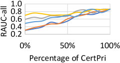
(a) +AdapS (ID: 22)

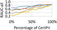
(b) +AdapC (ID: 23)

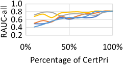
(c) +AdapM (ID: 24)

Figure 4: The promotion results of CertPri for baselines through combining it with each baseline.

Prioritization robustness. In all cases, CertPri always performs the most robust prioritization results against various adaptive attacks, which facilitates stable identification of bug-revealing inputs. For instance, in Table XI, the average RobR values of CertPri against adaptive attacks range from 99.93% to 103.60%, which is 1.50$\sim$1.71 times that of baselines. The outstanding performance of CertPri is mainly because it simplifies the prioritization task into a lower bound measure of the movement cost, which has been formally guaranteed in Section III-B.

Utility of robustness. CertPri is not only immune to various adaptive attacks, but also facilitates the robustness of baselines through weighted combinations. For instance, in Figure 4, all curves show an upward trend after combining with CertPri and are always higher than their initial value without CertPri. Furthermore, we speculate that for an empirical prioritization method that outperforms CertPri in general, it can be combined with CertPri to improve robustness against adaptive attacks.

Answer to RQ3: CertPri largely outperforms baselines in terms of robust prioritization with average robustness improvements of 41.37%$\sim$98.91%. Besides, its robustness can be leveraged to facilitate other methods.

V-D Generalizability (RQ4)

How generic is CertPri in prioritizing test inputs?

When reporting the generalizability, we focus on the ranking of RAUC values for different methods in each subject. The evaluation results are illustrated as radar charts in Figure 5.

Implementation details for generalizability evaluation. (1) Calculate the GenRew value of each dimension separately. Take the task dimension as an example, which includes classification and regression. First, we select all subjects belonging to the classification task and calculate GenRew according to Equation (9), denoted as GR_c. Then, we select all subjects belonging to the regression task and compute GenRew, denoted as GR_r. Finally, we compute the average of GR_c and GR_r as the task-dimensional GenRew. (2) Repeat the above operations for the remaining 5 dimensions (i.e., data form/type, structure, training/prioritization scenarios).

Prioritization generalizability. CertPri always outperforms all baselines against various dimensions in terms of all average GenRew values. For instance, in Figure 5, the area of CertPri covers all baselines. More specifically, the average GenRew values of CertPri range from 0.9040 to 0.9813 with average improvements of 32.81%$\sim$238.54% compared with baselines. This is mainly because CertPri’s calculation only involves gradient derivation based on back propagation, which is easy to implement for any DNN. Thus, CertPri can be generalized to various dimensions.

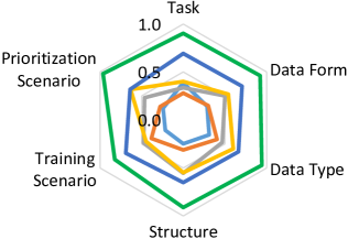
(a) GenRew of RAUC-300

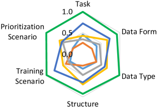
(b) GenRew of RAUC-all

Figure 5: Generalizability comparison for six dimensions across all subjects, measured by GenRew.

Answer to RQ4: CertPri is more generic than baselines in all six dimensions with average generalizability improvements of 32.81%$\sim$238.54%.

V-E Guidance (RQ5)

Can CertPri guide the retraining of DNNs to improve their performance and robustness?

When reporting the guidance, we focus on two aspects: accuracy improvement and robustness improvement for DNNs. The evaluation results are illustrated as boxplots in Figure 6.

Implementation details for guidance evaluation. Take the classification on CIFAR10 as an example. (1) In terms of performance (ID: 1, 9), we sample original data prioritized at the front 1% and 5% in the training set. We set epoch=5 for retraining due to the small number of data. We compare the test accuracy. (2) In terms of robustness (ID: 3-5, 11-13), we sample adversarial data prioritized at the front 1% and 5% in the adversarial set. We mix the sampled data with the original training set, and set epoch=2 for retraining due to a large number of data. Repeat the above operations 5 times.

Accuracy improvement for DNNs. The original test inputs prioritized at the front facilitate model accuracy through retraining, where CertPri demonstrates SOTA accuracy improvement. For instance, in Figure 6 (a), the box position of CertPri is significantly higher than that of baselines. More specifically, the average accuracy improvements of CertPri range from 4.50% to 8.36%, which is 1.65$\sim$3.47 times that of baselines. It demonstrates CertPri’s outstanding guidance for the accuracy improvement of DNNs.

Robustness improvement for DNNs. The adversarial test inputs prioritized at the front facilitate model robustness through retraining, where CertPri outperforms surprise-based methods and shows competitive performance with confidence-based and mutation-based methods. For instance, in Figure 6 (b), the box position of CertPri is significantly higher than that of LSA and DSA, while close to that of MCP, DeepGini and PRIMA. It demonstrates CertPri’s guidance for the robustness improvement of DNNs.

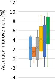
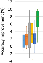
(a) Accuracy improvement

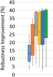
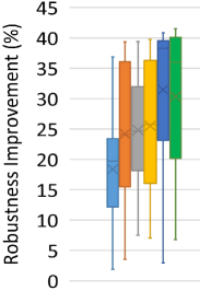
(b) Robustness improvement

Figure 6: Guidance comparison of accuracy and robustness improvements for different methods under the first 1% and 5% prioritized data sampling (from left to right).

Answer to RQ5: CertPri guides DNNs’ retraining with only first 1% or 5% prioritized test inputs, which improves accuracy by 6.15% and robustness by 31.07% on average.

VI Threats to Validity

Three aspects may become the threats to validity of CertPri.

The internal threat to validity mainly lies in the center position determination. There are differences in movement costs to reach different centers, especially for non-uniformly distributed data in feature space. To reduce the internal threat, we customize the center position for each test input in Definition 1, i.e., relative center. Besides, we collect a large number of subjects with great diversity, and perform extensive experiments to verify CertPri’s utility.

The external threats to validity mainly lie in the non-differentiable component and gradient vanishing. To reduce these threats, we further extend Theorems 1 and 2 to a special case of non-differentiable functions, i.e., a model with ReLU activation, as shown in https://anonymous.4open.science/r/CertPri/SupplementaryMaterials.pdf. Then, we leverage batch normalization and non-saturating activation to reduce the probability of gradient vanishing and enlarge the sampling radius of the hyper-ball.

The construct threats to validity mainly lie in the hyperparameters in CertPri, including $N_{b}$, $N_{rsb}$ and $\mathcal{R}$ values in Algorithms 1. Larger hyperparameter values produce better effectiveness, but reduce efficiency. To reduce the threat from the hyperparameters, we conduct a double-minimum strategy. Besides, the norm value $p$=2 and the extreme value distribution type is Weibull in our experiments. In future work, we can explore prioritization results for various norm types and extreme value distributions.

VII Related Works

To solve the labeling-cost problem in DNN testing, several works on test input prioritization are proposed [23, 24, 28, 25, 22, 29, 27, 68, 24, 69].

From the perspective of statistical analysis, there are coverage-based [20, 12, 26, 70], surprise-based [27, 22, 28, 68], and confidence-based methods [23, 25, 29]. Feng et al. [23] comprehensively analyzed coverage-based methods and concluded that their effectiveness and efficiency are unsatisfactory for prioritization tasks. To improve effectiveness, Byun et al. [22] prioritized test inputs based on surprise adequacy metrics. Zhang et al. [27] observed the activation pattern of neurons, and produced prioritization results according to the activation patterns between the training set and test inputs. Ma et al. [68] considered the interaction between test inputs and model uncertainty, and determined bug-revealing inputs with higher uncertainty. These surprise-based methods improve performance, but their prioritization results are related to the training set quality. Furthermore, Zhang et al. [29] prioritized test inputs based on noise sensitivity analysis, independent of the training set. Shen et al. [25] proposed MCP, in which clusters test inputs into the boundary areas and specify the priority to select them evenly. Feng et al. [23] proposed DeepGini, which prioritizes test input by measuring set impurity. These confidence-based methods are effective and efficient, but only for classification tasks.

Drawing lessons from the mutation view in software engineering [71, 72], Wang et al. [24] proposed PRIMA, which gives priority to test inputs that generate different predictions through diversity mutations (i.e., input-level and model-level). PRIMA demonstrates SOTA performance, but cannot be applied to black-box scenarios.

Different from them, CertPri prioritizes test inputs based on movement view in feature space. Besides, it takes robustness certification into account. Robustness certification [48, 45, 73] provides formal guarantees for DNNs against norm bounded attacks, which also facilitates CertPri against adaptive attacks. To the best of our knowledge, CertPri is the first to consider the prioritization robustness and introduce formal guarantees to provide certifiability.

VIII Conclusions

We propose a certifiable prioritization method for bug-revealing test input identification earlier, CertPri, to efficiently solve the labeling-cost problem in DNN testing and build trustworthy deep learning systems. CertPri provides a new perspective on prioritization, which reduces the problem of measuring misbehavior probability to the problem of measuring the movement difficulty in feature space. Based on this view, we give formal guarantees about lower bounds $\gamma_{L}$ on movement cost, and compute $\gamma_{L}$ value based on GEVT. The priority of each test input is determined in ascending order of $\gamma_{L}$ value. Furthermore, we generalize CertPri in black-box scenarios by gradient estimation. CertPri is compared with baseline on various tasks, data forms, data types, model structures, training and prioritization scenarios. The results show that CertPri outperforms baselines in terms of effectiveness, efficiency, robustness, generalizability and guidance.

References

- [1] Y. LeCun, Y. Bengio, and G. Hinton, “Deep learning,” Nature, vol. 521, no. 7553, pp. 436–444, 2015.
- [2] K. Simonyan and A. Zisserman, “Very deep convolutional networks for large-scale image recognition,” in 3rd International Conference on Learning Representations. San Diego, CA, USA: OpenReview.net, 2014, pp. 1–14.
- [3] K. He, X. Zhang, S. Ren, and J. Sun, “Deep residual learning for image recognition,” in IEEE Conference on Computer Vision and Pattern Recognition. Las Vegas, NV, USA: Computer Vision Foundation / IEEE Computer Society, 2016, pp. 770–778.
- [4] A. Krizhevsky, I. Sutskever, and G. E. Hinton, “Imagenet classification with deep convolutional neural networks,” Commun. ACM, vol. 60, no. 6, pp. 84–90, 2017.
- [5] B. Alshemali and J. Kalita, “Improving the reliability of deep neural networks in nlp: A review,” Knowledge-Based Systems, vol. 191, no. 1, pp. 1–19, 2020.
- [6] K. Shuang, Y. Tan, Z. Cai, and Y. Sun, “Natural language modeling with syntactic structure dependency,” Information Sciences, vol. 523, no. 1, pp. 220–233, 2020.
- [7] H. Zhang, W. K. Chan, and Ieee, “Apricot: A weight-adaptation approach to fixing deep learning models,” in 34th IEEE/ACM International Conference on Automated Software Engineering. San Diego, CA, USA: IEEE, 2019, pp. 376–387.
- [8] J. Chen, K. Hu, Y. Yu, Z. Chen, Q. Xuan, Y. Liu, and V. Filkov, “Software visualization and deep transfer learning for effective software defect prediction,” in 42nd International Conference on Software Engineering. Seoul, South Korea: ACM, 2020, pp. 578–589.
- [9] Y. Tian, K. Pei, S. Jana, and B. Ray, “Deeptest: Automated testing of deep neural network driven autonomous cars,” in 40th ACM/IEEE International Conference on Software Engineering. Gothenburg, Sweden: ACM, 2018, pp. 303–314.
- [10] H. F. Eniser, S. Gerasimou, and A. Sen, “Deepfault: Fault localization for deep neural networks,” in Fundamental Approaches to Software Engineering-22nd International Conference. Prague, Czech Republic: Springer, 2019, pp. 171–191.
- [11] Q. Hu, L. Ma, X. Xie, B. Yu, Y. Liu, and J. Zhao, “Deepmutation++: a mutation testing framework for deep learning systems,” in 34th IEEE/ACM International Conference on Automated Software Engineering. San Diego, CA, USA: IEEE, 2019, pp. 1158–1161.
- [12] K. Pei, Y. Cao, J. Yang, and S. Jana, “Deepxplore: automated whitebox testing of deep learning systems,” Commun. ACM, vol. 62, no. 11, pp. 137–145, 2019.
- [13] C. Ziegler, “A google self-driving car caused a crash for the first time,” The Verge, 2016. [Online]. Available: https://www.theverge.com/2016/2/29/11134344/google-self-driving-car-crash-report
- [14] J. Stewart, “Tesla’s autopilot was involved in another deadly car crash,” Wired, 2018. [Online]. Available: https://www.wired.com/story/tesla-autopilot-self-driving-crash-california/
- [15] L. Alex, “Uber is giving up on self-driving cars in california after deadly crash,” Vice Media Group, 2018. [Online]. Available: https://www.vice.com/en/article/9kga85/uber-is-giving-up-on-self-driving-cars-in-california-after-deadly-crash
- [16] H. Zheng, Z. Chen, T. Du, X. Zhang, Y. Cheng, S. Ji, J. Wang, Y. Yu, and J. Chen, “Neuronfair: Interpretable white-box fairness testing through biased neuron identification,” in 44th International Conference on Software Engineering. New York, NY, USA: ACM, 2022, pp. 1–13.
- [17] F. Harel-Canada, L. Wang, M. A. Gulzar, Q. Gu, and M. Kim, “Is neuron coverage a meaningful measure for testing deep neural networks?” in ACM Joint Meeting on European Software Engineering Conference and Symposium on the Foundations of Software Engineering. Virtual Event, USA: ACM, 2020, pp. 851–862.
- [18] X. Xie, L. Ma, F. Juefei-Xu, M. Xue, H. Chen, Y. Liu, J. Zhao, B. Li, J. Yin, and S. See, “Deephunter: A coverage-guided fuzz testing framework for deep neural networks,” in 28th ACM SIGSOFT International Symposium on Software Testing and Analysis. Beijing, China: ACM, 2019, pp. 146–157.
- [19] J. Guo, Y. Jiang, Y. Zhao, Q. Chen, and J. Sun, “Dlfuzz: Differential fuzzing testing of deep learning systems,” in ACM Joint Meeting on European Software Engineering Conference and Symposium on the Foundations of Software Engineering. Lake Buena Vista, FL, USA: ACM, 2018, pp. 739–743.
- [20] L. Ma, F. Juefei-Xu, F. Zhang, J. Sun, M. Xue, B. Li, C. Chen, T. Su, L. Li, and Y. Liu, “Deepgauge: Multi-granularity testing criteria for deep learning systems,” in 33rd ACM/IEEE International Conference on Automated Software Engineering. Montpellier, France: ACM, 2018, pp. 120–131.
- [21] J. Chen, Z. Wu, Z. Wang, H. You, L. Zhang, and M. Yan, “Practical accuracy estimation for efficient deep neural network testing,” ACM Transactions on Software Engineering and Methodology, vol. 29, no. 4, pp. 1–35, 2020.
- [22] T. Byun, V. Sharma, A. Vijayakumar, S. Rayadurgam, and D. D. Cofer, “Input prioritization for testing neural networks,” in IEEE International Conference On Artificial Intelligence Testing, AITest 2019. Newark, CA, USA: IEEE, 2019, pp. 63–70.
- [23] Y. Feng, Q. Shi, X. Gao, J. Wan, C. Fang, and Z. Chen, “Deepgini: prioritizing massive tests to enhance the robustness of deep neural networks,” in 29th ACM SIGSOFT International Symposium on Software Testing and Analysis. Virtual Event, USA: ACM, 2020, pp. 177–188.
- [24] Z. Wang, H. You, J. Chen, Y. Zhang, X. Dong, and W. Zhang, “Prioritizing test inputs for deep neural networks via mutation analysis,” in 43rd IEEE/ACM International Conference on Software Engineering. Madrid, Spain: IEEE, 2021, pp. 397–409.
- [25] W. Shen, Y. Li, L. Chen, Y. Han, Y. Zhou, and B. Xu, “Multiple-boundary clustering and prioritization to promote neural network retraining,” in 35th IEEE/ACM International Conference on Automated Software Engineering. Melbourne, Australia: IEEE, 2020, pp. 410–422.
- [26] M. Wicker, X. Huang, and M. Kwiatkowska, “Feature-guided black-box safety testing of deep neural networks,” in Tools and Algorithms for the Construction and Analysis of Systems - 24th International Conference, TACAS 2018, vol. 10805. Thessaloniki, Greece: Springer, 2018, pp. 408–426.
- [27] K. Zhang, Y. Zhang, L. Zhang, H. Gao, R. Yan, and J. Yan, “Neuron activation frequency based test case prioritization,” in International Symposium on Theoretical Aspects of Software Engineering. Hangzhou, China: IEEE, 2020, pp. 81–88.
- [28] J. Kim, R. Feldt, and S. Yoo, “Guiding deep learning system testing using surprise adequacy,” in 41st IEEE/ACM International Conference on Software Engineering. Montreal, QC, Canada: IEEE / ACM, 2019, pp. 1039–1049.
- [29] L. Zhang, X. Sun, Y. Li, and Z. Zhang, “A noise-sensitivity-analysis-based test prioritization technique for deep neural networks,” CoRR, vol. abs/1901.00054, pp. 1–8, 2019. [Online]. Available: http://arxiv.org/abs/1901.00054
- [30] I. J. Goodfellow, J. Shlens, and C. Szegedy, “Explaining and harnessing adversarial examples,” in 3rd International Conference on Learning Representations. San Diego, CA, USA: OpenReview.net, 2014, pp. 1–11.
- [31] Y. Dong, F. Liao, T. Pang, H. Su, J. Zhu, X. Hu, and J. Li, “Boosting adversarial attacks with momentum,” in IEEE Conference on Computer Vision and Pattern Recognition. Salt Lake City, UT, USA: Computer Vision Foundation / IEEE Computer Society, 2018, pp. 9185–9193.
- [32] J. Chen, H. Zheng, H. Xiong, S. Shen, and M. Su, “Mag-gan: Massive attack generator via gan,” Information Sciences, vol. 536, no. 1, pp. 67–90, 2020.
- [33] S.-M. Moosavi-Dezfooli, A. Fawzi, and P. Frossard, “Deepfool: a simple and accurate method to fool deep neural networks,” in IEEE Conference on Computer Vision and Pattern Recognition. Las Vegas, NV, USA: IEEE Computer Society, 2016, pp. 2574–2582.
- [34] C. Shorten and T. M. Khoshgoftaar, “A survey on image data augmentation for deep learning,” Journal of Big Data, vol. 6, no. 1, pp. 1–48, 2019.
- [35] B. Sun, N.-H. Tsai, F. Liu, R. Yu, and H. Su, “Adversarial defense by stratified convolutional sparse coding,” in IEEE Conference on Computer Vision and Pattern Recognition. Long Beach, CA, USA: Computer Vision Foundation / IEEE, 2019, pp. 11 447–11 456.
- [36] A. Mustafa, S. Khan, M. Hayat, R. Goecke, J. Shen, and L. Shao, “Adversarial defense by restricting the hidden space of deep neural networks,” in IEEE International Conference on Computer Vision. Seoul, South Korea: IEEE, 2019, pp. 3384–3393.
- [37] A. S. Rakin, H. Zhezhi, and F. Deliang, “Parametric noise injection: trainable randomness to improve deep neural network robustness against adversarial attack,” in IEEE Conference on Computer Vision and Pattern Recognition. Long Beach, CA, USA: Computer Vision Foundation / IEEE, 2019, pp. 588–597.
- [38] Y. Li, J. Hua, H. Wang, C. Chen, and Y. Liu, “Deeppayload: Black-box backdoor attack on deep learning models through neural payload injection,” in 43rd IEEE/ACM International Conference on Software Engineering (ICSE 2021). Madrid, Spain: IEEE, 2021, pp. 263–274.
- [39] R. K. E. Bellamy, K. Dey, M. Hind, S. C. Hoffman, S. Houde, K. Kannan, P. Lohia, J. Martino, S. Mehta, A. Mojsilovic, S. Nagar, K. N. Ramamurthy, J. T. Richards, D. Saha, P. Sattigeri, M. Singh, K. R. Varshney, and Y. Zhang, “AI fairness 360: An extensible toolkit for detecting and mitigating algorithmic bias,” IBM J. Res. Dev., vol. 63, no. 4/5, pp. 1–15, 2019. [Online]. Available: https://doi.org/10.1147/JRD.2019.2942287
- [40] Z. Zhang, P. Cui, and W. Zhu, “Deep learning on graphs: A survey,” IEEE Transactions on Knowledge and Data Engineering, vol. 34, no. 1, pp. 249–270, 2020.
- [41] H. Zheng, J. Chen, H. Du, W. Zhu, S. Ji, and X. Zhang, “Grip-gan: An attack-free defense through general robust inverse perturbation,” IEEE Transactions on Dependable and Secure Computing, pp. 1–18, 2021.
- [42] O. Russakovsky, J. Deng, H. Su, J. Krause, S. Satheesh, S. Ma, Z. Huang, A. Karpathy, A. Khosla, M. Bernstein, A. C. Berg, and L. Fei-Fei, “ImageNet Large Scale Visual Recognition Challenge,” International Journal of Computer Vision (IJCV), vol. 115, no. 3, pp. 211–252, 2015.
- [43] R. Paulavičius and J. Žilinskas, “Analysis of different norms and corresponding lipschitz constants for global optimization,” Technological and Economic Development of Economy, vol. 12, no. 4, pp. 301–306, 2006.
- [44] B. Gnedenko, “Sur la distribution limite du terme maximum d’une serie aleatoire,” Annals of Mathematics, vol. 44, no. 3, pp. 423–453, 1943.
- [45] T. Weng, H. Zhang, P. Chen, J. Yi, D. Su, Y. Gao, C. Hsieh, and L. Daniel, “Evaluating the robustness of neural networks: An extreme value theory approach,” in 6th International Conference on Learning Representations (ICLR 2018). Vancouver, BC, Canada: OpenReview.net, 2018, pp. 1–18.
- [46] A. Tampuu, T. Matiisen, M. Semikin, D. Fishman, and N. Muhammad, “A survey of end-to-end driving: Architectures and training methods,” IEEE Transactions on Neural Networks and Learning Systems, vol. 33, no. 4, pp. 1364–1384, 2022.
- [47] P. Chen, H. Zhang, Y. Sharma, J. Yi, and C. Hsieh, “ZOO: zeroth order optimization based black-box attacks to deep neural networks without training substitute models,” in Proceedings of the 10th ACM Workshop on Artificial Intelligence and Security, AISec@CCS 2017. Dallas, TX, USA: ACM, 2017, pp. 15–26.
- [48] T. Du, S. Ji, L. Shen, Y. Zhang, J. Li, J. Shi, C. Fang, J. Yin, R. Beyah, and T. Wang, “Cert-rnn: Towards certifying the robustness of recurrent neural networks,” in Conference on Computer and Communications Security (CCS 2021). Virtual Event, Republic of Korea: ACM, 2021, pp. 516–534.
- [49] J. S. Denker and Y. LeCun, “Transforming neural-net output levels to probability distributions,” in Advances in Neural Information Processing Systems 3 (NIPS 1990). Denver, Colorado, USA: Morgan Kaufmann, 1990, pp. 853–859.
- [50] K. Eckle and J. Schmidt-Hieber, “A comparison of deep networks with relu activation function and linear spline-type methods,” Neural Networks, vol. 110, pp. 232–242, 2019.
- [51] J. Chen, H. Zheng, W. Shangguan, L. Liu, and S. Ji, “Act-detector: Adaptive channel transformation-based light-weighted detector for adversarial attacks,” Information Sciences, vol. 564, pp. 163–192, 2021.
- [52] Y. LeCun, B. Boser, J. S. Denker, D. Henderson, R. E. Howard, W. Hubbard, and L. D. Jackel, “Backpropagation applied to handwritten zip code recognition,” Neural Computation, vol. 1, no. 4, pp. 541–551, 1989.
- [53] L. Van der Maaten and G. Hinton, “Visualizing data using t-sne,” Journal of machine learning research, vol. 9, no. 11, pp. 2579–2605, 2008.
- [54] S.-i. Amari, “Backpropagation and stochastic gradient descent method,” Neurocomputing, vol. 5, no. 4, pp. 185–196, 1993.
- [55] A. Krizhevsky, “Learning multiple layers of features from tiny images,” Computer Science Department, University of Toronto, Tech. Rep., 2009.
- [56] Y. Deng, J. X. Zheng, T. Zhang, C. Chen, G. Lou, and M. Kim, “An analysis of adversarial attacks and defenses on autonomous driving models,” in IEEE International Conference on Pervasive Computing and Communications (PerCom 2020). Austin, TX, USA: IEEE, 2020, pp. 1–10.
- [57] H. Xiao, K. Rasul, and R. Vollgraf, “Fashion-mnist: a novel image dataset for benchmarking machine learning algorithms,” ArXiv Preprint, vol. abs/1708.07747, pp. 1–6, 2017. [Online]. Available: https://arxiv.org/abs/1708.07747
- [58] A. L. Maas, R. E. Daly, P. T. Pham, D. Huang, A. Y. Ng, and C. Potts, “Learning word vectors for sentiment analysis,” in The 49th Annual Meeting of the Association for Computational Linguistics: Human Language Technologies. Portland, Oregon, USA: Association for Computational Linguistics, 2011, pp. 142–150.
- [59] T. J. O’Shea and N. West, “Radio machine learning dataset generation with gnu radio,” in Proceedings of the GNU Radio Conference, 2016, pp. 1–10.
- [60] A. McCallum, K. Nigam, J. Rennie, and K. Seymore, “Automating the construction of internet portals with machine learning,” Inf. Retr., vol. 3, no. 2, pp. 127–163, 2000.
- [61] R. Kohavi, “Scaling up the accuracy of naive-bayes classifiers: A decision-tree hybrid,” in Proceedings of the Second International Conference on Knowledge Discovery and Data Mining (KDD-96), Portland, Oregon, USA. Menlo Park, CA: AAAI Press, 1996, pp. 202–207. [Online]. Available: http://www.aaai.org/Library/KDD/1996/kdd96-033.php
- [62] A. Kurakin, I. J. Goodfellow, and S. Bengio, “Adversarial examples in the physical world,” in 5th International Conference on Learning Representations (ICLR 2017). Toulon, France: OpenReview.net, 2017, pp. 1–14.
- [63] N. Carlini and D. Wagner, “Towards evaluating the robustness of neural networks,” in IEEE Symposium on Security and Privacy (SP 2017). San Jose, CA, USA: IEEE Computer Society, 2017, pp. 39–57.
- [64] J. Chen, H. Zheng, H. Xiong, R. Chen, T. Du, Z. Hong, and S. Ji, “Finefool: A novel DNN object contour attack on image recognition based on the attention perturbation adversarial technique,” Comput. Secur., vol. 104, p. 102220, 2021.
- [65] H. Hosseini and R. Poovendran, “Semantic adversarial examples,” in IEEE Conference on Computer Vision and Pattern Recognition Workshops, (CVPR Workshops 2018). Salt Lake City, UT, USA: Computer Vision Foundation / IEEE Computer Society, 2018, pp. 1614–1619.
- [66] J. Chen, L. Zhang, H. Zheng, X. Wang, and Z. Ming, “Deeppoison: Feature transfer based stealthy poisoning attack for dnns,” IEEE Trans. Circuits Syst. II Express Briefs, vol. 68, no. 7, pp. 2618–2622, 2021.
- [67] S. Ioffe and C. Szegedy, “Batch normalization: Accelerating deep network training by reducing internal covariate shift,” in Proceedings of the 32nd International Conference on Machine Learning (ICML 2015), vol. 37. Lille, France: JMLR.org, 2015, pp. 448–456.
- [68] W. Ma, M. Papadakis, A. Tsakmalis, M. Cordy, and Y. L. Traon, “Test selection for deep learning systems,” ACM Transactions on Software Engineering and Methodology (TOSEM), vol. 30, no. 2, pp. 1–22, 2021.
- [69] X. Xie, P. Yin, and S. Chen, “Boosting the revealing of detected violations in deep learning testing: A diversity-guided method,” in 37th IEEE/ACM International Conference on Automated Software Engineering, ASE 2022, Rochester, MI, USA, October 10-14, 2022. ACM, 2022, pp. 17:1–17:13.
- [70] X. Xie, T. Li, J. Wang, L. Ma, Q. Guo, F. Juefei-Xu, and Y. Liu, “NPC: neuron path coverage via characterizing decision logic of deep neural networks,” ACM Trans. Softw. Eng. Methodol., vol. 31, no. 3, pp. 47:1–47:27, 2022.
- [71] Y. Lou, D. Hao, and L. Zhang, “Mutation-based test-case prioritization in software evolution,” in 2015 IEEE 26th International Symposium on Software Reliability Engineering (ISSRE). Gaithersbury, MD, USA: IEEE Computer Society, 2015, pp. 46–57.
- [72] D. Shin, S. Yoo, M. Papadakis, and D.-H. Bae, “Empirical evaluation of mutation-based test case prioritization techniques,” Software Testing, Verification and Reliability, vol. 29, no. 1-2, pp. 1–2, 2019.
- [73] C. Ko, Z. Lyu, L. Weng, L. Daniel, N. Wong, and D. Lin, “POPQORN: quantifying robustness of recurrent neural networks,” in Proceedings of the 36th International Conference on Machine Learning, ICML 2019, ser. Proceedings of Machine Learning Research, vol. 97. Long Beach, California, USA: PMLR, 2019, pp. 3468–3477.