Sparse Gaussian Graphical Models with Discrete Optimization: Computational and Statistical Perspectives

Abstract

We consider the problem of learning a sparse graph underlying an undirected Gaussian graphical model, a key problem in statistical machine learning. Given $n$ samples from a multivariate Gaussian distribution with $p$ variables, the goal is to estimate the $p\times p$ inverse covariance matrix (aka precision matrix), assuming it is sparse (i.e., has a few nonzero entries). We propose GraphL0BnB, a new estimator based on an $\ell_{0}$-penalized version of the pseudolikelihood function, while most earlier approaches are based on the $\ell_{1}$-relaxation. Our estimator can be formulated as a convex mixed integer program (MIP) which can be difficult to compute at scale using off-the-shelf commercial solvers. To solve the MIP, we propose a custom nonlinear branch-and-bound (BnB) framework that solves node relaxations with tailored first-order methods. As a by-product of our BnB framework, we propose large-scale solvers for obtaining good primal solutions that are of independent interest. We derive novel statistical guarantees (estimation and variable selection) for our estimator and discuss how our approach improves upon existing estimators. Our numerical experiments on real/synthetic datasets suggest that our method can solve, to near-optimality, problem instances with $p=10^{4}$ — corresponding to a symmetric matrix of size $p\times p$ with $p^{2}/2$ binary variables. We demonstrate the usefulness of GraphL0BnB versus various state-of-the-art approaches on a range of datasets.

1 Introduction

Gaussian Graphical Models (GGM), due to Dempster (1972), are amongst the most widely used tools in multivariate statistics and machine learning (Hastie et al. (2009, Chapter 17) and Wainwright (2019, Chapter 11)). Formally, in a GGM, we are given $n$ samples $\bm{x}^{(1)},\cdots,\bm{x}^{(n)}\in\mathbb{R}^{p}$ from a multivariate normal distribution ${\mathcal{N}}(\bm{0},\bm{\Sigma}^{*})$ where $\bm{\Sigma}^{*}$ is an unknown $p\times p$ positive definite matrix. Our goal is to estimate the inverse of the covariance matrix $\bm{\Sigma}^{*}$, known as the precision matrix and denoted as $\bm{\Theta}^{*}$. Obtaining a sparse estimate of $\bm{\Theta}^{*}$ (i.e., one with only a few nonzero coordinates) is an important methodological problem with an array of applications (Hastie et al. 2009, Wainwright 2019), and has garnered significant attention in statistical learning. Particularly, a zero entry in $\bm{\Theta}^{*}$ indicates conditional independence: For a pair $(i,j)$, having $\theta^{*}_{ij}=0$ implies features $i,j$ are independent when conditioning on the other variables. Our goal is to estimate a sparse precision matrix $\hat{\bm{\Theta}}$ (say), such that it is close to the true precision matrix $\bm{\Theta}^{*}$ in a suitable metric, as discussed below.

The topic of sparse GGMs is quite vast—we first present an overview of some well-known algorithms and then summarize our key contributions in this paper.

1.1 Background and Literature Review

Numerous algorithms have been proposed for sparse GGMs. Generally, these methods aim to minimize a regularized loss function, where the regularization term encourages sparsity in the precision matrix estimate. A popular approach involves the minimization of an $\ell_{1}$-regularized negative log-likelihood function, known as Graphical Lasso (Friedman et al. 2008). Graphical Lasso given by a convex semidefinite program enjoys good statistical and computational properties (Ravikumar et al. 2008, Mazumder and Hastie 2012). CLIME (Cai et al. 2011) is another approach with strong theoretical underpinnings: it is based on constrained $\ell_{1}$-norm minimization and is given by a linear program. Another well-known approach is the node-wise $\ell_{1}$-regularized regression framework of Meinshausen and Bühlmann (2006), which involves solving $p$ separate Lasso regression problems.

The current paper focuses on a pseudo-likelihood based approach for sparse GGMs. The pseudo-likelihood approach with origins in spatial analysis (Besag 1975) approximates the Gaussian likelihood by the product of conditional likelihood functions of each variable, given the rest. In an early work Peng et al. (2009) explored pseudo-likelihood with $\ell_{1}$ regularization in the context of sparse GGMs. They show their method performs well numerically and present an asymptotic analysis of their algorithm when $n,p\to\infty$. Symmetric Lasso (Friedman et al. 2010b) and CONCORD (Khare et al. 2015) are other algorithms based on pseudo-likelihood with strong empirical performance.

A fairly recent and less explored approach to GGMs is based on discrete optimization. Since the work of Bertsimas et al. (2016) on subset selection in linear regression, there has been considerable interest in exploring statistical problems with a combinatorial structure using tools from Mixed Integer Programming (MIP) (Wolsey and Nemhauser 1999) and relatives. Specialized algorithms have been recently explored to address MIP-based statistical problems in sparse linear regression (Bertsimas and Parys 2020, Hazimeh et al. 2022, Hazimeh and Mazumder 2020, Mazumder et al. 2023), sparse principal component analysis (Dey et al. 2022, Behdin and Mazumder 2021, see also references therein), among others. In contrast, the literature on using MIP approaches for sparse GGMs, remains relatively less explored. Bertsimas et al. (2020) consider a MIP approach for $\ell_{0}$-constrained maximum likelihood GGM estimation—their specialized algorithm can address problems with $p\approx 100$. Another approach is the node-wise procedure of Misra et al. (2020), which requires solving $p$-many $\ell_{0}$ regularized linear regression problems. Recently, Fattahi and Gómez (2021) explore $\ell_{0}$ regularization for sparse GGMs in the context of time-series problems.

We mention some existing results on statistical properties of sparse precision matrix estimation. Let $k$ denote an upper bound on the number of nonzero coordinates in each row/column of $\bm{\Theta}^{*}$. To have a consistent estimate of $\bm{\Theta}^{*}$ (in terms of the Frobenius norm of the estimation error) we need $n\gtrsim kp\log p$ samples (Rothman et al. 2008). This implies that consistent estimation is only possible when $kp/n\to 0$, which corresponds to the low-dimensional setting. In the high-dimensional setting where $p\gg n$, one is often interested in estimating the true support of $\bm{\Theta}^{*}$ with high probability. Under certain non-degeneracy conditions, $n\gtrsim k\log p$ samples are required for a consistent estimation of the support of $\bm{\Theta}^{*}$ (Wang et al. 2010). This suggests that support recovery is possible even when $p/n\to\infty$.

1.2 Outline of our Approach and Contributions

We propose a new $\ell_{0}$-regularized pseudo-likelihood-based estimator, GraphL0BnB, with good statistical guarantees and computational performance. Our estimator is based on a MIP: it can be written as minimizing a convex objective function over a mixed integer second-order cone. As a result, commercial solvers such as Mosek can be used to solve the problem for small-scale instances $p\leq 100$. We propose specialized exact (and approximate) algorithms for improved computational scalability for our estimator. In addition to computation, we study the statistical properties of the estimator as outlined below.

Optimization Algorithms: We propose and implement (i) approximate methods, to obtain high-quality feasible solutions quickly (ii) globally optimal methods based on a specialized nonlinear Branch-and-Bound (BnB) solver. Our standalone BnB solver does not rely on commercial MIP solvers. It can solve, with optimality certificates, problem instances with $p\approx 10,000$ (with $50\times 10^{6}$ binary variables) when the optimal solution is sufficiently sparse in less than an hour. Our approximate algorithms are generally faster than the exact methods and can play an important role in the latter (e.g, by providing good feasible solutions). We note that the objective function that we are dealing with involves logarithmic and quadratic-over-linear terms (see Section 2). This requires proposing new algorithms for solving node relaxation and obtaining incumbents. We also establish novel convergence guarantees for our algorithms that extend existing results. Our node relaxation solver uses cyclic coordinate descent (Tseng 2001) along with active set updates for computational efficiency. We discuss methods to efficiently generate dual bounds, which are important for our BnB method. Our approximate methods extend the work of Hazimeh and Mazumder (2020), and our BnB framework is inspired by the work of Hazimeh et al. (2022) both proposed for sparse linear regression. We note that the specific structure of our objective function and the problem scale present technical difficulties making our GGM approach different from earlier work.

Statistical Properties: We study both the estimation and variable selection properties of our proposed estimator. We show that our estimator has an estimation error (Frobenius norm) bound scaling as $\sqrt{kp\log p/n}$, where $k$ is an upper bound on the total number of nonzero coordinates in each row/column of $\bm{\Theta}^{*}$. In terms of variable selection, we show that under certain regularity conditions, if $n\gtrsim k\log p$, our estimator is able to recover the support of $\bm{\Theta}^{*}$ correctly with high probability. The non-degeneracy condition needed for consistent variable selection for our method is milder than the earlier ones. This is due to certain symmetry structures we enforce on the precision matrix as a part of our estimation criterion. Our non-asymptotic estimation error bounds and support recovery guarantees are a novel contribution in the context of pseudo-likelihood-based sparse GGMs. Moreover, due to the specific structures of our problem, most earlier proof techniques developed do not apply to our estimator directly, and we develop new techniques for our analysis.

Numerical Results: We compare our approach with other existing methods in terms of both statistical performance and computational efficiency on both synthetic and real datasets. Our numerical results indicate that our optimization framework can solve instances with $p\approx 10,000$ in less than an hour, while earlier pseudo-likelihood-based estimators appear to be limited to instances with $p\leq 3000$ or so. Moreover, we observe that GraphL0BnB enjoys better statistical performance (estimation and variable selection) on synthetic and real datasets compared to popularly used $\ell_{1}$-based methods such as CLIME and Graphical Lasso.

Our contributions in this paper can be summarized as follows:

1. We propose an $\ell_{0}$-regularized pseudo-likelihood estimator GraphL0BnB for sparse GGMs. Our MIP-based estimator can be formulated as minimizing a convex objective with mixed integer second order conic constraints.

2. We propose a custom branch-and-bound (BnB) method for the MIP. Our open-source BnB solver can solve (with optimality certificates) certain problem-instances with $p\approx 10,000$ (involving $p\times p$ precision matrices) in less than an hour. As a by-product of our framework, we also propose new approximate algorithms that can be much faster than the optimal methods.

3. We derive novel statistical (both estimation and variable selection) guarantees for our estimator and discuss how they can improve upon existing estimators.

4. Numerical experiments on real and synthetic datasets show the promise of GraphL0BnB over popular alternatives for sparse GGMs in terms of both runtime and statistical performance.

Organization of paper

In Section 2, we introduce GraphL0BnB. In Section 3, we provide a computational framework for our proposed estimator. In Section 4, we analyze the statistical properties of our proposed estimator. Section 5 presents numerical experiments on both synthetic and real datasets. The derivations and proofs in the computational and statistical parts are deferred to Appendices A and B.

Notations.

For the data matrix $\bm{X}\in\mathbb{R}^{n\times p}$, we let $\bm{x}_{j}\in\mathbb{R}^{n}$ denote the $j$-th column of $\bm{X}$ for $j\in[p]$. For $\bm{A}\in\mathbb{R}^{p_{1}\times p_{2}}$ and $S_{1}\subseteq[p_{1}],S_{2}\subseteq[p_{2}]$, denote by $\bm{A}_{S_{1},S_{2}}$ the submatrix of $\bm{A}$ with rows in $S_{1}$ and columns in $S_{2}$. $\mathcal{B}(p)$ denotes the unit Euclidean ball of dimension $p$. Let $\mathbb{S}^{p},\mathbb{S}_{+}^{p}$ denote the set of symmetric and positive definite matrices in $\mathbb{R}^{p\times p}$, respectively. We let $\chi\{a\in A\}$ denote the characteristic function, i.e. $\chi\{a\in A\}=0$ if $a\in A$; otherwise, $\chi\{a\in A\}=\infty$. We let $\bm{1}\{a\in A\}$ denote the indicator function: equals $1$ if $a\in A$; and $0$ otherwise. We let $\bm{I}_{n}\in\mathbb{R}^{n\times n}$ denote the identity matrix of size $n$. We use the notation $\lesssim,\gtrsim$ to show an inequality holds up to a universal constant that does not depend upon problem data.

2 Proposed Estimator

Let $\bm{X}\in\mathbb{R}^{n\times p}$ be the data matrix where every row is an independent draw from $\mathcal{N}(\bm{0},(\bm{\Theta}^{*})^{-1})$ for some $\bm{\Theta}^{*}\in\mathbb{S}_{+}^{p}$. For every $j\in[p]$, the conditional distribution of the $j$-th variable, given the rest, follows the normal distribution:

$$\bm{x}_{j}|\left\{\bm{x}_{i}\right\}_{i\neq j}\sim\mathcal{N}\left(\sum_{i\neq j}\beta^{*}_{ij}\bm{x}_{i},(\sigma_{j}^{*})^{2}\bm{I}_{n}\right)$$ (1)

where

$$\beta^{*}_{ij}=-\frac{{\theta}^{*}_{ji}}{{\theta}^{*}_{jj}}~{}~{}i\neq j\in[p],~{}~{}({\sigma_{j}^{*}})^{2}=\frac{1}{{\theta}^{*}_{jj}}~{}~{}j\in[p].$$ (2)

Let $P(\bm{\mu},\bm{\Sigma};\bm{x})$ denote the probability density of a multivariate normal distribution with mean $\bm{\mu}\in\mathbb{R}^{n}$ and covariance $\bm{\Sigma}\in\mathbb{R}^{n\times n}$. The pseudo-(log)-likelihood function (Besag 1975) is given by the sum over $j\in[p]$ of negative log-likelihoods of the conditional distributions in (1):

$$-\sum_{j=1}^{p}\log P\left(\sum_{i\neq j}\beta^{*}_{ij}\bm{x}_{i},(\sigma_{j}^{*})^{2}\bm{I}_{n};\bm{x}_{j}\right)=\sum_{j=1}^{p}\left[\log(\sigma_{j}^{*})+\frac{1}{n}\frac{1}{2(\sigma_{j}^{*})^{2}}\left\|\bm{x}_{j}-\sum_{i:i\neq j}{\beta^{*}}_{ij}\bm{x}_{i}\right\|_{2}^{2}\right].$$ (3)

The pseudo-likelihood can be considered an approximation to the likelihood function, where the distributions given in (1) are assumed to be independent across $j$. Additionally, from (2), $\beta^{*}_{ij}\neq 0$ if and only if $\theta^{*}_{ij}\neq 0$ and as $\bm{\Theta}^{*}$ is sparse, several values of $\{\beta^{*}_{ij}\}$ are zero. We consider an $\ell_{0}$-penalized version of the pseudolikelihood (3):

$$\min_{\{\beta_{ij}\},\{\sigma_{j}\}} \sum_{j=1}^{p}\left[\log(\sigma_{j})+\frac{1}{n}\frac{1}{2\sigma^{2}_{j}}\left\|\bm{x}_{j}-\sum_{i:i\neq j}{\beta}_{ij}\bm{x}_{i}\right\|_{2}^{2}\right]+\lambda_{0}\sum_{i,j:i\neq j}\bm{1}\{\beta_{ij}\neq 0\}$$ (4a)

s.t. $$\beta_{ij}\sigma_{i}^{2}=\beta_{ji}\sigma_{j}^{2},~{}~{}\beta_{ii}=0,~{}~{}i\neq j$$ (4b)

where $\lambda_{0}>0$ is the regularization parameter. Constraint (4b) enforces a symmetric structure on the matrix $\{\theta_{ij}\}$ based on the fact $\beta_{ij}^{*}(\sigma_{i}^{*})^{2}=\beta_{ji}^{*}(\sigma_{j}^{*})^{2}$ from (2). The tuning parameter $\lambda_{0}$ controls the number of nonzero entries in $\{\beta_{ij}\}$ (equivalently, the number of nonzeros in the precision matrix $\bm{\Theta}$). We investigate the statistical properties of this estimator in Section 4. In what follows, we present a convex mixed integer formulation of Problem (4).

2.1 A convex mixed integer optimization problem

Problem (4) in its current form has a non-convex objective function and involves nonlinear symmetry constraints. We consider a reformulation using the variables: $\theta_{jj}=1/\sigma_{j}^{2}$ and $\beta_{ij}=-\theta_{ji}/\theta_{jj}$—with this, the symmetry constraint (4b) simplifies to the matrix $\bm{\Theta}$ being symmetric. For our optimization formulation, we consider a minor modification of Problem (4) by including an additional squared $\ell_{2}$ (ridge) regularization term on the off-diagonals of $\bm{\Theta}$—this helps both in terms of optimization and statistical properties (Mazumder et al. 2023, Hazimeh et al. 2022). Overall, our reformulation of Problem (4) is given as:

$$\min_{\bm{\Theta}\in\mathbb{S}^{p}}~{}F_{0}(\bm{\Theta})=\sum_{i=1}^{p}\bigl{(}-\log(\theta_{ii})+\frac{1}{\theta_{ii}}\lVert\tilde{\bm{X}}\bm{\theta}_{i}\rVert^{2}\bigr{)}+\sum_{i<j}\bigl{(}\lambda_{0}\bm{1}\{\theta_{ij}\neq 0\}+\lambda_{2}\theta_{ij}^{2}\bigr{)}$$ (5)

where $\tilde{\bm{X}}=\frac{1}{\sqrt{n}}\bm{X}$ and $\lambda_{0},\lambda_{2}\geq 0$ are regularization parameters that are specified a priori. Next, we introduce a perspective reformulation of Problem (5). Perspective formulations (Frangioni and Gentile 2006, Aktürk et al. 2009, Günlük and Linderoth 2010) result in tighter MIP relaxations, and have been used recently in a custom BnB framework for sparse linear regression (Hazimeh et al. 2022). We introduce auxiliary binary variables $\{z_{ij}\}$ that encode sparsity in $\{\theta_{ij}\}$; and consider the following perspective reformulation of Problem (5):

$$\min_{\bm{\Theta},\bm{z},\bm{s}} ~{}F_{\mathsf{mio}}(\bm{\Theta},\bm{z},\bm{s})=\sum_{i=1}^{p}\bigl{(}-\log(\theta_{ii})+\frac{1}{\theta_{ii}}\lVert\tilde{\bm{X}}\bm{\theta}_{i}\rVert^{2}\bigr{)}+\sum_{i<j}\bigl{(}\lambda_{0}z_{ij}+\lambda_{2}s_{ij}\bigr{)},$$ (6)

s.t. $$~{}~{}\theta_{ij}^{2}\leq s_{ij}z_{ij},~{}|\theta_{ij}|\leq Mz_{ij},\quad\forall j\neq i$$

$$~{}~{}\theta_{ij}=\theta_{ji},\quad\forall i\neq j$$

$$~{}~{}z_{ij}\in\{0,1\},~{}s_{ij}\geq 0,\quad\forall j\neq i.$$

Here, we assume that there is a pre-specified positive scalar $M$, such that there exists an optimal solution $\hat{\bm{\Theta}}$ to (5) that satisfies all of its off-diagonal entries have absolute values no smaller than $M$, i.e. for any $i<j\in[p]$, $|\hat{\theta}_{ij}|\leq M$. One can refer to Bertsimas et al. (2016), Xie and Deng (2020) for a discussion on how to estimate $M$ in practice, in the context of sparse regression. In Section 3, we present GraphL0BnB, a custom algorithm for solving Problem (6).

3 Computational Framework

We present GraphL0BnB, a custom branch-and-bound (BnB) framework for Problem (6). In Section 3.1, we discuss related work on nonlinear BnB and provide an overview of our BnB framework. In Section 3.2, we study the formulations of node relaxations of Problem (6) in the BnB. We present algorithms for the node relaxations and primal heuristics in Sections 3.3, 3.4 and 3.6. In Section 3.5, we show how to obtain dual bounds for the node relaxations.

3.1 Related work and overview of BnB framework

At a high level, GraphL0BnB extends the BnB framework for $\ell_{0}$-penalized least squares regression (Hazimeh et al. 2022) to the pseudo-likelihood problem (6). There are important differences in these problems that pose challenges for Problem (6): First, Problem (6) involves a $p\times p$ matrix $\bm{\Theta}$ involving $\mathcal{O}(p^{2})$ variables—in sparse regression, in contrast, we have $\mathcal{O}(p)$-many regression coefficients. The objective in problem (6) involves additional non-linearities (due to the extra logarithm term, quadratic-over-linear structure, and symmetry constraints)–these require modifications to our CD framework, including obtaining dual bounds and establishing computational guarantees for our method.

Overview of Nonlinear BnB: For completeness, we provide a brief overview of nonlinear BnB. Nonlinear BnB is a general framework for solving mixed integer nonlinear programs (Belotti et al. 2013). The algorithm starts by solving the root relaxation (8) of Problem (6). Then, the algorithm chooses a branching variable, say $z_{k\ell}$ and creates two new nodes (optimization subproblems): one with $z_{k\ell}=0$ and the other with $z_{k\ell}=1$, where all the other binary $z_{ij}$’s are relaxed to the interval $[0,1]$. The algorithm then proceeds recursively: for every unexplored node, it solves the corresponding optimization problem and then branches on a new fractional variable (if any) to create new nodes. This leads to a search tree with nodes corresponding to optimization subproblems and edges representing branching decisions.

While growing the search tree, BnB prunes a node when (a) solving the relaxation at the current node results in an integral $\bm{z}$ or (b) the objective of the current relaxation exceeds the best available upper bound on (6).

Our strategies: In GraphL0BnB, we use the following algorithm choices:

• Node relaxations: We consider and solve node relaxation reformulations of Problem (6) in the original $\bm{\Theta}$-space instead of the extended $(\bm{\Theta},\bm{z},\bm{s})$-space. These formulations are studied in Section 3.2.

• Convex relaxation solver: To solve the node relaxations, we develop a scalable coordinate descent (CD) algorithm with active set updates. The algorithm exploits and shares warm starts and active set information across the BnB tree to further improve computational efficiency. Our algorithm is described in Section 3.3; additional computational details and convergence guarantees are presented in Section 3.4.

• Dual bounds: Dual bounds of the node relaxation problem are useful for search space pruning. We develop a novel method to compute dual bounds from the primal solutions (cf Section 3.5).

• Approximate solver and primal solutions: Good primal solutions can lead to aggressive pruning in the search tree, potentially reducing the overall runtime for BnB. At each node of the BnB tree, we attempt to improve the upper bound based on a solution $\hat{\bm{\Theta}}$ (say) from the current node’s relaxation problem. Specifically, let $\mathcal{S}$ denote the support (i.e., nonzero indices) of the current solution $\hat{\bm{\Theta}}$. Using the framework discussed in Section 3.3, we obtain good solutions (primal solutions) for the following problem:

  $$\min_{\bm{\Theta}\in\mathbb{S}^{p}} ~{}\sum_{i=1}^{p}\bigl{(}-\log\theta_{ii}+\frac{1}{\theta_{ii}}\lVert\tilde{\bm{X}}\bm{\theta}_{i}\rVert^{2}\bigr{)}+\sum_{(i,j)\in\mathcal{S}}\bigl{(}\lambda_{0}\bm{1}\{\theta_{ij}\neq 0\}+\lambda_{2}\theta_{ij}^{2}\bigr{)}$$ (7)

  s.t. $$~{}|\theta_{ij}|\leq M,~{}\forall(i,j)\in\mathcal{S};~{}~{}\theta_{ij}=0,~{}\forall(i,j)\in\mathcal{S}^{c}.$$

  Since Problem (7) is non-convex, primal heuristics can depend upon the initialization, which we discuss in Section 3.6.

3.2 Optimization Problems at every node of the BnB tree

We study the node relaxations of Problem (6) as they arise in a typical node of GraphL0BnB’s BnB tree. We start with the root relaxation, where we relax each binary variable $z_{i}$ to the interval $[0,1]$. While the root relaxation involves the extended variables $(\bm{\Theta},\bm{z},\bm{s})$, we present a reformulation in the original $\bm{\Theta}$-space, given by:

$$\min_{\bm{\Theta}\in\mathbb{S}^{p}}~{}F_{\mathsf{root}}(\bm{\Theta})=\sum_{i=1}^{p}\bigl{(}-\log(\theta_{ii})+\frac{1}{\theta_{ii}}\lVert\tilde{\bm{X}}\bm{\theta}_{i}\rVert^{2}\bigr{)}+\sum_{i<j}\psi(\theta_{ij};\lambda_{0},\lambda_{2},M),$$ (8)

where, the penalty function (aka regularizer) $\psi$ is given by:

$$\psi(\theta;\lambda_{0},\lambda_{2},M) :=\min_{z,s}~{}~{}\lambda_{0}z+\lambda_{2}s~{}~{}\text{s.t.}~{}~{}sz\geq\theta^{2},|\theta|\leq Mz,z\in[0,1]$$

$$=\left\{\begin{array}[]{ll}2\sqrt{\lambda_{0}\lambda_{2}}|\theta|&~{}\text{if}~{}|\theta|\leq\sqrt{\lambda_{0}/\lambda_{2}}\leq M\\ \lambda_{0}+\lambda_{2}\theta^{2}&~{}\text{if}~{}\sqrt{\lambda_{0}/\lambda_{2}}\leq|\theta|\leq M\\ (\lambda_{0}/M+\lambda_{2}M)|\theta|&~{}\text{if}~{}|\theta|\leq M\leq\sqrt{\lambda_{0}/\lambda_{2}}\\ \infty&~{}\text{if}~{}|\theta|>M.\end{array}\right.$$ (13)

The function $\psi$ is closely related to the reverse Huber penalty (Owen 2007, Dong et al. 2015).

Node relaxation problem: For each node within the BnB tree, the node relaxation is similar to the root relaxation, except that some of $z_{ij}$’s are fixed to $0$ and $1$. We let $[\underline{z}_{ij},\bar{z}_{ij}]$ denote the range of $z_{ij}$ at each node relaxation. Using this notation, the corresponding node relaxation problem is

$$\min_{\bm{\Theta}\in\mathbb{S}^{p}}~{}F_{\mathsf{node}}(\bm{\Theta})=\sum_{i=1}^{p}\bigl{(}-\log(\theta_{ii})+\frac{1}{\theta_{ii}}\lVert\tilde{\bm{X}}\bm{\theta}_{i}\rVert^{2}\bigr{)}+\sum_{i<j}g(\theta_{ij};\lambda_{0},\lambda_{2},M,\underline{z}_{ij},\bar{z}_{ij}),$$ (14)

where

$$g(\theta;\lambda_{0},\lambda_{2},M,\underline{z},\bar{z})=\left\{\begin{array}[]{ll}\psi(\theta;\lambda_{0},\lambda_{2},M)&\text{if}~{}\underline{z}=0,\bar{z}=1\\ \varphi(\theta;z,\lambda_{0},\lambda_{2},M)&\text{if}~{}\underline{z}=\bar{z}=z,\end{array}\right.$$ (15)

and

$$\varphi(\theta;z,\lambda_{0},\lambda_{2},M)=\left\{\begin{array}[]{ll}\chi\{\theta=0\}&~{}\text{if}~{}z=0\\ \chi\{|\theta|\leq M\}+\lambda_{0}+\lambda_{2}\theta^{2}&~{}\text{if}~{}z=1.\end{array}\right.$$ (16)

We present a unified formulation that encompasses the original pseudolikelihood formulation, its restriction at every node, and the node relaxations. This is given by:

$$\min_{\bm{\Theta}\in\mathbb{S}^{p}}~{}F(\bm{\Theta}):=\sum_{i=1}^{p}\left(-\log(\theta_{ii})+\frac{1}{\theta_{ii}}\lVert\tilde{\bm{X}}\bm{\theta}_{i}\rVert^{2}\right)+\sum_{i<j}h_{ij}(\theta_{ij}),$$ (17)

where $h_{ij}$ is a penalty function (aka regularizer). In particular, depending upon the choice of $h_{ij}$, Problem (17) specializes to the original problem (5), the root relaxation problem (8), the node relaxation problem (14) and the problem for incumbent solving (7).

In what follows, we present a scalable active-set coordinate descent algorithm for solving (or approximately solving) Problem (17), when $F$ is convex (or, non-convex).

3.3 Active-set Coordinate Descent

Due to the separability of the (nonsmooth) regularizers $h_{ij}$ for $i=1,\ldots,p,j>i$, Problem (17) is amenable to cyclic CD (Tseng 2001) with full minimization in every coordinate in the lower triangular part of $\bm{\Theta}$. CD-type methods are commonly used for solving large-scale structured optimization problems in statistical learning due in part to their inexpensive iteration updates and capability of exploiting problem structure. They have been used with success in various settings (Mazumder and Hastie 2012, Friedman et al. 2010a, Hazimeh and Mazumder 2020, see also references therein).

As presented in Algorithm 1, at each step, cyclic CD optimizes the objective with respect to one coordinate (with other variables remaining fixed). We cycle through all coordinates according to a fixed ordering of the indices. In Algorithm 1, $\bm{E}_{ij}\in\mathbb{R}^{p\times p}$ denotes a standard basis matrix where the $(i,j)$-th entry is one, and others are zero.

1:An initialization $\hat{\bm{\Theta}}$

2:while not converged do

3:     for each pair $i<j$ do

4:         $\hat{\theta}_{ij}=\hat{\theta}_{ji}\leftarrow\arg\min_{\theta_{ij}}F(\hat{\bm{\Theta}}-\hat{\theta}_{ij}\bm{E}_{ij}-\hat{\theta}_{ij}\bm{E}_{ji}+\theta_{ij}\bm{E}_{ij}+\theta_{ij}\bm{E}_{ji})$

5:     end for

6:     for $i=1,2,\ldots p$ do

7:         $\hat{\theta}_{ii}\leftarrow\arg\min_{\theta_{ij}}F(\hat{\bm{\Theta}}-\hat{\theta}_{ii}\bm{E}_{ii}+\theta_{ii}\bm{E}_{ii})$

8:     end for

9:end while

Algorithm 1 Cyclic CD for Problem (17)

Algorithm 1 differs from earlier work on CD for $\ell_{0}$-penalized regression problems (Hazimeh and Mazumder 2020, Hazimeh et al. 2022): (a) here we are dealing with a sparse symmetric matrix in (17). The CD algorithm needs to handle the diagonal and (symmetric) off-diagonal entries differently, as shown in lines 3 and 6 in Algorithm 1; (b) Even when $h_{ij}$’s are convex, the convergence guarantee of Algorithm 1 is unknown to our knowledge. The sparse regression problem considered in Hazimeh et al. (2022) is convex, smooth and component-wise strongly convex. However, the pseudo-likelihood framework in (17) has additional logarithmic and quadratic-over-linear terms, which make the objective neither smooth nor component-wise strongly convex. Later in Section 3.4, we will provide a convergence guarantee for Algorithm 1 for the root/node relaxation subproblems (14).

Coordinate updates: The coordinate updates in lines 3 and 6 of Algorithm 1 can be performed analytically. For any $i<j$ and $h_{ij}$, the update in line 3 of Algorithm 1 is given by

$$\hat{\theta}_{ij}^{+}=\arg\min_{\theta}~{}a_{ij}\theta^{2}+b_{ij}\theta+h_{ij}(\theta)$$ (18)

where

$$a_{ij}=\frac{v_{j}}{\hat{\theta}_{ii}}+\frac{v_{i}}{\hat{\theta}_{jj}},\quad\quad b_{ij}=\frac{2\tilde{\bm{x}}_{j}^{\top}(\bm{r}_{i}-\hat{\theta}_{ij}\tilde{\bm{x}}_{j})}{\hat{\theta}_{ii}}+\frac{2\tilde{\bm{x}}_{i}^{\top}(\bm{r}_{j}-\hat{\theta}_{ij}\tilde{\bm{x}}_{i})}{\hat{\theta}_{jj}}$$

with $v_{i}=\tilde{\bm{x}}_{i}^{\top}\tilde{\bm{x}}_{i}$ and ${\bm{r}}_{i}=\tilde{\bm{X}}\hat{\bm{\theta}}_{i}$. The solution to (18) can be computed in closed form—see Appendix A.1 for details.

For the diagonal entries $\theta_{ii}$, the update in line 6 of Algorithm 1 is given by

$$\hat{\theta}_{ii}^{+}=\arg\min_{\theta}-\log\theta+v_{i}\theta+\frac{\lVert\bm{e}_{i}\rVert^{2}}{\theta}=\frac{1+\sqrt{1+4v_{i}\lVert\bm{e}_{i}\rVert^{2}}}{2v_{i}},$$ (19)

where $\bm{e}_{i}=\bm{r}_{i}-\hat{\theta}_{ii}\tilde{\bm{x}}_{i}$. In the implementation of CD, instead of computing $\bm{r}_{i}$’s from scratch for every update, to improve efficiency we keep track of these values and update them after each coordinate update. This is often referred to as the residual update in sparse regression (Friedman et al. 2010a, Hazimeh and Mazumder 2020).

Active sets: The cost of computing $a_{ij},b_{ij}$ and $\bm{e}_{i}$ in the updates (18) and (19) are $\mathcal{O}(n)$, and each full pass across all coordinates involves updating $\mathcal{O}(p^{2})$ variables. Hence, each iteration of Algorithm 1 costs $\mathcal{O}(np^{2})$, which is quite expensive when $n$ or $p$ becomes large. To reduce the computation cost, we propose an active-set method: we run Algorithm 1 restricted to the diagonal variables $\mathcal{D}$ and a small subset of the off-diagonal variables $\mathcal{A}\subseteq\{(i,j):i<j,i,j\in[p]\}$, i.e. $\bm{\Theta}|_{\mathcal{A}^{c}\backslash\mathcal{D}}=0$. After solving the restricted problem, we augment the active set with the off-diagonal variables $(i,j)\in\mathcal{A}^{c}$ that violate the coordinate-wise optimality conditions, and resolve the problem on the new active set. We repeat this process and terminate the algorithm until there are no more violations. Similar active-set updates have been used earlier in other problems (Hazimeh and Mazumder 2020, Hazimeh et al. 2022, Chen and Mazumder 2020). Our proposed active-set method is summarized in Algorithm 2.

1:An initial active set $\mathcal{A}$ and initial solution $\hat{\bm{\Theta}}$

2:while not converged do

3:     Get a solution for $\min_{\bm{\Theta}\in\mathbb{S}^{p}}~{}F(\bm{\Theta})~{}~{}\text{s.t.}~{}~{}\bm{\Theta}|_{\mathcal{A}^{c}\cap\mathcal{D}^{c}}=0$ using Algorithm 1

4:     Find indices that violate coordinate-wise optimality conditions: $\mathcal{V}\leftarrow\{(i,j):i<j,i,j\in[p],\hat{\theta}_{ij}=0,0\notin\arg\min_{\theta_{ij}}F(\hat{\bm{\Theta}}-\hat{\theta}_{ij}\bm{E}_{ij}-\hat{\theta}_{ij}\bm{E}_{ji}+\theta_{ij}\bm{E}_{ij}+\theta_{ij}\bm{E}_{ji})\}$

5:     If $\mathcal{V}$ is empty then Terminate; otherwise, $\mathcal{A}\leftarrow\mathcal{A}\cup\mathcal{V}$

6:end while

Algorithm 2 Active set method for Problem (17)

In what follows, we discuss some details of Algorithm 2 when we use it to solve the root/node relaxation (14) (cf Section 3.4) and the problem for incumbents (7) (cf. Section 3.6).

3.4 Solving the node relaxations

We discuss computational details and convergence guarantees of Algorithms 1 and 2 for Problem (14).

Coordinate updates: Recall that as a special case of the unified formulation (17), the node relaxation subproblem (14) has regularizers $h_{ij}(\theta_{ij})=g(\theta_{ij};\lambda_{0},\lambda_{2},M,\underline{z}_{ij},\bar{z}_{ij})$ where $g(\theta;\lambda_{0},\lambda_{2},M,\underline{z},\bar{z})$ is defined in (15). Its corresponding off-diagonal updates (18) in line 3 of Algorithm 1 has a closed-form solution, related to the proximal operators of $\psi$ and $\varphi$, derived in Hazimeh et al. (2022). We present these formulations and expressions for the updates in Appendix A.1.2.

Computational guarantee: As we mentioned earlier, due to the presence of the logarithmic terms and quadratic-over-linear structure of the pseudo-likelihood, there is no known convergence guarantee for the CD algorithm, as pointed out by Khare et al. (2015). The following theorem provides such a convergence guarantee and presents the sublinear rate of convergence for Algorithm 1 applied to the relaxation subproblem (14).

Theorem 1.

Given any initialization $\bm{\Theta}^{(0)}$, let $\bm{\Theta}^{(t)}$ be the $t$-th iterate generated by Algorithm 1 (at the end of $t$-th while-loop) for the convex Problem (14). Then there is a constant $C$ that depends on $\bm{\Theta}^{(0)}$, for any $t\geq 1$,

$$F_{\mathsf{node}}(\bm{\Theta}^{(t)})-F_{\mathsf{node}}^{*}\leq\frac{C}{t},$$ (20)

where $F_{\mathsf{node}}^{*}=\min_{\bm{\Theta}\in\mathbb{S}^{p}}F_{\mathsf{node}}(\bm{\Theta})$.

Proof of Theorem 1 can be found in Appendix A.2 where we also derive convergence guarantees for the unified formulation (17) encompassing a larger family of regularizers.

Initializations: The number of iterations taken by Algorithm 2 depends upon the initial active set $\mathcal{A}$. Due to the similarity between the parent node and its two child nodes, we take the initial active set to be the same as the support of the relaxation solution at the parent node. For the root relaxation problem, we initialize the active set to the support of the warm start obtained by the approximate solver, which is discussed in Section 3.6.

Approximate solution: For practical purposes, we usually solve the restricted problem in line 2 of Algorithm 2 up to some numerical tolerance: we terminate Algorithm 1 when the relative change in the objectives is small. In the context of the BnB tree, we need dual bounds for search-space pruning: Section 3.5 presents how we can compute dual bounds from approximate solutions.

3.5 Dual bounds

We discuss how to compute dual bounds for Problem (14) based on an approximate primal solution to the node relaxation (14) as obtained from Algorithm 2. First, we present the Lagrangian dual of (14):

Theorem 2.

A dual of Problem (14) is given by

$$\max_{\bm{\nu}}~{}D(\bm{\nu}):=p+\sum_{i=1}^{p}\log(-\lVert\bm{\nu}_{i}\rVert^{2}/4-\tilde{\bm{x}}_{i}^{\top}\bm{\nu}_{i})-\sum_{i<j}g^{*}(\tilde{\bm{x}}_{j}^{\top}\bm{\nu}_{i}+\tilde{\bm{x}}_{i}^{\top}\bm{\nu}_{j};\lambda_{0},\lambda_{2},M,\underline{z}_{ij},\bar{z}_{ij}),$$ (21)

where $g^{*}(\cdot;\lambda_{0},\lambda_{2},M,\underline{z},\bar{z})$ is the convex conjugate of $g(\cdot;\lambda_{0},\lambda_{2},M,\underline{z},\bar{z})$. Strong duality holds,

$$\min_{\bm{\Theta}\in\mathbb{S}^{p}}F_{\mathsf{node}}(\bm{\Theta})=\max_{\bm{\nu}}D(\bm{\nu}).$$

Furthermore, if $\bm{\Theta}$ is an optimal primal solution to (14), let $\bm{r}_{i}^{*}=\tilde{\bm{X}}\bm{\theta}_{i}$ for all $i\in[p]$, then $\bm{\nu}_{i}^{*}=-2\bm{r}_{i}^{*}/\theta_{ii}$ is an optimal dual solution to (21).

Given any $\alpha$, the convex conjugate $g^{*}(\alpha;\lambda_{0},\lambda_{2},M,\underline{z},\bar{z})$ can be computed explicitly (see Appendix A.3 for details).

Dual bounds: Let $\hat{\bm{\Theta}}$ be an approximate primal solution to the node relaxation (14), as available from Algorithm 1 or 2. We can construct a dual solution based on $\hat{\bm{\Theta}}$ as follows

$$\hat{\bm{\nu}}_{i}=-2\tilde{\bm{X}}\hat{\bm{\theta}}_{i}/\hat{\theta}_{ii}.$$ (22)

Notice that when $-\lVert\hat{\bm{\nu}}_{i}\rVert^{2}/4-\tilde{\bm{x}}_{i}^{\top}\bm{\nu}_{i}\leq 0$, the dual solution is infeasible, and thus $D(\hat{\bm{\nu}})=-\infty$. This indicates the optimization error of the current inexact solution $\hat{\bm{\Theta}}$ is still not small enough. In such a case, we run a few more iterations of Algorithm 1 (or Algorithm 2) to improve the solution accuracy.

We note that following the arguments in Hazimeh et al. (2022, Theorem 3), one can show that as long as $\hat{\bm{\Theta}}$ is close to $\bm{\Theta}^{*}$ (i.e., an optimal solution to (14)) in the Euclidean norm (say), then $D(\bm{\Theta}^{*})-D(\hat{\bm{\Theta}})$ is also small. Furthermore, this difference can be bounded by a quantity that depends upon the number of nonzero off-diagonal entries instead of the number of entries in the matrix $\mathcal{O}(p^{2})$. We omit the proof for conciseness.

Efficient computation of the dual bounds: A direct computation of the dual bound $D(\hat{\bm{\nu}})$ costs $\mathcal{O}(np^{2})$. This can be reduced to $\mathcal{O}(nk)$ if $k$ denotes the number of nonzero off-diagonal entries in the precision matrix estimate obtained from Algorithm 2. As shown by Hazimeh et al. (2022) in the sparse regression setting, if $\hat{\theta}_{ij}=0$, then

$$\psi^{*}(\tilde{\bm{x}}_{j}^{\top}\hat{\bm{\nu}}_{j}+\tilde{\bm{x}}_{i}^{\top}\hat{\bm{\nu}}_{i};\lambda_{0},\lambda_{2},M)=0.$$

This means we compute $\psi^{*}$ (as a special case of $g^{*}$ in root relaxation) over the off-diagonal nonzero locations of $\hat{\bm{\Theta}}$, which reduces the computation cost to $\mathcal{O}(nk)$.

We can also consider the node relaxation setting — the only difference is that if $\hat{\theta}_{ij}=0$ and $\underline{z}_{ij}=\bar{z}_{ij}=1$, then $g^{*}(\tilde{\bm{x}}_{j}^{\top}\hat{\bm{\nu}}_{j}+\tilde{\bm{x}}_{i}^{\top}\hat{\bm{\nu}}_{i};\lambda_{0},\lambda_{2},M,\underline{z}_{ij},\bar{z}_{ij})=-\lambda_{0}$. Since for every node we can easily store the number of $z_{ij}$’s that are fixed to 1 with cost $\mathcal{O}(1)$, the cost of computing dual bounds remains $\mathcal{O}(nk)$. The formal statement is presented in Proposition 1.

Proposition 1.

Let $\hat{\bm{\Theta}}$ be a solution obtained by Algorithm 2 applied to the node relaxation (14), and $\hat{\bm{\nu}}$ is a dual feasible solution obtained by (22). Denote by

$$\hat{\mathcal{S}}=\{(i,j):i<j,\hat{\theta}_{ij}\neq 0\},\quad\text{and}\quad\mathcal{F}_{1}=\{(i,j):i<j,\underline{z}_{ij}=\bar{z}_{ij}=1\}.$$

If for any $i\in[p]$, $-\lVert\hat{\bm{\nu}}_{i}\rVert^{2}/4-\tilde{\bm{x}}_{i}^{\top}\hat{\bm{\nu}}_{i}>0$, then

$$D(\hat{\bm{\nu}})=p+\sum_{i=1}^{p}\log(-\lVert\hat{\bm{\nu}}_{i}\rVert^{2}/4-\tilde{\bm{x}}_{i}^{\top}\hat{\bm{\nu}}_{i})-\sum_{(i,j)\in\hat{\mathcal{S}}}g^{*}(\tilde{\bm{x}}_{j}^{\top}\hat{\bm{\nu}}_{i}+\tilde{\bm{x}}_{i}^{\top}\hat{\bm{\nu}}_{j};\lambda_{0},\lambda_{2},M,\underline{z}_{ij},\bar{z}_{ij})+\lambda_{0}|\mathcal{F}_{1}\backslash\hat{\mathcal{S}}|.$$

Otherwise, $D(\hat{\bm{\nu}})=-\infty$.

As shown in Proposition 1, calculating the dual bound requires calculating the values of $g^{*}(\tilde{\bm{x}}_{j}^{\top}\hat{\bm{\nu}}_{j}+\tilde{\bm{x}}_{i}^{\top}\hat{\bm{\nu}}_{i};\lambda_{0},\lambda_{2},M,\underline{z}_{ij},\bar{z}_{ij})$ for $(i,j)\in\hat{\mathcal{S}}$. In practice, we always make sure $\mathcal{F}_{1}$ is a subset of the active set $\mathcal{A}$, and thus both $\hat{\mathcal{S}}$ and $\mathcal{F}_{1}$ are subsets of $\mathcal{A}$. We can compute the convex conjugate terms restricted to $\mathcal{A}$, and the corresponding computational cost is $\mathcal{O}(n|\mathcal{A}|)$. Since we anticipate a sparse solution, we expect $|\mathcal{A}|$ to be small, leading to efficient calculations of the dual bound.

3.6 Approximate solver and incumbents

We discuss how to obtain approximate solutions to (7) using Algorithms 1 and 2 introduced in Section 3.3. We will first present the CD updates for Problem (7), and then discuss choices of $\mathcal{S}$ and the initializations—our procedure applies to finding solutions (incumbents) for every node of the BnB tree.

Coordinate updates: We notice that the objective in (7) is a special case of the unified formulation (17) with

$$h_{ij}(\theta_{ij})=\left\{\begin{array}[]{ll}\lambda_{0}\bm{1}\{\theta_{ij}\neq 0\}+\lambda_{2}\theta_{ij}^{2}+\chi\{|\theta_{ij}|\leq M\},&\text{if}~{}(i,j)\in\mathcal{S}\\ \chi\{\theta_{ij}=0\},&\text{if}~{}(i,j)\in\mathcal{S}^{c}.\end{array}\right.$$

The corresponding off-diagonal update in (18) in line 3 of Algorithm 1 has a closed-form expression. When $(i,j)\in\mathcal{S}$ and $M=\infty$, the corresponding expression is derived in Hazimeh and Mazumder (2020), and we extend it to a general big-$M$ value and present the results in Appendix A.1.3.

Heuristics for choosing $\mathcal{S}$: For computing the initial incumbent, we take $\mathcal{S}$ to be the set of all upper triangular indices: $\mathcal{S}=\{(i,j):1\leq i<j\leq p\}$, and we solve the problem by Algorithm 2. For the incumbent solving at each node, we attempt to improve the primal solution (upper bound) based on the solution $\hat{\bm{\Theta}}$ available from the current node’s relaxation. We then set $\mathcal{S}$ based on the binary variable $\bm{z}$ corresponding to $\hat{\bm{\Theta}}$. We propose two options: (i) directly taking the support of $\bm{z}$, i.e. $\mathcal{S}=\{(i,j):i<j,z_{ij}>0\}$; (ii) taking the support of rounded $\bm{z}$, i.e. $\mathcal{S}=\{(i,j):i<j,z_{ij}\geq 0.5\}$. In this case, due to the sparsity of $\hat{\bm{\Theta}}$, we expect $\mathcal{S}$ to be small and Algorithm 1 can efficiently solve the problem.

Initializations: Note that (7) is a discrete optimization problem, the number of iterations in Algorithm 1 or 2 and the quality of the approximate solution given by the algorithms are affected by the quality of the initial solution $\hat{\bm{\Theta}}$ and/or the quality of the initial active set $\mathcal{A}$.

For obtaining the initial incumbent solution, as we do not have any prior knowledge, we initialize Algorithm 2 with a diagonal matrix: $\hat{\bm{\Theta}}^{(0)}=\mathrm{diag}(v_{1}^{-1},\dots,v_{p}^{-1}),$ which is optimal when all the off-diagonal entries are forced to be 0. We obtain the initial active set $\mathcal{A}$ by correlation screening (Hazimeh and Mazumder 2020) — computing the correlation matrix of $\bm{X}$ and taking a small portion of coordinates $(i,j)$ that have the highest correlations in each row.

For computing the incumbent at every node, we initialize Algorithm 1 with the current relaxation solution $\hat{\bm{\Theta}}$ restricted on $\mathcal{S}$.

4 Statistical Properties

We investigate the statistical properties of the estimator (4). We consider two different metrics to quantify the quality of our estimator. First, we present estimation error bounds of the form $\|\bm{\Theta}^{*}-\hat{\bm{\Theta}}\|_{F}$ where $\bm{\Theta}^{*}$ is the underlying precision matrix and $\hat{\bm{\Theta}}$ is its estimate. Next, we consider the variable selection properties of our estimator. Throughout this section, to simplify our proofs, we study a slightly modified version of Problem (4). In particular, instead of considering the matrix $\bm{\Theta}$ to be symmetric, we consider symmetric support, that is $\beta_{ij}\neq 0\Leftrightarrow\beta_{ji}\neq 0$. For technical reasons, we include a bound constraint on $\{\sigma_{j}\}$; and consider

$$\min_{\{{\beta_{ij}},\sigma_{j},z_{ij}\}}\quad \sum_{j=1}^{p}\left[\log(\sigma_{j})+\frac{1}{2n\sigma_{j}^{2}}\left\|\bm{x}_{j}-\sum_{i:i\neq j}{\beta}_{ij}\bm{x}_{i}\right\|_{2}^{2}\right]+\lambda\sum_{i\neq j}z_{ij}$$ (23)

s.t. $$z_{ij}\in\{0,1\},~{}~{}z_{ij}=z_{ji},~{}~{}(1-z_{ij})\beta_{ij}=0,~{}~{}\beta_{ii}=0~{}~{}i\neq j\in[p]$$

$$\sqrt{\ell}\leq\sigma_{j}\leq\sqrt{L},~{}~{}j\in[p]$$

for some $0\leq\ell\leq L$. In practice, we observe the variances obtained from the optimization of (5) are bounded, so imposing a boundedness constraint is not restrictive. We note that the binary variables $z_{ij}$ here encode sparsity, similar to Problem (6). Similar to Section 2.1, by taking ${\theta}_{jj}={1}/{{\sigma}_{j}^{2}}$ and ${\theta}_{ji}=-{{\beta}_{ij}}/{{\sigma}_{j}^{2}}$, Problem (23) is equivalent to the convex mixed integer problem

$$\min_{\{\bm{\Theta},z_{ij}\}}\quad \sum_{i=1}^{p}\left[-\log(\theta_{ii})+\frac{1}{\theta_{ii}}\lVert\tilde{\bm{X}}\bm{\theta}_{i}\rVert^{2}\right]+\lambda\sum_{i\neq j}z_{ij},$$ (24)

s.t. $$z_{ij}\in\{0,1\},~{}~{}z_{ij}=z_{ji},~{}~{}(1-z_{ij})\theta_{ij}=0,~{}~{}i\neq j\in[p]$$

$$\frac{1}{L}\leq\theta_{jj}\leq\frac{1}{\ell},~{}~{}j\in[p].$$

4.1 Estimation Error Bound

Before proceeding with our results in this section, we state our assumptions on the model.

Assumption.

We have $n$ independent samples $\bm{x}^{(1)},\ldots,\bm{x}^{(n)}\in\mathbb{R}^{p}$ from ${\mathcal{N}}(\bm{0},\bm{\Sigma}^{*})$ with $\bm{\Theta}^{*}=(\bm{\Sigma}^{*})^{-1}$. Let $\{\beta^{*}_{ij}\},\{\sigma_{j}^{*}\}$ be as defined in (2). We assume:

1. There exist $l_{\sigma},u_{\sigma}\geq 0$ such that for any $j\in[p]$, $l_{\sigma}\leq\sigma_{j}^{*}\leq u_{\sigma}$ with $u_{\sigma}\geq 1$.

2. For any $i\neq j$, the values $|\beta^{*}_{ij}|$ are uniformly bounded by a universal constant, $|\beta^{*}_{ij}|\lesssim 1$.

3. We have $l_{\sigma}^{2}\geq\frac{6}{25}u_{\sigma}^{4}+\frac{2}{5}u_{\sigma}^{2}.$

4. For $j\in[p]$, $\left|\left\{i\in[p]:i\neq j,\beta^{*}_{ij}\neq 0\right\}\right|\leq k$.

5. For the matrix $\bm{\Theta}^{*}$, we assume $\min_{\begin{subarray}{c}S\subseteq[p]\end{subarray}}\lambda_{\min}(\bm{\Sigma}^{*}_{S,S})\geq\kappa^{2}\gtrsim 1$ where $\kappa$ is a universal constant.

Assumptions (A1) to (A3) ensure that the entries of the matrix $\bm{\Theta}^{*}$ are not too large or small. Such assumptions are common in the literature (Cai et al. 2011, Ravikumar et al. 2008). Assumption (A4) states that each column of $\bm{\Theta}^{*}$ is sparse and off-diagonals of each column have at most $k$ nonzeros. This is a standard assumption in the GGM literature (Wainwright 2019, Chapter 11). Note that our estimator does not assume that $k$ is known, and our results are adaptive to the sparsity level $k$. Assumption (A5) states that the sub-matrices of $\bm{\Sigma}^{*}$ are not badly conditioned. This assumption is required in our analysis to derive estimation error bounds. Our analysis considers $\kappa$ to be a fixed universal constant while other parameters can vary.

Theorem 3.

Let $\{\hat{\beta}_{ij}\},\{\hat{\sigma}_{j}\}$ be an optimal solution to Problem (23) with $\lambda$ taken as

$$\lambda=c_{\lambda}\frac{u_{\sigma}^{2}\log(2p/k)}{l_{\sigma}^{2}n}$$ (25)

for some sufficiently large universal constant $c_{\lambda}>0$, and $\ell=l_{\sigma}^{2},L=u_{\sigma}^{2}$. Suppose, Assumptions (A1) to (A5) hold true with $p/k>5$, and $n\gtrsim kp\log p$. Then, with high probability, we have:

$$\sum_{j\in[p]}(\hat{\sigma}_{j}-\sigma^{*}_{j})^{2}+\frac{1}{u_{\sigma}^{2}}\sum_{j\in[p]}\sum_{i:i\neq j}(\beta_{ij}^{*}-\hat{\beta}_{ij})^{2}\lesssim\frac{u_{\sigma}^{2}kp\log(2p/k)}{l_{\sigma}^{2}n}.$$ (26)

Theorem 3 establishes an $\ell_{2}$ error bound in estimating the coefficients $\{\beta^{*}_{ij}\}$ and variances $\{(\sigma^{*}_{j})^{2}\}$. Theorem 4 presents an estimation error bound for the precision matrix $\bm{\Theta}$ using the equivalence of Problems (23) and (24).

Theorem 4.

Let $\hat{\bm{\Theta}}$ be an optimal solution to Problem (24) with $\lambda,\ell,L$ as defined in Theorem 3. Then, under the assumptions of Theorem 3, with high probability6, we have:

$$\left\|\hat{\bm{\Theta}}-\bm{\Theta}^{*}\right\|_{F}^{2}\lesssim\frac{(u_{\sigma}^{6}+u_{\sigma}^{8})kp\log(2p/k)}{l_{\sigma}^{10}n}.$$ (27)

Comparison with previous work: Theorem 4 shows that our proposed estimator GraphL0BnB achieves an estimation error rate (using Frobenius norm) of $\sqrt{kp\log p/n}$. This rate typically matches the estimation rate of current methods for sparse GGMs and is known to be minimax optimal up to logarithmic factors—see Rothman et al. (2008, for example) for a detailed discussion on estimation error rate for GGMs.

Moreover, to our knowledge, Theorem 4 is a novel result showing a non-asymptotic estimation guarantee for pseudo-likelihood-based GGM that results in a symmetric support. GGM estimators based on pseudo-likelihood have been considered in earlier work (Peng et al. 2009, Khare et al. 2015, Friedman et al. 2010b)—however, as far as we can tell, non-asymptotic analysis similar to the one in Theorem 4 has not appeared in earlier work. (The analysis of Peng et al. (2009) is asymptotic as $n,p\to\infty$).

We note that Problem (23) has a non-convex and non-quadratic objective, hence existing proof techniques do not directly apply to our case. Therefore, we develop new tools for our proof. At a high level, although the objective of (23) is non-convex, we show that the pseudo-likelihood function can be locally lower bounded with a quadratic function, resulting in a bound of the form

$$\sum_{j=1}^{p}\left[\log(\hat{\sigma}_{j})+\frac{1}{2n\hat{\sigma}_{j}^{2}}\left\|\bm{x}_{j}-\sum_{i:i\neq j}\hat{\beta}_{ij}\bm{x}_{i}\right\|_{2}^{2}\right]-\sum_{j=1}^{p}\left[\log(\sigma_{j}^{*})+\frac{1}{2n(\sigma_{j}^{*})^{2}}\left\|\bm{x}_{j}-\sum_{i:i\neq j}{\beta}^{*}_{ij}\bm{x}_{i}\right\|_{2}^{2}\right]\\ \gtrsim\sum_{i\neq j}(\hat{\beta}_{ij}-\beta_{ij}^{*})^{2}+\sum_{j\in[p]}(\hat{\sigma}_{j}-\sigma_{j}^{*})^{2}~{}~{}~{}~{}~{}~{}~{}~{}~{}~{}~{}~{}~{}~{}~{}~{}~{}$$

which we use to derive estimation error bounds.

4.2 Support Recovery Guarantees

We now study the variable selection properties of our estimator. To this end, we present a new set of assumptions that allow us to derive support recovery guarantees.

Assumption.

We have $n$ independent samples $\bm{x}^{(1)},\ldots,\bm{x}^{(n)}\in\mathbb{R}^{p}$ from ${\mathcal{N}}(\bm{0},\bm{\Sigma}^{*})$ with $\bm{\Theta}^{*}=(\bm{\Sigma}^{*})^{-1}$. Let $\{\beta^{*}_{ij}\}$ be as defined in (2). We assume:

1. There exist $u_{\sigma}\geq l_{\sigma}>0$ such that for any $j\in[p]$, $l_{\sigma}\leq\sigma_{j}^{*}\leq u_{\sigma}$ and $u_{\sigma}\leq 5l_{\sigma}$.

2. For $i,j\in[p]$, $i\neq j$, we have $|\beta^{*}_{ij}|\leq 1/\sqrt{k}$.

3. For $i,j\in[p]$, we have

   $$(\bm{\Sigma}^{*})_{ij}\lesssim 1,~{}~{}~{}~{}\max_{j\in[p]}\frac{(\bm{\Sigma}^{*})_{jj}}{(\sigma_{j}^{*})^{2}}\leq\frac{400}{7}.$$

4. There is a value $\beta_{\min}$ such that $\beta_{\min}\geq\sqrt{(\eta\log p)/{n}}$ for some numerical constant $\eta\gtrsim u_{\sigma}^{2}$; and every nonzero $\beta^{*}_{ij}$ satisfies $|\beta^{*}_{ij}|\geq\beta_{\min}$ for all $i>j$.

5. For $j\in[p]$, $\left|\left\{i\in[p]:i\neq j,\beta^{*}_{ij}\neq 0\right\}\right|\leq k$ for some $k>0$.

6. For the matrix $\bm{\Theta}^{*}$, we assume

   $$3\geq\max_{\begin{subarray}{c}S\subseteq[p]\\ |S|\leq 2k\end{subarray}}\lambda_{\max}(\bm{\Sigma}^{*}_{S,S})\geq\min_{\begin{subarray}{c}S\subseteq[p]\\ |S|\leq 2k\end{subarray}}\lambda_{\min}(\bm{\Sigma}^{*}_{S,S})\geq\kappa^{2}>0.3$$

   where $\kappa$ is a universal constant.

In Assumptions (B1) to (B3), we generally assume that $\bm{\Theta}^{*},\bm{\Sigma}^{*}$ are bounded. Assumption (B4) is a non-degeneracy condition generally needed to achieve support recovery. Such assumptions are common in the literature (Wang et al. 2010). Assumption (B5) is the sparsity assumption on the underlying model. Note that the value of $k$ does not appear in Problem (23). Finally, Assumption (B6) is a condition number assumption that also appears in earlier work. Theorem 5 (see Appendix B.4 for proof) presents support recovery guarantees for GraphL0BnB.

Theorem 5.

Suppose Assumptions (B1) to (B6) hold. Let $\{\hat{z}_{ij}\}$ be the optimal support for Problem (23) (or equivalently (24)) with $\ell=l_{\sigma}^{2}/{3},L=\infty$. Moreover, let $\{z^{*}_{ij}\}$ be the binary matrix corresponding to the correct support, such that $z^{*}_{ij}=1\Leftrightarrow\theta^{*}_{ij}\neq 0$ for $i\neq j$. Then, $\hat{z}_{ij}=z^{*}_{ij}$ for $i\neq j\in[p]$ with high probability if $n=c_{n}k\log p$ and $\lambda=c_{\lambda}{\log p}/{n}$ for some sufficiently large universal constants $c_{n},c_{\lambda}>0$.

Comparison with previous work: We note that the number of samples $n\gtrsim k\log p$ required in Theorem 5 for correct support recovery is minimax optimal up to logarithmic factors. To see this, note that the second term in Theorem 1 of Wang et al. (2010) can be lower bounded as $n\gtrsim k\log(p/k)/\log k$, showing our bound is tight up to logarithmic factors. Our results also match or improve upon support recovery results of current popular methods such as Graphical Lasso or CLIME. Particularly, Theorem 1 of Ravikumar et al. (2008) shows Graphical Lasso requires $n\gtrsim k^{2}\log p$ samples for correct support recovery. Theorem 7 of Cai et al. (2011) shows that under the assumption $\sum_{i\in[p]}|\theta_{ij}^{*}|\leq\sqrt{k}$ for $j\in[p]$ (which is similar to Assumption (B2) in our case), $n\gtrsim k\log p$ samples would be required for correct support recovery by CLIME. However, the correct support is recovered after post-processing the CLIME solution by a thresholding operator, while our estimator does not need such a step. This shows a useful benefit of $\ell_{0}$ regularization over $\ell_{1}$-based methods such as CLIME.

Next, we discuss how imposing symmetry constraints on the solution improves the statistical properties of our estimator. A popular approach for the sparse GGM problem is the node-wise sparse linear regression approach (Meinshausen and Bühlmann 2006, Misra et al. 2020). Here, one solves $p$-many sparse linear regression problems, where in the $j$-th problem, one performs a sparse least squares regression of $\bm{x}_{j}$ on the features $\{\bm{x}_{i}\}_{i\neq j}$. Here, the variances $\sigma_{j}^{2}$ are taken to be equal. However, as these $p$ problems are solved independently, imposing symmetry during optimization can be tricky. Comparing our results to those of the node-wise methods allows us to quantify the benefits of using a pseudo-likelihood objective with symmetric support. As seen in Theorem 5, to achieve perfect support recovery, we require a non-degeneracy condition as given by the $\beta_{\min}$ assumption (B4). However, we note that as Problem (23) results in a symmetric support, we need non-degeneracy conditions only on half of the values $\{\beta^{*}_{ij}\}$ as stated in Assumption (B4). Intuitively, an error in estimating the support propagates to at least one other location (due to the symmetric support)—this means that only half of the $\beta^{*}_{ij}$ coefficients need to be non-degenerate. On the other hand, node-wise methods (Meinshausen and Bühlmann 2006, Misra et al. 2020) require non-degeneracy on all entries of $\bm{\Theta}^{*}$, showing that our assumptions are milder.

Finally, we note that Problem (23) involves logarithmic and quadratic over linear terms. Hence, standard techniques used to analyze sparse linear models do not apply here, requiring us to develop new proof techniques.

5 Numerical Experiments

We present various numerical experiments to compare our proposed method GraphL0BnB against state-of-the-art methods in terms of computational efficiency, statistical performance, and a downstream task of portfolio optimization. An implementation of GraphL0BnB can be found here.

Competing Methods: We compare our method to the following popular and state-of-the-art algorithms for graphical models: GLASSO (Friedman et al. 2008), CONCORD (Khare et al. 2015) and CLIME (Cai et al. 2011).

5.1 Synthetic Data

We first investigate the computational and statistical performance of our proposed estimator on synthetic datasets. The data points $\bm{x}^{(i)}$ for $i=1,\ldots,n$ are drawn independently from the normal distribution $\mathcal{N}(\bm{0},(\bm{\Theta}^{*})^{-1})$. Our validation set (used for tuning parameter selection) also contains $n$ samples from the same distribution. The true precision matrix $\bm{\Theta}^{*}\in\mathbb{R}^{p\times p}$, is generated as follows:

1. Uniform Sparsity: We let $\bm{\Theta}=\bm{B}+\delta\bm{I}_{p}$ where, $\bm{I}_{p}$ is the identity matrix and $\bm{B}$ is a symmetric matrix. The entries of $\bm{B}$ are independently set to 0.5 with probability $p_{0}$ and zero with probability $1-p_{0}$. We then make $\bm{B}$ symmetric: $(\bm{B}+\bm{B}^{\top})/2$. We adjust the value of $\delta$ to control the condition number of $\bm{\Theta}$. Finally, $\bm{\Theta}^{-1}$ is normalized so that each variable has a unit variance. We set $p_{0}=k/(2p)$. Note that $\bm{\Theta}$ has approximately $kp$ nonzero entries.

2. Banded Precision: We let $\bm{\Theta}=\bm{B}+\delta\bm{I}_{p}$ where the $(i,j)$-th entry of $\bm{B}$ is $b_{ij}=0.5^{|i-j|}\bm{1}(|i-j|\leq k/2)$ where, $\bm{1}(\cdot)$ is the indicator function, and $k$ is the bandwidth. We set $\delta$ to control the condition number of $\bm{\Theta}$. Finally, $\bm{\Theta}^{-1}$ is normalized, so each variable has a unit variance. Note that $\bm{\Theta}$ has $k+1$ nonzeros per column.

The results reported here are the averages of 10 independent runs. More details on our experimental setup (including the choice of $M$ in (6)) can be found in Appendix C.

5.1.1 Timing benchmarks

We compare the runtime of our method to other estimators and show the scalability of our framework. For the banded precision matrix scenario, we set $k=10$ (i.e., $\|\bm{\Theta}^{*}\|_{0}\approx kp$), and the condition number of $\bm{\Theta}^{*}$ to $p/20$. For the uniform sparsity precision matrix case, we set $k=10$ and the condition number to $p/20$. As our estimator is based on a penalized pseudo-likelihood objective, we compare our method to CONCORD, which considers a convex pseudo-likelihood formulation with $\ell_{1}$ penalization. The experiments are done on a personal computer equipped with AMD Ryzen 9 5900X CPU and 32GB of RAM. We report the runtime for a grid of 16 values of the tuning parameters (in our case, this is a $4\times 4$ grid for $\lambda_{0},\lambda_{2}$) in Table 1 for uniform and banded sparsity. In these examples, our BnB framework achieves average optimality gaps of less than $5\%$.

Table 1: Running time benchmarks (in seconds): we consider the data-generation scheme with uniform sparsity and banded sparsity from Section 5.1.1. A dash means the method did not converge in an hour.

		Uniform Sparsity		Banded Sparsity
$p$	Method	$n=500$	$n=1000$	$n=500$	$n=1000$
$p=500$	GraphL0BnB	$5.22\pm 0.11$	$5.41\pm 0.20$	$4.92\pm 0.16$	$5.26\pm 0.11$
	CONCORD	$30.89\pm 0.32$	$11.66\pm 0.18$	$44.19\pm 0.44$	$23.17\pm 0.17$
$p=750$	GraphL0BnB	$12.44\pm 0.47$	$12.27\pm 0.26$	$12.35\pm 0.12$	$12.59\pm 0.64$
	CONCORD	$72.00\pm 0.26$	$54.21\pm 0.77$	$108.4\pm 1.2$	$93.22\pm 0.38$
$p=1000$	GraphL0BnB	$23.62\pm 0.70$	$23.11\pm 1.1$	$23.7\pm 0.4$	$23.07\pm 0.36$
	CONCORD	$131.0\pm 0.8$	$271.5\pm 4.4$	$201.9\pm 1.7$	$426.4\pm 3.4$
$p=1250$	GraphL0BnB	$38.96\pm 0.62$	$37.39\pm 0.44$	$45.15\pm 0.96$	$37.86\pm 0.47$
	CONCORD	$209.7\pm 2.5$	$428.8\pm 1.0$	$318.2\pm 1.2$	$698.3\pm 3.5$
$p=1500$	GraphL0BnB	$60.9\pm 3.17$	$57.66\pm 1.82$	$76.85\pm 1.84$	$57.85\pm 2.04$
	CONCORD	$322.2\pm 7.2$	$664.7\pm 12.82$	$461.4\pm 2.2$	$1041\pm 20$
$p=5000$	GraphL0BnB	$662.7\pm 9.2$	$771.2\pm 8.6$	$640.6\pm 8.3$	$662.1\pm 9.1$
	CONCORD	-	-	-	-
$p=7500$	GraphL0BnB	$1609\pm 13$	$1773\pm 16$	$1642\pm 14$	$1687\pm 17$
	CONCORD	-	-	-	-
$p=10000$	GraphL0BnB	$3011\pm 34$	$3288\pm 27$	$3037\pm 21$	$3196\pm 38$
	CONCORD	-	-	-	-

As it can be seen, our framework is 4-5 times faster compared to CONCORD. Our algorithm delivers solutions to instances with $p\approx 10^{4}$ in less than an hour, while in our experiments, CONCORD encounters computational challenges for $p\geq 2000$. Note that our method solves the mixed integer problem (6) to (near) global optimality, while CONCORD operates on a convex problem. Our algorithm optimizes over (approximately) $p^{2}/2$ binary variables encoding the sparsity pattern of the precision matrix: when $p=10^{4}$, we deal with approximately $50\times 10^{6}$ binary variables. This suggests that GraphL0BnB is quite promising in terms of speed and efficiency for considerably large problem instances.

5.1.2 Statistical benchmarks

We use synthetic datasets to compare the statistical performance of our estimator to other algorithms. Since we are considering several competing methods each with varying runtimes, we take a moderate value of $p=200$. In terms of performance metrics, we report the normalized estimation error $\|\hat{\bm{\Theta}}-\bm{\Theta}^{*}\|_{F}/\|\bm{\Theta}^{*}\|_{F}$ where $\bm{\Theta}^{*}$ is the true precision matrix and $\hat{\bm{\Theta}}$ is the estimated one. Next, we report Matthews Correlation Coefficient (MCC) which is defined as

$$\text{MCC}=\frac{\text{TP}\times\text{TN}-\text{FP}\times\text{FN}}{\sqrt{(\text{TP}+\text{FP})(\text{TP}+\text{FN})(\text{TN}+\text{FP})(\text{TN}+\text{FN})}}$$

where

$$\text{TP}=|\{(i,j):\theta^{*}_{ij},\hat{\theta}_{ij}\neq 0\}| ,\text{FP}=|\{(i,j):\theta^{*}_{ij}=0,\hat{\theta}_{ij}\neq 0\}|$$

$$\text{TN}=|\{(i,j):\theta^{*}_{ij},\hat{\theta}_{ij}=0\}| ,\text{FN}=|\{(i,j):\theta^{*}_{ij}\neq 0,\hat{\theta}_{ij}=0\}|.$$

Note that a higher value of MCC implies a better support recovery performance. Finally, we report the support size of each estimator as $\text{NNZ}=|\{(i,j):\hat{\theta}_{ij}\neq 0\}|$.
Scenario 1, Banded Precision: In this setup, consider different values of $n\in\{50,\ldots,300\}$ and set the condition number to 100, and the row/column-wise sparsity to $k=6$ (i.e, $\|\bm{\Theta}^{*}\|_{0}\approx kp$). We compare the outcomes of different methods—the results are shown in Figure 1. We observe that GraphL0BnB provides the smallest estimation error, and the highest MCC (which implies the best support recovery), while resulting in a sparse solution. Although CONCORD provides good support recovery, it suffers in terms of estimation performance. GLASSO provides good estimation performance, however, similar to CLIME, leads to many false positives and larger support sizes, underperforming in support recovery performance.

Estimation Error	MCC	NNZ

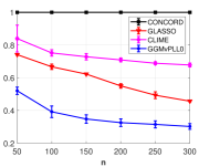
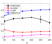
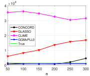
Figure 1: Comparison for the banded precision model in Section 5.1.2 with $k=6$.

Scenario 2, Uniform Sparsity: Here we choose $n\in\{50,\ldots,300\}$ and set the condition number to 200, and the row/column sparsity to $k\in\{5,10\}$ (i.e., $\|\bm{\Theta}^{*}\|_{0}\approx kp$). The results for $k=5$ are shown in Figure 2 and the results for $k=10$ can be found in Figure 3. Overall, it can be seen that our proposed estimator provides good estimation and support recovery performance. Moreover, our estimator is sparse, specially compared to CLIME and GLASSO. Another observation is that increasing the sparsity level leads to worse statistical performance, which is expected.

Estimation Error	MCC	NNZ

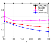
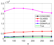
Figure 2: Comparison for the uniform sparsity model in Section 5.1.2 with $k=5$ and $p=200$.

Estimation Error	MCC	NNZ

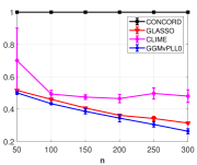
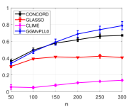
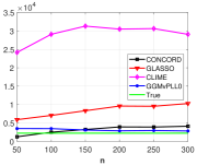
Figure 3: Comparisons for the uniform sparsity model in Section 5.1.2 with $k=10$ and $p=200$.

Finally, we consider some high-dimensional settings with larger values of $p$. We set $p=3000$, $k=10$ and we let the condition number to be 150. Only GraphL0BnB and GLASSO seem to scale to these instances. The results for this case are shown in Figure 4. We see that GraphL0BnB leads to almost-perfect support recovery for $n\approx 1000$ while providing better estimation performance compared to GLASSO. Moreover, GLASSO incurs a fairly large number of false positives and has a dense support, as observed before.

Estimation Error	MCC	NNZ

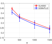
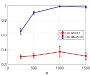
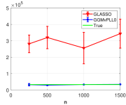
Figure 4: Comparison for the uniforms sparsity model in Section 5.1.2 with $k=10$ and $p=3000$.

5.2 A downstream application in portfolio optimization

We consider an application of sparse GGM in finance in the context of portfolio optimization. We use data on stock returns extracted from Yahoo! Finance from 2005 to 2019 for 1452 companies. Given the data, we consider the well-known problem in portfolio optimization: we select a portfolio that leads to maximum returns and minimum risk over the portfolio (Markowitz 1952). Given the returns data matrix $\bm{X}\in\mathbb{R}^{n\times p}$ and portfolio weights $\bm{w}\in\mathbb{R}^{p}_{\geq 0}$ with $\sum_{i=1}^{p}w_{i}=1$, the values of returns and risk are defined as

$$r=\sum_{i=1}^{n}(\bm{Xw})_{i},\quad\sigma=\sqrt{\text{VAR}(\bm{Xw})},$$ (28)

respectively, where VAR denotes the variance of the vector. To select the optimal portfolio, we solve the quadratic portfolio selection problem:

$$\min_{\bm{w}}~{}\bm{w}^{\top}\bm{\Sigma}_{X}\bm{w}~{}~{}~{}\text{s.t.}~{}~{}~{}\bm{w}\in\mathbb{R}_{\geq 0}^{p},~{}~{}\sum_{i=1}^{p}w_{i}=1~{}~{}$$ (29)

where $\bm{\Sigma}_{X}$ is an estimate of the covariance matrix. We explore different GGM methods on $\bm{X}$ to estimate $\hat{\bm{\Theta}}$ and use $\hat{\bm{\Theta}}^{-1}$ as an estimate of the covariance matrix. Then, after selecting the portfolio weights by solving (29), we calculate the returns and risk on a held-out test set of data points. For more details on the setup, see Khare et al. (2015).
We consider two cases. In the first case, we select the top 100 stocks with highest variance over time. Then, we use sparse GGM methods to estimate $\bm{\Sigma}_{X}$ and select the optimal portfolio using 1000 training data points and 500 validation points. Then, we use 1000 test data points to calculate the returns and risk. The average results for 20 selections of train/validation/test data are reported in Table 2 (the runtime for GraphL0BnB is to MIP gap of $5\%$). Overall, we see that our method provides the highest return. In terms of risk, GLASSO has a lower risk compared to our method, and our method leads to lower risk compared to other methods. We note that GraphL0BnB is more sparse than GLASSO. Compared to CONCORD, our method is more dense but has higher returns and lower risk. Overall, our method is performing well both statistically and computationally.

Table 2: Simulation results for the real dataset with top-100 and full stocks in Section 5.2.

	top-100				full data ($p=1452$)
	GraphL0BnB	GLASSO	CONCORD	CLIME	GraphL0BnB	GLASSO
Returns	$25.02$	$24.98$	$24.87$	$24.50$	8.96	2.50
Risk	$0.38$	$0.34$	$0.41$	$0.47$	0.36	0.20
$\|\hat{\bm{\Theta}}\|_{0}$	$2398$	$3060$	$107$	$3369$	27055	114450
Runtime	19.02	0.42	12.63	44.11	459	1470

Next, we use all stocks in the dataset ($p=1452$) and repeat the same experiment. In this case, we show results from only our method and GLASSO reported in Table 2. (Other methods faced numerical issues). Overall, our method provides a considerably higher value of return, while providing better returns to risk ratio. This is while our solution is more sparse and our algorithm is faster, showing that our estimator is superior in terms of statistical and computational performance.

6 Conclusion

We propose GraphL0BnB—a new estimator for the sparse GGM problem based on an $\ell_{0}$-regularized version of the pseudo-likelihood function. Our estimator is given by the solution of a mixed integer convex program. We propose a global optimization framework to obtain optimal solutions to the MIP using a custom branch-and-bound solver where we use specialized first-order methods to solve the convex problems at the node relaxations. We also present fast approximate solutions for the MIP which is of independent interest. We demonstrate that our proposed BnB framework can deliver near-optimal solutions with dual bounds for sparse instances with $n\approx 500$ samples and $p\approx 10,000$ features (i.e., around $50\times 10^{6}$ binary variables) in less than an hour. We also discuss the statistical properties of our estimator and derive estimation error and variable selection guarantees that generally match or improve upon existing theoretical guarantees for other sparse GGM methods. Our numerical experiments on synthetic and financial data show promising statistical and computational performance of our proposal.

Appendix A Computation: Additional Technical Details

A.1 Properties and optimization oracles related to regularizers

We discuss some technical details related to our coordinate descent algorithm.

In Sections A.1.1 and A.1.4, we first present the derivations related to updates (18) and (19), and we reduce the off-diagonal update (19) to a proximal operator computation problem. In Sections A.1.2 and A.1.3, we derive closed-form expressions of the proximal operators for the node/root relaxation subproblems (14) and the incumbent solving problem (7).

A.1.1 Off-diagonal update

We show that the update of $\hat{\theta}_{ij}$ in line 3 of Algorithm 1 is given by (18). For any $i<j$ and $h_{ij}$, we have

$$~{}F(\hat{\bm{\Theta}}-\hat{\theta}_{ij}\bm{E}_{ij}-\hat{\theta}_{ij}\bm{E}_{ji}+\theta_{ij}\bm{E}_{ij}+\theta_{ij}\bm{E}_{ji})$$

$$= ~{}\text{Const}+\frac{1}{\hat{\theta}_{ii}}\lVert\tilde{\bm{X}}\hat{\bm{\theta}}_{i}-\hat{\theta}_{ij}\tilde{\bm{x}}_{j}+\theta_{ij}\tilde{\bm{x}}_{j}\rVert^{2}+\frac{1}{\hat{\theta}_{jj}}\lVert\tilde{\bm{X}}\hat{\bm{\theta}}_{j}-\hat{\theta}_{ij}\tilde{\bm{x}}_{i}+\theta_{ij}\tilde{\bm{x}}_{i}\rVert^{2}+h_{ij}(\theta_{ij})$$

$$\overset{(a)}{=} ~{}\text{Const}+\frac{1}{\hat{\theta}_{ii}}\lVert\bm{r}_{i}-\hat{\theta}_{ij}\tilde{\bm{x}}_{j}+\theta_{ij}\tilde{\bm{x}}_{j}\rVert^{2}+\frac{1}{\hat{\theta}_{jj}}\lVert\bm{r}_{j}-\hat{\theta}_{ij}\tilde{\bm{x}}_{i}+\theta_{ij}\tilde{\bm{x}}_{i}\rVert^{2}+h_{ij}(\theta_{ij})$$

$$\overset{(b)}{=} ~{}\text{Const}+\frac{\lVert\tilde{\bm{x}}_{j}\rVert^{2}}{\hat{\theta}_{ii}}\theta_{ij}^{2}+\frac{2\tilde{\bm{x}}_{j}^{\top}(\bm{r}_{i}-\hat{\theta}_{ij}\tilde{\bm{x}}_{j})}{\hat{\theta}_{ii}}\theta_{ij}+\frac{\lVert\tilde{\bm{x}}_{i}\rVert^{2}}{\hat{\theta}_{jj}}\theta_{ij}^{2}+\frac{2\tilde{\bm{x}}_{i}^{\top}(\bm{r}_{j}-\hat{\theta}_{ij}\tilde{\bm{x}}_{i})}{\hat{\theta}_{jj}}\theta_{ij}+h_{ij}(\theta_{ij})$$

$$\overset{(c)}{=} ~{}\text{Const}+a_{ij}\theta_{ij}^{2}+b_{ij}\theta_{ij}+h_{ij}(\theta_{ij})$$

where “Const” denotes the constant terms (i.e., not depending on the optimization variable $\theta_{ij}$) and may vary from one line to another. Above, $(a)$ uses the definition of $\bm{r}_{i}=\tilde{\bm{X}}\hat{\bm{\theta}}_{i}$, $(b)$ expands the squared norm and moves the constant terms into Const, and $(c)$ is due to $v_{i}=\lVert\tilde{\bm{x}}_{i}\rVert^{2}$ and the definitions of $a_{ij}$ and $b_{ij}$.

In fact, the above update can be expressed using the proximal operator [Beck, 2017] for the regularizer $h_{ij}$ under some scaling as we discuss below. For a lower-semicontinuous function $h$, we let

$$\mathcal{Q}_{h}(a,b)=\arg\min_{\theta}~{}a\theta^{2}+b\theta+h(\theta),$$ (A.1)

and denote the proximal operator

$$\mathrm{prox}_{h}(\tilde{\theta})=\arg\min_{\theta}~{}\frac{1}{2}(\theta-\tilde{\theta})^{2}+h(\theta).$$ (A.2)

One can verify that

$$\mathcal{Q}_{h}(a,b)=\mathrm{prox}_{\frac{1}{2a}h}\left(-\frac{b}{2a}\right).$$ (A.3)

According to (A.3), it suffices to investigate how to compute the proximal operators for the regularizers. Below we present closed-form expressions for the proximal operators arising from the different regularizers considered in Section 3.3.

A.1.2 Regularizers for convex relaxations (node and root subproblems)

The results here extend those discussed in Hazimeh et al. [2022].

Interval relaxation: Recall that when $\underline{z}=0,\bar{z}=1$, the regularizer $g$ becomes

$$\psi(\theta;\lambda_{0},\lambda,M)=\min_{z,s}~{}\lambda_{0}z+\lambda_{2}s,~{}~{}\text{s.t.}~{}~{}sz\geq\theta^{2},~{}|\theta|\leq Mz,~{}z\in[0,1].$$

We summarize different cases of $\psi$ in Table A.1 (see also (13) in main paper).

Table A.1: Summary of different regimes and cases of $\psi$

Regime	Range of $|\theta|$	$\psi(\theta;\lambda_{0},\lambda_{2},M)$	$z^{*}$	$s^{*}$
$\sqrt{\lambda_{0}/\lambda_{2}}\leq M$	$[0,\sqrt{\lambda_{0}/\lambda_{2}})$	$2\sqrt{\lambda_{0}\lambda_{2}}|\theta|$	$\sqrt{\lambda_{2}/\lambda_{0}}|\theta|$	$\sqrt{\lambda_{0}/\lambda_{2}}|\theta|$
	$(\sqrt{\lambda_{0}/\lambda_{2}},M]$	$\lambda_{0}+\lambda_{2}\theta^{2}$	$1$	$\theta^{2}$
	$(M,\infty)$	$\infty$	$\varnothing$	$\varnothing$
$\sqrt{\lambda_{0}/\lambda_{2}}>M$	$[0,M]$	$(\lambda_{0}/M+\lambda_{2}M)|\theta|$	$|\theta|/M$	$|\theta|M$
	$(M,\infty)$	$\infty$	$\varnothing$	$\varnothing$

Given non-negative parameters $\lambda$ and $M$, we define the boxed soft-thresholding operator $\mathcal{T}:\mathbb{R}\to\mathbb{R}$ as follows:

$$\mathcal{T}(x;\lambda,M)=\left\{\begin{array}[]{ll}0&~{}\text{if}~{}|x|\leq\lambda\\ (|x|-\lambda)\operatorname*{sign}(x)&~{}\text{if}~{}\lambda\leq|x|\leq\lambda+M\\ M\operatorname*{sign}(x)&~{}\text{otherwise.}\end{array}\right.$$ (A.4)

Note that $\mathcal{T}(x;\lambda,M)$ is the proximal operator for the boxed $\ell_{1}$ regularizer

$$h(x)=\lambda|x|+\chi\{|x|\leq M\}.$$

Then, according to Hazimeh et al. [2022], the proximal operator of $\psi$ is given by

$$\mathrm{prox}_{\psi}(\tilde{\theta};\lambda_{0},\lambda_{2},M) =\arg\min_{\theta}~{}\frac{1}{2}(\theta-\tilde{\theta})^{2}+\psi(\theta;\lambda_{0},\lambda_{2},M)$$ (A.5)

$$=\left\{\begin{array}[]{ll}\mathcal{T}(\tilde{\theta};2\sqrt{\lambda_{0}\lambda_{2}},M)&~{}\text{if}~{}|\tilde{\theta}|\leq 2\sqrt{\lambda_{0}\lambda_{2}}+\sqrt{\lambda_{0}/\lambda_{2}}~{}\text{and}~{}\sqrt{\lambda_{0}/\lambda_{2}}\leq M\\ \mathcal{T}(\tilde{\theta}/(1+2\lambda_{2});0,M)&~{}\text{if}~{}|\tilde{\theta}|>2\sqrt{\lambda_{0}\lambda_{2}}+\sqrt{\lambda_{0}/\lambda_{2}}~{}\text{and}~{}\sqrt{\lambda_{0}/\lambda_{2}}\leq M\\ \mathcal{T}(\tilde{\theta};\lambda_{0}/M+\lambda_{2}M,M)&~{}\text{if}~{}\sqrt{\lambda_{0}/\lambda_{2}}>M.\end{array}\right.$$ (A.9)

Based on this, we define the following quadratic minimization oracle

$$\mathcal{Q}_{\psi}(a,b;\lambda_{0},\lambda_{2},M):=\arg\min_{x}~{}ax^{2}+bx+\psi(x;\lambda_{0},\lambda_{2},M)=\mathrm{prox}_{\psi}\left(-\frac{b}{2a};\frac{\lambda_{0}}{2a},\frac{\lambda_{2}}{2a},M\right).$$ (A.10)

Fixed $z$: Recall that when $\underline{z}=\bar{z}=z\in\{0,1\}$, the regularizer $g$ becomes $\varphi$ in (16), i.e.

$$\varphi(\theta;z,\lambda_{0},\lambda_{2},M) :=\min_{s}~{}~{}\lambda_{0}z+\lambda_{2}s$$

$$~{}~{}~{}~{}~{}~{}\text{s.t.}~{}~{}sz\geq\theta^{2},|\theta|\leq Mz,z\in[0,1]$$

$$=\left\{\begin{array}[]{ll}0&~{}\text{if}~{}z=0~{}\text{and}~{}|\theta|=0\\ \infty&~{}\text{if}~{}z=0~{}\text{and}~{}|\theta|>0\\ \lambda_{0}+\lambda_{2}\theta^{2}&~{}\text{if}~{}z=1~{}\text{and}~{}|\theta|\leq M\\ \infty&~{}\text{if}~{}z=1~{}\text{and}~{}|\theta|>M,\end{array}\right.$$ (A.15)

and its corresponding proximal operator is

$$\mathrm{prox}_{\varphi}(\tilde{\theta};z,\lambda_{0},\lambda_{2},M) =\arg\min_{\theta}~{}\frac{1}{2}(\theta-\tilde{\theta})^{2}+\varphi(\theta;z,\lambda_{0},\lambda_{2},M)$$

$$=\left\{\begin{array}[]{ll}0&~{}\text{if}~{}z=0\\ \mathcal{T}(\tilde{\theta}/(1+2\lambda_{2});0,M)&~{}\text{if}~{}z=1.\end{array}\right.$$ (A.18)

Based on this, we define the following regularized quadratic optimization problem:

$$\mathcal{Q}_{\varphi}(a,b;z,\lambda_{0},\lambda_{2},M):= \arg\min_{x}~{}ax^{2}+bx+\varphi(x;z,\lambda_{0},\lambda_{2},M)$$ (A.19)

$$= \mathrm{prox}_{\varphi}\left(-\frac{b}{2a};z,\frac{\lambda_{0}}{2a},\frac{\lambda_{2}}{2a},M\right).$$

A.1.3 $\ell_{0}\ell_{2}$ regularizers

We derive the closed-form expression for the proximal operator corresponding to the $\ell_{0}\ell_{2}$ regularizer (i.e., a weighted sum of the $\ell_{0}$ and squared $\ell_{2}$ penalty):

$$h(\theta)=\lambda_{0}\bm{1}\{\theta\neq 0\}+\lambda_{2}\theta^{2}+\chi\{|\theta|\leq M\},$$

where $M\in(0,\infty]$, and $M$ could take the value $\infty$.

The proximal operator of $h$ is

$$\mathrm{prox}_{h}(\tilde{\theta};\lambda_{0},\lambda_{2},M)=\arg\min_{|\theta|\leq M}q(\theta):=\frac{1}{2}(\theta-\tilde{\theta})^{2}+\lambda_{0}\bm{1}\{\theta\neq 0\}+\lambda_{2}\theta^{2}.$$

When $\theta=0$, we have $q(0)=(1/2)\tilde{\theta}^{2}$; when $\theta\neq 0$, we have $q(\theta)=\lambda_{0}+\lambda_{2}\theta^{2}+\frac{1}{2}(\theta-\tilde{\theta})^{2}$, which is minimized at $\theta^{\prime}=\min\{|\tilde{\theta}|/(1+2\lambda_{2}),M\}\operatorname*{sign}(\tilde{\theta})$.

Without loss of generality, we assume $\tilde{\theta}>0$. If $\frac{\tilde{\theta}}{1+2\lambda_{2}}>M$, then $\theta^{\prime}=M$, and

$$q(\theta^{\prime})=\lambda_{0}+\lambda_{2}M^{2}+\frac{1}{2}(M-\tilde{\theta})^{2}.$$

The root of $q(\theta^{\prime})=q(0)$ is $\tilde{\theta}=(\frac{1}{2}+\lambda_{2})M+\frac{\lambda_{0}}{M}$.

If, on the other hand, $\frac{\tilde{\theta}}{1+2\lambda_{2}}\leq M$, then $\theta^{\prime}=\frac{\tilde{\theta}}{1+2\lambda_{2}}$, and

$$q(\theta^{\prime})=\lambda_{0}+\frac{\lambda_{2}\tilde{\theta}^{2}}{1+2\lambda_{2}}.$$

The root of $q(\theta^{\prime})=q(0)$ is $\tilde{\theta}=\sqrt{2\lambda_{0}(1+2\lambda_{2})}$.

Putting together the pieces, we obtain the following closed-form expression for the proximal operator corresponding to the $\ell_{0}\ell_{2}$ regularizer

$$\mathrm{prox}_{h}(\tilde{\theta};\lambda_{0},\lambda_{2},M)= \arg\min_{|\theta|\leq M}q(\theta)$$ (A.20)

$$= \left\{\begin{array}[]{ll}\{M\operatorname*{sign}(\tilde{\theta})\},&\text{if}~{}|\tilde{\theta}|>\max\left\{(\frac{1}{2}+\lambda_{2})M+\frac{\lambda_{0}}{M},(1+2\lambda_{2})M\right\}\\ \{0,M\operatorname*{sign}(\tilde{\theta})\},&\text{if}~{}|\tilde{\theta}|=(\frac{1}{2}+\lambda_{2})M+\frac{\lambda_{0}}{M}>(1+2\lambda_{2})M\\ \{0\},&\text{if}~{}|\tilde{\theta}|\in\left((1+\lambda_{2})M,(\frac{1}{2}+\lambda_{2})M+\frac{\lambda_{0}}{M}\right)\\ \{\frac{\tilde{\theta}}{1+2\lambda_{2}}\},&\text{if}~{}|\tilde{\theta}|\in\left(\sqrt{2\lambda_{0}(1+2\lambda_{2})},(1+2\lambda_{2})M\right]\\ \{0,\frac{\tilde{\theta}}{1+2\lambda_{2}}\},&\text{if}~{}|\tilde{\theta}|=\sqrt{2\lambda_{0}(1+2\lambda_{2})}\leq(1+2\lambda_{2})M\\ \{0\},&\text{if}~{}|\tilde{\theta}|<\min\{\sqrt{2\lambda_{0}(1+2\lambda_{2})},(1+2\lambda_{2})M\}.\end{array}\right.$$

Note that in the special case when $M=\infty$, (A.20) (i.e., the last three conditions) recovers the closed-form expression for $\ell_{0}\ell_{2}$ regularizer provided in Hazimeh and Mazumder [2020].

A.1.4 Diagonal update

We show that the update of $\hat{\theta}_{ii}$ in line 6 of Algorithm 1 is given by (19). For any $i$, we have

$$F(\hat{\bm{\Theta}}-\hat{\theta}_{ii}\bm{E}_{ii}+\theta_{ii}\bm{E}_{ii}) =\text{Const}-\log\theta_{ii}+\frac{1}{\theta_{ii}}\lVert\tilde{\bm{X}}\hat{\bm{\theta}}_{i}-\hat{\theta}_{ii}\tilde{\bm{x}}_{i}+\theta_{ii}\tilde{\bm{x}}_{i}\rVert^{2}$$

$$\overset{(a)}{=}\text{Const}-\log\theta_{ii}+\frac{1}{\theta_{ii}}\lVert\bm{r}_{i}-\hat{\theta}_{ii}\tilde{\bm{x}}_{i}+\theta_{ii}\tilde{\bm{x}}_{i}\rVert^{2}$$

$$\overset{(b)}{=}\text{Const}-\log\theta_{ii}+\frac{1}{\theta_{ii}}(\lVert\bm{e}_{i}\rVert^{2}+2\theta_{ii}\bm{e}_{i}^{\top}\tilde{\bm{x}}_{i}+\theta_{ii}^{2}\lVert\tilde{\bm{x}}_{i}\rVert^{2})$$

$$\overset{(c)}{=}\text{Const}-\log\theta_{ii}+\frac{\lVert\bm{e}_{i}\rVert^{2}}{\theta_{ii}}+\theta_{ii}v_{i},$$

where “Const” denotes the constant terms (similar notation as earlier); $(a)$ and $(b)$ uses the definitions of $\bm{r}_{i}=\tilde{\bm{X}}\hat{\bm{\theta}}_{i}$ and $\bm{e}_{i}=\bm{r}_{i}-\hat{\theta}_{ii}\tilde{\bm{x}}_{i}$, and $(c)$ is due to $v_{i}=\lVert\tilde{\bm{x}}_{i}\rVert^{2}$ and $2\bm{e}_{i}^{\top}\tilde{\bm{x}}_{i}$ absorbed into Const.

Since the function

$$\theta_{ii}\mapsto F(\hat{\bm{\Theta}}-\hat{\theta}_{ii}\bm{E}_{ii}+\theta_{ii}\bm{E}_{ii})$$

is convex in $\theta_{ii}$, by considering the first-order optimality condition and taking the positive root, we get

$$\arg\min_{\theta_{ii}}F(\hat{\bm{\Theta}}-\hat{\theta}_{ii}\bm{E}_{ii}+\theta_{ii}\bm{E}_{ii})=\arg\min_{\theta}-\log\theta+\theta v_{i}+\frac{\lVert\bm{e}_{i}\rVert^{2}}{\theta}=\frac{1+\sqrt{1+4v_{i}\lVert\bm{e}_{i}\rVert^{2}}}{2v_{i}}.$$

A.2 Convergence guarantee of Algorithm 1

In this section, we present a general convergence statement for Algorithm 1 that applies to the unified formulation (17), with the following assumption on $h_{ij}$:

Assumption 1.

Assume that for each $1\leq i<j\leq p$, $h_{ij}(\theta)$ is convex in $\theta$. In addition, there exist two constants $c_{1},c_{2}\geq 0$ with $c_{1}+c_{2}>0$, such that for any $1\leq i<j\leq p$, we have

$$h_{ij}(\theta)\geq\min\{c_{1}|\theta|,c_{2}\theta^{2}\}.$$

It is easy to see that the usual $\ell_{1}$, $\ell_{2}$ (squared) penalties and their nonegative weighted combinations satisfy Assumption 1. The following proposition states that the relaxation regularizer $g$ (see definition (14)) also satisfies this assumption.

Proposition A.1.

For any $\underline{z}_{ij}\leq\bar{z}_{ij}\in\{0,1\}$, $g(\theta;\lambda_{0},\lambda_{2},M,\underline{z}_{ij},\bar{z}_{ij})$ satisfies Assumption 1 with $c_{1}=2\sqrt{\lambda_{0}\lambda_{2}},c_{2}=0$.

Proof..

Based on the definition of $\varphi$ and $\psi$ in different cases, using the inequality $a^{2}+b^{2}\geq 2ab$, one can verify that $\psi(\theta;\lambda_{0},\lambda_{2},M)\geq 2\sqrt{\lambda_{0}\lambda_{2}}|\theta|$ and $\varphi(\theta;z,\lambda_{0},\lambda,M)\geq 2\sqrt{\lambda_{0}\lambda_{2}}|\theta|$. ∎

Lemma A.1.

Under Assumption 1, given any $U\geq F^{*}=\min_{\bm{\Theta}\in\mathbb{S}^{p}}F(\bm{\Theta})$, there exist constants $u_{\theta}\geq l_{\theta}>0$ and $u_{r}>0$, such that for any $\bm{\Theta}$ with $F(\bm{\Theta})\leq U$, we have

$$l_{\theta}\leq\theta_{ii}\leq u_{\theta}\quad\text{and}\quad\lVert\tilde{\bm{X}}\bm{\theta}_{i}\rVert\leq u_{r}$$

for all $i\in[p]$.

Proof of Lemma A.1..

For any $\bm{\Theta}$ such that $F(\bm{\Theta})\leq U$, let $k=\arg\max_{i\in[p]}\theta_{ii}$. Then, we have

$$U \geq F(\bm{\Theta})$$ (A.21)

$$=\sum_{i=1}^{p}\left(-\log\theta_{ii}+\frac{1}{\theta_{ii}}\lVert\tilde{\bm{X}}\bm{\theta}_{i}\rVert^{2}\right)+\sum_{i<j}h_{ij}(\theta_{ij})$$

$$\geq-p\log\theta_{kk}+\frac{1}{\theta_{kk}}\lVert\tilde{\bm{X}}\bm{\theta}_{k}\rVert^{2}+\sum_{i\neq k}\min\{c_{1}|\theta_{ik}|,c_{2}\theta_{ik}^{2}\},$$

where the last line is because (i) $-\log\theta_{ii}\geq-\log\theta_{kk}$ by definition of $k$; (ii) by Assumption 1, $h_{ij}(\theta_{ij})\geq\min\{c_{1}|\theta_{ij}|,c_{2}\theta_{ij}^{2}\}\geq 0$; (iii) $\frac{1}{\theta_{ii}}\lVert\tilde{\bm{X}}\bm{\theta}_{i}\rVert^{2}$ is nonnegative for any $i\neq k$.

Now define $\bm{\beta}_{k}\in\mathbb{R}^{p}$, with $\beta_{kk}=0$ and $\beta_{ki}=-\theta_{ik}/\theta_{kk}$, then we can rewrite (A.21) into

$$U \geq-p\log\theta_{kk}+\frac{1}{\theta_{kk}}\lVert\theta_{kk}\tilde{\bm{x}}_{k}-\tilde{\bm{X}}\theta_{kk}\bm{\beta}_{k}\rVert^{2}+\sum_{i\neq k}\min\{c_{1}|\theta_{ik}|,c_{2}\theta_{ik}^{2}\}$$

$$=-p\log\theta_{kk}+\theta_{kk}\lVert\tilde{\bm{x}}_{k}-\tilde{\bm{X}}\bm{\beta}_{k}\rVert^{2}+\sum_{i\neq k}\min\{c_{1}\theta_{kk}|\beta_{ki}|,c_{2}\theta_{kk}^{2}\beta_{ki}^{2}\}$$

$$\overset{(A)}{\geq}-p\log\theta_{kk}+\theta_{kk}\max\left\{\frac{1}{2}\lVert\tilde{\bm{x}}_{k}\rVert^{2}-\lVert\tilde{\bm{X}}\bm{\beta}_{k}\rVert^{2},0\right\}+\sum_{i\neq k}\min\{c_{1}\theta_{kk}|\beta_{ki}|,c_{2}\theta_{kk}^{2}\beta_{ki}^{2}\}$$

$$\overset{(B)}{\geq}-p\log\theta_{kk}+\theta_{kk}\max\left\{\frac{1}{2}s_{\min}-L_{\tilde{\bm{X}}}^{2}\lVert\bm{\beta}_{k}\rVert^{2},0\right\}+\sum_{i\neq k}\min\{c_{1}\theta_{kk}|\beta_{ki}|,c_{2}\theta_{kk}^{2}\beta_{ki}^{2}\},$$ (A.22)

where inequality $(A)$ uses the fact that $\lVert\bm{a}+\bm{b}\rVert^{2}\leq 2(\lVert\bm{a}\rVert^{2}+\lVert\bm{b}\rVert^{2})$ with $\bm{a}=\tilde{\bm{x}}_{k}-\tilde{\bm{X}}\bm{\beta}_{k}$ and $\bm{b}=\tilde{\bm{X}}\bm{\beta}_{k}$; in inequality $(B)$, we define $s_{\min}=\min_{i}v_{i}=\min_{i}\lVert\tilde{\bm{x}}_{i}\rVert^{2}>0$ and $L_{\tilde{\bm{X}}}=\lVert\tilde{\bm{X}}\rVert$.

Now if $\lVert\bm{\beta}_{k}\rVert\leq\epsilon:=L_{\tilde{\bm{X}}}\sqrt{s_{\min}}/2$, then it follows from (A.22) that

$$-p\log\theta_{kk}+\frac{1}{4}s_{\min}\theta_{kk}\leq U,$$

from which we can deduce that there exists $u_{1}>0$ such that $\theta_{kk}\leq u_{1}$. On the other hand, if $\lVert\bm{\beta}_{k}\rVert>\epsilon$, then there exists a $j$ such that $|\beta_{kj}|\geq\epsilon/\sqrt{p}$. Again by (A.22), we have

$$-p\log\theta_{kk}+\min\{c_{1}\theta_{kk}\epsilon/\sqrt{p},c_{2}\theta_{kk}\epsilon^{2}/p\}\leq U,$$

and thus there exists $u_{2}>0$, such that $\theta_{kk}\leq u_{2}$. Therefore, $\theta_{kk}=\max_{i}\theta_{ii}\leq\max\{u_{1},u_{2}\}$, and by taking $u_{\theta}=\max\{u_{1},u_{2}\}$, we get the upper bound on $\theta_{ii}$’s.

As for the lower bound on $\theta_{ii}$, let $\ell=\arg\min_{i}\theta_{ii}$. By nonnegativity of $\frac{1}{\theta_{ii}}\lVert\tilde{\bm{X}}\bm{\theta}_{i}\rVert^{2}$ and $h_{ij}$’s, we have

$$U\geq-\sum_{i=1}^{p}\log\theta_{ii}=-\log\theta_{\ell\ell}-\sum_{i\neq\ell}\log\theta_{ii}\geq-\log\theta_{\ell\ell}-(p-1)\log u_{\theta}.$$

Therefore, $\theta_{\ell\ell}=\min_{i}\theta_{ii}\geq\exp(-M-(p-1)\log u_{\theta})$, and we obtain the lower bound $l_{\theta}=\exp(-M-(p-1)\log u_{\theta})$.

To obtain the upper bound on $\lVert\tilde{\bm{X}}\bm{\theta}_{i}\rVert$, again by nonnegativity of $\frac{1}{\theta_{ii}}\lVert\tilde{\bm{X}}\bm{\theta}_{i}\rVert^{2}$ and $h_{ij}$’s, we have for any $j$:

$$U\geq-\sum_{i=1}^{p}\log\theta_{ii}+\frac{1}{\theta_{jj}}\lVert\tilde{\bm{X}}\bm{\theta}_{j}\rVert^{2}=-p\log u_{\theta}+\frac{1}{u_{\theta}}\lVert\tilde{\bm{X}}\bm{\theta}_{j}\rVert^{2}.$$

Therefore, $\lVert\tilde{\bm{X}}\bm{\theta}_{j}\rVert^{2}\leq u_{\theta}(U+p\log u_{\theta})$, and we obtain the upper bound as stated in the lemma with $u_{r}=\sqrt{u_{\theta}(U+p\log u_{\theta})}$. ∎

Corollary 1.

Let us denote:

$$f(\bm{\Theta})=\sum_{i=1}^{p}\left(-\log\theta_{ii}+\frac{1}{\theta_{ii}}\lVert\tilde{\bm{X}}\bm{\theta}_{i}\rVert^{2}\right).$$

Under Assumption 1, given any $F^{(0)}\geq F^{*}=\min_{\bm{\Theta}\in\mathbb{S}^{p}}F(\bm{\Theta})$, let us define $\Xi=\{\bm{\Theta}\in\mathbb{S}^{p}:F(\bm{\Theta})\leq F^{(0)}\}\subseteq\mathbb{S}^{p}$. Then, over $\Xi$,

1. There exists a scalar $L>0$ such that $\nabla f$ is $L$-Lipschitz.

2. There exist scalars $L_{ij}>0$ such that $\nabla f$ is $\{L_{ij}\}$-coordinatewise Lipschitz. That is, for $\bm{\Theta}\in\Xi$, the function

   $$x\mapsto\nabla_{\theta_{ij}}f(\bm{\Theta}+x(\bm{E}_{ij}+\bm{E}_{ji})),~{}~{}~{}\text{with}~{}~{}~{}\bm{\Theta}+x(\bm{E}_{ij}+\bm{E}_{ji})\in\Xi$$

   is $L_{ij}$-Lipschitz where $\bm{E}_{ij}$ denotes the matrix with coordinate $(i,j)$ equal to one and other coordinates set to zero.

3. There exist constants $\mu_{ij}>0$ such that the objective function $F(\bm{\Theta})$ in (17) is $\{\mu_{ij}\}$-coordinatewise strongly convex. That is, for $\bm{\Theta}\in\Xi$, the function

   $$x\mapsto F(\bm{\Theta}+x(\bm{E}_{ij}+\bm{E}_{ji})),~{}~{}~{}\text{with}~{}~{}~{}\bm{\Theta}+x(\bm{E}_{ij}+\bm{E}_{ji})\in\Xi$$

   is $\mu_{ij}$ strongly convex.

Proof of Corollary 1..

We will show (b) and (c), and (a) follows from (b).

From the derivation of the off-diagonal update in Section A.1.1, we can easily see that the second derivative of $f$ with respect to the off-diagonal entry $\theta_{ij}$ (for any $i<j$) is given by

$$\nabla_{\theta_{ij}}^{2}f(\bm{\Theta})=\frac{v_{i}}{\theta_{jj}}+\frac{v_{j}}{\theta_{ii}}$$ (A.23)

with $v_{i}=\tilde{\bm{x}}_{i}^{\top}\tilde{\bm{x}}_{i}$.

From the derivation of the diagonal update in Section A.1.4, we see that the second derivative of $f$ with respect to a diagonal entry $\theta_{ii}$ (for any $i$) is given by

$$\nabla^{2}_{\theta_{ii}}f(\bm{\Theta})=\frac{1}{\theta_{ii}^{2}}+\frac{\lVert\tilde{\bm{X}}_{-i}\bm{\theta}_{i,-i}\rVert^{2}}{2\theta_{ii}^{2}}$$ (A.24)

where $\tilde{\bm{X}}_{-i}\in\mathbb{R}^{n\times(p-1)}$ is the data matrix $\tilde{\bm{X}}$ without the $i$-th column, and $\bm{\theta}_{i,-i}\in\mathbb{R}^{p-1}$ is the vector $\bm{\theta}_{i}$ without its $i$-th component.

Proof of Part (b) By Lemma A.1, we have $\theta_{ii}\geq l_{\theta}$, and it follows from (A.23) that $\nabla_{\theta_{ij}}^{2}f(\bm{\Theta})\leq(v_{i}+v_{j})/l_{\theta}$. Therefore, we have $\nabla f$ is $L_{ij}$-Lipschitz with respect to $\theta_{ij}$, where $L_{ij}=(v_{i}+v_{j})/l_{\theta}$.

Again by Lemma A.1, we have $\theta_{ii}\geq l_{\theta}$ and $\lVert\tilde{\bm{X}}\bm{\theta}_{i}\rVert^{2}\leq u_{r}^{2}$, and thus

$$\nabla_{\theta_{ii}}^{2}f(\bm{\Theta})= \frac{1}{\theta_{ii}^{2}}+\frac{\lVert\tilde{\bm{X}}\bm{\theta}_{i}-\theta_{ii}\tilde{\bm{x}}_{i}\rVert^{2}}{2\theta_{ii}^{2}}$$

$$\leq \frac{1+\lVert\tilde{\bm{X}}\bm{\theta}_{i}\rVert^{2}+\theta_{ii}^{2}\lVert\tilde{\bm{x}}_{i}\rVert^{2}}{\theta_{ii}^{2}}$$

$$\leq \frac{1+u_{r}^{2}}{l_{\theta}^{2}}+v_{i}.$$

Therefore, we have $\nabla f$ is $L_{ii}$-Lipschitz with respect to $\theta_{ii}$, where $L_{ii}=(1+u_{r}^{2})/l_{\theta}^{2}+v_{i}$.

Proof of Part (c) By Lemma A.1, we have $\theta_{ii}\leq u_{\theta}$, so $\nabla_{\theta_{ij}}^{2}f(\bm{\Theta})\geq(v_{i}+v_{j})/u_{\theta}$. Therefore, we have $F$ is $\mu_{ij}$-strongly convex with respect to every coordinate $\theta_{ij}$, where $\mu_{ij}=(v_{i}+v_{j})/u_{\theta}$.

Similarly, we have $F$ is $\mu_{ii}$-strongly convex with respect to $\theta_{ii}$ with $\mu_{ii}=1/u_{\theta}^{2}$. ∎

Theorem A.1.

Under Assumption 1, given any initialization $\bm{\Theta}^{(0)}$, let $\bm{\Theta}^{(t)}$ be the $t$-th iterate generated by Algorithm 1. Then there is a constant $C$ that depends on $\bm{\Theta}^{(0)}$, such that for any $t\geq 1$,

$$F(\bm{\Theta}^{(t)})-F^{*}\leq\frac{C}{t},$$

where $F^{*}=\min_{\bm{\Theta}\in\mathbb{S}^{p}}F(\bm{\Theta})$.

Proof of Theorem A.1..

Note that Algorithm 1 is a descent algorithm—the objective function decreases after each coordinate update. Therefore, we must have

$$F(\bm{\Theta}^{(t)})\leq F(\bm{\Theta}^{(0)}),$$

i.e. $\bm{\Theta}^{(t)}\in\{\bm{\Theta}:F(\bm{\Theta})\leq F(\bm{\Theta}^{(0)})\}$.

Since Assumption 1 holds, invoking Corollary 1 with $F^{(0)}=F(\bm{\Theta}^{(0)})$, we get $f$ is coordinatewise Lipschitz and $F$ is coordinatewise strongly convex with some parameters depending on $F^{(0)}$, and thus on $\bm{\Theta}^{(0)}$. According to Hong et al. [2017], we get the sublinear rate of convergence of Algorithm 1, i.e.

$$F(\bm{\Theta}^{(t)})-F^{*}\leq\frac{C}{t},$$

where the constant $C$ depends on $\bm{\Theta}^{(0)}$. ∎

Remark 1.

According to Proposition A.1, the regularizers $g(\theta_{ij};\lambda_{0},\lambda_{2},M,\underline{z}_{ij},\bar{z}_{ij})$ in $F_{\mathsf{node}}$ satisfy Assumption 1, and thus Theorem A.1 applies to $F_{\mathsf{node}}$, which is exactly Theorem 1 in the main paper.

A.3 Dual bound

We first present a proof for Theorem 2 in Section A.3.1, deriving the Lagrangian dual of the node relaxation objective $F_{\mathsf{node}}$. We then provide a sketch of how to compute the convex conjugate of $\psi$ and $\varphi$ as two cases of $g$ in Section A.3.2. Finally, we provide the proof for Proposition 1 in Section A.3.3.

A.3.1 Proof of Theorem 2

We introduce auxiliary primal variables $\bm{r}_{i}=\tilde{\bm{X}}\bm{\theta}_{i}$ to rewrite Problem (14) as follows:

$$\min_{\bm{\Theta}\in\mathbb{S}^{p}}{} ~{}\sum_{i=1}^{p}(-\log\theta_{ii}+\frac{1}{\theta_{ii}}\lVert\bm{r}_{i}\rVert^{2})+\sum_{i<j}g(\theta_{ij};\lambda_{0},\lambda_{2},M,\underline{z}_{ij},\bar{z}_{ij})$$ (A.25)

  s.t. $$~{}\bm{r}_{i}=\tilde{\bm{X}}\bm{\theta}_{i},~{}\forall i\in[p].$$

By dualizing the constraints in (A.25), we can write the Lagrangian as

$$\mathcal{L}(\bm{\Theta},\bm{r};\bm{\nu})=\sum_{i=1}^{p}(-\log\theta_{ii}+\frac{1}{\theta_{ii}}\lVert\bm{r}_{i}\rVert^{2}+\langle\bm{\nu}_{i},\bm{r}_{i}-\tilde{\bm{X}}\bm{\theta}_{i}\rangle)+\sum_{i<j}g(\theta_{ij};\lambda_{0},\lambda_{2},M,\underline{z}_{ij},\bar{z}_{ij}).$$ (A.26)

The Lagrangian dual is given by $D(\bm{\nu})=\min_{\bm{\Theta}\in\mathbb{S}^{p}}\mathcal{L}(\bm{\Theta},\bm{r};\bm{\nu}).$ Since Slater’s condition holds [Bertsekas, 2016], we have by strong duality:

$$\min_{\bm{\Theta}\in\mathbb{S}^{p}}F_{\text{node}}(\bm{\Theta})=\max_{\bm{\nu}}D(\bm{\nu}).$$

Minimizing (A.26) with respect to $\bm{r}_{i}$, we get

$$\bm{r}_{i}=-\frac{\theta_{ii}}{2}\bm{\nu}_{i}.$$ (A.27)

Plugging this back to the Lagrangian (A.26), we get

$$\theta_{ii}=\arg\min_{\theta}~{}-\log\theta+\theta(-\lVert\bm{\nu}_{i}\rVert^{2}/4-\tilde{\bm{x}}_{i}^{\top}\bm{\nu}_{i}),$$

which yields

$$\theta_{ii}=\frac{1}{-\lVert\bm{\nu}_{i}\rVert^{2}/4-\tilde{\bm{x}}_{i}^{\top}\bm{\nu}_{i}}\quad\text{if}\quad-\lVert\bm{\nu}_{i}\rVert^{2}/4-\tilde{\bm{x}}_{i}^{\top}\bm{\nu}_{i}>0.$$ (A.28)

If $-\lVert\bm{\nu}_{i}\rVert^{2}/4-\tilde{\bm{x}}_{i}^{\top}\bm{\nu}_{i}\leq 0$, then $\theta_{ii}\to\infty$, and the minimum value is $-\infty$, which cannot be achieved.

As for $\theta_{ij}=\theta_{ji}$,

$$\theta_{ij}=\theta_{ji} =\arg\min_{\theta}~{}(-\tilde{\bm{x}}_{j}^{\top}\bm{\nu}_{i}-\tilde{\bm{x}}_{i}^{\top}\bm{\nu}_{j})\theta+g(\theta;\lambda_{0},\lambda_{2},M,\underline{z}_{ij},\bar{z}_{ij})$$

$$=\arg\max_{\theta}~{}(\tilde{\bm{x}}_{j}^{\top}\bm{\nu}_{i}+\tilde{\bm{x}}_{i}^{\top}\bm{\nu}_{j})\theta-g(\theta;\lambda_{0},\lambda_{2},M,\underline{z}_{ij},\bar{z}_{ij})$$

$$\in\partial g^{*}(\tilde{\bm{x}}_{j}^{\top}\bm{\nu}_{i}+\tilde{\bm{x}}_{i}^{\top}\bm{\nu}_{j};\lambda_{0},\lambda_{2},M,\underline{z}_{ij},\bar{z}_{ij}).$$ (A.29)

Therefore, plugging (A.27), (A.28) and (A.29) into the Lagrangian function (A.26), we get the Lagrangian dual problem:

$$\max_{\bm{\nu}}~{}D(\bm{\nu})=p+\sum_{i=1}^{p}\log(-\lVert\bm{\nu}_{i}\rVert^{2}/4-\tilde{\bm{x}}_{i}^{\top}\bm{\nu}_{i})-\sum_{i<j}g^{*}(\tilde{\bm{x}}_{j}^{\top}\bm{\nu}_{i}+\tilde{\bm{x}}_{i}^{\top}\bm{\nu}_{j};\lambda_{0},\lambda_{2},M,\underline{z}_{ij},\bar{z}_{ij}).$$ (A.30)

A.3.2 Computing the convex conjugates

Convex Conjugate of $\psi$: We consider the Fenchel conjugate $\psi^{*}$ of $\psi$:

$$\psi^{*}(\alpha;\lambda_{0},\lambda_{2},M) :=\sup_{\theta}~{}\alpha\theta-\psi(\theta;\lambda_{0},\lambda_{2},M).$$ (A.31)

According to Hazimeh et al. [2022], when $\sqrt{\lambda_{0}/\lambda_{2}}\leq M$,

$$\psi^{*}(\alpha;\lambda_{0},\lambda_{2},M)=\min_{\gamma}\left[\frac{(\gamma-\alpha)^{2}}{4\lambda_{2}}-\lambda_{0}\right]_{+}+M|\gamma|;$$ (A.32)

and when $\sqrt{\lambda_{0}/\lambda_{2}}>M$, we have

$$\psi^{*}(\alpha;\lambda_{0},\lambda_{2},M)=\min_{\mu}~{}M|\mu|\quad\text{s.t.}\quad|\alpha|-\mu\leq\lambda_{0}/M+\lambda_{2}M.$$ (A.33)

Table A.2 below summarizes different expressions for $\psi^{*}$:

Table A.2: Summary of different regimes and cases of $\psi^{*}$

Regime	Range of $|\alpha|$	$\psi^{*}(\alpha;\lambda_{0},\lambda_{2},M)$	$\theta^{*}\in\partial\psi^{*}(\alpha)$	$\gamma^{*}/\mu^{*}$
$\sqrt{\lambda_{0}/\lambda_{2}}\leq M$	$[0,2\sqrt{\lambda_{0}\lambda_{2}})$	$0$	$0$	$0$
	$(2\sqrt{\lambda_{0}\lambda_{2}},2\lambda_{2}M]$	$\frac{\alpha^{2}}{4\lambda_{2}}-\lambda_{0}$	$\frac{\alpha}{2\lambda_{2}}$	$0$
	$(2\lambda_{2}M,\infty)$	$M|\alpha|-(\lambda_{0}+\lambda_{2}M^{2})$	$M\operatorname*{sign}(\alpha)$	$\alpha-2M\lambda_{2}\operatorname*{sign}(\alpha)$
$\sqrt{\lambda_{0}/\lambda_{2}}>M$	$[0,\lambda_{0}/M+\lambda_{2}M]$	$0$	$0$	$0$
	$(\lambda_{0}/M+\lambda_{2}M,\infty)$	$M|\alpha|-(\lambda_{0}+\lambda_{2}M^{2})$	$M\operatorname*{sign}(\alpha)$	$|\alpha|-(\lambda_{0}/M+\lambda_{2}M)$

Convex conjugate of $\varphi$: We consider the Fenchel conjugate $\varphi^{*}$ of $\varphi$:

$$\varphi^{*}(\alpha;z,\lambda_{0},\lambda_{2},M):=\sup_{\theta}~{}\alpha\theta-\varphi(\theta;z,\lambda_{0},\lambda_{2},M).$$ (A.34)

In Table A.3, we summarize the expressions for $\varphi^{*}$

Table A.3: Summary of different regimes and cases of $\varphi^{*}$

Regime	Range of $|\alpha|$	$\varphi^{*}(\alpha;z,\lambda_{0},\lambda_{2},M)$	$\theta^{*}\in\partial\varphi^{*}(\alpha;z)$
$z=0$	$[0,\infty)$	$0$	$0$
$z=1,\lambda_{2}>0$	$[0,2\lambda_{2}M]$	$\frac{\alpha^{2}}{4\lambda_{2}}-\lambda_{0}$	$\frac{\alpha}{2\lambda_{2}}$
	$(2\lambda_{2}M,\infty)$	$M|\alpha|-(\lambda_{0}+\lambda_{2}M^{2})$	$M\operatorname*{sign}(\alpha)$
$z=1,\lambda_{2}=0$	$[0,\infty)$	$M|\alpha|-\lambda_{0}$	$M\operatorname*{sign}(\alpha)$

A.3.3 Proof of Proposition 1

To prove Proposition 1, we will need a couple of helper propositions A.2 and A.3

Proposition A.2.

Denote by

$$c(\lambda_{0},\lambda_{2},M)=\left\{\begin{array}[]{ll}2\sqrt{\lambda_{0}\lambda_{2}}&~{}\text{if}~{}\sqrt{\lambda_{0}/\lambda_{2}}\leq M\\ \lambda_{0}/M+\lambda_{2}M&~{}\text{otherwise.}\end{array}\right.$$ (A.35)

The following statements hold

1. $\mathrm{prox}_{\psi}(\tilde{\beta};\lambda_{0},\lambda_{2},M)=0~{}\iff~{}|\tilde{\beta}|\leq c(\lambda_{0},\lambda_{2},M)$

2. $\mathcal{Q}_{\psi}(a,b;\lambda_{0},\lambda_{2},M)=0~{}\iff~{}|b|\leq c(\lambda_{0},\lambda_{2},M)$

3. $\psi^{*}(\alpha;\lambda_{0},\lambda_{2},M)=0~{}\iff~{}|\alpha|\leq c(\lambda_{0},\lambda_{2},M)$

The proof of Proposition A.2 follows by using (A.5), (A.10) and Table A.2.

Before stating the next proposition A.3, we recall the definitions of $\hat{\mathcal{S}}$ and $\mathcal{F}_{1}$:

$$\hat{\mathcal{S}}=\{(i,j):i<j,\hat{\theta}_{ij}\neq 0\},\quad\text{and}\quad\mathcal{F}_{1}=\{(i,j):\underline{z}_{ij}=\bar{z}_{ij}=1\}.$$

Additionally, we define

$$\mathcal{F}_{0}=\{(i,j):\underline{z}_{ij}=\bar{z}_{ij}=0\}\quad\text{and}\quad\mathcal{R}=\{(i,j):\underline{z}_{ij}=0,\bar{z}_{ij}=1\}.$$

We will denote by $g^{*}_{ij}:=g^{*}(\tilde{\bm{x}}_{i}^{\top}\hat{\bm{\nu}}_{j}+\tilde{\bm{x}}_{j}^{\top}\hat{\bm{\nu}}_{i};\lambda_{0},\lambda_{2},M,\underline{z}_{ij},\bar{z}_{ij})$ where $g^{*}(\cdot;\lambda_{0},\lambda_{2},M,\underline{z},\bar{z})$ is the convex conjugate of $g(\cdot;\lambda_{0},\lambda_{2},M,\underline{z},\bar{z})$ defined in (15).

Proposition A.3.

For any $\hat{\theta}_{ij}=0$, i.e. $(i,j)\in\hat{\mathcal{S}}^{c}$,

1. if $(i,j)\in\mathcal{R}\cup\mathcal{F}_{0}$, then $g^{*}_{ij}=0$.

2. if $(i,j)\in\mathcal{F}_{1}$, then $g^{*}_{ij}=-\lambda_{0}.$

Proof of Proposition A.3..

We first note that when Algorithm 2 terminates, then $\mathcal{V}$ must be empty, i.e. for any $\hat{\theta}_{ij}=0$, we must have

$$0\in\arg\min_{\theta_{ij}}F(\hat{\bm{\Theta}}-\hat{\theta}_{ij}\bm{E}_{ij}-\hat{\theta}_{ij}\bm{E}_{ji}+\theta_{ij}\bm{E}_{ij}+\theta_{ij}\bm{E}_{ji}),$$

or equivalently (according to Section A.1.1),

$$\mathcal{Q}_{g}\left(a_{ij},b_{ij};\lambda_{0},\lambda_{2},M,\underline{z}_{ij},\bar{z}_{ij}\right)=0,$$ (A.36)

where

$$a_{ij}=\frac{v_{j}}{\hat{\theta}_{ii}}+\frac{v_{i}}{\hat{\theta}_{jj}},$$

and

$$b_{ij}=\frac{2\tilde{\bm{x}}_{j}^{\top}(\hat{\bm{r}}_{i}-\hat{\theta}_{ij}\tilde{\bm{x}}_{j})}{\hat{\theta}_{ii}}+\frac{2\tilde{\bm{x}}_{i}^{\top}(\hat{\bm{r}}_{j}-\hat{\theta}_{ij}\tilde{\bm{x}}_{i})}{\hat{\theta}_{jj}}=-(\tilde{\bm{x}}_{i}^{\top}\hat{\bm{\nu}}_{j}+\tilde{\bm{x}}_{j}^{\top}\hat{\bm{\nu}}_{j}).$$ (A.37)

Here, (A.37) follows from $\hat{\theta}_{ij}=0$ and using the dual solution definition (22).

Proof of Part (a) If $(i,j)\in\mathcal{F}_{0}$, then reading Table A.3, we get $g_{ij}^{*}=0$.

If $(i,j)\in\mathcal{R}$, we have $g=\psi$. According to Proposition A.2 (b), (A.36) with (A.37) implies $|b_{ij}|=|\tilde{\bm{x}}_{i}^{\top}\hat{\bm{\nu}}_{j}+\tilde{\bm{x}}_{j}^{\top}\hat{\bm{\nu}}_{j}|\leq c(\lambda_{0},\lambda_{2},M)$, which, by Proposition A.2 (c), implies $g^{*}_{ij}=\psi^{*}(\tilde{\bm{x}}_{i}^{\top}\hat{\bm{\nu}}_{j}+\tilde{\bm{x}}_{j}^{\top}\hat{\bm{\nu}}_{j})=0$.

Proof of Part (b) If $(i,j)\in\mathcal{F}_{1}$, then $g(\theta_{ij})=\psi(\theta_{ij};z,\lambda_{0},\lambda_{2},M)$ with $z=1$. According to (A.19) and (A.18) in the case of $z=1$, we have (A.36) with (A.37) implies $|b_{ij}|=|\tilde{\bm{x}}_{i}^{\top}\hat{\bm{\nu}}_{j}+\tilde{\bm{x}}_{j}^{\top}\hat{\bm{\nu}}_{j}|=0$, which implies $g^{*}_{ij}=\varphi^{*}(\tilde{\bm{x}}_{i}^{\top}\hat{\bm{\nu}}_{j}+\tilde{\bm{x}}_{j}^{\top}\hat{\bm{\nu}}_{j};z=1)=-\lambda_{0}$, according to Table A.3. ∎

Proof of Proposition 1: We are now ready to complete the proof of this proposition by making use of the last two propositions.

Note that we can decompose the sum over all pairs of $(i,j)$ into four parts:

$$\sum_{i,j}g^{*}_{ij}=\sum_{(i,j)\in\hat{\mathcal{S}}}g^{*}_{ij}+\sum_{(i,j)\in\hat{\mathcal{S}}^{c}\cap\mathcal{F}_{1}}g^{*}_{ij}+\sum_{(i,j)\in\hat{\mathcal{S}}^{c}\cap\mathcal{F}_{0}}g^{*}_{ij}+\sum_{(i,j)\in\hat{\mathcal{S}}^{c}\cap\mathcal{R}}g^{*}_{ij}.$$

With Proposition A.3, we have the last two terms are $0$ and the second term becomes $-\lambda_{0}|\mathcal{F}_{1}\backslash\hat{\mathcal{S}}|$. Thus, we prove the desired result.

Appendix B Proofs on Statistical Properties (Section 4)

Before proceeding with the proof of main results, we present a result (see discussion at the beginning of Section 2) that we use throughout the proofs.

Lemma B.1.

For $j\in[p]$, let $\bm{\varepsilon}_{j}\in\mathbb{R}^{n}$ be such that

$$\bm{\varepsilon}_{j}=\bm{x}_{j}-\sum_{i\neq j}\beta^{*}_{ij}\bm{x}_{i}.$$

Then, $\bm{\varepsilon}_{j}$ and $\{\bm{x}_{i}\}_{i\neq j}$ are independent for every $j$. Moreover, for every $j$,

$$\bm{\varepsilon}_{j}\sim\mathcal{N}(\bm{0},(\sigma_{j}^{*})^{2}\bm{I}_{n}).$$

B.1 Useful Lemmas

Lemma B.2 (Theorem 1.19, Rigollet and Hütter [2015]).

Let $\omega\in\mathbb{R}^{p}$ be a random vector with ${\omega}_{i}\stackrel{{\scriptstyle\text{iid}}}{{\sim}}\mathcal{N}(0,\sigma^{2})$, then

$${\rm I}\kern-1.79993pt{\rm P}(\sup_{\bm{\theta}\in\mathcal{B}(p)}\bm{\theta}^{\top}\bm{\omega}>t)\leq\exp\left(-\frac{t^{2}}{8\sigma^{2}}+p\log 5\right),$$ (B.1)

where $\mathcal{B}(p)$ denotes the unit Euclidean ball of dimension $p$.

Lemma B.3 (Lemma 5, Behdin and Mazumder [2021]).

Suppose the rows of the matrix $\bm{X}\in\mathbb{R}^{n\times p}$ (with $n\geq p$) are iid draws from a multivariate Gaussian distribution with zero mean and covariance matrix $\bm{G}$ i.e., $\mathcal{N}(\bm{0},\bm{G})$. Moreover, suppose $0<\bar{\sigma}\leq\sqrt{\lambda_{\min}(\bm{G})}$ where $\lambda_{\min}$ denotes the smallest eigenvalue. Then,

$$\bar{\sigma}\left(1-c_{0}\left(\sqrt{\frac{p}{n}}+\frac{t}{\sqrt{n}}\right)\right)\lesssim\frac{1}{\sqrt{n}}\sigma_{\min}(\bm{X})$$

with probability at least $1-\exp(-Ct^{2})$ for some universal constants $C,c_{0}>0$.

Lemma B.4.

Let the rows of the data matrix $\bm{X}\in\mathbb{R}^{n\times p}$ be iid draws from $\mathcal{N}(\bm{0},\bm{G})$. For fixed $j_{1},j_{2}\in[p]$, we have

$${\rm I}\kern-1.79993pt{\rm P}\left(\left|\frac{1}{n}\sum_{i=1}^{n}x_{ij_{1}}x_{ij_{2}}-G_{j_{1}j_{2}}\right|>c_{\Psi}(|G_{j_{1}j_{2}}|+\sqrt{G_{j_{1}j_{1}}G_{j_{2}j_{2}}})\sqrt{\frac{\log(1/\delta)}{C_{b}n}}\right)\leq 2\delta$$ (B.2)

when $n>\frac{2}{C_{b}}\log(1/\delta)$, for some universal constants $C_{b},c_{\Psi}>0$. Above, $G_{ij}$ is the $(i,j)$-th coordinate of $\bm{G}$.

Proof of Lemma B.4..

For $s\in\{1,2\}$, we define the $\psi_{s}$-Orlicz norm [Vershynin, 2018, Ch. 2.5 and 2.7] of a random variable $X$ as

$$\|X\|_{\psi_{s}}=\inf\{t>0:{\rm I}\kern-1.79993pt{\rm E}[\exp(|X|^{s}/t^{s})]\leq 2\}.$$

Note that ${\rm I}\kern-1.79993pt{\rm E}[x_{ij_{1}}x_{ij_{2}}]=G_{j_{1}j_{2}}$, therefore, by Lemmas 2.7.6 and 2.7.7 of Vershynin [2018], the $\psi_{1}$-Orlicz norm of $x_{ij_{1}}x_{ij_{2}}-G_{j_{1}j_{2}}$ can be bounded as

$$\|x_{ij_{1}}x_{ij_{2}}-G_{j_{1}j_{2}}\|_{\psi_{1}}\leq\|x_{ij_{1}}\|_{\psi_{2}}\|x_{ij_{2}}\|_{\psi_{2}}+\|G_{j_{1}j_{2}}\|_{\psi_{1}}\leq c_{\Psi}(|G_{j_{1}j_{2}}|+\sqrt{G_{j_{1}j_{1}}G_{j_{2}j_{2}}})$$

for some $c_{\Psi}>0$. Consequently, by Bernstein’s inequality [Vershynin, 2018, Theorem 2.8.1]

$${\rm I}\kern-1.79993pt{\rm P}\left(\left|\frac{1}{n}\sum_{i=1}^{n}x_{ij_{1}}x_{ij_{2}}-G_{j_{1}j_{2}}\right|>t\right)\\ \leq 2\exp\left(-C_{b}n\left[\frac{t^{2}}{c_{\Psi}^{2}(|G_{j_{1}j_{2}}|+\sqrt{G_{j_{1}j_{1}}G_{j_{2}j_{2}}})^{2}}\land\frac{t}{c_{\Psi}(|G_{j_{1}j_{2}}|+\sqrt{G_{j_{1}j_{1}}G_{j_{2}j_{2}}})}\right]\right)$$ (B.3)

for some constant $C_{b}>0$. Let us take

$$t=c_{\Psi}(|G_{j_{1}j_{2}}|+\sqrt{G_{j_{1}j_{1}}G_{j_{2}j_{2}}})\sqrt{\frac{\log(1/\delta)}{C_{b}n}}$$

and

$$n>\frac{2}{C_{b}}\log(1/\delta).$$

As a result,

$$\frac{t^{2}}{c_{\Psi}^{2}(|G_{j_{1}j_{2}}|+\sqrt{G_{j_{1}j_{1}}G_{j_{2}j_{2}}})^{2}}=\frac{\log(1/\delta)}{C_{b}n}\leq\sqrt{\frac{\log(1/\delta)}{C_{b}n}}=\frac{t}{c_{\Psi}(|G_{j_{1}j_{2}}|+\sqrt{G_{j_{1}j_{1}}G_{j_{2}j_{2}}})}$$

so

$$\left[\frac{t^{2}}{c_{\Psi}^{2}(|G_{j_{1}j_{2}}|+\sqrt{G_{j_{1}j_{1}}G_{j_{2}j_{2}}})^{2}}\land\frac{t}{c_{\Psi}(|G_{j_{1}j_{2}}|+\sqrt{G_{j_{1}j_{1}}G_{j_{2}j_{2}}})}\right]=\frac{t^{2}}{c_{\Psi}^{2}(|G_{j_{1}j_{2}}|+\sqrt{G_{j_{1}j_{1}}G_{j_{2}j_{2}}})^{2}}$$

which completes the proof of this lemma by making use of (B.3). ∎

B.2 Proof of Theorem 3

B.2.1 Some helper lemmas

We present a few lemmas and proofs which will be used in our proof of Theorem 3.

Lemma B.5.

Let

$$\hat{\bm{y}}_{j} =\bm{x}_{j}-\sum_{i\neq j}\hat{\beta}_{ij}\bm{x}_{i},$$ (B.4)

$${\bm{y}}^{*}_{j} =\bm{x}_{j}-\sum_{i\neq j}{\beta}^{*}_{ij}\bm{x}_{i}$$

and denote

$$\hat{S}_{j} =\{i\in[p]:i\neq j,\hat{\beta}_{ij}\neq 0\},~{}~{}~{}~{}~{}~{}{S}_{j}^{*} =\{i\in[p]:i\neq j,{\beta}_{ij}^{*}\neq 0\}$$ (B.5)

for $j\in[p]$. Let the event $E_{1}$ be defined as

$$E_{1}=\left\{\sum_{j\in[p]}\frac{1}{20}(\hat{\sigma}_{j}-\sigma^{*}_{j})^{2}+\sum_{j\in[p]}\frac{\|\hat{\bm{y}}_{j}\|_{2}^{2}-\|\bm{y}_{j}^{*}\|_{2}^{2}}{2n\hat{\sigma}_{j}^{2}}\lesssim\frac{1}{l_{\sigma}^{2}}\frac{p\log(p/k)}{n}+\lambda\sum_{j=1}^{p}\left[|S_{j}^{*}|-|\hat{S}_{j}|\right]\right\}.$$ (B.6)

Under the assumptions of Theorem 3, we have

$${\rm I}\kern-1.79993pt{\rm P}(E_{1})\geq 1-p(k/p)^{10}.$$

Proof of Lemma B.5..

Let the event $\mathcal{E}_{j}$ be defined as

$$\mathcal{E}_{j}:=\left\{\left|({\sigma_{j}^{*}})^{2}-\frac{\|\bm{y}_{j}^{*}\|_{2}^{2}}{n}\right|\lesssim({\sigma_{j}^{*}})^{2}\sqrt{\frac{\log(p/k)}{n}}\right\}.$$

Note that $\bm{y}_{j}^{*}=\bm{\varepsilon}_{j}$ by definition, therefore

$$\left|({\sigma_{j}^{*}})^{2}-\frac{\|\bm{y}_{j}^{*}\|_{2}^{2}}{n}\right|=\left|({\sigma_{j}^{*}})^{2}-\frac{\|\bm{\varepsilon}_{j}\|_{2}^{2}}{n}\right|.$$

Invoke Lemma B.4 for $\bm{\varepsilon}_{j}\overset{\text{iid}}{\sim}\mathcal{N}(0,(\sigma_{j}^{*})^{2})$ with $\delta=(p/k)^{10}$. As $n\gtrsim\log p$, one has

$${\rm I}\kern-1.79993pt{\rm P}\left(\mathcal{E}_{j}\right)={\rm I}\kern-1.79993pt{\rm P}\left(\left\{\left|({\sigma_{j}^{*}})^{2}-\frac{\|\bm{\varepsilon}_{j}\|_{2}^{2}}{n}\right|\lesssim({\sigma_{j}^{*}})^{2}\sqrt{\frac{\log(p/k)}{n}}\right\}\right)\geq 1-(k/p)^{10}.$$ (B.7)

As a result, by union bound

$${\rm I}\kern-1.79993pt{\rm P}\left(\bigcap_{j\in[p]}\mathcal{E}_{j}\right)\geq 1-p(k/p)^{10}.$$ (B.8)

In particular, on event $\mathcal{E}_{j}$ if we take $n\gtrsim 36\log(p/k)$, we achieve

$$\frac{\|\bm{y}_{j}^{*}\|_{2}^{2}}{n}\geq\frac{5({\sigma_{j}^{*}})^{2}}{6}$$ (B.9)

with high probability. The rest of the proof is on the event $\bigcap_{j\in[p]}\mathcal{E}_{j}$.
Let

$$f_{j}(x)=\log(x)+\frac{\|\bm{y}_{j}^{*}\|_{2}^{2}}{2n}\frac{1}{x^{2}}.$$ (B.10)

By optimality of $\{\hat{\sigma}_{j},\hat{\beta}_{ij}\}$ and feasibility of $\{\sigma_{j}^{*},\beta_{ij}^{*}\}$ for Problem (23),

$$\sum_{j\in[p]}\log(\hat{\sigma}_{j})+\frac{\|\hat{\bm{y}}_{j}\|_{2}^{2}}{2n\hat{\sigma}_{j}^{2}}+\lambda\sum_{j=1}^{p}|\hat{S}_{j}|\leq\sum_{j\in[p]}\log(\sigma^{*}_{j})+\frac{\|\bm{y}_{j}^{*}\|_{2}^{2}}{2n({\sigma_{j}^{*}})^{2}}+\lambda\sum_{j=1}^{p}|S_{j}^{*}|$$

$$\Rightarrow \sum_{j\in[p]}\left[\log(\frac{\hat{\sigma}_{j}}{\sigma^{*}_{j}})+\frac{\|\bm{y}_{j}^{*}\|_{2}^{2}}{2n}\left(\frac{1}{\hat{\sigma}_{j}^{2}}-\frac{1}{({\sigma_{j}^{*}})^{2}}\right)+\frac{\|\hat{\bm{y}}_{j}\|_{2}^{2}-\|\bm{y}_{j}^{*}\|_{2}^{2}}{2n\hat{\sigma}^{2}_{j}}\right]\leq\lambda\sum_{j=1}^{p}|S_{j}^{*}|-\lambda\sum_{j=1}^{p}|\hat{S}_{j}|$$

$$\Rightarrow \sum_{j\in[p]}\left[f_{j}(\hat{\sigma}_{j})-f_{j}({\sigma_{j}^{*}})\right]\leq\sum_{j\in[p]}\frac{\|\bm{y}_{j}^{*}\|_{2}^{2}-\|\hat{\bm{y}}_{j}\|_{2}^{2}}{2n\hat{\sigma}^{2}_{j}}+\lambda\sum_{j=1}^{p}\left[|S_{j}^{*}|-|\hat{S}_{j}|\right].$$ (B.11)

From (B.10),

$$f_{j}^{\prime}(x) =\frac{1}{x}-\frac{\|\bm{y}_{j}^{*}\|_{2}^{2}}{nx^{3}},$$ (B.12)

$$f_{j}^{\prime\prime}(x) =-\frac{1}{x^{2}}+\frac{3\|\bm{y}_{j}^{*}\|_{2}^{2}}{nx^{4}}.$$

Therefore, by Taylor’s expansion of $f_{j}$,

$$f_{j}(\hat{\sigma}_{j})-f_{j}({\sigma_{j}^{*}}) =\left[\frac{1}{\sigma_{j}^{*}}-\frac{\|\bm{y}_{j}^{*}\|_{2}^{2}}{n({\sigma_{j}^{*}})^{3}}\right](\hat{\sigma}_{j}-\sigma^{*}_{j})+\frac{1}{2}\left[-\frac{1}{x^{2}}+\frac{3\|\bm{y}_{j}^{*}\|_{2}^{2}}{nx^{4}}\right](\hat{\sigma}_{j}-\sigma^{*}_{j})^{2}$$

$$\stackrel{{\scriptstyle(A)}}{{\geq}}-\left[\frac{1}{\sigma_{j}^{*}}-\frac{\|\bm{y}_{j}^{*}\|_{2}^{2}}{n({\sigma_{j}^{*}})^{3}}\right]^{2}+\frac{1}{2}\left[-\frac{1}{x^{2}}+\frac{3\|\bm{y}_{j}^{*}\|_{2}^{2}}{nx^{4}}-\frac{1}{2}\right](\hat{\sigma}_{j}-\sigma^{*}_{j})^{2}$$ (B.13)

for some $x$ between $\sigma_{j}^{*}$ and $\hat{\sigma}_{j}$ where $(A)$ is by the inequality $2ab\geq-2a^{2}-b^{2}/2$. Consequently, for any $x\in[l_{\sigma},u_{\sigma}]$,

$$-\frac{1}{x^{2}}+\frac{3\|\bm{y}_{j}^{*}\|_{2}^{2}}{nx^{4}}-\frac{1}{2} =\frac{6\|\bm{y}_{j}^{*}\|_{2}^{2}/n-2x^{2}-x^{4}}{2x^{4}}$$

$$\stackrel{{\scriptstyle(A)}}{{\geq}}\frac{5({\sigma_{j}^{*}})^{2}-2u_{\sigma}^{2}-u_{\sigma}^{4}}{2x^{4}}$$

$$\geq\frac{5l_{\sigma}^{2}-2u_{\sigma}^{2}-u_{\sigma}^{4}}{2x^{4}}$$

$$\geq\frac{5l_{\sigma}^{2}-2u_{\sigma}^{2}-u_{\sigma}^{4}}{2u_{\sigma}^{4}}>\frac{1}{10}$$ (B.14)

where the last inequality is due to Assumption (A3) and inequality $(A)$ is due to (B.9) on event $\mathcal{E}_{j}$. Thus,

$$\frac{1}{20}(\hat{\sigma}_{j}-\sigma^{*}_{j})^{2} \stackrel{{\scriptstyle(a)}}{{\leq}}\frac{1}{2}\left[-\frac{1}{x^{2}}+\frac{3\|\bm{y}_{j}^{*}\|_{2}^{2}}{nx^{4}}-\frac{1}{2}\right](\hat{\sigma}_{j}-\sigma^{*}_{j})^{2}$$

$$\stackrel{{\scriptstyle(b)}}{{\leq}}f_{j}(\hat{\sigma}_{j})-f_{j}({\sigma_{j}^{*}})+\left[\frac{1}{\sigma_{j}^{*}}-\frac{\|\bm{y}_{j}^{*}\|_{2}^{2}}{n({\sigma_{j}^{*}})^{3}}\right]^{2}$$ (B.15)

where $(a)$ is by (B.14) and $(b)$ is by (B.13). By substituting (B.15) into (B.11), we obtain

$$\sum_{j\in[p]}\frac{1}{20}(\hat{\sigma}_{j}-\sigma^{*}_{j})^{2}+\sum_{j\in[p]}\frac{\|\hat{\bm{y}}_{j}\|_{2}^{2}-\|\bm{y}_{j}^{*}\|_{2}^{2}}{2n\hat{\sigma}^{2}_{j}}\leq\sum_{j\in[p]}\left[\frac{1}{\sigma_{j}^{*}}-\frac{\|\bm{y}_{j}^{*}\|_{2}^{2}}{n({\sigma_{j}^{*}}^{3})}\right]^{2}+\lambda\sum_{j=1}^{p}\left[|S_{j}^{*}|-|\hat{S}_{j}|\right].$$ (B.16)

For any $j\in[p]$, on event $\mathcal{E}_{j}$ which holds with high probability (see (B.7)),

$$\left[\frac{1}{\sigma_{j}^{*}}-\frac{\|\bm{y}_{j}^{*}\|_{2}^{2}}{n({\sigma_{j}^{*}})^{3}}\right]^{2} =\frac{1}{({\sigma_{j}^{*}})^{6}}\left[({\sigma_{j}^{*}})^{2}-\frac{\|\bm{y}_{j}^{*}\|_{2}^{2}}{n}\right]^{2}$$

$$\lesssim\frac{1}{({\sigma_{j}^{*}})^{2}}\frac{\log(p/k)}{n}\lesssim\frac{1}{l_{\sigma}^{2}}\frac{\log(p/k)}{n}.$$ (B.17)

As a result, by using the bound in (B.17) into (B.16) the proof is complete. ∎

Lemma B.6.

Define the event $E^{\lambda}_{j}$ for $j\in[p]$ as

$$E^{\lambda}_{j}=\left\{\sup_{\begin{subarray}{c}\bm{v}\in\mathbb{R}^{p}\\ \text{Supp}(\bm{v})=\hat{S}_{j}\cup S_{j}^{*}\end{subarray}}\left(\bm{\varepsilon}_{j}^{\top}\frac{\bm{X}\bm{v}}{\|\bm{X}\bm{v}\|_{2}}\right)^{2}-nl_{\sigma}^{2}\tilde{c}_{\lambda}\lambda|\hat{S}_{j}|\lesssim{u_{\sigma}^{2}k\log(2p/k)}\right\}$$ (B.18)

where $\hat{S}_{j},S_{j}^{*}$ are defined in (B.5), $\text{Supp}(\bm{v})=\{i:v_{i}\neq 0\}$ denotes the support of a vector and $\tilde{c}_{\lambda}$ is an arbitrary but fixed universal constant. Under the assumptions of Theorem 3, let $c_{\lambda}\gtrsim 1/\tilde{c}_{\lambda}$ appearing in (25) [Theorem 3] be sufficiently large. Then,

$${\rm I}\kern-1.79993pt{\rm P}(\cap_{j\in[p]}E^{\lambda}_{j})\geq 1-p^{2}\exp(-10k\log(p/k)).$$

Proof of Lemma B.6..

Suppose $\bm{\Phi}_{S}\in\mathbb{R}^{n\times|S|}$ is an orthonormal basis for the column span of $\bm{X}_{S}$ for $S\subseteq[p]$. By Lemma B.1, if $j\notin S$, then $\bm{\varepsilon}_{j}$ and $\bm{X}_{[p]\setminus\{j\}}$ are independent. As a result, we have the conditional distribution $\bm{\Phi}_{S}^{\top}\bm{\varepsilon}_{j}|\bm{X}_{[p]\setminus\{j\}}\stackrel{{\scriptstyle}}{{\sim}}\mathcal{N}(0,({\sigma_{j}^{*}})^{2}\bm{I}_{|S|})$. Given this fact, one has for $t>0$ and a fixed $j\in[p]$,

$${\rm I}\kern-1.79993pt{\rm P}\left(\sup_{\begin{subarray}{c}\bm{v}\in\mathbb{R}^{p}\\ \text{Supp}(\bm{v})=\hat{S}_{j}\cup S_{j}^{*}\end{subarray}}\left(\bm{\varepsilon}_{j}^{\top}\frac{\bm{X}\bm{v}}{\|\bm{X}\bm{v}\|_{2}}\right)^{2}>t+nl_{\sigma}^{2}\tilde{c}_{\lambda}\lambda|\hat{S}_{j}|\right)$$

$$\leq {\rm I}\kern-1.79993pt{\rm P}\left(\max_{s\in[p-1]}\max_{\begin{subarray}{c}S\subseteq[p]\setminus\{j\}\\ |S|=s\end{subarray}}\sup_{\bm{v}\in\mathbb{R}^{|S\cup S_{j}^{*}|}}\left[\left(\bm{\varepsilon}_{j}^{\top}\frac{\bm{X}_{S\cup S_{j}^{*}}\bm{v}}{\|\bm{X}_{S\cup S_{j}^{*}}\bm{v}\|_{2}}\right)^{2}-nl_{\sigma}^{2}\tilde{c}_{\lambda}\lambda|S|\right]>t\right)$$

$$\stackrel{{\scriptstyle(a)}}{{=}} {\rm I}\kern-1.79993pt{\rm P}\left(\left.\max_{s\in[p-1]}\max_{\begin{subarray}{c}S\subseteq[p]\setminus\{j\}\\ |S|=s\end{subarray}}\sup_{\bm{v}\in\mathbb{R}^{|S\cup S_{j}^{*}|}}\left[\left(\bm{\varepsilon}_{j}^{\top}\frac{\bm{X}_{S\cup S_{j}^{*}}\bm{v}}{\|\bm{X}_{S\cup S_{j}^{*}}\bm{v}\|_{2}}\right)^{2}-nl_{\sigma}^{2}\tilde{c}_{\lambda}\lambda|S|\right]>t\right|\bm{X}_{[p]\setminus\{j\}}\right)$$

$$\stackrel{{\scriptstyle(b)}}{{\leq}} {\rm I}\kern-1.79993pt{\rm P}\left(\left.\max_{s\in[p-1]}\max_{\begin{subarray}{c}S\subseteq[p]\setminus\{j\}\\ |S|=s\end{subarray}}\sup_{\|\bm{\alpha}\|_{2}=1}\left[\left(\bm{\varepsilon}_{j}^{\top}\bm{\Phi}_{S\cup S_{j}^{*}}\bm{\alpha}\right)^{2}-nl_{\sigma}^{2}\tilde{c}_{\lambda}\lambda|S|\right]>t\right|\bm{X}_{[p]\setminus\{j\}}\right)$$

$$\stackrel{{\scriptstyle(c)}}{{\leq}} \sum_{s=1}^{p}\sum_{\begin{subarray}{c}S\subseteq[p]\setminus\{j\}\\ |S|=s\end{subarray}}{\rm I}\kern-1.79993pt{\rm P}\left(\left.\sup_{\|\bm{\alpha}\|_{2}=1}\left(\bm{\varepsilon}_{j}^{\top}\bm{\Phi}_{S}\bm{\alpha}\right)^{2}>t+nl_{\sigma}^{2}\tilde{c}_{\lambda}\lambda s\right|\bm{X}_{[p]\setminus\{j\}}\right)$$

$$\stackrel{{\scriptstyle(d)}}{{\leq}} \sum_{s=1}^{p}\sum_{\begin{subarray}{c}S\subseteq[p]\setminus\{j\}\\ |S|=s\end{subarray}}\exp\left(-\frac{t+n\tilde{c}_{\lambda}\lambda l_{\sigma}^{2}s}{8({\sigma_{j}^{*}})^{2}}+(s+k)\log 5\right)$$

$$\stackrel{{\scriptstyle(e)}}{{\leq}} \sum_{s=1}^{p}\sum_{\begin{subarray}{c}S\subseteq[p]\setminus\{j\}\\ |S|=s\end{subarray}}\exp\left(-\frac{t}{8({\sigma_{j}^{*}})^{2}}-5s\log(2p/k)+k\log 5\right)$$

$$\stackrel{{\scriptstyle(f)}}{{\leq}} \sum_{s=1}^{p}\left({ep}\right)^{s}\exp\left(-\frac{t}{8({\sigma_{j}^{*}})^{2}}-5s\log(2p/k)+k\log 5\right)$$

$$\leq p\exp\left(-\frac{t}{8u_{\sigma}^{2}}+4k\log(2p/k)\right)$$ (B.19)

where $(a)$ is due to independence of $\bm{\varepsilon}_{j}$ and $\bm{X}_{[p]\setminus\{j\}}$ as discussed above, $(b)$ is true as $\bm{X}_{S}\bm{v}$ is in the column span of $\bm{\Phi}_{S}$ and $\|\bm{\alpha}\|_{2}=1$, $(c)$ is by union bound, $(d)$ is due to Lemma B.2 and the conditional distribution $\bm{\Phi}_{S}^{\top}\bm{\varepsilon}_{j}|\bm{X}_{[p]\setminus\{j\}}\stackrel{{\scriptstyle}}{{\sim}}\mathcal{N}(0,({\sigma_{j}^{*}})^{2}\bm{I}_{|S|})$ discussed above, $(e)$ is by choice of $\lambda$ in (25) and taking $c_{\lambda}\gtrsim 1/\tilde{c}_{\lambda}$, and $(f)$ is due to the inequality ${p\choose k}\leq(ep/k)^{k}$. Suppose we take

$$t=8cu_{\sigma}^{2}k\log(2p/k)$$

then from (B.19), we have:

$${\rm I}\kern-1.79993pt{\rm P}\left(\sup_{\begin{subarray}{c}\bm{v}\in\mathbb{R}^{p}\\ \text{Supp}(\bm{v})=\hat{S}_{j}\cup S_{j}^{*}\end{subarray}}\left(\bm{\varepsilon}_{j}^{\top}\frac{\bm{X}\bm{v}}{\|\bm{X}\bm{v}\|_{2}}\right)^{2}-nl_{\sigma}^{2}\tilde{c}_{\lambda}\lambda|\hat{S}_{j}|>8cu_{\sigma}^{2}k\log(2p/k)\right)\leq p\exp\left(-(c-4)k\log(2p/k)\right).$$ (B.20)

Take $c$ sufficiently large and by union bound over $j\in[p]$, we have

$${\rm I}\kern-1.79993pt{\rm P}(\cap_{j\in[p]}E^{\lambda}_{j})\geq 1-p^{2}\exp(-10k\log(p/k)).$$

∎

Lemma B.7.

Let $\bm{y}_{j}^{*},\hat{\bm{y}}_{j}$ be defined as in (B.4) and $\tilde{c}_{\lambda}$ be as in Lemma B.6. Let the event $E_{2}$ be defined as

$$E_{2}=\left\{\frac{1}{2nu_{\sigma}^{2}}\sum_{j\in[p]}\left\|\sum_{i:i\neq j}(\beta_{ij}^{*}-\hat{\beta}_{ij})\bm{x}_{i}\right\|_{2}^{2}\lesssim\sum_{j\in[p]}\frac{\|\hat{\bm{y}}_{j}\|_{2}^{2}-\|\bm{y}_{j}^{*}\|_{2}^{2}}{n\hat{\sigma}_{j}^{2}}+\frac{u_{\sigma}^{2}kp\log(2p/k)}{l_{\sigma}^{2}n}+\tilde{c}_{\lambda}\lambda\sum_{j\in[p]}|\hat{S}_{j}|\right\}.$$

Under the assumptions of Theorem 3, we have:

$${\rm I}\kern-1.79993pt{\rm P}(E_{2})\geq 1-p^{2}\exp(-10k\log(p/k)).$$

Proof of Lemma B.7..

The proof of this lemma is on the event $\cap_{j}E_{j}^{\lambda}$ defined in Lemma B.6 which happens with probability at least $1-p^{2}\exp(-10k\log(p/k))$.

Note that (deterministically) one has

$$\|\hat{\bm{y}}_{j}\|_{2}^{2}-\|\bm{y}_{j}^{*}\|_{2}^{2} =\left\|\sum_{i:i\neq j}(\beta_{ij}^{*}-\hat{\beta}_{ij})\bm{x}_{i}+\bm{\varepsilon}_{j}\right\|_{2}^{2}-\|\bm{\varepsilon}_{j}\|_{2}^{2}$$

$$=\left\|\sum_{i:i\neq j}(\beta_{ij}^{*}-\hat{\beta}_{ij})\bm{x}_{i}\right\|_{2}^{2}+2\bm{\varepsilon}_{j}^{\top}\sum_{i\neq j}(\beta_{ij}^{*}-\hat{\beta}_{ij})\bm{x}_{i}$$

$$=\left\|\sum_{i:i\neq j}(\beta_{ij}^{*}-\hat{\beta}_{ij})\bm{x}_{i}\right\|_{2}^{2}+2\bm{\varepsilon}_{j}^{\top}\frac{\sum_{i\neq j}(\beta_{ij}^{*}-\hat{\beta}_{ij})\bm{x}_{i}}{\|\sum_{i:i\neq j}(\beta_{ij}^{*}-\hat{\beta}_{ij})\bm{x}_{i}\|_{2}}\|\sum_{i\neq j}(\beta_{ij}^{*}-\hat{\beta}_{ij})\bm{x}_{i}\|_{2}$$

$$\stackrel{{\scriptstyle(A)}}{{\geq}}\frac{1}{2}\left\|\sum_{i:i\neq j}(\beta_{ij}^{*}-\hat{\beta}_{ij})\bm{x}_{i}\right\|_{2}^{2}-2\left(\bm{\varepsilon}_{j}^{\top}\frac{\sum_{i:i\neq j}(\beta_{ij}^{*}-\hat{\beta}_{ij})\bm{x}_{i}}{\|\sum_{i:i\neq j}(\beta_{ij}^{*}-\hat{\beta}_{ij})\bm{x}_{i}\|_{2}}\right)^{2}$$ (B.21)

where $(A)$ is by the inequality $2ab\geq-2a^{2}-b^{2}/2$.

Note that

$${\rm I}\kern-1.79993pt{\rm P}\left(\frac{1}{n\hat{\sigma}_{j}^{2}}\left(\bm{\varepsilon}_{j}^{\top}\frac{\sum_{i:i\neq j}(\beta_{ij}^{*}-\hat{\beta}_{ij})\bm{x}_{i}}{\|\sum_{i:i\neq j}(\beta_{ij}^{*}-\hat{\beta}_{ij})\bm{x}_{i}\|_{2}}\right)^{2}-{\tilde{c}_{\lambda}\lambda}|\hat{S}_{j}|>\frac{t}{nl_{\sigma}^{2}}\right)$$

$$\stackrel{{\scriptstyle(a)}}{{\leq}} {\rm I}\kern-1.79993pt{\rm P}\left(\frac{1}{nl_{\sigma}^{2}}\left(\bm{\varepsilon}_{j}^{\top}\frac{\sum_{i:i\neq j}(\beta_{ij}^{*}-\hat{\beta}_{ij})\bm{x}_{i}}{\|\sum_{i:i\neq j}(\beta_{ij}^{*}-\hat{\beta}_{ij})\bm{x}_{i}\|_{2}}\right)^{2}-{\tilde{c}_{\lambda}\lambda}|\hat{S}_{j}|>\frac{t}{nl_{\sigma}^{2}}\right)$$

$$\leq {\rm I}\kern-1.79993pt{\rm P}\left(\sup_{\begin{subarray}{c}\bm{v}\in\mathbb{R}^{p}\\ \text{Supp}(\bm{v})=\hat{S}_{j}\cup S_{j}^{*}\end{subarray}}\left(\bm{\varepsilon}_{j}^{\top}\frac{\bm{X}\bm{v}}{\|\bm{X}\bm{v}\|_{2}}\right)^{2}-nl_{\sigma}^{2}\tilde{c}_{\lambda}\lambda|\hat{S_{j}}|>t\right)$$ (B.22)

where $(a)$ is by $\hat{\sigma}_{j}\geq l_{\sigma}$ and the second inequality is true as

$$\left(\bm{\varepsilon}_{j}^{\top}\frac{\sum_{i:i\neq j}(\beta_{ij}^{*}-\hat{\beta}_{ij})\bm{x}_{i}}{\|\sum_{i:i\neq j}(\beta_{ij}^{*}-\hat{\beta}_{ij})\bm{x}_{i}\|_{2}}\right)^{2}\leq\sup_{\begin{subarray}{c}\bm{v}\in\mathbb{R}^{p}\\ \text{Supp}(\bm{v})=\hat{S}_{j}\cup S_{j}^{*}\end{subarray}}\left(\bm{\varepsilon}_{j}^{\top}\frac{\bm{X}\bm{v}}{\|\bm{X}\bm{v}\|_{2}}\right)^{2}.$$

As a result, by Lemma B.6 on event $\cap_{j}E_{j}^{\lambda}$,

$$\frac{1}{n\hat{\sigma}_{j}^{2}}\left(\bm{\varepsilon}_{j}^{\top}\frac{\sum_{i:i\neq j}(\beta_{ij}^{*}-\hat{\beta}_{ij})\bm{x}_{i}}{\|\sum_{i:i\neq j}(\beta_{ij}^{*}-\hat{\beta}_{ij})\bm{x}_{i}\|_{2}}\right)^{2} \lesssim\frac{1}{n\hat{\sigma}_{j}^{2}}\left(u_{\sigma}^{2}k\log(2p/k)+nl_{\sigma}^{2}\tilde{c}_{\lambda}\lambda|\hat{S}_{j}|\right)$$

$$\lesssim\frac{u_{\sigma}^{2}k\log(2p/k)}{nl_{\sigma}^{2}}+\tilde{c}_{\lambda}\lambda|\hat{S}_{j}|$$ (B.23)

with high probability.

By (B.21) and (B.23),

$$\sum_{j\in[p]}\frac{1}{2nu_{\sigma}^{2}}\left\|\sum_{i:i\neq j}(\beta_{ij}^{*}-\hat{\beta}_{ij})\bm{x}_{i}\right\|_{2}^{2} \leq\sum_{j\in[p]}\frac{1}{2n\hat{\sigma}_{j}^{2}}\left\|\sum_{i:i\neq j}(\beta_{ij}^{*}-\hat{\beta}_{ij})\bm{x}_{i}\right\|_{2}^{2}$$

$$\leq\sum_{j\in[p]}\left[\frac{\|\hat{\bm{y}}_{j}\|_{2}^{2}-\|\bm{y}_{j}^{*}\|_{2}^{2}}{n\hat{\sigma}_{j}^{2}}+\frac{2}{n\hat{\sigma}_{j}^{2}}\left(\bm{\varepsilon}_{j}^{\top}\frac{\sum_{i:i\neq j}(\beta_{ij}^{*}-\hat{\beta}_{ij})\bm{x}_{i}}{\|\sum_{i:i\neq j}(\beta_{ij}^{*}-\hat{\beta}_{ij})\bm{x}_{i}\|_{2}}\right)^{2}\right]$$

$$\lesssim\sum_{j\in[p]}\frac{\|\hat{\bm{y}}_{j}\|_{2}^{2}-\|\bm{y}_{j}^{*}\|_{2}^{2}}{n\hat{\sigma}_{j}^{2}}+\frac{u_{\sigma}^{2}kp\log(2p/k)}{l_{\sigma}^{2}n}+\tilde{c}_{\lambda}\lambda\sum_{j\in[p]}|\hat{S}_{j}|$$

with high probability. ∎

Lemma B.8.

Let the event $E_{3}$ be defined as

$$E_{3}=\left\{\frac{1}{n}\sum_{\in[p]}\left\|\sum_{i:i\neq j}(\beta_{ij}^{*}-\hat{\beta}_{ij})\bm{x}_{i}\right\|_{2}^{2}\gtrsim\sum_{j\in[p]}\sum_{i:i\neq j}(\beta_{ij}^{*}-\hat{\beta}_{ij})^{2}\right\}.$$ (B.24)

Then, under the assumptions of Theorem 3,

$${\rm I}\kern-1.79993pt{\rm P}(E_{3})\geq 1-\exp(-10p).$$

Proof of Lemma B.8..

Let us define the event $A$ as

$$A=\left\{\sigma_{\min}(\bm{X}_{S})\gtrsim\sqrt{n}:S\subseteq[p]\right\}$$ (B.25)

where $\bm{X}_{S}$ is the submatrix of $\bm{X}$ with columns sampled from $S$. By Lemma B.3, take $t=\tilde{c}\sqrt{p}$ for some $\tilde{c}>0$. Then, for a given $S\subseteq[p]$,

$$\frac{1}{\sqrt{n}}\sigma_{\min}(\bm{X}_{S}) \gtrsim\sqrt{\lambda_{\min}(\bm{\Sigma}^{*}_{S,S})}\left(1-c_{0}\left(\sqrt{\frac{|S|}{n}}+\tilde{c}\sqrt{\frac{p}{n}}\right)\right)$$

$$\stackrel{{\scriptstyle(a)}}{{\gtrsim}}\left(1-c_{0}(1+\tilde{c})\sqrt{\frac{p}{n}}\right)$$ (B.26)

with probability at least $1-\exp(-C\tilde{c}^{2}p)$, where $(a)$ is by Assumption (A5).

Note that:

$${\rm I}\kern-1.79993pt{\rm P}(A^{c}) \leq\sum_{S\subseteq[p]}{\rm I}\kern-1.79993pt{\rm P}\left(\frac{1}{\sqrt{n}}\sigma_{\min}(\bm{X}_{S})\lesssim\left(1-c_{0}(1+\tilde{c})\sqrt{\frac{p}{n}}\right)\right)$$

$$\leq 2^{p}\exp(-C\tilde{c}p)=\exp((-C\tilde{c}+\log 2)p).$$ (B.27)

Take $\tilde{c}$ large enough such that $(-C\tilde{c}+\log 2)\leq-10$ and $n\gtrsim p$ such that

$$\left(1-c_{0}(1+\tilde{c})\sqrt{\frac{p}{n}}\right)\geq 0.1$$

so we achieve ${\rm I}\kern-1.79993pt{\rm P}(A)\geq 1-\exp(-10p)$.

On event $A$ as defined in (B.25), we have

$$\frac{1}{n}\sum_{\in[p]}\left\|\sum_{i:i\neq j}(\beta_{ij}^{*}-\hat{\beta}_{ij})\bm{x}_{i}\right\|_{2}^{2} =\frac{1}{n}\sum_{j\in[p]}\left\|\bm{X}_{S_{j}}(\hat{\bm{\beta}}_{S_{j},j}-\bm{\beta}^{*}_{S_{j},j})\right\|_{2}^{2}$$

$$\geq\frac{1}{n}\sum_{j\in[p]}\sigma^{2}_{\min}(\bm{X}_{S_{j}})\left\|\hat{\bm{\beta}}_{S_{j},j}-\bm{\beta}^{*}_{S_{j},j}\right\|_{2}^{2}$$

$$\gtrsim\sum_{j\in[p]}\sum_{i:i\neq j}(\beta_{ij}^{*}-\hat{\beta}_{ij})^{2}$$ (B.28)

where $\bm{\beta}_{S_{j},j}\in\mathbb{R}^{|S_{j}|}$ is the vector containing the values $\{\beta_{i,j}\}$ for $i\in S_{j}$. The last inequality above is a result of event $A$. ∎

B.2.2 Proof of Theorem 3

The proof is on the intersection of events $E_{1},E_{2},E_{3}$ from Lemmas B.5, B.7 and B.8 which happens with probability at least

$$1-\exp(-10p)-p(k/p)^{10}-p^{2}\exp(-10k\log(p/k)).$$ (B.29)

On the intersection of events $E_{1},E_{2},E_{3}$, we have:

$$\sum_{j\in[p]}(\hat{\sigma}_{j}-\sigma^{*}_{j})^{2}+\frac{1}{u_{\sigma}^{2}}\sum_{j\in[p]}\sum_{i:i\neq j}(\beta_{ij}^{*}-\hat{\beta}_{ij})^{2}$$

$$\stackrel{{\scriptstyle(a)}}{{\lesssim}}\sum_{j\in[p]}(\hat{\sigma}_{j}-\sigma^{*}_{j})^{2}+\frac{1}{nu_{\sigma}^{2}}\sum_{\in[p]}\left\|\sum_{i:i\neq j}(\beta_{ij}^{*}-\hat{\beta}_{ij})\bm{x}_{i}\right\|_{2}^{2}$$

$$\stackrel{{\scriptstyle(b)}}{{\lesssim}}\sum_{j\in[p]}(\hat{\sigma}_{j}-\sigma^{*}_{j})^{2}+\sum_{j\in[p]}\frac{\|\hat{\bm{y}}_{j}\|_{2}^{2}-\|\bm{y}_{j}^{*}\|_{2}^{2}}{n\hat{\sigma}_{j}^{2}}+\frac{u_{\sigma}^{2}kp\log(2p/k)}{l_{\sigma}^{2}n}+\tilde{c}_{\lambda}\lambda\sum_{j\in[p]}|\hat{S}_{j}|$$ (B.30)

$$\stackrel{{\scriptstyle(c)}}{{\lesssim}}\frac{u_{\sigma}^{2}kp\log(2p/k)}{l_{\sigma}^{2}n}+\lambda\sum_{j\in[p]}|S_{j}^{*}|$$

$$\lesssim\frac{u_{\sigma}^{2}kp\log(2p/k)}{l_{\sigma}^{2}n}$$ (B.31)

where $(a)$ uses description of event $E_{3}$ from Lemma B.8, $(b)$ is from event $E_{2}$ from Lemma B.7 and $(c)$ is from event $E_{1}$ from Lemma B.5, and choosing $\tilde{c}_{\lambda}$ such that the coefficients of $\lambda|\hat{S}_{j}|$ from event $E_{1}$ and (B.30) cancel each other. The final inequality follows from (25) and Assumption (A4).

B.3 Proof of Theorem 4

Proof..

Based on the change of variable $\theta_{jj}=1/\sigma_{j}^{2}$ and $\beta_{ij}=-\theta_{ji}/\theta_{jj}$ for $\bm{\Theta}^{*},\hat{\bm{\Theta}}$, one has for $i\neq j\in[p]$

$$|\hat{\theta}_{ji}-\theta_{ji}^{*}| =\left|\frac{\hat{\beta}_{ij}}{\hat{\sigma}_{j}^{2}}-\frac{{\beta}^{*}_{ij}}{{({\sigma}_{j}^{*}})^{2}}\right|$$

$$\stackrel{{\scriptstyle(a)}}{{\leq}}\frac{|\hat{\beta}_{ij}({\sigma_{j}^{*}})^{2}-{\beta}^{*}_{ij}\hat{\sigma}_{j}^{2}|}{l_{\sigma}^{4}}$$

$$\leq\frac{|(\hat{\beta}_{ij}-{\beta}^{*}_{ij})({\sigma_{j}^{*}})^{2}|+|{\beta}^{*}_{ij}(\hat{\sigma}_{j}^{2}-({\sigma_{j}^{*}})^{2})|}{l_{\sigma}^{4}}$$

$$\leq\frac{|(\hat{\beta}_{ij}-{\beta}^{*}_{ij})({\sigma_{j}^{*}})^{2}|}{l_{\sigma}^{4}}+\frac{|{\beta}^{*}_{ij}||\hat{\sigma}_{j}-{\sigma_{j}^{*}}||\hat{\sigma}_{j}+{\sigma_{j}^{*}}|}{l_{\sigma}^{4}}$$

$$\lesssim\frac{|\hat{\beta}_{ij}-{\beta}^{*}_{ij}|u_{\sigma}^{2}}{l_{\sigma}^{4}}+\frac{|\hat{\sigma}_{j}-{\sigma_{j}^{*}}|u_{\sigma}^{2}}{l_{\sigma}^{4}}$$ (B.32)

where $(a)$ is true as $\hat{\sigma}_{j},\sigma_{j}^{*}\leq l_{\sigma}$ and the last inequality is due to Assumption (A2).

Similarly, we can obtain a bound on the error of the diagonal entry:

$$|\hat{\theta}_{jj}-\theta_{jj}^{*}| =\left|\frac{1}{\hat{\sigma}_{j}^{2}}-\frac{1}{{({\sigma}_{j}^{*}})^{2}}\right|$$

$$\leq\frac{|({\sigma_{j}^{*}})^{2}-\hat{\sigma}_{j}^{2}|}{l_{\sigma}^{4}}$$

$$\lesssim\frac{|\hat{\sigma}_{j}-{\sigma_{j}^{*}}|u_{\sigma}^{2}}{l_{\sigma}^{4}}.$$ (B.33)

As a result, on the event of Theorem 3,

$$\left\|\hat{\bm{\Theta}}-\bm{\Theta}^{*}\right\|_{F}^{2} =\sum_{i\neq j\in[p]}|\hat{\theta}_{ji}-\theta_{ji}^{*}|^{2}+\sum_{j\in[p]}|\hat{\theta}_{jj}-\theta_{jj}^{*}|^{2}$$

$$\stackrel{{\scriptstyle(a)}}{{\lesssim}}\frac{u_{\sigma}^{4}}{l_{\sigma}^{8}}\left[\sum_{i\neq j\in[p]}|\hat{\beta}_{ij}-\beta_{ij}^{*}|^{2}+\sum_{j\in[p]}|\hat{\sigma}_{j}-\sigma_{j}^{*}|^{2}\right]$$

$$\stackrel{{\scriptstyle(b)}}{{\lesssim}}\frac{(u_{\sigma}^{6}+u_{\sigma}^{8})kp\log(2p/k)}{l_{\sigma}^{10}n}$$ (B.34)

with high probability, where $(a)$ is due to (B.32) and (B.33) and $(b)$ is because of Theorem 3. ∎

B.4 Proof of Theorem 5

Let us introduce some notation that we will be using in this proof.

B.4.1 Notation

For $S\subseteq[p]$, we denote the projection matrix onto the column span of $\bm{X}_{S}$ by $\bm{P}_{\bm{X}_{S}}$. Note that if $\bm{X}_{S}$ has linearly independent columns, $\bm{P}_{\bm{X}_{S}}=\bm{X}_{S}(\bm{X}_{S}^{\top}\bm{X}_{S})^{-1}\bm{X}_{S}^{\top}$. In our case, as the data is drawn from a multivariate normal distribution with a full-rank covariance matrix, for any $S\subseteq[p]$ with $|S|<n$, $\bm{X}_{S}$ has linearly independent columns with probability one. We define the operator norm of $\bm{A}\in\mathbb{R}^{p_{1}\times p_{2}}$ as

$$\|\bm{A}\|_{\text{op}} =\max_{\begin{subarray}{c}\bm{x}\in\mathbb{R}^{p_{2}}\\ \bm{x}\neq 0\end{subarray}}\frac{\|\bm{Ax}\|_{2}}{\|\bm{x}\|_{2}}.$$

The solution to the least squares problem with the support restricted to $S$,

$$\min_{\bm{\beta}_{S^{c}}=0}\frac{1}{n}\|\bm{y}-\bm{X\beta}\|_{2}^{2}$$ (B.35)

for $\bm{y}\in\mathbb{R}^{n}$ and $\bm{X}\in\mathbb{R}^{n\times p}$ is given by

$$\bm{\beta}_{S}=(\bm{X}_{S}^{\top}\bm{X}_{S})^{-1}\bm{X}_{S}^{\top}\bm{y}.$$

Note that as in our case the data is drawn from normal distribution with a full-rank covariance matrix, $(\bm{\beta}_{S})_{i}\neq 0$ for $i\in S$ with probability one. Consequently, we denote the optimal objective in (B.35) by

$$\mathcal{L}_{S}(\bm{y})=\frac{1}{n}\bm{y}^{\top}(\bm{I}_{n}-\bm{P}_{\bm{X}_{S}})\bm{y}.$$ (B.36)

For $S_{1},S_{2}\subseteq[p]$, $\bm{\Sigma}\in\mathbb{R}^{p\times p}$ positive definite and $S_{0}=S_{2}\setminus S_{1}$, we let

$${\bm{\Sigma}}/[{S_{1}},{S_{2}}]=\bm{\Sigma}_{S_{0},S_{0}}-\bm{\Sigma}_{S_{0},S_{1}}\bm{\Sigma}^{-1}_{S_{1},S_{1}}\bm{\Sigma}_{S_{1},S_{0}}.$$ (B.37)

Note that ${\bm{\Sigma}}/[{S_{1}},{S_{2}}]$ is the Schur complement of the matrix

$$\bm{\Sigma}(S_{1},S_{2})=\begin{bmatrix}\bm{\Sigma}_{S_{1},S_{1}}&\bm{\Sigma}_{S_{1},S_{0}}\\ \bm{\Sigma}_{S_{0},S_{1}}&\bm{\Sigma}_{S_{0},S_{0}}\end{bmatrix}.$$ (B.38)

Let $S_{j}^{*},\hat{S}_{j},t_{j},\tilde{t}_{j}$ for $j\in[p]$ be defined as

$$\hat{S}_{j} =\{i\in[p]:i\neq j,\hat{\beta}_{ij}\neq 0\},$$ (B.39)

$${S}_{j}^{*} =\{i\in[p]:i\neq j,{\beta}_{ij}^{*}\neq 0\},$$

$$t_{j} =|S_{j}^{*}\setminus\hat{S}_{j}|,$$

$$\bar{t}_{j} =|\hat{S}_{j}\setminus S_{j}^{*}|,$$

$$\tilde{t}_{j} =\left|(S_{j}^{*}\setminus\hat{S}_{j})\cap\{j+1,\cdots,p\}\right|.$$

Moreover, for $S\subseteq[p]$, let $S_{j}^{0}=S_{j}^{*}\setminus S$ and $\tilde{S}^{0}_{j}=S_{j}^{0}\cap\{j+1,\cdots,p\}$. We let $\bm{\beta}^{*}_{S^{0}_{j},j}$ to be the vector $\{\beta^{*}_{ij}\}_{i\in S^{0}_{j}}$ and $\hat{\bm{\Sigma}}=\bm{X}^{\top}\bm{X}/n$. Let us define for $j\in[p]$,

$$h_{j}(\sigma,S)=\log(\sigma)+\frac{\mathcal{L}_{S}(\bm{x}_{j})}{2\sigma^{2}}.$$ (B.40)

B.4.2 Roadmap of proof

At optimality of Problem (23), the optimal objective is given as

$$\sum_{j=1}^{p}\left\{h_{j}(\hat{\sigma}_{j},\hat{S}_{j})+\lambda|\hat{S}_{j}|\right\}.$$

Similarly, if we fix the value of $z_{ij}$ to $z^{*}_{ij}$, the objective value is

$$\sum_{j=1}^{p}\left\{h_{j}(\tilde{\sigma}_{j},{S}_{j}^{*})+\lambda|{S}_{j}^{*}|\right\}$$

where $\tilde{\sigma}_{j}^{2}$ are optimal variance values from Problem (23) on the underlying support. Next, we divide variables into two parts based on the value of $\mathcal{L}_{\hat{S}_{j}}$:

$$\mathcal{J}=\left\{j\in[p]:\mathcal{L}_{\hat{S}_{j}}(\bm{x}_{j})\geq\ell\right\}.$$ (B.41)

Consider the function $x\mapsto f(x)$

$$f(x)=\log(x)+\frac{a}{2x^{2}}$$

on $x>0$ for a fixed $a>0$. The function is minimized for $x^{2}=a$. Therefore, for $j\in\mathcal{J}$ we have $\hat{\sigma}_{j}^{2}=\mathcal{L}_{\hat{S}_{j}}(\bm{x}_{j})\geq\ell$. This leads to $h_{j}(\hat{\sigma}_{j},\hat{S}_{j})=\log(\mathcal{L}_{\hat{S}_{j}}(\bm{x}_{j}))/2+1/2$. Moreover,

$$f^{\prime}(x)=\frac{1}{x}-\frac{a}{x^{3}}=\frac{1}{x^{3}}(x^{2}-a)\geq 0$$

for $x\geq\sqrt{a}$, showing $f(x)$ is minimized for $x=\sqrt{a}$ for $x\geq\sqrt{a}$. As a result, for $j\in\mathcal{J}^{c}$, we have $\hat{\sigma}_{j}^{2}=\ell$. The optimal objective of Problem (23) is given as

$$\sum_{j=1}^{p}\left\{h_{j}(\hat{\sigma}_{j},\hat{S}_{j})+\lambda|\hat{S}_{j}|\right\}$$

$$= \sum_{j\in\mathcal{J}^{c}}\left\{h_{j}(\sqrt{\ell},\hat{S}_{j})+\lambda|\hat{S}_{j}|\right\}+\sum_{j\in\mathcal{J}}\left\{h_{j}(\sqrt{\mathcal{L}_{\hat{S}_{j}}(\bm{x}_{j})},{\hat{S}_{j}})+\lambda|\hat{S}_{j}|\right\}$$

$$= \sum_{j\in\mathcal{J}^{c}}\left\{h_{j}(\sqrt{\ell},\hat{S}_{j})+\lambda|\hat{S}_{j}|\right\}+\sum_{j\in\mathcal{J}}\left\{\frac{1}{2}\log(\mathcal{L}_{\hat{S}_{j}}(\bm{x}_{j}))+\frac{1}{2}+\lambda|\hat{S}_{j}|\right\}.$$ (B.42)

We also will show the optimal cost on the correct support is

$$\sum_{j=1}^{p}\left\{h_{j}(\tilde{\sigma}_{j},{S}_{j}^{*})+\lambda|{S}_{j}^{*}|\right\} =\sum_{j=1}^{p}\left\{\frac{1}{2}\log(\mathcal{L}_{{S}^{*}_{j}}(\bm{x}_{j}))+\frac{1}{2}+\lambda|{S}_{j}^{*}|\right\}.$$ (B.43)

Our approach for this proof is to first show that: $\mathcal{J}^{c}=\emptyset$, and second, for $j\in\mathcal{J}$, the support is estimated correctly by comparing the objective value of optimal and correct support.
We note that by Assumption (B5), $t_{j}\leq k$. Let us define the following basic events for $j\in[p]$ and $S\subseteq[p]$:

$$\mathcal{E}_{1}(j,S) =\left\{{(\bm{\beta}^{*}_{S^{0}_{j},j})}^{\top}({\hat{\bm{\Sigma}}}/[{S},{S_{j}^{*}}])\bm{\beta}^{*}_{S^{0}_{j},j}\geq 0.2\eta\frac{|\tilde{S}^{0}_{j}|\log p}{n}\right\}$$ (B.44)

$$\mathcal{E}_{2}(j,S) =\left\{\frac{1}{n}\left\|\bm{X}_{S_{j}^{0}}\bm{\beta}^{*}_{S_{j}^{0},j}\right\|_{2}^{2}\leq 4\frac{|S_{j}^{0}|}{k}\right\}$$

$$\mathcal{E}_{3}(j,S) =\left\{\frac{1}{n}\bm{\varepsilon}_{j}^{\top}(\bm{I}_{n}-\bm{P}_{\bm{X}_{S}})\bm{X}_{S^{0}_{j}}\bm{\beta}^{*}_{S^{0}_{j},j}\geq-c_{t_{1}}\sigma^{*}_{j}\sqrt{{(\bm{\beta}^{*}_{S^{0}_{j},j})}^{\top}({\hat{\bm{\Sigma}}}/[{S},{S_{j}^{*}}])\bm{\beta}^{*}_{S^{0}_{j},j}}\sqrt{\frac{(|S_{j}^{*}\setminus S|+|S\setminus S_{j}^{*}|)\log p}{n}}\right\}$$

$$\mathcal{E}_{4}(j,S) =\left\{\bm{\varepsilon}_{j}^{\top}(\bm{P}_{\bm{X}_{S}}-\bm{P}_{\bm{X}_{S_{j}^{*}}})\bm{\varepsilon}_{j}\leq c_{t_{2}}(\sigma_{j}^{*})^{2}(|S_{j}^{*}\setminus S|+|S\setminus S_{j}^{*}|)\log p\right\}$$

$$\mathcal{E}_{5}(j,S) =\left\{-c_{t_{3}}(\sigma_{j}^{*})^{2}k\log p\leq\bm{\varepsilon}_{j}^{\top}\bm{P}_{\bm{X}_{S}}\bm{\varepsilon}_{j}\leq c_{t_{3}}(\sigma_{j}^{*})^{2}k\log p\right\}$$

$$\mathcal{E}_{6}(j) =\left\{\mathcal{L}_{\hat{S}_{j}}(\bm{x}_{j})\geq\mathcal{L}_{S^{*}_{j}}(\bm{x}_{j})+\frac{3}{20}\eta\tilde{t}_{j}\frac{\log p}{n}-(\sigma_{j}^{*})^{2}\frac{(t_{j}+\bar{t}_{j})\log p}{n}(4c_{t_{1}}^{2}+c_{t_{2}})-\frac{4t_{j}}{k}\right\}$$

$$\mathcal{E}_{7}(j) =\left\{\ell<\frac{2}{3}(\sigma_{j}^{*})^{2}\leq\mathcal{L}_{S^{*}_{j}}(\bm{x}_{j})\leq\frac{4}{3}(\sigma_{j}^{*})^{2}\right\}$$

for some numerical constants $c_{t_{1}},c_{t_{2}},c_{t_{3}}>0$. The following lemmas establish that the events defined above hold with high probability. The proof of some of these results are similar to results shown in Behdin and Mazumder [2021], building and improving upon the results of Guo et al. [2020].

B.4.3 Useful Lemmas

Lemma B.9.

Under the assumptions of Theorem 5, we have

$${\rm I}\kern-1.79993pt{\rm P}\left(\bigcap_{j\in[p]}\bigcap_{\begin{subarray}{c}S_{j}\subseteq[p]\setminus\{j\}\\ |S_{j}|\leq k\end{subarray}}\mathcal{E}_{1}(j,S_{j})\right)\geq 1-p^{-8}.$$ (B.45)

and

$${\rm I}\kern-1.79993pt{\rm P}\left(\bigcap_{j\in[p]}\bigcap_{\begin{subarray}{c}S_{j}\subseteq[p]\setminus\{j\}\end{subarray}}\mathcal{E}_{2}(j,S_{j})\right)\geq 1-p^{-8}$$ (B.46)

where $\mathcal{E}_{1},\mathcal{E}_{2}$ are defined in (B.44).

Proof of Lemma B.9..

Let the events $\mathcal{E}_{0}(S)$ for $S\subseteq[p]$ with $|S|\leq 2k$ and $\mathcal{E}_{0}$ be defined as

$$\mathcal{E}_{0}(S) =\left\{\left\|\hat{\bm{\Sigma}}_{S,S}-\bm{\Sigma}^{*}_{S,S}\right\|_{\text{op}}\lesssim\sqrt{\frac{k\log p}{n}}\right\},$$

$$\mathcal{E}_{0} =\bigcap_{\begin{subarray}{c}S\subseteq[p]\\ |S|\leq 2k\end{subarray}}\mathcal{E}_{0}(S).$$

One has (for example, by Theorem 5.7 of Rigollet and Hütter [2015] with $\delta=\exp(-11k\log p)$)

$${\rm I}\kern-1.79993pt{\rm P}(\mathcal{E}_{0}(S))\geq 1-\exp(-11k\log p)$$

as $n=c_{n}k\log p$ is sufficiently large and by Assumption (B6), $\|\bm{\Sigma}^{*}_{S,S}\|_{\text{op}}\lesssim 1$. As a result, by union bound

$${\rm I}\kern-1.79993pt{\rm P}(\mathcal{E}_{0}) \geq 1-\sum_{\begin{subarray}{c}S\subseteq[p]\\ |S|\leq 2k\end{subarray}}(1-{\rm I}\kern-1.79993pt{\rm P}(\mathcal{E}_{0}(S)))\geq 1-\sum_{t=1}^{2k}{p\choose t}\exp(-11k\log p)$$

$$\geq 1-\sum_{t=1}^{2k}p^{2k}p^{-11k}\geq 1-p\times p^{-9}=1-p^{-8}.$$

The rest of the proof is on event $\mathcal{E}_{0}$.

Proof of (B.45): We first consider the proof of (B.45). Consequently, as $|S_{j}|,|S_{j}^{*}|\leq k$,

$$\|\hat{\bm{\Sigma}}(S,S_{j}^{*})-\bm{\Sigma}^{*}(S,S_{j}^{*})\|_{\text{op}} \leq c_{b}\sqrt{\frac{k\log p}{n}}:=\pi$$ (B.47)

for some constant $c_{b}>0$ where $\bm{\Sigma}(S_{1},S_{2})$ is defined in (B.38). Let $c_{n}$ be sufficiently large such that $\pi<0.1$. Therefore, one has

$$\lambda_{\min}({\hat{\bm{\Sigma}}}/[{S},{S_{j}^{*}}])\stackrel{{\scriptstyle(a)}}{{\geq}}\lambda_{\min}({\hat{\bm{\Sigma}}}({S},{S_{j}^{*}})) \stackrel{{\scriptstyle(b)}}{{\geq}}\lambda_{\min}({\bm{\Sigma}^{*}}({S},{S_{j}^{*}}))-\|{\hat{\bm{\Sigma}}}({S},{S_{j}^{*}})-{\bm{\Sigma}^{*}}({S},{S_{j}^{*}})\|_{\text{op}}\geq\kappa^{2}-0.1>0.2$$

where $(a)$ is by Corollary 2.3 of Zhang [2006], $(b)$ is due to Weyl’s inequality and the last inequality is by Assumption (B6). Finally,

$${(\bm{\beta}^{*}_{S^{0}_{j},j})}^{\top}({\hat{\bm{\Sigma}}}/[{S},{S_{j}^{*}}])\bm{\beta}^{*}_{S^{0}_{j},j}\geq\lambda_{\min}({\hat{\bm{\Sigma}}}/[{S},{S_{j}^{*}}])\|\bm{\beta}^{*}_{S^{0}_{j},j}\|_{2}^{2}\geq 0.2\|\bm{\beta}^{*}_{S^{0}_{j},j}\|_{2}^{2}\geq 0.2\eta\frac{|\tilde{S}_{j}^{0}|\log p}{n}$$

where the last inequality is achieved by substituting $\beta_{\min}$ condition from Assumption (B4). This completes the proof of (B.45).

Proof of (B.46): We now proceed to prove (B.46). Note that by Weyl’s inequality,

$$\lambda_{\max}(\hat{\bm{\Sigma}}_{S_{j}^{0},S_{j}^{0}})\leq\lambda_{\max}(\bm{\Sigma}^{*}_{S_{j}^{0},S_{j}^{0}})+\|\bm{\Sigma}^{*}_{S_{j}^{0},S_{j}^{0}}-\hat{\bm{\Sigma}}_{S_{j}^{0},S_{j}^{0}}\|_{\text{op}}\leq\lambda_{\max}(\bm{\Sigma}^{*}_{S_{j}^{0},S_{j}^{0}})+0.1\leq 4$$

where the second inequality is due to event $\mathcal{E}_{0}$ (note that $|S_{j}^{0}|\leq k$) and the last inequality is due to Assumption (B6). Finally, note that

$$\frac{1}{n}\left\|\bm{X}_{S_{j}^{0}}\bm{\beta}^{*}_{S_{j}^{0},j}\right\|_{2}^{2}=(\bm{\beta}^{*}_{S_{j}^{0},j})^{\top}\frac{\bm{X}_{S_{j}^{0}}^{\top}\bm{X}_{S_{j}^{0}}}{n}\bm{\beta}^{*}_{S_{j}^{0},j}\leq\lambda_{\max}(\hat{\bm{\Sigma}}_{S_{j}^{0},S_{j}^{0}})\|\bm{\beta}^{*}_{S_{j}^{0},j}\|_{2}^{2}\leq 4\|\bm{\beta}^{*}_{S_{j}^{0},j}\|_{2}^{2}\leq 4\frac{|S_{j}^{0}|}{k}$$

where the last inequality is due to Assumption (B2). ∎

Lemma B.10.

Under the assumptions of Theorem 5, we have

$${\rm I}\kern-1.79993pt{\rm P}\left(\bigcap_{j\in[p]}\bigcap_{S\subseteq[p]\setminus\{j\}}\mathcal{E}_{3}(j,S)\right)\geq 1-2kp^{-7}$$ (B.48)

where $\mathcal{E}_{3}$ is defined in (B.44).

Proof of Lemma B.10..

The proof follows a similar path to the proof of Lemma 13 of Behdin and Mazumder [2021]. Fix $j\in[p],S\subseteq[p]\setminus\{j\}$, and let $t=|S_{j}^{*}\setminus S|,\bar{t}=|S\setminus S_{j}^{*}|,S_{j}^{0}=S_{j}^{*}\setminus S$. Note that if $t=0$, the lemma is trivial. Therefore, without loss of generality we assume $t\geq 1$. Let

$$\bm{\gamma}^{(j,S)}=(\bm{I}_{n}-\bm{P}_{\bm{X}_{S}})\bm{X}_{S^{0}_{j}}\bm{\beta}^{*}_{S^{0}_{j},j}.$$

Following the same calculations in Lemma 13 of Behdin and Mazumder [2021], one has

$${\rm I}\kern-1.79993pt{\rm P}\left(\frac{\bm{\varepsilon}_{j}^{\top}\bm{\gamma}^{(j,S)}}{\|\bm{\gamma}^{(j,S)}\|_{2}}<-x\right)\leq\exp\left(-\frac{x^{2}}{8({\sigma_{j}^{*}})^{2}}+t\log 5\right).$$ (B.49)

Take

$$x^{2}={8\xi^{2}({\sigma_{j}^{*}})^{2}(t+\bar{t})\log p}$$

for some universal constant $\xi>0$ that is sufficiently large, and noting

$$\|\bm{\gamma}^{(j,S)}\|_{2}=\sqrt{{(\bm{\beta}^{*}_{S^{0}_{j},j})}^{\top}({\bm{\hat{\Sigma}}}/[{S},{S_{j}^{*}}])\bm{\beta}^{*}_{S^{0}_{j},j}},$$

we achieve

$${\rm I}\kern-1.79993pt{\rm P}\left(\frac{\bm{\varepsilon}_{j}^{\top}\bm{\gamma}^{(j,S)}}{n}<-\sqrt{8}\xi\sigma_{j}^{*}\sqrt{{(\bm{\beta}^{*}_{S^{0}_{j},j})}^{\top}({\bm{\hat{\Sigma}}}/[{S},{S_{j}^{*}}])\bm{\beta}^{*}_{S^{0}_{j},j}}\sqrt{\frac{(t+\bar{t})\log p}{n}}\right)\leq\exp(-10(t+\bar{t})\log p).$$

Finally, we complete the proof by using union bound over all possible choices of $j,t,S$. As a result, the probability of the desired event in the lemma being violated is bounded as

$$\sum_{j=1}^{p}\sum_{t=1}^{k}\sum_{\bar{t}=0}^{p-k}\sum_{\begin{subarray}{c}S\subseteq[p]\setminus\{j\}\\ |S_{j}^{*}\setminus S|=t\\ |S\setminus S_{j}^{*}|=\bar{t}\end{subarray}}\exp(-10(t+\bar{t})\log p) =\sum_{j=1}^{p}\sum_{t=1}^{k}\sum_{\bar{t}=0}^{p-k}{k\choose t}{p-k\choose\bar{t}}\exp(-10(t+\bar{t})\log p)$$

$$\leq p\sum_{t=1}^{k}\sum_{\bar{t}=0}^{p}p^{t}p^{\bar{t}}\exp(-10(t+\bar{t})\log p)$$

$$\leq p\sum_{t=1}^{k}\sum_{\bar{t}=0}^{p}\exp(-9(t+\bar{t})\log p)$$

$$\leq p\sum_{t=1}^{k}\sum_{\bar{t}=0}^{p}\exp(-9\log p)$$

$$\leq kp^{2}\frac{p+1}{p}p^{-9}=2kp^{-7}.$$

∎

Lemma B.11.

Under the assumptions of Theorem 5 we have

$${\rm I}\kern-1.79993pt{\rm P}\left(\bigcap_{j\in[p]}\bigcap_{\begin{subarray}{c}S\subseteq[p]\setminus\{j\}\end{subarray}}\mathcal{E}_{4}(j,S)\right)\geq 1-8kp^{-7}$$ (B.50)

where $\mathcal{E}_{4}$ is defined in (B.44).

Proof of Lemma B.11..

The proof of this lemma follows a similar path to the proof of Lemma 15 of Behdin and Mazumder [2021]. Fix $j\in[p],S\subseteq[p]\setminus\{j\}$, and let

$$t=|S_{j}^{*}\setminus S|,\bar{t}=|S\setminus S_{j}^{*}|,S_{j}^{0}=S_{j}^{*}\setminus S.$$

Let $\mathcal{W}$ be the column span of $\bm{X}_{S\cap S_{j}^{*}}$. Moreover, let $\mathcal{U},\mathcal{V}$ be orthogonal complement of $\mathcal{W}$ as subspaces of column spans of $\bm{X}_{S}$ and $\bm{X}_{S_{j}^{*}}$, respectively. Let $\bm{P}_{\mathcal{U}},\bm{P}_{\mathcal{V}},\bm{P}_{\mathcal{W}}$ be projection matrices onto $\mathcal{U},\mathcal{V},\mathcal{W}$, respectively. With this notation in place, one has

$$\bm{\varepsilon}_{j}^{\top}(\bm{P}_{\bm{X}_{S}}-\bm{P}_{\bm{X}_{S_{j}^{*}}})\bm{\varepsilon}_{j}=\bm{\varepsilon}_{j}^{\top}(\bm{P}_{\mathcal{U}}-\bm{P}_{\mathcal{V}})\bm{\varepsilon}_{j}.$$

Note that $\text{dim}(\mathcal{U})=\bar{t},\text{dim}(\mathcal{V})=t$. As a result, by calculations similar to one in Lemma 15 of Behdin and Mazumder [2021], we obtain

$${\rm I}\kern-1.79993pt{\rm P}\bigg{(}\bm{\varepsilon}_{j}^{\top}\bm{P}_{\mathcal{U}}\bm{\varepsilon}_{j}\leq\bar{t}({\sigma_{j}^{*}})^{2}+({\sigma_{j}^{*}})^{2}x,~{}~{}~{}\bm{\varepsilon}_{j}^{\top}\bm{P}_{\mathcal{V}}\bm{\varepsilon}_{j}\geq-({\sigma_{j}^{*}})^{2}x\bigg{)}\\ \geq 1-2\exp(-c\min(x,x^{2}/t))-2\exp(-c\min(x,x^{2}/\bar{t})).~{}~{}~{}~{}~{}~{}~{}~{}~{}~{}~{}~{}$$

Without loss of generality, we assume $\bar{t}\geq 1$ (otherwise, the lemma is trivial). Taking

$$x=\xi(t+\bar{t})\log p$$

for some sufficiently large universal constant $\xi$, we obtain

$${\rm I}\kern-1.79993pt{\rm P}\left(\bm{\varepsilon}_{j}^{\top}\bm{P}_{\mathcal{U}}\bm{\varepsilon}_{j}-\bm{\varepsilon}_{j}^{\top}\bm{P}_{\mathcal{V}}\bm{\varepsilon}_{j}\lesssim(\sigma_{j}^{*})^{2}(t+\bar{t})\log p\right)\geq 1-4\exp(-10(t+\bar{t})\log p).$$

The proof is completed by union bound similar to Lemma B.10. ∎

Lemma B.12.

[Behdin and Mazumder, 2021, Lemma 14] Under the assumptions of Theorem 5, One has

$${\rm I}\kern-1.79993pt{\rm P}\left(\bigcap_{j\in[p]}\bigcap_{\begin{subarray}{c}S\subseteq[p]\setminus\{j\}\\ |S|\leq k\end{subarray}}\mathcal{E}_{5}(j,S)\right)\geq 1-2kp^{-7}$$ (B.51)

where $\mathcal{E}_{5}$ is defined in (B.44).

Lemma B.13.

Under the assumptions of Theorem 5,

$${\rm I}\kern-1.79993pt{\rm P}\left(\bigcap_{j\in[p]}\mathcal{E}_{6}(j)\right)\geq 1-12kp^{-7}$$ (B.52)

where $\mathcal{E}_{6}$ is defined in (B.44).

Proof of Lemma B.13..

In this proof, we assume without loss of generality that $|\hat{S}_{j}|\leq n$ as otherwise, it is possible to remove some redundant indices in $\hat{S}_{j}$ without increasing $\mathcal{L}_{\hat{S}_{j}}(\bm{x}_{j})$, as this quantity is zero in both cases. The proof of this lemma is on events $\mathcal{E}_{1},\mathcal{E}_{2},\mathcal{E}_{3}$ and $\mathcal{E}_{4}$ over all values of $j,S$, as in Lemmas B.9, B.10 and B.11. The intersection of these events happen with probability at least

$$1-12kp^{-7}.$$

Recalling the definition of $\mathcal{L}_{S}(\cdot)$ in (B.36), one has (see calculations leading to (89) of Behdin and Mazumder [2021] and (6.1) of Guo et al. [2020]),

$$n\mathcal{L}_{S_{j}}(\bm{x}_{j}) =n{(\bm{\beta}^{*}_{S^{0}_{j},j})}^{\top}({\hat{\bm{\Sigma}}}/[{S_{j}},{S_{j}^{*}}])\bm{\beta}^{*}_{S^{0}_{j},j}$$ (B.53)

$$+2\bm{\varepsilon}_{j}^{\top}(\bm{I}_{n}-\bm{P}_{\bm{X}_{S_{j}}})\bm{X}_{S^{0}_{j}}\bm{\beta}^{*}_{S^{0}_{j},j}+\bm{\varepsilon}_{j}^{\top}(\bm{I}_{n}-\bm{P}_{\bm{X}_{S_{j}}})\bm{\varepsilon}_{j}$$

where $S^{0}_{j}=S_{j}^{*}\setminus S_{j}$. As a result, one has

$$~{}n\left[\mathcal{L}_{\hat{S}_{j}}(\bm{x}_{j})-\mathcal{L}_{S^{*}_{j}}(\bm{x}_{j})\right]$$

$$\stackrel{{\scriptstyle(a)}}{{=}} ~{}n{(\bm{\beta}^{*}_{S^{0}_{j},j})}^{\top}({\hat{\bm{\Sigma}}}/[{S_{j}},{S_{j}^{*}}])\bm{\beta}^{*}_{S^{0}_{j},j}+2\bm{\varepsilon}_{j}^{\top}(\bm{I}_{n}-\bm{P}_{\bm{X}_{S_{j}}})\bm{X}_{S^{0}_{j}}\bm{\beta}^{*}_{S^{0}_{j},j}+\bm{\varepsilon}_{j}^{\top}(\bm{P}_{\bm{X}_{S^{*}_{j}}}-\bm{P}_{\bm{X}_{S_{j}}})\bm{\varepsilon}_{j}$$

$$\stackrel{{\scriptstyle(b)}}{{\geq}} ~{}n{(\bm{\beta}^{*}_{S^{0}_{j},j})}^{\top}({\hat{\bm{\Sigma}}}/[{S_{j}},{S_{j}^{*}}])\bm{\beta}^{*}_{S^{0}_{j},j}-2c_{t_{1}}(\sigma_{j}^{*})\sqrt{n{(\bm{\beta}^{*}_{S^{0}_{j},j})}^{\top}({\hat{\bm{\Sigma}}}/[{S},{S_{j}^{*}}])\bm{\beta}^{*}_{S^{0}_{j},j}}\sqrt{{(t_{j}+\bar{t}_{j})\log p}}$$

$$-c_{t_{2}}(\sigma_{j}^{*})^{2}(t_{j}+\bar{t}_{j})\log p$$

$$\stackrel{{\scriptstyle(c)}}{{\geq}} ~{}\frac{3}{4}n{(\bm{\beta}^{*}_{S^{0}_{j},j})}^{\top}({\hat{\bm{\Sigma}}}/[{S_{j}},{S_{j}^{*}}])\bm{\beta}^{*}_{S^{0}_{j},j}-4c^{2}_{t_{1}}(\sigma_{j}^{*})^{2}{{(t_{j}+\bar{t}_{j})\log p}}-c_{t_{2}}(\sigma_{j}^{*})^{2}(t_{j}+\bar{t}_{j})\log p$$ (B.54)

where $(a)$ is due to (B.53), $(b)$ is due to events $\mathcal{E}_{3},\mathcal{E}_{4}$ and $(c)$ is by inequality $2ab\geq-a^{2}/4-4b^{2}$. Next, let $\tilde{S}_{j}=S_{j}\cap S_{j}^{*}$. Note that $S_{j}^{0}=S_{j}^{*}\setminus\tilde{S}_{j}$. Write

$${(\bm{\beta}^{*}_{S^{0}_{j},j})}^{\top}({\hat{\bm{\Sigma}}}/[{S_{j}},{S_{j}^{*}}])\bm{\beta}^{*}_{S^{0}_{j},j}$$

$$= {(\bm{\beta}^{*}_{S^{0}_{j},j})}^{\top}({\hat{\bm{\Sigma}}}/[{S_{j}},{S_{j}^{*}}])\bm{\beta}^{*}_{S^{0}_{j},j}-{(\bm{\beta}^{*}_{S^{0}_{j},j})}^{\top}({\hat{\bm{\Sigma}}}/[{\tilde{S}_{j}},{S_{j}^{*}}])\bm{\beta}^{*}_{S^{0}_{j},j}+{(\bm{\beta}^{*}_{S^{0}_{j},j})}^{\top}({\hat{\bm{\Sigma}}}/[{\tilde{S}_{j}},{S_{j}^{*}}])\bm{\beta}^{*}_{S^{0}_{j},j}$$

$$\stackrel{{\scriptstyle(a)}}{{=}} {(\bm{\beta}^{*}_{S^{0}_{j},j})}^{\top}\left(\hat{\bm{\Sigma}}_{S_{0}^{j},\tilde{S}_{j}}\hat{\bm{\Sigma}}_{\tilde{S}_{j},\tilde{S}_{j}}^{-1}\hat{\bm{\Sigma}}_{\tilde{S}_{j},S_{j}^{0}}-\hat{\bm{\Sigma}}_{S_{0}^{j},{S}_{j}}\hat{\bm{\Sigma}}_{{S}_{j},{S}_{j}}^{-1}\hat{\bm{\Sigma}}_{{S}_{j},S_{j}^{0}}\right){(\bm{\beta}^{*}_{S^{0}_{j},j})}+{(\bm{\beta}^{*}_{S^{0}_{j},j})}^{\top}({\hat{\bm{\Sigma}}}/[{\tilde{S}_{j}},{S_{j}^{*}}])\bm{\beta}^{*}_{S^{0}_{j},j}$$

$$\stackrel{{\scriptstyle(b)}}{{=}} \frac{1}{n}{(\bm{X}_{S_{j}^{0}}\bm{\beta}^{*}_{S^{0}_{j},j})}^{\top}\left(\bm{X}_{\tilde{S}_{j}}(\bm{X}_{\tilde{S}_{j}}^{\top}\bm{X}_{\tilde{S}_{j}})^{-1}\bm{X}_{\tilde{S}_{j}}^{\top}-\bm{X}_{{S}_{j}}(\bm{X}_{{S}_{j}}^{\top}\bm{X}_{S_{j}})^{-1}\bm{X}_{{S}_{j}}^{\top}\right){(\bm{X}_{S_{j}^{0}}\bm{\beta}^{*}_{S^{0}_{j},j})}+{(\bm{\beta}^{*}_{S^{0}_{j},j})}^{\top}({\hat{\bm{\Sigma}}}/[{\tilde{S}_{j}},{S_{j}^{*}}])\bm{\beta}^{*}_{S^{0}_{j},j}$$

$$\stackrel{{\scriptstyle(c)}}{{=}} \frac{1}{n}{(\bm{X}_{S_{j}^{0}}\bm{\beta}^{*}_{S^{0}_{j},j})}^{\top}\left(\bm{P}_{\bm{X}_{\tilde{S}_{j}}}-\bm{P}_{\bm{X}_{{S}_{j}}}\right){(\bm{X}_{S_{j}^{0}}\bm{\beta}^{*}_{S^{0}_{j},j})}+{(\bm{\beta}^{*}_{S^{0}_{j},j})}^{\top}({\hat{\bm{\Sigma}}}/[{\tilde{S}_{j}},{S_{j}^{*}}])\bm{\beta}^{*}_{S^{0}_{j},j}$$

$$\stackrel{{\scriptstyle(d)}}{{\geq}} -\frac{1}{n}{(\bm{X}_{S_{j}^{0}}\bm{\beta}^{*}_{S^{0}_{j},j})}^{\top}\bm{P}_{\bm{X}_{{S}_{j}}}{(\bm{X}_{S_{j}^{0}}\bm{\beta}^{*}_{S^{0}_{j},j})}+{(\bm{\beta}^{*}_{S^{0}_{j},j})}^{\top}({\hat{\bm{\Sigma}}}/[{\tilde{S}_{j}},{S_{j}^{*}}])\bm{\beta}^{*}_{S^{0}_{j},j}$$

$$\stackrel{{\scriptstyle(e)}}{{\geq}} -\frac{1}{n}\left\|\bm{X}_{S_{j}^{0}}\bm{\beta}^{*}_{S^{0}_{j},j}\right\|_{2}^{2}+{(\bm{\beta}^{*}_{S^{0}_{j},j})}^{\top}({\hat{\bm{\Sigma}}}/[{\tilde{S}_{j}},{S_{j}^{*}}])\bm{\beta}^{*}_{S^{0}_{j},j}$$

$$\stackrel{{\scriptstyle(f)}}{{\geq}} 0.2\eta\frac{|\tilde{S}_{j}^{0}|\log p}{n}-4\frac{|S_{j}^{0}|}{k}$$ (B.55)

where $(a)$ is achieved by substituting the Schur complement definition (B.37), $(b)$ is achieved by substituting $\hat{\bm{\Sigma}}=\bm{X}^{\top}\bm{X}/n$, $(c)$ is by definition of projection matrices, $(d)$ is true as a projection matrix is positive semidefinite, $(e)$ is true as the largest eigenvalue of a projection matrix is bounded above by 1, and $(f)$ is due to events $\mathcal{E}_{1},\mathcal{E}_{2}$ as $|\tilde{S}_{j}|\leq k$. Substituting (B.55) into the right hand side of inequality (B.54) completes the proof.

∎

Lemma B.14.

Under the assumptions of Theorem 5,

$${\rm I}\kern-1.79993pt{\rm P}\left(\bigcap_{j\in[p]}\mathcal{E}_{7}(j)\right)\geq 1-2kp^{-7}-p(k/p)^{10}$$ (B.56)

where $\mathcal{E}_{7}$ is defined in (B.44).

Proof of Lemma B.14..

The proof of this lemma is on the event considered in (B.8) and the intersection of events $\mathcal{E}_{5}(j,S)$ for all $j,S$ as in Lemma B.12. Note that by union bound, this happens with probability greater than

$$1-2kp^{-7}-p(k/p)^{10}.$$

Based on the event considered in (B.8) (and arguments leading to (B.9)),

$$5(\sigma_{j}^{*})^{2}n/6\leq\|\bm{\varepsilon}_{j}\|_{2}^{2}\leq 7(\sigma_{j}^{*})^{2}n/6.$$ (B.57)

In addition, from (B.53),

$$n\mathcal{L}_{S_{j}^{*}}(\bm{x}_{j})=\bm{\varepsilon}_{j}^{\top}(\bm{I}_{n}-\bm{P}_{\bm{X}_{S_{j}^{*}}})\bm{\varepsilon}_{j}=\|\bm{\varepsilon}_{j}\|_{2}^{2}-\bm{\varepsilon}_{j}^{\top}\bm{P}_{\bm{X}_{S_{j}^{*}}}\bm{\varepsilon}_{j}.$$ (B.58)

As a result, from (B.57) we have

$$\frac{5(\sigma_{j}^{*})^{2}}{6}-\frac{1}{n}\bm{\varepsilon}_{j}^{\top}\bm{P}_{\bm{X}_{S_{j}^{*}}}\bm{\varepsilon}_{j}\leq\mathcal{L}_{S_{j}^{*}}(\bm{x}_{j})\leq\frac{7(\sigma_{j}^{*})^{2}}{6}-\frac{1}{n}\bm{\varepsilon}_{j}^{\top}\bm{P}_{\bm{X}_{S_{j}^{*}}}\bm{\varepsilon}_{j}.$$ (B.59)

Moreover, by taking $n=c_{n}k\log p$ to be sufficiently large and by event $\mathcal{E}_{4}$,

$$-(\sigma_{j}^{*})^{2}/6\leq\frac{1}{n}\bm{\varepsilon}_{j}^{\top}\bm{P}_{\bm{X}_{S_{j}^{*}}}\bm{\varepsilon}_{j}\leq(\sigma_{j}^{*})^{2}/6$$

which together with (B.59) completes the proof. ∎

Lemma B.15.

Under the assumptions of Theorem 5, one has

$${\rm I}\kern-1.79993pt{\rm P}\left(\bigcap_{j\in\mathcal{J}}\left\{\frac{-99}{100}\leq\frac{\mathcal{L}_{\hat{S}_{j}}(\bm{x}_{j})-\mathcal{L}_{S_{j}^{*}}(\bm{x}_{j})}{\mathcal{L}_{S_{j}^{*}}(\bm{x}_{j})}\leq 100\right\}\right)\geq 1-2p(k/p)^{10}-13kp^{-7}.$$ (B.60)

Proof of Lemma B.15..

Note that $\bm{x}_{j}\sim\mathcal{N}(\bm{0},(\bm{\Sigma}^{*})_{jj}\bm{I}_{n})$. Let events $A_{j}$ for $j\in[p]$ be defined as

$$A_{j}=\left\{\frac{1}{n}\|\bm{x}_{j}\|_{2}^{2}\leq\frac{7}{6}(\bm{\Sigma}^{*})_{jj}\right\}.$$ (B.61)

By Lemma B.4 and an argument similar to the one leading to (B.8), by taking $n\gtrsim\log p$, we have

$${\rm I}\kern-1.79993pt{\rm P}(A_{j})\geq 1-(k/p)^{10}$$

which leads to

$${\rm I}\kern-1.79993pt{\rm P}\left(\bigcap_{j\in[p]}A_{j}\right)\geq 1-p(k/p)^{10}$$

by union bound. The proof of this lemma is on events $\bigcap_{j\in[p]}A_{j}$, and $\mathcal{E}_{7}$ over all choices of $j$, as considered in Lemma B.14. By union bound, the intersection of these events occur with probability at least

$$1-2p(k/p)^{10}-2kp^{-7}.$$

First, for $j\in\mathcal{J}$ we have

$$\frac{\mathcal{L}_{\hat{S}_{j}}(\bm{x}_{j})-\mathcal{L}_{S_{j}^{*}}(\bm{x}_{j})}{\mathcal{L}_{S_{j}^{*}}(\bm{x}_{j})} \stackrel{{\scriptstyle(a)}}{{\geq}}\frac{\ell}{\mathcal{L}_{S_{j}^{*}}(\bm{x}_{j})}-1$$

$$\stackrel{{\scriptstyle(b)}}{{\geq}}\frac{3\ell}{4(\sigma_{j}^{*})^{2}}-1$$

$$\stackrel{{\scriptstyle(c)}}{{\geq}}\frac{l_{\sigma}^{2}}{4u_{\sigma}^{2}}-1\geq-\frac{99}{100}$$ (B.62)

where $(a)$ is true as for $j\in\mathcal{J}$, $\mathcal{L}_{\hat{S}_{j}}(\bm{x}_{j})\geq\ell$, $(b)$ is due to event $\mathcal{E}_{7}$, $(c)$ and the last inequality are due to Assumption (B1). The proof of lower bound in (B.60) is completed.

Next, note that

$$\frac{\mathcal{L}_{\hat{S}_{j}}(\bm{x}_{j})-\mathcal{L}_{S_{j}^{*}}(\bm{x}_{j})}{\mathcal{L}_{S_{j}^{*}}(\bm{x}_{j})} \leq\frac{\mathcal{L}_{\hat{S}_{j}}(\bm{x}_{j})}{\mathcal{L}_{S_{j}^{*}}(\bm{x}_{j})}$$

$$\stackrel{{\scriptstyle(a)}}{{\leq}}\frac{\frac{1}{n}\|\bm{x}_{j}\|_{2}^{2}}{\mathcal{L}_{S_{j}^{*}}(\bm{x}_{j})}$$

$$\stackrel{{\scriptstyle(b)}}{{\leq}}\frac{3}{2}\frac{\frac{1}{n}\|\bm{x}_{j}\|_{2}^{2}}{(\sigma_{j}^{*})^{2}}$$

$$\stackrel{{\scriptstyle(c)}}{{\leq}}\frac{7}{4}\frac{(\bm{\Sigma}^{*})_{jj}}{(\sigma_{j}^{*})^{2}}\leq 100$$ (B.63)

where $(a)$ is due to definition of $\mathcal{L}_{\hat{S}_{j}}$, $(b)$ is by event $\mathcal{E}_{7}$, $(c)$ is a result of event $A_{j}$ and the last inequality is a result of Assumption (B3). ∎

Lemma B.16.

Let $h_{j}$ be defined as in (B.40). Let the event $\mathcal{E}_{\mathcal{J}^{c}}$ be defined as

$$\mathcal{E}_{\mathcal{J}^{c}}=\bigg{\{}\sum_{j\in\mathcal{J}^{c}}\left[h_{j}(\hat{\sigma}_{j},\hat{S}_{j})+\lambda|\hat{S}_{j}|-h_{j}(\tilde{\sigma}_{j},{S}^{*})-\lambda|S_{j}^{*}|\right]\geq\\ \frac{c_{1}}{l_{\sigma}^{2}}\eta\frac{\log p}{n}\sum_{j\in\mathcal{J}^{c}}\tilde{t}_{j}+\left(c_{\lambda}-c_{2}\right)\frac{\log p}{n}\sum_{j\in\mathcal{J}^{c}}\bar{t}_{j}+\left(-c_{\lambda}-c_{3}-\frac{c_{n}c_{4}}{l_{\sigma}^{2}}\right)\frac{\log p}{n}\sum_{j\in\mathcal{J}^{c}}t_{j}\bigg{\}}$$ (B.64)

for some universal constants $c_{1},\cdots,c_{4}>0$. Then, under the assumptions of Theorem 5

$${\rm I}\kern-1.79993pt{\rm P}(\mathcal{E}_{\mathcal{J}^{c}})\geq 1-14kp^{-7}-p(k/p)^{10}.$$

Proof of Lemma B.16..

The proof of this lemma in on the intersection of events $\mathcal{E}_{6}$ and $\mathcal{E}_{7}$ as in Lemmas B.13 and B.14. Note that this happens with probability at least

$$1-14kp^{-7}-p(k/p)^{10}.$$

One has

$$h_{j}(\hat{\sigma}_{j},\tilde{S}_{j})-h_{j}(\sigma_{j}^{*},S_{j}^{*})$$

$$=\log(\hat{\sigma}_{j})+\frac{\mathcal{L}_{\hat{S}_{j}}(\bm{x}_{j})}{2\hat{\sigma}_{j}^{2}}-\log(\tilde{\sigma}_{j})-\frac{\mathcal{L}_{S_{j}^{*}}(\bm{x}_{j})}{2\tilde{\sigma}_{j}^{2}}$$

$$=\left[\log(\hat{\sigma}_{j})-\log(\tilde{\sigma}_{j})+\mathcal{L}_{S_{j}^{*}}(\bm{x}_{j})(\frac{1}{2\hat{\sigma}_{j}}-\frac{1}{2\tilde{\sigma}_{j}})\right]+\frac{\mathcal{L}_{\hat{S}_{j}}(\bm{x}_{j})-\mathcal{L}_{S_{j}^{*}}(\bm{x}_{j})}{2\hat{\sigma}_{j}}$$

$$\stackrel{{\scriptstyle(a)}}{{\geq}}\frac{\mathcal{L}_{\hat{S}_{j}}(\bm{x}_{j})-\mathcal{L}_{S_{j}^{*}}(\bm{x}_{j})}{2\hat{\sigma}_{j}}$$

$$\stackrel{{\scriptstyle(b)}}{{=}}\frac{\mathcal{L}_{\hat{S}_{j}}(\bm{x}_{j})-\mathcal{L}_{S_{j}^{*}}(\bm{x}_{j})}{2\ell}$$

$$\stackrel{{\scriptstyle(c)}}{{\geq}}\frac{\frac{3}{20}\eta\tilde{t}_{j}\frac{\log p}{n}-(\sigma_{j}^{*})^{2}\frac{(t_{j}+\bar{t}_{j})\log p}{n}(4c_{t_{1}}^{2}+c_{t_{2}})-\frac{4t_{j}}{k}}{2\ell}$$

$$\stackrel{{\scriptstyle(d)}}{{\geq}}\frac{9}{40l_{\sigma}^{2}}\eta\tilde{t}_{j}\frac{\log p}{n}-\frac{6t_{j}}{l_{\sigma}^{2}k}-\frac{3u_{\sigma}^{2}}{2l_{\sigma}^{2}}(4c_{t_{1}}^{2}+c_{t_{2}})\frac{\log p}{n}t_{j}-\frac{3u_{\sigma}^{2}}{2l_{\sigma}^{2}}(4c_{t_{1}}^{2}+c_{t_{2}})\frac{\log p}{n}\bar{t}_{j}$$

$$\stackrel{{\scriptstyle(e)}}{{\geq}}\frac{9}{40l_{\sigma}^{2}}\eta\tilde{t}_{j}\frac{\log p}{n}-\frac{6c_{n}}{l_{\sigma}^{2}}\frac{\log p}{n}t_{j}-\frac{75}{2}(4c_{t_{1}}^{2}+c_{t_{2}})\frac{\log p}{n}t_{j}-\frac{75}{2}(4c_{t_{1}}^{2}+c_{t_{2}})\frac{\log p}{n}\bar{t}_{j}$$ (B.65)

where $(a)$ is true as on event $\mathcal{E}_{7}$, we have $\mathcal{L}_{S_{j}^{*}}(\bm{x}_{j})\geq 2(\sigma_{j}^{*})^{2}/3>\ell$ so $\tilde{\sigma}_{j}=\sqrt{\mathcal{L}_{S_{j}^{*}}(\bm{x}_{j})}$ and $h_{j}(\tilde{\sigma}_{j},S_{j}^{*})\leq h_{j}(\hat{\sigma}_{j},S_{j}^{*})$, $(b)$ is true as $\hat{\sigma}_{j}\geq\ell$, $(c)$ is by event $\mathcal{E}_{6}$, $(d)$ is by substituting $\ell=l_{\sigma}^{2}/3$ and $\sigma_{j}^{*}\leq u_{\sigma}$, and $(e)$ is by Assumption (B1), $u_{\sigma}/l_{\sigma}\leq 5$ and also $n=c_{n}k\log p$. By summing (B.65) over $j\in\mathcal{J}^{c}$, we achieve

$$\sum_{j\in\mathcal{J}^{c}}\left[h_{j}(\hat{\sigma}_{j},\hat{S}_{j})+\lambda|\hat{S}_{j}|-h_{j}(\tilde{\sigma}_{j},{S}^{*})-\lambda|S_{j}^{*}|\right]\geq\\ \frac{c_{1}}{l_{\sigma}^{2}}\eta\frac{\log p}{n}\sum_{j\in\mathcal{J}^{c}}\tilde{t}_{j}+\left(c_{\lambda}-c_{2}\right)\frac{\log p}{n}\sum_{j\in\mathcal{J}^{c}}\bar{t}_{j}+\left(-c_{\lambda}-c_{3}-\frac{c_{n}c_{4}}{l_{\sigma}^{2}}\right)\frac{\log p}{n}\sum_{j\in\mathcal{J}^{c}}t_{j}$$

$c_{1}=9/40$, $c_{2}=c_{3}=75(4c_{t_{1}}^{2}+c_{t_{2}})/2$ and $c_{4}=6$. ∎

Lemma B.17.

Let $a>0$. Then,

$$\log(1+x)\geq\frac{x}{1+a}$$

for $x\in[0,a]$. Similarly, if $a\in(-1,0)$,

$$\log(1+x)\geq\frac{x}{1+a}$$

for $x\in[a,0]$.

Proof of Lemma B.17..

Suppose $a>0$ and $x\in[0,a]$. Note that

$$\log(1+x)=\int_{0}^{x}\frac{dt}{1+t}\geq\int_{0}^{x}\frac{dt}{1+a}=\frac{x}{1+a}.$$

The proof of other part is similar. ∎

Lemma B.18.

Let the event $\mathcal{E}_{\mathcal{J}}$ be defined as

$$\mathcal{E}_{\mathcal{J}}=\bigg{\{}\sum_{j\in\mathcal{J}}\left[h_{j}(\hat{\sigma}_{j},\hat{S}_{j})+\lambda|\hat{S}_{j}|-h_{j}(\tilde{\sigma}_{j},{S}^{*})-\lambda|S_{j}^{*}|\right]\geq\\ \frac{c_{5}\eta}{u_{\sigma}^{2}}\frac{\log p}{n}\sum_{j\in\mathcal{J}}\tilde{t}_{j}+(-c_{6}-\frac{c_{7}c_{n}}{l_{\sigma}^{2}}-c_{\lambda})\frac{\log p}{n}\sum_{j\in\mathcal{J}}{t}_{j}+(c_{\lambda}-c_{8})\frac{\log p}{n}\sum_{j\in\mathcal{J}}\bar{t}_{j}\bigg{\}}$$ (B.66)

for some universal constants $c_{5},\cdots,c_{8}>0$. Then, under the assumptions of Theorem 5

$${\rm I}\kern-1.79993pt{\rm P}(\mathcal{E}_{\mathcal{J}})\geq 1-27kp^{-7}-3p(k/p)^{10}.$$

Proof of Lemma B.18..

The proof of this lemma in on the intersection of events $\mathcal{E}_{6}$, $\mathcal{E}_{7}$ as in Lemmas B.13 and B.14 and the event in Lemma B.15. Note that this happens with probability at least

$$1-27kp^{-7}-3p(k/p)^{10}.$$

Let $\mathcal{J}_{+},\mathcal{J}_{-}\subseteq[p]$ be defined as

$$\mathcal{J}_{+} =\{j\in\mathcal{J}:\mathcal{L}_{\hat{S}_{j}}(\bm{x}_{j})-\mathcal{L}_{S_{j}^{*}}(\bm{x}_{j})\geq 0\}$$ (B.67)

$$\mathcal{J}_{-} =\{j\in\mathcal{J}:\mathcal{L}_{\hat{S}_{j}}(\bm{x}_{j})-\mathcal{L}_{S_{j}^{*}}(\bm{x}_{j})<0\}.$$

Based on Lemma B.15, for $j\in\mathcal{J}_{+}$, we have

$$0\leq\frac{\mathcal{L}_{\hat{S}_{j}}(\bm{x}_{j})-\mathcal{L}_{S_{j}^{*}}(\bm{x}_{j})}{\mathcal{L}_{S_{j}^{*}}(\bm{x}_{j})}\leq 100.$$

Consequently, by Lemma B.17, for $j\in\mathcal{J}_{+}$ we have

$$\log\left(1+\frac{\mathcal{L}_{\hat{S}_{j}}(\bm{x}_{j})-\mathcal{L}_{S_{j}^{*}}(\bm{x}_{j})}{\mathcal{L}_{S_{j}^{*}}(\bm{x}_{j})}\right)\geq c^{(1)}\frac{\mathcal{L}_{\hat{S}_{j}}(\bm{x}_{j})-\mathcal{L}_{S_{j}^{*}}(\bm{x}_{j})}{\mathcal{L}_{S_{j}^{*}}(\bm{x}_{j})}$$ (B.68)

where $c^{(1)}=1/101$. Similarly, for $j\in\mathcal{J}_{-}$ we have

$$\log\left(1+\frac{\mathcal{L}_{\hat{S}_{j}}(\bm{x}_{j})-\mathcal{L}_{S_{j}^{*}}(\bm{x}_{j})}{\mathcal{L}_{S_{j}^{*}}(\bm{x}_{j})}\right)\geq c^{(2)}\frac{\mathcal{L}_{\hat{S}_{j}}(\bm{x}_{j})-\mathcal{L}_{S_{j}^{*}}(\bm{x}_{j})}{\mathcal{L}_{S_{j}^{*}}(\bm{x}_{j})}$$ (B.69)

where $c^{(2)}=100$. By discussion leading to (B.42), we have that for $j\in\mathcal{J}$,

$$h_{j}(\hat{\sigma}_{j},\hat{S}_{j})=\frac{\log(\mathcal{L}_{\hat{S}_{j}}(\bm{x}_{j}))}{2}+\frac{1}{2},h_{j}(\tilde{\sigma}_{j},{S}^{*}_{j})=\frac{\log(\mathcal{L}_{{S}^{*}_{j}}(\bm{x}_{j}))}{2}+\frac{1}{2}.$$

Therefore, one has

$$\sum_{j\in\mathcal{J}}\left\{h_{j}(\hat{\sigma}_{j},\hat{S}_{j})-h_{j}(\tilde{\sigma}_{j},{S}^{*}_{j})+\lambda|\hat{S}_{j}|-\lambda|S_{j}^{*}|\right\}$$

$$= \sum_{j\in\mathcal{J}}\left\{\frac{1}{2}\log(\mathcal{L}_{\hat{S}_{j}}(\bm{x}_{j}))-\frac{1}{2}\log(\mathcal{L}_{{S}^{*}_{j}}(\bm{x}_{j}))+\lambda|\hat{S}_{j}|-\lambda|S_{j}^{*}|\right\}$$

$$= \sum_{j\in\mathcal{J}}\frac{1}{2}\log\left(1+\frac{\mathcal{L}_{\hat{S}_{j}}(\bm{x}_{j})-\mathcal{L}_{{S}^{*}_{j}}(\bm{x}_{j})}{\mathcal{L}_{{S}^{*}_{j}}(\bm{x}_{j})}\right)+\lambda\sum_{j\in\mathcal{J}}(\bar{t}_{j}-t_{j})$$

$$\stackrel{{\scriptstyle(a)}}{{=}} \sum_{j\in\mathcal{J}_{+}}\frac{1}{2}\log\left(1+\frac{\mathcal{L}_{\hat{S}_{j}}(\bm{x}_{j})-\mathcal{L}_{{S}^{*}_{j}}(\bm{x}_{j})}{\mathcal{L}_{{S}^{*}_{j}}(\bm{x}_{j})}\right)+\sum_{j\in\mathcal{J}_{-}}\frac{1}{2}\log\left(1+\frac{\mathcal{L}_{\hat{S}_{j}}(\bm{x}_{j})-\mathcal{L}_{{S}^{*}_{j}}(\bm{x}_{j})}{\mathcal{L}_{{S}^{*}_{j}}(\bm{x}_{j})}\right)+\lambda\sum_{j\in\mathcal{J}}(\bar{t}_{j}-t_{j})$$

$$\stackrel{{\scriptstyle(b)}}{{\geq}} c^{(1)}\sum_{j\in\mathcal{J}_{+}}\frac{\mathcal{L}_{\hat{S}_{j}}(\bm{x}_{j})-\mathcal{L}_{{S}^{*}_{j}}(\bm{x}_{j})}{\mathcal{L}_{{S}^{*}_{j}}(\bm{x}_{j})}+c^{(2)}\sum_{j\in\mathcal{J}_{-}}\frac{\mathcal{L}_{\hat{S}_{j}}(\bm{x}_{j})-\mathcal{L}_{{S}^{*}_{j}}(\bm{x}_{j})}{\mathcal{L}_{{S}^{*}_{j}}(\bm{x}_{j})}+\lambda\sum_{j\in\mathcal{J}}(\bar{t}_{j}-t_{j})$$

$$\stackrel{{\scriptstyle(c)}}{{\geq}} \frac{3c^{(1)}}{4}\sum_{j\in\mathcal{J}_{+}}\frac{\mathcal{L}_{\hat{S}_{j}}(\bm{x}_{j})-\mathcal{L}_{{S}^{*}_{j}}(\bm{x}_{j})}{(\sigma_{j}^{*})^{2}}+\frac{3c^{(2)}}{2}\sum_{j\in\mathcal{J}_{-}}\frac{\mathcal{L}_{\hat{S}_{j}}(\bm{x}_{j})-\mathcal{L}_{{S}^{*}_{j}}(\bm{x}_{j})}{(\sigma_{j}^{*})^{2}}+\lambda\sum_{j\in\mathcal{J}}(\bar{t}_{j}-t_{j})$$ (B.70)

where $(a)$ is by the fact that $\mathcal{J}_{+},\mathcal{J}_{-}$ is a partition of $\mathcal{J}$, $(b)$ is due to (B.68) and (B.69), and $(c)$ is due to event $\mathcal{E}_{7}$. From (B.70) and event $\mathcal{E}_{6}$,

$$\sum_{j\in\mathcal{J}}\left\{h_{j}(\hat{\sigma}_{j},\hat{S}_{j})-h_{j}(\tilde{\sigma}_{j},{S}^{*}_{j})+\lambda|\hat{S}_{j}|-\lambda|S_{j}^{*}|\right\}$$

$$\geq \frac{3c^{(1)}}{4}\sum_{j\in\mathcal{J}_{+}}\frac{\frac{3}{20}\eta\frac{\tilde{t}_{j}\log p}{n}-(\sigma_{j}^{*})^{2}\frac{(t_{j}+\bar{t}_{j})\log p}{n}(4c_{t_{1}}^{2}+c_{t_{2}})-\frac{4t_{j}}{k}}{(\sigma_{j}^{*})^{2}}$$

$$+\frac{3c^{(2)}}{2}\sum_{j\in\mathcal{J}_{-}}\frac{\frac{3}{20}\eta\frac{\tilde{t}_{j}\log p}{n}-(\sigma_{j}^{*})^{2}\frac{(t_{j}+\bar{t}_{j})\log p}{n}(4c_{t_{1}}^{2}+c_{t_{2}})-\frac{4t_{j}}{k}}{(\sigma_{j}^{*})^{2}}+c_{\lambda}\frac{\log p}{n}\sum_{j\in\mathcal{J}}(\bar{t}_{j}-t_{j})$$

$$\stackrel{{\scriptstyle(a)}}{{\geq}} \sum_{j\in\mathcal{J}}\left[\frac{9c^{(1)}\eta}{80}\frac{\log p}{n}\tilde{t}_{j}-\frac{3c^{(2)}(4c_{t_{1}}^{2}+c_{t_{2}})}{2}\frac{\log p}{n}t_{j}-\frac{{6c^{(2)}}}{l_{\sigma}^{2}}c_{n}\frac{\log p}{n}t_{j}-c_{\lambda}t_{j}-\frac{3c^{(2)}(4c_{t_{1}}^{2}+c_{t_{2}})}{2}\frac{\log p}{n}\bar{t}_{j}+c_{\lambda}\bar{t}_{j}\right]$$

$$\stackrel{{\scriptstyle}}{{\geq}} \frac{c_{5}\eta}{u_{\sigma}^{2}}\frac{\log p}{n}\sum_{j\in\mathcal{J}}\tilde{t}_{j}+(-c_{6}-\frac{c_{7}c_{n}}{l_{\sigma}^{2}}-c_{\lambda})\frac{\log p}{n}\sum_{j\in\mathcal{J}}{t}_{j}+(c_{\lambda}-c_{8})\frac{\log p}{n}\sum_{j\in\mathcal{J}}\bar{t}_{j}$$ (B.71)

where $(a)$ is due to the fact $c^{(2)}>c^{(1)}$, and $c_{5}=9c^{(1)}/80$, $c_{6}=c_{8}=3c^{(2)}(4c_{t_{1}}^{2}+c_{t_{2}})/2$ and $c_{7}=6c^{(2)}$. ∎

B.4.4 Proof of Theorem 5

The proof of this theorem is on the intersection of events $\mathcal{E}_{\mathcal{J}}$ and $\mathcal{E}_{\mathcal{J}^{c}}$ as in Lemmas B.18 and B.16. Note that this happens with probability at least

$$1-4p(k/p)^{10}-41kp^{-7}.$$ (B.72)

By optimality of $\hat{z}$ and feasibility of $z^{*}$ for (23), we have

$$0\geq \sum_{j=1}^{p}\left\{h_{j}(\hat{\sigma}_{j},\hat{S}_{j})-h_{j}(\tilde{\sigma}_{j},{S}^{*}_{j})+\lambda|\hat{S}_{j}|-\lambda|S_{j}^{*}|\right\}$$

$$= \sum_{j\in\mathcal{J}}\left\{h_{j}(\hat{\sigma}_{j},\hat{S}_{j})-h_{j}(\tilde{\sigma}_{j},{S}^{*}_{j})+\lambda|\hat{S}_{j}|-\lambda|S_{j}^{*}|\right\}+\sum_{j\in\mathcal{J}^{c}}\left\{h_{j}(\hat{\sigma}_{j},\hat{S}_{j})-h_{j}(\tilde{\sigma}_{j},{S}^{*}_{j})+\lambda|\hat{S}_{j}|-\lambda|S_{j}^{*}|\right\}$$

$$\stackrel{{\scriptstyle(a)}}{{\geq}} \frac{c_{5}\eta}{u_{\sigma}^{2}}\frac{\log p}{n}\sum_{j\in\mathcal{J}}\tilde{t}_{j}+(-c_{6}-\frac{c_{7}c_{n}}{l_{\sigma}^{2}}-c_{\lambda})\frac{\log p}{n}\sum_{j\in\mathcal{J}}{t}_{j}+(c_{\lambda}-c_{8})\frac{\log p}{n}\sum_{j\in\mathcal{J}}\bar{t}_{j}$$

$$+\frac{c_{1}}{l_{\sigma}^{2}}\eta\frac{\log p}{n}\sum_{j\in\mathcal{J}^{c}}\tilde{t}_{j}+\left(c_{\lambda}-c_{2}\right)\frac{\log p}{n}\sum_{j\in\mathcal{J}^{c}}\bar{t}_{j}+\left(-c_{\lambda}-c_{3}-\frac{c_{n}c_{4}}{l_{\sigma}^{2}}\right)\frac{\log p}{n}\sum_{j\in\mathcal{J}^{c}}t_{j}$$

$$\geq \frac{c_{f_{1}}\eta}{u_{\sigma}^{2}}\frac{\log p}{n}\sum_{j=1}^{p}\tilde{t}_{j}+\left(-c_{\lambda}-c_{f_{2}}-\frac{c_{n}c_{f_{3}}}{l_{\sigma}^{2}}\right)\frac{\log p}{n}\sum_{j=1}^{p}t_{j}+(c_{\lambda}-c_{f_{4}})\frac{\log p}{n}\sum_{j=1}^{p}\bar{t}_{j}$$

$$\stackrel{{\scriptstyle(b)}}{{=}} \left[\frac{c_{f_{1}}\eta}{u_{\sigma}^{2}}-2c_{\lambda}-2c_{f_{2}}-\frac{2c_{n}c_{f_{3}}}{l_{\sigma}^{2}}\right]\frac{\log p}{n}\sum_{j=1}^{p}\tilde{t}_{j}+(c_{\lambda}-c_{f_{4}})\frac{\log p}{n}\sum_{j=1}^{p}\bar{t}_{j}$$ (B.73)

where

$$\text{$c_{f_{1}}=c_{1}\land c_{5}$, $c_{f_{2}}=c_{3}\lor c_{6}$, $c_{f_{3}}=c_{4}\lor c_{7}$ and $c_{f_{4}}=c_{2}\lor c_{8}$},$$

$(a)$ is due to Lemmas B.18 and B.16 and $(b)$ is true as if $\hat{z}_{ij}\neq z^{*}_{ij}$, then $\hat{z}_{ji}\neq z^{*}_{ji}$ so $\sum_{j=1}^{p}t_{j}=2\sum_{j=1}^{p}\tilde{t}_{j}$. Take $c_{\lambda}>c_{f_{4}}$ and $\eta\gtrsim(2c_{\lambda}+2c_{f_{2}}+\frac{2c_{n}c_{f_{3}}}{l_{\sigma}^{2}})u_{\sigma}^{2}$.

Therefore, from (B.73) we have

$$0\geq\underbrace{\left[\frac{c_{f_{1}}\eta}{u_{\sigma}^{2}}-2c_{\lambda}-2c_{f_{2}}-\frac{2c_{n}c_{f_{3}}}{l_{\sigma}^{2}}\right]\frac{\log p}{n}}_{>0}\sum_{j=1}^{p}\tilde{t}_{j}+\underbrace{(c_{\lambda}-c_{f_{4}})\frac{\log p}{n}}_{>0}\sum_{j=1}^{p}\bar{t}_{j}$$

which implies $\sum_{j=1}^{p}\tilde{t}_{j}=\sum_{j=1}^{p}\bar{t}_{j}=0$ or equivalently $\hat{z}_{ij}=z^{*}_{ij}$.

Appendix C Details of Experiments from Section 5

In our experiments, we set MIP gap tolerance to $5\%$ for the BnB method. Moreover, in our BnB tree, we use a maximum fractional branching strategy, with a breadth-first search strategy.

The regularization coefficients for all methods are chosen from a grid ranging from $\sqrt{\log p/n}/100$ and $100\sqrt{\log p/n}$, using a validation set on the pseudo-likelihood loss,

$$\sum_{i=1}^{p}\bigl{(}-\log(\theta_{ii})+\frac{1}{\theta_{ii}}\lVert\tilde{\bm{X}}_{\text{val}}\bm{\theta}_{i}\rVert^{2}\bigr{)}$$

where $\bm{X}_{\text{val}}$ denotes the validation dataset. In our synthetic experiments we set $M=2\max_{i,j\in[p]}|\theta^{*}_{ij}|$ where $\bm{\Theta}^{*}$ is the underlying precision matrix. In the real data example, we set $M=2$ as for this value of $M$, we have $M>\max_{i,j\in[p]}|\hat{\theta}_{ij}|$ where $\hat{\bm{\Theta}}$ is the estimated precision matrix.

References

- Aktürk et al. [2009] M Selim Aktürk, Alper Atamtürk, and Sinan Gürel. A strong conic quadratic reformulation for machine-job assignment with controllable processing times. Operations Research Letters, 37(3):187–191, 2009.
- Beck [2017] Amir Beck. First-order methods in optimization. SIAM, 2017.