MOCA : Self-supervised Representation Learning
by Predicting Masked Online Codebook Assignments

Abstract

Self-supervised learning can be used for mitigating the greedy needs of Vision Transformer networks for very large fully-annotated datasets. Different classes of self-supervised learning offer representations with either good contextual reasoning properties, e.g., using masked image modeling strategies, or invariance to image perturbations, e.g., with contrastive methods. In this work, we propose a single-stage and standalone method, MOCA, which unifies both desired properties using novel mask-and-predict objectives defined with high-level features (instead of pixel-level details). Moreover, we show how to effectively employ both learning paradigms in a synergistic and computation-efficient way. Doing so, we achieve new state-of-the-art results on low-shot settings and strong experimental results in various evaluation protocols with a training that is at least 3 times faster than prior methods.

1 Introduction

Self-supervised representation learning for Vision Transformers (ViT) [23, 73] has attracted a significant amount of attention over the last years [6, 47, 37, 78, 88, 84, 3, 60]. Indeed, contrary to convolutional neural networks, ViTs lack image-specific inductive bias –e.g., spatial locality or weight sharing– as they treat an image simply as a sequence of tokens, each token corresponding to a local image patch. As a result, although ViTs exhibit a tremendous capacity to learn powerful image representations, they require much larger amounts of annotated training data to do so. In this context, self-supervised learning aims to help transformers overcome such large training set requirements and deliver their full potential by utilizing unlabeled image data that can often be readily available even in large quantities.

Figure 1: Evaluation of MOCA on ImageNet-1k. (a) One-, two-, five-, and $\approx$13-shot ($1\%$ training data) results with ViT-B/16 models using state-of-the-art methods and our MOCA. (b) k-NN classification results vs. the total pre-training time. In both cases, MOCA achieves state-of-the-art results whilst requiring 3 times less training time. ‘$\dagger$’ denotes usage of multiple crops [14].

When it comes to applying self-supervised learning to ViT architectures, the most prominent paradigm follows a hide-and-predict approach, which consists in hiding tokens on the input and training the model to predict information for the missing tokens (e.g. predicting token ids [6] or reconstructing pixels [37]). This paradigm initially originated in the natural language processing (NLP) domain [23, 63] and enforces the learning of contextual reasoning and generative skills. Most applications in the image domain, usually named Masked Image Modeling (MIM), define low-level image information, such as pixels [37, 78], as prediction targets. Although they reach strong results when fine-tuning on a downstream task with sufficient training data [6, 37], they do not provide high-level “ready-to-use” image representations –which are typically evaluated in linear probing and k-NN classification settings. Part of this issue comes from the fact that predicting low-level pixel details does not lend itself to learning representations that are “readily” available for downstream tasks, which are much more semantic in nature.

Another part can be attributed to the fact that they do not promote the learning of invariances to image perturbations, which is an important characteristic of good image representations. This is actually what several methods –which are discriminative– have been designed to learn via contrastive- [15, 38, 55], teacher-student-  [36, 33, 3, 14] or clustering-style [11, 1, 13] objectives. However, such methods do not necessarily promote contextual reasoning and generative skills, crucial for effective visual representations, as the hide-and-predict methods more explicitly do.

Motivated by the above observations, we propose in this work a dual self-supervised learning strategy that exhibits the learning principles of both discriminative and hide-and-predict paradigms. To accomplish this non-trivial goal, we propose a novel masking-based method, named MOCA, in which the two learning paradigms are defined in the same space of high-level features. In particular, our masking-based method enforces the good “reconstruction” of patch-wise codebook assignments that encode high-level and perturbation invariant features. Those high-level assignment vectors are produced in an online and standalone fashion (i.e., without requiring pre-trained models or multiple training stages) using a teacher-student scheme and an online generated codebook. Indeed, the teacher produces spatially-dense codebook assignments from the unmasked image views while the student is trained to predict these assignments with masked versions of the views. Our masked-based training framework integrates in a unified way both a dense patch-wise (local) loss, which promotes detailed feature generation, as well as a global image-wise loss, which forces the global representation of the image to be consistent between different–masked or not–random views of the same original image. As a result, our method converges quickly, reaching state-of-the-art performances with a training at least three times faster than the one of prior methods (see Fig. 1(b)).

To summarize, our contributions are: (1) We propose a self-supervised representation learning approach called MOCA (for Masked Online Codebook Assignments prediction) that unifies both perturbation invariance and dense contextual reasoning. As we will show, combining these two learning principles in an effective way is not a trivial task. (2) We demonstrate that MOCA achieves state-of-the-art results in low-shot settings (e.g., see Fig. 1(a)) and strong results when using the learned representation as an initialization for full fine-tuning, as well as for linear or k-NN classification settings, for which pixel reconstruction approaches under-perform. Finally (3), our approach consists of a single end-to-end training stage that does not require prior pre-trained models. At the same time, MOCA is able to learn good representations with a much smaller training computation budget than competing approaches (see Fig. 1(b)).

2 Related Work

Vision transformers.  State-of-the-art in NLP tasks [23], Transformers [73] have been recently adapted to vision [26, 70, 87]. The cadence to which tricks [49, 72, 81] and architecture improvements [70, 85] have been published has allowed for Transformer models to now also be high-ranked in most vision tasks [10, 49, 71]. However powerful the architecture is, fully-supervised training of Transformer models has proven to be non-trivial [48, 43, 79], requiring extremely large amounts of annotated data [26] and tuning, more than for the equivalent in size CNNs, thus making the learning of downstream tasks difficult. At the same time, unlike CNNs, ViTs do not easily saturate with more training data, making them particularly interesting for training on large collections of unlabelled images in a self-supervised manner [8].

Self-supervised learning.  Self-supervised learning has emerged as an effective strategy for learning visual representations from unlabelled data without any human manual annotations. In the most common form of self-supervised learning, a model is trained on an annotation-free pretext task, e.g., [24, 35, 45, 56, 57, 59], and then fine-tuned on a downstream task of interest with fewer annotated samples. The rise of contrastive objectives [4, 27, 58, 77] has finally shown that self-supervised models can surpass the performance of supervised models on downstream tasks. Such methods consist in learning to contrast representations between similar and dissimilar views but rely on well-thought data augmentation strategies to increase the number of negative samples  [15, 17, 38, 55, 69]. Other forms of contrastive learning rely on clustering [2, 11, 12, 13, 32] or on various forms of self-distillation [7, 14, 18, 33, 36, 83] by learning to predict the similar representations for different views of the same image. Recently, a number of these methods have been successfully adapted to ViT architectures [3, 14, 19]. Such discriminative methods do not perform spatial reasoning. In this work, we propose to facilitate learning by also enforcing local reasoning with an objective inspired by masked image modeling methods which we describe below.

Masked image modeling.  The success of transformers in NLP has also been enabled by effective self-supervised pre-training tasks such as mask autoencoding in BERT [23] or language-modeling in GPT [62, 63]. Translated in the vision paradigm as Masked Image Modeling (MIM), such tasks have rapidly gained popularity through their simplicity and their direct compatibility with ViTs processing images as sequences of patch tokens [6, 16, 37, 78, 47, 88]. MIM approaches come with different reconstruction targets for the masked input tokens: RGB pixels [37, 78], hand-crafted HOG descriptors [74] or token features computed by a teacher network [3, 5, 6, 28, 47, 25, 88]. For the latter, most of the methods rely on a static vocabulary of tokens generated by a pre-trained generative model, e.g., VQ-VAE [64], where the MIM task consists in reconstructing the tokens corresponding to the masked patches [6, 25, 46, 60]. Recent methods resort to higher capacity teachers like CLIP [61] leading to significant performance boosts [41, 60, 75, 76, 80]. This is a convenient strategy; however, it involves multiple training stages, including the visual tokenizer, whose training is often computationally expensive. Alternatively, the target tokens can be computed online in a self-distillation-like manner [3, 5, 44, 88]. However, since these ViT-based models essentially start from scratch, they may require many epochs to bootstrap the learning of token targets and of rich representations. MOCA pursues this line of approaches in a computationally efficient manner, being at least three times faster than current methods. Our scheme trains the student to densely predict teacher token assignments of masked patches over an online generated codebook. Other works quantize tokens into static pre-computed codebooks [60] or predict assignments of global image features over an online codebook [3, 13], though potentially losing spatial information.

3 Our approach

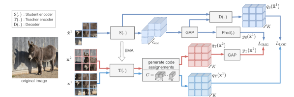
Figure 2: Overview of MOCA. The teacher (bottom) takes as an input two unmasked random views $\mathbf{x}^{\{1,2\}}$ of the same image and generates dense token-wise code assignments $q_{\mathrm{T}}(\mathbf{x})$ for them (i.e., soft-assigns codebook items to the patch tokens). The student (top) receives as an input a randomly masked image version $\tilde{\mathbf{x}}^{1}$ of view $\mathbf{x}^{1}$ and is trained to minimize two types of self-supervised losses: (1) A masked same-view token assignment prediction loss $L_{\text{LOC}}$, which requires predicting the teacher-produced assignment vectors of view $\mathbf{x}^{1}$ from the corresponding masked image $\tilde{\mathbf{x}}^{1}$. This is a spatially dense loss that enables learning representations with dense contextual reasoning. (2) A masked cross-view average assignment prediction loss $L_{\text{IMG}}$, which is to predict with the global image embedding of the first view $\tilde{\mathbf{x}}^{1}$ the average assignment vector of the opposite view $\mathbf{x}^{2}$ (‘GAP’ stands for Global Average Pooling). This is an image-wise loss that promotes learning image representations that are invariant with respect to different augmentations of the input. The same objectives are applied in a symmetric way when the student gets as input the masked image version $\tilde{\mathbf{x}}^{2}$ of view $\mathbf{x}^{2}$ (not shown). We implement the $L_{\text{LOC}}$ objective with a condenser-based decoder that gets as input patch-token embeddings from an intermediate layer of the student encoder and the global image embeddings from its last layer (see Sec. 3.3). The teacher is an exponential moving average (‘EMA’) of student.

Our goal is to build a hide-and-predict self-supervised approach that (a) is defined over high-level concepts and (b) is standalone (i.e., does not require any pre-trained model or off-line training stage). To this end, we follow a teacher-student setup where the teacher transformer $\mathrm{T}(\cdot)$ is a momentum-updated version [38, 65] of the student transformer $\mathrm{S}(\cdot)$ and generates targets for its student (Figure 2).

For defining these targets, we use what we will refer to hereafter as token assignment vectors (over an online codebook), which constitute the high-level visual concepts over which our hide-and-predict framework is defined. We detail the definition of these assignment vectors in Sec. 3.1. We then describe in Sec. 3.2 how we use these teacher-produced assignment vectors for defining the hide-and-predict objectives for the student transformer training. In Sec. 3.3 we discuss important design choices, in Sec. 3.4 techniques for faster training and in Sec. 3.5 implementation details.

3.1 Teacher-produced token assignment vectors

Given as input an image token sequence $\mathbf{x}=\{\mathbf{x}_{i}\}_{i=1}^{N}$, the teacher encoder transformer first extracts $d_{\text{enc}}$-dimensional token embeddings $\mathrm{T}(\mathbf{x})=\{\mathrm{T}(\mathbf{x})_{i}\}_{i=1}^{N}$, and then soft-quantizes them over a codebook $C=[\mathbf{c}_{1},\ldots,\mathbf{c}_{K}]$ of $K$ embeddings of dimension $d_{\text{enc}}$. This produces the soft-assignment vectors $q_{\mathrm{T}}(\mathbf{x})=\{q_{\mathrm{T}}(\mathbf{x})_{i}\}_{i=1}^{N}$, where $q_{\mathrm{T}}(\mathbf{x})_{i}$ is a $K$-dimensional vector computed as the cosine similarity of the token embedding $\mathrm{T}(\mathbf{x})_{i}$ and each codebook embedding $\mathbf{c}_{k}$, followed by a softmax with temperature $\tau_{T}$ (which controls the softness of the assignment). In essence, $q_{\mathrm{T}}(\mathbf{x})_{i}$ encodes the assignment of $\mathrm{T}(\mathbf{x})_{i}$ to its closest (in terms of cosine distance) codebook embeddings. We use these teacher-produced assignment vectors for defining the hide-and-predict objectives for the student transformer training, which is described in Sec. 3.2.

The embeddings in codebook $C$ are teacher-token embeddings that were randomly sampled from previous mini-batches. In particular, at each training step, after computing the assignment vectors, we randomly sample $K_{\text{new}}\ll K$ token embeddings from the current mini-batch, each from a different image. Therefore, we always keep the sampled embeddings from only the past $K/K_{\text{new}}$ mini-batches in the memory (which is implemented as a queue).

3.2 Hide-and-predict token assignment vectors

Let $\mathbf{x}^{v}$ with $v\!\in\!\{1,\,2\}$ be the token sequences of two random views sampled from the same training image. On the teacher side, they are processed by the transformer $\mathrm{T}(\cdot)$ to produce a sequence of image token assignment vectors $q_{\mathrm{T}}(\mathbf{x}^{v})$. On the student side, the transformer $\mathrm{S}(\cdot)$ receives as input randomly masked versions of the $\mathbf{x}^{v}$ images, which are denoted by $\tilde{\mathbf{x}}^{v}$ with $v\in\{1,2\}$, and is trained to minimise two types of masked-based self-supervised losses:

1. A masked same-view token assignment prediction loss $L_{\mathrm{LOC}}$, which aims at predicting the sequence of teacher assignment vectors $q_{\mathrm{T}}(\mathbf{x}^{v})$ from the corresponding masked image $\tilde{\mathbf{x}}^{v}$ for $v\in\{1,2\}$. This is a spatially dense loss whose role is to enable learning representations with dense contextual reasoning skills.

2. A masked cross-view average assignment prediction loss $L_{\mathrm{IMG}}$, which amounts to predicting the teacher’s average assignment vector of the first view, $y_{\mathrm{T}}(\mathbf{x}^{1})$, from the opposite masked view $\tilde{\mathbf{x}}^{2}$ and vice-versa. This is an image-wise loss whose role is to promote learning image representations that are invariant with respect to different augmentations of the input.

The overall training loss for the student model is:

$$L=\lambda L_{\mathrm{IMG}}+(1-\lambda)L_{\mathrm{LOC}},$$ (1)

where $\lambda\in[0,1]$. Unless stated otherwise, we use $\lambda=0.5$. In the following, we describe these two objectives in detail.

Masked same-view token assignment prediction.  With this objective, given as input the masked view $\tilde{\mathbf{x}}^{v}$, the student is trained to predict the assignment vectors of the tokens as generated by the teacher from $\mathbf{x}^{v}$. In the following, for each $v\in\{1,2\}$, we denote by $u_{v}\subset\{1,...,N\}$ the set of indices of all tokens that remain unmasked (i.e., all tokens from view $\mathbf{x}^{v}$ that are seen by the student) and by $m_{v}\subset\{1,...,N\}$ the set of indices of all the masked tokens (it holds $m_{v}\cup u_{v}=\{1,...,N\}$ and $m_{v}\cap u_{v}=\emptyset$).

For computational efficiency reasons, the student encoder $S(\cdot)$ processes only the unmasked tokens. Therefore, for the prediction of the masked token assignment vectors of the teacher, we employ on the student side an additional decoder transformer $\mathrm{D}(\cdot)$. For this prediction to take place, in the default setup, we employ the following steps:

Encoding the masked view:

We first give the unmasked tokens $\tilde{\mathbf{x}}^{v}=\{\mathbf{x}^{v}_{i}\}_{i\in u_{v}}$ as input to the student encoder transformer $\mathrm{S}(\cdot)$ to produce the $d_{\text{enc}}$-dimensional student token embeddings $\{\mathrm{S}(\tilde{\mathbf{x}}^{v})_{i}\}_{i\in u_{v}}$.

Decoder input embedding:

Before we give the encoder embeddings as input to the decoder, we apply to them a linear projection layer to convert their dimensionality from $d_{\text{enc}}$ to $d_{\text{dec}}$, where $d_{\text{dec}}$ is the dimensionality of the decoder embeddings. Then, we append the encoder embeddings with a learnable masked embedding for each masked token $i\in m_{v}$ and add (non-learnable sin-cos-based) positional embeddings to them. We denote the set of embeddings produced from this step as $\mathbf{z}^{v}$.

Local token assignment prediction:

Last, the above embeddings are given as input to the decoder transformer $\mathrm{D}(\cdot)$. The decoder computes the tokens embeddings $\mathrm{D}(\mathbf{z}^{v})=\{\mathrm{D}(\mathbf{z}^{v})_{i}\}_{i=1}^{N}$, which will be used for predicting the token assignment vectors as follows:

$$q_{\mathrm{S}}(\tilde{\mathbf{x}}^{v})_{i}=\operatorname{softmax}(\frac{1}{\tau_{d}}\,\mathrm{D}(\mathbf{z}^{v})_{i}^{\top}W^{d}),$$ (2)

for $i\in\{1,...,N\}$. The weights $W^{d}=[\mathbf{w}^{d}_{1},\cdots,\mathbf{w}^{d}_{K}]$ are $L_{2}$-normalized $d_{\text{dec}}$-dimensional prototypes (one per codebook embedding in $C$) used for predicting the assignment vectors. As we will explain in more detail later on (see Sec. 3.5), these prototypes are not learnt but are dynamically generated by a weight generation module. Also, $\tau_{d}$ is a softmax temperature that controls the softness of the predicted probability.

The masked same-view token assignment prediction loss is

$$L_{\mathrm{LOC}} =L^{1}_{\mathrm{LOC}}+L^{2}_{\mathrm{LOC}},\text{ where}$$ (3)

$$L^{v}_{\mathrm{LOC}} =\sum_{i}\mathrm{CE}\big{(}q_{\mathrm{S}}(\tilde{\mathbf{x}}^{v})_{i},q_{\mathrm{T}}(\mathbf{x}^{v})_{i}\big{)},\,\forall v\in\{1,2\},$$ (4)

and $\mathrm{CE}(\mathbf{a},\mathbf{b})\!=\!-\!\sum_{k=1}^{K}\mathbf{b}[k]\log(\mathbf{a}[k]\big{)}$ is the cross-entropy loss between two distributions $\mathbf{a}$ and $\mathbf{b}$.

Masked cross-view average assignment prediction.  In this objective, we first reduce the teacher assignments $q_{\mathrm{T}}(\mathbf{x})\!=\!\{q_{\mathrm{T}}(\mathbf{x})_{i}\}_{i=1}^{N}$ to a single $K$-dimensional vector $y_{\mathrm{T}}(\mathbf{x})$ via global average pooling, i.e., we reduce $q_{\mathrm{T}}(\mathbf{x})$ to a ‘bag-of-word’ (BoW) representation. Then, similar to BoW-prediction methods [34, 33], for each view $v$ the student must predict with its global image embedding $\bar{\mathrm{S}}(\tilde{\mathbf{x}}^{v})$ the reduced assignment vector of the opposite view as follows:

$$y_{\mathrm{S}}(\tilde{\mathbf{x}}^{v})=\operatorname{softmax}(\frac{1}{\tau_{b}}\,\bar{\mathrm{S}}(\tilde{\mathbf{x}}^{v})^{\top}W^{b}).$$ (5)

As in the same-view token assignment prediction, $\tau_{b}$ is the softmax temperature, and $W^{b}=[\mathbf{w}^{b}_{1},\cdots,\mathbf{w}^{b}_{K}]$ are $L_{2}$-normalized $d_{\text{enc}}$-dimensional prototypes that are dynamically generated by a weight generation module.

The cross-view image-wise training loss that is minimized for the two masked image views $\tilde{\mathbf{x}}^{v}$ with $v\in\{1,2\}$, is

$$L_{\mathrm{IMG}}\!=\!\mathrm{CE}\big{(}y_{\mathrm{S}}(\tilde{\mathbf{x}}^{1}),y_{\mathrm{T}}(\mathbf{x}^{2})\big{)}\!+\!\mathrm{CE}\big{(}y_{\mathrm{S}}(\tilde{\mathbf{x}}^{2}),y_{\mathrm{T}}(\mathbf{x}^{1})\big{)}.\!$$ (6)

3.3 Learning high-level target assignment vectors

To make our hide-and-predict approach effective, it is crucial for the teacher to learn assignment vectors that encode high-level/semantic visual concepts. In the context of our teacher-student scheme, where the teacher is a slower-moving version of the student, this depends on the student first learning patch-token embeddings (from where the assignment vectors are extracted at the teacher side) that capture this type of visual features. Below we detail the critical role some design choices have in that.

Condenser-based decoding.  As in [31, 60], we change the default setup described in Sec. 3.2 and create a bottleneck in the decoding task that promotes the student’s global image representation to capture more spatial structure from the input view $\tilde{\mathbf{x}}$. The bottleneck is introduced by changing the way the decoder input embeddings $\mathbf{z}^{v}$ are formed.

In particular, instead of using as input to the decoder the token patch embeddings $\{\mathrm{S}(\tilde{\mathbf{x}}^{v})_{i}\}_{i\in u_{v}}$ (coming from its last layer), we give as input (a) token embeddings $\{\mathrm{S}^{\ell}(\tilde{\mathbf{x}}^{v})_{i}\}_{i\in u_{v}}$ from an intermediate transformer layer $\ell$ of $\mathrm{S}$ together with (b) the last layer’s global image embedding $\bar{\mathrm{S}}(\tilde{\mathbf{x}}^{v})$. Using lower-layer embeddings for the patch tokens enforces the global image embedding $\bar{\mathrm{S}}(\tilde{\mathbf{x}}^{v})$ (which is used as global image representation for downstream tasks like k-NN and linear probing) to capture more information so as to compensate for the added decoding bottleneck.

Hide-and-predict using the [AVG] token.  The average patch embedding $\bar{\mathrm{S}}(\tilde{\mathbf{x}}^{v})=\frac{1}{|u_{v}|}\sum_{i\in u_{v}}\mathrm{S}(\tilde{\mathbf{x}}^{v})_{i}$ (called [AVG] token for brevity) is used for performing (a) the cross-view image-wise prediction task (see Eq. 5), which is crucial for promoting perturbation invariances, as well as (b) the condenser-based decoding that was explained above. Therefore, using the [AVG] token (instead of the [CLS] token) results in the student’s patch embeddings $\{\mathrm{S}(\tilde{\mathbf{x}}^{v})_{i}\}_{i\in u_{v}}$ (from which the [AVG] token is computed) to receive a more direct supervisory signal from the two prediction losses. Consequently, these embeddings (i) are steered to encode the perturbation-invariant and context/structure-aware information necessary for performing the two prediction objectives, and (ii) are typically of a more semantic nature.

The impact of these design choices is studied in Sec. 4.1.

3.4 Masking strategies for efficient training

Decoder depth	2	4	8
Time (min)	9.00 $\rightarrow$ 8.15	10.25 $\rightarrow$ 8.55	12.41 $\rightarrow$ 9.30
Memory (GB)	30.4 $\rightarrow$ 23.0	37.7 $\rightarrow$ 26.2	52.4 $\rightarrow$ 32.6

Table 1: Time & memory savings of partial decoding. We report training time (per epoch) and GPU memory savings for ViT-B/16 when switching from full to partial decoding, measured under 8-A100 GPU node and total batch size $2048$.

Objectives	$L_{\mathrm{IMG}}$	$L_{\mathrm{IMG}}$ & $L_{\mathrm{LOC}}$
	($\lambda=1.0$)	($\lambda=0.5$)
Condenser	N/A	✗	baselinecolor✓
k-NN	66.8	67.8	baselinecolor71.8

(a)

Depth	1	baselinecolor2	4	8
k-NN	71.7	baselinecolor71.8	70.9	70.5
Time (min)	8.08	baselinecolor8.15	8.55	9.3
Memory (GB)	21.5	baselinecolor23.0	26.2	32.6

(b)

Mask ratio	55%	baselinecolor65%	75%	80%
k-NN	72.6	baselinecolor71.8	69.8	68.4
Time (min)	9.00	baselinecolor8.15	7.37	7.35
Memory (GB)	28.6	baselinecolor23.0	18.2	15.7

(c)

	[CLS]	baselinecolor[AVG]
k-NN	60.2	baselinecolor71.8

(d)

$\lambda$	1.0	0.75	baselinecolor0.5	0.25	0.00
k-NN	66.8	70.2	baselinecolor71.8	71.5	13.1

(e)

Layer $\ell$	6	baselinecolor8	9	10
k-NN	71.4	baselinecolor71.8	71.5	70.9

(f)

Table 2: MOCA ablation. k-NN classification on ImageNet-1k with a ViT-B/16 trained for 100 pre-training epochs and 1 masking round. Default setting (in gray): $\lambda=0.5$, mask ratio of $65\%$, [AVG] token used as global image embedding, condenser-based decoder with depth 2 fed with patch-embeddings from the $\ell=8$ intermediate student layer.

Partial decoding for efficient training.  We randomly select the token indices $m_{v}$ to be masked from each view, with a relatively high percentage of masked tokens (i.e., $65\%$). This results in significant computational and GPU memory savings from the student encoder side during training. However, some of these savings are lost if the decoder processes all masked tokens. To mitigate this, we propose inputting only a small subset $m^{\prime}_{v}\subset m_{v}$ of masked tokens, along with the visible tokens, to the decoder. For example, instead of inputting all $65\%$ of image tokens that we mask from the student, we input only a random subset, e.g., $20\%$ of the total image tokens. As shown in Tab. 1, this results in noticeable savings in computation and GPU memory, especially for many-layer decoders, without any loss in the quality of learned representations (as we demonstrate in Sec. 4.1). Note that although we only tested partial decoding in the context of our approach, we believe it could benefit other hide-and-predict methods as well, e.g., MAE [37].

Faster training convergence with 2nd masking round.  With our partial decoding, we can allocate our computation budget to enhance the model’s performance with other techniques. Specifically, we apply a second round of random token masking to both views and then perform the assignment prediction objectives with the newly generated masked views in the same manner as before. This technique artificially increases the batch size and saves time since we can reuse the teacher assignment vectors from the first masking round. It can be seen as a form of batch augmentation [40, 71] that reduces gradient variance by having in the same mini-batch multiple randomly augmented copies of the same sample.

3.5 Implementation details

Dynamic prototype generation modules.  Our method updates the codebook $C$ at the teacher side at each training iteration with new randomly-sampled teacher-token embeddings. Due to this, instead of learning the prototypes $W^{d}$ and $W^{b}$ that are used on the student side for the two assignment prediction tasks defined by Eqs. 2 and 5, we dynamically generate them using two weight generation modules. In particular, we employ the generation networks $\mathrm{G}^{b}(\cdot)$ and $\mathrm{G}^{d}(\cdot)$ that at each training step take as input the current codebook $C=[\mathbf{c}_{1},\ldots,\mathbf{c}_{K}]$ and produce for them the prototypes weights $W^{b}=\mathrm{G}^{b}(C)=[\mathrm{G}^{b}(\mathbf{c}_{1}),\dots,\mathrm{G}^{b}(\mathbf{c}_{K})]$ and $W^{d}=\mathrm{G}^{d}(C)=[\mathrm{G}^{d}(\mathbf{c}_{1}),\dots,\mathrm{G}^{d}(\mathbf{c}_{K})]$ respectively. The generation networks $\mathrm{G}^{b}(\cdot)$ and $\mathrm{G}^{d}(\cdot)$ are implemented with 2-layer perceptrons (i.e., each as a sequence of Linear, BN, ReLU, and Linear layers), whose input and output vectors are $L_{2}$-normalized.

Model hyper-parameters.  We use $\tau_{b}=\tau_{d}=\frac{1}{3}$ for the softmax temperatures at the student side; and $\tau_{T}=\frac{1}{10\cdot\bar{\mu}_{\text{MSD}}}$ at the teacher’s side, where $\bar{\mu}_{\text{MSD}}$ is the exponential moving average (with momentum $0.99$) of per-image token difference between the maximum cosine similarity over the codebook embeddings and the average cosine similarity. For the codebook, we use $K=4096$.

4 Experiments

Setup.  In this section, we evaluate our MOCA method by training ViT-B/16 models on the ImageNet-1k [66] dataset. We use the AdamW optimizer [52] with $\beta_{1}=0.9$, $\beta_{2}=0.999$ and weight decay $0.05$. The batch size is $2048$ split over 8 A100 GPUs. For the learning rate $lr$, we use a linear warm-up from $0$ to its peak value for $30$ epochs and then we decrease it over the remaining epochs with a cosine annealing schedule. We use a peak $lr$ value of $1.5\times 10^{-4}$ and train the models for $100$ or $200$ epochs. More implementation details are provided in the supplementary material.

4.1 Method analysis

We first study several aspects of our approach with ablative experiments, in which we train ViT-B/16 models for $100$ epochs. Except stated otherwise, the models include the condenser-based decoder (Sec. 3.3), partial decoding, and a single token masking round. We evaluate the learned representations on the k-NN ImageNet classification task.

Integrating the two masked prediction objectives.  Here we show that a naive integration of the two masked-prediction objectives does not work effectively.

Ablating the condenser-based decoding in LABEL:tab:condenser_ablation.  Compared to a model trained only with the image-wise objective $L_{\mathrm{IMG}}$, a naive implementation of our dense hide-and-predict objective $L_{\mathrm{LOC}}$ without the condenser design principle provides only a small k-NN performance improvement (i.e., $+1$ point). Instead, when using the condenser, the k-NN performance increase is much larger (i.e., $+5$ points). We further compare the performance with and without condenser and 200 pre-training epochs (instead of 100) in Tab. 4: condenser leads to significantly better results in all evaluation protocols, apart from ImageNet fine-tuning. On the other hand, in this longer pre-training setting the naive implementation of $L_{\mathrm{LOC}}$ achieves worse results than only using $L_{\mathrm{IMG}}$ in k-NN and linear probing. These results validate that the condenser design choice indeed leads to a more effective hide-and-predict training (see discussion in Sec. 3.3). In LABEL:tab:impact_of_intermediate_layer we see that using $\ell=8$ as the intermediate student layer for providing the patch-token embeddings that are given as input to the condenser-based decoder, gives the best results.

Partial Dec.	#Masks	k-NN	Time (min)	Memory (GB)
✗	1	71.6	$9.00$	30.4
✓	1	71.8	$8.15$	23.0
✓	2	74.4	$10.35$	39.5

Table 3: Training efficiency ablations. k-NN classification results on ImageNet-1k with ViT-Base-16 models pre-trained for 100 epochs. #Masks is the number of different masks per view. #Partial is doing partial token decoder. Time is the per epoch training time and Memory is the GPU footprint, both measured with single 8-A100 node and batch size $2048$.

[CLS] vs. [AVG] global embedding tokens (LABEL:tab:csl_vs_avg). Using the [CLS] token as the global embedding, instead of the average embedding token ([AVG]), significantly decreases the k-NN performance (i.e., $-11.6$ points). This is because, as discussed in Sec. 3.3, the [AVG] token leads to learning assignment vectors that encode more high-level concepts and thus makes our hide-and-predict method more effective.

Balancing the two prediction objectives.  The $\lambda$ hyperparameter controls the importance of the two assignment prediction objectives (see Eq. 1). We see in LABEL:tab:impact_lambda that $\lambda=0.5$ gives the best results while switching off any of the two objectives ($\lambda=1$ or $\lambda=0$) seriously deteriorates the k-NN performance. This suggests that the objectives work in a complementary and synergistic way. For instance, for $\lambda=0$ (no $L_{\mathrm{IMG}}$ loss) the results are very poor. The reason is that without the image-wise loss, it is hard to bootstrap the learning of teacher-produced assignment vectors that encode high-level concepts (see discussion in Sec. 3.3). In the supplementary, we report more experiments, results, and discussions about the behavior when training without the image-wise loss $L_{\mathrm{IMG}}$.

Decoding and masking strategies.

Studying the impact of decoder depth in LABEL:tab:impact_dec_depth. We observe that our method behaves better with “shallower” decoders, in contrast to what is the case in MAE (which uses a decoder with eight layers). This is expected since our hide-and-predict objectives require the decoder to predict high-level concepts. In that case, it is better for the applied loss to be “closer” to the student (i.e., having a shallower decoder) so as to promote the output student embeddings to capture such high-level information in a more “ready-to-use” way. On the other hand, MAE’s decoder, which must reconstruct pixels, is better to be deeper and thus spare the MAE’s encoder from capturing such low-level details. Furthermore, using a “shallower” decoder leads to significant computation and GPU memory savings in our case.

Partial decoder and 2nd masking round in Tab. 3. Switching off partial decoding (i.e., decoding all the masked tokens) leads to an increase in the per-epoch training time and GPU memory usage with zero benefits on the quality of the learned features as measured with k-NN. Instead, having a second round of token masking, although increasing the training time and GPU memory usage, leads to a significant k-NN performance boost. Therefore, we employ it for the final model that we train for the results in Sec. 4.3.

Studying the masking ratio impact in LABEL:tab:mask_ratio. The 55% and 65% ratios give the best results.

4.2 Comparison of hide-and-predict objectives.

In our work, we propose a hide-and-predict objective $L_{\mathrm{LOC}}$ that is defined in the space of assignment vectors over an online-updated codebook. In Tab. 4, we compare this objective (‘Assign.’) against (a) a hide-and-predict objective defined in the pixel space with per-patch normalization as in MAE [37] (‘Pixels’); and (b) a hide-predict-objective in which the decoder must directly regress the $c_{\text{enc}}$-dimensional output teacher-token embeddings (before any code assignment) using a cosine-distance loss (‘Embeddings’). We keep the image-wise $L_{\mathrm{IMG}}$ objective intact for all three models. The Embeddings model is implemented with a condenser-based decoder of depth two, as with our Assignments model, while the Pixels model uses a standard decoder and depth four (which gives better results). All other model hyper-parameters remain the same for fair comparison. We see that the Assignments model produces superior results on all three ImageNet classification evaluation protocols. This demonstrates the advantage of defining a hide-and-predict objective with online codebook assignment vectors as targets.

Objectives	$L_{\mathrm{IMG}}$	$+$hide-and-predict variants
Targets		Assign.	Assign. (ours)	Pixels	Embeddings
Condenser	N/A	✗	✓	✗	✓
k-NN	72.0	70.0	75.4	72.3	73.6
Linear	76.1	75.7	77.7	76.4	76.9
Fine-tune	82.7	83.5	83.4	83.2	83.0

Table 4: Ablating hide-and-predict variants. ImageNet-1k classification results with ViT-B/16 models pre-trained for 200 pre-training epochs with a single token masking round.

Method	#Epoch	Linear	Finetuning
CIM [29]	300	-	83.1
CAE [16]	800	68.6	83.8
CAE [16]	1600	70.4	83.9
BEiT [6]	800	37.6	83.2
SimMIM [78]	800	56.7	83.8
MAE [37]	800	68.0	83.1
MAE [37]	1600	68.0	83.6
CAN [54]	800	74.0	83.4
CAN [54]	800	74.8	83.6
MOCA (ours)	200	78.7	83.6

Table 5: Comparison with hide-and-predict methods. ImageNet classification results with ViT-B/16.

4.3 Comparative results

We compare our method against other hide-and-predict methods as well as self-supervised methods based on teacher-student or contrastive objectives. To this end, we train a ViT-B/16 model for $200$ epochs with a condenser-based decoder, two masking rounds (the 1st with 55% mask ratio and the 2nd with 75% mask ratio), and partial decoding only 20% of patch tokens per masking round.

Full and low-shot image classification.  We first evaluate the learned representations on ImageNet classification with the k-NN, linear probing, and fine-tuning evaluation protocols and using the full training set. Moreover, we evaluate low-shot ImageNet classification with logistic regression [3].

Comparison with hide-and-predict approaches. In Tab. 5, we compare our method MOCA against other self-supervised methods with MIM objectives. We observe that on linear probing MOCA achieves superior performance to all the other works, with more than 2 points. This demonstrates that MOCA is better at learning “ready-to-use” features. At the same time, its fine-tuning performance is on par with the state-of-the-art, falling only 0.3 points behind the top-performing method. This is despite MOCA using only 200 epochs and a smaller computational budget in general. For instance, as we can see in Tab. 7, the total training time of our method is more than 3.5 times smaller compared to MAE, which is (one of) the most training-efficient methods.

Comparison with teacher-student and contrastive methods. In Tab. 6, we compare our method against other self-supervised methods based on contrastive objectives or teacher-student schemes. We observe that our method is superior to competing approaches that do not use multiple crops and is on par with them when they employ such techniques. Again, we emphasize that our method is much more computationally efficient than these techniques (see Tab. 7).

Method	#Epoch	k-NN	Linear	Finetuning
MoCo-v3 [19]	300	-	76.7	83.0
DINO [14]	400	68.9	72.8	-
iBOT [88]	400	71.2	76.0	-
DINO$\dagger$ [14]	400	76.1	78.2	82.8
iBOT$\dagger$ [88]	400	77.1	79.6	84.0
MSN$\dagger$ [3]	600	-	-	83.4
MOCA (ours)	200	77.2	78.7	83.6

Table 6: Comparison with teacher-student and contrastive methods. ImageNet classification results with ViT-B/16. $\dagger$: use of multiple crops[14].

Method	#Epoch	Time / epoch	Total time
MAE [37]	1600	5.35 min	142 hours
DINO [14]	400	16.42 min	109 hours
iBOT [88]	400	17.40 min	116 hours
DINO$\dagger$ [14]	400	23.16 min	154 hours
iBOT$\dagger$ [88]	400	24.33 min	162 hours
MOCA (ours)	200	11.23 min	38 hours

Table 7: Training time comparisons with ViT-B/16 as encoder. The per-epoch time measurements are based on a single 8 A100 GPU node. $\dagger$: use of multiple crops[14].

		#Images per class
Method	#Epoch	1	2	5	$\approx$13
MAE [37]	1600	$\,\,\,8.2\pm 0.3$	$25.0\pm 0.3$	$40.5\pm 0.2$	$51.1$
DINO$\dagger$ [14]	400	$41.8\pm 0.3$	$51.9\pm 0.6$	$61.4\pm 0.2$	$67.2$
iBOT$\dagger$ [88]	400	$46.1\pm 0.3$	$56.2\pm 0.7$	$64.7\pm 0.3$	$69.7$
MSN$\dagger$ [3]	600	$49.8\pm 0.2$	$58.9\pm 0.4$	$65.5\pm 0.3$	$69.4$
MOCA (ours)	200	$\textbf{55.4}\pm 0.4$	$\textbf{63.9}\pm 0.2$	$\textbf{69.9}\pm 0.1$	72.4

Table 8: Low-shot evaluation on ImageNet-1k. Top-1 accuracy results with ViT-B/16. $\dagger$: use of multiple crops[14].

Low-shot classification. Here, for ImageNet-1k classification, we adopt the low-shot evaluation protocol of MSN [3] and use as few as 1, 2, or 5 training images per class as well as using $1\%$ of the ImageNet-1k’s training data, which corresponds to $\approx$13 images per class. In particular, for this low-shot training setting, we extract global image embeddings with the pre-trained transformer (average patch embeddings computed by the teacher) and train a linear classifier on top of it with the few available training data. As we see from the results in Tab. 8 (see also Fig. 1), MOCA outperforms prior methods with ViT-B/16 – surpassing the second best method MSN [3] by a large margin.

Full and low-shot semantic segmentation.  We further evaluate our method on the Cityscapes [21] semantic segmentation dataset, by either linear probing or finetuning. We use the Segmenter [67] model with ViT-B/16 backbone initialized either with our MOCA or other self-supervised methods. For linear probing, we append a linear layer to the frozen encoder and train the models either with the complete $2975$-image Cityscapes training set or in the few-shot setup with 3 different splits of $100$ images each [30]. For finetuning, we use a single mask transformer layer as a decoder following the original setup [67] and train on the full training set.

In Tab. 9, we show the best results on the $500$ validation images. Learning rates were optimized for every method separately, with other hyperparameters kept as the default ones used in the Segmenter [67] codebase. The results show the superiority of MOCA in all the setups. In the linear probing experiments, the results demonstrate that MOCA provides better high-level “ready-to-use” image representations compared to the other methods, outperforming the closest competitor iBOT [88] by up to $0.8$/$2.1$ mIoU in the full/few-shot scenarios. As expected, MAE [37] struggles in these setups. MOCA achieves the best results also in the fine-tuning setup, although the gap between the methods is shrunk there.

Setup	MAE [37]	DINO$\dagger$ [14]	iBOT$\dagger$ [88]	MOCA (ours)
Linear (Full)	40.6	55.5	59.3	60.1
Linear (FS)	33.2	45.8	47.8	49.9
Finetuning (Full)	77.7	75.7	77.8	78.2

Table 9: Semantic segmentation on Cityscapes [21]. We report mIoU results using a Segmenter [67] model with ViT-B/16 backbone. ‘Full’: using all the $2975$ training images. ‘FS’: using three different splits of $100$ training images each (we average the results over the three splits).

5 Conclusion

In this work we have proposed a novel self-supervised learning framework that is able to exhibit the complementary advantages of both discriminative and hide-and-predict approaches, thus promoting visual representations that are perturbation invariant, encode semantically meaningful features and also exhibit dense contextual reasoning skills. To that end, we make use of a novel masking-based strategy that operates in the space of high-level assignment vectors that are produced in an online and standalone fashion (i.e., without the need for any pre-trained models or multiple training stages) using a teacher-student scheme and an online generated codebook. We have experimentally shown that our approach possesses significant computational advantages compared to prior methods, while exhibiting very strong performance, not only in the case of full finetuning but also in the case of linear probing and k-NN classification settings. It thus allows us to obtain high-quality image representations with much smaller training computational budget compared to prior state-of-the-art approaches.

Acknowledgements.

This work was performed using HPC resources from GENCI-IDRIS (Grants 2022-AD011012884R1 and 2022-AD011013413), from CINES under the allocation GDA2213 for the Grand Challenges AdAstra GPU made by GENCI, and Youth and Sports of the Czech Republic through the e-INFRA CZ (ID:90140), by CTU Student Grant SGS21184OHK33T37. This research received the support of EXA4MIND, a European Union’s Horizon Europe Research and Innovation program under grant agreement N° 101092944. Views and opinions expressed are however those of the authors only and do not necessarily reflect those of the European Union or the European Commission. Neither the European Union nor the granting authority can be held responsible for them.

Appendix A Additional experimental results

A.1 Cityscapes semantic segmentation

Setup	#train	MAE[37]	DINO$\dagger$[14]	iBOT$\dagger$[88]	MOCA (ours)
Linear	2975	40.6	55.5	59.3	60.1
Linear	372	39.6	51.0	54.0	55.2
Linear	100	33.2	45.8	47.8	49.9
Fine-tuning	2975	77.7	75.7	77.8	78.2
Fine-tuning	372	62.6	65.7	66.8	71.1
Fine-tuning	100	41.4	47.7	48.6	51.5

(c) Detailed results with both linear probing and fine-tuning.

Figure 3: Semantic segmentation on Cityscapes. We visualize (a)-(b) and report (c) mIoU results using a Segmenter [67] model with ViT-B/16 backbone. For training we use $100$, $372$ or $2975$ (full) images from the Cityscapes training set using random splits from [30]. $\dagger$: use of multi-crop augmentation during pre-training [14].

Here we evaluate MOCA on the Cityscapes [21] semantic segmentation dataset, by either linear probing or fine-tuning, using more low-shot settings. In particular, in Fig. 3, we report mIoU semantic segmentation results with both linear probing and full fine-tuning using $100$ or $374$ training images, representing $1/30$ and $1/8$ of the full Cityscapes training set of $2975$ images. We include the evaluation on the full training set as well. For the $100$ and $374$ low-shot settings, we use three different splits of $100$ or $374$ training images respectively following the protocol from[30] and report the average mIoU performance over the three splits.

We report the linear probing results in Fig. 3(a) and fine-tuning results in Fig. 3(b) and provide detailed results in the table (c). They show that our method achieves consistently superior performance to prior methods.

A.2 Training without the $L_{\mathrm{IMG}}$ objective

	Decoder approach
	Default	Condenser	Targets	k-NN	Linear
(a)	✓		Assign.	34.4	51.6
(b)		✓	Assign.	13.1	33.7
(c)	✓	✓	Assign.	52.5	64.2
(d)	✓		Pixels	14.6	38.8
(e)		✓	Pixels	15.6	42.7
(f)	✓	✓	Pixels	13.9	41.9

Table 10: Hide-and-predict models trained without the $L_{\mathrm{IMG}}$ loss ($\lambda=0$). ImageNet-1k classification results with ViT-B/16 models trained for 100 pre-training epochs with a single token masking round. For these models, we use the default and/or the condenser decoder versions.

In Tab. 10, we report more results from MOCA trainings with only the $L_{\mathrm{LOC}}$ loss and the $L_{\mathrm{IMG}}$ loss deactivated (i.e., setting $\lambda=0$). The decoder of these models is implemented using: (a) the default approach described in Sec. 3.2, or (b) the condenser-based approach described in Sec. 3.3. We also provide results for when having two decoders (c), one using the default approach and the other the condenser-based approach, each trained with a separate $L_{\mathrm{LOC}}$ loss.

We observe that, with only the $L_{\mathrm{LOC}}$ loss, the default decoder (model (a)) is better than the condenser-based decoder (model (b)), which is the opposite from the behavior when both the $L_{\mathrm{LOC}}$ and the $L_{\mathrm{IMG}}$ objectives are used. The fact that the optimal choice for the decoder is different depending on whether $L_{\mathrm{IMG}}$ is used or not shows that the two objectives work together in a synergistic way. Nevertheless, even with the default decoder (model (a)) the k-NN and Linear probing performances are still quite low. However, model (c), which combines the two decoders, fares much better. Indeed, in this case, the model better bootstraps its learning process and, thus, learns better image representations.

We also compare with variants where the hide-and-predict objectives are defined in the pixel space with per-patch normalization as in MAE [37] (‘Pixels’). We see that in this pixel-reconstruction case, the decoder type has a small impact. Also, our assignment-prediction models (a) and (c) achieve significantly better k-NN and Linear probing performance than these pixel-reconstruction models, which shows the interest in exploiting higher-level features.

A.3 Longer pre-training

Method	#Epoch	k-NN	Linear	Finetun.	1-shot	2-shot	5-shot
MOCA ViT-B/16	200	77.2	78.7	83.6	55.4	63.9	69.9
MOCA ViT-B/16	400	77.6	79.3	83.7	55.5	64.6	69.9
MOCA ViT-L/16	200	78.4	80.3	84.9	56.3	65.2	70.7

Table 11: Scaling pre-training epochs or model size. Top-1 accuracy results on ImageNet with ViT-B/16 or ViT-L/16.

Method	#Epoch	Time	k-NN	Linear	Finetun.
MAE	1600	187h	-	75.1	85.9
iBOT$\dagger$	300	320h	78.0	81.0	84.8
MOCA	200	89h	78.4	80.3	84.9

Table 12: ViT-L/16 comparisons. Top-1 accuracy results on ImageNet. The time measurements are based on a single 8 A100 GPU node. $\dagger$: use of multiple crops[14].

As we see in Table 11, longer pre-training in MOCA improves performance, but with diminishing returns. This behavior is similar to other pre-training methods, where performance converges after a certain number of pre-training epochs. MOCA’s advantage lies in its faster convergence, effectively reducing pre-training time.

A.4 Bigger backbones

As we see in Tables 11 and 12, MOCA can scale with bigger backbones and achieves strong results while it has smaller pre-training time.

A.5 COCO detection and instance segmentation results

We present supplementary results on COCO detection and instance segmentation in Table 13. MOCA demonstrates strong performance in these tasks. We use the COCO 2017 set consisting of $118$K training images, $5$k validation and $20$ test-dev. For this experiment we follow the implementation from [49]. In detail, we adopt Cascade Mask R-CNN [39, 9] as task layer and use a similar hyper-paramenter configuration for ViT-B with  [88]: multi-scale training (resizing image with shorter size between $480$ and $800$, with the longer side no larger than $1333$), AdamW [51] optimizer with initial learning rate $2e^{-4}$, the $1\times$ schedule (12 epochs with the learning rate decayed by $10\times$ at epochs $8$ and $11$).

Method	AP${}^{\text{b}}$	AP${}^{\text{m}}$
DINO$\dagger$	50.1	43.4
iBOT$\dagger$	51.2	44.2
MOCA	50.5	43.6

Table 13: COCO detection and instance segmentation results with ViT-B/16. $\dagger$: use of multiple crops[14].

Appendix B Creating the condenser-based decoder inputs

Here we describe in more detail how we produce the inputs for the condenser-based decoder of MOCA models. For each masked view $\tilde{\mathbf{x}}^{v}$, we create the decoder’s input embeddings from the following student-produced embeddings:

1. The average patch-token embedding at the output of $\mathrm{S}$ (i.e., the last transformer layer of $\mathrm{S}$): $\bar{\mathrm{S}}(\tilde{\mathbf{x}}^{v})=\frac{1}{|u_{v}|}\sum_{i\in u_{v}}\mathrm{S}(\tilde{\mathbf{x}}^{v})_{i}$. Note that in ViTs, after the last transformer layer, there is a LayerNorm layer. The patch-token embeddings $\{\mathrm{S}(\tilde{\mathbf{x}}^{v})_{i}\}_{i\in u_{v}}$ are the outputs of this LayerNorm layer.

2. The patch-token embeddings $\{\mathrm{S}^{\ell}(\tilde{\mathbf{x}}^{v})_{i}\}_{i\in u_{v}}$ from an intermediate transformer layer $\ell$ of $\mathrm{S}$. As before, these intermediate-layer embeddings have been passed from an additional LayerNorm layer.

Before feeding these embeddings to the decoder, we first apply a linear projection layer $p(\cdot)$ in order to convert their dimensionality from $d_{\text{enc}}$ to $d_{\text{dec}}$. Then, we append a learnable masked embedding $\mathbf{e}^{M}$ for each masked token $i\in m_{v}$ and add the (non-learnable sin-cos-based) positional embeddings $\{\mathbf{e}_{i}^{P}\}_{i=0}^{N}$, where $\mathbf{e}_{0}^{P}$ is the positional embedding for the [AVG] token (i.e., for $\bar{\mathrm{S}}(\tilde{\mathbf{x}}^{v})$). This produces the following input set of tokens embeddings:

$$\mathbf{z}^{v}{=} \{p(\bar{\mathrm{S}}(\tilde{\mathbf{x}}^{v})){+}\mathbf{e}_{0}^{P}\}$$

$$\cup\{p(\mathrm{S}^{l}(\tilde{\mathbf{x}}^{v})_{i}){+}\mathbf{e}_{i}^{P}\}_{i\in u_{v}}$$

$$\cup\{\mathbf{e}^{M}{+}\mathbf{e}_{i}^{P}\}_{i\in m_{v}}.$$ (7)

In the case of partial decoding, the set $m_{v}$ in the above Eq. 7 is replaced by the subset $m^{\prime}_{v}\subset m_{v}$.

Appendix C Additional implementation details

Hyperparameter	Value
Codebook - size $K$	4096
Codebook - new words $K_{new}$ per training step	4
Masking - mask percentage for 1st round	55%
Masking - mask percentage for 2nd round	75%
Masking - the percentage of predicted tokens	20%
Decoder - intermediate layer $\ell$ for input tokens	8
Decoder - depth	2
Decoder - embedding size $d_{\text{dec}}$	512
Decoder - self-attention heads	16
Loss - weighting parameter $\lambda$	0.5

Table 14: MOCA’s model setting. We define the masking percentage as $100\cdot\frac{|m_{v}|}{N}$ and the percentage of predicted tokens (i.e., partial decoding) as $100\cdot\frac{|m^{\prime}_{v}|}{N}$.

Hyperparameter	Value
Teacher momentum $\alpha$	0.99
optimizer	AdamW [52]
base learning rate	1.5e-4
weight decay	0.05
optimizer momentum	$\beta_{1}=0.9$, $\beta_{2}=0.999$
batch size	2048
learning rate schedule	cosine decay [50]
warmup epochs	30

Table 15: MOCA’s optimization setting.

C.1 Weight generation modules $\mathrm{G}^{d}(\cdot)$ and $\mathrm{G}^{b}(\cdot)$

As described in the main paper (sec 3.5), for masked same-view token assignment prediction (see Eq. (2)) and the masked cross-view average assignment prediction (see Eq. (5)), we use the weight generation modules $\mathrm{G}^{d}(\cdot)$ and $\mathrm{G}^{b}(\cdot)$ respectively. As in [33], these are MLP networks with the following configuration:

$$\texttt{L2Norm}\rightarrow\texttt{Linear(768,1536)}\rightarrow\texttt{BatchNorm}$$

$$\rightarrow\texttt{ReLU}\rightarrow\texttt{Linear(1536,d)}\rightarrow\texttt{L2Norm},$$

where d is $d_{\text{dec}}$=$512$ for $\mathrm{G}^{d}(\cdot)$ and $d_{\text{enc}}$=$768$ for $\mathrm{G}^{b}(\cdot)$. Given as input the codebook $C=[\mathbf{c}_{1},\ldots,\mathbf{c}_{K}]$, $\mathrm{G}^{d}(\cdot)$ and $\mathrm{G}^{b}(\cdot)$ produce the prototypes weights $W^{d}=\mathrm{G}^{d}(C)=[\mathrm{G}^{d}(\mathbf{c}_{1}),\dots,\mathrm{G}^{d}(\mathbf{c}_{K})]$ and $W^{b}=\mathrm{G}^{b}(C)=[\mathrm{G}^{b}(\mathbf{c}_{1}),\dots,\mathrm{G}^{b}(\mathbf{c}_{K})]$ respectively. The $L_{2}$-normalization in the L2Norm layers is across the channels dimension and the normalization in the BatchNorm layers is across the $K$ codebook items, which is the batch dimension in these MLP networks.

C.2 Pre-training MOCA

Here we share additional implementation details for the pre-training of our MOCA representations. In Tab. 14 we provide the implementation details for the ViT-B/16-based MOCA model that we used for producing the results of Sec. 4.3 in the main paper and in Tab. 15 the optimization setting for its training. For the ViT-B/16, we follow the standard ViT architecture [26] and implement it with $12$ transformer layers, $12$ attention heads, and $d_{\text{enc}}=768$ channels. We use sine-cosine positional embeddings [73] for both the encoder and the decoder inputs. Also, as in OBoW [33], at the teacher side, during the average pooling operation for computing the reduced assignment vectors, we ignore the token assignment vectors on the edge / border patch tokens (i.e., we ignore the 2 rows/columns of border patch tokens from each image side).

C.3 Evaluation protocols

Hyperparameter	Value
optimizer	SGD
base learning rate	0.04
weight decay	0.0
optimizer momentum	0.9
batch size	1024
training epochs	100
learning rate schedule	cosine decay [50]
augmentation	RandomResizedCrop

Table 16: ImageNet-1k linear classification.

Hyperparameter	Value
optimizer	AdamW [52]
base learning rate	1.0 -3
weight decay	0.05
optimizer momentum	$\beta_{1}=0.9$, $\beta_{2}=0.999$
layer-wise lr decay [20, 6]	0.65
batch size	1024
learning rate schedule	cosine decay [50]
training epochs	100
warmup epochs	5
drop path [42]	0.2
label smoothing [68]	0.1
mixup [86]	0.8
cutmix [82]	1.0
augmentation	RandAug $(9,0.5)$ [22]

Table 17: Full fine-tuning for ImageNet-1k classification.

Here we report implementation details for the evaluation protocols that we used in our work. We note that in all of them we use the pre-trained teacher transformer and as global image embedding the average patch embedding.

k-NN ImageNet classification.  For the k-NN evaluation protocol [77, 14] we freeze the pre-trained transformer, extract features from the training images, and then for the test images use a k-nearest neighbor classifier with $k=20$ neighbors.

Linear ImageNet classification.  In this case, we again freeze the pre-trained transformer and train a linear classifier on the extracted training image features. We follow the linear classification setting of iBOT [88]. In Tab. 16 we provide implementation details and hyperparameter values.

End-to-end fine-tuning on ImageNet classification.  We follow the end-to-end fine-tuning setting of iBOT [88]. In Tab. 17 we provide implementation details and hyperparameter values.

Low-shot ImageNet classification.  Following MSN [3], we freeze the pre-trained transformer, extract image features from the few available training images, and then train a linear classifier with them using L2-regularized logistic regression. For the logistic regression, we use the cyanure package [53].

Cityscapes semantic segmentation with linear probing.  We study the quality of learned representations using linear probing either with the entire Cityscapes [21] dataset containing $2975$ training images or in the few-shot setup. For all experiments we evaluate the $500$ validation images and report the best mean intersection over union (mIoU). We use the Segmenter [67] model with a frozen ViT-B/16 backbone initialized with one of the studied approaches. Then, we append a single learnable linear layer on top.

Entire dataset: When training linear probes using the entire dataset, we optimize the network for $216$ epochs following the protocol from [67]. We optimize the learning rate for every studied method separately.

In the few-shot setup, we randomly sample three training subsets of the Cityscapes dataset that are shared across all the experiments with different methods. We use either splits of $100$ or $374$ training images [30]. For every method, we search for the optimal learning rate on the first split and then use it for the remaining two training splits. We optimize every split for $100$ epochs.

Cityscapes semantic segmentation with fine-tuning.  Furthermore, we study different methods when used as an initialization of the Segmenter backbone when fine-tuning the entire network. In this setup, we use a single layer of mask transformer [67] as a decoder. As in the linear probe setup, we use either the entire dataset or $100$-/$372$-large training splits and report the best mIoU on the validation set.

Entire dataset: We train all methods for $216$ epochs as done in [67] and optimize the learning rate for each method separately.

Few-shot setup: We use the identical training splits as in the few-shot linear probing and search for the optimal learning rate in the same way. We optimize every method for $216$ epochs.

References

- [1] Yuki Markus Asano, Christian Rupprecht, and Andrea Vedaldi. Self-labelling via simultaneous clustering and representation learning. In Proceedings of the International Conference on Learning Representations, 2020.
- [2] Yuki Markus Asano, Christian Rupprecht, and Andrea Vedaldi. Self-labelling via simultaneous clustering and representation learning. In ICLR, 2020.
- [3] Mahmoud Assran, Mathilde Caron, Ishan Misra, Piotr Bojanowski, Florian Bordes, Pascal Vincent, Armand Joulin, Mike Rabbat, and Nicolas Ballas. Masked siamese networks for label-efficient learning. In ECCV, 2022.
- [4] Philip Bachman, R Devon Hjelm, and William Buchwalter. Learning representations by maximizing mutual information across views. In NeurIPS, 2019.
- [5] Alexei Baevski, Wei-Ning Hsu, Qiantong Xu, Arun Babu, Jiatao Gu, and Michael Auli. Data2vec: A general framework for self-supervised learning in speech, vision and language. In ICML, 2022.
- [6] Hangbo Bao, Li Dong, and Furu Wei. BEiT: BERT pre-training of image transformers. In ICLR, 2022.
- [7] Adrien Bardes, Jean Ponce, and Yann LeCun. Vicreg: Variance-invariance-covariance regularization for self-supervised learning. In ICLR, 2022.
- [8] Rishi Bommasani, Drew A Hudson, Ehsan Adeli, Russ Altman, Simran Arora, Sydney von Arx, Michael S Bernstein, Jeannette Bohg, Antoine Bosselut, Emma Brunskill, et al. On the opportunities and risks of foundation models. arXiv preprint arXiv:2108.07258, 2021.
- [9] Zhaowei Cai and Nuno Vasconcelos. Cascade R-CNN: high quality object detection and instance segmentation. TPAMI, 2019.
- [10] Nicolas Carion, Francisco Massa, Gabriel Synnaeve, Nicolas Usunier, Alexander Kirillov, and Sergey Zagoruyko. End-to-end object detection with transformers. In ECCV, 2020.
- [11] Mathilde Caron, Piotr Bojanowski, Armand Joulin, and Matthijs Douze. Deep clustering for unsupervised learning of visual features. In ECCV, 2018.
- [12] Mathilde Caron, Piotr Bojanowski, Julien Mairal, and Armand Joulin. Unsupervised pre-training of image features on non-curated data. In ICCV, 2019.
- [13] Mathilde Caron, Ishan Misra, Julien Mairal, Priya Goyal, Piotr Bojanowski, and Armand Joulin. Unsupervised learning of visual features by contrasting cluster assignments. In NeurIPS, 2020.
- [14] Mathilde Caron, Hugo Touvron, Ishan Misra, Hervé Jégou, Julien Mairal, Piotr Bojanowski, and Armand Joulin. Emerging properties in self-supervised vision transformers. In ICCV, 2021.
- [15] Ting Chen, Simon Kornblith, Mohammad Norouzi, and Geoffrey Hinton. A simple framework for contrastive learning of visual representations. In ICML, 2020.
- [16] Xiaokang Chen, Mingyu Ding, Xiaodi Wang, Ying Xin, Shentong Mo, Yunhao Wang, Shumin Han, Ping Luo, Gang Zeng, and Jingdong Wang. Context autoencoder for self-supervised representation learning. arXiv preprint arXiv:2202.03026, 2022.
- [17] Xinlei Chen, Haoqi Fan, Ross Girshick, and Kaiming He. Improved baselines with momentum contrastive learning. arXiv preprint arXiv:2003.04297, 2020.
- [18] Xinlei Chen and Kaiming He. Exploring simple siamese representation learning. In CVPR, 2021.
- [19] Xinlei Chen, Saining Xie, and Kaiming He. An empirical study of training self-supervised vision transformers. In ICCV, 2021.
- [20] Kevin Clark, Minh-Thang Luong, Quoc V Le, and Christopher D Manning. Electra: Pre-training text encoders as discriminators rather than generators. In ICLR, 2020.
- [21] Marius Cordts, Mohamed Omran, Sebastian Ramos, Timo Rehfeld, Markus Enzweiler, Rodrigo Benenson, Uwe Franke, Stefan Roth, and Bernt Schiele. The cityscapes dataset for semantic urban scene understanding. In CVPR, 2016.
- [22] Ekin D Cubuk, Barret Zoph, Jonathon Shlens, and Quoc V Le. Randaugment: Practical automated data augmentation with a reduced search space. In CVPR, 2020.
- [23] Jacob Devlin, Ming-Wei Chang, Kenton Lee, and Kristina Toutanova. BERT: Pre-training of deep bidirectional transformers for language understanding. arXiv preprint arXiv:1810.04805, 2018.
- [24] Carl Doersch, Abhinav Gupta, and Alexei A Efros. Unsupervised visual representation learning by context prediction. In ICCV, 2015.
- [25] Xiaoyi Dong, Jianmin Bao, Ting Zhang, Dongdong Chen, Weiming Zhang, Lu Yuan, Dong Chen, Fang Wen, and Nenghai Yu. PeCo: Perceptual codebook for BERT pre-training of vision transformers. arXiv preprint arXiv:2111.12710, 2021.
- [26] Alexey Dosovitskiy, Lucas Beyer, Alexander Kolesnikov, Dirk Weissenborn, Xiaohua Zhai, Thomas Unterthiner, Jakob Uszkoreit, Mostafa Dehghani Neil Houlsby, Matthias Minderer, Georg Heigold, and Sylvain Gelly and. An image is worth 16x16 words: Transformers for image recognition at scale. In ICLR, 2021.
- [27] Alexey Dosovitskiy, Jost Tobias Springenberg, Martin Riedmiller, and Thomas Brox. Discriminative unsupervised feature learning with convolutional neural networks. In NeurIPS, 2014.
- [28] Alaaeldin El-Nouby, Gautier Izacard, Hugo Touvron, Ivan Laptev, Hervé Jegou, and Edouard Grave. Are large-scale datasets necessary for self-supervised pre-training? arXiv preprint arXiv:2112.10740, 2021.
- [29] Yuxin Fang, Li Dong, Hangbo Bao, Xinggang Wang, and Furu Wei. Corrupted image modeling for self-supervised visual pre-training. arXiv preprint arXiv:2202.03382, 2022.
- [30] Geoff French, Samuli Laine, Timo Aila, Michal Mackiewicz, and Graham Finlayson. Semi-supervised semantic segmentation needs strong, varied perturbations. In BMVC, 2020.
- [31] Luyu Gao and Jamie Callan. Condenser: a pre-training architecture for dense retrieval. arXiv preprint arXiv:2104.08253, 2021.
- [32] Spyros Gidaris, Andrei Bursuc, Nikos Komodakis, Patrick Pérez, and Matthieu Cord. Learning representations by predicting bags of visual words. In CVPR, 2020.
- [33] Spyros Gidaris, Andrei Bursuc, Gilles Puy, Nikos Komodakis, Matthieu Cord, and Patrick Perez. Obow: Online bag-of-visual-words generation for self-supervised learning. In CVPR, 2021.
- [34] Spyros Gidaris and Nikos Komodakis. Generating classification weights with GNN denoising autoencoders for few-shot learning. In CVPR, 2019.
- [35] Spyros Gidaris, Praveer Singh, and Nikos Komodakis. Unsupervised representation learning by predicting image rotations. In ICLR, 2018.
- [36] Jean-Bastien Grill, Florian Strub, Florent Altché, Corentin Tallec, Pierre H Richemond, Elena Buchatskaya, Carl Doersch, Bernardo Avila Pires, Zhaohan Daniel Guo, Mohammad Gheshlaghi Azar, et al. Bootstrap your own latent: A new approach to self-supervised learning. In NeurIPS, 2020.
- [37] Kaiming He, Xinlei Chen, Saining Xie, Yanghao Li, Piotr Dollár, and Ross Girshick. Masked autoencoders are scalable vision learners. In CVPR, 2022.
- [38] Kaiming He, Haoqi Fan, Yuxin Wu, Saining Xie, and Ross Girshick. Momentum contrast for unsupervised visual representation learning. In CVPR, 2020.
- [39] Kaiming He, Georgia Gkioxari, Piotr Dollár, and Ross Girshick. Mask R-CNN. In ICCV, 2017.
- [40] Elad Hoffer, Tal Ben-Nun, Itay Hubara, Niv Giladi, Torsten Hoefler, and Daniel Soudry. Augment your batch: Improving generalization through instance repetition. In CVPR, 2020.
- [41] Zejiang Hou, Fei Sun, Yen-Kuang Chen, Yuan Xie, and Sun-Yuan Kung. Milan: Masked image pretraining on language assisted representation. arXiv preprint arXiv:2208.06049, 2022.
- [42] Gao Huang, Yu Sun, Zhuang Liu, Daniel Sedra, and Kilian Q Weinberger. Deep networks with stochastic depth. In ECCV, 2016.
- [43] Xiao Shi Huang, Felipe Perez, Jimmy Ba, and Maksims Volkovs. Improving transformer optimization through better initialization. In ICML, 2020.
- [44] Ioannis Kakogeorgiou, Spyros Gidaris, Bill Psomas, Yannis Avrithis, Andrei Bursuc, Konstantinos Karantzalos, and Nikos Komodakis. What to hide from your students: Attention-guided masked image modeling. In ECCV, 2022.
- [45] Gustav Larsson, Michael Maire, and Gregory Shakhnarovich. Learning representations for automatic colorization. In ECCV, 2016.
- [46] Xiaotong Li, Yixiao Ge, Kun Yi, Zixuan Hu, Ying Shan, and Ling-Yu Duan. MC-BEiT: Multi-choice discretization for image BERT pre-training. In ECCV, 2022.
- [47] Zhaowen Li, Zhiyang Chen, Fan Yang, Wei Li, Yousong Zhu, Chaoyang Zhao, Rui Deng, Liwei Wu, Rui Zhao, Ming Tang, et al. MST: Masked self-supervised transformer for visual representation. In NeurIPS, 2021.
- [48] Liyuan Liu, Xiaodong Liu, Jianfeng Gao, Weizhu Chen, and Jiawei Han. Understanding the difficulty of training transformers. EMNLP, 2020.
- [49] Ze Liu, Yutong Lin, Yue Cao, Han Hu, Yixuan Wei, Zheng Zhang, Stephen Lin, and Baining Guo. Swin transformer: Hierarchical vision transformer using shifted windows. In ICCV, 2021.
- [50] Ilya Loshchilov and Frank Hutter. Sgdr: Stochastic gradient descent with warm restarts. In ICLR, 2017.
- [51] Ilya Loshchilov and Frank Hutter. Decoupled weight decay regularization. In ICLR, 2018.
- [52] Ilya Loshchilov and Frank Hutter. Decoupled weight decay regularization. ICLR, 2019.
- [53] Julien Mairal. Cyanure: An open-source toolbox for empirical risk minimization for python, c++, and soon more. arXiv preprint arXiv:1912.08165, 2019.
- [54] Shlok Mishra, Joshua Robinson, Huiwen Chang, David Jacobs, Aaron Sarna, Aaron Maschinot, and Dilip Krishnan. A simple, efficient and scalable contrastive masked autoencoder for learning visual representations. arXiv preprint arXiv:2210.16870, 2022.
- [55] Ishan Misra and Laurens van der Maaten. Self-supervised learning of pretext-invariant representations. In CVPR, 2020.
- [56] Ishan Misra, C Lawrence Zitnick, and Martial Hebert. Shuffle and learn: unsupervised learning using temporal order verification. In ECCV, 2016.
- [57] Mehdi Noroozi and Paolo Favaro. Unsupervised learning of visual representations by solving jigsaw puzzles. In ECCV, 2016.
- [58] Aaron van den Oord, Yazhe Li, and Oriol Vinyals. Representation learning with contrastive predictive coding. arXiv preprint arXiv:1807.03748, 2018.
- [59] Deepak Pathak, Philipp Krahenbuhl, Jeff Donahue, Trevor Darrell, and Alexei A Efros. Context encoders: Feature learning by inpainting. In CVPR, 2016.
- [60] Zhiliang Peng, Li Dong, Hangbo Bao, Qixiang Ye, and Furu Wei. Beit v2: Masked image modeling with vector-quantized visual tokenizers. arXiv preprint arXiv:2208.06366, 2022.
- [61] Alec Radford, Jong Wook Kim, Chris Hallacy, Aditya Ramesh, Gabriel Goh, Sandhini Agarwal, Girish Sastry, Amanda Askell, Pamela Mishkin, Jack Clark, et al. Learning transferable visual models from natural language supervision. In ICML, 2021.
- [62] Alec Radford and Karthik Narasimhan. Improving language understanding by generative pre-training. 2018.
- [63] Alec Radford, Jeff Wu, Rewon Child, David Luan, Dario Amodei, and Ilya Sutskever. Language models are unsupervised multitask learners. 2019.
- [64] Aditya Ramesh, Mikhail Pavlov, Gabriel Goh, Scott Gray, Chelsea Voss, Alec Radford, Mark Chen, and Ilya Sutskever. Zero-shot text-to-image generation. In ICML, 2021.
- [65] Pierre H Richemond, Jean-Bastien Grill, Florent Altché, Corentin Tallec, Florian Strub, Andrew Brock, Samuel Smith, Soham De, Razvan Pascanu, Bilal Piot, et al. Byol works even without batch statistics. arXiv preprint arXiv:2010.10241, 2020.
- [66] Olga Russakovsky, Jia Deng, Hao Su, Jonathan Krause, Sanjeev Satheesh, Sean Ma, Zhiheng Huang, Andrej Karpathy, Aditya Khosla, Michael Bernstein, et al. Imagenet large scale visual recognition challenge. IJCV, 2015.
- [67] Robin Strudel, Ricardo Garcia, Ivan Laptev, and Cordelia Schmid. Segmenter: Transformer for semantic segmentation. In ICCV, 2021.
- [68] Christian Szegedy, Vincent Vanhoucke, Sergey Ioffe, Jon Shlens, and Zbigniew Wojna. Rethinking the inception architecture for computer vision. In CVPR, 2016.
- [69] Yonglong Tian, Chen Sun, Ben Poole, Dilip Krishnan, Cordelia Schmid, and Phillip Isola. What makes for good views for contrastive learning. In NeurIPS, 2020.
- [70] Hugo Touvron, Matthieu Cord, Matthijs Douze, Francisco Massa, Alexandre Sablayrolles, and Hervé Jégou. Training data-efficient image transformers & distillation through attention. In ICML, 2021.
- [71] Hugo Touvron, Matthieu Cord, and Hervé Jégou. DeiT III: Revenge of the ViT. In ECCV, 2022.
- [72] Hugo Touvron, Matthieu Cord, Alexandre Sablayrolles, Gabriel Synnaeve, and Hervé Jégou. Going deeper with image transformers. In ICCV, 2021.
- [73] Ashish Vaswani, Noam Shazeer, Niki Parmar, Jakob Uszkoreit, Llion Jones, Aidan N Gomez, Łukasz Kaiser, and Illia Polosukhin. Attention is all you need. In NeurIPS, 2017.
- [74] Chen Wei, Haoqi Fan, Saining Xie, Chao-Yuan Wu, Alan Yuille, and Christoph Feichtenhofer. Masked feature prediction for self-supervised visual pre-training. In CVPR, 2022.
- [75] Longhui Wei, Lingxi Xie, Wengang Zhou, Houqiang Li, and Qi Tian. MVP: Multimodality-guided visual pre-training. In ECCV, 2022.
- [76] Yixuan Wei, Han Hu, Zhenda Xie, Zheng Zhang, Yue Cao, Jianmin Bao, Dong Chen, and Baining Guo. Contrastive learning rivals masked image modeling in fine-tuning via feature distillation. arXiv preprint arXiv:2205.14141, 2022.
- [77] Zhirong Wu, Yuanjun Xiong, Stella Yu, and Dahua Lin. Unsupervised feature learning via non-parametric instance-level discrimination. In CVPR, 2018.
- [78] Zhenda Xie, Zheng Zhang, Yue Cao, Yutong Lin, Jianmin Bao, Zhuliang Yao, Qi Dai, and Han Hu. Simmim: A simple framework for masked image modeling. In CVPR, 2022.
- [79] Ruibin Xiong, Yunchang Yang, Di He, Kai Zheng, Shuxin Zheng, Chen Xing, Huishuai Zhang, Yanyan Lan, Liwei Wang, and Tieyan Liu. On layer normalization in the transformer architecture. In ICML, 2020.
- [80] Hongwei Xue, Peng Gao, Hongyang Li, Yu Qiao, Hao Sun, Houqiang Li, and Jiebo Luo. Stare at what you see: Masked image modeling without reconstruction. arXiv preprint arXiv:2211.08887, 2022.
- [81] Li Yuan, Yunpeng Chen, Tao Wang, Weihao Yu, Yujun Shi, Zi-Hang Jiang, Francis E.H. Tay, Jiashi Feng, and Shuicheng Yan. Tokens-to-token vit: Training vision transformers from scratch on imagenet. In ICCV, 2021.
- [82] Sangdoo Yun, Dongyoon Han, Seong Joon Oh, Sanghyuk Chun, Junsuk Choe, and Youngjoon Yoo. CutMix: Regularization strategy to train strong classifiers with localizable features. In ICCV, 2019.
- [83] Jure Zbontar, Li Jing, Ishan Misra, Yann LeCun, and Stéphane Deny. Barlow twins: Self-supervised learning via redundancy reduction. In ICML, 2021.
- [84] Shuangfei Zhai, Navdeep Jaitly, Jason Ramapuram, Dan Busbridge, Tatiana Likhomanenko, Joseph Yitan Cheng, Walter Talbott, Chen Huang, Hanlin Goh, and Joshua Susskind. Position prediction as an effective pretraining strategy. In ICML, 2022.
- [85] Xiaohua Zhai, Alexander Kolesnikov, Neil Houlsby, and Lucas Beyer. Scaling vision transformers. arXiv preprint arXiv:2106.04560, 2021.
- [86] Hongyi Zhang, Moustapha Cisse, Yann N Dauphin, and David Lopez-Paz. mixup: Beyond empirical risk minimization. In ICLR, 2018.
- [87] Hengshuang Zhao, Jiaya Jia, and Vladlen Koltun. Exploring self-attention for image recognition. In CVPR, 2020.
- [88] Jinghao Zhou, Chen Wei, Huiyu Wang, Wei Shen, Cihang Xie, Alan Yuille, and Tao Kong. iBOT: Image BERT pre-training with online tokenizer. In ICLR, 2022.