SphereNet: Learning a Noise-Robust and General Descriptor for Point Cloud Registration

Abstract

Point cloud registration is to estimate a transformation to align point clouds collected in different perspectives. In learning-based point cloud registration, a robust descriptor is vital for high-accuracy registration. However, most methods are susceptible to noise and have poor generalization ability on unseen datasets. Motivated by this, we introduce SphereNet to learn a noise-robust and unseen-general descriptor for point cloud registration. In our method, first, the spheroid generator builds a geometric domain based on spherical voxelization to encode initial features. Then, the spherical interpolation of the sphere is introduced to realize robustness against noise. Finally, a new spherical convolutional neural network with spherical integrity padding completes the extraction of descriptors, which reduces the loss of features and fully captures the geometric features. To evaluate our methods, a new benchmark 3DMatch-noise with strong noise is introduced. Extensive experiments are carried out on both indoor and outdoor datasets. Under high-intensity noise, SphereNet increases the feature matching recall by more than 25 percentage points on 3DMatch-noise. In addition, it sets a new state-of-the-art performance for the 3DMatch and 3DLoMatch benchmarks with 93.5% and 75.6% registration recall and also has the best generalization ability on unseen datasets.

I Introduction

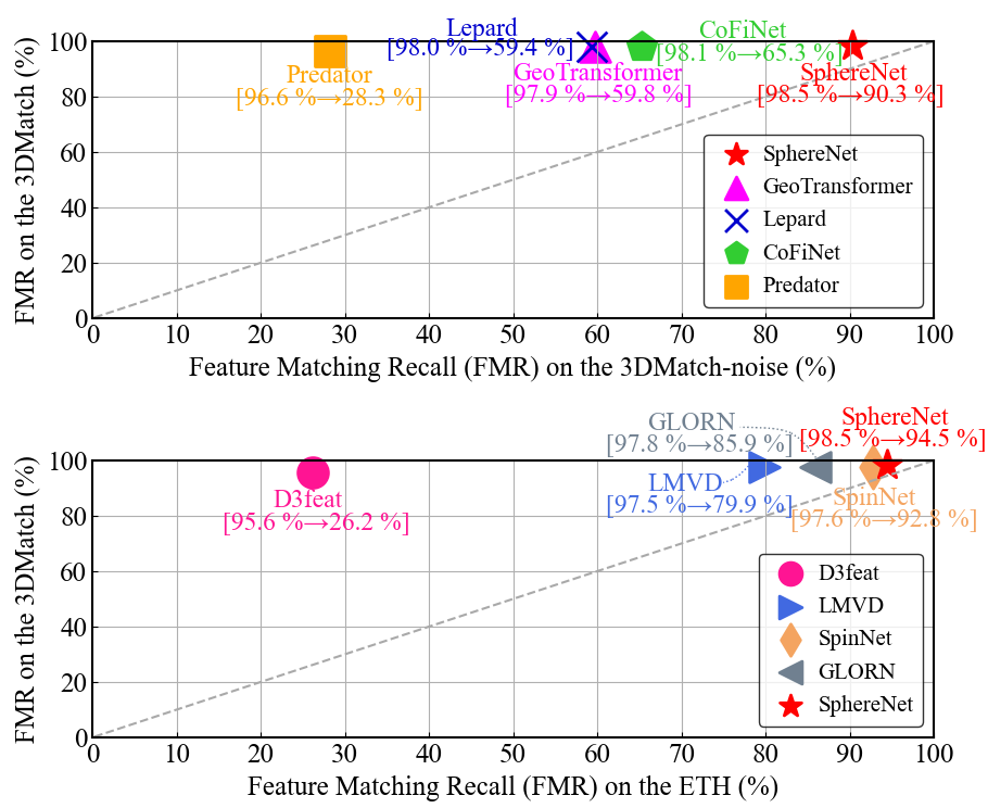
Figure 1: Feature Matching Recall on the 3DMatch [54], ETH dataset [33], and 3DMatch-noise benchmark. Our method not only achieves the highest FMR on 3DMatch, but also has the best generalization ability and anti-noise ability.

Consistently aligning 3D point clouds from different views to the same view is called 3D point cloud registration. As a very important task in computer vision, 3D point cloud registration has a wide range of applications in medical science [22], robotics, and other fields.

Before deep learning was widely used, handcrafted descriptors has played a great role in point cloud registration. In the early years, many handcrafted descriptors such as spin image (SI)[27], point feature histogram (PFH)[39], fast point feature histogram (FPFH)[38], and signature of histogram of orientation (SHOT)[41] are proposed to try to extract local features and geometric information. These traditional methods can extract geometric information and have better interpretability than deep learning. However, in the face of unseen scenes and noisy real scenes, the correct registration is difficult to achieve.

In recent years, deep learning[45] has performed its dominance in various tasks in computer vision. Thanks to deep learning and 3D datasets [54, 33, 17], point cloud registration[24] has developed rapidly, and learning-based methods have flourished. However, the learning-based point cloud registration faces two limitations. First, most of recent works [25, 53, 36, 30, 52, 49] achieve high registration recall scores through a coarse-to-fine framework, but they cannot reject outliers from a coarse scale which leads to false coarse correspondences and false point correspondences. And the scenes with much noise will introduce many outliers. Therefore, they are sensitive to noise and perform poorly in the scenes with large amounts of noise. Second, although the approaches [53, 36, 23] achieve excellent results on 3DMatch and KITTI, they perform poorly on unseen datasets with low generalization ability, which has some limitations in the actual implementation. As a result, the descriptors made by [53, 36, 30, 52, 23] are not robust and general and fails in most scenes with strong noise. In order to solve the adverse effects of noises and outliers on registration, some methods of iniler estimation [48, 55] and outlier removal [47, 6] are proposed. They have greatly improved the accuracy of registration, but most of them are limited to the correspondence filtering, and they do not fundamentally solve the problem in features. In the scenes with strong noise, when the extracted descriptor is affected, these methods [48, 55, 47, 6, 50] can only play a very limited role.

The performance of recent works [3, 53, 36] on 3DMatch is close to reaching saturation, but most works perform poorly in the actual implementation, due to two limitations described above. Therefore, this paper mainly focuses on the anti-noise ability and generalization ability. On this basis, 3DMatch-noise benchmark is proposed to evaluate the anti-noise ability of our method. For this motivation, this paper introduces a new feature extraction method that can learn a noise-robust and unseen-general descriptor for registration in noisy and unseen scenes.

Our method is named SphereNet and consists of two modules. The first is the spheroid generator. It generates a voxel sphere to fully encode the initial geometric feature. In addition, given some ingenious improvements, the module also achieves rotation invariance and anti-noise robustness. The other module is the spherical feature extractor. In this module, we introduce a new spherical convolutional neural network with spherical integrity padding, which fully extracts noise-robust and unseen-general descriptors. Our SphereNet has four key properties: (1) It realizes good anti-noise robustness. In the face of scenes with strong noise, it can also perform well. (2) The descriptor is descriptive and distinctive. (3) It realizes translation and rotation invariance. (4) It has excellent generalization ability on unseen datasets, which is important for implementation in different real-world scenes.

In extensive experiments, our approach achieves the best performance compared with state-of-the-arts [3, 53, 36] in both indoor and outdoor scenes, achieving 93.4% and 75.6% registration recall on the 3DMatch and 3DLoMatch, respectively. As shown in Figure 1, compared with state-of-the-arts [3, 36, 30, 53, 23], the critical advantage of our method are excellent anti-noise robustness and generalization ability. In the scenes with high-intensity noises, our SphereNet improves the feature matching recall by 25.0 percentage points (pp) and the registration recall by 22.2 pp on the challenging 3DMatch-noise benchmark: Noise 1. It also has the best generalization ability with FMR scores of 94.5% and 87.2% on the ETH and KITTI datasets. The main contributions of this paper are as follows:

• We introduce a new method for 3D point cloud registration that can extract a rotation-invariant, noise-robust, and unseen-general descriptor.

• A new benchmark, 3DMatch-noise, is introduced to evaluate the anti-noise robustness of our method. In addition, our method achieves the best anti-noise ability compared with state-of-the-art methods.

• A new feature encoding idea is proposed. The spherical voxelization with spherical interpolation fully encodes the geometric feature, which makes our method more robust to noise.

• A new spherical convolutional neural network is introduced. With spherical integrity padding, it reduces the loss of geometric features and learns a robust and general descriptor.

II Related Work

II-A 3D Handcrafted Descriptors

In the early years, 3D handcrafted descriptors are used to complete the registration based on feature matching. According to the region of the descriptor, it can be divided into global features and local features. The global features describe the whole point cloud, including viewpoint feature histogram (VFH)[1] and clustered viewpoint feature histogram (CVFH)[40]. Local features[19] focus on the local region at the patch level which is better able to describe the local details. Point feature histogram (PFH)[39] and fast point feature histogram (FPFH)[38] describe the local geometric features through the quaternion information of angles and distance. Point pair feature (PPF)[14] extracts features by calculating the normals and relative positions between point pairs. Tombari et al.propose signatures of histograms of orientations (SHOT)[41] based on the point signature (PS)[9], which attempts to fully describe geometric information by constructing spherical domains. With the help of the local reference frame (LRF), SHOT preliminarily realizes rotation invariance, but it is still susceptible to noise. Later, some other manual descriptors [56, 20, 13] based on LRF are proposed. Although they achieve good results in specific scenes, they are less effective in real-world scenes and sensitive to noise.

II-B 3D Learning-based Descriptors

Learning-based registration methods extract descriptors through feature extraction networks, and then use the robust descriptors to register point clouds. Compared with handcrafted descriptors [38, 41, 14, 20], recent learning-based methods [23, 3, 36, 23, 53, 46] have a stronger discriminative ability and generalization ability. The learning-based descriptors can be divided into two categories [2]: patch-based descriptors and fragment-based descriptors.

Patch-based Descriptor.   The input of the patch-based descriptor is the local patch in the scene, while the input of the fragment-based descriptor is the whole fragment. 3DMatch [54] is the pioneering work in patch-based descriptors, which extracts descriptors in the local patches by 3D convolutional neural networks (CNNs). PPFNet [12] combines point pair features with pointnet [34] and is trained by N-tuple loss to complete global matching using local features. Then, PPF-FoldNet[11] improves the invariance against rotation from PPFNet. SpinNet[2, 3] extracts features by cylindrical convolution, which achieves state-of-the-art performance on generalization ability.

Fragment-based Descriptor.   Taking the entire fragment as input, FCGF [8] uses the Minkowski CNNs [7] and the U network [37, 21] to extract a dense feature descriptor. Predator [23] proposes an overlapping region attention module and uses the GNN to extract the local feature, which achieves a great improvement on the 3DLoMatch benchmark and provides a good solution in the scenes with low overlap. GeoTransformer [36] uses the Transformer [44] and superpoint-to-point framework to learn geometric features, which achieves state-of-the-art performance on 3DLoMatch.

Overall, the methods of fragment-based descriptors are much faster than the methods of patch-based descriptors, while the methods of patch-based descriptors can capture local features in detail and have good generalization ability. Unfortunately, both of them are sensitive to noise, and there is not a good way to deal with scenes with strong noise.

III SphereNet

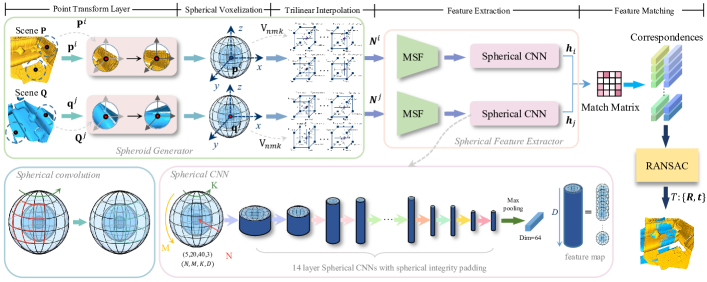
Figure 2: Overall framework of our method. In the spheroid generator, first, the superpoints $\mathbf{p}^{i}$ and $\mathbf{q}^{j}$ are downsampled from the fragments of source $\mathbf{P}$ and target $\mathbf{Q}$. The patches $\mathbf{P}^{i}$ and $\mathbf{Q}^{j}$ are obtained by searching for nearest neighbors at $\mathbf{p}^{i}$ and $\mathbf{q}^{j}$. Second, the point transform layer is used to construct repeatable LRFs for patches $\mathbf{P}^{i}$ and $\mathbf{Q}^{j}$ to realize rotation invariance. In order to improve the ability of noise resistance of the feature, spherical voxelization with spherical interpolation is carried out to encode the initial geometric features $\boldsymbol{N}^{i}$ and $\boldsymbol{N}^{j}$. In the spherical feature extractor, first, by multiscale feature fusion, the generalization ability and anti-density invariance of our SphereNet are improved. After that, spherical CNN with spherical integrity padding is used to extract the robust and general descriptors $\boldsymbol{h_{i}}$ and $\boldsymbol{h_{j}}$. Finally, RANSAC is used to realize global matching to complete the registration.

III-A Problem Statement

For a large-scale scene, two point clouds with overlapping areas are generated from different perspectives, one point cloud is named source $\mathbf{P}=\left\{\mathbf{p}_{i}\in\mathbb{R}^{3}\mid i=1,\ldots,I\right\}$ and another point cloud $\mathbf{Q}=\left\{\mathbf{q}_{j}\in\mathbb{R}^{3}\mid j=1,\ldots,J\right\}$ is named target. The task of registration is to find a rigid transform $\mathbf{T}\{\mathbf{R},\mathbf{t}\}$ where $\mathbf{R}\in SO(3)$ and $\mathbf{t}\in\mathbb{R}^{3}$, which aligns the two point clouds $\mathbf{P}$ and $\mathbf{Q}$. The source is rotated and translated through the rigid transformation $\mathbf{T}$ to obtain the transformed source $\mathbf{T}(\mathbf{P})$, which minimizes the Euclidean distance between the correspondences in the overlapping area of the $\mathbf{T}(\mathbf{P})$ and $\mathbf{Q}$:

$$\underset{\mathbf{R},\mathbf{t}}{\arg\min}\sum_{j=1}^{J}\sum_{i=1}^{I}m_{ij}(\left\|\mathbf{R}\cdot\mathbf{p}_{i}+\mathbf{t}-\mathbf{q}_{j}\right\|_{2}^{2})$$ (1)

where the value of $m_{ij}$ is 0 or 1, which is calculated by

$$m_{ij}=\begin{cases}1&\text{ if }(\mathbf{p}_{i},\mathbf{q}_{j})\in\mathcal{G}\\ 0&\text{ otherwise }\end{cases}$$ (2)

where $\mathcal{G}$ is the set of correspondences between $\mathbf{P}$ and $\mathbf{Q}$. Since the correspondences are unknown, so we should calculate the correspondences by feature matching.

As shown in Figure 2, our SphereNet is a learning-based registration method which will find the correspondences of point pairs with similar features. Through our SphereNet, the feature $\boldsymbol{h}$ is extracted. Then, the point clouds with similar features $\boldsymbol{h}_{\mathbf{p}_{i}}$ and $\boldsymbol{h}_{\mathbf{q}_{j}}$ form a correspondence. Finally, according to the correspondences, the rigid transformation $\mathbf{T}\{\mathbf{R},\mathbf{t}\}$ is calculated by RANSAC.

III-B Spheroid Generator

In order to facilitate the spherical convolutional neural network to fully extract local geometric features, the spheroid generator is introduced. In the spheroid generator, we transform the point cloud of each patch from the global reference frame (GRF) to their local reference frames (LRFs), and disambiguate the direction of the LRFs according to the distribution of point clouds, which greatly improves the repeatability of LRFs. Then, under LRFs, the point cloud in a patch is spherically voxelized, which encodes geometric features. Finally, the robustness of the spherical voxels against noise is improved by spherical interpolation.

Point Transform Layer.   First, a superpoint $\mathbf{p}_{i}\in\mathbf{P}$ in a local region is obtained by random downsampling. By radius search, we search points in sphere $\mathbf{U}_{\mathbf{p}_{i}}^{R}$ to obtain the neighbors $\mathbf{P}^{i}=\{\mathbf{p}_{i_{j}}:\left\|\mathbf{p}_{i_{j}}-\mathbf{p}_{i}\right\|^{2}\leq R\}$ where $R$ is the radius threshold and $\mathbf{p}_{i_{j}}$ is the $j$th neighbor of $\mathbf{p}_{i}$. Then, we use $\mathbf{p}_{i}$ as the reference point to translate $\mathbf{p}_{i_{j}}$ to $\widehat{\mathbf{p}_{i_{j}}}=\mathbf{p}_{i_{j}}-\mathbf{p}_{i}$. LRFs [41] are constructed by decomposing the point covariance matrix $\mathbf{M}$ in $\mathbf{U}_{\mathbf{p}_{i}}^{R}$ to achieve rotation invariance:

$$\mathbf{M}=\sum_{\mathbf{p}_{i_{j}}\in\mathbf{P}^{i}}\frac{\left(R-d_{i_{j}}\right)}{\sum_{\mathbf{p}_{i_{j}}\in\mathbf{P}^{i}}\left(R-d_{i_{j}}\right)}\left(\mathbf{p}_{i_{j}}-\mathbf{p}_{i}\right)\left(\mathbf{p}_{i_{j}}-\mathbf{p}_{i}\right)^{T}$$ (3)

where $d_{i_{j}}$ is the distance between the center point $\mathbf{p}_{i}$ and its $j$th neighbor $\mathbf{p}_{i_{j}}$. Then, the LRFs are constructed by SVD.

Theorem 1

Assume for any rotation transformation $R_{xyz}\in SO(3)$, and any XY-plane rotation transformation $R_{xy|z_{n}}\in SO(2)$ fixed in the direction $z_{n}$. And the transformation $R_{z\rightarrow z_{n}}\in SO(3)$ is obtained through the covariance matrix decomposition, which aligns the point cloud from direction $\mathbf{z}$-axis to $z_{n}$. The linear transformation $\mathcal{L}(\cdot)$ of the point transform layer maps the local patch $\mathbf{P}^{i}$ to $\widehat{\mathbf{P}^{i}}:\mathbb{R}^{3\times\left|\mathbf{P}^{i}\right|}\rightarrow\mathbb{R}^{3\times\left|\mathbf{P}^{i}\right|}$, then there is an equivariant relation $\mathcal{L}(R_{xyz}\circ\mathbf{p}^{i})=R_{xy|z_{n}}\circ\mathbf{p}^{i}$.

Proof:

According to the principle of rotation invariance, the matrix of linear transformation $\mathcal{L}(\mathbf{P}^{i})$ is expressed as $R^{-1}_{z\rightarrow z_{n}}\circ\mathbf{P}^{i}=R_{z_{n}\rightarrow z}\circ\mathbf{P}^{i}$, where $\mathbf{z}$ is the direction vector of the z-axis of the GRFs and $z_{n}$ is the $\mathbf{z}$ direction vector of the z-axis of LRFs. Thus, we have:

$$\mathcal{L}(R_{xyz}\circ\mathbf{P}^{i}) =R^{-1}_{z_{\rightarrow}z_{n}}\circ(R_{xyz}\circ\mathbf{P}^{i})$$ (4)

$$=R_{z_{n}\rightarrow z}\circ(R_{xyz}\circ\mathbf{P}^{i})$$

$$=(R_{z_{n}\rightarrow z}\cdot R_{xyz})\circ\mathbf{P}^{i}$$

$$=R_{xy|z_{n}}\circ\mathbf{P}^{i}$$

∎

Spherical Voxelization.   Inspired by [16, 28, 41], the sphere domain $\mathbf{U}_{\mathbf{p}_{i}}^{R}$ is divided into $N\times M\times K$ small voxels $\mathbf{V}_{nmk}$ from three directions: radius length $r=\sqrt{x^{2}+y^{2}+z^{2}}$, elevation angle $\theta=\arccos\frac{z}{\sqrt{x^{2}+y^{2}+z^{2}}}$ and azimuth angle $\varphi=\arctan\frac{y}{x}$, where $n\in\{0,\ldots,N\}$ $m\in\{0,\ldots,M\}$ and $k\in\{0,\ldots,K\}$ are indexes of $r$, $\theta$ and $\varphi$, respectively. The voxel boundary sets $S_{r}$, $S_{\theta}$, and $S_{\varphi}$ of radius length $r$, elevation angle $\theta$, and azimuth angle $\varphi$ are defined as follows:

$$\begin{cases}S_{r}&=\{r_{n}:r_{0}+n\cdot\frac{r_{N}-r_{0}}{N}\}\\ S_{\theta}&=\{\theta_{m}:\theta_{0}+m\cdot\frac{\theta_{M}-\theta_{0}}{M}\}\\ S_{\varphi}&=\{\varphi_{k}:\varphi_{0}+k\cdot\frac{\varphi_{K}-\varphi_{0}}{K}\}\end{cases}$$ (5)

where $r_{0}=0$, $\theta_{0}=0$ and $\varphi_{0}=0$ are the first items of the three boundary sets and $r_{N}=R$, $\theta_{M}=\pi$ and $\varphi_{K}=2\pi$ are the last items. By the boundary value sets $S_{r}$, $S_{\theta}$, $S_{\varphi}$, the sphere domain $\mathbf{U}_{\mathbf{p}_{i}}^{R}$ is voxelized to small voxels $\mathbf{V}_{nmk}$ and the points $\mathbf{P}^{i}_{nmk}$ in the voxel $\mathbf{V}_{nmk}\in\mathbf{U}_{\mathbf{p}_{i}}^{R}$ is defined as follows:

$$\{\mathbf{p}_{i_{j}}:\!(r_{n\!-\!1},\theta_{m\!-\!1},\varphi_{k\!-\!1})\!\leqslant\!(r^{i}_{j},\theta^{i}_{j},\varphi^{i}_{j})\!<\!(r_{n},\theta_{m},\varphi_{k})\}$$ (6)

where $(a_{1},b_{1},c_{1})<(a_{2},b_{2},c_{2})$ is equal to $(a_{1}\!<\!a_{2})\land(b_{1}\!<\!b_{2})\land(c_{1}\!<\!c_{2})$. Finally, the number $N_{nmk}=|\mathbf{P}^{i}_{nmk}|$ in the voxel $\mathbf{V}_{nmk}$ is counted as our initial description of geometric information.

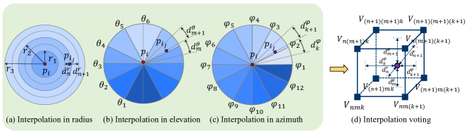
Figure 3: Illustration of spherical interpolation based on spherical voxelization.

Spherical Interpolation.   Theoretically, the greater number of spherical voxels, the finer feature we obtain. However, considering the universality of features and the real-time performance of the algorithm, we have to reduce the number of spherical voxels. In addition, due to the large amount of noise in the actual scenes, many points $\mathbf{p}_{i_{j}}\in\mathbf{V}_{n_{1}m_{1}k_{1}}$ affected by noise $\boldsymbol{\varepsilon}$ may be allocated to another specific small voxel $\mathbf{p}_{i_{j}}+\boldsymbol{\varepsilon}\in\mathbf{V}_{n_{2}m_{2}k_{2}}$ which finally causes the error of our initial feature. Therefore, in order to overcome the influence of noise and extract finer features under a few voxels, this paper proposes a spherical interpolation method. By this method, each point in each voxel is interpolated in the three dimensions of radius length $r$, elevation angle $\theta$ and azimuth angle $\varphi$ respectively. Illustration of spherical interpolation based on spherical voxelization is shown in Figure 3.

Interpolation in radius length. As shown in Figure 3 (a), the $N+1$ boundary values in the boundary set $S_{r}$ divide the whole sphere into $N$ regions in the dimension of radius length. In each region $n$, the region centerline (the dotted lines in Figure 3) can be calculated as $\frac{(r_{n}+r_{n-1})}{2}$. Then, the interpolation weight $w^{r}_{n}$ from point $\mathbf{p}_{i_{j}}$ to region $n$ is given by the following equation:

$$w^{r}_{n}=\begin{cases}1-\frac{d^{r}_{n}}{r_{N}/N}&,\quad d^{r}_{n}<\frac{r_{N}}{N}\wedge r^{i}_{j}\geqslant\frac{r_{N}}{2N}\\ 1&,\quad d^{r}_{n}<\frac{r_{N}}{N}\wedge r^{i}_{j}<\frac{r_{N}}{2N}\\ 0&,\quad d^{r}_{n}\geqslant\frac{r_{N}}{N}\end{cases}$$ (7)

where $d^{r}_{n}=|\frac{(r_{n}+r_{n-1})}{2}-r^{i}_{j}|$ is the distance between point $\mathbf{p}_{i_{j}}$ and the region centerline of region $n$, and $n\in\{1,\ldots,N\}$.

Interpolation in elevation angle. As shown in Figure 3 (b), the $M+1$ boundary values in the boundary set $S_{\theta}$ divide the whole sphere into $M$ regions in the dimension of elevation angle $\theta$. In each region $m$, the region centerline can be calculated as $\frac{(\theta_{m}+\theta_{m-1})}{2}$. Therefore, the interpolation weight $w^{\theta}_{m}$ from point $\mathbf{p}_{i_{j}}$ to region $m$ is given by the following equation:

$$w^{\theta}_{m}=\begin{cases}1-\frac{d^{\theta}_{m}}{{\theta_{M}}/{M}}\!&,\!\quad d^{\theta}_{m}<\frac{\theta_{M}}{M}\wedge\theta_{M}-\frac{\theta_{M}}{2M}\geqslant\theta^{i}_{j}\geqslant\frac{\theta_{M}}{2M}\\ 1\!&,\!\quad d^{\theta}_{m}<\frac{\theta_{M}}{M}\wedge\theta^{i}_{j}<\frac{\theta_{M}}{2M}\\ 1\!&,\!\quad d^{\theta}_{m}<\frac{\theta_{M}}{M}\wedge\theta^{i}_{j}>\theta_{M}-\frac{\theta_{M}}{2M}\\ 0\!&,\!\quad d^{\theta}_{m}\geqslant\frac{\theta_{M}}{M}\end{cases}$$ (8)

where $d^{r}_{n}=|\frac{(\theta_{m}+\theta_{m-1})}{2}-\theta^{i}_{j}|$ is the distance between point $\mathbf{p}_{i_{j}}$ and the region centerline of region $m$, and $m\in\{1,\ldots,M\}$.

Interpolation in azimuth angle. The interpolation weight $w^{\varphi}_{k}$ from point $\mathbf{p}_{i_{j}}$ to region $k$ is given by the following equation:

$$w^{\varphi}_{k}=\begin{cases}1-\frac{d^{\varphi}_{k}}{\varphi_{K}/K}&,\quad d^{\varphi}_{k}<\frac{\varphi_{K}}{K}\\ 0&,\quad d^{\varphi}_{k}\geqslant\frac{\varphi_{K}}{K}\end{cases}$$ (9)

where $d^{\varphi}_{k}=|\frac{(\varphi_{k}+\varphi_{k-1})}{2}-\varphi^{i}_{j}|$ is the distance between point $\mathbf{p}_{i_{j}}$ and the region centerline of region $k$, and $k\in\{1,\ldots,K\}$.

Then, according to the weights $w^{r}_{n}$, $w^{\theta}_{m}$, and $w^{\varphi}_{k}$ in three dimensions, the number $N^{j}_{nmk}$ that the $j$th neighbor $\mathbf{p}_{i_{j}}$ interpolated into the small voxel $\mathbf{V}_{nmk}$, can be calculated:

$$N^{j}_{nmk}=w^{r}_{n}\times w^{\theta}_{m}\times w^{\varphi}_{k}$$ (10)

As shown in Figure 3 (d), each point casts interpolation votes to the $2\times 2\times 2$ nearest voxels (the eight vertices of the voxel). Finally, the initial geometric features are encoded by summing the number of votes for each small voxel:

$$N_{nmk}=\sum_{\mathbf{p}_{i_{j}}\in\mathbf{P}_{i}}N^{j}_{nmk}$$ (11)

Theorem 2

Given any XOY-plane rotation transformation $R_{xy|z_{n}}\in SO(2)$ fixed in the direction $\mathbf{z}_{n}$ and defined the neighbors $\mathbf{P}^{i}$ in the voxel $\mathbf{V}^{i}_{nmk}$ as $\mathbf{P}^{i}_{nmk}\subseteq\mathbf{P}^{i}$, then the spherical voxelization with spherical interpolation is an equivariant mapping $\mathcal{H}(\cdot)$ of the transformation $R_{xy|z_{n}}$.

Proof:

Let $\mathcal{H}(\cdot)$ be a mapping from $\mathbf{P}^{i}$ after the point transform layer and direction disambiguation to the initial feature $\mathbf{N}^{i}=\{\mathbf{N}^{i}_{111},\ldots,\mathbf{N}^{i}_{nmk},\ldots,\mathbf{N}^{i}_{NMK}\}$ in spherical voxel $\mathbf{V}^{i}$: $\mathbb{R}^{3\times\left|\mathbf{P}^{i}\right|}\rightarrow\mathbb{R}^{N\times M\times K}$. Since the rotation transformation $R_{xy|z_{n}}$ is only in the XOY-plane, the points $\mathbf{P}^{i}_{nmk}$ located in small voxels will be rotated to $\mathbf{P}^{i}_{nm(k+\zeta)}$ with the same radius length $r$, elevation angle $\theta$ and different azimuth angle $\varphi$, where $\zeta$ is related to the rotation angle in the XOY-plane. Further derivation, we can obtain:

$$\mathbf{R}_{xy|z_{n}}\circ\mathbf{P}^{i}_{nmk}=\mathbf{P}^{i}_{nm(k+\zeta)}$$ (12)

$$\mathbf{R}_{xy|z_{n}}\cdot\boldsymbol{N}^{i}_{nmk}=\boldsymbol{N}^{i}_{nm(k+\zeta)}$$

where $\boldsymbol{N}^{i}_{nmk}$ is the number of points located in the voxel $\mathbf{V}^{i}_{nmk}$ after interpolation and it has the same position information as $\mathbf{V}^{i}_{nmk}$. Therefore, $\mathbf{R}_{xy|z_{n}}$ is the transformation of the position in $\mathbf{V}^{i}_{nmk}$, and $\boldsymbol{N}^{i}_{nm(k+\zeta)}$ is the number of points under the new voxel $\mathbf{V}^{i}_{nm(k+\zeta)}$. According to Eq. 12, we have completed the derivation of Lemma 2:

$$\mathbf{R}_{xy|z_{n}}\circ\mathcal{H}\left(\mathbf{P}^{i}\right)=\mathbf{R}_{xy|z_{n}}\circ\boldsymbol{N}^{i}$$ (13)

$$=\mathbf{R}_{xy|z_{n}}\circ\left[\boldsymbol{N}^{i}_{111},\ldots,\boldsymbol{N}^{i}_{nmk},\ldots,\boldsymbol{N}^{i}_{NMK}\right]$$

$$=\left[\boldsymbol{N}^{i}_{11(1+\zeta)},\ldots,\boldsymbol{N}^{i}_{nm(k+\zeta)},\ldots,\boldsymbol{N}^{i}_{NM(K+\zeta)}\right]$$

$$=\mathcal{H}\left(\mathbf{P}^{i}_{nm(k+\zeta)}\right)=\mathcal{H}\left(\mathbf{R}_{xy|z_{n}}\circ\mathbf{P}^{i}\right)$$

∎

Multiscale Feature Fusion.   In different datasets, the density of the point cloud is different. To resist the impact on density and improve the generalization ability of our SphereNet on cross-source datasets, we follow PointNet++ [35] and perform multiscale feature fusion on our spherical voxels. As shown in Figure 4, we use three radii to obtain three spherical voxels at different scales. Then, the three are concatenated on the feature channel to complete the multiscale fusion, which can be described as a mapping $\mathcal{M}(\cdot):\mathbb{R}^{N\times M\times K}\rightarrow\mathbb{R}^{3\times\frac{N}{3}\times M\times K}$.

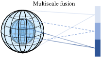
Figure 4: Illustration of multiscale feature fusion.

III-C Spherical Feature Extractor

For spherical feature extractor, we don’t follow spherical CNN [10] or SpinNet [3]. Instead, we use a simple and efficient 3D sphere flattening to form 2D map, and then carried out 2D convolution with a sphere, which is very suitable for deep extraction of our initial features. Compared with recent methods [23, 53, 36] that take KPConv [43] as a backbone, our network design provides a new idea for unseen-general and noise-robust descriptor extraction.

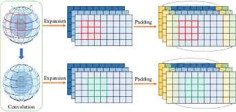
Figure 5: Spherical convolution and boundary padding.

Spherical Convolution.   Before our work, many scholars have done research [10, 15, 26, 28] on spherical convolution. Huan et al.[28] propose an Octree-guided CNN by combining CNN with Octree. And Taco et al.[10] pioneered the feasibility of spherical convolutions and applied FFT to spherical convolutions. Different from the two methods, our SphereNet creatively proposes a new 3D spherical convolution and spherical integrity padding method, whose working principle can be compared with the projection expansion of the earth map, flattening the voxel sphere and obtaining a 3D tensor similar to a cuboid as shown in Figure 5. Therefore, convolution is carried out on the flattened tensor through a 3D convolution kernel.

Spherical Integrity Padding.   Because the voxel sphere is cut lengthwise at azimuth angle $\varphi=0^{\circ}$ to flatten the sphere, the left and right boundaries in the 3D tensor are furthest apart, while the boundaries are adjacent to each other in the spherical voxels, which is bound to lead to the loss of geometric information. Therefore, we propose a spherical integrity padding to ensure that complete geometric features can be extracted from the boundaries. As shown in Figure 5, the left and right boundaries after spherical flattening are padded with each other every time 3D convolution.

Spherical CNN.   In the spheroid generator, we have already discretized a large number of points into the sphere with many small voxels. The ordered voxel sphere is very suitable for the implementation of the spherical convolutional neural network (Spherical CNN). By Spherical CNN, the mapping $\mathcal{F}(\cdot)$ between the input and output feature maps $\boldsymbol{h}$ of each layer is shown in the following equation:

$$\mathcal{F}(\boldsymbol{h}_{nmk}^{d})=\sum_{d=1}^{D}\sum_{r=1}^{a}\sum_{\theta=1}^{b}\sum_{\varphi=1}^{c}\boldsymbol{\omega}_{r\theta\varphi}^{d^{\prime}d}\boldsymbol{h}_{(n+r)(m+\theta)(k+\varphi)}^{d}$$ (14)

where $a$, $b$, $c$, $D$ are the size and number of the convolution filter $\Omega\in\mathbb{R}^{a\times b\times c}$ , and $\boldsymbol{\omega}_{r\theta\varphi}^{d^{\prime}d}$ is a learnable parameter in the convolution kernel where $d$ and $d^{\prime}$ are the number of input and output channels, respectively. The rotation invariance of the end-to-end model is proved in 4.

Theorem 3

Given any XOY-plane rotation transformation $R_{xy|z_{n}}\in SO(2)$ fixed on the direction $\mathbf{z}_{n}$, then the Spherical CNN is an equivariant mapping $\mathcal{F}(\cdot)$ of the transformation $R_{xy|z_{n}}$.

Proof:

According to Eq. 11 (in our paper), the spherical CNN can regarded as a mapping $\mathcal{F}(\cdot)$ that transforms from one feature map $\boldsymbol{h}_{nmk}^{d}$ to another $\boldsymbol{h}_{nmk}^{d^{\prime}}$. When the transformation $R_{xy|z_{n}}$ is performed on $\boldsymbol{h}_{nmk}^{d}$, since the transformation is only in the XOY-plane, the feature $\boldsymbol{h}_{nmk}^{d}$ will be transformed into $\boldsymbol{h}_{nm(k+\zeta)}$. Therefore, the equivariant mapping of the transformation $R_{xy|z_{n}}$ can be proved as follows:

$$\mathcal{F}(R_{xy|z_{n}}\circ\boldsymbol{h}_{nmk}^{d})=\mathcal{F}(\boldsymbol{h}_{nm(k+\zeta)})=R_{xy|z_{n}}\circ\mathcal{F}(\boldsymbol{h}_{nmk}^{d})$$ (15)

∎

Theorem 4

Given any rotation transformation $R_{xyz}\in SO(3)$, the end-to-end framework of feature extraction is an invariant mapping.

Proof:

Firstly, it is known that maximum pooling has invariance. So we can get the following property:

$$\mathcal{O}(\boldsymbol{h}_{nmk}^{d})=\mathcal{O}(R_{xy|z_{n}}\circ\boldsymbol{h}_{nmk}^{d})$$ (16)

Then, according to the properties we proved in Lemma 1, 2, 3 we can derive the end-to-end framework of feature extraction step by step:

$$(\mathcal{O}\star\mathcal{F}\star\mathcal{H}\star\mathcal{L})(R_{xyz}\circ\mathbf{P}^{i})$$ (17)

$$=\mathcal{O}(\mathcal{F}(\mathcal{H}(\mathcal{L}(R_{xyz}\circ\mathbf{P}^{i}))))$$

$$=\mathcal{O}(\mathcal{F}(\mathcal{H}(R_{xy|z_{n}}\circ\mathcal{L}(\mathbf{P}^{i}))))$$

$$=\mathcal{O}(\mathcal{F}(R_{xy|z_{n}}\circ\mathcal{H}(\mathcal{L}(\mathbf{P}^{i}))))$$

$$=\mathcal{O}(R_{xy|z_{n}}\circ\mathcal{F}(\mathcal{H}(\mathcal{L}(\mathbf{P}^{i}))))$$

$$=\mathcal{O}(\mathcal{F}(\mathcal{H}(\mathcal{L}(\mathbf{P}^{i}))))$$

where mapping $\mathcal{O}(\cdot)$ is the maximum pooling, $(\mathcal{O}\star\mathcal{F}\star\mathcal{H}\star\mathcal{L})(\cdot)$ is the mapping of the whole framework and operation $\star$ is the composite product between two transformations. ∎

III-D Detailed Network Architecture

The detail network structure of our SphereNet is shown in Figure 6. Our model is mainly based on Spherical convolution (SConv) proposed in this paper, and SConv combines with conv2d to form the network of our SphereNet. The spherical integrity padding is conducted before each convolution. As shown in Figure 6, we provide two different network structures. The first network (top) does not use the MSF module and is trained from the 3DMatch dataset for direct testing on the 3DMatch dataset. The second network (middle) uses MSF to improve the generalization ability of our model. After experimental comparative analysis, the second model has better generalization ability and can be used for generalization between different datasets.

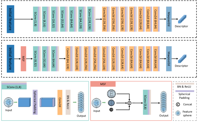
Figure 6: Detail network structure of our SphereNet.

III-E Loss Function

Our method is patch-learning and we choose the hardest-in-batch approach[32] for the design of the loss function. During training, a batch $\mathcal{B}=(\mathcal{P},\mathcal{Q})$ is given by the combination of Source $\mathcal{P}$ and Target $\mathcal{Q}$, where the patch $\mathbf{P}_{i}\in\mathcal{P}$, patch $\mathbf{Q}_{i}\in\mathcal{Q}$, and $(\mathbf{P}_{i},\mathbf{Q}_{i})\in\mathcal{G}$, $(i=1,2,\cdots n)$. The hardest-in-batch contrastive margin loss $\mathcal{L}_{cm}$ is defined as:

$$\mathcal{L}_{cm} =\frac{1}{|\mathcal{P}|}\sum_{\mathbf{P}_{i}\in\mathcal{P}}\left(\max\left[\left(\max d^{\mathbf{h}}_{i}-\Delta_{p}\right),0\right]\right.$$ (18)

$$\left.+\max\left[\left(\Delta_{n}-\min d^{\mathbf{h}}_{ij}\right),0\right]\right)$$

where $d^{\mathbf{h}}_{i}=\|\mathbf{h}_{\mathbf{P}_{i}}-\mathbf{h}_{\mathbf{Q}_{i}}\|_{2}$ is the feature distance between $\mathbf{P}_{i}$ and $\mathbf{Q}_{i}$ and $d^{\mathbf{h}}_{ij}=\|\mathbf{h}_{\mathbf{P}_{i}}-\mathbf{h}_{\mathbf{Q}_{j}}\|_{2}$ is the feature distance between $\mathbf{P}_{i}$ and $\mathbf{Q}_{j}$. $\Delta_{p}$ and $\Delta_{n}$ is the positive and negative margin of the feature distance, respectively.

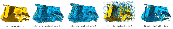
Figure 7: Examples in the 3DMatch-noise benchmark with different noises. The yellow point clouds are the original data of the 3DMatch dataset, and the blue point clouds are the noise point clouds in the 3DMatch-noise benchmark.

IV Experiments

This paper evaluates on two distinct datasets for indoor and outdoor scenes. For indoor scenes, we used the RGB-D reconstructed dataset 3DMatch[54] to verify that our method achieved the best performance in indoor scenes. It is also evaluated on the KITTI [17] and ETH [33] datasets. Our approach is also competitive in outdoor scenes. It is worth noting that we also evaluate our SphereNet on the 3DMatch-noise benchmark proposed in this paper.

IV-A Experimental Setup

First, we downsample the point cloud and generate patches as the input of our method. Then, we can use our spheroid generator and spherical feature extractor to extract the 3D feature descriptors. Finally, the extracted descriptors are used for registration by using 50k RANSAC. We implement our SphereNet in the PyTorch framework and choose Adam as our optimizer. We set the initial value of the learning rate to 0.001 and decrease it by 50% with each 5 epochs. The batch size and training epoch are set to 64 and 30, respectively. Finally, one of the training models with the best performance in validation is selected as our pretraining model. All experiments are conducted on the Arch Linux system with an NVIDIA RTX 2080Ti GPU.

Hyperparameter Settings.   Here are the detailed hyperparameter settings in this section. For different datasets and different experiments, the hyperparameters set in the experiment are given in Table I. It is worth noting that in all experiments, we set the number of spherical voxels as $15\times 20\times 40$. However, in order to overcome the scale inconsistency between different datasets, we adjusted the radius threshold $R$ of constructing LRFs through the ablation experiment. For 3DMatch dataset, $R$ is to 0.3m because the indoor point clouds are dense. For the ETH and KITTI datasets, respectively, because the outdoor point clouds are sparse, $R$ are set to 1.2m and 3.0m. In addition, in order to improve the generalization ability of cross-dataset registration, multiscale feature fusion (MSF) is used in some generalization experiments.

TABLE I: Hyperparameter settings of our SphereNet.

Dataset	$N$	$M$	$K$	$R$	MSF
3DMatch	15	20	40	0.3m	NO
KITTI	15	20	40	2.0m	NO
3DMatchToETH	15	20	40	1.2m	YES
3DMatchToKITTI	15	20	40	3.0m	YES

IV-B Evaluation on 3DMatch & 3DLoMatch

Dataset and Metrics.   Following previous works [4, 3], we used 46 scenes for training, 8 scenes for validation, and 8 scenes for testing. On 3DMatch, we evaluate on three benchmarks: (1) the 3DMatch benchmark is tested on scenes with more than 30% overlap on the 3DMatch dataset; (2) the 3DLoMatch benchmark is tested on scenes with $10\%\thicksim 30\%$ overlap; (3) the 3DMatch-noise benchmark is tested on the 3DMatch dataset with strong noise.

Following [4, 53], we evaluated the performance by three evaluation metrics: Registration Recall (RR), Inlier Ratio (IR), and Feature Matching Recall (FMR).

Feature Matching Recall is the fraction of two point clouds whose Inlier Ratio (IR) is above the threshold $\tau_{2}=5\%$. So we should calculate IR before FMR. First, we obtain the point pair correspondences $\left(\mathbf{p}_{i},\mathbf{q}_{j}\right)\in\boldsymbol{\Omega}_{h}$ between two point clouds $\mathbf{P}$ and $\mathbf{Q}$ by feature matching. Then, $\mathbf{P}$ and $\mathbf{Q}$ are aligned according to the ground-truth transformation $\mathbf{T_{h}}\{\mathbf{R_{h}},\mathbf{t_{h}}\}$. Finally, the Euclidean distance between the aligned point pair $\left(\mathbf{p}_{i},\mathbf{q}_{j}\right)$ is calculated. If the distance is less than the threshold $\tau_{1}=0.1$m, the point pair $\left(\mathbf{p}_{i},\mathbf{q}_{j}\right)$ is considered as inlier point pair. IR is the ratio of the number of inlier point pairs to the number of correspondences:

$$\mathrm{IR}=\frac{1}{\left|\boldsymbol{\Omega}_{h}\right|}\sum_{\left(\mathbf{p}_{i},\mathbf{q}_{j}\right)\in\boldsymbol{\Omega}_{h}}\mathbbm{1}\left(\left\|\mathbf{T_{h}}(\mathbf{p}_{i})-\mathbf{q}_{j}\right\|_{2}<\tau_{1}\right)$$ (19)

where $\left|\boldsymbol{\Omega}_{h}\right|$ is the number of correspondences and $\mathbbm{1}$ is an indicator function. $\mathbf{T}(\mathbf{p}_{i})$ is the point through the ground-truth transformation $\mathbf{T_{h}}$ from $\mathbf{p}_{i}$. $\|\cdot\|_{2}$ denotes the Euclidean distance.

When the IR between two point clouds is above the threshold $\tau_{2}=5\%$, we believe that the feature matching of two point clouds is successful. Finally, FMR is the percentage of point clouds that IR exceeds the threshold $\tau_{2}=5\%$:

$$\mathrm{FMR}=\frac{1}{H}\sum_{h=1}^{H}\mathbbm{1}\left(\mathrm{IR_{h}}>\tau_{2}\right)$$ (20)

where $H$ is the total number of point cloud pairs.

Registration Recall is the fraction of correctly registered point cloud pairs. First, we should calculate the RMSE which determines whether the registration of two point clouds $\mathbf{P}$ and $\mathbf{Q}$ is successful.

$$\operatorname{RMSE}=\sqrt{\frac{1}{\left|\boldsymbol{\Omega}_{h}\right|}\sum_{\left(\mathbf{p}_{i},\mathbf{q}_{j}\right)\in\boldsymbol{\Omega}_{h}}\left\|\mathbf{T_{h}}(\mathbf{p}_{i})-\mathbf{q}_{j}\right\|_{2}^{2}}$$ (21)

If the RMSE is less than the threshold $\tau_{3}=0.2$m, the registration of point clouds $\mathbf{P}$ and $\mathbf{Q}$ is regarded as successful. Therefore, RR is calculated by the following equation:

$$\mathrm{RR}=\frac{1}{H}\sum_{h=1}^{H}\mathbbm{1}\left(\mathrm{RMSE}_{h}<\tau_{3}\right)$$ (22)

TABLE II: Evaluation results on 3DMatch and 3DLoMatch.

	3DMatch					3DLoMatch
# Samples	5000	2500	1000	500	250	5000	2500	1000	500	250
Feature Matching Recall (%) $\uparrow$
PerfectMatch [18]	95.0	94.3	92.9	90.1	82.9	63.6	61.7	53.6	45.2	34.2
FCGF [8]	97.4	97.3	97.0	96.7	96.6	76.6	75.4	74.2	71.7	67.3
D3Feat [4]	95.6	95.4	94.5	94.1	93.1	67.3	66.7	67.0	66.7	66.5
SpinNet [3]	97.6	97.2	96.8	95.5	94.3	75.3	74.9	72.5	70.0	63.6
Predator [23]	96.6	96.6	96.5	96.3	96.5	78.6	77.4	76.3	75.7	75.3
YOHO [46]	98.2	97.6	97.5	97.7	96.0	79.4	78.1	76.3	73.8	69.1
CoFiNet [53]	98.1	98.3	98.1	98.2	98.3	83.1	83.5	83.3	83.1	82.6
GeoTransformer [36]	97.9	97.9	97.9	97.9	97.6	88.3	88.6	88.8	88.6	88.3
SphereNet1 (ours)	98.2	98.3	98.2	97.3	95.8	79.1	78.5	77.3	74.1	68.4
SphereNet2 (ours)	98.5	98.3	98.3	98.3	98.0	88.8	87.0	86.2	83.1	82.0
Registration Recall (%) $\uparrow$
PerfectMatch [18]	78.4	76.2	71.4	67.6	50.8	33.0	29.0	23.3	17.0	11.0
FCGF [8]	85.1	84.7	83.3	81.6	71.4	40.1	41.7	38.2	35.4	26.8
D3Feat [4]	81.6	84.5	83.4	82.4	77.9	37.2	42.7	46.9	43.8	39.1
SpinNet [3]	88.6	86.6	85.5	83.5	70.2	59.8	54.9	48.3	39.8	26.8
Predator [23]	89.0	89.9	90.6	88.5	86.6	59.8	61.2	62.4	60.8	58.1
YOHO [46]	90.8	90.3	89.1	88.6	84.5	65.2	65.5	63.2	56.5	48.0
CoFiNet [53]	89.1	88.9	88.4	87.4	87.0	67.5	66.2	64.2	63.1	61.0
GeoTransformer [36]	92.0	91.8	91.8	91.4	91.2	75.0	74.8	74.2	74.1	73.5
SphereNet1 (ours)	91.2	90.3	88.8	86.2	77.7	60.0	59.6	53.9	45.5	32.4
SphereNet2 (ours)	93.4	93.5	93.0	92.4	89.8	75.6	71.2	70.0	70.6	65.9

Correspondence Results.   Following [53, 3], we first compare the correspondence results of our method with the state-of-the-art methods [18, 8, 4, 3, 23, 46, 2, 53] in Table II. To verify the robustness to samplings, we set up experiments with sampling numbers 5000, 2500, 1000, 500 and 250. For keypoint sampling, we provide two versions of SphereNet. The first is our SphereNet¹, which uses random downsampling to obtain keypoints; the second is SphereNet², where we add the keypoint detection module of Predator [23] into our framework to obtain keypoints. For FMR, our SphereNet² achieves the best FMR scores of 98.5% and 88.8% on 3DMatch and 3DLoMatch, respectively. Additionally, our SphereNet¹ without keypoint detection or coarse-to-fine matching [53, 36] also achieves the highest FMR than the methods [23, 2, 53].

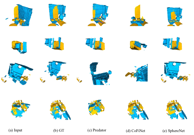
Figure 10: Registration results on the 3DMatch and 3DLoMatch datasets.

Registration Results.   50k RANSAC is used to calculate the transformation through feature matching. Notably, whether on the 3DMatch or 3DLoMatch dataset, our SphereNet² has the best performance for any number of keypoints. It attains a new state-of-the-art result of 93.4%, a 4.8 percentage points (pp) increase compared with baseline SpinNet [3] on 3DMatch. For 3DLoMatch, our SphereNet² also achieves the best RR score of 75.6%. Moreover, with the decrease in the sampling numbers, the decrease in RR of our method is small, which means that our method has good stability under different samplings. As the qualitative results on 3DMatch shown in Figure 10, our SphereNet achieves successful registration in some examples where other methods [23, 53] fail.

We also conduct detailed experiments for each scene under the 3DMatch and 3DMatch-noise datasets (introduced in Section IV-D). Following [3], we calculated RR for each scene to evaluate the performance, and the results are shown in Table III. As can be seen from the Table III, compared with the baselines, the performance of our method in each scene has been greatly improved. In particular, due to the characteristics of our method, the performance is significantly improved in all scenes on the 3DMatch-noise dataset with strong noise.

TABLE III: Scene-wise registration results on the 3DMatch and 3DMatch-noise datasets.

Model	3DMatch									3DMatch-noise
	Kitchen	Home_1	Home_2	Hotel_1	Hotel_2	Hotel_3	Study	Lab	Mean	Kitchen	Home_1	Home_2	Hotel_1	Hotel_2	Hotel_3	Study	Lab	Mean
Registration Recall (%) $\uparrow$
3DSN [18]	90.6	90.6	65.4	89.6	82.1	80.8	68.4	60.0	78.4	-	-	-	-	-	-	-	-	-
FCGF [8]	98.0	94.3	68.6	96.7	91.0	84.6	76.1	71.1	85.1	-	-	-	-	-	-	-	-	-
D3Feat [4]	96.0	86.8	67.3	90.7	88.5	80.8	78.2	64.4	81.6	-	-	-	-	-	-	-	-	-
Predator [23]	97.6	97.2	74.8	98.9	96.2	88.5	85.9	73.3	89.0	42.3	41.5	28.9	48.4	39.7	61.5	45.3	46.7	44.3
CoFiNet [53]	96.4	99.1	73.6	95.6	91.0	84.6	89.7	84.4	89.3	57.2	58.5	39.0	65.4	53.8	50.0	51.3	46.7	52.7
GeoTransformer [36]	98.9	97.2	81.1	98.9	89.7	88.5	88.9	88.9	91.5	56.3	57.6	40.3	65.2	55.2	52.6	44.9	41.5	51.7
SphereNet1 (ours)	98.2	95.3	74.2	99.5	93.6	92.3	82.9	75.6	91.2	55.5	59.4	43.4	56.6	43.6	57.7	57.3	48.9	53.8
SphereNet2 (ours)	98.9	96.2	80.5	98.9	93.6	88.5	87.6	88.9	93.4	78.6	82.1	55.4	81.9	66.7	73.1	78.2	60.0	74.9

Repeatability for Different Thresholds.   We also set different thresholds to verify the robustness to the thresholds $\tau_{1}$ and $\tau_{2}$. As shown in Figure 8, compared with other methods [23, 3, 38, 41, 54, 4], our SphereNet achieves the best results at all different thresholds. Under the stricter condition $\tau_{1}=0.2$, the FMR obtained by our SphereNet is $89.5\%$, while other methods [54, 4] have a significant decline. Therefore, our method has good stability and can achieve good results even in the face of strict conditions.

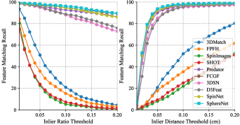
Figure 8: Feature Matching Recall on the 3DMatch dataset under different inlier distance threshold $\tau_{1}$ and inlier ratio threshold $\tau_{2}$.

Rotation Invariance.   Following [4, 3], we build a rotated 3DMatch benchmark by applying arbitrary rotations in SO(3) group to all fragments of the 3DMatch dataset. On the rotated 3DMatch benchmark, the FMR scores are calculated by our method and other strong baselines [8, 4, 46, 36, 3] to verify the rotation invariance of our SphereNet. As is shown in Table IV, our SphereNet achieves the highest average FMR score and the lowest standard deviation on the original and rotated datasets. Notably, SphereNet achieves good rotation invariance without the use of data augmentation and keypoint detection.

TABLE IV: Results for rotation invariance on the 3DMatch dataset, where Key.Det.:keypoint detection, Rot.Aug.:rotation augmentation.

	Origin		Rotated		Key.	Rot.
	FMR (%)	STD	FMR (%)	STD	Det.	Aug.
PerfectMatch [18]	94.7	2.7	94.9	2.5	No	No
FCGF [8]	95.2	2.9	95.3	3.3	No	Yes
D3Feat [4]	95.3	2.7	95.2	3.2	Yes	Yes
SpinNet [3]	97.6	1.9	97.5	1.9	No	No
D3Feat [23]	96.4	2.4	94.1	3.9	Yes	Yes
YOHO [46]	98.2	2.4	98.1	2.8	No	No
YOTO [2]	97.8	1.7	97.8	2.0	No	No
CoFiNet [53]	98.1	2.6	97.4	2.9	No	No
GeoTransformer [36]	97.9	2.0	97.7	2.3	No	No
SphereNet (ours)	98.3	1.7	98.3	1.9	No	No

TABLE V: Results on the 3DMatch-noise benchmark. Noise 1, Noise 2, Noise 3 and Noise 4 are four kinds of noise in our 3DMatch-noise benchmark.

	Origin			Noise 1			Noise 2			Noise 3			Noise 4			Noise
	FMR	IR	RR	FMR	IR	RR	FMR	IR	RR	FMR	IR	RR	FMR	IR	RR	Augmentation
Predator [23]	96.6	58.0	89.0	28.3	3.8	44.3	50.7	6.9	55.6	84.6	29.6	88.1	76.4	81.3	28.9	Yes
CoFiNet [53]	98.1	49.8	89.3	65.3	10.5	52.7	81.6	17.4	65.7	96.0	38.2	85.3	78.6	93.3	33.9	Yes
Lepard [30]	98.0	57.6	80.0	59.4	9.5	14.4	77.7	15.7	26.4	94.5	27.9	41.7	75.2	90.3	25.9	Yes
GeoTransformer [36]	97.9	71.9	92.0	59.8	8.9	51.7	80.3	16.2	61.0	95.3	42.3	86.2	79.0	92.1	65.1	Yes
SphereNet1 (ours)	98.2	52.6	91.2	85.5	32.2	66.4	87.5	35.6	67.3	96.7	43.2	88.2	94.1	39.9	82.1	No
SphereNet2 (ours)	98.5	67.3	93.4	90.3	33.5	74.9	93.7	39.7	81.6	97.7	58.8	92.3	96.3	49.2	87.5	No

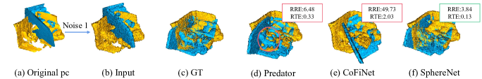
Figure 9: Qualitative results on the 3DMatch-noise benchmark. Our method achieves correct registration with the lowest RRE and RTE.

TABLE VI: Registration results on KITTI odometry.

Method	RTE(cm)	RRE(∘)	RR(%)
3DFeat-Net [51]	25.9	0.25	96.0
Predator [23]	6.8	0.27	99.8
CoFiNet [53]	8.2	0.41	99.8
GeoTransformer [36]	7.4	0.27	99.8
SphereNet (ours)	6.8	0.31	99.8

IV-C Evaluation on KITTI

Dataset and Metrics.   Following [4, 8, 23, 3], we used sequences 0-5 for training, sequences 6-7 for validation, and sequences 8-10 for testing. Since the ground truth transformation $\mathbf{T}\{\mathbf{R},\mathbf{t}\}$ raised by the authors is not accurate, we follow [4, 8] to use the iterative closest point (ICP) [5] algorithm to refine the ground truth transformation $\mathbf{T}$.

Following previous works [23, 3], we evaluate our SphereNet by three metrics: Relative Rotation Error (RRE), Relative Translation Error (RTE), and Success Rate (SR).

Relative Rotation Error, the geodesic distance between estimated and ground-truth rotation matrices, can be used to measure the error between our predicted rotation transformation and the ground-truth rotation transformation:

$$\mathrm{RRE}=\arccos\left(\frac{\operatorname{trace}\left(\hat{\mathbf{R}}_{h}^{T}\mathbf{R}_{h}\right)-1}{2}\right)$$ (23)

where $\hat{\mathbf{R}}_{h}$ and $\mathbf{R}_{h}$ are our predicted rotation matrix and the ground-truth rotation matrix respectively.

Relative Translation Error, the Euclidean distance between the estimated and ground-truth translation vectors, can be used to measure the error between our predicted translation transformation and the ground-truth translation transformation:

$$\mathrm{RTE}=\left\|\hat{\mathbf{t}}_{h}-\mathbf{t}_{h}\right\|$$ (24)

where $\hat{\mathbf{h}}_{t}$ and $\mathbf{h}_{t}$ are our predicted translation vector and the ground-truth translation vector respectively.

Success Rate is the ratio of the number of registration that errors within certain thresholds, which determines whether the registration is successful on KITTI. If the RRE is less than $2$m and the RTE is less than $5^{\circ}$, the registration on this point cloud pair is considered a successful registration.

$$\mathrm{SR}=\frac{1}{H}\sum_{h=1}^{H}\mathbbm{1}\left(\mathrm{RRE}_{h}<2\mathrm{~{}m}\wedge\mathrm{RTE}_{h}<5^{\circ}\right)$$ (25)

Registration Results.   We compare our SphereNet with strong baselines [51, 23, 53, 36] on RTE, RRE and SR. As shown in Table VI and Figure 12, our method achieves the highest SR and lowest RTE on KITTI, which means that our method is also competitive on outdoor datasets.

IV-D 3DMatch-noise: Robustness to Strong Noise

From the registration results, it can be seen that the most recent methods have determined good effects on the 3DMatch dataset, and the improvement is close to saturation. Therefore, a more challenging benchmark needs to be set. By adding high-intensity noises to the 3DMatch dataset, we construct a 3DMatch-noise benchmark to simulate the uncertainty of the real scenes and the imprecision of the sensors. Our high-intensity noises can be divided into four categories. The first category is a Gaussian noise $N(0,0.05^{2})$ (clipped to [-0.05, 0.05]), which is shown in Figure 7 (b). The second category shown in Figure 7 (c) is a noise subject to the uniform distribution $U(-0.05,0.05)$. As shown in Figure 7 (d), the third category is to randomly replace 5% of the original points with random numbers that obey the normal distribution $N(0,0.5^{2})$. For the fourth category, considering that 3DMatch is collected by using an RGB-D sensor, so it makes more sense to introduce noise from the depth map [31]. On the original depth map of 3DMatch, a residual that obeys Gaussian distribution $N(0,0.05^{2})$ is added to the depth channel of the depth map to generate a point cloud with Noise 4 [31].

We experiment on the 3DMatch-noise benchmark to further highlight the anti-noise ability of our SphereNet in the face of scenes with high-intensity noise. As shown in the Table V, compared with the state-of-the-arts [23, 53, 36, 30], in the scenes with strong noise, our method has a huge improvement over IR, FMR, and RR. Although our SphereNet doesn’t use noise augmentation such as [23, 53, 36, 30], it still achieves the best performances in four different types of noises, improving RR by 23.2 pp and FMR by 30.5 pp over the state-of-the-art method [36] on Noise 1. Moreover, after adding Noise 1, Noise 2, Noise 3, Noise 4 to 3DMatch, the RR obtained by our SphereNet only drops by 8.5 pp, 11.8 pp, 1.1 pp and 5.9 pp, while 38.3 pp, 31.0 pp, 5.8 pp and 26.9 pp for [36]. This highlights that our SphereNet has good robustness to strong noise and it also maintains accurate registration even in bad scenes with noise. As the qualitative results are shown in Figure 9, our SphereNet achieves correct registration with the low RRE and RTE.

To verify the stability and influence under different noises with different intensities, we set more abundant experiments on the 3DMatch dataset with noise. It can be seen from Table VII that, within a certain range, our method has a certain adaptability to the noise of different intensities. With the increase in the proportion of Noise 3, FMR only decreases in a small range. With the proportion of noise up to 9%, our RR score is still 85.6%. In contrast, our sphere is more sensitive to Noise 1, and RR score is only 51.8 when STD is 0.07. But it is still much higher than other algorithms.

TABLE VII: Detailed results with different noise, where Noise Std is the standard deviation of Noise 1 and proportion is the ratio of the added noise points to the original point cloud in Noise 3.

Noise 1				Noise 3
Noise Std	FMR	IR	RR	Proportion	FMR	IR	RR
0.00	98.2	52.6	91.2	0%	98.2	52.6	91.2
0.01	95.8	43.4	86.7	3%	97.2	44.9	88.2
0.03	89.6	38.0	70.2	5%	96.7	43.2	88.2
0.05	85.5	32.2	66.4	7%	96.1	41.9	87.6
0.07	72.9	21.7	51.8	9%	95.9	41.0	85.6

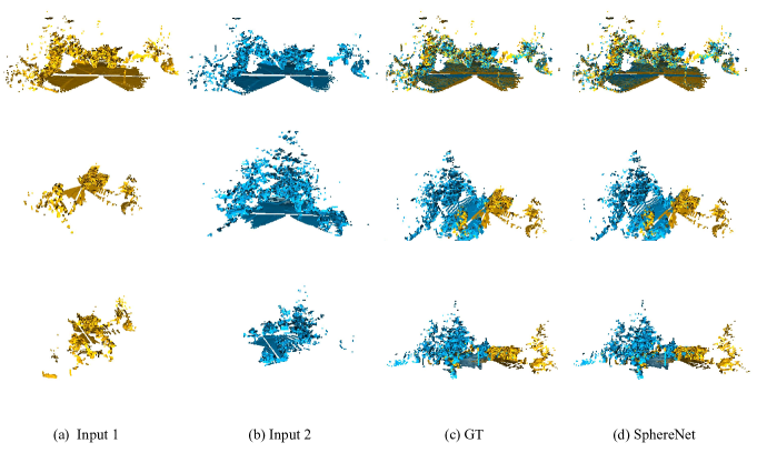
Figure 11: Registration results on the ETH dataset.

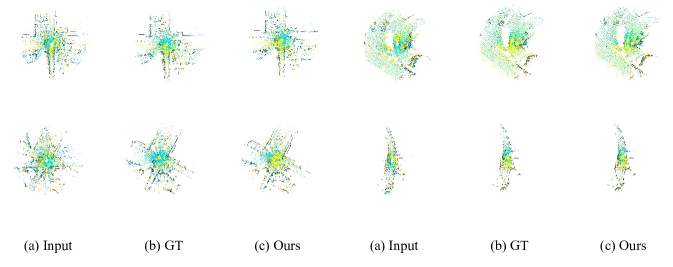
Figure 12: Registration results on the KITTI dataset.

IV-E Generalization across Different Datasets

Following [3, 4], we also evaluate the generalization ability of our SphereNet on the unseen datasets. In each experiment, our model is trained on one dataset, and multiscale feature fusion is used to overcome the differences in the scale between different datasets. Then, the trained model is directly tested on another dataset.

TABLE VIII: Results of generalization from 3DMatch to ETH.

	Gazebo		Wood		Avg.
	Summer	Winter	Autumn	Summer
FCGF [8]	22.8	10.0	14.8	16.8	16.1
D3Feat (rand) [4]	45.7	23.9	13.0	22.4	26.2
LMVD [29]	85.3	72.0	84.0	78.3	79.9
SpinNet [3]	92.9	91.7	92.2	94.4	92.8
GLORN [42]	90.3	91.6	78.5	83.2	85.9
SphereNet (ours)	94.6	95.8	92.2	93.6	94.5

Generalization from 3DMatch to ETH Dataset.   All our models are trained on the 3DMatch dataset and then tested on the ETH dataset with multiscale feature fusion. As shown in Table VIII and Figure 11, we achieve the best results in three different scenes, and the total average FMR reaches 94.53% which is close to 2 pp higher than the state-of-the-art [3].

TABLE IX: Results of generalization from KITTI to 3DMatch.

	RTE (cm)		RRE (∘)		Success (%)
	AVG	STD	AVG	STD
FCGF [8]	27.1	5.58	1.61	1.51	24.19
D3Feat-rand [4]	37.8	9.98	1.58	1.47	18.47
D3Feat-pred [4]	31.6	10.1	1.44	1.35	36.76
SpinNet [3]	15.6	1.89	0.98	0.63	81.44
SphereNet (ours)	9.9	0.71	0.57	0.33	87.20

Generalization from 3DMatch to KITTI Dataset.   Our models are trained on the 3DMatch dataset and then directly tested on the KITTI dataset. Similarly, it is difficult to generalize from 3DMatch to KITTI across different sensors. As shown in Table IX, the generalization ability of our method also shows the best performance on KITTI, achieving the minimum AVG and STD in RTE and RRE. And SR of the registration is also up to 87.20%, which is nearly 6 pp higher than the previous best method [3].

IV-F Running Times

TABLE X: Comparison of the running times.

Method	Samples	$t_{1}(s/pc)$	$t_{2}(s/pcp)$	$t_{total}(s/pcp)$
PerfectMatch[18]	5000	9.15	0.19	18.49
SpinNet[3]	5000	11.76	0.62	24.14
SphereNet (ours)	5000	3.90	0.61	8.41

Previous works [46, 53, 2] have shown that the speed of patch-based methods is much slower than that of fragment-based methods. Although our SphereNet has some disadvantages in running time, it has greatly improved in speed compared with previous patch-based methods [3, 18]. The running times of different stages are listed in Table X. As shown in Table X, compared with the previous patch-based methods, our method has a significant improvement. For completing the registration of one point cloud pair, the speed of our Sphere has improved by approximately 65% compared to SpinNet [3].

IV-G Ablation Study

In order to better evaluate the effectiveness of each module in our SphereNet, we conduct ablation experiments on 3DMatch and 3DMatch-noise. In the ablation experiment, we used three metrics FMR, IR, and RR to evaluate our results.

TABLE XI: Analysis experiments on 3DMatch / 3DMatch-noise / ETH. N, M, K: Number of spherical voxels in three dimensions. R: Radius of the descriptor. SV: Our spherical voxelization. SG: Spherical voxelization by sphere grouping. TI: Spherical interpolation. MSF: Multiscale feature fusion. SP: Spherical integrity padding. ZP: Zero padding. MLP: Use MLP for feature extraction. SCNN: Use SCNN for feature extraction.

No.	N	M	K	R	SV	SG	TI	MSF	SP	ZP	MLP	SCNN	3DMatch		3DMatch-noise		ETH
													FMR(%)	RR(%)	FMR(%)	RR(%)	FMR(%)
1)	15	20	40	0.3	✓		✓		✓			✓	98.2	91.2	77.7	53.8	94.5
2)	15	20	40	0.5	✓		✓		✓			✓	98.1	90.8	76.1	55.4	90.5
3)	15	20	40	1.0	✓		✓		✓			✓	98.0	90.2	74.6	55.1	41.6
4)	15	40	80	0.3	✓		✓		✓			✓	98.0	90.1	76.1	55.4	74.1
5)	15	20	40	0.3		✓			✓			✓	75.5	52.5	32.1	14.1	36.3
6)	15	20	40	0.3	✓				✓			✓	70.6	46.2	13.3	4.3	16.7
7)	15	20	40	0.3	✓		✓	✓	✓			✓	98.1	90.5	85.5	66.4	95.8
8)	15	20	40	0.3	✓		✓			✓		✓	95.2	84.9	72.6	52.5	74.3
9)	15	20	40	0.3	✓		✓		✓		✓		51.3	31.6	10.3	9.6	9.5

(1) Replacing the spherical voxelization with the sphere grouping.   Spherical voxelization can well capture the geometric feature from the perspective of geometric structure, and it can cooperate well with our spherical CNN. In this experiment, we replacing the spherical voxelization with the sphere grouping to form the initial feature by searching the nearest neighbors in the fixed position. By comparing the Row 1 and 5 in Table XI, without using the spherical voxelization to encode the initial feature, the ablated method has a lower FMR score than the complete method. And also, the performances on 3DMatch-noise and ETH significantly reduce. This illustrates that spherical voxelization is a great contribution to the finer geometric feature and better generalization ability.

(2) Only removing the spherical interpolation.   In order to ensure the fineness of the initial feature with less voxel grids, we introduce the spherical interpolation, which can improve the robustness against noise. In this experiment, we remove the spherical interpolation and directly use the initial feature generated by spherical voxelization to extract the descriptor. As shown in Row 1 and 6, without using the spherical interpolation, the ablated method performs poorly on the 3DMatch-Noise benchmark and ETH dataset. This shows that our spherical interpolation can greatly improve the anti-noise ability and generalization ability.

(3) Only replacing the spherical integrity padding with zero padding.   Due to the particularity of our spherical voxelization, the obtained initial feature has some certain loss on the boundaries, and our spherical integrity padding can solve this problem well. In this experiment, we replace the spherical integrity padding with zero padding. By comparing the Row 1 and 8 in Table XI, the method with spherical integrity padding has improved RR from 84.9% to 91.2%, which important to improve the performance of our method. In addition, it also has a contribution to anti-noise ability.

(4) Only replacing the spherical CNN with MLPs.   Our spherical CNN can cooperate with the spherical voxelization to complete the extraction of rotation-invariant and robust descriptors. In this experiment, only MLP is used instead of spherical CNN to verify the significant improvement of our spherical CNN for registration. As shown in Row 1 and 9, without spherical CNN, the ablated method cannot achieve accurate feature matching and registration, which shows that our spherical CNN are crucial for this robust descriptor extraction.

(5) Only removing the Multiscale Feature Fusion.   Our MSF module introduces a scale channel and refines the initial features without new overhead to further improve the generalization ability and anti-noise ability. As can be seen from Row 1 and 7 of Table XI, our method with MSF module achieves a 1.3% improvement in RR on the ETH dataset and a 12.6% improvement on the 3DMatch-noise benchmark.

Why does the model have better generalization?

First, MSF module. Comparing Row 1 and 7 in Table XI, The generalization performance is improved by using MSF module. Although the generalization performance of the local context [3] is excellent, we still achieve better results than SpinNet [3] by our MSF module. It is difficult in unseen datasets because of the inconsistent scale and sparsity. So a suitable radius of the descriptor is necessary to focus on the local area, such as “a chair” in 3DMatch or “a vehicle” in KITTI which is more distinctive for matching. SpinNet [3] only adjusts the radius of the descriptor manually which has a limited effect. This paper proposes the MSF module, which divides a local sphere into multiscale spheres, then carries out feature fusion. In this way, the “suitable area” can be better captured, which greatly improves the generalization ability.

Second, spherical voxelization. Comparing the results of the first and fifth rows in Table XI, it can be seen that our spherical interpolation method has greatly contributed to the improvement of generalization ability. This is because, different from SG method (Row 5) in SpinNet [3], the area size of our generated voxels is regular and proportional to the descriptor radius $R$ of our method. Therefore, our SV method can adapt the size of a small voxel according to the descriptor radius $R$, which can better improve the adaptability of our method to the scale inconsistency of different datasets. However, SG method uses the neighbor search with a fixed radius to generate small voxels, which can’t adapt to the scale inconsistency of different datasets well.

Why does the model have anti-noise ability?

First, spherical voxelization. As shown in Row 1 and 5 on Table XI, Our method on spherical voxelization has a better contribution on anti-noise ability than method in SpinNet [3]. Analyzing the cause, SpinNet [3] builds the voxels by performing radius neighbor search at fixed locations and setting the number of voxel grids to 9*40*80, which leads to a high overlap of the regions where point-based layers are performed. So a small amount of noise will affect more histogram bins. In our method, the sphere is strictly divided into voxels in three directions, and the number of voxels is fewer. There is no overlapping area in the histogram generation. So the noise will only affect fewer histogram bins.

Second, spherical interpolation. Comparing Row 1 and 6 in Table XI, using TI achieves a great improvement on RR and without it RR is only 4.3%. Therefore, our TI has a good contribution to the improvement of anti-noise ability. As we describe in Section III-B, a point is interpolated to the 8 surrounding voxels, rather than voting completely to a voxel. many points affected by noise will be offset from the position $\mathbf{p}_{i_{j}}\in\mathbf{V}_{n_{1}m_{1}k_{1}}$ to $\mathbf{p}_{i_{j}}+\boldsymbol{\varepsilon}\in\mathbf{V}_{n_{2}m_{2}k_{2}}$. When the noise intensity is within a certain range, both $\mathbf{V}_{n_{1}m_{1}k_{1}}$ and $\mathbf{V}_{n_{2}m_{2}k_{2}}$ belong to the 8 surrounding voxels. Therefore, our spherical interpolation can weaken the effect of noise on the initial features.

V Conclusion

We propose SphereNet to learn a noise-robust and unseen-general descriptor for point cloud registration. We encode the initial geometric feature by spherical voxelization with spherical interpolation so that we can fully capture the geometric features. After that, descriptors are extracted by spherical CNN with spherical integrity padding, which makes the descriptors more robust and general. Thanks to these methods, SphereNet achieves the state-of-the-art performance compared with other learning-based methods. In addition, it also achieves the best anti-noise ability on the noisy scenes and generalization performance on the unseen scenes. In the future, by the research of new technologies, we will use SphereNet framework to complete the task of non-rigid point cloud registration.

References

- [1] Aitor Aldoma, Federico Tombari, Radu Bogdan Rusu, and Markus Vincze. Our-cvfh–oriented, unique and repeatable clustered viewpoint feature histogram for object recognition and 6dof pose estimation. In Joint DAGM (German Association for Pattern Recognition) and OAGM Symposium, pages 113–122. Springer, 2012.
- [2] Sheng Ao, Yulan Guo, Qingyong Hu, Bo Yang, Andrew Markham, and Zengping Chen. You only train once: Learning general and distinctive 3d local descriptors. IEEE Transactions on Pattern Analysis and Machine Intelligence, 45(3):3949–3967, 2023.
- [3] Sheng Ao, Qingyong Hu, Bo Yang, Andrew Markham, and Yulan Guo. Spinnet: Learning a general surface descriptor for 3d point cloud registration. In Proceedings of the IEEE/CVF Conference on Computer Vision and Pattern Recognition, pages 11753–11762, 2021.
- [4] Xuyang Bai, Zixin Luo, Lei Zhou, Hongbo Fu, Long Quan, and Chiew-Lan Tai. D3feat: Joint learning of dense detection and description of 3d local features. In Proceedings of the IEEE/CVF conference on computer vision and pattern recognition, pages 6359–6367, 2020.
- [5] Paul J Besl and Neil D McKay. Method for registration of 3-d shapes. In Sensor fusion IV: control paradigms and data structures, volume 1611, pages 586–606. Spie, 1992.
- [6] Zhi Chen, Kun Sun, Fan Yang, and Wenbing Tao. Sc2-pcr: A second order spatial compatibility for efficient and robust point cloud registration. In Proceedings of the IEEE/CVF Conference on Computer Vision and Pattern Recognition, pages 13221–13231, 2022.
- [7] Christopher Choy, JunYoung Gwak, and Silvio Savarese. 4d spatio-temporal convnets: Minkowski convolutional neural networks. In Proceedings of the IEEE/CVF Conference on Computer Vision and Pattern Recognition, pages 3075–3084, 2019.
- [8] Christopher Choy, Jaesik Park, and Vladlen Koltun. Fully convolutional geometric features. In 2019 IEEE/CVF International Conference on Computer Vision (ICCV), pages 8957–8965, 2019.
- [9] Chin Seng Chua and Ray Jarvis. Point signatures: A new representation for 3d object recognition. International Journal of Computer Vision, 25(1):63–85, 1997.
- [10] Taco S Cohen, Mario Geiger, Jonas Köhler, and Max Welling. Spherical cnns. arXiv preprint arXiv:1801.10130, 2018.
- [11] Haowen Deng, Tolga Birdal, and Slobodan Ilic. Ppf-foldnet: Unsupervised learning of rotation invariant 3d local descriptors. In Proceedings of the European Conference on Computer Vision (ECCV), pages 602–618, 2018.
- [12] Haowen Deng, Tolga Birdal, and Slobodan Ilic. Ppfnet: Global context aware local features for robust 3d point matching. In Proceedings of the IEEE conference on computer vision and pattern recognition, pages 195–205, 2018.
- [13] Joao Paulo Silva do Monte Lima and Veronica Teichrieb. An efficient global point cloud descriptor for object recognition and pose estimation. In 2016 29th SIBGRAPI conference on graphics, patterns and images (SIBGRAPI), pages 56–63. IEEE, 2016.
- [14] Bertram Drost, Markus Ulrich, Nassir Navab, and Slobodan Ilic. Model globally, match locally: Efficient and robust 3d object recognition. In 2010 IEEE computer society conference on computer vision and pattern recognition, pages 998–1005. Ieee, 2010.
- [15] Carlos Esteves, Christine Allen-Blanchette, Ameesh Makadia, and Kostas Daniilidis. Learning so (3) equivariant representations with spherical cnns. In Proceedings of the European Conference on Computer Vision (ECCV), pages 52–68, 2018.
- [16] Andrea Frome, Daniel Huber, Ravi Kolluri, Thomas Bülow, and Jitendra Malik. Recognizing objects in range data using regional point descriptors. In European conference on computer vision, pages 224–237. Springer, 2004.
- [17] Andreas Geiger, Philip Lenz, and Raquel Urtasun. Are we ready for autonomous driving? the kitti vision benchmark suite. In 2012 IEEE conference on computer vision and pattern recognition, pages 3354–3361. IEEE, 2012.
- [18] Zan Gojcic, Caifa Zhou, Jan D. Wegner, and Andreas Wieser. The perfect match: 3d point cloud matching with smoothed densities. In 2019 IEEE/CVF Conference on Computer Vision and Pattern Recognition (CVPR), pages 5540–5549, 2019.
- [19] Yulan Guo, Mohammed Bennamoun, Ferdous Sohel, Min Lu, Jianwei Wan, and Ngai Ming Kwok. A comprehensive performance evaluation of 3d local feature descriptors. International Journal of Computer Vision, 116(1):66–89, 2016.
- [20] Yulan Guo, Ferdous Sohel, Mohammed Bennamoun, Min Lu, and Jianwei Wan. Rotational projection statistics for 3d local surface description and object recognition. International journal of computer vision, 105(1):63–86, 2013.
- [21] Kaiming He, Xiangyu Zhang, Shaoqing Ren, and Jian Sun. Deep residual learning for image recognition. In Proceedings of the IEEE conference on computer vision and pattern recognition, pages 770–778, 2016.
- [22] Bo Hu, Shenglong Zhou, Zhiwei Xiong, and Feng Wu. Cross-resolution distillation for efficient 3d medical image registration. IEEE Transactions on Circuits and Systems for Video Technology, 32(10):7269–7283, 2022.
- [23] Shengyu Huang, Zan Gojcic, Mikhail Usvyatsov, Andreas Wieser, and Konrad Schindler. Predator: Registration of 3d point clouds with low overlap. In Proceedings of the IEEE/CVF Conference on computer vision and pattern recognition, pages 4267–4276, 2021.
- [24] Xiaoshui Huang, Guofeng Mei, Jian Zhang, and Rana Abbas. A comprehensive survey on point cloud registration. arXiv preprint arXiv:2103.02690, 2021.
- [25] Xiaoshui Huang, Jian Zhang, Qiang Wu, Lixin Fan, and Chun Yuan. A coarse-to-fine algorithm for matching and registration in 3d cross-source point clouds. IEEE Transactions on Circuits and Systems for Video Technology, 28(10):2965–2977, 2017.
- [26] Chiyu Jiang, Jingwei Huang, Karthik Kashinath, Philip Marcus, Matthias Niessner, et al. Spherical cnns on unstructured grids. arXiv preprint arXiv:1901.02039, 2019.
- [27] Andrew E Johnson and Martial Hebert. Using spin images for efficient object recognition in cluttered 3d scenes. IEEE Transactions on pattern analysis and machine intelligence, 21(5):433–449, 1999.
- [28] Huan Lei, Naveed Akhtar, and Ajmal Mian. Octree guided cnn with spherical kernels for 3d point clouds. In Proceedings of the IEEE/CVF Conference on Computer Vision and Pattern Recognition, pages 9631–9640, 2019.
- [29] Lei Li, Siyu Zhu, Hongbo Fu, Ping Tan, and Chiew-Lan Tai. End-to-end learning local multi-view descriptors for 3d point clouds. In Proceedings of the IEEE/CVF Conference on Computer Vision and Pattern Recognition, pages 1919–1928, 2020.
- [30] Yang Li and Tatsuya Harada. Lepard: Learning partial point cloud matching in rigid and deformable scenes. In Proceedings of the IEEE/CVF Conference on Computer Vision and Pattern Recognition, pages 5554–5564, 2022.
- [31] Tanwi Mallick, Partha Pratim Das, and Arun Kumar Majumdar. Characterizations of noise in kinect depth images: A review. IEEE Sensors journal, 14(6):1731–1740, 2014.
- [32] Anastasiia Mishchuk, Dmytro Mishkin, Filip Radenovic, and Jiri Matas. Working hard to know your neighbor’s margins: Local descriptor learning loss. Advances in neural information processing systems, 30, 2017.
- [33] François Pomerleau, Ming Liu, Francis Colas, and Roland Siegwart. Challenging data sets for point cloud registration algorithms. The International Journal of Robotics Research, 31(14):1705–1711, 2012.
- [34] Charles R Qi, Hao Su, Kaichun Mo, and Leonidas J Guibas. Pointnet: Deep learning on point sets for 3d classification and segmentation. In Proceedings of the IEEE conference on computer vision and pattern recognition, pages 652–660, 2017.
- [35] Charles Ruizhongtai Qi, Li Yi, Hao Su, and Leonidas J Guibas. Pointnet++: Deep hierarchical feature learning on point sets in a metric space. Advances in neural information processing systems, 30, 2017.
- [36] Zheng Qin, Hao Yu, Changjian Wang, Yulan Guo, Yuxing Peng, and Kai Xu. Geometric transformer for fast and robust point cloud registration. In Proceedings of the IEEE/CVF Conference on Computer Vision and Pattern Recognition, pages 11143–11152, 2022.
- [37] Olaf Ronneberger, Philipp Fischer, and Thomas Brox. U-net: Convolutional networks for biomedical image segmentation. In International Conference on Medical image computing and computer-assisted intervention, pages 234–241. Springer, 2015.
- [38] Radu Bogdan Rusu, Nico Blodow, and Michael Beetz. Fast point feature histograms (fpfh) for 3d registration. In 2009 IEEE International Conference on Robotics and Automation, pages 3212–3217, 2009.
- [39] Radu Bogdan Rusu, Nico Blodow, Zoltan Csaba Marton, and Michael Beetz. Aligning point cloud views using persistent feature histograms. In 2008 IEEE/RSJ International Conference on Intelligent Robots and Systems, pages 3384–3391, 2008.
- [40] Radu Bogdan Rusu, Gary Bradski, Romain Thibaux, and John Hsu. Fast 3d recognition and pose using the viewpoint feature histogram. In 2010 IEEE/RSJ International Conference on Intelligent Robots and Systems, pages 2155–2162, 2010.
- [41] Samuele Salti, Federico Tombari, and Luigi Di Stefano. Shot: Unique signatures of histograms for surface and texture description. Computer Vision and Image Understanding, 125:251–264, 2014.
- [42] Jules Sanchez, Jean-Emmanuel Deschaud, and Francois Goulette. Domain generalization of 3d semantic segmentation in autonomous driving. arXiv preprint arXiv:2212.04245, 2022.
- [43] Hugues Thomas, Charles R Qi, Jean-Emmanuel Deschaud, Beatriz Marcotegui, François Goulette, and Leonidas J Guibas. Kpconv: Flexible and deformable convolution for point clouds. In Proceedings of the IEEE/CVF international conference on computer vision, pages 6411–6420, 2019.
- [44] Ashish Vaswani, Noam Shazeer, Niki Parmar, Jakob Uszkoreit, Llion Jones, Aidan N Gomez, Łukasz Kaiser, and Illia Polosukhin. Attention is all you need. Advances in neural information processing systems, 30, 2017.
- [45] Athanasios Voulodimos, Nikolaos Doulamis, Anastasios Doulamis, and Eftychios Protopapadakis. Deep learning for computer vision: A brief review. Computational intelligence and neuroscience, 2018, 2018.
- [46] Haiping Wang, Yuan Liu, Zhen Dong, and Wenping Wang. You only hypothesize once: Point cloud registration with rotation-equivariant descriptors. In Proceedings of the 30th ACM International Conference on Multimedia, pages 1630–1641, 2022.
- [47] Yue Wu, Xidao Hu, Yue Zhang, Maoguo Gong, Wenping Ma, and Qiguang Miao. Sacf-net: Skip-attention based correspondence filtering network for point cloud registration. IEEE Transactions on Circuits and Systems for Video Technology, 2023.
- [48] Yue Wu, Yue Zhang, Xiaolong Fan, Maoguo Gong, Qiguang Miao, and Wenping Ma. Inenet: Inliers estimation network with similarity learning for partial overlapping registration. IEEE Transactions on Circuits and Systems for Video Technology, 2022.
- [49] Fan Yang, Lin Guo, Zhi Chen, and Wenbing Tao. One-inlier is first: Towards efficient position encoding for point cloud registration. Advances in Neural Information Processing Systems, 35:6982–6995, 2022.
- [50] Jiaqi Yang, Zhiqiang Huang, Siwen Quan, Qian Zhang, Yanning Zhang, and Zhiguo Cao. Toward efficient and robust metrics for ransac hypotheses and 3d rigid registration. IEEE Transactions on Circuits and Systems for Video Technology, 32(2):893–906, 2021.
- [51] Zi Jian Yew and Gim Hee Lee. 3dfeat-net: Weakly supervised local 3d features for point cloud registration. In Proceedings of the European conference on computer vision (ECCV), pages 607–623, 2018.
- [52] Hao Yu, Ji Hou, Zheng Qin, Mahdi Saleh, Ivan Shugurov, Kai Wang, Benjamin Busam, and Slobodan Ilic. Riga: Rotation-invariant and globally-aware descriptors for point cloud registration. arXiv preprint arXiv:2209.13252, 2022.
- [53] Hao Yu, Fu Li, Mahdi Saleh, Benjamin Busam, and Slobodan Ilic. Cofinet: Reliable coarse-to-fine correspondences for robust pointcloud registration. Advances in Neural Information Processing Systems, 34:23872–23884, 2021.
- [54] Andy Zeng, Shuran Song, Matthias Nießner, Matthew Fisher, Jianxiong Xiao, and Thomas Funkhouser. 3dmatch: Learning local geometric descriptors from rgb-d reconstructions. In Proceedings of the IEEE conference on computer vision and pattern recognition, pages 1802–1811, 2017.
- [55] Zhiyuan Zhang, Jiadai Sun, Yuchao Dai, Bin Fan, and Mingyi He. Vrnet: Learning the rectified virtual corresponding points for 3d point cloud registration. IEEE Transactions on Circuits and Systems for Video Technology, 32(8):4997–5010, 2022.
- [56] Guiyu Zhao, Hongbin Ma, and Ying Jin. A method for robust object recognition and pose estimation of rigid body based on point cloud. In International Conference on Intelligent Robotics and Applications, pages 468–480. Springer, 2022.