What is a reference frame in General Relativity?

Abstract

In General Relativity, the terms ‘reference frame’ and ‘coordinate system’ must be distinguished. The former refers to physical systems that are dynamically coupled with the gravitational field, aside from possible approximations, while the latter refers to a set of mathematical variables that are representative artefacts. This necessary distinction is lost in pre-general relativistic physics, where we can choose as a reference frame a system of real physical objects that is not affected and cannot affect the physical system under consideration. Therefore, we can make it coincide with a coordinate system without the need for approximations. We propose a a novel three-fold distinction between three types of reference frames, considered as material systems. In particular, we discern between Idealised Reference Frames, Dynamical Reference Frames and Real Reference Frames, depending on their increasing physical role in the total dynamics. Using a Bianchi I model in Minisuperspace, we give a cosmological example of the use of a gravitational Dynamical Reference Frame, namely a reference frame constructed with gravitational degrees of freedom in the standard case where the gravitational stress-energy tensor is not defined in the Einstein field equations. We also analyse the role of active and passive diffeomorphisms in changing a reference frame.

1 Introduction

In the ‘post-Einsteinian’ physical and philosophical literature, due to some ambiguity which can be traced back to Einstein himself, it has been customary to conflate the terms ‘reference frame’ and ‘coordinate system’, which have been used somewhat interchangeably, or at least have not been always clearly distinguished. To give just an example, in [Bergmann(1962), p.207]) the author states:

In all that follows we shall use the terms ‘curvilinear four-dimensional coordinate system’ and ‘frame of reference’ interchangeably.

This problem has been egregiously highlighted in its philosophical-historical components and addressed in [Norton(1989)] and [Norton(1993)]. In the present paper, we claim that the issue is still open: the two terms have still not been properly differentiated yet. We believe that our contribution is relevant because there is no discussion of the differences between the two concepts in the recent literature. To date, to the best of our knowledge, the works that deal most with this issue are those of Norton mentioned above (see also [Norton(1985)]). The purpose of this paper is to clarify the nature of a reference frame in General Relativity (GR), by first proposing a criterion to distinguish it from a set of coordinates and then classifying three ways to understand the notion of a reference frame in GR, considered as a material system [Rovelli(1991a)]. The benefit of this constraint is essentially due to the fact that GR is only deparametrizable for some specific material models. For such models, one is able to derive gauge-invariant Dirac observables, i.e., quantities invariant under the gauge group of the theory. In particular, we call Idealised Reference Frames (IRFs) those physical systems where both the dynamical equations and the stress-energy contribution to the Einstein Field Equations (EFEs) are neglected. The second class is that of Dynamical Reference Frames (DRFs), whose back-reaction on the spacetime metric is neglected, but the frame satisfies a specific dynamical equation. Finally, we name Real Reference Frames (RRFs) those ones whose stress-energy contribution to the EFEs is taken into account, as well as their dynamics. Although RRFs are systems of great interest, as they are physically more realistic in principle, in the remainder of the paper we deal exclusively with IRFs and DRFs.

Before proceeding, a clarification on the choice of nomenclature is worthwhile. There is a tendency in the literature to conflate two distinct things, namely, ‘idealisation’ and ‘approximation’ [Norton(2012)]. In the correct characterisation, ‘idealisation’ means the way to replace a target system under study with a distinct fictitious novel system whose properties provide an inexact description of some aspects of the target system. ‘Approximation’ means the way to treat certain quantities of the target system as negligible compared to others. Namely, it is an inexact description of the target system. The crucial difference, then, lies in whether one introduces a novel system. Here, we understand IRFs (as well as DRFs) as approximations, not idealisations. In that, as we shall see in more detail, we proceed with approximations to a non-approximated reference frame target system, which we shall designate by the name of RRF. However, to be fair, RRFs are divided into a subclass that conceals an approximation to a real physical system in the strict sense of the term, understood as a target reference frame where no approximation is implemented.

The proposed classification allow us to find a possible reason why the notions of reference frame and coordinate system are usually conflated in GR. According to us, the confusion stems from the practical, but not conceptual, equivalence that exists between IRFs and coordinate systems. Furthermore, we propose a formal argument to distinguish between DRFs and coordinates. Specifically, we posit that we can switch between two DRFs through a transformation linking two different gauge choices and this amount to use an active diffeomorphism. On the other hand, coordinates are related by passive diffeomorphisms.

Using a very simple cosmological example, namely a Bianchi I Minisuperspace model [Bianchi(1989)] with two equal scale factors, we introduce a class of DRFs, which we name ‘gravitational dynamical reference frame’, or gDRFs. A gDRF is represented by gravitational degrees of freedom, in the standard case where the gravitational stress-energy tensor is not defined in the EFEs. Early attempts to use purely gravitational degrees of freedom as a reference frame were proposed by Bergmann and Komar in ([Bergmann(1961a)],[Bergmann(1961b)],[Bergmann and Komar(1960)],[Komar(1958)]), who constructed space-time scalars from gravitational degrees of freedom that serve as dynamically coupled reference frames and as ‘locators’ for points. Our example is interesting because it may open the way for future work on characterising reference frames consisting of gravitational and non-material degrees of freedom in the case of pure vacuum GR. Such work, however, will not be carried out in this paper. For the purpose of our discussion, the role of the Bianchi I model will be twofold. Firstly, it will allow us to introduce a general-relativistic case in which a change of a DRF is implemented by an active diffeomorphism. Secondly, it will also clarify in what sense a passive diffeomorphism can implement a change of DRF. To this end, the distinction between gDRF and DRF is superfluous, although conceptually important and rightly worth exploring. The most relevant application of the Minisuperspace framework corresponds to the case of a homogeneous Universe, which is described by a class of cosmologies known as Bianchi models. The construction of the Hamiltonian representation of Bianchi models dynamics is usually performed by using a set of variables known as Misner variables $(\alpha,\beta_{\pm})$ [Misner(1969)]. In particular, the variable $\alpha$ is related to the volume of the Universe, which scales as $e^{3\alpha/2}$. The variables $\beta_{\pm}$ represent the spatial anisotropies and correspond to the two physical degrees of freedom of gravity.

This paper clarifies the nature of an important and ubiquitous concept in physics: that of reference frame. In fact, whenever we set up an experiment or formalise the behaviour of a physical system, we implicitly or explicitly use a reference frame. The main question of the present work is what a reference frame in GR is. One reason why it is important to reach this end is that researchers in contemporary physics and philosophy of physics are interested in quantum reference (see [Rovelli(1991b)], [Giacomini et al.(2019)], [Hoehn and Vanrietvelde(2020)]). In fact, all physical systems are, to our knowledge, ultimately quantum. We argue that, before we can really have a discussion on quantum reference frames in quantum gravity, we should know properly what reference frames are in classical GR.

The paper is structured as follows.

In Section 2, we analyse the role of reference frames in General Relativity and pre-general relativistic physics.

Section 3 contains the detailed classification of three possible ways of understanding a reference frame, supported by some concrete examples.

In Section 4, we provide some examples that demonstrate the origin of the confusion between the notions of reference frame and coordinate system in GR.

In Section 5, we analyse the definition of reference frame as provided by Earman and Norton. We then compare this class of reference frames with the Brown-Kuchař dust.

In section 6 we develop an argument with the aim of distinguishing between a DRF and a coordinate system, based on the different kind of map that implements a DRF and a coordinate change, respectively. By introducing a simplified Bianchi I model (6.1), we also give a cosmological example of a gDRF. This will shed more light on the differences between DRFs and coordinate systems.

2 Reference Frames vs. Coordinate systems: ‘three decades of (missing) dispute’

After Norton and Earman’s analysis of the concepts of coordinate system and reference frame between the 1970s and 1990s, it has become common practice within the literature to consider this conceptual problem solved. However, we argue that it is necessary to revive the debate and recognise its specific relevance within the analysis of the foundations of GR. The main motivations, which will be analysed below, concern the physical interpretation of gauge freedom, as well as interpretation of vacuum GR (Section 3); the fictitious role of coordinates in GR and the exposition of a new perspective on why the two concepts are often used interchangeably without much care (Section 4).

The conventional informal way to distinguish the concept of reference frame from that of coordinate system is to point out that only a reference frame has a link to an observer’s state of motion ([DiSalle(2020)], see also [Pooley(2017)]). Following the work of Earman (in particular [Earman(1974)]) and Norton, the modern literature dealing with spatiotemporal theories in the broadest sense formally associates to a reference frame a timelike four-velocity field on a manifold (see e.g. [Bradley(2021)]). Equivalently a reference frame is defined as a congruence of worldlines in space-time characterising the state of motion of a physical system. We will show that these kinds of definitions do not fully exhaust the characterisation of reference frames. On the other hand, some ambiguity still appears in [Read(2020)], in which the two terms are not clearly differentiated. In fact, on page 215 a (reference) frame-dependent object is defined as a ‘non-tensorial object’, that is thought of as a ‘coordinate-dependent object’ (ivi, p. 217).

The need to separate the two concepts does not emerge in pre-general relativistic (pre-GR) physics, since a reference frame can be represented as a set of degrees of freedom ‘provided from outside’ [Henneaux and Teitelboim(1994)]. For example, within Maxwell’s theory in Minkowskian spacetime, the Maxwell field is understood as a subsystem of the Universe that does not affect the global inertial reference frame that can be defined on the fixed background structure. For instance, we can define locations in spacetime by means of non electrically charged objects, which constitute the reference frame. This point is elucidated in the following passage in [Einstein(1905), p.38]:

The theory to be developed—like every other electrodynamics—is based upon the kinematics of rigid bodies, since the assertions of any such theory concern relations between rigid bodies (systems of coordinates), clocks, and electromagnetic processes.

This passage can be interpreted to mean that the special relativistic theory is concerned with the relations between electromagnetic processes and material bodies that are ‘dynamically external’ to the electromagnetic system under study, which Einstein calls ‘system of coordinates’.

In contrast, GR has no available ‘outside’. Namely, to be rigorous, we should not be allowed to consider reference frames as dynamically external, as we do in pre-GR physics. This follows from the fact that no existing physical system is gravitationally neutral. In other words, there is no way to disregard the interaction between the gravitational field and the reference objects. As we shall see, the fact that we cannot disregard the interaction between the gravitational field and the reference frame is true, unless approximations are made to the system constituting the reference frame itself. But it is precisely here that the lines become blurry. In pre-GR physics there is no need for approximations: it is always possible to define a reference frame as s physically ‘irrelevant’ real system and to make it coincide with the notion of coordinate system. In contrast, in GR the only physically significant way to introduce a physical coordination is to have it substantiated by a gravitationally interacting system. Therefore, the concept of a coordinate system, even if is widely used throughout the general relativistic literature, should be considered as a representational artefact without a physical interpretation. By this, we mean that in pre-GR physics a coordinate system may correspond to a system of physical objects external to the dynamics of the problem, but in GR a coordinate system has no underlying physical content. In other words, it has no a direct physical referent. If this were not the case, it would be a set of gravitationally charged degrees of freedom and thus not dynamically ‘external’. Consequently, in GR a reference frame cannot be understood as equivalent to a set of non-dynamic spacetime coordinates. As we shall see, the only way to make the reference frame ‘dynamically external’ is to implement approximations. So, it is clear that, conceptually, the notions of reference frame and coordinate system do not naturally coincide in GR.

Having clarified the physical status of reference frames, however, it is still necessary to define their nature. What is a reference frame? Let us summarise the main definitions of reference frame that can be found in the literature, from which all others are derived. The one that best meets the emphasised necessary distinction between the two concepts in GR is found in [Rovelli(1991a)]. Here, the most basic way to introduce a reference frame is to define it as a set of variables representing a material system, for example a set of physical bodies or a matter field, such that these degrees of freedom can be used to define a spatiotemporal location in the relational sense. This definition will ground our classification in Section 3. From [Rovelli(1991a)] also comes the suggestion that in GR reference frames can be considered dynamically external only if they are approximated. Moreover, as we already said, in the above-mentioned work of Norton and Earman (see also [Earman and Glymour(1978)]), as is now common in the vast majority of the physical and philosophical literature of GR, a reference frame is defined by a smooth, timelike four-velocity vector field $U^{a}$ tangent to the worldlines of a material system to which an equivalence class of coordinates is locally adapted (see also[Brown(2005)]). We will see more details in Section 5. It is straightforward that to consider the physical relevance of this definition of a reference frame, the vector field, exemplified e.g. by massive particle worldlines, should take into account the coupled dynamics between the particle system and the gravitational degrees of freedom. On the contrary, the vector field is usually treated as not fully coupled with gravitational dynamics.

3 IRF, DRF, RRF

In this section and throughout the paper, following [Rovelli(1991a)] and [Rovelli(2004)], we define a reference frame at the most basic level as a gravitationally interacting material system. We argue that in GR we can mean three different things by the term ‘reference frame’. This novel three-fold division is based on the degree of approximation applied to a material system, which makes its dynamics more or less intertwined with that of the gravitational field. Although the paper follows the reasoning presented in [Rovelli(1991a)] that adopting approximations in defining a reference frame will blur its physical significance, while reconsidering its stress-energy presence and the dynamics will bring the physical significance back into focus, our proposal provides an independent contribution to this topic. In particular, the work makes a new contribution in that it complements previous work, incorporates additional tools and engages with more philosophical literature Rovelli’s original proposal. To give a concrete example, in [Rovelli(1991a)] the author completely ignores the class of DRFs, which are dealt with extensively here. This fact is curious because, as we shall see, a particularly relevant physical example of DRFs is precisely GPS coordinates, introduced in [Rovelli(2002a)]. Finally, in contrast to Rovelli’s work, we place special emphasis on recognising IRFs as possible reference frames. This is because we argue that they play a fundamental role in fully understanding the role of coordinates in GR. Also, this work offers an in-depth analysis of reference frames as usually defined in the literature in the light of the new three-fold perspective (Section 5) and adopts a methodology that can provide a clear conceptual map between the possible reference frames in GR.

3.1 Idealised Reference Frame

In what we name Idealised Reference Frame (IRF), the presence of the matter constituting the reference frame is completely ignored in the total dynamics, so that it remains dynamically decoupled from the other physical degrees of freedom. In particular (see [Rovelli(1991a)]), two approximations are adopted:

1. In the EFEs, the stress-energy tensor of the matter field used as reference frame is neglected

2. In the system of dynamical equations, the entire set of equations that determine the dynamic of the matter field is neglected

Step (b) introduces some underdetermination in the evolution of the total system (gravity plus matter). We argue that the class of IRFs represents what Rovelli calls ‘undetermined physical coordinates’ in [Rovelli(2004), p.62]. The reason for this designation is clearly expressed by the author when he states:

We obtain a system of equation for the gravitational field and other matter, expressed in terms of coordinates $X^{\mu}$ that are interpreted as the spacetime location of reference objects whose dynamics we have chosen to ignore. This set of equation is underdetermined: same initial conditions can evolve into different solutions. However, the interpretation of such underdetermination is simply that we have chosen to neglect part of the equations of motion.

Basically, when we use IRFs, similarly to the use of coordinates in GR, the whole system of equations is not deterministic. To be precise, we have not a real indeterminism, since this is the result of an unexpressed gauge freedom in the dynamics that allows the same initial data to evolve into two different physical solutions. Different physical solutions with the same initial conditions represent two gauge-related physical configurations. The difference between IRFs and coordinates is very subtle and will be discussed in Section 4. We believe that the origin of the confusion between the concepts of reference frame and coordinate system lies precisely in the fact that pragmatically it is completely equivalent to describe physics in terms of IRFs or coordinates. The real difference lies only at the level of interpretation. For this reason, it is impossible to give a practical example of a physical system playing the role of an IRF, as it would actually coincide with a generic coordinate system.

However, as we will say later, in order to be able to give a physical interpretation to gauge symmetries, which characterise all the physical theories we know, it is important to recognise that we are using reference frames that we are approximating and not coordinates.

3.2 Dynamical Reference Frame

If we assume only the first of the above approximations, namely (a), we get a Dynamical Reference Frame (DRF). Thus, in the case of a DRF we neglect the stress-energy tensor of the matter field in the EFEs, but we consider its presence as far as the total dynamics of the system is concerned. Consequently, unlike in the case of IRFs, we now have the possibility of using the dynamical equations of matter to fix the gauge freedom present in the theory and obtain a deterministic dynamical system. In this case, the use of a DRF in a theory corresponds to a gauge-fixed formulation of the same theory when we do not use a material system as the reference frame. The reason is simply that we can use the equations of motion of the matter in the same way in which we use a gauge-fixing condition when we deal with coordinates. This fact supports the position expressed in [Rovelli(2014)], according to which the existence of a gauge suggests the relational nature of the physical degrees of freedom of the physical system under analysis. The correspondence of a DRF with a set of gauge-fixed coordinates is also consistent with the definition given in [Henneaux and Teitelboim(1994), p.3], which states that a gauge theory is a theory

[…] in which the dynamical variables are specified with respect to a ‘reference frame’ whose choice is arbitrary.

According to our approach, the reference frame to which they refer is precisely a DRF.

In the following, we will give three examples of a DRF.

Before doing so, to give a concrete and simple idea of what it means to fix a DRF, we propose a parallel to the case of a parametrized Newtonian system in one spatial dimension described by canonical variables $[q(t),p(t)]$. This is by no means intended to be a realistic example of a DRF, but at best a valuable analogy. Furthermore, this formalism will be useful to fully grasp the example given in Section 6.1. Through the parametrization process we extend the configuration space $\mathcal{C}=\{q(t)\}\rightarrow\mathcal{C_{\text{ext}}}=\{q(\tau),t(\tau)\}$ and unfreeze the time coordinate $t$, which can now be treated as a dynamic variable on the same footing of the $q^{i}$ variables. Both dynamical variables depend on an arbitrary parameter $\tau$. The extended action of the parametrized system reads as

$$S_{\text{ext}}=\int d\tau\left[p_{t}\cfrac{dt}{d\tau}+p\cfrac{dq}{d\tau}-N(\tau)\left(p_{t}+\cfrac{p^{2}}{2m}\right)\right],$$ (1)

while the Hamilton equations are

$$\begin{cases}\cfrac{dt}{d\tau}=N(\tau),&\cfrac{dp_{t}}{d\tau}=0\\ \cfrac{dq}{d\tau}=N(\tau)\cfrac{p}{m},&\cfrac{dp}{d\tau}=0\end{cases}$$ (2)

The extended system is subject to the reparametrization symmetry $\tau\rightarrow\tau^{\prime}(\tau)$ and different choices of the Lagrange multiplier $N(\tau)$, also known as ‘lapse function’, amount to considering the gauge dynamics in different parametrizations $\tau$. We partially gauge fix the system, through the gauge choice $N=1$, which amounts to having a parametrization $\tau$ in which $t(\tau)$ grows linearly, as can easily be seen from Hamilton’s equations. The dynamics written in terms of the gauge-fixed parameter $\tau$, however, is still a gauge dynamic and not a physical one, since it is expressed in terms of a non-physical parameter. Thus, we still have a gauge redundancy in the system and we cannot define gauge invariant quantities representing Dirac observables.

A well-known approach to constructing gauge-invariant relational observables [Tambornino(2012)] is to impose the canonical gauge condition $t(\tau)\equiv t_{0}$, which completely eliminates any residual gauge redundancy. Geometrically, this condition defines a slice that cuts all the gauge orbits on the constraint surface once and only once. This amounts to going to the reduced phase space. That way, we can write relational observables which are understood as gauge-invariants extensions of a gauge-fixed quantity. In particular, a relational observable can be defined as the coincidence of $q$ with $t$, when $t$ reads the value $t_{0}$, or explicitly: $q(\tau)|_{t(\tau)=t_{0}}:=q(\tau)+p/m\left[t_{0}-t(\tau)\right]$. Note that this is the definition of an evolving constant of motion (see [Belot and Earman(2001)]).

An equivalent approach to pick the variable $t$ as the ‘temporal reference frame’ (also referred to as the internal, or relational ‘clock’) with respect to which the dynamics of the relational observable $q(t)$ is described, is to simply invert the relation $t(\tau)=\tau\leftrightarrow\tau(t)=t$. Note that this can be done since we are able to solve Hamilton’s equations for the considered system. By inserting the quantity $\tau(t)$ within the gauge-dependent quantity $q(\tau)$ we obtain a gauge-invariant relational observable $q(t)$, defined for any given value of $t$, thus deparametrizing the system. Consequently, we recover the formalism of the unparametrized case in which $t$ represented a mere coordinate. However, in such a case the physical interpretation of the time $t$ as a dynamical variable is now revealed. In fact, now $q(t)$ describes the complete gauge invariant relational evolution of $q$ with respect to the dynamical variable $t$. Furthermore, the dynamical theory written in relational terms (i.e. deparametrized) becomes deterministic and without any gauge redundancy, thus coinciding with the unparametrized theory, written in coordinate $t$.

This example shows that even in pre-GR physics we can define a system whose degrees of freedom, although acting as if they are coordinates, hide an approximation procedure to their nature of internal dynamical degrees of freedom. The difference with GR is that in pre-GR physics, such an approximation need not exist, since physical systems can be made to correspond exactly with coordinate systems.

The first proper example of a DRF is the so-called test fluid reference frame (see [Wald(1984)]). In short, the test fluid is affected by the metric field (it is acted upon), but the metric field is not affected by the test fluid (it does not act): thus, the back-reaction on gravity is neglected. As a toy model for a test fluid, we consider a set of four real, massless, free, Klein-Gordon scalar fields in a curved spacetime. We do not account for the stress-energy tensor of the scalar fields to describe the coupled total dynamics, but each scalar field $\phi_{A},A=1,2,3,4$ has its own equations of motion (in abstract index notation)

$$\Box\phi_{A}\equiv\nabla^{a}\nabla_{a}\phi_{A}=0$$ (3)

and the system of the four scalar fields can be used as a reference frame (a clock and three rulers) with respect to which the phenomena can be described. More clearly, to describe the dynamics of the scalar fields we first need to know the metric $g_{ab}$ of spacetime in order to define the compatible connection $\nabla_{a}$. In that sense, the metric acts on the test fluid, but it is not affected by it. It is straightforward that the total dynamics reads as

$$\begin{cases}G_{ab}=T_{ab}^{\text{others}}\\ \Box\phi_{A}=0,\end{cases}$$ (4)

where with $T_{ab}^{\text{others}}$ we indicate the stress-energy contribution from other material sources than the matter fields we want to use as a reference frame. It is worth noting that the four scalar fields satisfy the same equation that is written when harmonic gauge-fixing is imposed on the coordinates. It makes clear what we have said about the correspondence between using a DRF and a gauge-fixed formulation of the theory written in coordinates. Of course, if we use the set of Klein-Gordon fields $\phi^{A}$ as the reference frame, we can in principle write relational observables, e.g, $g_{ab}[\phi^{A}]$, thus highlighting the role of the set of four scalar fields as the reference frame in which the dynamics takes place. In this case, as also shown above, it is clear that it is not necessary to perform a complete gauge-fixing procedure to choose a dynamical reference frame and write explicit relational observables. If one is able to solve the equations of motion of the degrees of freedom to be used as space and time standards, one only needs to invert, e.g., the relation $\phi^{1}(X^{\mu})$ written in some coordinates $\{X^{\mu}\}$ and insert the inverted expression $X^{\mu}(\phi^{1})$ into $g_{\mu\nu}(X^{\mu})$ in order to obtain the relational observable $g_{\mu\nu}[X^{\mu}(\phi^{1})]$. Taking away any reference to manifold points, one obtains a well-defined notion of local observables in GR and a definition of a physical spacetime point in terms of ‘Einsteinian coincidences’ [Einstein(1916)]. Physical objects do not localise relative to the manifold, but relative to one another. As we have shown, in practice one has to express the spatiotemporal localisation of observables through matter fields, which play the role of reference frames.

In accordance with the previously mentioned literature (see Section 2), a DRF could also be represented by a timelike four-velocity vector field $U^{a}$ tangent to a congruence of worldlines of a particle system, or a matter fluid. We choose to analyse this particular case in Section 5, as we believe it warrants a closer examination and it is particularly significant from an historical and philosophical point of view.

Finally, a more realistic and well-known example of DRF is represented by the set of the so-called GPS coordinates ([Rovelli(2002b)], [Rovelli(2004)], [Rovelli(2002a)]). The idea is to consider the system formed by GR coupled with four test bodies, referred to as ‘satellites’, which are deemed point particles following timelike geodesics. Each particle is associated with its own proper time $\tau$. Accordingly, we can uniquely associate four numbers $\tau^{A},A=1,2,3,4$ to each spacetime point $P$. These four numbers represent the four physical variables that constitute the DRF.

The importance of introducing DRFs can be summarised as follows. By using coordinates or approximating reference frames to IRFs we introduce redundant gauge freedom. Quantities written in terms of coordinates or IRFs are not Dirac observables, but are gauge-dependent quantities. This, undermines the predictive power of the theory. We can solve this problem by considering the coupled dynamics of the reference frames and the gravitational field. In this way, we can define, following a relational approach, Dirac observables.

3.3 Real Reference Frame

Finally, it is possible to take into account both the dynamics of the chosen material system and its stress-energy tensor. In such a case, we get a Real Reference Frame (RRF). Examples of RRFs include pressureless dust fields ([Brown and Kuchař(1995)], [Giesel et al.(2010)]) and massless scalar fields ([Rovelli and Smolin(1994)], [Domagała et al.(2010)]). It is worth noting that such reference frames are considered for reasons of mathematical convenience, rather than for their clear phenomenology. Moreover, while they lead to a complete deparameterization of the theory, this is not always the case for other RRFs. In fact, it is possible to propose a sub-classification of RRFs based on the possibility of being able to deparametrize the theory. As a matter of fact, in some cases approximations can be made to the Hamiltonian of the material field used as the RRF, thereby implementing a deparametrization procedure. However, when no such approximations are made, the resulting approach, while physically more stringent, is formally more complicated and does not allow for the analytical control of relational observables [Tambornino(2012)]. It should be pointed out that this subdivision also applies to DRFs. Actually, as previously mentioned, it is not always possible to solve Hamilton’s equations and deparametrize the theory. In the remainder of the paper we will primarily focus on IRFs and DRFs, leaving the study of RRFs for future research.

Coordinate Systems:

What about coordinate systems? A coordinate system in a N-dimensional manifold corresponds to the choice of a local chart, i.e. an open set and a homeomorphism $\gamma$ which assign N labels to a point of the manifold. Thus, it has no direct physical interpretation. Formally, a coordinate system (also referred to as ‘coordinate chart’) is a $1:1$, onto map $\gamma:\mathcal{S}\rightarrow R^{N}$ from an open patch $\mathcal{S}\subset M$ of the manifold $M$ into the N-fold product of the real numbers.

We conclude by considering the usefulness of considering IRFs and DRFs as a possible class of reference frames. If we disregard any stress-energy contribution from other material sources, the solutions of the EFEs will be vacuum solutions. Following [Rovelli(1991a)], we can say that vacuum GR can be seen as an approximate theory, in which we make use of IRFs or DRFs. In other words, we are suggesting that exact vacuum solutions may not exist in nature, but only approximated matter solutions that behave like vacuum solutions could be permitted.

4 IRFs vs. Coordinates: what is the source of the confusion between reference frames and coordinate systems?

It can be argued that the distinction between a reference frame and a coordinate system, while conceptually relevant, is widely overlooked in both theoretical and experimental practice. In fact, from the theoretical point of view, in GR local coordinate systems are employed to compute solutions of EFEs. A straightforward example is the use of Schwarzschild coordinates $(t,r,\theta,\phi)$. Of course, the Schwarzschild geometry can be expressed in a range of different choices of coordinates. As far as experimental practice is concerned, a notable success was the detection of gravitational waves by the LIGO project [Abbott et al.(2016)]. The gravitational contribution of mirrors used to detect gravitational waves on Earth is completely disregarded and their degrees of freedom are treated as coordinates. Even theoretically, the components of the metric are calculated within a particular gauge, namely the so-called Transverse-Traceless gauge (TT gauge).

Therefore, in GR a reference frame is often used as a coordinate system. We mean that, strictly speaking, the Schwarzschild coordinates $(t,r,\theta,\phi)$ should represent some approximated material degrees of freedom. However, they are approximated to non-physical coordinates without any connection to a material system substantiating them. Similarly, the components of the metrics measured by LIGO should not be interpreted as quantities written in coordinates, but as written in some reference frame that represents the mirrors of the experimental setting to some degree of approximation. This is because we understand from GR that localisation is relative between fields. The most we can do is to approximate the physical systems we choose as reference frames. We will thus have IRFs that behave exactly like coordinates, but do not coincide with coordinates. The point is that in GR coordinates should be interpreted at least as variables of an IRF, but the two are confused since pragmatically identical. However, acknowledging that we are using reference frames can help us understand the physical reasons for presence of gauge freedoms in our theories, as stated in Section 3.

We maintain that these facts properly demonstrate the confusion between the concepts of reference frame and coordinate system.

The puzzle, then, is why such approximations work so well that the difference between the two concepts can be overlooked. Or, stated differently, why changes to the dynamics by the reference frame seem to play no role compared to the dynamics written in coordinates. This issue is clearly expressed in [Thiemann(2006), p.2], where the author remarks:

Why is it that the FRW equations describe the physical time evolution which is actually observed for instance through red shift experiments, of physical, that is observable, quantities such as the scale parameter? The puzzle here is that these observed quantities are mathematically described by functions on the phase space which do not Poisson commute with the constraints! Hence they are not gauge invariant and therefore should not be observable in obvious contradiction to reality.

Simply put, in theoretical and experimental practice reference frames are approximated and made to coincide with coordinate systems. At the practical level, it is impossible to separate between the two concepts. However, this leads to the situation where all general-relativistic physics incorrectly interprets the dynamical equations of systems as physical evolution equations ‘rather than what they really are, namely gauge transformation equations’ [Thiemann(2006)] (ivi, p.3), as they are written in coordinates. As stated in [Tambornino(2012), p.4] ‘a natural resolution of this apparent paradox, from the relational point of view, is the following: the coordinates which one measures are the readings of some physical coordinate system’, namely they are gauge-dependent partial observables constituting a reference frame. When the dynamical equations of matter used as a reference frame are taken into account, then the dynamics of the system is a physical dynamics of complete gauge-invariant observables.

What is the underlying source of this confusion? According to us, one possible reason is that reference frames are approximated to such an extent that they play the role of IRFs. However, once these approximations are made it becomes impossible to realise that approximated physical systems in the sense of IRFs, rather than coordinate systems, are being used. The relevant point is that in practice there is no difference between a coordinate system and an IRF. Both come in the form of a set of non-dynamic variables that can be used to define a spatiotemporal location. The difference between IRFs and coordinate systems all plays out on the conceptual level. An IRF is a physical system that would, by nature, interact with all other degrees of freedom in the theory, but to which we apply a posteriori various approximations that are useful when ‘doing the math’. On the other hand, a coordinate system is a set of mathematical variables that naturally have no dynamics whatsoever. In a nutshell, IRFs hide an approximation procedure, while coordinates do not, since they are naturally non-dynamic. Coordinates are mathematical tools used to represent IRFs. Basically, we can define IRFs as ‘physically substantiated’ coordinates and an IRF can be seen as a system of coordinates to which a physical interpretation can be assigned.

To sum up, the interpretative distinction between IRFs and coordinates is rooted in the fact that coordinates are not partial observables [Rovelli(2002b)], whereas the variables that constitute an IRF are and can be associated to measurements performed by instruments.

Before delving into the differences between DRFs and coordinates, in the next section, we analyse in detail the notion of DRF as a timelike vector field tangent to the trajectories of a physical system in spacetime.

5 DRFs in the orthodox view

The ‘orthodox’ point of view (that is how we name the view introduced by Earman and Norton) recognises as the only viable characterisation of a reference frame the expression of matter’s state of motion, i.e. the assignment of a four-velocity (timelike) vector field $U^{a}$ tangent to the worldlines of a material system, satisfying some dynamical equation and to which locally adapt a coordinate system $(X^{0},X^{1},X^{2},X^{3})$. A straightforward example of such a reference frame is fluid of matter falling (not necessarily freely) towards, e.g., a black hole. Of course, physical space is the set of points of the fluid, viz. the hypersurface orthogonal to the four-velocity, while the degree of freedom playing the role of time is a scalar quantity which grows monotonically along the fluid trajectory. In this case, the fluid and its physical ingredients, like energy density or pressure satisfy a precise prescription for their dynamical evolution, but since such matter typically produces only a small perturbation on the spacetime structure of the black hole, its physical back-reaction on spacetime is neglected (namely, its stress-energy tensor on the r.h.s. of the EFEs is set to zero).

In the following, we analyse whether such a class of objects can be fitted within the class of DRFs. Of course, a DRF is defined as a physical material system that satisfies equations of motion and depends on, but not affects, the gravitational field $g_{ab}$. Therefore, we can firmly assert that the orthodox view considers only DRFs as possible reference frames and not IRFs, nor RRFs. However, we will offer a more in-depth analysis in order to show some possible differences between DRFs and reference frames à la Earman-Norton. Given the novelty of the proposed division between three types of reference frames in GR, this comparison can be useful both for a better understanding of DRFs, but above all for providing a more delimited conceptual context to reference frames as usually used in the literature.

Earman and Norton adopt what we will name the ‘comoving hypothesis’: they consider a locally adapted coordinate chart such that the four-velocity takes the form $U^{\mu}=(dX^{0}/d\tau,0,0,0)$, where $\tau$ is the proper time defined at each point of the fluid. This is obvious in [Earman(1974), p.270], where he states:

In this context a reference frame is defined by a smooth, timelike vector field $V$. […]Alternatively, a frame can, at least locally, be construed as an equivalence class of coordinate systems. The coordinate system $\{x^{i}\}$, $i=1,2,3,4$, is said to be adapted to the frame $F$ if the trajectories of the vector field which defines $F$ have the form $x^{a}=\text{const},a=1,2,3$. If $\{x^{i}\}$ is adapted to $F$, then so is $\{x^{\prime i}\}$ where $x^{\prime a}=x^{\prime a}(x^{b})$, $x^{\prime 4}=x^{\prime 4}(x^{b},x^{4})$; such a transformation is called an internal coordinate transformation. $F$ may be identified with a maximal class of internally related class of coordinate systems.

and it is also clear in [Norton(1985), p.209]:

[…] it is now customary to represent the intuitive notion of a physical frame of reference as a congruence of time-like curves. Each curve represents the world line of a reference point of the frame. […] A coordinate system $\{x^{i}\}$ $(i=1,2,3,4)$ is said to be ‘adapted’ to a given frame of reference just in case the curves of constant $x^{1}$, $x^{2}$ and $x^{3}$ are the curves of the frame. These three coordinates are ‘spatial’ coordinates and the $x^{4}$ coordinate a ‘time’ coordinate.

We now want to confront the orthodox way of characterising a DRF with a well-known case of material reference frame: the Brown-Kuchař dust. In Section 3 we said that a Brown-Kuchař dust represents a RRF. Here, we will interpret it as a DRF, thus neglecting its stress-energy contribution to the EFEs. It is enough to simply imagine that the dust is immersed in a given generic gravitational field. Briefly, the dust (representing the DRF) is described in terms of eight scalar fields, four of which, i.e. $[T(X^{\mu}),Z^{i}(X^{\mu})]$, represent the spatiotemporal degrees of freedom to be used as physical coordinates. The set $\{X^{\mu}\}$ represents a set of generic mathematical coordinates. In particular, it can be shown that the dynamics constrains the three scalar fields $Z^{i}$ to be constant along the geodesics generated by the dust four-velocity $U^{\mu}$ (this request corresponds to the comoving gauge condition). Furthermore, the scalar field $T$ measures proper time (this is due to the fact that the dust fluid is a geodesic one, thus the synchronous case applies). We notice that the four-velocity can be written as $U^{\mu}=-\partial T/\partial X^{\mu}+\sum_{i}[W_{i}\partial Z^{i}/\partial X^{\mu}]$. Namely, it is defined by its decomposition in the basis $(T,Z^{i})$ and it is a function of the set of scalar degrees of freedom of the dust. Consequently, according to the simple notation used above, it is possible to write relational observables of the form $O(T,Z^{i})$. In this sense, the dust used as a reference frame constitutes a ‘dynamic coordinate system’.

Such description is, in fact, consistent with the one given in section 3, where we stated that using a DRF as a reference frame implies the possibility of writing relational observables of the form $O(U^{a})$, where $U^{a}$ represents a generic four-vector constituted by four physical scalar degrees of freedom and is solution of a specific dynamic equation.

From what has been said, becomes apparent that the purpose of the definition provided by Earman and Norton is clearly to make the set of adapted coordinates coincide with the scalar degrees of freedom of some test fluid, in order to label the points of the fluid through the adapted comoving coordinates. This is exactly what happens in the case of a Brown-Kuchař dust, in which the set of variables $(T,Z^{i})$ constitutes a set of coordinates of the ‘dust manifold’[Brown and Kuchař(1995)]. Thus, each point of the spacetime manifold is labelled by a set of physical parameters $\tau\equiv T(X^{\mu})$ and $z^{i}\equiv Z^{i}(X^{\mu})$. Indeed, we point out the similarity between Norton’s ‘relative space’ and ‘frame time’ as defined in [Norton(1985)] and the dust space manifold $\mathcal{S}$ and the scalar field $T$, respectively.

However, we would like to highlight some differences between the dust characterisation of a DRF (which matches ours) and the orthodox one.

First of all, according to the orthodox characterisation of a reference frame as a maximal class of adapted coordinate systems, there is still the risk of conceptually confusing the set of adapted coordinates $\{X^{\mu}\}$ that are non-dynamic variables, external to the physical system they are labelling, with the set $\{T,Z^{i}\}$ of four dynamically relevant scalar variables that constitute the spatiotemporal degrees of freedom of the reference dust. In fact, the presence of these degrees of freedom is never made explicit, nor is the formalism from which the coincidence between the two sets is derived. This is related to the fact that the authors do not strictly think in terms of degrees of freedom and equations of motion in a broad sense. Rather, they think in terms of degrees of freedom of 3-dimensional matter in motion through spacetime. What we mean is that our example in Section 3 of DRF as a set of four massless, free scalar fields would be out of their case study. This observation is supported by the fact that both authors relate the concept of a reference frame to the concept of a state of motion of some observer. In this regard, it is worth mentioning that in the orthodox view there is a tendency to conceptually separate a reference frame from some sort of ideal observer comoving to that reference frame. This is because a reference frame is conceptually associated with a physical motion of 3-dimensional systems in spacetime, as is easily deduced from the fact that it is represented by a 4-velocity vector field. From the orthodox perspective, a reference frame is a space-filling system of instruments moving with arbitrary velocities. This is clear in [Norton(1993), p.837], where he states:

If one conceives of a frame of reference as a space filling system of hypothetical instruments moving with arbitrary velocities, then the minimum information needed to pick out the frame is the specification of the world lines of its elements.

In contrast, according to our definition, a reference frame is an observer (and vice versa) and measurements correspond to interactions between the reference frame and other physical systems. Furthermore, a reference frame is represented by four scalar fields forming a 4-vector, without necessarily requiring any interpretation in terms of 4-velocity.

Secondly, taking the orthodox definition of a reference frame literally, the DRF is directly represented by the four-velocity, which is expressed in terms of the comoving coordinate system as $U^{\mu}=(dX^{0}/d\tau,0,0,0)$. Thus, the relational observables should take the form $O(U^{0},\vec{0})\equiv O[1/\sqrt{g_{00}(X^{0},X^{i})},\vec{0}]$, since only one of the four components of the four-velocity is non-zero.

Thirdly, the orthodox case assumes comoving hypothesis, but not synchrony. Thus there is no exact coincidence between the set $(T,Z^{i})$ and the set $(X^{0},X^{i})$. Of course, in the comoving but not synchronous case, we can always establish the relationship between the coordinate time and proper time, i.e., $d\tau=\sqrt{g_{00}(X^{0},X^{i})}dX^{0}$. This is feasible since a DRF is defined once a metric is given.

To summarise, in the orthodox approach it is both formally and conceptually less clear how to construct relational observables using matter as a standard of space and time. This is understandable given that the earliest work on dust as a reference frame dates back to the 1990s, some twenty years after Earman’s article we referred to. Indeed, the similarities between the two approaches reveal the author’s foresight and deep understanding of Einstein’s gravitation theory. However, as we have seen in Section 2, this orthodox definition is still used today. It is legitimate, therefore, to analyse its strengths and weaknesses.

6 DRF vs. Coordinate systems

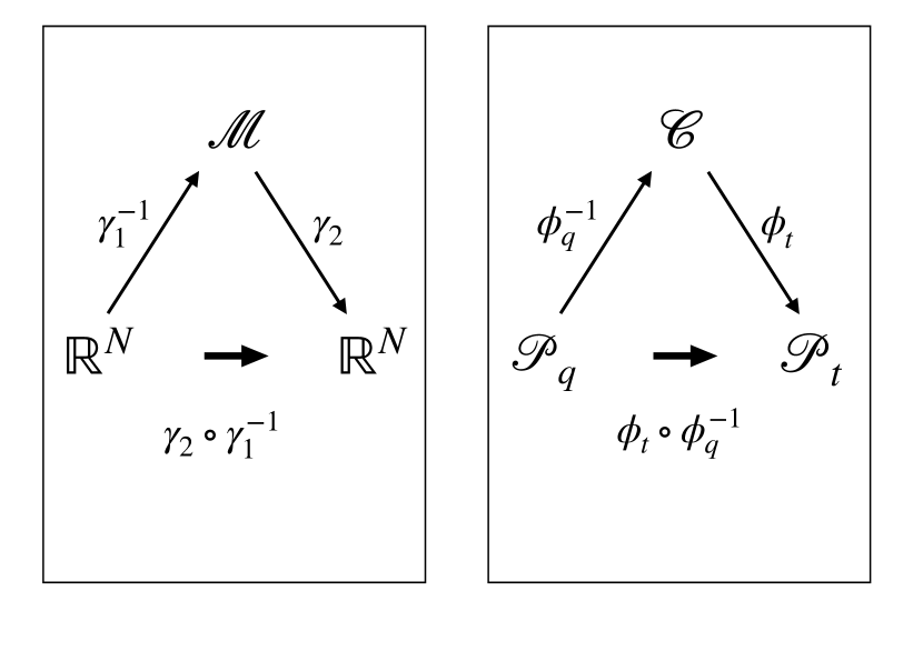
(a)

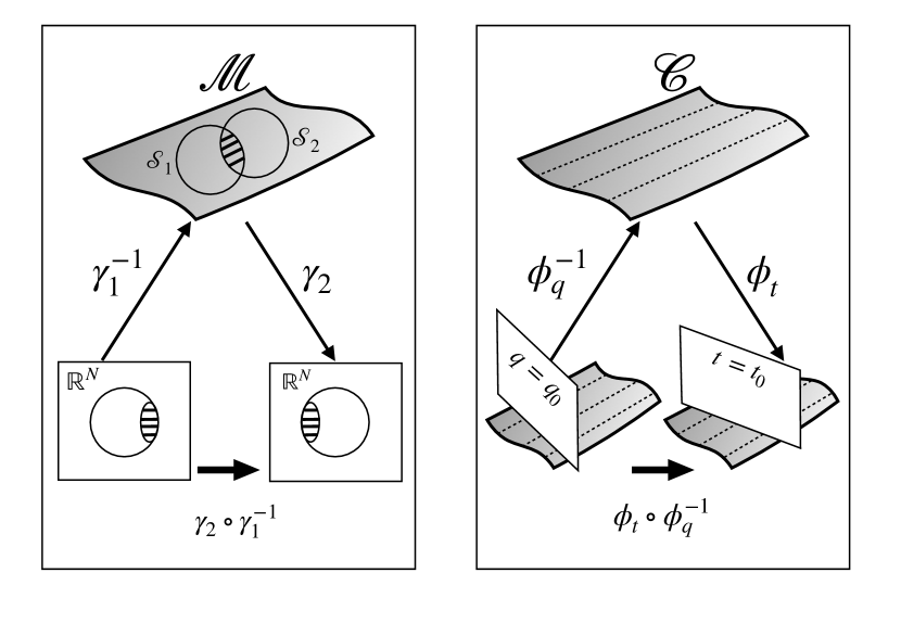
(b)

Figure 1: In (a), a schematic diagram illustrates the analogy between a change of coordinates and a change of gauge fixing is illustrated. On the left, we have a change of coordinates. On the right, we have a change of gauge fixing. In (b), we propose a pictorial, geometrical interpretation of the diagram. It is evident that a gauge fixing consists of defining a slice that cuts all the gauge histories, represented by dotted lines, once and only once.

The differences between DRFs and coordinates in GR are clear and can be summarised as follows. The total system of dynamical equations is deterministic when using a DRF and not deterministic when using coordinates. The variables used as coordinates are partial observables in the case of DRF, but not in the case of coordinates. Observables are gauge invariant if they are functions of the variables that constitute a DRF, but they are not gauge invariant when we use coordinates. For the sake of clarity, let us give a practical example of such differences. Let $\{X^{0},X^{i}\}$ be a set of coordinates and $\{T,Z^{i}\}$ a set of four scalar degrees of freedom similar to those introduced in the previous section for a dust. We consider the ADM space+time analysis of a model of GR plus a dust fluid. In total we have $6\crossproduct\infty^{3}$ degrees of freedom of the 3-metric $h_{ij}(X^{0},X^{i})$ written in coordinates and $4\crossproduct\infty^{3}$ physical degrees of freedom of the material system. By removing the $4\crossproduct\infty^{3}$ gauge degrees of freedom of the metric, $6\crossproduct\infty^{3}$ physical degrees of freedom remain. In the case where we use the material system as a reference frame, the metric $h_{ij}(T,Z^{i})$ written in terms of a DRF has $6\crossproduct\infty^{3}$ physical degrees of freedom. This is because we are able to use the dynamics of the material system to eliminate the gauge redundancy of the theory. Thus, repeating what was said in Section 3, the same dynamical theory, when written in relational terms (i.e. using a DRF) becomes deterministic and without any gauge freedom to be fixed. Furthermore, the quantity $h_{ij}(T,Z^{i})$ commutes with all constraints of the theory, hence it is a Dirac observable.

In the following, we want to propose a formal argument to distinguish a DRF from a coordinate system. This argument is based on the difference between transformations relating coordinate systems and DRFs, respectively. Let us analyse what we mean by ‘change a DRF’, assuming the case of ‘temporal reference frames’. In particular, we deal with the situation in which we have multiple internal degrees of freedom of the same physical system that can be used as a time variable. Thus, we have different physical degrees of freedom that could correspond to a gauge-fixed time variable. As in Section 3, we again use the parameterized Newtonian particle as an analogy. In this case, we could identify both the two variables $(q(\tau),t(\tau))$ on the extended configurational space as a relational internal clock. The map between the two different relational clocks $q$ and $t$ does not correspond to a passive diffeomorphism, but rather to a map relating the two different gauge-fixings selecting either $q$ or $t$ as a relational clock. In particular, this map will be an active diffeomorphism, namely a field-dependent map (see [Goeller et al.(2022)]), depending on the dynamical degrees of freedom $(q,t)$. In fact, the two gauge-fixing conditions for $q$ and $t$ can be seen as applications of an active diffeomorphism on the dynamical variables $q$ and $t$, respectively. Thus, the map between the two gauge-fixings is a composition of two active diffeomorphisms, which results in an active diffeomorphism. Geometrically, the map that links one time gauge choice to another is analogous to a coordinate transformation on a manifold. In this case, however, the role of the manifold is played by the space of gauge orbits defined on the constraint surface (see [Hoehn and Vanrietvelde(2020)] for further discussion on that point). The situation is summarised in Figure 1. In the figure, $\mathcal{M}$ and $\mathcal{C}$ indicate the spacetime manifold and the constraint surface, respectively. $\mathcal{P}_{q}$ and $\mathcal{P}_{t}$ represent the reduced phase space resulting from imposing the gauge condition $q=q_{0}$ and $t=t_{0}$, respectively. The $\gamma:\mathcal{S}\rightarrow\mathbb{R}^{N}$ map, already defined in Section 3, assigns a set of coordinates to the manifold points. We can assign two different sets of coordinates to the same point depending on whether we use the $\gamma_{1}$ or $\gamma_{2}$ map. A passive diffeomorphism consists in the composition map $\gamma_{2}\circ\gamma_{1}^{-1}$. The $\phi_{q}:\mathcal{C}\rightarrow\mathcal{P}_{q}$ map associates to each gauge orbit in $\mathcal{C}$ its intersection point with the gauge fixing surface setting $q$ as the relational clock. The same holds for $\phi_{t}:\mathcal{C}\rightarrow\mathcal{P}_{t}$, relative to time $t$. An active diffeomorphism consists in the composition map $\phi_{t}\circ\phi_{q}^{-1}$.

Naively, what is needed in order to change a gauge-fixing choice (say, e.g., we want to switch between relational evolution in $q$ and $t$ time) is to go back to the non-gauge-fixed level of the constraint surface (through the map $\phi_{q^{-1}}$), thus reintroducing a description in terms of the coordinate time $\tau$ and then fix a new gauge to choose the new temporal variable (through the map $\phi_{t}$). Of course, if we want to continue describing relational evolution in terms of the same gauge-selected internal clock, we are still free to go back to the non-gauge-fixed level, operate a passive diffeomorphism on the coordinate parameter $\tau$ and then choose the same gauge condition as before. We will see in the next section an example of this procedure within a cosmological setting.

6.1 Minisuperspace Bianchi I model

In the following, we will clarify in which sense a change of DRF can be implemented by a passive diffeomorphism. We will also provide a general-relativistic example of a change of DRF implemented by an active diffeomorphism. As mentioned in the introduction, and as we will make explicit below, we will actually be dealing with the case of gDRF. This is made clear by the fact that Bianchi’s models are vacuum models. For the sake of convenience, however, we will refer to generic DRFs in the remainder of the discussion, as the material-gravitational DRF distinction, while conceptually of great importance, is not decisive for the purpose of this section.

Let us consider a simple Minisuperspace model, corresponding to a Bianchi I model with two equal scale factors. This means that the configurational space is constituted only of one anisotropic variable $\beta(\tau)$ and the volume of the Universe variable $\alpha(\tau)$. Notice that the dynamical degrees of freedom, due to the model homogeneity, depend on coordinate time $\tau$ only. This system is formally similar to a parameterized system, that is evident once we make explicit the action

$$S=\int d\tau\left(p_{\alpha}\dot{\alpha}+p_{\beta}\dot{\beta}-N(\tau)\left[e^{-3\alpha/2}\left(-p_{\alpha}^{2}+p_{\beta}^{2}\right)\right]\right),$$ (5)

where $\dot{(...)}\equiv d(...)/d\tau$, the $p$’s are conjugate momenta to the corresponding variables. We observe that the extended Hamiltonian

$$H_{E}=Ne^{-3\alpha/2}(-p^{2}_{\alpha}+p^{2}_{\beta})$$ (6)

constitutes a first-class secondary constraint. By operating a deparametrization through a gauge choice on either variable $\alpha$ or $\beta$, we recover the so-called reduced phase space formulation of the theory. It is clear that we are completely free to choose either $\alpha$ or $\beta$ as possible internal clocks (thought as temporal DRFs) with respect to which the cosmological dynamics can be described. Evidently, in line with the discussion above, in this case we are dealing with two reference frames understood as degrees of freedom of the same physical system: the gravitational field under the assumptions of homogeneity, anisotropy and absence of matter. Let us assume we want to choose the variable $\alpha$ as the internal clock. Using the Hamilton’s equations

$$\begin{cases}\dot{\alpha}=-2p_{\alpha}Ne^{-3\alpha/2}\,,\,\dot{p}_{\alpha}=0\\ \dot{\beta}=2p_{\beta}Ne^{-3\alpha/2}\,,\,\dot{p}_{\beta}=0\end{cases}$$ (7)

we impose the following (partial) gauge condition

$$\dot{\alpha}=-2Np_{\alpha}e^{-3\alpha/2}\equiv 1,$$ (8)

which states just the coincidence (aside from a non-physical constant) of the variable $\alpha$ with the label time $\tau$. Imposing the gauge condition (8) turns out to be equivalent to fixing the following expression for the lapse function:

$$N(\alpha)\equiv-\frac{e^{3\alpha/2}}{{2p_{\alpha}}}\,.$$ (9)

Exactly as in the case of the parametrized particle given in Section 3, here we are able to solve Hamilton’s equations. Thus, we can invert the relation $\alpha(\tau)\leftrightarrow\tau(\alpha)$ and explicitly write the relational observable $\beta(\alpha)$. However, for the sake of our argument we choose to write relational observables via a complete gauge-fixing procedure. This amounts to choose a specific fixed value of $\alpha\equiv\alpha_{0}$, thus going to the reduced phase space. Here, this procedure consists of imposing the following gauge conditions:

$$\begin{cases}\dot{\alpha}\equiv 1\\ \alpha(\tau)\equiv\alpha_{0},\end{cases}$$ (10)

where the first condition represents the partial gauge-fixing implemented by the choice of the Lapse and the second one indicates a choice of a particular value of the quantity $\alpha(\tau)$ along the gauge orbit on the constraint surface. As a result, the relational observable $\beta(\alpha)$ is written as an evolving constant $\beta(\tau)|_{\alpha(\tau)=\alpha_{0}}:=\beta(\tau)-(p_{\beta}/p_{\alpha})[\alpha_{0}-\alpha(\tau)]$.

Recalling the link between the variable $\alpha$ and the volume of the Universe $V\propto e^{3\alpha/2}$, we see that the choice $\dot{\alpha}\equiv+1$ corresponds to an expanding Universe, while the choice $\dot{\alpha}\equiv-1$ corresponds to a collapsing one. We now demonstrate that we can switch from the gauge $\{\dot{\alpha}\equiv 1;\alpha=\alpha_{0}\}$ to the gauge $\{\dot{\alpha}\equiv-1;\alpha=\alpha_{0}\}$, that is from the expanding Universe to the contracting Universe case, through a passive diffeomorphism. Such a change of gauge can be interpreted as a change of DRF in the same sense as a frame re-coordination [Earman and Glymour(1978)].

Starting from the reduced phase space framework, we have to return to the non gauge-fixed level where the dynamics is encoded by both variables $\{\alpha(\tau),\beta(\tau)\}$. Subsequently, we perform the $\tau^{\prime}(\tau)=-\tau$ temporal passive diffeomorphism, and finally we fix again the same complete gauge choice (10), but now relative to coordinate time $\tau^{\prime}$.

In the notation used at the beginning of the section, such a change is implemented by the map $\phi_{\alpha}\circ\gamma_{\tau\rightarrow-\tau}\circ\phi_{\alpha}^{-1}\equiv\gamma_{\tau\rightarrow-\tau}$, which turns out to be a passive diffeomorphism, as we wanted to show. Here, the passive diffeomorphism composite map which changes the coordinate $\tau$ in $\tau^{\prime}=-\tau$ is represented by the symbol $\gamma_{\tau\rightarrow-\tau}$. The map $\phi_{\alpha}$ indicates the complete gauge choice (10). Of course, the map $\phi_{\beta}\circ\phi_{\alpha}^{-1}$ from the gauge choice $\{\dot{\alpha}\equiv 1;\alpha=\alpha_{0}\}$ to the gauge choice $\{\dot{\beta}\equiv 1;\beta=\beta_{0}\}$ is not a passive diffeomorphism, but an active diffeomorphism.

We point out that with such an example we also made it clear that $\alpha$ meets all the requirements of a (g)DRF, since its equations of motion are employed in the gauge-fixing procedure and the stress-energy tensor related to $\alpha$ is necessarily neglected, since it is not even definable. This, is due to the well-known fact that in GR there is not a meaningful local expression for the gravitational stress-energy tensor. Therefore, in such cosmological sector it is possible to use gravitational degrees of freedom to define a dynamical reference frame, as we have done with the variable $\alpha$ playing the role of the internal relational clock. In such a case, it is as if the gravitational field plays the role of both the dynamic variable and the reference frame relative to which the dynamics takes place.

7 Conclusion

We reviewed the notion of reference frame in physics and set out the need for the separation between the concepts of reference frame and coordinate system within GR.

We proposed three distinct classes of reference frames in GR, according to their increasing physical role in the gravitational dynamics. Indeed, we considered ‘idealised’ (IRF) those reference frames whose physical nature does not enter in any way into the physical picture, as ‘dynamical’ (DRF) those one which are associated with a specific set of dynamical equations, as ‘real’ (RRF) those whose stress-energy tensor also contributes to the EFEs.

We stressed how reference frames are often confused with coordinates in theoretical and experimental practice. This is because reference frames are approximated as IRFs and are supposed to coincide with coordinate systems. An IRF behaves as if it were a coordinate system. However, coordinates are representational tools of IRFs, which are constituted in fact by a set of partial observables to which a measuring device can be assigned. The difference between a coordinate system and a reference frame is also exemplified by the fact that a reference frame is employed within a relational approach and its degrees of freedom represent ‘physical coordinates’, whereas a coordinate system is a mathematical structure without a physical referent.

We proposed a comparison between the orthodox definition of a reference frame and the Brown-Kuchař dust. This discussion showed that the two definitions are similar. Nevertheless, the orthodox definition has some formal and conceptual difficulties in defining relational observables.

Finally, we presented a rather formal method to determine the difference between coordinate systems and DRFs. In short, a change of coordinate system is directly implemented by a passive diffeomorphism. A change of DRF can also be represented by a map which links different gauge-fixings. Only in the case where we do not change the choice of dynamical variables to be gauge-fixed, does a passive diffeomorphism directly represents a DRF change, which can be understood analogously to a frame re-coordination. This was clearly demonstrated using a simple Bianchi I Universe model.

The role of reference frames, as defined in this paper, has implications both for the increasingly studied notion of quantum reference frame and for future discussions on the nature of vacuum solutions of EFEs. In particular, it remains to be clarified how vacuum solutions can be reconsidered in terms of matter solutions where the stress-energy tensor is neglected. Consequently, the role of ‘idealised matter’ in the derivation of EFEs solutions in vacuum, such as the Schwarzschild solution describing a black hole, will have to be the subject of further analysis. Likewise, it remains to be clarified why and to what extent the approximation of reference frames as mere coordinates works so well that the difference between the two concepts can be overlooked. The measurement of gravitational waves, which is one of the greatest experimental successes in GR, is the clearest example of such a conundrum.

By introducing gDRFs, our work paves the way for future work on the analysis of gravitational, non-material reference frames. The close connection to the problem of defining a stress-energy tensor for the gravitational field underlines the relevance of these issues to the foundations of GR. In summary, in this paper we stated the necessity to distinguish between the terms reference frame and coordinate system in GR. This distinction, while conceptually relevant, is sometimes blurred because in some cases, as in the case of IRFs, it has no bearing on theoretical practice. In other circumstances it becomes unavoidable in light of the relevant result of being able to write local Dirac observable in GR. However, clarifying this distinction and refining the definitions provided in the literature so far may have significant implications in the foundations of Einsteinian theory of gravity.

References

- [Abbott et al.(2016)] B. P. Abbott et al. Observation of gravitational waves from a binary black hole merger. Phys. Rev. Lett., 116:061102, Feb 2016. doi: 10.1103/PhysRevLett.116.061102. URL https://link.aps.org/doi/10.1103/PhysRevLett.116.061102.
- [Arnowitt et al.(1960)] R. Arnowitt et al. Canonical variables for general relativity. Physical Review, 117(6):1595–1602, Mar. 1960. doi: 10.1103/physrev.117.1595. URL https://doi.org/10.1103/physrev.117.1595.
- [Belot and Earman(2001)] G. Belot and J. Earman. Pre-Socratic quantum gravity, page 213–255. Cambridge University Press, 2001. doi: 10.1017/CBO9780511612909.011.
- [Bergmann(1961a)] P. G. Bergmann. Observables in general relativity. Reviews of Modern Physics, 33(4):510–514, Oct. 1961a. doi: 10.1103/revmodphys.33.510. URL https://doi.org/10.1103/revmodphys.33.510.
- [Bergmann(1961b)] P. G. Bergmann. ”gauge-invariant” variables in general relativity. Phys. Rev., 124:274–278, Oct 1961b. doi: 10.1103/PhysRev.124.274. URL https://link.aps.org/doi/10.1103/PhysRev.124.274.
- [Bergmann(1962)] P. G. Bergmann. The general theory of relativity. 1962.
- [Bergmann and Komar(1960)] P. G. Bergmann and A. B. Komar. Poisson brackets between locally defined observables in general relativity. Phys. Rev. Lett., 4:432–433, Apr 1960. doi: 10.1103/PhysRevLett.4.432. URL https://link.aps.org/doi/10.1103/PhysRevLett.4.432.
- [Bianchi(1989)] L. Bianchi. Sugli spazi a tre dimensioni che ammettono un gruppo continuo di movimenti. Memorie di Matematica e di Fisica della Societa Italiana delle Scienze, Serie Terza 11, pp. 267–352, 1989.
- [Bradley(2021)] C. Bradley. The non-equivalence of einstein and lorentz. The British Journal for the Philosophy of Science, 72(4):1039–1059, Dec. 2021. doi: 10.1093/bjps/axz014. URL https://doi.org/10.1093/bjps/axz014.
- [Brown(2005)] H. R. Brown. Physical Relativity. Clarendon Press, Oxford, England, Dec. 2005.
- [Brown and Kuchař(1995)] J. D. Brown and K. V. Kuchař. Dust as a standard of space and time in canonical quantum gravity. Physical Review D, 51(10):5600–5629, May 1995. doi: 10.1103/physrevd.51.5600. URL https://doi.org/10.1103/physrevd.51.5600.
- [Dirac(2001)] P. Dirac. Lectures on Quantum Mechanics. Belfer Graduate School of Science, monograph series. Dover Publications, 2001. ISBN 9780486417134. URL https://books.google.it/books?id=GVwzb1rZW9kC.
- [DiSalle(2020)] R. DiSalle. Space and Time: Inertial Frames. In E. N. Zalta, editor, The Stanford Encyclopedia of Philosophy. Metaphysics Research Lab, Stanford University, Winter 2020 edition, 2020.
- [Domagała et al.(2010)] M. Domagała et al. Gravity quantized: Loop quantum gravity with a scalar field. Phys. Rev. D, 82:104038, Nov 2010. doi: 10.1103/PhysRevD.82.104038. URL https://link.aps.org/doi/10.1103/PhysRevD.82.104038.
- [Earman(1974)] J. Earman. Covariance, invariance, and the equivalence of frames. Foundations of Physics, 4(2):267–289, June 1974. doi: 10.1007/bf00712691. URL https://doi.org/10.1007/bf00712691.
- [Earman(2006)] J. Earman. The implications of general covariance for the ontology and ideology of spacetime. In D. Dieks, editor, The Ontology of Spacetime, pages 3–24. Elsevier, 2006.
- [Earman and Glymour(1978)] J. Earman and C. Glymour. Lost in the tensors: Einstein's struggles with covariance principles 1912–1916. Studies in History and Philosophy of Science Part A, 9(4):251–278, Dec. 1978. doi: 10.1016/0039-3681(78)90008-0. URL https://doi.org/10.1016/0039-3681(78)90008-0.
- [Earman and Norton(1987)] J. Earman and J. Norton. What price spacetime substantivalism? the hole story. British Journal for the Philosophy of Science, 38(4):515–525, 1987. doi: 10.1093/bjps/38.4.515.
- [Einstein(1905)] A. Einstein. Zur elektrodynamik bewegter körper. Annalen der Physik, 322(10):891–921, 1905. doi: 10.1002/andp.19053221004. URL https://doi.org/10.1002/andp.19053221004.
- [Einstein(1916)] A. Einstein. Die grundlage der allgemeinen relativitätstheorie. Annalen der Physik, 354(7):769–822, 1916. doi: 10.1002/andp.19163540702. URL https://doi.org/10.1002/andp.19163540702.
- [Giacomini et al.(2019)] F. Giacomini et al. Quantum mechanics and the covariance of physical laws in quantum reference frames. Nature Communications, 10(1), Jan. 2019. doi: 10.1038/s41467-018-08155-0. URL https://doi.org/10.1038/s41467-018-08155-0.
- [Giesel et al.(2010)] K. Giesel et al. Manifestly gauge-invariant general relativistic perturbation theory: I. foundations. Classical and Quantum Gravity, 27(5):055005, Feb. 2010. doi: 10.1088/0264-9381/27/5/055005. URL https://doi.org/10.1088/0264-9381/27/5/055005.
- [Goeller et al.(2022)] C. Goeller et al. Diffeomorphism-invariant observables and dynamical frames in gravity: reconciling bulk locality with general covariance. 2022. doi: 10.48550/ARXIV.2206.01193. URL https://arxiv.org/abs/2206.01193.
- [Gryb and Thébault(2016)] S. Gryb and K. P. Y. Thébault. Regarding the ‘hole argument’ and the ‘problem of time’. Philosophy of Science, 83(4):563–584, Oct. 2016. doi: 10.1086/687262. URL https://doi.org/10.1086/687262.
- [Henneaux and Teitelboim(1994)] M. Henneaux and C. Teitelboim. Quantization of gauge systems. Princeton University Press, Princeton, NJ, Aug. 1994.
- [Hoehn and Vanrietvelde(2020)] P. Hoehn and A. Vanrietvelde. How to switch between relational quantum clocks. New Journal of Physics, 22, 12 2020. doi: 10.1088/1367-2630/abd1ac.
- [Komar(1958)] A. Komar. Construction of a complete set of independent observables in the general theory of relativity. Phys. Rev., 111:1182–1187, Aug 1958. doi: 10.1103/PhysRev.111.1182. URL https://link.aps.org/doi/10.1103/PhysRev.111.1182.
- [Misner(1969)] C. W. Misner. Quantum cosmology. i. Phys. Rev., 186:1319–1327, Oct 1969. doi: 10.1103/PhysRev.186.1319. URL https://link.aps.org/doi/10.1103/PhysRev.186.1319.
- [Norton(1985)] J. Norton. What was einstein's principle of equivalence? Studies in History and Philosophy of Science Part A, 16(3):203–246, Sept. 1985. doi: 10.1016/0039-3681(85)90002-0. URL https://doi.org/10.1016/0039-3681(85)90002-0.
- [Norton(1989)] J. Norton. Coordinates and covariance: Einstein's view of space-time and the modern view. Foundations of Physics, 19(10):1215–1263, Oct. 1989. doi: 10.1007/bf00731880. URL https://doi.org/10.1007/bf00731880.
- [Norton(1993)] J. D. Norton. General covariance and the foundations of general relativity: Eight decades of dispute. Reports of Progress in Physics, 56:791–861, 1993.
- [Norton(2012)] J. D. Norton. Approximation and idealization: Why the difference matters. Philosophy of Science, 79(2):207–232, Apr. 2012. doi: 10.1086/664746. URL https://doi.org/10.1086/664746.
- [Penrose and Rindler(1987)] R. Penrose and W. Rindler. Cambridge monographs on mathematical physics spinors and space-time: Two-spinor calculus and relativistic fields volume 1. Cambridge University Press, Cambridge, England, Feb. 1987.
- [Pitts(2022)] J. B. Pitts. Peter bergmann on observables in hamiltonian general relativity: A historical-critical investigation. Studies in History and Philosophy of Science, 95:1–27, Oct. 2022. doi: 10.1016/j.shpsa.2022.06.012. URL https://doi.org/10.1016/j.shpsa.2022.06.012.
- [Pooley(2017)] O. Pooley. Background independence, diffeomorphism invariance and the meaning of coordinates. In Towards a Theory of Spacetime Theories, pages 105–143. Springer New York, 2017. doi: 10.1007/978-1-4939-3210-8˙4. URL https://doi.org/10.1007/978-1-4939-3210-8_4.
- [Pooley and Read(2021)] O. Pooley and J. A. M. Read. On the mathematics and metaphysics of the hole argument. The British Journal for the Philosophy of Science, 0(ja):null, 2021. doi: 10.1086/718274. URL https://doi.org/10.1086/718274.
- [Read(2020)] J. Read. Functional gravitational energy. The British Journal for the Philosophy of Science, 71(1):205–232, Mar. 2020. doi: 10.1093/bjps/axx048. URL https://doi.org/10.1093/bjps/axx048.
- [Rovelli(1991a)] C. Rovelli. What is observable in classical and quantum gravity? Classical and Quantum Gravity, 8(2):297–316, Feb. 1991a. doi: 10.1088/0264-9381/8/2/011. URL https://doi.org/10.1088/0264-9381/8/2/011.
- [Rovelli(1991b)] C. Rovelli. Quantum reference systems. Classical and Quantum Gravity, 8(2):317–331, Feb. 1991b. doi: 10.1088/0264-9381/8/2/012. URL https://doi.org/10.1088/0264-9381/8/2/012.
- [Rovelli(2002a)] C. Rovelli. Gps observables in general relativity. Phys. Rev. D, 65:044017, Jan 2002a. doi: 10.1103/PhysRevD.65.044017. URL https://link.aps.org/doi/10.1103/PhysRevD.65.044017.
- [Rovelli(2002b)] C. Rovelli. Partial observables. Physical Review D, 65(12), jun 2002b. doi: 10.1103/physrevd.65.124013.
- [Rovelli(2004)] C. Rovelli. Quantum Gravity. Cambridge University Press, 2004. URL https://doi.org/10.1017/CBO9780511755804.
- [Rovelli(2014)] C. Rovelli. Why gauge? Foundations of Physics, 44(1):91–104, Jan. 2014. doi: 10.1007/s10701-013-9768-7. URL https://doi.org/10.1007/s10701-013-9768-7.
- [Rovelli and Gaul(2000)] C. Rovelli and M. Gaul. Loop quantum gravity and the meaning of diffeomorphism invariance. In Lecture Notes in Physics, pages 277–324. Springer Berlin Heidelberg, 2000. doi: 10.1007/3-540-46634-7˙11. URL https://doi.org/10.1007/3-540-46634-7_11.
- [Rovelli and Smolin(1994)] C. Rovelli and L. Smolin. The physical hamiltonian in nonperturbative quantum gravity. Physical Review Letters, 72(4):446–449, Jan. 1994. doi: 10.1103/physrevlett.72.446. URL https://doi.org/10.1103/physrevlett.72.446.
- [Tambornino(2012)] J. Tambornino. Relational observables in gravity: a review. Symmetry, Integrability and Geometry: Methods and Applications, Mar. 2012. doi: 10.3842/sigma.2012.017. URL https://doi.org/10.3842/sigma.2012.017.
- [Thébault(2012)] K. P. Y. Thébault. Symplectic reduction and the problem of time in nonrelativistic mechanics. The British Journal for the Philosophy of Science, 63(4):789–824, Dec. 2012. doi: 10.1093/bjps/axr045. URL https://doi.org/10.1093/bjps/axr045.
- [Thiemann(2006)] T. Thiemann. Solving the problem of time in general relativity and cosmology with phantoms and k – essence. 2006. doi: 10.48550/ARXIV.ASTRO-PH/0607380. URL https://arxiv.org/abs/astro-ph/0607380.
- [Wald(1984)] R. M. Wald. General Relativity. University of Chicago Press, Chicago, IL, June 1984.
- [Weatherall(2018)] J. O. Weatherall. Regarding the hole argument. British Journal for the Philosophy of Science, 69(2):329–350, 2018. doi: 10.1093/bjps/axw012.