Estimation of the Number Needed to Treat, the Number Needed to be Exposed, and the Exposure Impact Number with Instrumental Variables

Abstract

The number needed to treat (NNT) is an efficacy index defined as the average number of patients needed to treat to attain one additional treatment benefit. In observational studies, specifically in epidemiology, the adequacy of the populationwise NNT is questionable since the exposed group characteristics may substantially differ from the unexposed. To address this issue, groupwise efficacy indices were defined: the Exposure Impact Number (EIN) for the exposed group and the Number Needed to be Exposed (NNE) for the unexposed. Each defined index answers a unique research question since it targets a unique sub-population. In observational studies, the group allocation is typically affected by confounders that might be unmeasured. The available estimation methods that rely either on randomization or the sufficiency of the measured covariates for confounding control will result in inconsistent estimators of the true NNT (EIN, NNE) in such settings. Using Rubin’s potential outcomes framework, we explicitly define the NNT and its derived indices as causal contrasts. Next, we introduce a novel method that uses instrumental variables to estimate the three aforementioned indices in observational studies. We present two analytical examples and a corresponding simulation study. The simulation study illustrates that the novel estimators are consistent, unlike the previously available methods, and their confidence intervals meet the nominal coverage rates. Finally, a real-world data example of the effect of vitamin D deficiency on the mortality rate is presented.

1 Introduction

The number needed to treat (NNT) is an efficacy index commonly used in the analysis of randomized controlled trials (RCT), as well as in epidemiology and meta-analysis.[1, 2, 3, 4, 5, 6] It is assumed that there are two groups - treated and untreated. In observational studies, specifically in epidemiology, the adequacy of the populationwise NNT is questionable since the treated group characteristics may substantially differ from the untreated group. Therefore, groupwise efficacy indices were defined.[7] Particularly, for the treated group, the defined groupwise measure is the exposure impact number (EIN), and for the untreated group is the number needed to be exposed (NNE). Each one of these indices answers a unique research question. The populationwise NNT might be of interest if the treatment (exposure) is considered mandatory for the whole population, while EIN and NNE might be of interest in scenarios where the exposure is elective. The term treatment is replaced with the term exposure to be consistent with the common terminology in observational studies.

The NNT was originally defined as the average number of patients to be treated to observe one less adverse effect.[8, 9] Another common definition is the average number of patients to be treated to observe one more beneficial outcome due to treatment (treatment benefit). These are two equivalent definitions since avoiding one more adverse effect can be defined as the treatment benefit. As we are focusing on epidemiological studies, the term treatment benefit is replaced with the term exposure benefit. Our target parameters in this article are the three indices; EIN, NNE, and NNT. The aforementioned definitions of the NNT can be readily applied to define the EIN and the NNE by restricting the target population to the exposed and unexposed groups, respectively.

Several authors [10, 11, 12, 13, 14] have noticed that the causal meaning of the NNT and its derived indices (EIN, NNE) is embedded in their very definition. Hence, we will use Rubin’s potential outcomes framework[15] to define all three indices. Since any of these indices is a one-to-one mapping of the exposure benefit in the corresponding (sub)population, we start with its formal definition. Let $Y_{1}$ be the potential outcome for a given individual if exposed, and $Y_{0}$ be the potential outcome for the same individual if the individual was not exposed. Let $A$ be the exposure indicator where its realization is denoted by the subscript $a$, such that $a=1$ denotes exposure and $a=0$ non-exposure. Let $I_{a}$ be the potential dichotomous outcome if the exposure $A$ is set to $a$, $a\in\{0,1\}$. If the potential outcome is binary, then $I_{a}\equiv Y_{a}$, $a\in\{0,1\}$. Otherwise, a dichotomization is performed, e.g., $I_{a}\equiv I\{Y_{a}\leq\tau\}$, for $a\in\{0,1\}$. The formal definition of the exposure benefit is $\{I_{1}=1,I_{0}=0\}$. Namely, a benefit that is caused by the exposure such that without the exposure, no benefit will occur. Therefore, the formal definition of the exposure benefit probability[13] is

$$p_{b}=P(I_{1}=1,I_{0}=0).$$ (1)

Another common definition of the exposure benefit is $E[I_{1}-I_{0}]=P(I_{1}=1)-P(I_{0}=1).$ This quantity is also known as the average treatment effect (ATE). However, it is qualitatively different from $p_{b}$ as defined in eq. (1). Particularly, one can expand $p_{1}=P(I_{1}=1)=P(I_{1}=1,I_{0}=0)+P(I_{1}=1,I_{0}=1)$, and $p_{0}=P(I_{0}=1)=P(I_{1}=1,I_{0}=1)+P(I_{1}=0,I_{0}=1)$. Therefore, the ATE can be expressed as

$$p_{1}-p_{0}=p_{b}-P(I_{1}=0,I_{0}=1).$$

Namely, whenever the treatment can be harmful, i.e., $P(I_{1}=0,I_{0}=1)>0$, ATE $\neq p_{b}$. In such a case, the support set of ATE is $[-1,1]$. Therefore, it is not a probability. Several authors [13, 16, 17] defined the NNT (EIN, NNE) explicitly as the reciprocal number of the exposure benefit probability $p_{b}$. Other authors [18, 19] refrained from explicitly defining the NNT as the inverse of a probability; however, they assumed that $p_{1}\geq p_{0}$. This assumption restricts the ATE to $[0,1]$, and thus it can be interpreted as a probability, even if it was not explicitly done so. However, it is still not the same probability as in eq. (1) since it allows for the exposure to be harmful for a certain sub-population, as long as it is beneficial on average. In order to unify the different approaches, we suggest using the monotonicity assumption.[16, 20, 21] Formally, assuming $I_{1}\geq I_{0}$, for any individual in the target population. In other words, we assume that the treatment is not harmful. In such a case, the ATE is non-negative and equals the exposure benefit probability $p_{b}$. Hence the NNT (EIN, NNE) is consistently defined as its inverse. Without the monotonicity assumption, the target parameter remains the ATE. However, in such a case, the interpretation of the estimates is different. Namely, the EIN, NNE, and NNT are estimated by the reciprocal of the ATE in the corresponding group, which differs from the reciprocal of the exposure benefit probability as defined in eq. (1). In other words, relaxing the monotonicity assumption changes the interpretation of the target parameter but does not affect the presented methodology.

In order to intuitively understand the NNT, let $N$ be the number of exposed individuals. Thus, $NE[I_{1}]=Np_{1}$ is the number of beneficial outcomes if all $N$ individuals are exposed. Analogically, $NE[I_{0}]=Np_{0}$ is the number of beneficial outcomes if all $N$ individuals are not exposed. Therefore, the NNT is defined as the quantity $N$ that solves the following equation

$$N(p_{1}-p_{0})=1.$$

Using the monotonicity assumption, the solution is the reciprocal of the exposure benefit probability $p_{b}$, i.e., $1/p_{b}$. Alternatively, assume a random variable $N_{b}$ that counts the number of exposed individuals out of an infinitely large super-population until the first exposure benefit occurs. Then $N_{b}$ follows geometric distribution in which the expected value is known to be

$$E[N_{b}]=\frac{1}{p_{b}}=\frac{1}{p_{1}-p_{0}}.$$

Namely, $E[N_{b}]$ is the expected number of people to be exposed to observe the first exposure benefit. Using these two motivational examples, we arrive at the same original Laupcais’ et al.[8] definition of the NNT. Assuming strict monotonicity, i.e., $I_{1}>I_{0}$, at least for one individual, implies $p_{b}>0$. Due to sampling variability, this definition may result in negative point estimators of the NNT. Such estimators lead to difficulties in their interpretation,[22, 23, 24, 25, 9] bi-modal sample distribution,[22] and infinite disjoint confidence intervals (CIs). All these non-desirable properties occur due to singularity at $0$ of the original definition. Vancak et al.[26] resolved the pitfall of singularity at $0$ by modifying the original definition of the NNT. The modified NNT is

$$\text{NNT}\equiv g(p_{b})=\begin{cases}1/p_{b},\quad p_{b}>0\\ \infty,\quad\,\,\,\,\,p_{b}\leq 0\,.\end{cases}$$ (2)

We adopt this modification for all three indices; EIN, NNE, and NNT. Namely, these indices are defined by applying the function $g$  as in eq.(2) to the corresponding exposure benefit probability.

The fundamental problem of causal inference is that it is impossible to observe both $I_{1}$ and $I_{0}$ within the same individual,[27] as the individual is either exposed or unexposed. Formally, $I=I_{0}I\{A=0\}+I_{1}I\{A=1\}$. The counterfactuals-based definition highlights the main challenge with the three indices - their estimation. The parameter $p_{b}$ cannot be estimated directly since we cannot distinguish between a successful outcome due to exposure (i.e., exposure benefit) and a successful outcome not due to exposure (i.e., non-exposure benefit) on an individual level. Therefore, a straightforward practice to estimate $p_{b}$ is using randomized controlled trials (RCTs) where the exposure group is used to estimate $p_{1}$, and the control (unexposed) group to estimate $p_{0}$.

In order to define the EIN and NNE, we need first define the general exposure benefit probability as a function of the exposure indicator $A$

$$p_{b}(A)=P(I_{1}=1,I_{0}=0|A)=E[I_{1}-I_{0}|A],$$ (3)

where the marginal exposure benefit probability $p_{b}$ is obtained by $E[p_{b}(A)]$. To define the groupwise exposure benefit probability $p_{b}(a)$, we set the exposure $A$ in eq. (3) to a fixed value $a$. Namely, $p_{b}(a)=E[I_{1}-I_{0}|A=a],$ $a\in\{0,1\}$, where $p_{b}(0)$ and $p_{b}(1)$ are the exposure benefit probabilities for the unexposed and the exposed groups, respectively. Consequently, the EIN is defined as $g(p_{b}(1))$ and the NNE as $g(p_{b}(0))$. If the exposure is randomized, then $p_{b}(0)=p_{b}(1)=p_{b}$, and EIN = NNE = NNT. Otherwise, generally, $p_{b}(0)\neq p_{b}(1)$, and the marginal exposure benefit probability is their weighted mean, i.e., $p_{b}=E[p_{b}(A)]$. Next, we define the general conditional exposure benefit probability. Let $L$ be background characteristics, such as age, sex, and other relevant features measured in the study baseline. Therefore, the general conditional exposure benefit probability is

$$p_{b}(A,L)=P(I_{1}=1,I_{0}=0|A,L)=E[I_{1}-I_{0}|A,L].$$ (4)

The conditional exposure benefit probability for the $a$th group $p_{b}(a;L)$ is obtained by setting the exposure indicator $A$ to a fixed value $a$ in eq. (4), i.e., $p_{b}(a;L)=p_{b}(A=a,L)$. The groupwise marginal exposure benefit probabilities $p_{b}(0)$, $p_{b}(1)$, can be obtained by averaging the groupwise conditional exposure benefit probability over $L$ in the corresponding group. Consequently, the true EIN and NNE are obtained by $g(E[p_{b}(1;L)|A=1])$ and $g(E[p_{b}(0;L)|A=0])$, respectively. Analogically, the true NNT is obtained by $g(E[p_{b}(A,L)])$.

The available estimation methods rely either on randomization of exposure allocation or on sufficiency of $L$ for confounding control.[14, 12, 7] Formally, in non-randomized settings, the counterfactual part $E[I_{a}|A=1-a]$ of the groupwise exposure benefit probability $p_{b}(a)$ is identified as

$$E[I_{a}|A=1-a]=E[E[I|A=a,L]|A=1-a],$$

only if $L$ is assumed to be sufficient for confounding control. This assumption is hardly realistic in most observational studies. In this article, we focus on estimating the marginal EIN, NNE, and NNT in observational studies where there are no measured confounders or the measured confounders $L$ are insufficient for confounding control. The proposed estimation method relies on instrumental variables (IVs), which, under appropriate assumptions, allows for consistent estimation of the three indices. An IV $Z$ is a variable that is associated with the exposure $A$, affects the outcome $I$ only through the exposure, and is not confounded with the outcome by unmeasured confounders $U$. Please refer to Figure 1 for a graphical illustration of an IV. The use of IV regression methods is a common practice in epidemiological studies. However, to the authors’ knowledge, IV regression has not yet been used to estimate the EIN, NNE, or NNT. A possible application of the two-stage least-squares (TSLS)[21] method is restrictive, since it requires a linear model with a normally distributed outcome. Namely, the TSLS regression requires specific assumptions on the original latent data-generating process prior to dichotomization. However, since the outcome is assumed to be dichotomous for the NNT (NNE, EIN) calculations, the TSLS is not always feasible in such settings since the estimation must be performed on the original data scale, which is not always available. On the other hand, our method is based on modeling the already dichotomous outcome’s causal structure, whether the outcome was dichotomized or is naturally dichotomous. Such an approach aligns with the usual workflow where the data analysis starts after possible dichotomization. Notably, this practice has disadvantages - dichotomization results in a loss of Fisher information and, therefore, a decrease in statistical power.[28, 29] However, dichotomization is unavoidable if the researcher uses the NNT (NNE, EIN) indices on non-dichotomous data. Whether the dichotomization is justified is usually a clinical question, which is out of the scope of our study. Unlike the TSLS method, our approach allows the structural model to consider arbitrary link functions and does not require assumptions on possible latent processes. This makes the novel method more appealing and applicable to various applications.

The rest of the paper is structured as follows: Section 2 defines and models the exposure benefit probabilities in observational studies using generalized structural mean models. Section 3 provides two illustrative examples of the model presented earlier. In particular, we introduce the double logit and the double probit models. Section 4 introduces the novel estimation method. In Section 5, we conduct a simulation study to compare the new estimation method to the previously available methods. Section 6 presents an analysis of real-world data. In this analysis, we use the aforementioned indices to measure the effect of vitamin D deficiency on mortality. Section 7 concludes the study by summarizing its main results and discussing future research directions.

Figure 1: A causal structure of a valid IV. $I$ is the outcome variable, $A$ is exposure, and $Z$ is the instrument. $U$ represents all unmeasured confounders of $A$ and $I$, whereas $L$ represents all measured confounders. The instrument $Z$ affects $I$ only through the exposure $A$, and is not confounded with the outcome by the unmeasured variables.

2 Modeling the exposure benefit probability

2.1 Instrumental variables

Let $\{L,U\}$ be a set of all confounders of the exposure $A$ and the outcome $I$, such that $L$ denotes measured confounders and $U$ denotes unmeasured confounders. In scenarios where $U=\emptyset$, $L$ is sufficient for confounding control. However, in many observational studies $U\neq\emptyset$, thus the measured confounders $L$ are insufficient for confounding control. In such a case, the estimation of the conditional and marginal exposure benefit probabilities by adjusting for the measured confounders $L$ will result in inconsistent estimators of the exposure benefit probabilities and their corresponding efficacy indices. A possible approach to address the issue of confounding bias to use instrumental variables (IVs). Formally, an IV $Z$ is a variable that is (1) relevant, i.e., is associated with exposure $A$, (2) exogenous, i.e., is not associated with unmeasured confounders, and (3) affects the outcome $Y$ only through the exposure $A$ (exclusion). The exclusion and the exogeneity assumptions can be compactly formulated using counterfactuals: $I_{a}\rotatebox[origin={c}]{90.0}{$\models$}Z|L$, $a\in\{1,0\}$.[30] For graphical illustration of a valid IV please refer to Figure 1. In the following subsection, we introduce generalized structural mean models that are used to model the exposure benefit probabilities and the corresponding indices. Since we assume that $L$ is insufficient for confounding control, the observed and the potential outcomes are conditionally associated with the instrument $Z$, given exposure $A$. This occurs since conditioning on the exposure opens a non-causal path from an outcome $I$ to $Z$ through the unmeasured confounder $U$, on which $A$ is a collider. Therefore, both the causal and the associative models below are conditioned on $Z$.

2.2 Generalized structural mean model

We use a two-stage modeling approach. In the first stage, we specify a semiparametric generalized structural mean model (GSMM), and in the second stage we specify a traditional association model. The GSMM of the first stage specifies the mean causal effect for the exposed (unexposed) individuals, while the second stage association model is required for the identification of the former. Formally, for a general link function $\xi$, we assume that the GSMM is

$$\xi\left(E[I_{1}|Z,L,A=a]\right)-\xi\left(E[I_{0}|Z,L,A=a]\right)=m_{a}^{T}(L)\psi_{a},\quad a\in\{0,1\},$$ (5)

where $\psi_{a}\in\Psi_{a}$ is the vector of causal parameters for the $a$th group, $a\in\{0,1\}$, and $\text{dim}(m_{a}(L))=\text{dim}(\psi_{a})$. The composition of the vector-valued function $m_{a}(L)$ defines the exact form of the causal model and may allow for interactions between $L$ and the exposure $A$ in the $a$th group. In addition, since the causal parameters also depend on the group $a$, it allows for a distinct model for each exposure group $a\in\{0,1\}$. According to the consistency assumption, $E[I_{a}|Z,L,A=a]=E[I|Z,L,A=a]$.[30] Therefore, this part of the model is identifiable from the observed data. However, the identification of the counterfactual part $E[I_{a}|L,Z,A=1-a]$ requires a model and a valid IV. Particularly, the conditional independence of $I_{a}$ and $Z$ given $L$ implies the mean independence as presented in the following equality

$$E[I_{a}|Z,L]=E[I_{a}|L],\quad a\in\{0,1\}.$$ (6)

To estimate the conditional benefit probabilities, we need to specify the second stage model - a statistical association model for the observed outcomes. Let $\eta$ be a link function, then the association model is defined as $\eta\left(E[I|Z,L,A]\right)$. A notable distinction between the association and the causal model is that the association model might be dependent on the instrument $Z$. If $L$ is insufficient for confounding control; then the observed outcome $I$ will be associated with the instrument $Z$. Generally, the two link functions might be different. For example, if $\eta$ is the probit link function, and $\xi$ is the logit link function, we have a probit-logit joint model. However, in many scenarios, one may assume that $\xi=\eta$. For example, suppose there are no unmeasured confounders, and the two link functions are the same. In that case, the parameters of the association model are equal to the corresponding parameters of the structural model. GSMMs with the same link function $\xi$ for the structural and the association model are referred to as double $\xi$ models, where $\xi$ is replaced with the relevant link function. The form of the general conditional exposure benefit probability (4) is

$$p_{b}(Z,L,A)=E[I_{1}-I_{0}|Z,L,A].$$ (7)

Since this probability depends on the exposure $A$, to obtain the conditional populationwise exposure benefit probability, we average it over the conditional distribution of $A$ given $Z$ and $L$,

$$p_{b}(Z,L)=E[p_{b}(Z,L,A)|Z,L].$$ (8)

Consequently, the marginal populationwise exposure benefit probability $p_{b}$ is obtained by averaging $p_{b}(Z,L)$ over the joint distribution of $Z$ and $L$, i.e.,

$$p_{b}=E[p_{b}(Z,L)]=E[I_{1}-I_{0}].$$ (9)

Thus, the populationwise NNT can be obtained by applying $g$ tp $p_{b}$, i.e., $g(p_{b})$. The conditional exposure benefit probability for the $a$th group is obtained by setting the exposure indicator $A$ to a fixed value $a$ in eq. (7), i.e.,

$$p_{b}(a;Z,L)=E[I_{1}-I_{0}|Z,L,A=a],\quad a\in\{0,1\}.$$ (10)

By calculating the expectation w.r.t. the joint conditional distribution of $Z$, $L$, in the $a$th group, one can recover the marginal probability of the exposure benefit in the $a$th group, and consequently the EIN and the NNE. Namely, the groupwise exposure benefit probability is given by

$$p_{b}(a)=E[p_{b}(a;Z,L)],\quad a\in\{0,1\},$$ (11)

where the EIN and NNE are obtained by applying $g$ to $p_{b}(1)$ and $p_{b}(0)$, respectively. Assuming that $\xi=\eta$, the general conditional exposure benefit probability can be formulated as

$$p_{b}(Z,L,A,\psi) =\xi^{-1}\left(\xi(E[I|Z,L,A])+m^{T}_{0}(L)\psi_{0}(1-A))\right)$$ (12)

$$-\xi^{-1}\left(\xi(E[I|Z,L,A])-m^{T}_{1}(L)\psi_{1}A\right).$$

The conditional exposure benefit probability for the $a$th group, $p_{b}(a;Z,L,\psi_{a})$, is obtained by setting the exposure $A$ to a fixed value $a$ in eq. (12), namely, $p_{b}(a;Z,L,\psi_{a})=p_{b}(Z,L,a,\psi)$, $a\in\{0,1\}$. The exact form of the conditional populationwise and groupwise exposure benefit probabilities depend on the GSMM and the specified association model.

3 Example

3.1 The double logit model

Assume a binary outcome $I\in\{0,1\}$, a binary exposure $A\in\{0,1\}$, and a binary instrument $Z\in\{0,1\}$. Assume there are no measured confounders, i.e., $L=\emptyset$ and $m(L)=1$. For the logit link function $\xi$, we define the GSMM (5) as

$$\text{logit}\left(E[I_{1}=1|Z,A=a]\right)-\text{logit}\left(E[I_{0}=1|Z,A=a]\right)=\psi_{a},\quad a\in\{0,1\},$$ (13)

where $\text{logit}(x)=\ln\left(\frac{x}{1-x}\right)$. Notably, there are two causal parameters $\psi=(\psi_{0},\psi_{1})^{T}\in\Psi$, where $\Psi\equiv\Psi_{0}\cup\Psi_{1}$, which represent the mean causal effect of the exposure on the unexposed and the exposed, respectively. Additionally, assume the following saturated association logit model for the observed outcome

$$\text{logit}(E[I|Z,A;\beta_{I}])=\beta_{0}+\beta_{1}A+\beta_{2}Z+\beta_{3}ZA.$$ (14)

The vector of coefficients $\beta_{I}=(\beta_{0},\beta_{1},\beta_{2},\beta_{3})^{T}\in\mathcal{B}$ incorporates the association between $Z,A$ and $I$ which, at least partially, results from the omission of $U$. Particularly, if $U=\emptyset$, then $\beta_{2}=\beta_{3}=0$ since $I\rotatebox[origin={c}]{90.0}{$\models$}Z|L$; thus, $\beta_{1}=\psi_{0}=\psi_{1}$. Otherwise, if $U\neq\emptyset$, then $\beta_{1}\neq\psi_{a}$, and $\psi_{a}$, $a\in\{0,1\}$, cannot be estimated using the classical maximum likelihood method. However, the association model coefficients $\beta_{I}$ can still be estimated using the score equations that result from the maximum likelihood approach. Using the GSMM and the logit association model, we can express the general conditional exposure benefit probability (12) as a function of $\beta_{I}$ and $\psi$

$$p_{b}(Z,A,\beta_{I},\psi) =\text{expit}\left(\beta_{0}+\beta_{1}A+\beta_{2}Z+\beta_{3}ZA+\psi_{0}(1-A))\right)$$ (15)

$$-\text{expit}\left(\beta_{0}+\beta_{1}A+\beta_{2}Z+\beta_{3}ZA-\psi_{1}A\right),$$

where $\text{expit}(x)=(1-\text{exp}(-x))^{-1}$. To compute the populationwise NNT, we apply the function $g$ to the marginal populationwise exposure benefit probability $p_{b}=E[p_{b}(Z,A,\beta_{I},\psi)]$ (9), i.e., $\text{NNT}=g(p_{b})$, where the expectation is taken w.r.t. the joint distribution of $A$ and $Z$. If we set $A$ to $0$ in eq. (15) we obtain the conditional exposure benefit probability (10) for the unexposed $a=0$ as a function of $\beta_{I}$ and $\psi_{0}$

$$p_{b}(0;Z,\beta_{I},\psi_{0})=\text{expit}(\beta_{0}+\beta_{2}Z+\psi_{0})-\text{expit}(\beta_{0}+\beta_{2}Z).$$ (16)

To compute the NNE, we apply the function $g$ to the marginal exposure benefit probability in the unexposed group $p_{b}(0)=E[p_{b}(0;Z,\beta_{I},\psi_{0})|A=0]$ (11), i.e., $\text{NNE}=g(p_{b}(0))$. Analogically, for the conditional exposure benefit probability (10) for the exposed $a=1$, we set $A$ to $1$ in eq. (15)

$$p_{b}(1;Z,\beta_{I},\psi_{1}) =\text{expit}(\beta_{0}+\beta_{1}+\beta_{2}Z+\beta_{3}Z)-\text{expit}(\beta_{0}+\beta_{1}+\beta_{2}Z+\beta_{3}Z-\psi_{1}).$$ (17)

To compute the EIN, we apply the function $g$ to the marginal exposure benefit probability in the exposed group $p_{b}(1)=E[p_{b}(1;Z,\beta_{I},\psi_{1})|A=1]$ (11), i.e., $\text{EIN}=g(p_{b}(1))$. Notably, for a binary exposure $A$, and binary instrument $Z$, any probabilistic model that models the distribution of $A$ given $Z$ is saturated; therefore, no additional parametrizations are required. By repeating similar steps for the probit $\Phi^{-1}$ link function $\xi$, we can obtain the explicit forms of the conditional and the marginal exposure benefit probabilities with the corresponding indices for the double probit model. Please refer to Appendix A.2 for the explicit derivations.

3.2 Remark

If there is no causal effect of the exposure on the outcome, i.e., $\psi_{a}=0$, then $p_{b}(a;Z,\beta_{I},0)=0$, $a\in\{0,1\}$; namely, the exposure benefit probability is $0$, and EIN=NNE=NNT=$\infty$. If there is non-zero causal effect $\psi_{a}$, $a\in\{0,1\}$, and the exposure is randomized, then $\beta_{1}=\psi_{0}=\psi_{1}$, and $\beta_{2}=\beta_{3}=0$ since there is no open path between $Z$ and $I$. In such a case, the three efficacy indices coincide and are equal to $g(p_{b})$. Moreover, in such a scenario, the average exposure benefit reduces to the observable difference

$$E[I|A=1]-E[I|A=0],$$

that can be readily estimated by the difference between the corresponding sample means. If we have measured confounders $L$, the steps above can be repeated by conditioning on $L$. Finally, the exposure benefit probabilities in both examples are functions of unknown parameters $\beta_{I}$ and $\psi$. The association model coefficients $\beta_{I}$ can be estimated using, for example, score functions. However, for the causal parameters $\psi$, a different approach is required. The next section introduced the G-estimation method for estimating the causal parameter $\psi$ and the corresponding indices.

4 The G-estimator

We propose using the G-estimators[31] to estimate the causal parameters $\psi=(\psi_{0},\psi_{1})^{T}\in\Psi$ and the exposure benefit probabilities. Loosely speaking, the G-estimator is the value of the causal parameters $\psi$ under which the assumption $I_{a}\rotatebox[origin={c}]{90.0}{$\models$}Z|L$, $a\in\{0,1\}$, holds in the observed data. This value is obtained as a solution to a system of estimating equations.[32] Assume that the association model of the observed outcome follows a parametric structure indexed by the vector of coefficients $\beta_{I}$, i.e., $\xi(E[I|Z,L,A;\beta_{I}])$. For construction of the estimating equations, we define a function $h(a;Z,L,A,\beta_{I},\psi_{a})$ for estimation of the counterfactual mean $E[I_{1-a}|Z,L,A=a]$. Particularly, for a double $\xi$ model, we define

$$h(a;Z,L,A,\beta_{I},\psi)=\xi^{-1}\{\xi(E[I|Z,L,A;\beta_{I}])-am_{1}^{T}(L)\psi_{1}A+(1-a)m_{0}^{T}(L)\psi_{0}(1-A)\},\,\,a\in\{0,1\}.$$ (18)

Eq. (18) defines two distinct functions: one for the unexposed group $a=0$, and another for the exposed group $a=1$. The explicit form of the function in eq. (18) for the double logit and the double probit models are obtained by replacing $\xi$ with the logit and probit functions, respectively. For further construction of the estimating equations, we define an auxiliary function $D_{a}(Z,L)$, $a\in\{0,1\}$, which is an arbitrary function with the same dimension as $\psi_{a}$, that satisfies $E[D_{a}(Z,L)|L]=0$. For a one-dimensional instrument $Z$, we define $D_{a}(Z,L)=m_{a}(L)(Z-E[Z|L])$, where $E[Z|L]$ is the instrument model that need to be specified. For example, assume that the instrument model follows a parametric structure with parameters vector $\pi_{Z}$, i.e., $E[Z|L;\pi_{Z}]$. For more details on the construction of the function $D_{a}(Z,L)$ and its alternative forms, please refer to Sjölander & Martinussen.[33] Finally, the G-estimators of the vector of causal parameters $\psi=(\psi_{0},\psi_{1})^{T}$ are values that solve the corresponding estimating equations, namely,

$$\sum_{i=1}^{n}\begin{pmatrix}D_{0}(Z_{i},L_{i},\pi_{Z})h(0;Z_{i},L_{i},A_{i},\beta_{I},\psi_{0})\\ D_{1}(Z_{i},L_{i},\pi_{Z})h(1;Z_{i},L_{i},A_{i},\beta_{I},\psi_{1})\end{pmatrix}=0.$$ (19)

The proof of the consistency of these G-estimators appears in the Appendix A.1. Notably, these estimating equations depend on the unknown parameters $\beta_{I}$, and $\pi_{Z}$, which also need to be estimated. Additionally, since our target parameters are NNE, EIN, and NNT, which are defined by applying the function $g$ on $p_{b}(0)$, $p_{b}(1)$, and $p_{b}$, respectively, we need to extend further eq. (19) to a larger system of estimating equations that incorporates all the parameters above. Let $\theta$ be the vector of all estimands $(\beta_{I},\psi,\pi_{Z},p_{b}(0),p_{b}(1),p_{b},\text{NNE},\text{EIN},\text{NNT})^{T}$. Therefore, the estimating vector-valued function is

$$\mathbf{Q}(L,Z,A;\theta)=\begin{pmatrix}\mathbf{S}(Z,L,A;\beta_{I},\pi_{Z})\\ \mathbf{Dh}(Z,L,A;\beta_{I},\pi_{Z},\psi)\\ \mathbf{p}\left(Z,L,A;\beta_{I},\psi,p_{b}(0),p_{b}(1),p_{b}\right)\\ \mathbf{g}\left(p_{b}(0),p_{b}(1),p_{b},\text{NNE, EIN, NNT}\right)\\ \end{pmatrix}.$$ (20)

and the corresponding estimating equations are

$$\sum_{i=1}^{n}\mathbf{Q}(Z_{i},L_{i},A_{i};\theta)=0.$$ (21)

The vector-valued function $\mathbf{S}(Z,L,A;\beta_{I},\pi_{Z})$ is a vector of unbiased estimating functions of $\beta_{I}$ and $\pi_{Z}$, respectively. Namely,

$$(S(Z,L,A;\beta_{I}),S(Z,L;\pi_{Z}))^{T}.$$ (22)

The vector-valued function $\mathbf{Dh}(Z,L,A;\beta_{I},\pi_{Z},\psi)$ are the estimating functions for the causal parameters $\psi$ as presented in eq. (19), i.e.,

$$\begin{pmatrix}D_{0}(Z,L,\pi_{Z})h(0;Z,L,A,\beta_{I},\psi_{0}),D_{1}(Z,L,\pi_{Z})h(1;Z,L,A,\beta_{I},\psi_{1})\end{pmatrix}^{T}.$$

The vector-valued function $\mathbf{p}\left(Z,L,A;\beta_{I},\psi,p_{b}(0),p_{b}(1),p_{b}\right)$ is

$$((p_{b}(0;Z,L,\beta_{I},\psi_{0})-p_{b}(0))(1-A),(p_{b}(1;Z,L,\beta_{I},\psi_{1})-p_{b}(1))A,p_{b}(Z,L,A,\beta_{I},\psi)-p_{b})^{T},$$ (23)

where $p_{b}(0;Z,L,\beta_{I},\psi_{0})$ and $p_{b}(1;Z,L,\beta_{I},\psi_{1})$ are the conditional groupwise exposure benefit probabilities as defined in eq. (10) for $a=0$ and $a=1$, respectively, and $p_{b}(Z,L,A,\beta_{I},\psi)$ is the conditional general exposure benefit probability as defined in eq. (12). Finally, the vector-valued function $\mathbf{g}\left(p_{b}(0),p_{b}(1),p_{b},\text{NNE, EIN, NNT}\right)$ is

$$(g(p_{b}(0))-\text{NNE},g(p_{b}(1))-\text{EIN},g(p_{b})-\text{NNT})^{T},$$ (24)

which is required for estimating the corresponding indices. Notably, although this function is independent of the observed data, it is still required for computing the asymptotic variance of the estimators of the NNE, EIN, and NNT, respectively. The asymptotic variance of $\theta$’s estimators $\hat{\theta}$ is obtained by applying the sandwich formula

$$Var(\hat{\theta})=n^{-1}\mathbf{A}(\theta)^{-1}\mathbf{B}(\theta)\mathbf{A}(\theta),$$ (25)

where the “bread” matrix is $\mathbf{A}(\theta)=E[-\partial\mathbf{Q}(\theta)/\partial\theta^{T}]$, the “meat” matrix is $\mathbf{B}(\theta)=E[\mathbf{Q}(\theta)\mathbf{Q}(\theta)^{T}]$, and $\mathbf{Q}(\theta)$ is a shorthand for the vector valued estimating function from eq. (20). The asymptotic distribution of the estimators $\hat{\theta}$ is multivariate normal

$$\sqrt{n}(\hat{\theta}-\theta)\xrightarrow{D}\mathcal{N}_{p}(0,Var(\theta)),$$

where the subscript $p$ denotes the dimension of the parametric space $\theta\in\Theta$, and the superscript $D$ denotes convergence in distribution. For the sample version of “bread” $\mathbf{A}(\theta)$ and the “meat” $\mathbf{B}(\theta)$ matrices, we replace the expectation operator with the corresponding sample means, and $\theta$ with ts estimator $\hat{\theta}$.

Figure 2: DAG of a twin network causal model with instrumental variable. The left-hand side of the DAG represents the observed actual world, while the right-hand side represents the hypothetical potential world. On the left-hand side, $Z$ is the IV, $A$ is the exposure, $L$ is the set of measured confounders, $U$ are the unmeasured confounders, and $I$ is the outcome. On the right-hand side, $Z_{a}$ is the potential value of the IV where $A$ is set to $a$. Since $Z$ is not affected by the exposure, $Z_{a}=Z$. In addition, $A=a$ is the specified value of the exposure, and $I_{a}$ is the potential outcome under this exposure. For both DAGs, $\epsilon_{Z}$ and $\epsilon_{I}$ represent all the unmeasured exogenous factors that determine the values of $Z$ and $I$, respectively.

5 Simulation study

To construct the data generating process (DGP) of the observed outcome $I$ without explicitly using the unmeasured confounders $U$ in the simulation set-up, we start by specifying the GSMM using causal parameters $\psi$, the parametric models for the distribution of a valid IV $Z$, and the exposure $A$. Since omission of $U$ affects the values of associative parameters $\beta_{I}$ of the outcome model $E[I|Z,L,A;\beta_{I}]$, we need to account for this effect when we set their values. In other words, the unmeasured confounders are implicit, whereas the consequence of their omission is incorporated in the values of $\beta_{I}$. Moreover, $\beta_{I}$ also depend on the values of the causal parameters $\psi$. Particularly, the regression coefficient $\beta_{1}$ corresponding to the exposure indicator $A$ does not equal the main causal effect $\psi_{1}$ of the exposure $A$ on the outcome $I$. In order to specify the values of $\beta_{I}$ for the DGP, we use the assumed GSMM and explicit forms of valid IV’s imposed restrictions (6) on the parametric space. Additionally, we incorporate restrictions imposed by the specification of the outcome’s $I$ marginal distribution and the specification of the marginal exposure benefit probability $p_{b}$. These conditions restrict the parametric space $\Theta$ and result in a system of non-linear equations, which is solved w.r.t. $\beta_{I}$. Since these restrictions propagate to the exposure benefit probabilities, the set of possible NNTs (EINs, NNEs) is also restricted. The next subsection presents in detail the four-step simulation procedure. The simulation code and the generated data sets are available online on the author’s Github repository.

5.1 Simulation setup

In the first step, we set the values of the simulation parameters. In the second step, we generate the data. In the third step, we use the data to estimate the target parameters. In the fourth step we assess the efficiency of our method. For both models we assume a binary outcome $I\in\{0,1\}$, a binary exposure $A\in\{0,1\}$, and a binary instrument $Z\in\{0,1\}$. Additionally, we assume that there are no measured confounders, i.e., $L=\emptyset$ and $m_{a}(L)=1$, $a\in\{0,1\}$.

1. We set the marginal exposure probability to $0.6$, i.e., $P(A=1)=0.6$, and the marginal outcome probability $P(I=1)$ to $0.3$. Next, we specify the conditional distribution of the exposure given the instrument, $P(A|Z;\gamma)$, by specifying the parameters $\gamma$. Formally,

   $$Z \sim Ber(\pi_{Z})$$ (26)

   $$A|Z \sim Ber(\text{expit}(\gamma_{0}+\gamma_{1}Z)).$$

   We set $\pi_{Z}=0.5$, and $\gamma=(-0.83,3)^{T}$ to satisfy the aforementioned marginal distributions of the outcome $I$, and the exposure $A$. Next, we specify the association model of the observed outcome

   $$I|A,Z \sim Ber(\xi^{-1}(\beta_{0}+\beta_{1}A+\beta_{2}Z+\beta_{3}AZ)),$$ (27)

   where $\xi^{-1}$ is the expit and the inverse probit $\Phi^{-1}$ functions for the double logit and double probit models, respectively. To set the coefficients values of the association model (27), we use the GSMM as described in eq. (13), and eq. (33) for the logit and the probit link functions, respectively. Particularly, we set the values of the causal parameters to $\psi=(1,1.5)^{T}$ for both models. Next, we set the value of the marginal exposure benefit probability $p_{b}$ to a possible value that satisfies the restrictions above. To specify $\beta_{I}$, we use the explicit forms of valid IV conditions $E[I_{a}|Z]=E[I_{a}]$, $a\in\{0,1\}$. For a binary instrument $Z$, the valid IV conditions boil down to

   $$P(I_{a}=1|Z=1)=P(I_{a}=1|Z=0),\quad a\in\{0,1\}.$$ (28)

   The explicit forms of eq. (28), for $a\in\{0,1\}$, are given in the Appendix A.3. Eventually, we solve a system of non-linear equations w.r.t. $\beta_{I}$. With the obtained solution, we compute the groupwise conditional exposure benefit probabilities using eq. (10) for $a\in\{0,1\}$, and the general exposure benefit probability using eq. (12). At the end of the first step, we obtain the true values of all parameters of interest $\theta$.

2. We use the marginal distribution of the IV $Z$, and the conditional exposure distribution $P(A|Z;\gamma)$ as described in (26) to generate $n=2000,4000,8000,16000$ realizations of the instrument $Z$ and the exposure $A$, respectively. Next, we use the association model (27) to generate realizations of the outcome $I$. These steps are repeated for $m=1000$ times for each sample size $n$. At the end of each iteration, we have a data set for further analysis.

3. For each iteration of Step 2, we estimate all parameters of interest $\theta$ and their covariance matrix. The point estimators are obtained by solving the system of estimating equations presented in eq. (21). In order to compute the $95\%$-level CIs, we use the sandwich formula as in eq. (25) to compute the empirical covariance matrix. The “bread” matrix, which is the minus of the Jacobian matrix of $\mathbf{Q}(L,Z,A;\theta)$ (20) is computed numerically using the $\mathrm{pracma}$ package in R.[34] The “meat” matrix computed numerically as well, using the base package in $\mathrm{R}$. The sandwich matrix’s main diagonal entries are the corresponding estimands’ variances. Therefore, we used the last three entries of the main diagonal corresponding to the computed variances of NNE, EIN, and NNT, respectively. For more details on the estimations procedure, please refer to the Appendix A.4. At the end of the third step, we have a matrix of $m$ estimators with corresponding CIs for each sample size $n$.

4. In the final fourth step, we compare the IV-based estimators with the unadjusted (for unmeasured confounders) estimators in terms of consistency (see Figures 4, 5, and 3). Additionally, we compute the empirical coverage rates of the $95\%$-level CIs (see Table 1).

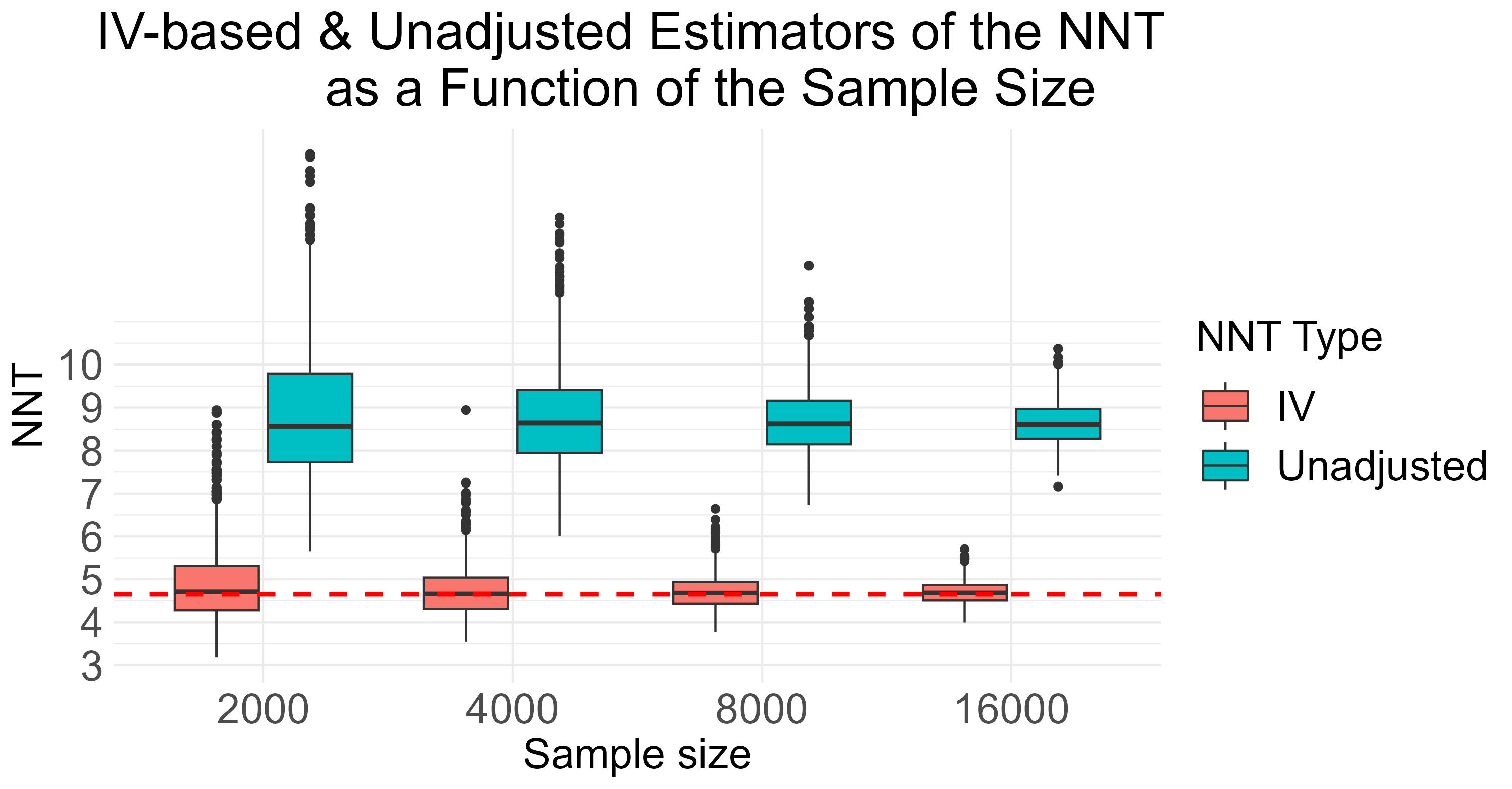
(a) Double logit model. True NNT$=4.65$.

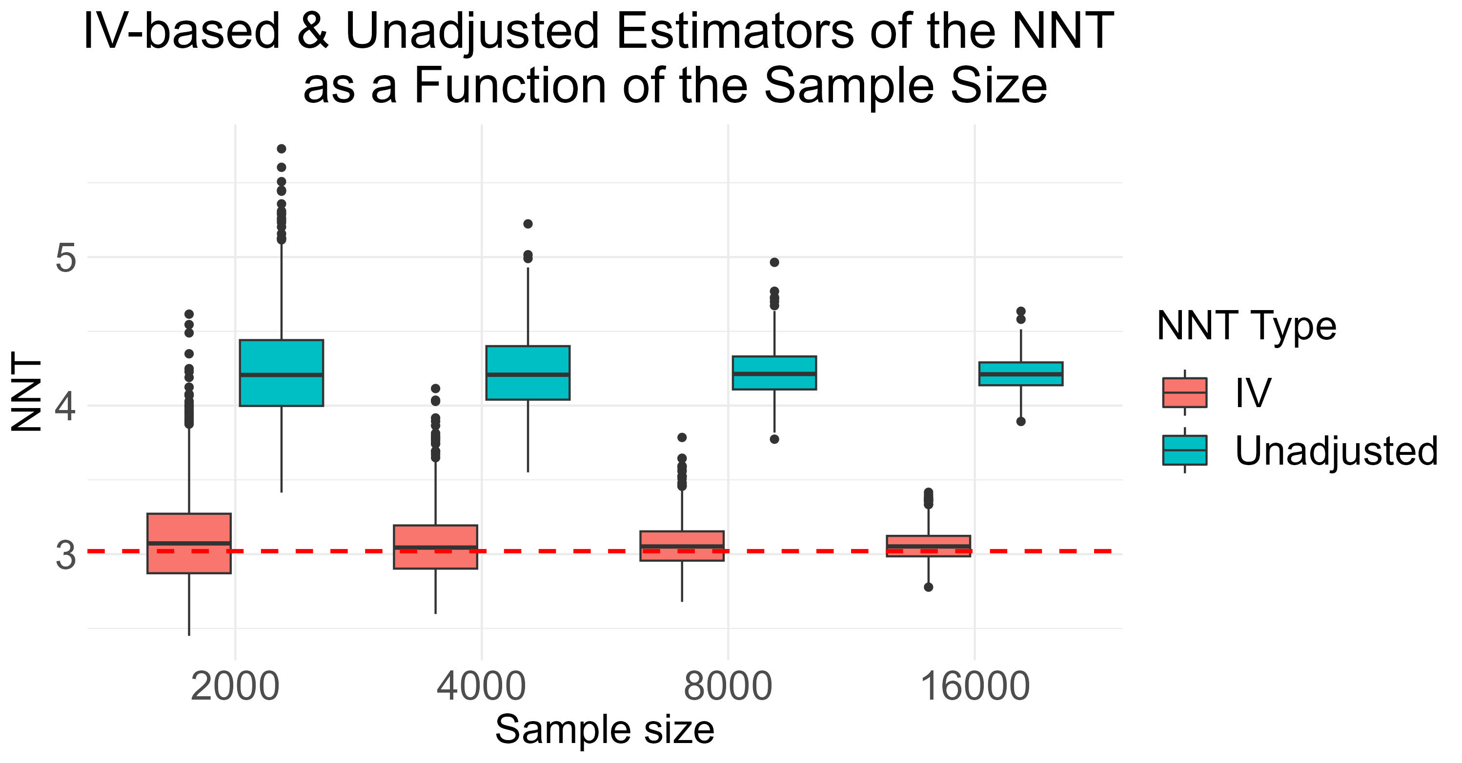
(b) Double probit model. True NNT$=3.02$.

Figure 3: Logit and probit models example: Binary outcome with logit and probit causal models, respectively. The true causal parameters for both models are $\psi=(1,1.5)^{T}$. The true populationwise NNTs are $4.65$, and $3.02$, respectively. The red boxplots denote the IV-based estimators of the NNT, which are based on G-estimators of $\psi$. The blue boxplots denote the unadjusted estimators of the populationwise NNT. The red dashed line denotes the true NNT value for each model. The calculations were repeated $m=1000$ times for four different sample sizes: $n=2000,4000,8000,16000$. For both models, the marginal $P(A=1)=0.6$, $\pi_{Z}=0.5$, $\gamma=(-0.83,3)^{T}$ and the marginal probability of the outcome is $P(I=1)=0.3$.

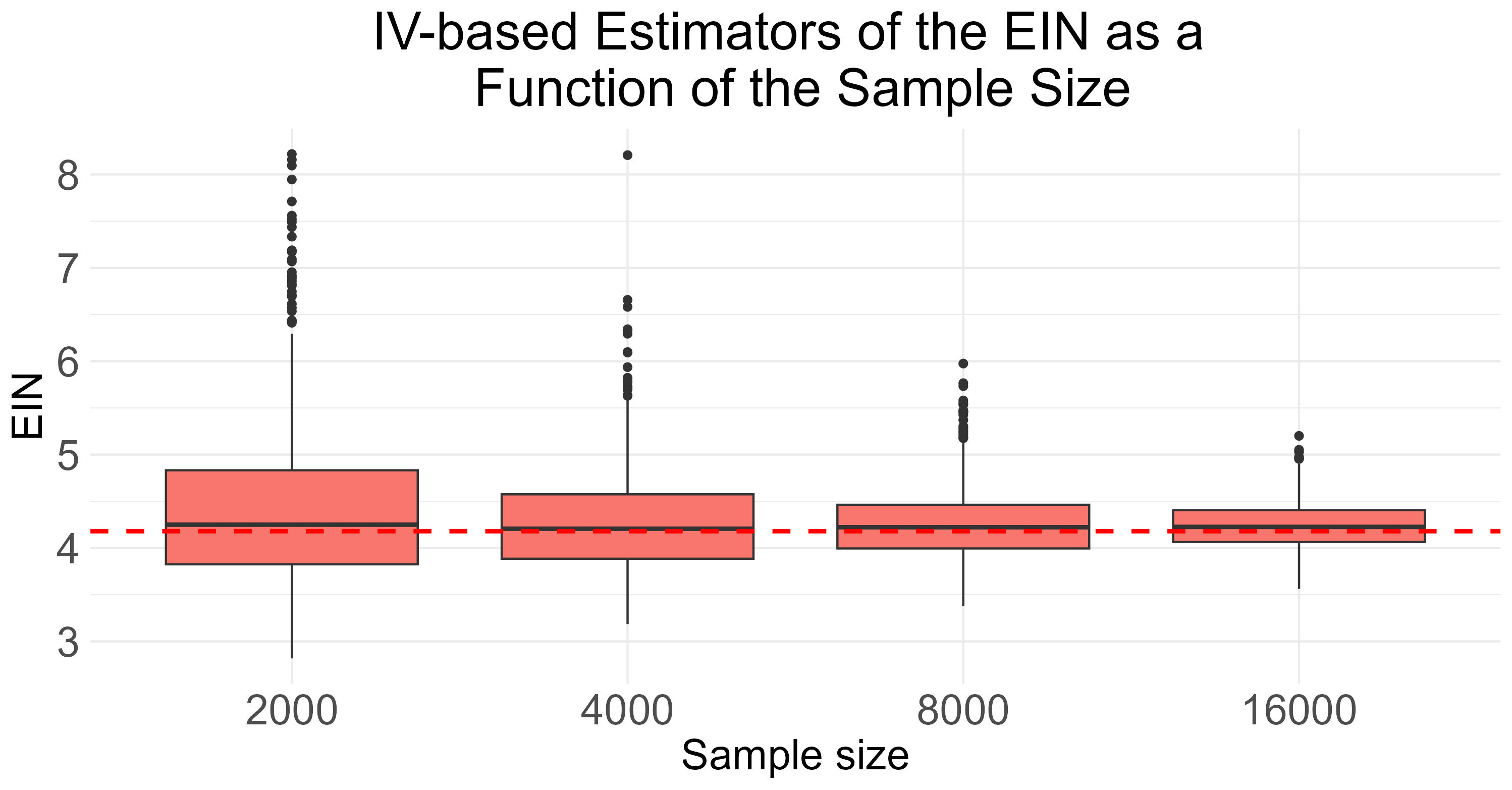
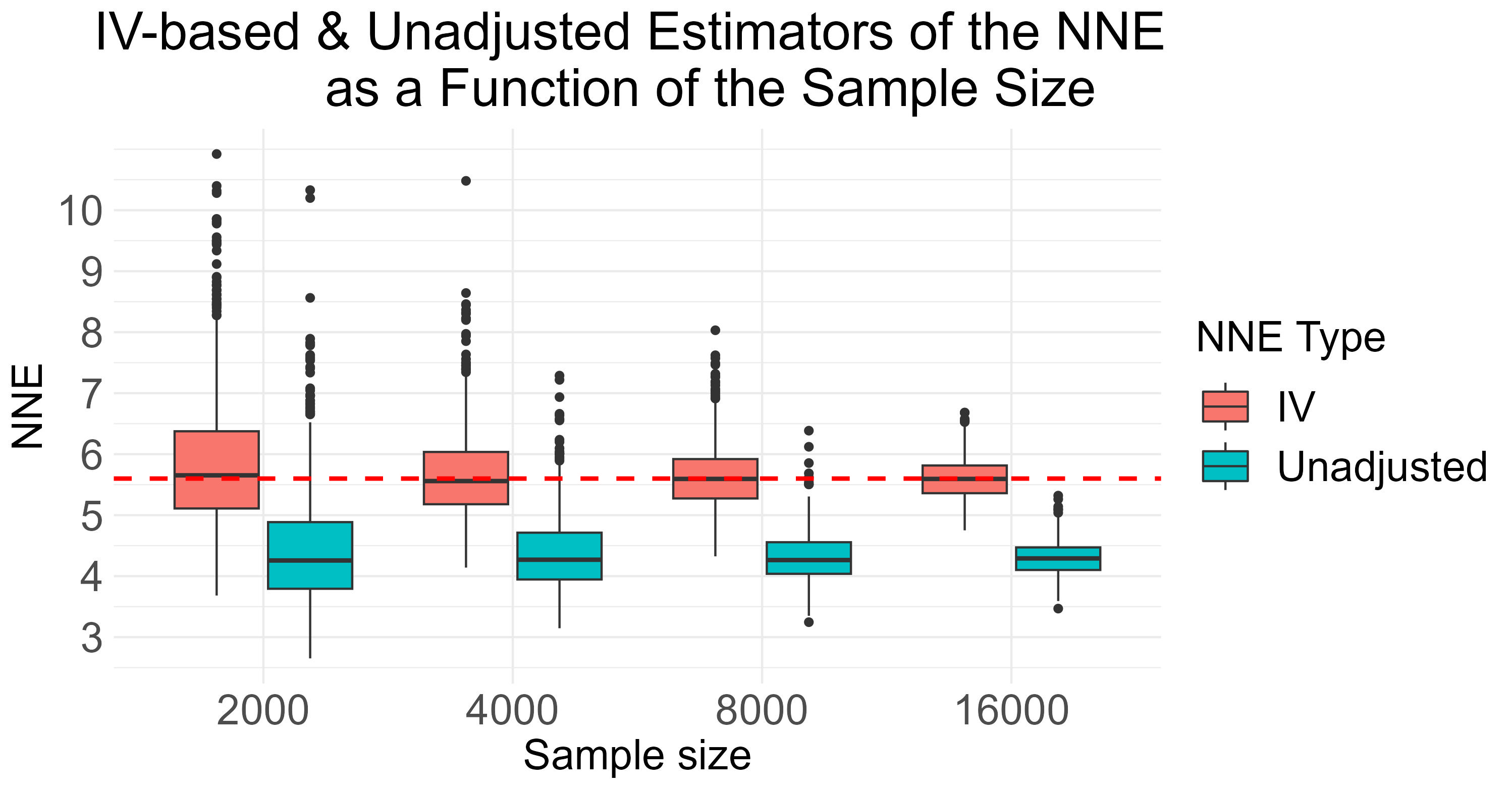
(a) Double logit model. True EIN$=4.18$.

(b) Double probit model. True EIN$=2.81$.

Figure 4: Double logit and probit models example: Binary outcome with logit and probit causal models, respectively. The causal parameters are $\psi=(1,1.5)^{T}$. The true EINs are $4.18$ and $2.81$, respectively. The red boxplots denote the IV-based estimators of the EIN, which are based on G-estimators of $\psi$. The unadjusted estimators of the EIN were infinitely large (the estimated probabilities of benefit were negative before the application of the function $g$ (2)); therefore, they were omitted from the graph. The red dashed line denotes the true EIN value in each model. The calculations were repeated $m=1000$ times for four different sample sizes: $n=2000,4000,8000,16000$. For both models, the marginal $P(A=1)=0.6$, $\pi_{Z}=0.5$, $\gamma=(-0.83,3)^{T}$ and the marginal probability of the outcome is $P(I=1)=0.3$.

(a) Double logit model. True NNE$=5.60$.

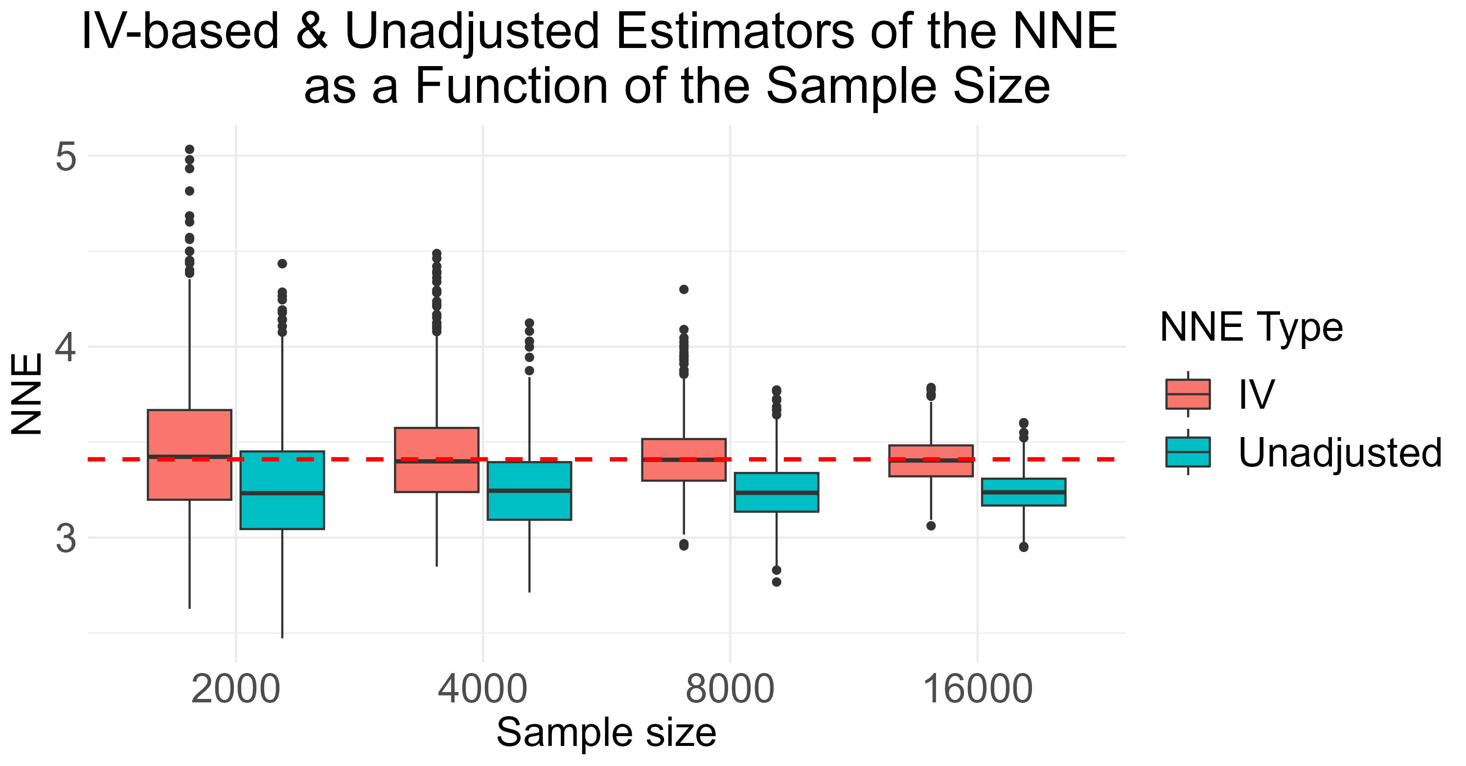
(b) Double probit model. True NNE$=3.41$.

Figure 5: Double logit and probit models example: Binary outcome with logit and probit causal models, respectively. The true causal parameters for both models are $\psi=(1,1.5)^{T}$. The true populationwise NNEs are $5.60$, and $3.41$, respectively. The red boxplots denote the IV-based estimators of the NNE, which are based on G-estimators of $\psi$. The blue boxplots denote the unadjusted estimators of the NNE. The red dashed line denotes the true NNE value for each model. The calculations were repeated $m=1000$ times for four different sample sizes: $n=2000,4000,8000,16000$. For both models, the marginal $P(A=1)=0.6$, $\pi_{Z}=0.5$, $\gamma=(-0.83,3)^{T}$ and the marginal probability of the outcome is $P(I=1)=0.3$.

5.2 Simulation summary

Graphical summary of the estimators’ behavior as a function of the sample size $n$ can be found in Figures 3,  4, and 5. Figure 3 illustrate the behavior of the populationwise NNTs estimators, Figure 4 illustrate the behavior of the EINs estimators, and Figure 5 illustrate the behavior of the NNEs estimators for the double logit and probit models, respectively. One can observe that for the populationwise NNT, the unadjusted estimators are biased upwards, whereas for the EIN and NNE are biased downwards. For the EIN, the bias is severe and produces infinitely large estimators, while for the NNE, the bias is rather small. For all indices, the estimators of the probit model are less stable (have larger variance). Table 1 presents the coverage rates of the $95\%$-level CI for the marginal EIN, NNE, and NNT in double logit and probit models as a function of the sample size $n$. The empirical coverage rates are close to the nominal $95\%$ for the double logit model. For the double probit model, there is a certain overshooting for EIN and NNT indices, for $n=2000$. This phenomenon can be attributed to the higher variability of the estimators, compared to the logit model, for the smaller sample sizes. In summary, in the presence of omitted confounders, the novel estimation method produces consistent estimators and reliable CIs for the true EIN, NNE, and NNT.

Model		logit			probit
$n$	EIN	NNE	NNT	EIN	NNE	NNT
2000	0.957	0.937	0.941	0.993	0.945	0.980
4000	0.953	0.946	0.948	0.977	0.941	0.974
8000	0.954	0.938	0.946	0.966	0.939	0.960
16000	0.955	0.937	0.952	0.923	0.939	0.939

Table 1: Double logit and probit models examples: Empirical coverage rates of the sandwich-matrix-based $95\%$-level CIs for the marginal EIN, NNE, and NNT, as a function of the sample size $n=2000,4000,8000,16000$. The number of iterations for each sample size is $m=1000$.

6 Real world data example

To illustrate our novel estimation method in a real-world scenario, we use the vitamin D data available in the ivtools R-package. These publicly available data are a modified version of the original data from a cohort[35] study on vitamin D status causal effect on mortality rates previously used by Sjölander & Martinussen.[33] Vitamin D deficiency has been linked with several lethal conditions such as diabetes, cancer, and cardiovascular diseases. However, vitamin D status is also associated with several behavioral and environmental factors, such as season and smoking habits, that may result in biased estimators when using standard statistical analyses to estimate causal effects.

Mendelian randomization[36, 37] is a method whose principles were introduced originally by Katan[38] in a medical context. Subsequently, Youngmen et al.[39] introduced this method in the context of epidemiological studies and also coined the aforementioned term. The underlying principle of the method is to use genotypes as IVs to estimate the causal effect of phenotype on disease-related outcomes. The population distribution of genetic variants is assumed to be independent of behavioral and environmental factors that usually confound the effect of exposure on the outcome. The process governing the distribution of genetic variants in the population resembles the randomization mechanism in RCTs.

In our example, the phenotype is vitamin D baseline status, the outcome is survival at the follow-up endpoint, and the genotype is mutations in the filaggrin gene. These mutations are associated with a higher serum vitamin D concentration. The prevalence of this mutation is estimated to be $8\%-10\%$ in the northern European population. We used the modified version of data obtained in the Monica10 population-based study. This is a $10$-years follow-up study started in 1982-1984 that initially included an examination of $3,785$ individuals of Danish origin. In the follow-up study of 1993-1994, the participation rate was about $70\%$. It resulted in data that contained a total of $2,656$ participants, where $2,571$ were also available in the modified data after the removal of cases that had missing information on filaggrin and or on vitamin D status.[40, 35] These data consisted of $5$ variables: age (at baseline), filaggrin (a binary indicator of whether filaggrin mutations are present), vitd (vitamin D level at baseline as was assessed by serum 25-hydroxyvitamin D 25-OH-D(nmol/L) concentration on serum lipids), time (follow-up time), and death (an indicator of whether the subject died during follow-up).

This analysis considers only the necessary variables for the required estimators. We use the binary indicator of survival at the follow-up endpoint as the outcome $I$ and the binary indicator of the presence of the filaggrin gene mutation as the IV $Z$. For the binary exposure $A$, the vitamin D status at baseline (vitd) was dichotomized at a threshold serum level of $30$ ng/mL, defined as the bottom end of the acceptable range of vitamin D for skeletal health.[41] Values higher (or equal) $30$ were defined as $1$ to indicate an exposure, and $0$ otherwise to indicate non-exposure. The estimated models were the double logit and the double probit models. In particular, the explicit form of the assumed GSMM are as presented in eq. (13) and eq. (33), and the form of the assumed association models for the observed outcome are as presented in eq. (14), and eq. (34), for the logit and probit models, respectively. Namely, for each model, the core estimands are two causal parameters $\psi=(\psi_{0},\psi_{1})^{T}$, four association model parameters $\beta_{I}=(\beta_{0},\beta_{1},\beta_{2},\beta_{3})^{T}$, and one IV model parameter $\pi_{Z}$. The indices of interest (EIN, NNE, and NNT) are functions of these parameters. The populationwise NNT in such a case is the average number of randomly drawn individuals whose vitamin D level needs to be increased to the normal range (above $30$ ng/mL) to prevent additional death during the follow-up period. Analogically, the NNE is the average number of randomly drawn individuals from the unexposed group whose vitamin D level needs to be elevated to the normal range to prevent one additional death during the follow-up period. The EIN is defined similarly to NNE for the exposed group. The marginal probability $\pi_{Z}$ was estimated using the sample mean of the filaggrin gene mutation indicator. We used both the double logit and double probit models to estimate the EIN, NNE, and NNT.

The EIN point estimators with the corresponding $95\%$-level CI were $1.53$ $[1.16,1.91]$, and $1.51$ $[1.12,1.90]$, for the double logit and double probit models, respectively. There was no solution for $\psi_{0}$ under these two models, therefore, we were unable to compute the corresponding NNE and NNT estimators. Namely, according to the results obtained from the novel estimation method, increasing the vitamin D level to the normal range in the exposed group (i.e., the group with normal vitamin D levels) is highly effective for preventing fatal outcomes. The absence of a solution for $\psi_{0}$ can result from various reasons, where the most probable is insufficient data. Namely, the unexposed group constitutes only about $7\%$ of the cohort, combined with a low filaggrin gene mutation prevalence in this group ($<3\%$), which may result in insufficient sample size for reliable estimation of $\psi_{0}$. Another reason may be the misspecification of either the association (outcome) or the causal model for the unexposed group. Yet since most of the observations ($93\%$) are from the exposed group, assuming that the true NNE is reasonably small, we can deduce that the NNT’s true value is close to the EIN value. Namely, increasing the vitamin D level to the normal range in the whole population is also expected to be highly effective for fatal outcomes prevention. The source code of this analysis is available on the author’s GitHub repository.

7 Summary and Conclusions

In observational studies, the exposed group characteristics may substantially differ from the unexposed. To address this issue, groupwise efficacy indices were defined: the EIN for the exposed group and the NNE for the unexposed. In such studies, the group allocation is typically affected by confounders. In many studies, the measured confounders cannot be assumed sufficient for confounding control. Therefore, using the available estimation methods to estimate the EIN, NNE, or NNT will result in inconsistent estimators. Using Rubin’s potential outcomes framework, this study explicitly defines the NNT and its derived indices, EIN and NNE, as causal measures. Then, we introduce a novel method that uses IVs to estimate the three aforementioned indices in observational studies where the omission of unmeasured confounders cannot be ruled out. We present two analytical examples – double logit and double probit models. Next, a corresponding simulation study is conducted. The simulation study illustrates the improved performance of the new estimation method compared to the available methods in terms of consistency and CIs coverage rates. Finally, a real-world example based on a study of vitamin D deficiency effects on mortality rates is presented. In this example, we evaluate the efficacy of increasing vitamin D to normal levels to prevent fatal outcomes. The new estimator suggests that increasing vitamin D level above 30 ng/mL among the exposed group is highly efficient in preventing death.

This study is not without limitations. In the examined models, we considered only binary observed outcomes. However, in many studies, the observed outcome is non-binary, and the dichotomization is performed using a certain threshold, as we did in the vitamin D example. This practice has disadvantages - such dichotomization results in loss of Fisher information and, therefore, a decrease in statistical power.[28, 29] Although the illustrated theoretical setup is non-parametric, the examined causal and association models are semi-parametric. These types of models are attractive since they simplify the estimation procedure. However, such models are sensitive to model misspecification as we need to specify three different models; (1) one for the instrumental variable, (2) one for the association (outcome) model, and (3) one for the GSMM. This results in three sets of parameters that need to be estimated and three different models that can be misspecified. Therefore, non-parametric estimation might serve as a possible direction for future research. Another limitation is the reliance of the estimation method on the availability of a valid IV. Such a variable is not always available, and even when we can obtain an IV, its validity relies partially on subject matter knowledge. Therefore, another possible research direction is a sensitivity analysis of the estimators to violations of valid IV assumptions.[42] Additional possible limitation is the plausability of the monotonicity assumption. In some scenarious this assumption is satisfied by the study design or the DGP;[21] in other scenarios, its status is undetermined or violated. In a recent study,[43] Mueller and Pearl demonstrated how monotonicity can be validated or refuted from observational data. Namely, it is generally a testable assumption. Notably, our methodology is applicable even if the monotonicity assumption is violated. In such a case, the primary distinction lies in the interpretation of the estimates. Namely, the EIN, NNE, and NNT are then estimated by the reciprocal of the ATE in the corresponding group, which differs from the (conditional) exposure benefit probability. Therefore, the estimands are not informative on the individual level and can be interpreted only as population average effects.

The main contribution of this study is by providing explicit causal formulation of the EIN, NNE, and NNT and a comprehensive theoretical framework for their point and interval estimation in observational studies with unmeasured confounders. Future research direction may focus either on applications or extensions of the novel method to new domains.

Appendix A APPENDIX

A.1 Proof of unbiasedness of the G-estimators estimating equations

Without the loss of generality, we present the proof for the exposed group, $a=1$. The proof for the unexposed group can be readily obtained using analogical steps for $a=0$. Assume a double $\xi$ model, where $\xi$ is a general link function for the GSMM (5) and the association model $\xi([E|Z,L,A;\beta_{I}])$. Let the estimating equation for the G-estimator of $\psi_{1}$ be as defined in eq. (19). Therefore,

$$E[D_{1}(Z,L;\pi_{Z})h(1;Z,L,\beta_{I},\psi_{1})] =E[D_{1}(Z,L;\pi_{Z})\xi^{-1}\left(\xi(E[I|Z,L,A=1;\beta_{I}])-m_{1}^{T}(L)\psi_{1}\right)]$$ (29)

$$=E[D_{1}(Z,L;\pi_{Z})\xi^{-1}\left(\xi(E[I_{1}|Z,L,A=1;\beta_{I}])-m_{1}^{T}(L)\psi_{1}\right)]$$ (30)

$$=E[D_{1}(Z,L;\pi_{Z})\xi^{-1}\left(\xi(E[I_{0}|Z,L,A=1;\beta_{I}])\right)]$$

$$=E[D_{1}(Z,L;\pi_{Z})E[I_{0}|Z,L,A=1]]$$

$$=E[E[D_{1}(Z,L;\pi_{Z})I_{0}|Z,L,A=1]]$$ (31)

$$=E[D_{1}(Z,L;\pi_{Z})I_{0}]$$ (32)

$$=0.$$

Eq. (29) is a direct consequence of the assumed GSMM structure in eq. (5). Eq. (30) stems from the consistency assumption.[30] Eq. (31) holds since the potential outcome $I_{0}$ is independent of the observed allocation $A$. The last step in eq. (32) stems from the validity of the IV. Namely, the estimating equations are unbiased as long as the IV $Z$ satisfies conditions of a valid IV, i.e., $I_{0}\rotatebox[origin={c}]{90.0}{$\models$}Z|L$.

A.2 The double probit model example

Assume a binary outcome $I\in\{0,1\}$, a binary exposure $A\in\{0,1\}$, and a binary instrument $Z\in\{0,1\}$. Assume there are no measured confounders, i.e., $L=\emptyset$ and $m(L)=1$. For the probit link function $\xi$, we define the GSMM (5) as

$$\Phi^{-1}\left(E[I_{1}=1|Z,A=a]\right)-\Phi^{-1}\left(E[I_{0}=1|Z,A=a]\right)=\psi_{a},\quad a\in\{0,1\},$$ (33)

where $\Phi^{-1}(x)$ is the inverse of the standard normal random variable’s cumulative distribution function $\Phi(x)=\int_{-\infty}^{x}(2\pi)^{-1/2}\exp\{-s^{2}/2\}ds$. Additionally, assume the following saturated probit model for the observed outcome

$$\Phi^{-1}\left(E[I|Z,A;\beta_{I}]\right)=\beta_{0}+\beta_{1}A+\beta_{2}Z+\beta_{3}ZA.$$ (34)

Using the GSMM and the probit association model, we can express explicitly the general conditional exposure benefit probability (12) as a function of $\beta_{I}$ and $\psi$

$$p_{b}(Z,A,\beta_{I},\psi) =\Phi\left(\beta_{0}+\beta_{1}A+\beta_{2}Z+\beta_{3}ZA+\psi_{0}(1-A))\right)$$ (35)

$$-\Phi\left(\beta_{0}+\beta_{1}A+\beta_{2}Z+\beta_{3}ZA-\psi_{1}A\right).$$

To compute the populationwise NNT, we apply the function $g$ to the marginal exposure benefit probability $p_{b}=E[p_{b}(Z,A,\beta_{I},\psi)]$ (9), i.e., $\text{NNT}=g(p_{b})$. If we set $A$ to $0$ in eq. (35) we obtain the conditional exposure benefit probability (10) for the unexposed $a=0$ as a function of $\beta_{I}$ and $\psi_{0}$

$$p_{b}(0;Z,\beta_{I},\psi_{0})=\Phi(\beta_{0}+\beta_{2}Z+\psi_{0})-\Phi(\beta_{0}+\beta_{2}Z),$$ (36)

To compute the NNE, we apply the function $g$ to the marginal exposure benefit probability for the unexposed $p_{b}(0)=E[p_{b}(0;Z,\beta_{I},\psi_{0})|A=0]$ (11), i.e., $\text{NNE}=g(p_{b}(0))$. Analogically, for the conditional exposure benefit probability (10) for the exposed $a=1$, we set $A$ to $1$ in eq. (15)

$$p_{b}(1;Z,\beta_{I},\psi_{1}) =\Phi(\beta_{0}+\beta_{1}+\beta_{2}Z+\beta_{3}Z)-\Phi(\beta_{0}+\beta_{1}+\beta_{2}Z+\beta_{3}Z-\psi_{1}).$$ (37)

To compute the EIN, we apply the function $g$ to the marginal exposure benefit probability for the exposed $p_{b}(1)=E[p_{b}(1;Z,\beta_{I},\psi_{1})|A=1]$ (11), i.e., $\text{EIN}=g(p_{b}(1))$.

A.3 Explicit form of valid IV conditions

A.3.1 The double logit model

Let the GSMM be defined as in eq. (13), and the marginal distribution of the IV $Z$ and the conditional distribution of the exposure $A$ are as specified in (26). For a double logit model, the explicit form of eq. (28) for the potential outcome $I_{0}$ is

$$\text{expit}(\beta_{0}+\beta_{2})(1-\text{expit}(\gamma_{0}+\gamma_{1}))+\text{expit}(\beta_{0}+\beta_{1}+\beta_{2}+\beta_{3}-\psi_{1})\text{expit}(\gamma_{0}+\gamma_{1})$$

$$=\text{expit}(\beta_{0})(1-\text{expit}(\gamma_{0}))+\text{expit}(\beta_{0}+\beta_{1}-\psi_{1})\text{expit}(\gamma_{0}),$$ (38)

and for the potential outcome $I_{1}$ is

$$\text{expit}(\beta_{0}+\beta_{2}+\psi_{0})(1-\text{expit}(\gamma_{0}+\gamma_{1}))+\text{expit}(\beta_{0}+\beta_{1}+\beta_{2}+\beta_{3})\text{expit}(\gamma_{0}+\gamma_{1})$$

$$=\text{expit}(\beta_{0}+\psi_{0})(1-\text{expit}(\gamma_{0}))+\text{expit}(\beta_{0}+\beta_{1})\text{expit}(\gamma_{0}).$$ (39)

A.3.2 The double probit model

Let the GSMM be defined as in eq. (33), and the function $\xi$ be the probit $\Phi$ function. The explicit forms of the exposure benefit probabilities are given in eq. (36) and (37). The explicit forms of eq. (28) for the potential outcomes $I_{0}$ and $I_{1}$ are obtained by replacing the expit function with the probit function $\Phi$ in equations (A.3.1) and (A.3.1), respectively.

A.4 Simulation study, Step 2: Estimation

This subsection presents the explicit form of the vector-valued function $\mathbf{Q}(Z,A;\theta)$ components. The vector of unbiased estimating functions (22) of $\beta_{I}$ and $\pi_{Z}$ consists of the score functions of the association model (27) and the binary instrument model (26), namely,

$$\mathbf{S}(Z,A;\beta_{I},\pi_{Z})=\begin{pmatrix}(I-\xi^{-1}(\beta_{0}+\beta_{1}A+\beta_{2}Z+\beta_{3}AZ))\\ (I-\xi^{-1}(\beta_{0}+\beta_{1}A+\beta_{2}Z+\beta_{3}AZ))A\\ (I-\xi^{-1}(\beta_{0}+\beta_{1}A+\beta_{2}Z+\beta_{3}AZ))Z\\ (I-\xi^{-1}(\beta_{0}+\beta_{1}A+\beta_{2}Z+\beta_{3}AZ))AZ\\ (Z-\pi_{Z})\end{pmatrix}.$$

The vector-valued function $\mathbf{Dh}(Z,A;\beta_{I},\pi_{Z},\psi)$ as in eq. (19) of the two estimating functions for the causal parameters $\psi$ is

$$\mathbf{Dh}(Z,A;\beta_{I},\pi_{Z},\psi)=\begin{pmatrix}(Z-\pi_{Z})\xi^{-1}\left(\beta_{0}+\beta_{1}A+\beta_{2}Z+\beta_{3}AZ+\psi_{0}(1-A)\right)\\ (Z-\pi_{Z})\xi^{-1}\left(\beta_{0}+\beta_{1}A+\beta_{2}Z+\beta_{3}AZ-\psi_{1}A\right)\ \end{pmatrix}.$$

The vector-valued function $\mathbf{p}\left(Z,L,A;\beta_{I},\psi,p_{b}(0),p_{b}(1),p_{b}\right)$ as in eq. (23) consists of the three estimating equations for the exposure benefit probabilities

$$\mathbf{p}\left(Z,L,A;\beta_{I},\psi,p_{b}(0),p_{b}(1),p_{b}\right)$$

$$=\begin{pmatrix}\left(\xi^{-1}\left(\beta_{0}+\beta_{2}Z+\psi_{0}\right)-\xi^{-1}\left(\beta_{0}+\beta_{2}Z\right)-p(0)\right)(1-A)\\ \left(\xi^{-1}\left(\beta_{0}+\beta_{1}+\beta_{2}Z+\beta_{3}Z\right)-\xi^{-1}\left(\beta_{0}+\beta_{1}+\beta_{2}Z+\beta_{3}Z-\psi_{1}\right)-p(1)\right)A\\ \xi^{-1}\left(\beta_{0}+\beta_{1}A+\beta_{2}Z+\beta_{3}AZ+\psi_{0}(1-A)\right)-\xi^{-1}\left(\beta_{0}+\beta_{1}A+\beta_{2}Z+\beta_{3}AZ-\psi_{1}A\right)-p_{b}\\ \end{pmatrix}.$$

In all components of the estimating function $\mathbf{Q}(Z,A;\theta)$, $\xi^{-1}$ is the expit and the inverse probit $\Phi^{-1}$ functions for the double logit and double probit models, respectively. Notably, the vector valued function $\mathbf{g}\left(p_{b}(0),p_{b}(1),p_{b},\text{NNE, EIN, NNT}\right)$ is independent of the data, and thus its form remains the same as in its definition in (24).

References

- [1] Newcombe RG. Confidence intervals for proportions and related measures of effect size. CRC press; 2012.
- [2] Vancak V, Goldberg Y, Levine SZ. Guidelines to understand and compute the number needed to treat. BMJ Ment Health. 2021;24(4):131-6.
- [3] Lee TY, Kuo S, Yang CY, Ou HT. Cost-effectiveness of long-acting insulin analogues vs intermediate/long-acting human insulin for type 1 diabetes: A population-based cohort followed over 10 years. Brit J Clin Pharmaco. 2020;86(5):852-60.
- [4] Verbeek JG, Atema V, Mewes JC, et al. Cost-utility, cost-effectiveness, and budget impact of Internet-based cognitive behavioral therapy for breast cancer survivors with treatment-induced menopausal symptoms. Breast cancer Res Tr. 2019;178(3):573-85.
- [5] da Costa BR, Rutjes AW, Johnston BC, et al. Methods to convert continuous outcomes into odds ratios of treatment response and numbers needed to treat: meta-epidemiological study. Int J Epidemiol. 2012;41(5):1445-59.
- [6] Mendes D, Alves C, Batel-Marques F. Number needed to treat (NNT) in clinical literature: an appraisal. BMC Med. 2017;15(1):1-13.
- [7] Bender R, Blettner M. Calculating the “number needed to be exposed” with adjustment for confounding variables in epidemiological studies. J Clin Epidemiol. 2002;55(5):525-30.
- [8] Laupacis A, Sackett DL, Roberts RS. An assessment of clinically useful measures of the consequences of treatment. New Engl J Med. 1988;318(26):1728-33.
- [9] Kristiansen IS, Gyrd-Hansen D, Nexøe J, et al. Number needed to treat: easily understood and intuitively meaningful?: theoretical considerations and a randomized trial. J Clin Epidemiol. 2002;55(9):888-92.
- [10] Bender R, Kuss O, Hildebrandt M, Gehrmann U. Estimating adjusted NNT measures in logistic regression analysis. Stat Med. 2007;26(30):5586-95.
- [11] Bender R, Vervölgyi V. Estimating adjusted NNTs in randomised controlled trials with binary outcomes: a simulation study. Contem Clin Trials. 2010;31(5):498-505.
- [12] Sjölander A. Estimation of causal effect measures with the R-package stdReg. Eur J Epidemiol. 2018;33(9):847-58.
- [13] Mueller S, Pearl J. Personalized decision making–A conceptual introduction. J Causal Inference. 2023;11(1):20220050.
- [14] Vancak V, Goldberg Y, Levine SZ. The number needed to treat adjusted for explanatory variables in regression and survival analysis: Theory and application. Stat Med. 2022;41(17):3299-320.
- [15] Rubin DB. Causal inference using potential outcomes: Design, modeling, decisions. J Am Stat Assoc. 2005;100(469):322-31.
- [16] Pearl J. Probabilities of causation: three counterfactual interpretations and their identification. In: Probabilistic and Causal Inference: The Works of Judea Pearl; 2022. p. 317-72.
- [17] Schulzer M, Mancini GJ. ‘Unqualified Success’ and ‘Unmitigated Failure’Number-Needed-to-Treat-Related Concepts for Assessing Treatment Efficacy in the Presence of Treatment-Induced Adverse Events. Int J Epidemiol. 1996;25(4):704-12.
- [18] Laubender RP, Bender R. Estimating adjusted risk difference (RD) and number needed to treat (NNT) measures in the Cox regression model. Stat Med. 2010;29(7-8):851-9.
- [19] Walter SD. Number needed to treat (NNT): estimation of a measure of clinical benefit. Stat Med. 2001;20(24):3947-62.
- [20] Angrist JD, Imbens GW, Rubin DB. Identification of causal effects using instrumental variables. J Am Stat Assoc. 1996;91(434):444-55.
- [21] Angrist JD, Imbens GW. Two-stage least squares estimation of average causal effects in models with variable treatment intensity. J Am Stat Assoc. 1995;90(430):431-42.
- [22] Grieve AP. The number needed to treat: a useful clinical measure or a case of the Emperor’s new clothes? Pharm Stat. 2003;2(2):87-102.
- [23] Hutton JL. Number needed to treat: properties and problems. J Roy Stat Soc A Stat. 2000;163(3):381-402.
- [24] Snapinn S, Jiang Q. On the clinical meaningfulness of a treatment’s effect on a time-to-event variable. Stat Med. 2011;30(19):2341-8.
- [25] Sønbø Kristiansen I, Gyrd-Hansen D. Cost-effectiveness analysis based on the number-needed-to-treat: common sense or non-sense? Health Econ. 2004;13(1):9-19.
- [26] Vancak V, Goldberg Y, Levine SZ. Systematic analysis of the number needed to treat. Stat Methods Med Res. 2020;29(9):2393-410.
- [27] Holland PW. Statistics and causal inference. J Am Stat Assoc. 1986;81(396):945-60.
- [28] Senn S. Disappointing dichotomies. Pharm Stat. 2003;2(4):239-40.
- [29] Fedorov V, Mannino F, Zhang R. Consequences of dichotomization. Pharm Stat. 2009;8(1):50-61.
- [30] Didelez V, Meng S, Sheehan NA. Assumptions of IV methods for observational epidemiology. Stat Sci. 2010;25(1):22-40.
- [31] Robins JM. Correcting for non-compliance in randomized trials using structural nested mean models. Commu Stat Theory M. 1994;23(8):2379-412.
- [32] Stefanski LA, Boos DD. The calculus of M-estimation. Am Stat. 2002;56(1):29-38.
- [33] Sjölander A, Martinussen T. Instrumental variable estimation with the R package ivtools. Epidemiol Methods. 2019;8(1).
- [34] Borchers HW, Borchers MHW. Package ‘pracma’. accessed on. 2022;4.
- [35] Skaaby T, Husemoen LLN, Pisinger C, et al. Vitamin D status and incident cardiovascular disease and all-cause mortality: a general population study. Endocrine. 2013;43(3):618-25.
- [36] Davey Smith G, Ebrahim S. ‘Mendelian randomization’: can genetic epidemiology contribute to understanding environmental determinants of disease? Int J Epidemiol. 2003;32(1):1-22.
- [37] Smith GD, Ebrahim S. Mendelian randomization: prospects, potentials, and limitations. Int J Epidemiol. 2004;33(1):30-42.
- [38] Katan MB. Apoupoprotein E isoforms, serum cholesterol, and cancer. Lancet. 1986;327(8479):507-8.
- [39] Youngman L, Keavney B, Palmer A, et al. Plasma fibrinogen and fibrinogen genotypes in 4685 cases of myocardial infarction and in 6002 controls: Test of causality by” Mendelian randomisation”. Circulation. 2000;102(18).
- [40] Martinussen T, Nørbo Sørensen D, Vansteelandt S. Instrumental variables estimation under a structural Cox model. Biostatistics. 2019;20(1):65-79.
- [41] Heaney RP, Holick MF. Why the IOM recommendations for vitamin D are deficient. J Bone Miner Res. 2011;26(3):455-7.
- [42] Vancak V, Sjölander A. Sensitivity Analysis of G-estimators to Invalid Instrumental Variables. to appear in Stat Med. 2023.
- [43] Mueller S, Pearl J. Monotonicity: Detection, Refutation, and Ramification. 2023.