Confined granular gases under the influence of vibrating walls

Abstract

The dynamics of a system composed of inelastic hard spheres or disks that are confined between two parallel vertically vibrating walls is studied (the vertical direction is defined as the direction perpendicular to the walls). The distance between the two walls is supposed to be larger than twice the diameter of the particles so that the particles can pass over each other, but still much smaller than the dimensions of the walls. Hence, the system can be considered to be quasi-two-dimensional (quasi-one-dimensional) in the hard spheres (disks) case. For dilute systems, a closed evolution equation for the one-particle distribution function is formulated that takes into account the effects of the confinement. Assuming the system is spatially homogeneous, the kinetic equation is solved approximating the distribution function by a two-temperatures (horizontal and vertical) gaussian distribution. The obtained evolution equations for the partial temperatures are solved, finding a very good agreement with Molecular Dynamics simulation results for a wide range of the parameters (inelasticity, height and density) for states whose projection over a plane parallel to the walls is homogeneous. In the stationary state, where the energy lost in collisions is compensated by the energy injected by the walls, the pressure tensor in the horizontal direction is analyzed and its relation with an instability of the homogenous state observed in the simulations is discussed.

Confined gas

Authors here

I Introduction

Granular gases are systems composed of macroscopic particles which do not conserve kinetic energy when they collide. As a consequence, they are intrinsically out of equilibrium and have a very rich phenomenology g03 ; at06 ; brilliantov ; garzo19 , so they can be considered as a proving ground for nonequilibrium statistical mechanics. In the last years, many studies have been focused on a thin vertical granular system that is vertically vibrating peu02 ; ou05 ; mvprkeu05 ; cms12 ; nrtms14 ; cms15 ; gs18 . The reason is that, for a wide class of initial conditions, when the system is observed from above (or below), a homogeneous stationary state is reached in the long time limit. In this state, the energy lost in collisions is compensated by the energy injected by the walls. The fact that the system is out of equilibrium and, still, spatially homogeneous, is very peculiar. In effect, in molecular systems the out of equilibrium character is usually linked to the presence of gradients. For granular systems, this is also the case as can be seen from the hydrodynamic equations bdks98 . For this particular setup, the gradients appear in the vertical direction and can be neglected if the height of the system is small enough. Interestingly, when varying the values of some parameters, as the amplitude of the oscillations or the total density, the system reaches a different state in which a solid-like phase is surrounded by a hotter dilute gas. The origin of this phase transition has been extensively studied (see, for example, the reviews mvprkeu05 ; gs18 ) being the ingredient that triggers the instability a negative compressibility in the horizontal direction brs13 . To be precise, the horizontal stationary pressure tensor is a monotonically decreasing function of the mean density. Then, if a dense region is spontaneously developed, it has associated a lower pressure attracting more particles and triggering the instability.

Many of the above studies have concentrated in the ultra-confined case in which the height of the system is smaller than twice the diameter of the particles, in such a way that particles can not jump over each other and the system can be considered quasi-two-dimensional (Q2D). One of the simplest models used for the theoretical studies for this Q2D system is an ensemble of inelastic spheres confined between two flat planes that inject energy into the system in the vertical direction mgb19 ; mgb19b ; mgb22 . Gravity is not consider and by vertical direction we mean the direction perpendicular to the walls. The energy injection is the corresponding to an elastic wall that vibrates sinusoidally with amplitude $A$ and frequency $\omega$ in the double limit $A\to 0$, $\omega\to\infty$ with $A\omega=v_{p}$. This model is particularly appealing as the wall can be considered to be always at the same place simplifying the theoretical analysis. If a particle collides with the bottom (top) wall, it sees the wall moving upwards (downwards) with velocity $v_{p}$. In some studies the bottom wall vibrates, the top wall being at rest mgb19 ; mgb19b , while in others both walls vibrate with the same velocity mgb22 . A kinetic equation has been proposed that describes very well the dynamics of the system in the dilute limitmgb19 . The equation is a Boltzmann-like equation in which the collisional contribution takes into account that the only possible collisions are the ones with an orientation such that the two particles are inside the container. Let us stress that the equation was previously introduced for elastic hard spheres (in this case the walls are at rest and the collisions of particles with the wall do not inject energy), finding also an excellent agreement between the theoretical results and Molecular Dynamics (MD) simulations bmg16 ; bgm17 ; mbgm22 . The formalism can be generalized to arbitrary confinement and for moderate densities at the Enskog level mgb18 . Coming back again to the inelastic case, the obtained equation of state has a negative compressibility, compatible with the presence of the instability. Moreover, if a hydrodynamic description in the horizontal direction is assumed, it is found that, depending on the horizontal size of the system, the homogeneous state is stable or unstable mgb19b . The ingredient that makes the system unstable is, as pointed above, the negative compressibility, while the one that stabilizes it is heat conduction. Depending on which of the two ingredients dominate, the system is stable or unstable. Let us remark that an excellent agreement between the theoretical prediction and MD simulations for the critical size is found mgb19b .

Other studies consider Q2D granular systems but without the limitation on the height. The system is confined in the vertical direction being the horizontal size much larger than the vertical one, but it is not ultraconfined in the sense that the height can be larger than twice the diameter of the particles (so that the grains can pass over each other) rcbhs11 ; crbhs12 ; cwbhsm16 . In these works, the simulations and experiments are performed for dilute systems (the packing fraction is of the order of 0.05) and a similar phenomenology is found: for a wide range of the parameters a homogeneous stationary state is reached while, when varying the vibrating amplitude or the density, an aggregate can be developed. Moreover, it seems that the instability is also triggered by a negative compressibility. Let us point out that the simulations were performed without gravity, neglecting the particle-wall friction and rotational effects, obtaining a very similar phase diagram than in the experiments. In this paper, the objective is to start the theoretical study of this kind of systems assuming a kinetic theory description. Taking into account the simplified conditions of the simulations performed in rcbhs11 ; crbhs12 ; cwbhsm16 , the model used in mgb19 ; mgb19b will be considered, i.e., inelastic hard spheres or disks confined between two sawtooth walls, but without the restriction on the height. We will consider that the two walls vibrate in the sawtooth way described above because, when the system is vertically agitated, both walls inject energy into the system. The main questions to address are to investigate the accuracy of a kinetic theory description and the possibility of obtaining an equation of state in the horizontal direction. If this is the case, the concrete dependence of the horizontal pressure on the density is essential to understand microscopically the instability.

The paper is organized as follows: in Sec. II the model is introduced and the corresponding kinetic equation is derived in the low density limit. Everything is done for arbitrary spatial dimension, $d$, i.e. $d=3$ for hard spheres confined between two flat planes and $d=2$ for hard disks confined between two lines. The dynamics of the spatially homogeneous case is studied in Sec. III, where the kinetic equation is approximately solved assuming that the distribution function is a gaussian with two different temperatures, the horizontal and the vertical temperatures. The stationary solutions are studied and its stability is analyzed. In Sec. IV the theoretical results are compared with MD simulation results finding a very good agreement for a wide range of the parameters. Finally, Sec. V contains a short summary of the results and some of the possible implications are discussed. Details of the calculations are presented in the Appendices.

II The model

We consider an ensemble of $N$ smooth inelastic hard spheres ($d=3$) or disks ($d=2$) of mass $m$ and diameter $\sigma$ that are confined between two parallel plates of area $A$ (two square walls of area $A\equiv L^{2}$ in $d=3$ or two lines of length $L$ in $d=2$). The walls are located at $z=0$ and $z=H$ respectively and the unitary normal vector to the walls is ${\widehat{\bm{e}}}_{z}$. It is assumed that $H\geq 2\sigma$ (the case $H\leq 2\sigma$ was already studied in mgb19 ). Since gravity is neglected and no other external force is applied, particles move freely between consecutive collisions. When there is a binary encounter between two particles of velocities $\bm{v}$ and $\bm{v}_{1}$, the velocities of the particles after the collision, $\bm{v}^{\prime}$ and $\bm{v}_{1}^{\prime}$, are given by

$${\bm{v}}^{\prime} \equiv b_{{\widehat{\bm{\sigma}}}}{\bm{v}}={\bm{v}}+\frac{1+\alpha}{2}\left({\bm{g}}\cdot\widehat{\bm{\sigma}}\right)\widehat{\bm{\sigma}},$$ (1)

$${\bm{v}}^{\prime}_{1} \equiv b_{\widehat{\bm{\sigma}}}{\bm{v}}_{1}={\bm{v}}_{1}-\frac{1+\alpha}{2}\left({\bm{g}}\cdot\widehat{\bm{\sigma}}\right)\widehat{\bm{\sigma}},$$ (2)

where ${\bm{g}}\equiv{\bm{v}}_{1}-{\bm{v}}$ is the relative velocity between particles before the collision and $\widehat{\bm{\sigma}}$ is an unitary vector directed along the line joining the centers of the particles at contact away from particle with pre-collisional velocity $\bm{v}$. We have also introduced the operator $b_{\widehat{\bm{\sigma}}}$ that changes pre-collisional to post-collisional velocities. The coefficient of restitution, $\alpha$, varies in the range of $0\leq\alpha\leq 1$ and is assumed to be constant, being $\alpha=1$ the elastic case. We always consider inelastic systems, $\alpha<1$, and periodic boundary conditions in the horizontal directions. The bottom wall located at $z=0$ is modeled by a sawtooth wall with velocity $v_{p}$. Each time a particle collides with it, the particle always sees the wall moving along the vertical direction with positive velocity ${\bm{v}}_{p}=v_{p}\widehat{\bm{e}}_{z}$ . Thus, for a particle with pre-collisional velocity $\bm{v}$, the post-collisional velocity is given by

$$b_{\downarrow}{\bm{v}}\equiv{\bm{v}}+2(v_{p}-v_{z})\widehat{\bm{e}}_{z},$$ (3)

where $b_{\downarrow}$ is an operator that changes pre-collisional to post-collisional velocities (the symbol $\downarrow$ in the operator means that the particle collides with the bottom wall). Note that the collision between a particle and the bottom wall only takes place if $v_{z}<0$. The top wall is also modeled as a sawtooth wall with velocity ${\bm{v}}_{p}=-v_{p}\widehat{\bm{e}}_{z}$. Under the same assumptions, we can establish the post-collisional velocities of a particle with the top wall as

$$b_{\uparrow}{\bm{v}}\equiv{\bm{v}}-2(v_{p}+v_{z})\widehat{\bm{e}}_{z},$$ (4)

(a)

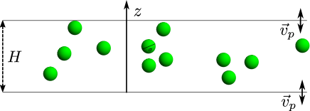
(b)

Figure 1: Schematic representation of the model for $d=3$ (1(a)), and for $d=2$ (1(b)).

with $v_{z}>0$. The symbol $\uparrow$ in the operator means that the particle collides with the top wall. As it was mentioned above, this simple model for a vibrating wall arises for a wall that moves sinusoidally with amplitude $A$, angular frequency $\omega$, in the limit $A\to 0$, $\omega\to\infty$ with $A\omega=v_{p}$. Note that both wall-particle collisions always inject energy into the system, while the tangential component of the velocity remains constant. Consequently, the linear momentum in the horizontal direction is a constant of motion. Let us remark that in the model the value of $v_{p}$ can be scaled. If the values of the walls are changed by a constant factor, i.e, $v_{p}\to Kv_{p}$ with $K>0$ and the velocities of the particles are modified by the same factor, the sequence of collisions is the same due to the linear character of the collision rule mgb19 . A schematic representation of the model for $d=3$ and $d=2$ is plotted in Figs. 1(a) and 1(b) respectively.

In the following, we will assume that the system is in the dilute limit and we will focus on obtaining a kinetic formulation of the model. We assume a closed description of the system in terms of the one-particle distribution function, $f({\bm{r}},{\bm{v}},t)$. Following standard arguments resibois1977classical ; dorfman2021contemporary ; mclennan1989introduction , the time evolution equation for the distribution function can be written as a sum of a free-streaming contribution and two parts corresponding to collisions: particle-particle and particle-wall collisions. In the low density limit, the particle-particle collisional term can be written as a functional of the one-particle distribution function by assuming Stosszahlansatz (molecular chaos), i.e., the velocities of colliding particles are uncorrelated and the evolution equation reads

$$\left(\frac{\partial}{\partial t}+\bm{v}\cdot\frac{\partial}{\partial\bm{r}}\right)f(\bm{r},\bm{v},t)=\mathcal{J}_{z}[f|f]+L_{W}f(\bm{r},\bm{v},t).$$ (5)

Here $\mathcal{J}_{z}[f|f]$ is the particle-particle collision term

$$\mathcal{J}_{z}[f|f]=\sigma^{d-1}\int\differential\bm{v}_{1}\int_{\Omega_{d}(H,z)}\differential\widehat{\bm{\sigma}}\,|\bm{g}\cdot\widehat{\bm{\sigma}}|\left[\Theta(\bm{g}\cdot\widehat{\bm{\sigma}})\alpha^{-2}b_{\sigma}^{-1}-\Theta(-\bm{g}\cdot\widehat{\bm{\sigma}})\right]f(\bm{r}_{1},\bm{v}_{1},t)f(\bm{r},\bm{v},t),$$ (6)

where we have introduced the Heaviside step function, $\Theta$, ${\bm{r}_{1}}\equiv\bm{r}+\sigma\widehat{\bm{\sigma}}$, and the inverse operator $b_{\widehat{\bm{\sigma}}}^{-1}$ that changes all velocities appearing to its right by the pre-collisional velocities

$$\bm{v}^{*} \equiv b_{\widehat{\bm{\sigma}}}^{-1}\bm{v}=\bm{v}+\frac{1+\alpha}{2\alpha}(\widehat{\bm{\sigma}}\cdot\bm{g})\widehat{\bm{\sigma}},$$ (7)

$$\bm{v}_{1}^{*} \equiv b_{\widehat{\bm{\sigma}}}^{-1}\bm{v}_{1}=\bm{v}_{1}-\frac{1+\alpha}{2\alpha}(\widehat{\bm{\sigma}}\cdot\bm{g})\widehat{\bm{\sigma}}.$$ (8)

The integral over the $d$-dimensional solid angle is taken over the allowed scattering angles, $\Omega_{d}(H,z)$, that depends on $H$ and $z$ due to the walls. For $d=3$, working in spherical coordinates being $\theta$ and $\phi$ the polar and azimuthal angles respectively, the domain $\Omega_{3}(H,z)$ can be parametrized as follows

$$\Omega_{3}(H,z)\equiv\left\{\begin{aligned} \hfil\displaystyle\begin{split}\{(\theta,\phi)|\;\theta\in(0,\pi/2+b_{1}(z)),\phi\in(0,2\pi)\},\;&\hbox{ if }z\in[\sigma/2,3\sigma/2],\\ \{(\theta,\phi)|\;\theta\in(0,\pi),\phi\in(0,2\pi)\},\;&\hbox{ if }z\in[3\sigma/2,H-3\sigma/2],\\ \{(\theta,\phi)|\;\theta\in(\pi/2-b_{2}(z),\pi),\phi\in(0,2\pi)\},\;&\hbox{ if }z\in[H-3\sigma/2,H-\sigma/2],\\ \end{split}\end{aligned}\right.$$ (9)

with

$$\begin{aligned} b_{1}(z)&=\sin^{-1}\left(\frac{z-\sigma/2}{\sigma}\right),\\ b_{2}(z)&=\sin^{-1}\left(\frac{H-\sigma/2-z}{\sigma}\right).\end{aligned}$$ (10)

In Fig. 2 (color online), a schematic diagram of the possible angles of collisions in a hard spheres system is plotted (purple region). It can be appreciated that, depending on $z$, three parts in the system can be distinguished: one “bulk” part where all collisions are possible and two “boundary” parts where the orientation of the collisions is restricted due to one of the walls. The “boundary” part is the region between the dot line and the closest wall (grey region). For $d=2$ the parametrization is similar. Defining $\theta$ as the angle between $\widehat{\bm{\sigma}}$ and ${\widehat{\bm{e}}}_{z}$, it is

$$\Omega_{2}(H,z)\equiv\left\{\begin{aligned} \hfil\displaystyle\begin{split}\theta\in(-\pi/2-b_{1}(z),\pi/2+b_{1}(z)),\;&\hbox{ if }z\in[\sigma/2,3\sigma/2],\\ \theta\in(-\pi,\pi),\;&\hbox{ if }z\in[3\sigma/2,H-3\sigma/2],\\ \theta\in(\pi/2-b_{2}(z),3\pi/2+b_{2}(z)),\;&\hbox{ if }z\in[H-3\sigma/2,H-\sigma/2],\\ \end{split}\end{aligned}\right.$$ (11)

where $b_{1}$ and $b_{2}$ are defined in Eq. (10). Finally, the wall term is written as in dorfman2021contemporary

$$L_{W}f({\bm{r}},{\bm{v}},t)=\left[\delta(z-H+\sigma/2)L_{\uparrow}+\delta(z-\sigma/2)L_{\downarrow}\right]f({\bm{r}},{\bm{v}},t),$$ (12)

with the operators given by

$$L_{\uparrow}f({\bm{r}},{\bm{v}},t) = \left[\Theta(-v_{z}-2v_{p})|2v_{p}+v_{z}|b_{\uparrow}-\Theta(v_{z})v_{z}\right]f(\bm{r},\bm{v},t),$$ (13)

$$L_{\downarrow}f({\bm{r}},{\bm{v}},t) = \left[\Theta(v_{z}-2v_{p})|2v_{p}-v_{z}|b_{\downarrow}-\Theta(-v_{z})|v_{z}|\right]f(\bm{r},\bm{v},t).$$ (14)

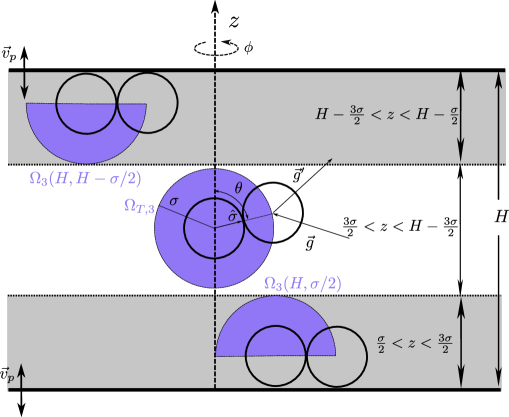
Figure 2: (Color online) Schematic diagram of the possible angles of collisions in a hard sphere system (purple region). It can be appreciated that, depending on $z$, three parts in the system can be distinguished: one “bulk” part where all collisions are possible and two “boundary” parts where the orientation of the collisions is restricted due to one of the walls. The “boundary” part is the region between the dot line and the closest wall (grey region).

Note that in the particle-particle collisional contribution defined in Eq. (6), the particles are considered to be at two different points, $\bm{r}$ and $\bm{r}_{1}$. This is in contrast with the “traditional” Boltzmann equation and it is necessary in order to obtain a consistent equation.

In the following, we will assume that the system is thin and dilute enough so that the dependence of $f(\bm{r},\bm{v},t)$ on $z$ can be neglected. Under this approximation the distribution function can be substituted by its average along the $z$-coordinate, i.e.

$$f(\bm{r},\bm{v},t)\approx f(\bm{r}_{\parallel},\bm{v},t)\equiv\frac{1}{(H-\sigma)}\int_{\sigma/2}^{H-\sigma/2}\differential{z}\leavevmode\nobreak\ f(\bm{r},\bm{v},t),$$ (15)

with $\bm{r}\equiv\bm{r}_{\parallel}+z\widehat{\bm{e}}_{z}$. Therefore, integrating Eq. (5) over $z$, and taking into account the different domains of solid angles defined in Eqs. (9), gives rise to a closed evolution equation for $f(\bm{r}_{\parallel},\bm{v},t)$ given by

$$\left(\frac{\partial}{\partial t}+\bm{v}_{\parallel}\cdot\frac{\partial}{\partial\bm{r}_{\parallel}}\right)f(\bm{r}_{\parallel},\bm{v},t)=\frac{1}{(H-\sigma)}\int_{\sigma/2}^{H-\sigma/2}dz\mathcal{J}_{z}[f|f]+\frac{1}{(H-\sigma)}(L_{\uparrow}+L_{\downarrow})f(\bm{r}_{\parallel},\bm{v},t).$$ (16)

Interestingly, the particle-particle collision term verifies

$$\frac{1}{(H-\sigma)}\int_{\sigma/2}^{H-\sigma/2}dz\mathcal{J}_{z}[f|f]=\frac{\varepsilon-1}{\varepsilon}\mathcal{J}[f|f]+\frac{1}{\varepsilon}\mathcal{\widetilde{J}}[f|f],$$ (17)

where we have defined

$$\mathcal{J}[f|f]=\sigma^{d-1}\int\differential\bm{v}_{1}\int_{\Omega_{T,d}}\differential\widehat{\bm{\sigma}}\Theta(-\bm{g}\cdot\widehat{\bm{\sigma}})|\bm{g}\cdot\widehat{\bm{\sigma}}|(\alpha^{-2}b_{\sigma}^{-1}-1)f(\bm{r}_{\parallel},\bm{v}_{1},t)f(\bm{r}_{\parallel},\bm{v},t),$$ (18)

and

$$\mathcal{\widetilde{J}}[f|f]=\sigma^{d-2}\int^{3\sigma/2}_{\sigma/2}\differential z\int\differential\bm{v}_{1}\int_{\Omega_{d}(2\sigma,z)}\differential\widehat{\bm{\sigma}}\,\Theta(-\bm{g}\cdot\widehat{\bm{\sigma}})|\bm{g}\cdot\widehat{\bm{\sigma}}|(\alpha^{-2}b_{\sigma}^{-1}-1)f(\bm{r}_{\parallel},\bm{v}_{1},t)f(\bm{r}_{\parallel},\bm{v},t),$$ (19)

with $\Omega_{T,d}$ being the total solid angle in $d$ dimensions, and $\varepsilon\equiv(H-\sigma)/\sigma$. Hence, it splits in two terms, $\frac{\varepsilon-1}{\varepsilon}\mathcal{J}$ and $\varepsilon^{-1}\mathcal{\widetilde{J}}$. The first term corresponds with the collisional contribution of a system of height $(H-2\sigma)$ without restrictions in the angular integration and the second term is the collisional term of a system of height $2\sigma$ taking into account all the geometrical constraints. For $H\sim 2\sigma$ ($\varepsilon\sim 1$), $\frac{\varepsilon-1}{\varepsilon}\mathcal{J}$ can be neglected compared to $\varepsilon^{-1}\mathcal{\widetilde{J}}$. In this case, for $d=3$, Eq. (16) reduces to the one obtained in mgb19 for an ultra-confined system with $H=2\sigma$. In the opposite limit, i.e. $H\gg\sigma$($\varepsilon\gg 1$), the $\frac{\varepsilon-1}{\varepsilon}\mathcal{J}$ terms dominates with respect to $\varepsilon^{-1}\mathcal{\widetilde{J}}$ and the dynamics is the one of a “bulk” system of height $(H-2\sigma)\sim H$. This is consistent with the fact that, in this limit, the geometrical restrictions should not be relevant. Let us remark that, in order to have this decomposition, the homogeneous in $z$ approximation given by Eq. (15) is essential. In the same lines, the limit $H\gg\sigma$ is only meaningful if the above mentioned approximation is fulfilled. Henceforth, we will consider Eq. (16) as the dynamical equation of the system.

III Evolution equations for the horizontal and vertical temperatures

In the previous section, we have obtained a closed kinetic equation for a confined system averaged over $z$ direction in the low density regime, Eq. (16), that admits a spatially homogeneous solution of the form $f(\bm{v},t)$, i.e. a distribution independent of the horizontal spatial variables. In this section, the evolution equations for the partial temperatures associated to the horizontal and vertical degrees of freedom, $T$ and $T_{z}$, are studied for this spatially homogeneous state. The partial temperatures $T$ and $T_{z}$ are defined as usual in kinetic theory

$$(d-1)\frac{n}{2}T(t)=\int\differential\bm{v}\,\frac{m}{2}v_{\parallel}^{2}f(\bm{v},t),$$ (20)

$$\frac{n}{2}T_{z}(t)=\int\differential\bm{v}\,\frac{m}{2}v_{z}^{2}f(\bm{v},t),$$ (21)

with $v_{\parallel}^{2}\equiv\sum_{i=1}^{d-1}v_{i}^{2}$ is the sum over all the horizontal coordinates and $n$ is the number density defined by $n\equiv N/(H-\sigma)L^{d-1}$. We assume that there is no macroscopic velocity, i.e., $\int\differential{\bm{v}}\,\bm{v}f({\bm{v}},t)=\bm{0}$. This assumption holds for all symmetric distribution functions in the variable ${\bm{v}}$, i.e., $f({\bm{v}})=f({-\bm{v}})$. To obtain the evolution equations for the temperatures, we take velocity moments in the Boltzmann-like equation given by Eq. (16). First, the evolution equation of the horizontal temperature is obtained by multiplying $\frac{m}{2}v_{\parallel}^{2}$ in Eq. (16) and integrating over all velocities. This leads to

$$(d-1)\frac{n}{2}\derivative{T}{t}=\frac{m}{2(H-\sigma)}\int_{\sigma/2}^{H-\sigma/2}dz\int\differential{\bm{v}}\,v_{\parallel}^{2}\,\mathcal{J}_{z}[f|f],$$ (22)

where the wall collision term trivially vanishes because there is not energy injection in the horizontal direction. We proceed in the same way to deduce the equation for vertical temperature. It can be written as

$$\frac{n}{2}\derivative{T_{z}}{t}=\frac{m}{2(H-\sigma)}\int_{\sigma/2}^{H-\sigma/2}dz\int\differential{\bm{v}}\,v_{z}^{2}\,\mathcal{J}_{z}[f|f]+\frac{m}{2(H-\sigma)}\int\differential{\bm{v}}\,v_{z}^{2}(L_{\uparrow}+L_{\downarrow})f(\bm{v},t).$$ (23)

In this case, the wall terms appear since both walls inject energy in the vertical direction. To obtain closed equations for the partial temperatures, it is assumed that the velocity distribution is an asymmetric maxwellian with two different temperatures, associated to the horizontal and vertical directions

$$f(\bm{v},t)=\frac{n}{\pi^{\frac{d}{2}}w^{d-1}(t)w_{z}(t)}\,{\rm exp}\bigg{[}-\frac{v^{2}_{\parallel}}{w^{2}(t)}-\frac{v^{2}_{z}}{w^{2}_{z}(t)}\bigg{]},$$ (24)

where we have introduced the thermal velocities

$$\frac{m}{2}w^{2}(t)\equiv T(t),$$ (25)

$$\frac{m}{2}w^{2}_{z}(t)\equiv T_{z}(t).$$ (26)

In the ansatz given by Eq. (24) correlations between the horizontal and vertical degrees of freedom are neglected. This is validated in the next sections by comparing the theoretical results with MD simulations for $d=2$ and $d=3$.

In order to solve the integrals given in Eqs. (22) and (23), the following fundamental property of the particle-particle collision term is used

$$\frac{1}{(H-\sigma)}\int_{\sigma/2}^{H-\sigma/2}\differential z\int\differential\bm{v}\,\psi(\bm{v})\mathcal{J}_{z}[f|f]= \frac{\sigma^{d-1}}{2(H-\sigma)}\int_{\sigma/2}^{H-\sigma/2}\differential z\int\differential\bm{v}_{1}\int\differential\bm{v}f(\bm{v}_{1},t)f(\bm{v},t)$$

$$\times\int_{\Omega_{d}(H,z)}\differential\widehat{\bm{\sigma}}\;\absolutevalue{\bm{g}\cdot\widehat{\bm{\sigma}}}\Theta(\bm{g}\cdot\widehat{\bm{\sigma}})(b_{{\widehat{\bm{\sigma}}}}-1)\{\psi(\bm{v}_{1})+\psi(\bm{v})\},$$ (27)

where $\psi(\bm{v})$ is an arbitrary velocity function. In Appendix A the corresponding property for the particle-wall collision operators is derived, obtaining

$$\int\differential\bm{v}\,\psi(\bm{v})L_{\uparrow}f(\bm{v},t)= \int\differential\bm{v}\;f(\bm{v},t)\absolutevalue{v_{z}}\Theta(v_{z})(b_{\uparrow}-1)\psi(\bm{v}),$$ (28)

$$\int\differential\bm{v}\,\psi(\bm{v})L_{\downarrow}f(\bm{v},t)= \int\differential\bm{v}\;f(\bm{v},t)\absolutevalue{v_{z}}\Theta(-v_{z})(b_{\downarrow}-1)\psi(\bm{v}).$$ (29)

Note that the left-hand side of Eqs. (III)-(29) corresponds to the rate of change of $\langle\psi\rangle\equiv\int\differential v\,\psi f(\bm{v},t)$ due to collisions. In our case, we study the variation rate of temperature in each space coordinate, i.e., how the mean values of $v_{\parallel}^{2}$ and $v_{z}^{2}$ change. Using the relations given in (III)-(29), the collisional integrals can be written as (see Appendix B)

$$\begin{aligned} \frac{m}{2(H-\sigma)}\int_{\sigma/2}^{H-\sigma/2}dz\int\differential{\bm{v}}\,v_{\parallel}^{2}\,\mathcal{J}_{z}[f|f]=&\frac{mn^{2}\sigma^{d-1}(1+\alpha)\Omega_{T,d-1}\;w^{3}}{\sqrt{2\pi}\varepsilon}\int_{0}^{1}\differential y\;\big{(}1+\beta y^{2}\big{)}^{1/2}(1-y^{2})^{\frac{(d-1)}{2}}\\ &\times\left[\frac{(1+\alpha)}{2}\big{(}1+\beta y^{2}\big{)}-1\right][(\varepsilon-1)+(1-y)],\\ \end{aligned}$$ (30)

$$\begin{aligned} \frac{m}{2(H-\sigma)}\int_{\sigma/2}^{H-\sigma/2}dz\int\differential{\bm{v}}\,v_{z}^{2}\,\mathcal{J}_{z}[f|f]=&\frac{mn^{2}\sigma^{d-1}(1+\alpha)\Omega_{T,d-1}\;w^{3}}{\sqrt{2\pi}\varepsilon}\int_{0}^{1}\differential y\;\big{(}1+\beta y^{2}\big{)}^{1/2}(1-y^{2})^{\frac{(d-3)}{2}}\\ &\times y^{2}\left[\frac{(1+\alpha)}{2}\big{(}1+\beta y^{2}\big{)}-(1+\beta)\right][(\varepsilon-1)+(1-y)],\end{aligned}$$ (31)

where $\beta\equiv\frac{T_{z}}{T}-1$. Note that both integrals split into two terms: one term proportional to $(\varepsilon-1)$, plus other term that corresponds to the results of Ref. mgb19 for $H=2\sigma$ ($\varepsilon=1$), in agreement with the property given by Eq. (17). On the other hand, the integral corresponding to collision with walls is

$$\frac{m}{2(H-\sigma)}\int\differential\bm{v}v_{z}^{2}(L_{\uparrow}+L_{\downarrow})f(\bm{v},t)=2\frac{nv_{p}T_{z}}{(H-\sigma)}.$$ (32)

Note that Eq. (32) is twice the injection of energy term obtained in a system with a vibrated monolayer when only one wall is moving mgb19 . This equivalence is consistent because the double of energy is injected by the walls.

The integrals (30) and (31) can be solved exactly, but the expressions are quite complex to handle with. To get a simpler theoretical analysis, we perform a first order expansion considering $\beta\ll 1$, i.e., the horizontal and vertical temperatures are close. In this case, the equations are

$$\derivative{T}{t}= \frac{n\sigma^{d-1}(1+\alpha)\Omega_{T,d}\;w}{\sqrt{2\pi}d\left(2+d\right)\varepsilon}T\left\{(\varepsilon-1)\bigg{[}-(2+d)(1-\alpha)+\frac{(1+3\alpha)}{2}\beta\bigg{]}\right.$$ (33)

$$\left.-g(d)(1-\alpha)+\frac{(1+3\alpha)h(d)}{2}\beta\right\},$$

$$\derivative{T_{z}}{t}= -\frac{n\sigma^{d-1}(1+\alpha)\Omega_{T,d}\;w}{\sqrt{2\pi}d\left(2+d\right)\varepsilon}T\left\{(\varepsilon-1)\bigg{[}(2+d)(1-\alpha)+\frac{(5+4d-9\alpha)}{2}\beta\bigg{]}\right.$$ (34)

$$\left.g_{z}(d)(1-\alpha)+\frac{4g_{z}(d)-(1+3\alpha)h_{z}(d)}{2}\beta\right\}+\frac{4v_{p}T_{z}}{\sigma\varepsilon},$$

with

$$g(d) \equiv (2+d)-\frac{4(3+d)\;\Gamma\left(2+\frac{d}{2}\right)}{\left[(2+d)^{2}-1\right]\sqrt{\pi}\;\Gamma\left(\frac{d+1}{2}\right)},$$ (35)

$$h(d) \equiv 1-\frac{8\;\Gamma\left(2+\frac{d}{2}\right)}{\left[(2+d)^{2}-1\right]\sqrt{\pi}\;\Gamma\left(\frac{d+1}{2}\right)},$$ (36)

$$g_{z}(d) \equiv (2+d)-\frac{16\;\Gamma\left(2+\frac{d}{2}\right)}{(d^{2}-1)\sqrt{\pi}\;\Gamma\left(\frac{d-1}{2}\right)},$$ (37)

$$h_{z}(d) \equiv 6-\frac{64\;\Gamma\left(2+\frac{d}{2}\right)}{(3+d)(d^{2}-1)\sqrt{\pi}\;\Gamma\left(\frac{d-1}{2}\right)},$$ (38)

where $\;\Gamma\left(z\right)\equiv\int_{0}^{\infty}\differential t\;t^{z-1}e^{-t}$ is the Gamma function. Let us briefly analyze Eqs. (33) and (34). First, note that, in agreement with Eq. (17), two separated terms are obtained in the particle-particle collisional contribution of both equations: One of them is multiplied by a factor $(\varepsilon-1)$ becoming dominant for $H\gg\sigma$, while the other dominates for $H=2\sigma$, where the first term vanishes. If the zeroth order in $\beta$ is considered and $v_{p}=0$ is taken, in the limit of $H\gg\sigma$, the temperature evolution equation of a freely evolving granular gas is obtained in the gaussian approximation van1998velocity . We also remark that the Eqs. (33) and (34) are obtained assuming $\beta\ll 1$, so that the equations are only valid if the horizontal and vertical temperatures are of the same order of magnitude, i.e., $T\approx T_{z}$. The $\beta$ terms in Eqs. (33) and (34) describe the energy transfer between the vertical and horizontal degrees of freedom due to particle collisions, while the last term of Eq. (34) describes the energy injection term due to the walls. Thus, the dynamics can be summarized as follows: wall-particle collisions inject energy in the vertical direction, particle-particle collisions transfer energy from the vertical to the horizontal degrees of freedom, while energy is dissipated through inelastic collisions. The main difference with the corresponding equations in the ultra-confined system mgb19 , is that energy is also dissipated in the vertical degree of freedom.

From Eqs. (33) and (34) the stationary partial temperatures, $T_{s}$ and $T_{z,s}$, can be obtained. In particular, from Eq. (33), the quotient between the stationary temperatures, $\beta_{s}\equiv\frac{T_{z,s}}{T_{s}}-1$, is easily calculated, obtaining

$$\beta_{s}=K(d,\varepsilon)\frac{1-\alpha}{1+3\alpha},$$ (39)

where

$$K(d,\varepsilon)=2\frac{(d+2)(\varepsilon-1)+g(d)}{\varepsilon-1+h(d)},$$ (40)

is a geometric factor that depends on the height of the system and the spatial dimensionality. Hence, $\beta_{s}$ depends on the inelasticity, height and $d$, but it is density independent. $\beta_{s}$ is always positive in the range $0<\alpha<1$, so that $T_{z,s}$ is always larger than $T_{s}$, consistent with the fact that energy is injected in the vertical direction and then transferred to the horizontal one. Moreover, for a given height, $\beta_{s}$ decreases monotonically with the inelasticity, vanishing in the elastic limit, in accordance with equipartition. Note that this property is not obvious, as the elastic limit could be singular (equipartition obviously holds in the elastic case with $v_{p}=0$). At constant inelasticity, $\beta_{s}$ decays monotonically with the height. Intuitively, this was expected to happen because, the thinner the system is, the more anisotropic is. In the $\varepsilon\gg 1$ limit, the following simple asymptotic expression is obtained

$$\beta_{s}\sim\beta_{s}^{(\infty)}\equiv\frac{2(d+2)(1-\alpha)}{1+3\alpha},\quad\text{for}\quad\varepsilon\gg 1.$$ (41)

The expression for $\beta_{s}$ given by Eq. (39) is only valid in the small $\beta$ case. Nevertheless, from Eq. (30) a closed equation for $\beta_{s}$ can be obtained that is valid, in principle, for arbitrary $\beta$ (of course, its validity depends on the validity of the maxwellian ansatz) and that has been solved numerically. In Fig. 3 (color online) the approximate expression for $\beta_{s}$ given by Eq. (39) (solid lines) and the one coming from Eq. (30) (dashed lines) are plotted for $d=3$ as a function of the inelasticity. We have considered two values of the height, $H=2\sigma$ (black) and $H=29\sigma$ (blue). The quasi-elastic region is enlarged in the inset. It can be seen that the approximate expression for $\beta_{s}$ and the one coming from Eq. (30) are very similar from the elastic limit till $\alpha\sim 0.8$ (where $\beta\sim 1$). Similar results are obtained for $d=2$. In Fig. 4 (color online) the approximate expression for $\beta_{s}$ given by Eq. (39) (solid lines) and the one coming from Eq. (30) (dashed lines) are plotted for $d=3$ as a function of the dimensionless height, $\epsilon$. We have considered two values of the inelasticity, $\alpha=0.6$ (black) and $\alpha=0.9$ (blue). For $\alpha=0.9$ both curves are very similar except close to $\varepsilon=1$ ($H=2\sigma$) where $\beta_{s}$ is not sufficiently small for the approximation to be valid. For $\alpha=0.6$, the inelasticity induces a stronger anisotropy bgm19 in such a way that the approximation is no longer accurate, independently of the height of the system. For both inelasticities it is seen that the bulk expression accurately describes a wide range of heights, for values of $\varepsilon$ larger than approximately $2$.

Figure 3: (Color online) Theoretical expressions for $\beta_{s}$ given by Eq. (39) (solid lines) and by the numerical solution coming from (30) (dashed lines) for $d=3$ as a function of the inelasticity. Two values of the height are considered: $H=2\sigma$ (black) and $H=29\sigma$ (blue). The quasi-elastic region is enlarged in the inset.

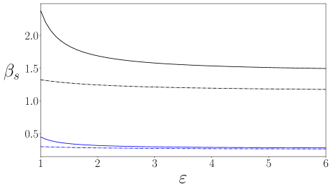
Figure 4: (Color online) Theoretical expressions for $\beta_{s}$ given by Eq. (39) (solid lines) and by the numerical solution coming from (30) (dashed lines) for $d=3$ as a function of the dimensionless height, $\epsilon$. Two values of the inelasticity are considered: $\alpha=0.6$ (black) and $\alpha=0.9$ (blue).

By Inserting $\beta_{s}$ giving by Eq. (39) into Eq. (34), the stationary horizontal temperature can be calculated, obtaining

$$\left[\frac{T_{s}}{mv_{p}^{2}}\right]^{1/2}=\frac{4\sqrt{\pi}d(d+2)(1+\beta_{s})}{(1+\alpha)\Omega_{T,d}\left[C(d,\alpha,\varepsilon)+D(d,\alpha,\varepsilon)(\varepsilon-1)]\right\}n\sigma^{d}},$$ (42)

where the following functions

$$C(d,\alpha,\varepsilon) = (1-\alpha)g_{z}(d)+[4g_{z}(d)-(1+3\alpha)h_{z}(d)]\frac{\beta_{s}}{2},$$ (43)

$$D(d,\alpha,\varepsilon) = (1-\alpha)(d+2)+(5+4d-9\alpha)\frac{\beta_{s}}{2},$$ (44)

have been introduced. Independently of the complex behavior of $T_{s}$ as a function of the inelasticity and the height, that will be discussed later, the density dependence is very simple, $T_{s}\sim(n\sigma^{d})^{-2}$. This dependence comes from the fact that the number of wall-particle collisions grows with $n\sigma^{d}$, while the number of particle-particle collisions grows with $(n\sigma^{d})^{2}$. Then, the more dilute the system is, the more energy is injected. Moreover, the stationary pressure defined as $p(n)\equiv nT_{s}(n)$ goes as $(n\sigma^{d})^{-1}$ and the steady state compressibility, $\kappa\equiv\derivative{p}{n}$, is negative. This macroscopic property is similar to the one observed in vibrated ultra-confined Q2D systems mgb19b , in which the negative compressibility is the essential ingredient that triggers the instability. We will further discuss this point in the last section. Note that the temperature diverges in the elastic limit, $\alpha\to 1$, because there is no energy loss mechanisms. For $\varepsilon\gg 1$, Eq. (42) is simplified, obtaining

$$\left[\frac{T_{s}}{mv_{p}^{2}}\right]^{1/2}\sim\frac{4\sqrt{\pi}d(d+2)(1+\beta_{s}^{(\infty)})}{(1+\alpha)\Omega_{T,d}D(d,\alpha,\infty)\varepsilon n\sigma^{d}},\quad\text{for}\quad\varepsilon\gg 1,$$ (45)

where $D(d,\alpha,\infty)\equiv\lim_{\varepsilon\to\infty}D(d,\alpha,\varepsilon)=(1-\alpha)(d+2)+(5+4d-9\alpha)\frac{\beta_{s}^{(\infty)}}{2}$. Note that, in this asymptotic regime, the dependence on the size of the system is very simple, i.e. $T_{s}\propto\varepsilon^{-2}$. On the other hand, we have also obtained $T_{s}$ using the exact solutions given in Eqs. (29) and (30). However, no difference between both expressions are appreciated in the relevant range of parameters.

The objective now it to study the stability of the stationary solution in the context of Eqs. (33) and (34), i.e., it is assumed that there are not gradients and that the dynamics is given in terms of the above mentioned equations. In order to perform the analysis, it is convenient to introduce the following dimensionless time scale

$$s(t)=\frac{n\sigma^{d-1}(1+\alpha)\Omega_{T,d}\ }{\sqrt{2\pi}d\left(2+d\right)\varepsilon}\int^{t}_{0}d\tau w(\tau),$$ (46)

that is proportional to the collisions per particle in $(0,t)$. We will consider small deviations around the stationary temperatures, so that Eqs. (33) and (34) can be linearized. The deviations $\delta T\equiv T-T_{s}$ and $\delta T_{z}\equiv T_{z}-T_{z,s}$ obey the following system of ordinary differential equations that can be expressed in matrix form as follows

$$\frac{d}{ds}\begin{pmatrix}\delta T\\ \delta T_{z}\end{pmatrix}=M\begin{pmatrix}\delta T\\ \delta T_{z}\end{pmatrix},$$ (47)

where $M$ is the matrix

$$M=-\begin{pmatrix}(1-\alpha)A+\frac{B}{2}&\;-\frac{B}{2}\\ \frac{3(1-\alpha)}{2}A_{z}+\frac{(\beta_{s}-2)}{2}\frac{B_{z}}{2}&\frac{1}{1+\beta_{s}}\Big{[}\frac{B_{z}}{2}-(1-\alpha)A_{z}\Big{]}\end{pmatrix},$$ (48)

with

$$A\equiv (2+d)(\varepsilon-1)+g(d),$$ (49)

$$B\equiv [\varepsilon-1+h(d)](1+3\alpha),$$ (50)

$$A_{z}\equiv (2+d)(\varepsilon-1)+g_{z}(d),$$ (51)

$$B_{z}\equiv (5+4d-9\alpha)(\varepsilon-1)+4g_{z}(d)-(1+3\alpha)h_{z}(d).$$ (52)

The eigenvalues of the matrix $M$ have been calculated numerically obtaining that its real part is always negative, so that the stationary state is linearly stable. For mild inelasticities, two different real eigenvalues are obtained, $\lambda_{2}<\lambda_{1}<0$, so that, for long times, the dynamics is dominated by the slowest eigenvalue, $\lambda_{1}$, that defines the hydrodynamic time scale. Interestingly, for strong inelasticities, the eigenvalues turn complex, and the stationary state is reached oscillating. This happens for $\alpha\sim 0.7$, independently of the other parameters. The origin and the possible implications in the hydrodynamic description of the system of this transition will be studied in detail elsewhere mgmTBP .

IV Simulation results

By using the Event-Driven algorithm allen , we have performed MD simulations of an ensemble of inelastic hard spheres or disks confined between two sawtooth walls perpendicular to the $z$-direction. The vibrating walls are separated a distance $H$ and periodic boundary conditions are applied in the horizontal direction. We have taken $m$ and $\sigma$ as the unit of mass and length, respectively. To generate the initial condition, the particles are placed inside the system at random, with a two-temperature gaussian velocity distribution, being the initial horizontal temperature, $T(0)$, the unit of energy. The initial vertical temperature has been chosen between $0.1T(0)$ and $10T(0)$, depending on the simulation. The velocity of both walls is $v_{p}=0.001\left[\frac{T(0)}{m}\right]^{1/2}$. For $d=3$, we have taken $N=512$ and $n\sigma^{3}=0.02$ and for $d=2$, $N=300$ and $n\sigma^{2}=0.02$, so that the system can be considered to be dilute and the kinetic theory description of the previous section is expected to be valid. The results have been averaged over $10$ realizations. Let us remark that the simulations in our confined system run much more slowly than in the non-confined system due to the huge number of collisions with the walls. In any case, the considered number of particles is large enough for the Boltzmann equation to be valid mgb19 and the number of realizations suffices to have a good statistic to validate the theory. For different values of the height and the inelasticity, we have checked that the system remains in a spatially homogeneous state for all the time evolution. In Fig. 5 a typical snapshot of the system (observed from above) is shown. No density gradients are appreciated. The values of the parameters are the ones for $d=3$ with $H=8\sigma$ and $\alpha=0.9$.

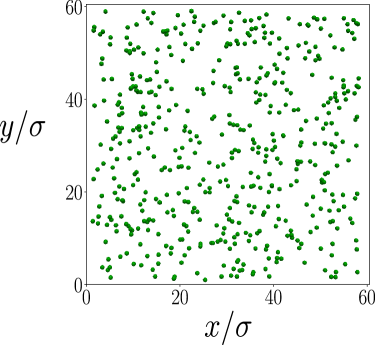
Figure 5: Snapshot of a typical configuration of a hard spheres system (observed from above). The values of the parameters are the ones for $d=3$ with $H=8\sigma$ and $\alpha=0.9$.

We have performed a more quantitative analysis by measuring the hydrodynamic fields in the horizontal and vertical directions. For all the values of the parameters that are considered in this section, it was found that the system is spatially homogeneous with a high degree of accuracy. For example, the dimensionless vertical averaged density, $n_{z}(z)\sigma^{3}\equiv\frac{1}{L^{2}}\int dx\int dy\,n(\mathbf{r})\sigma^{3}$, is plotted in Fig. 6 as a function of $z/\sigma$ for a hard spheres system with $H=8\sigma$ and $\alpha=0.9$. The error bars are obtained from the average over the $10$ realizations. The density fluctuates around its mean value, $n\sigma^{3}=0.02$, showing that the system is homogeneous in the vertical direction with a high degree of accuracy. Similar results are obtained for the other values of the parameters considered in this section.

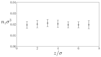
Figure 6: Dimensionless vertical averaged density, $n_{z}(z)\sigma^{3}$, as a function of $z/\sigma$ for a hard spheres system with $H=8\sigma$ and $\alpha=0.9$. The error bars are obtained from the average over the $10$ realizations.

For strong inelasticities, some simulations showed the development of clusters of particles. Of course, these simulations were discarded. We have also measured the marginals one-particle distribution functions. In Fig. 7 (color online), the simulation results for the logarithm of the marginals velocity distribution functions once the stationary state is reached, $f_{s,x}(v_{x})\equiv\int dv_{y}\int dv_{z}f_{s}(\mathbf{v})$ (red circles) and $f_{s,z}(v_{z})\equiv\int dv_{x}\int dv_{y}f_{s}(\mathbf{v})$ (green squares), are plotted for $H=5\sigma$ and $\alpha=0.65$. The (red) dashed line and the (green) solid line are the corresponding quadratic interpolations that fit accurately the simulation results. Similar results are obtained for the transient to the stationary state and for other values of the parameters, showing the accuracy of the ansatz given by Eq. (24).

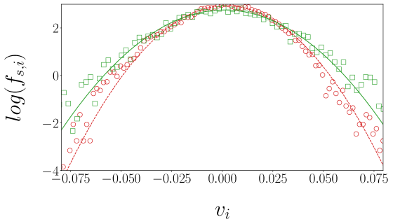
Figure 7: Simulation results for the logarithm of the stationary marginals velocity distribution functions, $f_{s,x}$ (red circles) and $f_{s,z}$ (green squares), as functions of $v_{x}$ and $v_{z}$, respectively, for $H=5\sigma$ and $\alpha=0.65$. The (red) dashed line and the (green) solid line are the corresponding quadratic interpolations.

In Fig. 8(a), the stationary quotient of temperatures of a system of hard spheres is plotted as a function of $\alpha$ for $H=5\sigma$. The circles are the simulation results, the solid line is the linear approximation of $\beta_{s}$ given by Eq. (39) and the dashed line is the numerical theoretical prediction coming from Eq. (30). The error bars are obtained from the average over the $10$ realizations. The quasi-elastic region is enlarged in the inset. It is seen that $\beta_{s}$ decays monotonically with the inelasticity vanishing in the elastic limit, where equipartition holds. A very good agreement is found between the simulation results and the theoretical prediction coming from Eq. (30) in the whole range of inelasticities. Stronger inelasticities are not consider because the homogeneous state becomes unstable. The agreement with Eq. (39) is also good for mild inelasticities where $\beta_{s}$ is still small, consistently with the linear approximation. The same is plotted in Fig. 8(b), but for $H=29\sigma$. As for $H=5\sigma$, a very good agreement is found between the simulation results and the theoretical predictions. Note that, for a given $\alpha$, the values of $\beta_{s}$ for $H=5\sigma$ and for $H=29\sigma$ are very close. This is in contrast with the ultra-confined system where $\beta_{s}$ strongly depends on $H$ mgb19 .

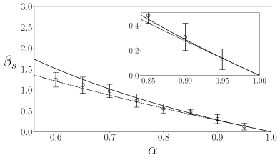
(a)

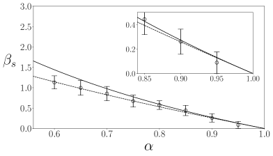
(b)

Figure 8: $\beta_{s}$ of a hard spheres system as a function of $\alpha$ for $H=5\sigma$ (a) and $H=29\sigma$ (b). The circles are the simulation results, the solid line is the linear approximation of $\beta_{s}$ given by Eq. (39) and the dashed line is the numerical theoretical prediction coming from Eq. (30). The error bars are obtained from the average over the $10$ realizations. The quasi-elastic region is enlarged in the inset.

For hard disks, a very similar behavior is obtained, but for a more restricted range of inelasticities, because clusters of particles are developed for larger values of $\alpha$. In Fig. 9 (color online), $\beta_{s}$ is plotted as a function of $\alpha$ for $H=10\sigma$ and $H=29\sigma$. The (black) circles are the simulation results for $H=10\sigma$ and the (red) squares for $H=29\sigma$. The error bars are obtained from the average over the $10$ realizations. The (black) solid line is the theoretical prediction for $H=10\sigma$ and the (red) dashed line for $H=29\sigma$, both given by Eq. (39). The inset shows the quasi-elastic region. In this case, it is not necessary to go beyond the linear approximation as the range of inelasticities is restricted to mild inelasticities. In fact, for $H=10\sigma$, clusters are developed for $\alpha<0.975$. In Fig. 10, the dependence of $\beta_{s}$ with the dimensionless height, $\varepsilon$, is studied in a hard sphere system for two different values of the inelasticity. The (black) squares are the simulation results for $\alpha=0.6$ and the (blue) circles for $\alpha=0.9$. The error bars are obtained from the average over the $10$ realizations. The (black) point line is the theoretical prediction for $\alpha=0.6$ and the (blue) solid line for $\alpha=0.9$, both given by the numerical theoretical prediction coming from Eq. (30). A good agreement between the theoretical prediction and the simulation results is obtained. For $\varepsilon\sim 1$, it is appreciated that the small deviation of $\beta_{s}$ with respect to the “bulk” contribution is captured by the theory. Similar results are obtained for hard disks.

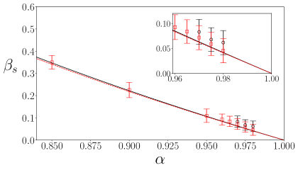
Figure 9: (Color online) $\beta_{s}$ of a hard disks system as a function of $\alpha$ for $H=10\sigma$ and $H=29\sigma$. The (black) circles are the simulation results for $H=10\sigma$ and the (red) squares for $H=29\sigma$. The error bars are obtained from the average over the $10$ realizations. The (black) solid line is the theoretical prediction for $H=10\sigma$ and the (red) dashed line for $H=29\sigma$, both given by Eq. (39). The inset shows the quasi-elastic region.

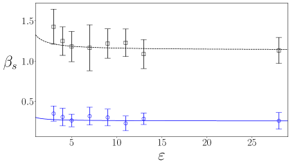
Figure 10: (Color online) $\beta_{s}$ of a hard sphere system as a function of the dimensionless height, $\varepsilon$, for $\alpha=0.6$ and $\alpha=0.9$. The (black) squares are the simulation results for $\alpha=0.6$ and the (blue) circles for $\alpha=0.9$. The error bars are obtained from the average over the $10$ realizations. The (black) point line is the theoretical prediction for $\alpha=0.6$ and the (blue) solid line for $\alpha=0.9$, both given by the numerical theoretical prediction coming from Eq. (30).

The dimensionless horizontal stationary temperature, $\frac{T_{s}}{mv_{p}^{2}}$, is plotted in Figs. 11(a) and 11(b) (color online) for hard spheres and disks respectively as a function of the inelasticity for different values of the height. The (red) circles, (black) squares and (blue) triangles are the simulation results for $H=8\sigma$, $H=10\sigma$ and $H=14\sigma$, respectively. The error bars are obtained from the average over the $10$ realizations. The (red) solid line, (black) dashed line and (blue) solid-dashed line are the corresponding theoretical predictions given by Eq. (42). The numerical solution valid beyond the linear regime in $\beta_{s}$ is not plotted because no difference between both curves can be appreciated. For a given height, the horizontal temperature increases with $\alpha$ because there is less dissipation of energy in particle-particle collisions. For a given inelasticity, the horizontal temperature decreases with the height as there are less particle-wall collisions. The agreement between the simulation results and the theoretical prediction is excellent for the whole range of considered parameters. In Fig. 12 (color online), the dimensionless horizontal stationary temperature, $\frac{T_{s}}{mv_{p}^{2}}$, is plotted as a function of $\varepsilon$ in logarithmic scale. The (blue) circles and the (black) squares are hard spheres simulation results for $\alpha=0.9$ and $\alpha=0.6$ respectively. The (green) triangles are hard disks simulation results for $\alpha=0.98$. The error bars are not plotted because they can not be seen in the scale of the figure. The (blue) solid line, (black) dashed line and (green) solid-dashed line are the corresponding theoretical prediction given by Eq. (42). The (red) point line is a straight line with slope $-2$ (showing the “bulk” prediction) that is plotted only for reference. It is seen that the agreement between the theory and the simulations is very good and that the corrections with respect to the bulk prediction are even smaller than for $\beta_{s}$ in the whole range of heights. No more values of the inelasticity are considered for hard disks because, for smaller values of the inelasticity, the system is unstable for most of the values of $\varepsilon$.

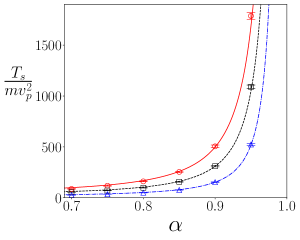
(a)

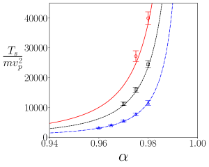
(b)

Figure 11: (Color online) Dimensionless horizontal stationary temperature, $\frac{T_{s}}{mv_{p}^{2}}$, for hard spheres (a) and disks (b) as a function of the inelasticity for different values of the height. The (red) circles, (black) squares and (blue) triangles are the simulation results for $H=8\sigma$, $H=10\sigma$ and $H=14\sigma$, respectively. The error bars are obtained from the average over the $10$ realizations. The (red) solid line, (black) dashed line and (blue) solid-dashed line are the corresponding theoretical predictions given by Eq. (42).

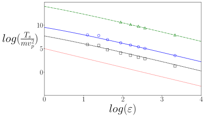
Figure 12: (Color online) Dimensionless horizontal stationary temperature, $\frac{T_{s}}{mv_{p}^{2}}$, as a function of $\varepsilon$ in logarithmic scale. The (blue) circles and the (black) squares are hard spheres simulation results for $\alpha=0.9$ and $\alpha=0.6$ respectively. The (green) triangles are hard disks simulation results for $\alpha=0.98$. The (blue) solid line, (black) dashed line and (green) solid-dashed line are the corresponding theoretical prediction given by Eq. (42). The (red) point line is a straight line with slope $-2$.

Finally, we have also studied the time evolution of the horizontal and vertical temperatures in order to test if Eqs. (33) and (34) describe correctly the dynamics. In Fig. 13(a) and 13(b) (color online), the time evolution of the temperatures for a system of hard spheres and disks, respectively, is plotted as a function of the dimensionless time $\left[\frac{T(0)}{m\sigma^{2}}\right]^{1/2}t$. In both cases, the values of the parameters are $H=29\sigma$ and $\alpha=0.9$ and the initial condition verifies $T_{z}(0)=0.01T(0)$ and $T_{z}(0)=5T(0)$ for hard spheres and disks, respectively. The (blue) circles and the (red) squares are the simulation results for $T$ and $T_{z}$, respectively. The (blue) solid and (red) dashed lines are the corresponding theoretical prediction obtained by solving numerically Eqs. (33) and (34). The agreement between the theoretical prediction and the simulation results is excellent for the whole time window. Similar results are obtained for different initial conditions and/or different values of the parameters if the system remains spatially homogeneous. Hence, we can conclude that Eqs. (33) and (34) describe accurately the dynamics of the partial temperatures for spatially homogeneous states.

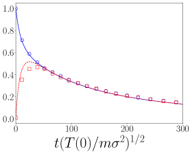
(a)

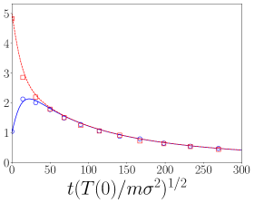
(b)

Figure 13: (Color online) Time evolution of the temperatures for a system of hard spheres (a) and disks (b), as a function of the dimensionless time $\left[\frac{T(0)}{m\sigma^{2}}\right]^{1/2}t$. In both cases, the values of the parameters are $H=29\sigma$ and $\alpha=0.9$. The (blue) circles and the (red) squares are the simulation results for $T$ and $T_{z}$, respectively. The (blue) solid line and (red) dashed lines are the corresponding theoretical prediction obtained by solving numerically Eqs. (33) and (34).

V Discussion and Conclusions

In this work, we have formulated a kinetic equation for a dilute granular system composed of inelastic hard spheres or disks that are confined between two vertically vibrating walls separated a distance larger than twice the diameter of the particles. The equation for the one-particle distribution function has the typical free-streaming part and the collisional contribution that takes into account the particle-particle and the particle-wall collisions. The particle-particle collisional term takes into account the effects of the confinement by restricting the orientation of collisions to such in which the two particles involved are inside the system. The spatial domain of the system is naturally divided into the “bulk” part (in which all the orientations of the collisions are allowed) plus the “boundary” part closed to the walls (where the orientation of the collisions are restricted). Although the kinetic equation makes sense for arbitrary height, $H$, we have restricted ourselves to small enough heights so that the assumption that the distribution function is $z$-independent is expected to be valid. In this case, a closed evolution equation for the marginal distribution, $f(\bm{r}_{\parallel},\bm{v},t)\equiv\frac{1}{(H-\sigma)}\int_{\sigma/2}^{H-\sigma/2}\differential{z}\leavevmode\nobreak\ f(\bm{r},\bm{v},t)$, is obtained and, remarkably, the particle-particle collisions contribution splits into two terms: one corresponding to an ultra-confined system of height $2\sigma$, plus other corresponding to a bulk system (there are not restrictions on the orientation of the collisions) of height $H-2\sigma$.

Considering that there are not gradients in the horizontal direction, the kinetic equation is solved by assuming that the distribution function is a gaussian with two temperatures (the horizontal and vertical temperatures). Closed evolution equations for the partial temperatures are obtained, that are explicitly written in the linear in $\beta\equiv\frac{T_{z}}{T}-1$ approximation, Eqs. (33) and (34). The structure of the equations is transparent: energy is injected in the vertical direction due to the walls and it is transferred to the horizontal direction through collisions. Energy is dissipated in particle-particle collisions that is reflected in both equations. The equations admit a stationary state in which the energy lost in collisions is compensated by the energy injected by the particle-wall collisions. Moreover, we have shown that this solution is linearly stable. The temperature quotient in the stationary state, $\beta_{s}$, is always positive (indicating that $T_{z,s}>T_{s}$) and decays monotonically with $\alpha$, vanishing in the elastic limit (consistently with equipartition). On the other hand, the horizontal temperature, $T_{s}$, decays with the height (consistently with the fact that there are less particle-wall collisions with respect to particle-particle collisions) and increases with $\alpha$, as expected. While $\beta_{s}$ is density independent, $T_{s}\sim(n\sigma^{d})^{-2}$. This behavior can be intuitively understood from the fact that energy injection comes from particle-wall collisions and goes with $n\sigma^{d}$, while dissipation comes from particle-particle collisions that goes with $(n\sigma^{d})^{2}$. The theoretical predictions that comes from Eqs. (33) and (34) agree very well with MD simulation results for a wide range of the parameters. We have shown that for mild inelasticities, let us say $0.8<\alpha<1$, the agreement is excellent, both for the stationary values and for the dynamics. For stronger inelasticities, the agreement is also very good when the equations beyond the linear approximation in $\beta$ are numerically solved. All these results give a strong support to the kinetic theory developed in the paper.

The obtained density dependence of the horizontal stationary temperature is relevant, as the density dependence of the stationary pressure is, then, $p_{s}\sim(n\sigma^{d})^{-1}$. We have already mentioned that the fact that $\frac{dp_{s}}{dn}<0$ is related with the presence of an instability. In fact, in the simulations, clusters were developed for some values of the parameters that, of course, were disregarded in the previous section in order to compare with the theoretical predictions. In Fig. 14, a snapshot of a hard disks system once the stationary state has been reached is shown. Only a portion of the system close to the region where the inhomogeneities are developed is plotted. The cluster of particles can be clearly seen. The values of the parameters are the ones for hard disks with $H=8\sigma$ and $\alpha=0.85$.

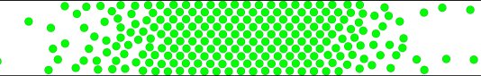
Figure 14: Snapshot of a hard disks system once the stationary state has been reached. Only a portion of the system close to the region where the inhomogeneities are developed is plotted. The values of the parameters are the ones for hard disks with $H=8\sigma$ and $\alpha=0.85$.

Let us remark that this instability is compatible with the fact that the stationary solution of Eqs. (33) and (34) is linearly stable, as in the stability analysis the spatial homogeneity was taken for granted. In order to analyze the nature of the present instability, a similar analysis to the one performed in mgb19b could be done, i.e., to perform a linear stability analysis of the homogeneous state by assuming a hydrodynamic description in the plane. Nevertheless, in Ref. mgb19b it was clear that the two-dimensional transport coefficients should be taken (at least for $\varepsilon\ll 1$), whether in our case, it is not so clear. In fact, here it becomes evident that, as long as the kinetic equation for ultra-confined systems bmg16 is the natural tool to tackle the transition from a three-dimensional system to a two-dimensional one, the kinetic equation of the paper, Eq. (5) or Eq. (16), let us study the transition from a confined system to a “pure” three-dimensional system where the “boundary” terms of the kinetic equation are not relevant.

Finally, let us mention that Eqs. (33) and (34) describe the time evolution of the partial temperatures in a very general framework. The only essential ingredient is that the ansatz given by Eq. (24) be approximately valid. Hence, the equations can be the starting point of further studies such as the study of the Kovacs pt14 ; bgmb14 or Mpemba lvps17 effects. The difference with the models of the above mentioned references is that, in our context, the variables involved in the process can be controlled and the effects can be experimentally relevant. In bpr22 , the Mpemba effect is studied in a more similar model in which the energy is injected anisotropically, although it is hard to perform a direct comparison between the results for both models as the energy injection mechanisms are different (it is stochastic in the case of bpr22 , while it is deterministic in ours). Beyond these transient effects, from Eqs. (33) and (34), it would also be possible to analyze if, before the stationary state is reached, a universal state (in the sense that it is independent of the initial condition) is reached in the long-time limit as it happens in other granular systems gmt12 ; bmgb14 . This point is specially relevant if a hydrodynamic in the plane description is possible. Work in these lines is in progress.

Appendix A Properties of the particle-wall collision term

In this appendix we will proof the relations (24), and (25). To do that, we start using the expression of the operator $L_{\uparrow}$ defined in (10) in order to develop explicitly the left hand side of (24)

$$\begin{aligned} \int\differential\bm{v}\psi(\bm{v})L_{\uparrow}f(\bm{v},t)=&\int\differential\bm{v}\psi(\bm{v})\left[\Theta(-v_{z}-2v_{p})|2v_{p}+v_{z}|b_{\uparrow}-\Theta(v_{z})v_{z}\right]f(\bm{v},t),\\ =&\int\differential\bm{v}\psi(\bm{v})\Theta(b_{\uparrow}v_{z})|b_{\uparrow}v_{z}|f(b_{\uparrow}\bm{v},t)-\int\differential\bm{v}\psi(\bm{v})\Theta(v_{z})v_{z}f(\bm{v},t),\end{aligned}$$ (53)

when we use the definition of $b_{\uparrow}$ operator. Making a change of variable ${\bm{u}}\equiv b_{\uparrow}{\bm{v}}$ in the first integral of the right hand site, and taking into account that the jacobian is the unity, we have

$$\begin{aligned} \int\differential\bm{v}\psi(\bm{v})L_{\uparrow}f(\bm{v},t)=&\int\differential\bm{u}\psi(b_{\uparrow}\bm{u})\Theta(u_{z})|u_{z}|f(\bm{u},t)-\int\differential\bm{v}\psi(\bm{v})\Theta(v_{z})v_{z}f(\bm{v},t),\\ =&\int\differential\bm{v}f(\bm{v},t)\absolutevalue{v_{z}}\Theta(v_{z})(b_{\uparrow}-1)\psi(\bm{v}).\end{aligned}$$ (54)

Note that the property $b_{\uparrow}^{-1}=b_{\uparrow}$ is used in the last equality. Using the same steps, the expression (25) is obtained.

Appendix B Evaluation of the collision integrals

The objective in this Appendix is to calculate the particle-particle collision contribution to the evolution equations of the partial temperatures. Taking into account Eq. (III) and

$$\begin{aligned} (b_{\widehat{\bm{\sigma}}}-1)(v_{z}^{2}+v_{1z}^{2})=&v_{z}^{\prime 2}+v_{1z}^{\prime 2}-v_{z}^{2}-v_{1z}^{2},\\ =&\frac{(\alpha+1)^{2}}{2}(\bm{g}\cdot\widehat{\bm{\sigma}})^{2}\widehat{\sigma}_{z}^{2}-(\alpha+1)(\bm{g}\cdot\widehat{\bm{\sigma}})\widehat{\sigma}_{z}g_{z},\end{aligned}$$ (55)

we have

$$\begin{aligned} \frac{1}{H-\sigma}\int_{\sigma/2}^{H-\sigma/2}dz\int\differential\bm{v}v_{z}^{2}\mathcal{J}_{z}[f|f]=\frac{\sigma^{d-1}(\alpha+1)}{2(H-\sigma)}\int_{\sigma/2}^{H-\sigma/2}\differential z\int\differential\bm{v}_{1}\int\differential\bm{v}f(\bm{v}_{1},t)f(\bm{v},t)\\ \int_{\Omega_{d}(H,z)}\differential\widehat{\bm{\sigma}}\absolutevalue{\bm{g}\cdot\widehat{\bm{\sigma}}}\Theta(\bm{g}\cdot\widehat{\bm{\sigma}})\left[\frac{(\alpha+1)}{2}(\bm{g}\cdot\widehat{\bm{\sigma}})^{2}\widehat{\sigma}_{z}^{2}-(\bm{g}\cdot\widehat{\bm{\sigma}})\widehat{\sigma}_{z}g_{z}\right]\\ =\frac{\sigma^{d-1}(\alpha+1)}{2(H-\sigma)}\int_{\sigma/2}^{H-\sigma/2}\differential z\int\differential\bm{v}_{1}\int\differential\bm{v}f(\bm{v}_{1},t)f(\bm{v},t)\int_{\Omega_{d}(H,z)}\differential\widehat{\bm{\sigma}}\absolutevalue{\bm{g}\cdot\widehat{\bm{\sigma}}}\Theta(-\bm{g}\cdot\widehat{\bm{\sigma}})\\ \left[\frac{(\alpha+1)}{2}(\bm{g}\cdot\widehat{\bm{\sigma}})^{2}\widehat{\sigma}_{z}^{2}-(\bm{g}\cdot\widehat{\bm{\sigma}})\widehat{\sigma}_{z}g_{z}\right],\end{aligned}$$ (56)

where we have changed the labels $\bm{v}\leftrightarrow\bm{v}_{1}$ in the last step. In this way, we can integrate over all values of $\bm{v}_{1}$ and $\bm{v}$ (without the restriction coming from $\Theta$) and we have

$$\begin{aligned} \frac{1}{H-\sigma}\int_{\sigma/2}^{H-\sigma/2}dz\int\differential\bm{v}v_{z}^{2}\mathcal{J}_{z}[f|f]=\frac{\sigma^{d-1}(\alpha+1)}{4(H-\sigma)}\int_{\sigma/2}^{H-\sigma/2}\differential z\left[\frac{(\alpha+1)}{2}H_{1}(z)-H_{2}(z)\right],\end{aligned}$$ (57)

with

$$H_{1}(z) \equiv \int\differential\bm{v}_{1}\int\differential\bm{v}f(\bm{v}_{1},t)f(\bm{v},t)\int_{\Omega_{d}(H,z)}\differential\widehat{\bm{\sigma}}\absolutevalue{\bm{g}\cdot\widehat{\bm{\sigma}}}^{3}\widehat{\sigma}_{z}^{2},$$ (58)

$$H_{2}(z) \equiv \int\differential\bm{v}_{1}\int\differential\bm{v}f(\bm{v}_{1},t)f(\bm{v},t)\int_{\Omega_{d}(H,z)}\differential\widehat{\bm{\sigma}}\absolutevalue{\bm{g}\cdot\widehat{\bm{\sigma}}}(\bm{g}\cdot\widehat{\bm{\sigma}})\widehat{\sigma}_{z}g_{z}.$$ (59)

Let us first calculate the contribution coming from $H_{1}(z)$. Taking into account the shape of the distribution function given by Eq. (24), we make the change of variables

$$\bm{C} =\frac{1}{2}(\bm{k}+\bm{k}_{1}),$$ (60)

$$\bm{c} =\bm{k}_{1}-\bm{k},$$ (61)

where

$$\bm{k} =\frac{v_{x}}{w}\widehat{\bm{e}}_{x}+\frac{v_{y}}{w}\widehat{\bm{e}}_{y}+\frac{v_{z}}{w_{z}}\widehat{\bm{e}}_{z},$$ (62)

$$\bm{k}_{1} =\frac{v_{1x}}{w}\widehat{\bm{e}}_{x}+\frac{v_{1y}}{w}\widehat{\bm{e}}_{y}+\frac{v_{1z}}{w_{z}}\widehat{\bm{e}}_{z},$$ (63)

for $d=3$ and

$$\bm{k} =\frac{v_{y}}{w}\widehat{\bm{e}}_{y}+\frac{v_{z}}{w_{z}}\widehat{\bm{e}}_{z},$$ (64)

$$\bm{k}_{1} =\frac{v_{1y}}{w}\widehat{\bm{e}}_{y}+\frac{v_{1z}}{w_{z}}\widehat{\bm{e}}_{z},$$ (65)

for $d=2$. Note that the jacobian of transformation is $\absolutevalue{\mathbb{J}}=w^{2(d-1)}w_{z}^{2}$. Taking into account Eq (24), $f(\bm{v}_{1},t)f(\bm{v},t)$ is expressed in the new variables

$$f(\bm{v}_{1},t)f(\bm{v},t)=\Bigg{[}\frac{n}{\pi^{\frac{d}{2}}w^{d-1}(t)w_{z}(t)}\Bigg{]}^{2}\exp(-2C^{2})\exp(-\frac{1}{2}c^{2}).$$ (66)

In these variables, $H_{1}(z)$ is expressed as

$$\begin{split}H_{1}(z)=\Bigg{(}\frac{n}{\pi^{\frac{d-1}{2}}}\Bigg{)}^{2}\int\differential\bm{C}\exp(-2C^{2})\int\differential\bm{c}\exp(-\frac{1}{2}c^{2})\int_{\Omega_{d}(H,z)}\differential\widehat{\bm{\sigma}}\absolutevalue{\bm{c}\cdot\widehat{\bm{a}}}^{3}\\ \Big{[}(w\widehat{\sigma}_{\parallel})^{2}+(w_{z}\widehat{\sigma}_{z})^{2}\Big{]}^{3/2}\sigma_{z}^{2},\end{split}$$ (67)

where $\widehat{\sigma}_{\parallel}\equiv|\widehat{\bm{\sigma}}-\widehat{\sigma}_{z}\widehat{e}_{z}|$ and $\widehat{\bm{a}}$ is a unitary vector in the direction of $w\widehat{\sigma}_{x}\widehat{\bm{e}}_{x}+w\widehat{\sigma}_{y}\widehat{\bm{e}}_{y}+w_{z}\widehat{\sigma}_{z}\widehat{\bm{e}}_{z}$ or $w\widehat{\sigma}_{y}\widehat{\bm{e}}_{y}+w_{z}\widehat{\sigma}_{z}\widehat{\bm{e}}_{z}$ for $d=3$ and $d=2$ respectively. The integral in $\bm{C}$ is trivial

$$\int\differential\bm{C}\exp(-2C^{2})=\left(\frac{\pi}{2}\right)^{d/2},$$ (68)

and the integral in $\bm{c}$ is

$$\int\differential\bm{c}\exp(-\frac{1}{2}c^{2})\absolutevalue{\bm{c}\cdot\widehat{\bm{a}}}^{3}=4(2\pi)^{\frac{d-1}{2}},$$ (69)

where we have used that the integral does not depend on $\widehat{\bm{a}}$. In this way Eq. (67) reduces to

$$\begin{aligned} H_{1}(z)=&\frac{2\sqrt{2}n^{2}w^{3}}{\sqrt{\pi}}\int_{\Omega_{d}(H,z)}\differential\widehat{\bm{\sigma}}\left[\widehat{\sigma}_{\parallel}^{2}+\widehat{\sigma}_{z}^{2}+\left(\frac{w_{z}^{2}}{w^{2}}-1\right)\widehat{\sigma}_{z}^{2}\right]^{3/2}\sigma_{z}^{2},\\ =&\frac{2\sqrt{2}n^{2}w^{3}}{\sqrt{\pi}}\int_{\Omega_{d}(H,z)}\differential\widehat{\bm{\sigma}}\left(1+\beta\widehat{\sigma}_{z}^{2}\right)^{3/2}\widehat{\sigma}_{z}^{2},\end{aligned}$$ (70)

where we have defined $\beta\equiv(w_{z}^{2}/w^{2}-1)\equiv(T_{z}/T-1)$ and the equality $||\widehat{\bm{\sigma}}||=1$ has been used. Considering spherical coordinates in $d$-dimensions and taking into account the explicit parametrization of the domain $\Omega_{d}(H,z)$, we have

$$\begin{aligned} \frac{1}{(H-\sigma)}\int_{\sigma/2}^{H-\sigma/2}\differential zH_{1}(z)=\frac{2\sqrt{2}n^{2}w^{3}\Omega_{T,d-1}}{\sqrt{\pi}\varepsilon\sigma}\left[I_{1}+\sigma(\varepsilon-1)I_{2}\right],\end{aligned}$$ (71)

where we have defined

$$I_{1}\equiv \int_{\sigma/2}^{3\sigma/2}\differential z\int_{\pi/2-b_{2}(z)}^{\pi/2+b_{1}(z)}\differential\theta\left(1+\beta\cos^{2}\theta\right)^{3/2}\sin^{d-2}\theta\cos^{2}\theta,$$ (72)

$$I_{2}\equiv \int_{0}^{\pi}\differential\theta\left(1+\beta\cos^{2}\theta\right)^{3/2}\sin^{d-2}\theta\cos^{2}\theta.$$ (73)

The first integral defined in Eq. (72) can be simplified by changing variables from $\theta$ to $z_{1}$ defined through

$$\begin{aligned} \cos\theta=\frac{z_{1}-z}{\sigma}.\end{aligned}$$ (74)

It can be expressed as

$$\begin{aligned} I_{1}=&\frac{1}{\sigma}\int_{\sigma/2}^{3\sigma/2}\differential z\int_{\sigma/2}^{3\sigma/2}\differential z_{1}\left[1+\beta\left(\frac{z-z_{1}}{\sigma}\right)^{2}\right]^{3/2}\left[1-\left(\frac{z-z_{1}}{\sigma}\right)^{2}\right]^{(d-3)/2}\left(\frac{z-z_{1}}{\sigma}\right)^{2},\end{aligned}$$ (75)

or, in terms of the dimensionless variables,

$$\tilde{z}_{1}=\frac{z_{1}-\sigma/2}{\sigma},\quad\tilde{z}_{2}=\frac{z-\sigma/2}{\sigma},$$ (76)

as

$$I_{1}=2\sigma\int_{0}^{1}\mathrm{d}\tilde{z}_{1}\int_{0}^{\tilde{z}_{1}}\mathrm{\leavevmode\nobreak\ d}\tilde{z}_{2}\left(1+\beta\tilde{z}_{12}^{2}\right)^{3/2}\left(1-\tilde{z}_{12}^{2}\right)^{(d-3)/2}\tilde{z}_{12}^{2},$$ (77)

where we have introduced $\tilde{z}_{12}\equiv\tilde{z}_{1}-\tilde{z}_{2}$ and we have used that the integrand is invariant under the change $\tilde{z}_{1}$ by $\tilde{z}_{2}$. Finally, changing variables to

$$y=\tilde{z}_{1}-\tilde{z}_{2},\quad Y=\frac{1}{2}\left(\tilde{z}_{1}+\tilde{z}_{2}\right),$$ (78)

it is obtained

$$\begin{aligned} I_{1}=2\sigma\int_{0}^{1}\mathrm{d}y\int_{y/2}^{1-y/2}\mathrm{\leavevmode\nobreak\ d}Y\;y^{2}\left(1-y^{2}\right)^{(d-3)/2}\left(1+\beta y^{2}\right)^{3/2}=&2\sigma\int_{0}^{1}\mathrm{d}y\;y^{2}(1-y)\left(1-y^{2}\right)^{(d-3)/2}\\ &\left(1+\beta y^{2}\right)^{3/2}.\end{aligned}$$ (79)

The integral $I_{2}$ can be expressed in a similar way that $I_{1}$. In effect, by introducing the new variable,

$$\begin{aligned} x=\cos\theta,\end{aligned}$$ (80)

$I_{2}$ can be expressed as

$$I_{2}=\begin{aligned} 2\int_{0}^{1}\differential x\;x^{2}(1-x^{2})^{(d-3)/2}\left(1+\beta x^{2}\right)^{3/2}.\end{aligned}$$ (81)

By introducing Eqs. (79) and (81) into Eq. (71), it is obtained

$$\begin{aligned} \frac{1}{(H-\sigma)}\int_{\sigma/2}^{H-\sigma/2}\differential zH_{1}(z)=&\frac{4\sqrt{2}n^{2}w^{3}\Omega_{T,d-1}}{\sqrt{\pi}\varepsilon}\int_{0}^{1}\differential y\;y^{2}(1-y^{2})^{(d-3)/2}(1+\beta y^{2})^{3/2}[(\varepsilon-1)+(1-y)].\end{aligned}$$ (82)

To get a similar expression for $\frac{1}{(H-\sigma)}\int_{\sigma/2}^{H-\sigma/2}\differential zH_{2}(z)$, we follow similar steps. By changing variables to the ones introduced in equations (60) and (61), we have

$$\begin{split}H_{2}(z)=\left(\frac{n}{\pi^{\frac{d}{2}}}\right)^{2}\int\differential\bm{C}\exp(-2C^{2})\int\differential\bm{c}\exp(-\frac{1}{2}c^{2})\int_{\Omega_{d}(H,z)}d\widehat{\bm{\sigma}}\absolutevalue{\bm{c}\cdot\widehat{\bm{a}}}(\bm{c}\cdot\widehat{\bm{a}})\\ \Big{[}(w\widehat{\sigma}_{\parallel})^{2}+(w_{z}\widehat{\sigma}_{z})^{2}\Big{]}^{1/2}({\bm{c}}\cdot\widehat{\bm{e}}_{z})w_{z}\widehat{\sigma}_{z}.\end{split}$$ (83)

Expressing the variable $\bm{c}$ in orthonormal basis with components $\{\widehat{\bm{b}}_{1},\dots,\widehat{\bm{b}}_{d-1},\widehat{\bm{a}}\}$ and integrating over $\bm{c}$ and $\bm{C}$, it is obtained

$$H_{2}(z)=\frac{2\sqrt{2}n^{2}w^{3}}{\sqrt{\pi}}(1+\beta)\int_{\Omega_{d}(H,z)}\differential\widehat{\bm{\sigma}}\Big{(}1+\beta\widehat{\sigma}_{z}^{2}\Big{)}^{1/2}\widehat{\sigma}_{z}^{2}.$$ (84)

Integrating over $z$ and expressing Eq. (84) in polar coordinates, we have

$$\begin{aligned} \frac{1}{(H-\sigma)}\int_{\sigma/2}^{H-\sigma/2}\differential zH_{2}(z)=\frac{2\sqrt{2}n^{2}w^{3}\Omega_{T,d-1}(1+\beta)}{\sqrt{\pi}\varepsilon\sigma}\left[I^{*}_{1}+\sigma(\varepsilon-1)I^{*}_{2}\right],\end{aligned}$$ (85)

with

$$I^{*}_{1}\equiv \int_{\sigma/2}^{3\sigma/2}\differential z\int_{\pi/2-b_{2}(z)}^{\pi/2+b_{1}(z)}\differential\theta\left(1+\beta\cos^{2}\theta\right)^{1/2}\sin^{d-2}\theta\cos^{2}\theta,$$ (86)

$$I^{*}_{2}\equiv \int_{0}^{\pi}\differential\theta\left(1+\beta\cos^{2}\theta\right)^{1/2}\sin^{d-2}\theta\cos^{2}\theta.$$ (87)

Using the same variables as above, we can express $I^{*}_{1}$ and $I^{*}_{2}$ as a function of $y$ as

$$\begin{aligned} I^{*}_{1}=&2\sigma\int_{0}^{1}\mathrm{d}y\;y^{2}(1-y)\left(1-y^{2}\right)^{(d-3)/2}\left(1+\beta y^{2}\right)^{1/2},\\ I^{*}_{2}=&2\int_{0}^{1}\differential y\;y^{2}(1-y^{2})^{(d-3)/2}\left(1+\beta y^{2}\right)^{1/2},\end{aligned}$$ (88)

and, by introducing this results into Eq. (85), we have

$$\begin{aligned} \frac{1}{(H-\sigma)}\int_{\sigma/2}^{H-\sigma/2}\differential zH_{2}(z)=&\frac{4\sqrt{2}n^{2}w^{3}\Omega_{T,d-1}(1+\beta)}{\sqrt{\pi}\varepsilon}\int_{0}^{1}\differential y\;y^{2}(1-y^{2})^{(d-3)/2}(1+\beta y^{2})^{1/2}[(\varepsilon-1)+(1-y)].\end{aligned}$$ (89)

Finally, by introducing Eqs. (82) and (89) into Eq. (57), the particle-particle collisional contribution to the vertical temperature equation, i.e. Eq. (31), is obtained.

Following similar steps, the corresponding contribution to the horizontal temperature is obtained.

References

- (1) I. Goldhirsch, Rapid Granular Flows, Annu. Rev. Fluid Mech. 35, 57 (2003).
- (2) I. S. Aranson and L. S. Tsimring, Patterns and collective behavior in granular media: theoretical concepts, Rev. Mod. Phys. 78, 641 (2006).
- (3) N. V. Brilliantov and T. Pöschel,Kinetic theory of granular gases (Oxford University Press on Demand, 2004).
- (4) V. Garzó, Granular Gaseous Flows (Springer Nature, Cham, 2019).
- (5) A. Prevost, D. A. Egolf, and J. S. Urbach, Forcing and Velocity Correlations in a Vibrated Granular Monolayer, Phys. Rev. Lett. 89, 084301 (2002).
- (6) J. S. Olafsen and J. S. Urbach, Two-Dimensional Melting Far from Equilibrium in a Granular Monolayer, Phys. Rev. Lett. 95, 098002 (2005).
- (7) P. Melby, F. Vega Reyes, A. Prevost, R. Robertson, P. Kumar, D. A. Egolf, and J. S. Urbach, The dynamics of thin vibrated granular layers, J. Phys.: Condens. Matter 17 (2005) S2689-S2704.
- (8) G. Castillo, N. Mújica, and R. Soto, Fluctuations and Criticality of a Granular Solid-Liquid-Like Phase Transition, Phys. Rev. Lett. 109, 095701 (2012).
- (9) B. Néel, I. Rondini, A. Turzillo, N. Mujica, and R. Soto, Dynamics of a first-order transition to an absorbing state, Phys. Rev. E 89, 042206 (2014).
- (10) G. Castillo, N. Mújica, and R. Soto, Universality and criticality of a second-order granular solid-liquid-like phase transition, Phys. Rev. E 91, 012141 (2015).
- (11) M. Guzmán and R. Soto, Critical phenomena in quasi-two-dimensional vibrated granular systems, Phys. Rev. E 97, 012907 (2018).
- (12) J. J. Brey, J. W. Dufty, C. S. Kim, and A. Santos, Hydrodynamics for a granular flow at low density, Phys. Rev. E 58, 4638 (1998).
- (13) R. Brito, D. Risso, and R. Soto, Hydrodynamic modes in a confined granular fluid, Phys. Rev. E 87, 022209 (2013).
- (14) P. Maynar, M. I. García de Soria, and J. J. Brey, Homogeneous dynamics in a vibrated granular monolayer, J. Stat. Mech. (2019) 093205.
- (15) P. Maynar, M. I. García de Soria, and J. J. Brey, Understanding an instability in vibrated granular monolayers, Phys. Rev. E 99, 032903 (2019).
- (16) P. Maynar, M. I. García de Soria, and J. J. Brey, Dynamics of an inelastic tagged particle under strong confinement, Phys. Fluids 34, 123321 (2022).
- (17) J. J. Brey, P. Maynar, M. I. García de Soria, Kinetic equation and nonequilibrium entropy for a quasi-two-dimensional gas, Phys. Rev. E 94, 040103(R) (2016).
- (18) J. J. Brey, M. I. García de Soria, and P. Maynar, Boltzmann kinetic equation for a strongly confined gas of hard spheres, Phys. Rev. E 96, 042117 (2017).
- (19) M. Mayo, J. J. Brey, M. I. García de Soria, and P. Maynar, Kinetic Theory of a confined quasi-one-dimensional gas of hard disks, Physica A 597 (2022) 127237.
- (20) P. Maynar, M. I. García de Soria, and J. J. Brey, The Enskog Equation for Confined Elastic Hard Spheres, J. Stat. Phys. 170, 999 (2018).
- (21) K. Roeller, J. P. D. Clewett, R. M. Bowley, S. Herminghaus, and M. R. Swift, Liquid-Gas Phase Separation in Confined Vibrated Dry Granular Matter, Phys. Rev. Lett. 107, 048002 (2011).
- (22) J. P. D. Clewett, K. Roeller, R. M. Bowley, S. Herminghaus, and M. R. Swift, Emergent Surface Tension in Vibrated, Noncohesive Granular Media, Phys. Rev. Lett. 109, 228002 (2012).
- (23) J. P. D. Clewett, J. Wade, R. M. Bowley, S. Herminghaus, M. R. Swift, and M. G. Mazza, The minimization of mechanical work in vibrated granular matter, Sci. Rep. 6, 28726 (2016).
- (24) P. Résibois and M. de Leener, Classical kinetic theory of fluids (Wiley, 1977).
- (25) J. R. Dorfman, H. van Beijeren, and T. R. Kirkpatrick, Contemporary kinetic theory of matter (Cambridge University Press, 2021).
- (26) J. McLennan and M. A, Introduction to nonequilibrium statistical mechanics (Prentice Hall, 1989).
- (27) T. Van Noije and M. Ernst, Velocity distributions in homogeneous granular fluids: the free and the heated case, Granular Matter 1, 57-64 (1998).
- (28) J. J. Brey, M. I. García de Soria, and P. Maynar, Inhomogeneous cooling state of a strongly confined granular gas at low density, Phys. Rev. E 100, 052901 (2019).
- (29) M. Mayo, M. I. García de Soria, and P. Maynar, to be published.
- (30) M. P. Allen and D. J. Tisdesley, Computer Simulations of Liquids (Oxford Science Publications, New York, 1987).
- (31) A. Prados and E. Trizac, Kovacs-like memory effect in driven granular gases, Phys. Rev. Lett. 112, 198001 (2014).
- (32) J. J. Brey, M. I. García de Soria, P. Maynar, and V. Buzón, Memory effects in the relaxation of a confined granular gas, Phys. Rev. E 90, 032207 (2014).
- (33) A. Lasanta, F. Vega Reyes, A. Prados, and A. Santos, When the hotter cools more quickly: Mpemba effect in granular fluids, Phys. Rev. Lett. 119, 148001 (2017).
- (34) A. Biswas, V. V. Prasad, and R. Rajesh, Mpemba Effect in Anisotropically Driven Inelastic Maxwell Gases, J. Stat. Phys. 186, 45 (2022).
- (35) M. I. García de Soria, P. Maynar, and E. Trizac, Universal reference state in a driven homogeneous granular gas, Phys. Rev. E 85, 051301 (2012).
- (36) J. J. Brey, P. Maynar, M. I. García de Soria, and V. Buzón, Homogeneous hydrodynamics of a collisional model of confined granular gases, Phys. Rev. E 89, 052209 (2014).