Ab initio derivation of generalised hydrodynamics
from a gas of interacting wave packets

Abstract

Hydrodynamics is an efficient theory for describing the large-scale dynamics of many-body systems. The equations of hydrodynamics at the Euler scale are often obtained phenomenologically under the assumption of local entropy maximisation. With integrability, this has led to the theory of generalised hydrodynamics (GHD), based on local generalised Gibbs ensembles. But deriving such equations from the microscopic dynamics itself remains one of the most important challenges of mathematical physics. This is especially true in deterministic, interacting particle systems. We provide an ab initio derivation of the GHD equations in the Lieb-Liniger quantum integrable model describing cold atomic gases in one dimension. The derivation is valid at all interaction strengths, and does not rely on the assumption of local entropy maximisation. For this purpose, we show that a gas of wave packets, formed by macroscopic-scale modulations of Bethe eigenfunctions, behave as a gas of classical particles with a certain integrable dynamics, and that at large scales, this classical dynamics gives rise to the GHD equations. This opens the way for a much deeper mathematical and physical understanding of the hydrodynamics of integrable models.

Introduction.— In recent years there has been much interest in developing hydrodynamic descriptions of many-body quantum systems in low dimensions Abanov et al. (2021). One such avenues is generalised hydrodynamics (GHD) Castro-Alvaredo et al. (2016); Bertini et al. (2016), a hydrodynamic theory for integrable systems, which accounts for the presence of an extensive number of conserved quantities. GHD applies widely, from “integrable turbulence” Zakharov (2009), including gases of solitons El (2021); Suret et al. (2023), and other classical systems Doyon and Spohn (2017a); Cao et al. (2018); Bastianello et al. (2018); Spohn (2020); Doyon (2019); Bulchandani et al. (2019); Koch and Bastianello (2023), to quantum spin chains, field theories and gases Castro-Alvaredo et al. (2016); Bertini et al. (2016); Doyon et al. (2017); Bulchandani et al. (2017, 2018); Caux et al. (2019); Castro-Alvaredo et al. (2020). GHD has been confirmed experimentally in cold atoms Schemmer et al. (2019); Malvania et al. (2021); Møller et al. (2021), and has seen far-reaching theoretical developments, see the reviews Doyon (2020); Bastianello et al. (2022); Spohn (2023); Essler (2022).

At the Euler scale – where viscous and diffusive effects are scaled away – GHD takes a universal structure. The phase-space density $\rho_{\rm p}(\theta,x,t)$ representing the local state of the system at time $t$ and position $x$, as a function of the “rapidity” $\theta$, satisfies the conservation law Castro-Alvaredo et al. (2016); Bertini et al. (2016)

$$\partial_{t}\rho_{\rm p}(\theta,x,t)+\partial_{x}\big{(}v^{\rm eff}(\theta,x,t)\rho_{\rm p}(\theta,x,t)\big{)}=0.$$ (1)

The current in the second term is set by an “effective velocity” $v^{\rm eff}(\theta,x,t)=v^{\rm eff}_{[\rho_{\rm p}(\cdot,x,t)]}(\theta)$, which depends functionally and nonlinearly on the state at $(x,t)$. In its simplest form, the effective velocity, for some state $\rho(\theta)$, is the solution to the linear integral equation

$$v^{\rm eff}_{[\rho]}(\theta)=\theta+\int{\rm d}\alpha\,\varphi(\theta-\alpha)\rho(\alpha)(v^{\rm eff}_{[\rho]}(\alpha)-v^{\rm eff}_{[\rho]}(\theta))$$ (2)

where $\varphi(\theta-\alpha)$ encodes the interaction (see below). $\rho_{\rm p}(\theta,x,t)$ is a density in the phase space of asymptotic excitations (“particles”) and their momenta $\theta$ (“rapidity”): ${\rm d}\theta{\rm d}x\,\rho_{\rm p}(\theta,x,t)$ is the number of particles with asymptotic momenta in $[\theta,\theta+{\rm d}\theta]$ seen in a time-of-flight thought experiment, where the “fluid cell” at $x,t$, of mesoscopic length ${\rm d}x$, is taken out of the fluid and let to expand in the vacuum. Depending on the model to which GHD is applied, asymptotic excitations may be actual particles, classical solitons, stable quantum quasiparticle excitations, radiative waves, etc. In non-integrable models, the dependence on $\theta$ is restricted to certain functions depending on a few parameters such as the temperature (e.g. the black-body radiation). In integrable models, instead, a full space of functions of $\theta$ is available, because all momenta are preserved in scattering events (elastic scattering) Smirnov (1992); Mussardo (2010). We note that it is now possible Malvania et al. (2021), by time-of-flight methods in cold atom gases, to experimentally access (an approximation of) $\rho_{\rm p}(\theta,x,t)$.

Where does (1) come from? In the quantum context, beyond non-interacting models Fagotti (2020); Granet (2023), GHD is derived phenomenologically Castro-Alvaredo et al. (2016); Bertini et al. (2016). Like for most hydrodynamic equations, this relies on the hydrodynamic assumption: in every fluid cell, entropy is independently maximised with respect to the available extensive conserved quantities. Euler-scale hydrodynamic equations are the associated conservation laws, written under this assumption. With integrability, there are infinitely many, and generalised Gibbs ensembles (see the reviews in Calabrese et al. (2016)) are the entropy-maximised states. The Bethe ansatz structure allows one to recast the infinitely-many equations into (1); expressions for average currents (first derived in Castro-Alvaredo et al. (2016)) are the crucial results, see the reviews Borsi et al. (2021); Cubero et al. (2021).

But the hydrodynamic assumption is rather strong. Local relaxation is a many-body effect that is still far from being fully understood. Hydrodynamics is a non-trivial emergent behaviour, and obtaining hydrodynamic equations from the microscopic dynamics, rigorously or with solid arguments, largely remains an outstanding problem of mathematical physics. Eq. (1) has been proved in hard-rod gases Boldrighini et al. (1983); Ferrari et al. (2022) and certain cellular automata Ferrari et al. (2021); Croydon and Sasada (2020) by using “contraction maps”, and in soliton gases by using Whitham modulation theory El (2003); El and Tovbis (2020). But, although quantum integrability admits a rich mathematical structure Faddeev (1996); Mussardo (2010), up to now the available methods appear not to be enough in this context. Deriving (1) without the hydrodynamic assumption in interacting quantum integrable systems remains, since the inception of GHD, a crucial open problem.

In this paper, we solve this problem for the paradigmatic repulsive Lieb-Liniger (LL) model Lieb and Liniger (1963), which describes cold atomic gases (see the reviews Bouchoule and Dubail (2022); Mistakidis et al. (2022)). The principles are expected to apply to Bethe ansatz integrable models more generally. The method combines large-scale amplitude modulations of the Bethe wave function, akin to Whitham’s modulation theory (see the review Grava (2016)), and a scattering map similar to what is used in hard-rod gases (see the book Spohn (2012)).

Our derivation clarifies the underlying physics of Eq. (1): its kinetic interpretation, inspired by factorised scattering theory Zamolodchikov and Zamolodchikov (1979); Novikov et al. (1984); Faddeev and Takhtajan (1987); Smirnov (1992); Mussardo (2010). As proposed in El and Kamchatnov (2005) for soliton gases, and in Doyon et al. (2018a) for quantum integrable models, Eq. (2) arises if $v^{\rm eff}_{[\rho]}(\theta)$ is interpreted as the velocity of a test particle seen on large scales within a gas of density $\rho$, as if it were interacting with other particles simply by accumulating two-body scattering displacements $\varphi(\theta-\alpha)$ (Wigner shifts). Somewhat surprisingly, in quantum systems, the latter is to be taken as the semiclassical spatial shift that wave packets experience in isolated scattering events Doyon et al. (2018a). $v^{\rm eff}$ arises naturally from the Bethe ansatz as a propagation velocity Bonnes et al. (2014), but the question remains: the many-body wave function is extremely complex, why is it sufficient to take a semiclassical shift in order to fully account for the large-scale motion at finite densities?

Our derivation explains this quantum-classical correspondence: a large-scale amplitude modulation is in fact a gas of interacting wave packets, which, by a semiclassical analysis, follow an effective classical dynamics that agrees with the kinetic interpretation. This dynamics is itself integrable Doyon et al. , and gives rise to the GHD equations. In slowly-varying states with finite particle density, wave packets have large, macroscopic spatial extents, and overlap and deform each other. But crucially, we argue that the semiclassical form of their interaction and dynamics is nevertheless valid, albeit “in the large-deviation sense” only – which is sufficient to describe the Euler scale.

The model.— The LL model is a gas of $N$ bosonic particles on the line with repulsive contact interaction,

$$\hat{H}=-\sum_{j=1}^{N}\frac{1}{2}\frac{\partial^{2}}{\partial x_{j}^{2}}+\sum_{(i\neq j)=1}^{N}\frac{c}{2}\delta(x_{i}-x_{j}),\quad c>0.$$ (3)

Its GHD equation (1), with $\varphi(\theta)=2c/(\theta^{2}+c^{2})$ in (2), was proposed in Castro-Alvaredo et al. (2016). The model is Bethe ansatz integrable. Its “eigenfunctions” on the line, or scattering states, are $\Psi_{\bm{\theta}}^{\rm B}(\bm{x})=s(\bm{x})\Psi_{\bm{\theta}}(\bm{x})$ with $s(\bm{x})=\prod_{i<j}\operatorname{sgn}(x_{ij})$ and fermionic-statistics wave functions $\Psi_{\bm{\theta}}(\bm{x})=c_{N}\sum_{\sigma\in S_{N}}(-1)^{|\sigma|}e^{{\rm i}\Phi_{\bm{\theta}}(\bm{x}_{\sigma})}$ where $c_{N}=1/\sqrt{N!(2\pi)^{N}}$, see Gaudin (2014) and (SM, , Sec 1) (here and below, $x_{ij}=x_{i}-x_{j}$, $(\bm{x}_{\sigma})_{i}=x_{\sigma(i)}$ for $\sigma\in S_{N}$ a permutation of $N$ elements, $|\sigma|$ is the order of the permutation). The phase $e^{{\rm i}\Phi_{\bm{\theta}}(\bm{x}_{\sigma})}$ encodes both the free evolution of the particles between interactions, and their scattering, a product of two-body scattering phases,

$$\Phi_{\bm{\theta}}(\bm{x})=\bm{\theta}\cdot\bm{x}+\frac{1}{4}\sum_{i,j}\phi(\theta_{ij})\operatorname{sgn}(x_{ij}),\quad\phi(\theta)=2\operatorname{Arctan}\frac{\theta}{c}.$$ (4)

These states diagonalise the Hamiltonian,

$$\hat{H}\Psi_{\bm{\theta}}(\bm{x})=\frac{\bm{\theta}^{2}}{2}\Psi_{\bm{\theta}}(\bm{x}).$$ (5)

The semiclassical shift is $\varphi(\theta)=\partial_{\theta}\phi(\theta)$; the scattering of two wave packets, where $\varphi(\theta)$ appears as the Wigner shift, is worked out for instance in Bouchoule and Dubail (2022). The scattering states are orthonormal, $\langle\Psi_{\bm{\theta}}^{\rm B}|\Psi_{\bm{\theta}^{\prime}}^{\rm B}\rangle=\delta(\bm{\theta}-\bm{\theta}^{\prime})$ ($\bm{\theta},\bm{\theta}^{\prime}\in{\mathbb{R}}^{N}_{>}$) for ordered rapidities ${\mathbb{R}}^{N}_{>}=\{\bm{\theta}\in{\mathbb{R}}^{N}:\theta_{1}>\theta_{2}>\ldots>\theta_{N}\}$, and span the Hilbert space of symmetric square-integrable functions.

Note that we do not quantise the momenta: the usual Bethe ansatz equations will play no role. This is technically important: in the currently available quantum derivations of GHD, states in fluid cells are described by the thermodynamic Bethe ansatz Yang and Yang (1969); Mossel and Caux (2012), based on quantising momenta with periodic boundary conditions. As fluid cells do not satisfy periodic conditions, this is a (known) logical flaw (recently addressed in free fermionic systems Granet (2023)), which we fully avoid here.

The initial-value problem.— Consider a density matrix $\hat{\varrho}=e^{-\sum_{a}\int{\rm d}x\,\beta_{a}(x)\hat{q}_{a}(x)}$, where $\beta_{a}(x)=\bar{\beta}_{a}(x/L)$ are slowly-varying external fields, with $L$ large, coupled to the local conserved densities $\hat{q}_{a}(x),\,a=0,1,2,\ldots$. The problem is to show that the quantum evolution from this density matrix reproduces GHD. A typical example, implemented in experiments on cold atomic gases Schemmer et al. (2019); Malvania et al. (2021); Møller et al. (2021), is that of a slowly varying chemical potential, $\hat{\varrho}=e^{-\beta\int{\rm d}x\,(\hat{q}_{2}(x)/2-\mu(x)\hat{q}_{0}(x))}$. Here the energy and particles densities are $\hat{q}_{2}(x)/2=\operatorname{He}\sum_{i}\delta(x-\hat{x}_{i})\big{(}\hat{p}_{i}^{2}/2+(c/2)\sum_{j\neq i}\delta(\hat{x}_{i}-\hat{x}_{j})\big{)}$ and $\hat{q}_{0}(x)=\sum_{i}\delta(x-\hat{x}_{i})$ ($\operatorname{He}$ means Hermitian part). To be specific, we look at the evolution of conserved densities. The total conserved charges $\hat{Q}_{a}=\int{\rm d}x\,\hat{q}_{a}(x)$ in the LL model act as $\hat{Q}_{a}\Psi_{\bm{\theta}}^{{\rm B}}(x)=\sum_{j}\theta_{j}^{a}\Psi_{\bm{\theta}}^{{\rm B}}(x)$, and GHD predicts that, for ballistic scaling $(x,t)=(L\bar{x},L\bar{t})$,

$$\lim_{L\to\infty}{\rm Tr}(\hat{\varrho}\,e^{{\rm i}\hat{H}t}\hat{q}_{a}(x)e^{-{\rm i}\hat{H}t})/{\rm Tr}(\hat{\varrho})=\int{\rm d}\theta\,\theta^{a}\rho_{\rm p}(\theta,\bar{x},\bar{t})$$ (6)

in the grand canonical ensemble, where $\rho_{\rm p}(\theta,\bar{x},\bar{t})$ satisfies (1). We are looking to show this prediction of GHD.

Local densities $\hat{q}_{a}(x)$ have, as $a$ increases, complicated but known expressions in terms of $\hat{p}_{i}$’s and $\hat{x}_{i}$’s Davies (1990); Davies and Korepin (2011). However we argue (SM, , Subsec 2.1) that they take the simple form $\hat{q}_{a}(x)=\operatorname{He}\int{\rm d}\theta\,\theta^{a}\hat{\rho}(x,\theta)$ in terms of what we call the empirical density operator $\hat{\rho}(x,\theta)$, which acts on the eigenfunctions $\Psi_{\bm{\theta}}^{\rm B}$ by replacing $e^{{\rm i}\Phi_{\bm{\theta}}(\bm{x})}$ by $\delta(x-x_{i})\delta(\theta-\theta_{i})e^{{\rm i}\Phi_{\bm{\theta}}(\bm{x})}$. This clearly reproduces $\hat{Q}_{a}$; we show that it agrees with $\hat{q}_{0}(x),\,\hat{q}_{2}(x)$ written above and argue that $\int{\rm d}\theta\,\theta^{a}\hat{\rho}(x,\theta)$ are local (SM, , Subsec 2.1). Locality of observables is a crucial technical point: the state of a fluid cell in hydrodynamics describes local observables only. At the Tonks-Girardeau point $c=\infty$, $\hat{\rho}(x,\theta)$ equals the Wigner function usually considered, up to total derivatives (subleading as $L\to\infty$) (SM, , Subsec 2.2). Thus, we are interested in

$$\rho_{\rm p}(\theta,\bar{x},\bar{t})=\lim_{L\to\infty}{\rm Re}\,{\rm Tr}(\hat{\varrho}\,e^{{\rm i}\hat{H}L\bar{t}}\hat{\rho}(L\bar{x},\theta)e^{-{\rm i}\hat{H}L\bar{t}})/{\rm Tr}(\hat{\varrho}).$$ (7)

Other phase-space density operators have been constructed in integrable models Ilievski et al. (2016), but the empirical density operator is the most convenient for our purposes.

Macroscopic modulations and gas of wave packets.— The first step is to study slowly-varying amplitude modulations, and their effective classical dynamics. We will then show how this helps us evaluate (7).

For illustration, consider a single particle with wave function $e^{{\rm i}\theta x}$ of momentum $\theta$ and energy $\theta^{2}/2$. A slowly-varying amplitude modulation is $\bar{A}(x/L)e^{{\rm i}\theta x}$ where $\bar{A}(\bar{x})$ is a fixed rapidly decreasing function Rudin (1991) and $L\gg\theta^{-1}$; the range of significant values of $x$ scales as $O(L)$. By Fourier transform, this is a sharp wave packet around $\theta$: $\bar{A}^{\rm F}(\bar{\alpha})=\int{\rm d}\bar{x}\,\bar{A}(\bar{x})e^{-{\rm i}\bar{\alpha}\bar{x}}/(2\pi)$ is rapidly decreasing, thus the wave function $L\int{\rm d}\alpha\,\bar{A}^{\rm F}(\alpha L)e^{{\rm i}(\theta+\alpha)x}$ spans momenta $\theta+O(L^{-1})$. Large-time evolution, $t=O(L)$, is a linear displacement (up to a phase): using $(\theta+\alpha)^{2}t=\theta^{2}t+2\theta\alpha t+O(L^{-1})$, the time-evolved amplitude is $\bar{A}_{t}(\bar{x})=e^{-{\rm i}\theta^{2}t/2}\bar{A}(\bar{x}_{-t})+O(L^{-1})$ where $\bar{x}_{t}=\bar{x}+\theta t/L$.

We are looking to generalise this simple calculation to the many-body, interacting case. There, a slowly-varying modulation takes the form

$$\Psi_{A}(\bm{x},\bm{\theta})=c_{N}\sum_{\sigma\in S_{N}}(-1)^{|\sigma|}A(\bm{x}_{\sigma},\bm{\theta})\,e^{{\rm i}\Phi_{\bm{\theta}}(\bm{x}_{\sigma})}$$ (8)

where $A(\bm{x},\bm{\theta})=\bar{A}(\bm{x}/L,\bm{\theta})$ with $\bar{A}(\bar{\bm{x}},\bm{\theta})$ rapidly decreasing in both $\bar{\bm{x}}$ and $\bm{\theta}$. The range of significant values are $x_{i}=L\bar{x}_{i}=O(L)$ and $\theta_{i}=O(1)$. Now, however, we must be careful with the scaling: in the grand-canonical ensemble, dominant terms will be for $N\to\infty$ with finite density, $N/L=\nu$ fixed. Thus, we must simultaneously take $L$ and the number of particles large.

We first introduce the “Bethe-Fourier transform”: the nonlinear change of coordinates $A^{\rm B}(\bm{y}^{\bm{\theta}}(\bm{x}),\bm{\theta})=A(\bm{x},\bm{\theta})$ under the “Bethe scattering map”

$$y_{i}=y^{\bm{\theta}}_{i}(\bm{x}):=\frac{\partial\Phi_{\bm{\theta}}}{\partial\theta_{i}}=x_{i}+\frac{1}{2}\sum_{j\neq i}\varphi(\theta_{ij})\operatorname{sgn}(x_{ij}),$$ (9)

followed by the Fourier transform $A^{\rm B}\mapsto A^{\rm BF}$, so that

$$A(\bm{x},\bm{\theta})=\int{\rm d}^{N}\alpha\,A^{\rm BF}(\bm{\alpha},\bm{\theta})e^{{\rm i}\bm{\alpha}\cdot\bm{y}^{\bm{\theta}}(\bm{x})}.$$ (10)

We will refer to $y_{i}$’s as the “free coordinates”. These are still macroscopic, $y_{i}=O(L)$, because the second term in (9) is bounded in magnitude by $N/c=\nu L/c$. The Bethe scattering map is a highly nonlinear change of coordinates (analysed in (SM, , Subsec 3.1)). Nevertheless we argue (SM, , Subsec 3.2) that $\bar{A}^{\rm B}(\bar{\bm{y}},\bm{\theta})=A^{\rm B}(\bar{\bm{y}}L,\bm{\theta})$ is nice enough in $\bar{\bm{y}}$, so that its Fourier transform $\bar{A}^{\rm BF}(\bar{\bm{\alpha}},\bm{\theta})=L^{-N}A^{\rm BF}(\bar{\bm{\alpha}}/L,\bm{\theta})$ can be considered to be rapidly decreasing in $\bar{\bm{\alpha}}$. Therefore $A^{\rm BF}(\bm{\alpha},\bm{\theta})$ is essentially supported on $\alpha_{i}=O(L^{-1})$.

Taylor expanding and taking into account that there are $N\propto L$ particles, $\Phi_{\bm{\theta}+\bm{\alpha}}(\bm{x})=\Phi_{\bm{\theta}}(\bm{x})+\bm{\alpha}\cdot\bm{y}^{\bm{\theta}}(\bm{x})+O(1)$. In contrast to the single-particle case, the correction term is non-vanishing as $L\to\infty$: this is an important phenomenon due to the finite density. Then, the results obtained will be valid not up to vanishing terms, but in the “large-deviation” sense: equality of the exponential divergences, denoted as $a\asymp b\Leftrightarrow\lim_{N\to\infty}N^{-1}(\log a-\log b)=0$. A large-deviation analysis (SM, , Subsec 3.3) implies the decomposition $A(\bm{x},\bm{\theta})e^{{\rm i}\Phi_{\bm{\theta}}(\bm{x})}=\int{\rm d}^{N}\alpha\,C_{A}(\bm{\alpha},\bm{\theta})e^{{\rm i}\Phi_{\bm{\theta}+\bm{\alpha}}(\bm{x})}$ with $C_{A}(\bm{\alpha},\bm{\theta})\asymp A^{\rm BF}(\bm{\alpha},\bm{\theta})$. Thus, the slowly-varying modulation (8) decomposes into a small rapidity shell around $\bm{\theta}$, with the Bethe-Fourier transform as coefficients,

$$\Psi_{A}(\bm{x},\bm{\theta})=\int{\rm d}^{N}\alpha\,C_{A}(\bm{\alpha},\bm{\theta})\Psi_{\bm{\theta}+\bm{\alpha}}(\bm{x}),\quad C_{A}\asymp A^{\rm BF}.$$ (11)

This allows us to interpret $\Psi_{A}(\bm{x},\bm{\theta})$ as a finite-density gas of interacting wave packets. Wave packets are sharp around rapidities $\theta_{i}$’s and of macroscopic spatial extent $\propto L$. Because of the finite density and macroscopic spatial extents, there is a large amount of spatial overlap, where wave packets interact. At the large-deviation level, the interaction is fully encoded within the BF transform.

Time evolution.— For arbitrary $A(\bm{x},\bm{\theta})$, the form (8) is just a generic way of writing a wave function, so there is $A_{t}(\bm{x},\bm{\theta})$ such that $e^{-{\rm i}Ht}\Psi_{A}(\bm{x},\bm{\theta})=\Psi_{A_{t}}(\bm{x},\bm{\theta})$. This is in fact not unique because of the sum over permutations in (8), but we just make a sensible choice. Time evolution to macroscopic times $t=L\bar{t}$ is obtained much like the single free particle case, by using (5) and $(\bm{\theta}+\bm{\alpha})^{2}t/2=\bm{\theta}^{2}t/2+\bm{\theta}\cdot{\bm{\alpha}}\,t+O(1)$, hence $\bar{A}_{t}^{\rm BF}(\bar{\bm{\alpha}},\bm{\theta})\asymp\omega_{t}\bar{A}^{\rm BF}(\bar{\bm{\alpha}},\bm{\theta})e^{-{\rm i}\bm{\theta}\cdot\bar{\bm{\alpha}}\,\bar{t}}$ where $\omega_{t}=e^{-{\rm i}\bm{\theta}^{2}t/2}$. By the inverse Bethe-Fourier transform, we obtain the desired macroscopic-time evolution: $A_{t}(\bm{x},\bm{\theta})=A(\bm{x}_{-t},\bm{\theta})$. The free coordinates evolve linearly, $\bm{y}_{t}=\bm{y}+\bm{\theta}t$, and $\bm{x}_{t}$ follow interacting trajectories, solving $\bm{y}^{\bm{\theta}}(\bm{x}_{t})=\bm{y}_{t}$. That is, our main result is that

$$e^{-{\rm i}Ht}\Psi_{A}(\bm{x},\bm{\theta})=\Psi_{A_{t}}(\bm{x},\bm{\theta}),\quad A_{t}(\bm{x}_{t},\bm{\theta})\asymp\omega_{t}A(\bm{x},\bm{\theta})$$ (12)

with the “semiclassical Bethe system”

$$y_{i}+\theta_{i}t=x_{t\,i}+\frac{1}{2}\sum_{j\neq i}\varphi(\theta_{ij})\operatorname{sgn}(x_{t\,ij}).$$ (13)

We have recast the quantum evolution into a classical evolution for the coordinates of the amplitude modulation.

Wave packet trajectories and GHD.— The Bethe scattering map (9) generalises the contraction map used in the hard rod gas Spohn (2012) (and its generalisations Ferrari et al. (2022); Cardy and Doyon (2022)). In the latter, one displaces the position of each rod by the sum of the rods’ lengths $d$ to its left, and the dynamics is linear displacements of the contracted positions. This is (13) with $\varphi(\theta)=-d$ and rods’ positions $x_{i}+(N-1)d/2$. Here, the displacements depend on the rapidities, and have the opposite sign as $\varphi(\theta)>0$. Separate particles evolve with velocities $\theta_{i}$’s, and at collisions, they simply take the average velocity and “stick” with each other for a time, accumulating a positive Wigner delay corresponding to a spatial shift $\varphi(\theta_{ij})$. The form of (13) guarantees that, whenever $x_{i}$’s are distinct, the result can be seen as a succession of separate two-body scattering events. We illustrate the trajectories in Fig. 1.

Technical subtleties arise (see (SM, , Secs 3.1, 3.4)). The function (9) is not surjective: $\bm{y}^{\bm{p}}(\bm{x})$ has jumps at collisions, hence a thick “forbidden region” of $\bm{y}$’s appears to be unreachable. A regularisation $\operatorname{sgn}_{\epsilon}(x)=\tanh(x/\epsilon)$ makes $\bm{x}\mapsto\bm{y}$ a bijection, and the resulting $\bm{x}_{t}$ are trajectories of a Liouville integrable Hamiltonian system Doyon et al. . The “renormalised” dynamics, $\epsilon\to 0$, can be expressed as the minimiser of a convex action,

$$\bm{x}_{t}=\operatorname{argmin}S_{\bm{y}_{t},\bm{\theta}},\ S_{\bm{y},\bm{\theta}}(\bm{x})=\frac{1}{2}(\bm{x}-\bm{y})^{2}+\frac{1}{2}\sum_{ij}\varphi(\theta_{ij})|x_{ij}|.$$ (14)

In (9) this corresponds to setting $\operatorname{sgn}(0)=[-1,1]$. Eq. (14) is what gives the trajectories shown in Fig. 1. When particles stick with each other, the $\bm{y}$ coordinates act as “internal clocks” that tell them when to separate (when $y_{i}$ exits its forbidden interval). It is as if there was a hidden “extra space” the particles had to travel through; the total extra space travelled by particle $i$ in the gas modifies its bare velocity $\theta_{i}$ to its effective velocities $v^{\rm eff}_{[\rho]}(\theta_{i})$. This is the microscopic counterpart to the geometric interpretation of the GHD equation Doyon et al. (2018b).

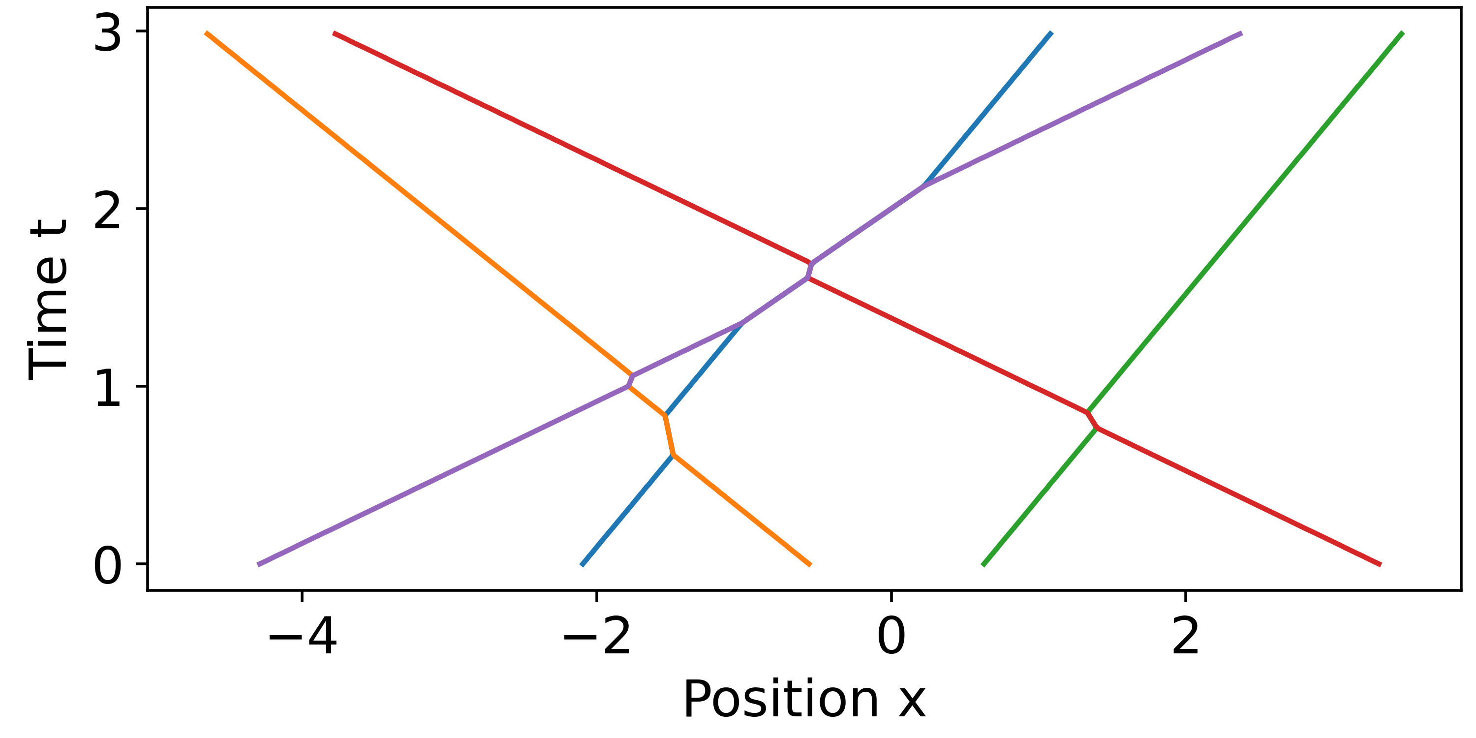
Figure 1: Sample of trajectories for the renormalised dynamics (13), given by (14), for the Lieb-Liniger model with $c=1$.

These trajectories are, of course, not an accurate description of the full many-body wave function $\Psi_{A_{t}}$: the results are valid in the large-deviation sense (and any small-scale regularisation will do). Paralleling thermodynamics, we are describing the “entropy density”, or large-deviation function, $I[\rho]$ associated to the amplitude modulation: with $\bar{\bm{x}},\,\bm{\theta}$ distributed as $\rho(\bar{x},\theta)$, we have $A\asymp e^{LI[\rho]}$, and under time evolution $I_{t}[\rho_{\bar{t}}]=I[\rho]$ where $\rho_{\bar{t}}(\bar{x},\theta)$ is induced by the trajectories (13) (recall $t=L\bar{t}$).

It is now a simple matter to argue that $\rho_{\bar{t}}(\bar{x},\theta)$ satisfies the GHD equation (1). The time derivative of (13) gives $\theta_{i}=\dot{x}_{i}+\sum_{j}\varphi(\theta_{ij})\delta(x_{ij})\dot{x}_{ij}$. With $\rho_{(\bm{x},\bm{\theta})}(\bar{x},\theta)=L^{-1}\sum_{i}\delta(\bar{x}-x_{i}/L)\delta(\theta-\theta_{i})$ the empirical density for $(\bm{x},\bm{\theta})$, we note, thanks to (2), that $\dot{x}_{i}=v^{\rm eff}_{\rho_{(\bm{x},\bm{\theta})}}(x_{i}/L,\theta_{i})$ is a solution. Using the exact continuity equation

$$\partial_{\bar{t}}\sum_{i}\delta(\bar{x}-\frac{x_{i}}{L})\delta(\theta-\theta_{i})+\partial_{\bar{x}}\sum_{i}\dot{x}_{i}\delta(\bar{x}-\frac{x_{i}}{L})\delta(\theta-\theta_{i})=0$$ (15)

we obtain (1) for the empirical density, and then for $\rho_{\bar{t}}(\bar{x},\theta)$ by taking the weak limit $\rho_{(\bm{x}_{t},\bm{\theta})}(\bar{x},\theta)\to\rho_{\bar{t}}(\bar{x},\theta)$.

Emergence of GHD in the quantum problem.— Let us write $\hat{\varrho}=e^{-\int{\rm d}x{\rm d}\theta\,\operatorname{He}\hat{\rho}[\beta]}$ in (7). Here we introduce the macroscopic $O(L)$ inhomogeneous charges is $\hat{\rho}[\beta]=\int{\rm d}x{\rm d}\theta\,\hat{\rho}(x,\theta)\beta(x,\theta)$, with $\beta(x,\theta)=\sum_{a}\beta_{a}(x)\theta^{a}=\bar{\beta}(x/L,\theta)$. A crucial observation is that these are essentially classical Goldstein et al. (2010): we can show using results of Doyon and Yoshimura (2017) that their commutators are $O(1)$, generalising the Poisson bracket found at that order for free fermions. In particular $e^{-\hat{\rho}[\beta]/2}|\Psi_{\bm{\theta}}\rangle=|\Psi_{A}\rangle$ where $A(\bm{x},\bm{\theta})\asymp e^{-\sum_{i}\beta(x_{i},\theta_{i})/2}$, and $\hat{\varrho}\asymp e^{-\hat{\rho}[\beta]^{\dagger}/2}e^{-\hat{\rho}[\beta]/2}$. See (SM, , Subsec 4.1).

Using these two relations, we obtain ${\rm Tr}\hat{\varrho}\asymp Z_{A}:=\sum_{N=0}^{\infty}\int_{{\mathbb{R}}^{N}_{>}}{\rm d}^{N}\theta\,||\Psi_{A}||^{2}.$ Writing out explicitly $||\Psi_{A}||^{2}$, $Z_{A}$ becomes a partition function for a signed measure $\mu$ on the many-particle phase space $(\bm{x},\bm{\theta})$ (see (SM, , Subsec 4.1)). By mean-field arguments, a local-density approximation (LDA) should hold, $Z_{A}\asymp e^{-L\int{\rm d}\bar{x}\,F[\bar{\beta}(\bar{x},\cdot)]}$ where $F$ is the specific free energy. The form of $F$ is not important here, but we give a full derivation at the Tonks-Girardeau point in (SM, , Subsec 4.2) (see also Granet (2023)).

The average (7) is then found by evolving forward, perturbing by a macroscopic source $\hat{\rho}[\gamma]$, $\gamma(x,\theta)=\bar{\gamma}(x/L,\theta)$, and evolving backward. From (12), this amounts to evaluating $Z_{A_{\gamma}}$, $A_{\gamma}(\bm{x},\bm{\theta})=A(\bm{x},\bm{\theta})e^{\sum_{i}\gamma(x_{t\,i},\theta_{i})/2}$:

$$\rho_{\rm p}(\theta,\bar{x},\bar{t})=\lim_{L\to\infty}L^{-1}\delta\log Z_{A_{\gamma}}/\delta\bar{\gamma}(\bar{x},\theta)|_{\gamma=0}$$ (16)

and we obtain $\rho_{\rm p}(\theta,\bar{x},\bar{t})=\mathbb{E}_{\mu}[\rho_{\bar{t}}(\bar{x},\theta)]$ (see (SM, , Subsec 4.1)). Here the $\bar{\gamma}(\bar{x},\theta)$-derivative gives a mesoscopic “fluid-cell” spatial mean of the empirical density $\rho_{(\bm{x}_{L\bar{t}},\bm{\theta})}(L\bar{x},\theta)$, as it is a response to a macroscopic perturbation; we may thus replace it by its weak limit $\rho_{\bar{t}}(\bar{x},\theta)$. It is now clear that the large-deviation form of the amplitude is sufficient to determine $\rho_{\rm p}(\theta,\bar{x},\bar{t})$: any dependence on $\bar{\gamma}$ in $A_{\gamma}$ that is less than $e^{O(L)}$ does not contribute upon taking $L^{-1}\delta/\delta\bar{\gamma}(\bar{x},\theta)$ in (16). Finally, by the LDA, $\rho_{\bar{t}=0}(\bar{x},\theta)$ is non-fluctuating: its $n^{\rm th}$ cumulant decays as $L^{1-n}$. As we have shown that $\rho_{\bar{t}}(\bar{x},\theta)$ satisfies the GHD equation, it is also non-fluctuating, and thus we have $\rho_{\rm p}(\theta,\bar{x},\bar{t})=\rho_{\bar{t}}(\bar{x},\theta)$, which therefore also satisfies the GHD equation. The deterministic evolution of fluid-cell means of conserved densities at the Euler scale was discussed in Doyon et al. (2022a, b); here we have argued for it from the large-deviation analysis of amplitude modulations.

Conclusion.— We have provided the first ab initio derivation of the equation of GHD in interacting quantum models, focusing on the Lieb-Liniger model. This, we believe, can serve as a blueprint for a rigorous proof, and the methods can be adapted to other Bethe-ansatz integrable models. Our derivation explains why the GHD equation has a simple classical interpretation in terms of gases of wave packets, connecting with semiclassical analysis (thus extending ideas from free fermion models Fagotti (2020)). A new family of integrable classical particle systems emerges, studied further in Doyon et al. . We believe the techniques can be used to obtain a deeper understanding of many large-scale effects, including external forces Doyon and Yoshimura (2017); Bastianello et al. (2019), correlation functions Doyon and Spohn (2017b); Doyon (2018); Fava et al. (2021); Nardis et al. (2022); Doyon et al. (2022a), quantum effects Ruggiero et al. (2020), macroscopic fluctuations Bertini et al. (2015); Doyon and Myers (2020); Myers et al. (2020); Doyon et al. (2022b), and diffusive and dispersive corrections De Nardis et al. (2018); Gopalakrishnan et al. (2018); Nardis et al. (2019); Durnin et al. (2021); Nardis and Doyon (2022); Ferrari and Olla (2023). In particular, this should help understand quantum macroscopic fluctuations Bernard (2021); Wienand et al. (2023). Our derivation suggests a route towards an extension of the semiclassical analysis Martinez (2002); Zworski (2012) to interacting wave packets.

Acknowledgments.— The authors are grateful to Alvise Bastianello, Thibault Bonnemain, Olalla Castro Alvaredo and Jacopo De Nardis for discussions. The work of BD was supported by the Engineering and Physical Sciences Research Council (EPSRC) under grant no EP/W010194/1. BD would like to thank the Isaac Newton Institute for Mathematical Sciences, Cambridge, for support and hospitality during the programmes “Dispersive hydrodynamics: mathematics, simulation and experiments, with applications in nonlinear waves” and “Building a bridge between non-equilibrium statistical physics and biology” where work on this paper was undertaken (EPSRC grant no EP/R014604/1). FH acknowledges funding from the faculty of Natural, Mathematical & Engineering Sciences at King’s College London.

References

- Abanov et al. (2021) A. Abanov, B. Doyon, J. Dubail, A. Kamenev, and H. Spohn, eds., Hydrodynamics of Low-Dimensional Quantum Systems (2021) special issue of J. Phys. A.
- Castro-Alvaredo et al. (2016) O. A. Castro-Alvaredo, B. Doyon, and T. Yoshimura, Phys. Rev. X 6, 041065 (2016).
- Bertini et al. (2016) B. Bertini, M. Collura, J. De Nardis, and M. Fagotti, Phys. Rev. Lett. 117, 207201 (2016).
- Zakharov (2009) V. E. Zakharov, Studies in Applied Mathematics 122, 219 (2009).
- El (2021) G. A. El, Journal of Statistical Mechanics: Theory and Experiment 2021, 114001 (2021).
- Suret et al. (2023) P. Suret, S. Randoux, A. Gelash, D. Agafontsev, B. Doyon, and G. El, “Soliton gas: Theory, numerics and experiments,” (2023), arXiv:2304.06541 [nlin.SI] .
- Doyon and Spohn (2017a) B. Doyon and H. Spohn, J. Stat. Mech. Theory Exp. 2017, 073210 (2017a).
- Cao et al. (2018) X. Cao, V. B. Bulchandani, and J. E. Moore, Phys. Rev. Lett. 120, 164101 (2018).
- Bastianello et al. (2018) A. Bastianello, B. Doyon, G. Watts, and T. Yoshimura, SciPost Phys. 4, 045 (2018).
- Spohn (2020) H. Spohn, J. Stat. Phys. 180, 4 (2020).
- Doyon (2019) B. Doyon, J. Math. Phys. 60, 073302 (2019).
- Bulchandani et al. (2019) V. B. Bulchandani, X. Cao, and J. E. Moore, Journal of Physics A: Mathematical and Theoretical 52, 33LT01 (2019).
- Koch and Bastianello (2023) R. Koch and A. Bastianello, “Exact thermodynamics and transport in the classical sine-gordon model,” (2023), arXiv:2303.16932 [cond-mat.stat-mech] .
- Doyon et al. (2017) B. Doyon, J. Dubail, R. Konik, and T. Yoshimura, Phys. Rev. Lett. 119, 195301 (2017).
- Bulchandani et al. (2017) V. B. Bulchandani, R. Vasseur, C. Karrasch, and J. E. Moore, Physical Review Letters 119 (2017), 10.1103/physrevlett.119.220604.
- Bulchandani et al. (2018) V. B. Bulchandani, R. Vasseur, C. Karrasch, and J. E. Moore, Phys. Rev. B 97, 045407 (2018).
- Caux et al. (2019) J.-S. Caux, B. Doyon, J. Dubail, R. Konik, and T. Yoshimura, SciPost Phys. 6, 070 (2019).
- Castro-Alvaredo et al. (2020) O. A. Castro-Alvaredo, C. De Fazio, B. Doyon, and F. Ravanini, Journal of High Energy Physics 2020, 45 (2020).
- Schemmer et al. (2019) M. Schemmer, I. Bouchoule, B. Doyon, and J. Dubail, Phys. Rev. Lett. 122, 090601 (2019).
- Malvania et al. (2021) N. Malvania, Y. Zhang, Y. Le, J. Dubail, M. Rigol, and D. S. Weiss, Science 373, 1129 (2021), https://www.science.org/doi/pdf/10.1126/science.abf0147 .
- Møller et al. (2021) F. Møller, C. Li, I. Mazets, H.-P. Stimming, T. Zhou, Z. Zhu, X. Chen, and J. Schmiedmayer, Phys. Rev. Lett. 126, 090602 (2021).
- Doyon (2020) B. Doyon, SciPost Phys. Lect. Notes , 18 (2020).
- Bastianello et al. (2022) A. Bastianello, B. Bertini, B. Doyon, and R. Vasseur, J. Stat. Mech. Theory Exp. 2022, 014001 (2022).
- Spohn (2023) H. Spohn, “Hydrodynamic scale of integrable many-particle systems,” (2023), arXiv:2301.08504 [cond-mat.stat-mech] .
- Essler (2022) F. H. Essler, Physica A: Statistical Mechanics and its Applications , 127572 (2022).
- Smirnov (1992) F. A. Smirnov, Form Factors in Completely Integrable Models of Quantum Field Theory (World Scientific, 1992).
- Mussardo (2010) G. Mussardo, Statistical field theory: an introduction to exactly solved models in statistical physics (Oxford University Press, 2010).
- Fagotti (2020) M. Fagotti, SciPost Phys. 8, 48 (2020).
- Granet (2023) E. Granet, “Wavelet representation of hardcore bosons,” (2023), arXiv:2303.17494 [cond-mat.quant-gas] .
- Calabrese et al. (2016) P. Calabrese, F. H. L. Essler, and G. Mussardo, Journal of Statistical Mechanics: Theory and Experiment 2016, 064001 (2016).
- Borsi et al. (2021) M. Borsi, B. Pozsgay, and L. Pristyák, J. Stat. Mech. Theory Exp. 2021, 094001 (2021).
- Cubero et al. (2021) A. C. Cubero, T. Yoshimura, and H. Spohn, J. Stat. Mech. Theory Exp. 2021, 114002 (2021).
- Boldrighini et al. (1983) C. Boldrighini, R. L. Dobrushin, and Y. M. Sukhov, J. Stat. Phys. 31, 577 (1983).
- Ferrari et al. (2022) P. A. Ferrari, C. Franceschini, D. G. E. Grevino, and H. Spohn, “Hard rod hydrodynamics and the levy chentsov field,” (2022), arXiv:2211.11117 [math.PR] .
- Ferrari et al. (2021) P. A. Ferrari, C. Nguyen, L. T. Rolla, and M. Wang, Forum of Mathematics, Sigma 9, e60 (2021).
- Croydon and Sasada (2020) D. A. Croydon and M. Sasada, Commun. Math. Phys. 383, 427 (2020).
- El (2003) G. El, Physics Letters A 311, 374 (2003).
- El and Tovbis (2020) G. El and A. Tovbis, Physical Review E 101, 052207 (2020).
- Faddeev (1996) L. D. Faddeev, “How algebraic Bethe ansatz works for integrable model,” (1996), arXiv:hep-th/9605187 [hep.th] .
- Lieb and Liniger (1963) E. H. Lieb and W. Liniger, Phys. Rev. 130, 1605 (1963).
- Bouchoule and Dubail (2022) I. Bouchoule and J. Dubail, Journal of Statistical Mechanics: Theory and Experiment 2022, 014003 (2022).
- Mistakidis et al. (2022) S. Mistakidis, A. Volosniev, R. Barfknecht, T. Fogarty, T. Busch, A. Foerster, P. Schmelcher, and N. Zinner, “Cold atoms in low dimensions – a laboratory for quantum dynamics,” (2022), arXiv:2202.11071 [cond-mat.quant-gas] .
- Grava (2016) T. Grava, “Whitham modulation equations and application to small dispersion asymptotics and long time asymptotics of nonlinear dispersive equations,” in Rogue and Shock Waves in Nonlinear Dispersive Media, edited by M. Onorato, S. Resitori, and F. Baronio (Springer International Publishing, Cham, 2016) pp. 309–335.
- Spohn (2012) H. Spohn, Large scale dynamics of interacting particles (Springer Science & Business Media, 2012).
- Zamolodchikov and Zamolodchikov (1979) A. B. Zamolodchikov and A. B. Zamolodchikov, Annals of Physics 120, 253 (1979).
- Novikov et al. (1984) S. Novikov, S. Manakov, L. Pitaevskii, and V. E. Zakharov, Theory of solitons: the inverse scattering method (Springer Science & Business Media, 1984).
- Faddeev and Takhtajan (1987) L. D. Faddeev and L. A. Takhtajan, Hamltonian methods in the theory of solitons (1987).
- El and Kamchatnov (2005) G. A. El and A. M. Kamchatnov, Phys. Rev. Lett. 95, 204101 (2005).
- Doyon et al. (2018a) B. Doyon, T. Yoshimura, and J.-S. Caux, Phys. Rev. Lett. 120, 045301 (2018a).
- Bonnes et al. (2014) L. Bonnes, F. H. L. Essler, and A. M. Läuchli, Phys. Rev. Lett. 113, 187203 (2014).
- (51) B. Doyon, F. Hübner, and T. Yoshimura, “-deformations of classical free particles,” To appear.
- Gaudin (2014) M. Gaudin, The Bethe wavefunction (Cambridge University Press, 2014).
- (53) See the Supplemental Material.
- Yang and Yang (1969) C. N. Yang and C. P. Yang, Journal of Mathematical Physics 10, 1115 (1969), https://pubs.aip.org/aip/jmp/article-pdf/10/7/1115/8144272/1115_1_online.pdf .
- Mossel and Caux (2012) J. Mossel and J.-S. Caux, Journal of Physics A: Mathematical and Theoretical 45, 255001 (2012).
- Davies (1990) B. Davies, Physica A: Statistical Mechanics and its Applications 167, 433 (1990).
- Davies and Korepin (2011) B. Davies and V. E. Korepin, “Higher conservation laws for the quantum non-linear schroedinger equation,” (2011), arXiv:1109.6604 [math-ph] .
- Ilievski et al. (2016) E. Ilievski, E. Quinn, J. D. Nardis, and M. Brockmann, Journal of Statistical Mechanics: Theory and Experiment 2016, 063101 (2016).
- Rudin (1991) W. Rudin, Functional analysis (McGraw-Hill, 1991).
- Cardy and Doyon (2022) J. Cardy and B. Doyon, Journal of High Energy Physics 2022, 136 (2022).
- Doyon et al. (2018b) B. Doyon, H. Spohn, and T. Yoshimura, Nucl. Phys. B 926, 570 (2018b).
- Goldstein et al. (2010) S. Goldstein, J. L. Lebowitz, R. Tumulka, and N. Zanghi, Eur. Phys. J. H 35, 173 (2010).
- Doyon and Yoshimura (2017) B. Doyon and T. Yoshimura, SciPost Phys. 2, 014 (2017).
- Doyon et al. (2022a) B. Doyon, G. Perfetto, T. Sasamoto, and T. Yoshimura, “Emergence of hydrodynamic spatial long-range correlations in nonequilibrium many-body systems,” (2022a), arXiv:2210.10009 [cond-mat.stat-mech] .
- Doyon et al. (2022b) B. Doyon, G. Perfetto, T. Sasamoto, and T. Yoshimura, “Ballistic macroscopic fluctuation theory,” (2022b), arXiv:2206.14167 [cond-mat.stat-mech] .
- Bastianello et al. (2019) A. Bastianello, V. Alba, and J.-S. Caux, Phys. Rev. Lett. 123, 130602 (2019).
- Doyon and Spohn (2017b) B. Doyon and H. Spohn, SciPost Phys. 3, 039 (2017b).
- Doyon (2018) B. Doyon, SciPost Phys. 5, 054 (2018).
- Fava et al. (2021) M. Fava, S. Biswas, S. Gopalakrishnan, R. Vasseur, and S. Parameswaran, PNAS 118, e2106945118 (2021).
- Nardis et al. (2022) J. D. Nardis, B. Doyon, M. Medenjak, and M. Panfil, Journal of Statistical Mechanics: Theory and Experiment 2022, 014002 (2022).
- Ruggiero et al. (2020) P. Ruggiero, P. Calabrese, B. Doyon, and J. Dubail, Phys. Rev. Lett. 124, 140603 (2020).
- Bertini et al. (2015) L. Bertini, A. De Sole, D. Gabrielli, G. Jona-Lasinio, and C. Landim, Rev. Mod. Phys. 87, 593 (2015).
- Doyon and Myers (2020) B. Doyon and J. Myers, Annales Henri Poincaré 21, 255 (2020).
- Myers et al. (2020) J. Myers, M. J. Bhaseen, R. J. Harris, and B. Doyon, SciPost Phys. 8, 007 (2020).
- De Nardis et al. (2018) J. De Nardis, D. Bernard, and B. Doyon, Phys. Rev. Lett. 121, 160603 (2018).
- Gopalakrishnan et al. (2018) S. Gopalakrishnan, D. A. Huse, V. Khemani, and R. Vasseur, Phys. Rev. B 98, 220303(R) (2018).
- Nardis et al. (2019) J. D. Nardis, D. Bernard, and B. Doyon, SciPost Phys. 6, 049 (2019).
- Durnin et al. (2021) J. Durnin, A. D. Luca, J. D. Nardis, and B. Doyon, Journal of Physics A: Mathematical and Theoretical 54, 494001 (2021).
- Nardis and Doyon (2022) J. D. Nardis and B. Doyon, “Hydrodynamic gauge fixing and higher order hydrodynamic expansion,” (2022), arXiv:2211.16555 [cond-mat.stat-mech] .
- Ferrari and Olla (2023) P. A. Ferrari and S. Olla, “Macroscopic diffusive fluctuations for generalized hard rods dynamics,” (2023), arXiv:2305.13037 [math-ph] .
- Bernard (2021) D. Bernard, Journal of Physics A: Mathematical and Theoretical 54, 433001 (2021).
- Wienand et al. (2023) J. F. Wienand et al., “Emergence of fluctuating hydrodynamics in chaotic quantum systems,” (2023), arXiv:2306.11457 [cond-mat.quant-gas] .
- Martinez (2002) A. Martinez, An Introduction to Semiclassical and Microlocal Analysis, Universitext (Springer New York, 2002).
- Zworski (2012) M. Zworski, Semiclassical Analysis, Graduate Studies in Mathematics, Vol. 138 (American Mathematical Society, 2012).