Model-free selective inference under covariate shift
via weighted conformal p-values

Abstract

This paper introduces novel weighted conformal p-values and methods for model-free selective inference. The problem is as follows: given test units with covariates $X$ and missing responses $Y$, how do we select units for which the responses $Y$ are larger than user-specified values while controlling the proportion of false positives? Can we achieve this without any modeling assumptions on the data and without any restriction on the model for predicting the responses? Last, methods should be applicable when there is a covariate shift between training and test data, which commonly occurs in practice.

We answer these questions by first leveraging any prediction model to produce a class of well-calibrated weighted conformal p-values, which control the type-I error in detecting a large response. These p-values cannot be passed onto classical multiple testing procedures since they may not obey a well-known positive dependence property. Hence, we introduce weighted conformalized selection (WCS), a new procedure which controls false discovery rate (FDR) in finite samples. Besides prediction-assisted candidate selection, WCS (1) allows to infer multiple individual treatment effects, and (2) extends to outlier detection with inlier distributions shifts. We demonstrate performance via simulations and applications to causal inference, drug discovery, and outlier detection datasets.

1 Introduction

Many scientific discovery and decision making tasks concern the selection of promising candidates from a potentially large pool. In drug discovery, scientists aim to find drug candidates—from a huge chemical space of molecules or compounds—with sufficiently high binding affinity to a target. College admission officers or hiring managers seek applicants with a high potential of excellence. In healthcare, one would like to allocate resources to individuals who would benefit the most. The list of such examples is endless. In all these problems, a decision maker would like to identify those units for which an unknown outcome of interest (affinity for a target molecule/job performance/reduction in stress level) takes on a large value.

Machine learning has shown tremendous potential for accelerating these resource- and time-consuming processes whereby predictions for the unknown outcomes are used to shortlist promising candidates before any further in-depth investigation [LDG13, CH18, SSKMM19]. This is a sharp departure from traditional strategies that either directly evaluate the outcomes via a physical screening to determine drug binding affinities, or “predict” the unknown outcomes via human judgement in healthcare or job hiring applications. In the new paradigm, a prediction model draws evidence from training data to inform values the unknown outcome may take on given the features of a unit.

If the intent is thus to use machine learning to screen candidates, we would need to understand and control the uncertainty in black-box prediction models as a selection tool. First, gathering evidence for new discoveries from past instances is challenging as they are not necessarily similar; i.e. they may be drawn from distinct distributions. Second, since a subsequent investigation applied to the shortlisted candidates is often resource intensive, it is meaningful to limit the error rate on the selected. It is not so much the accuracy of the prediction that matters, rather the proportion of selected units not passing the test. Keeping such a proportion at sufficiently low levels is a non-traditional criterion in typical prediction problems.

This paper studies the reliable selection of promising units/individuals whose unknown outcomes are sufficiently large. We develop methods that apply in a model-free fashion—without making any modeling assumptions on the data generating process while controlling the expected proportion of false discoveries among the selected.

1.1 Reliable selection under distribution shift

Formally, suppose test samples $\{(X_{j},Y_{j})\}_{j\in\mathcal{D}_{\textnormal{test}}}$ are drawn i.i.d. from an unknown distribution $Q$, whose outcomes $\{Y_{j}\}_{j\in\mathcal{D}_{\textnormal{test}}}$ are unobserved. Our goal is to identify a subset $\mathcal{R}\subseteq\mathcal{D}_{\textnormal{test}}$ with outcomes above some known, potentially random, thresholds $\{c_{j}\}_{j\in\mathcal{D}_{\textnormal{test}}}$. To draw statistical evidence for large outcomes in $\mathcal{D}_{\textnormal{test}}$, we assume we hold an independent set of i.i.d. calibration data $\{(X_{i},Y_{i})\}_{i\in\mathcal{D}_{\textnormal{calib}}}$ whose outcomes are, this time, observed.

Before we begin our discussion, we note that a challenge that underlies almost all applications is that samples in $\mathcal{D}_{\textnormal{calib}}$ are often different from those in $\mathcal{D}_{\textnormal{test}}$. That is, in many cases, a point $(X_{j},Y_{j})$ in $\mathcal{D}_{\textnormal{test}}$ is sampled from $Q$ while a point $(X_{i},Y_{i})$ in $\mathcal{D}_{\textnormal{calib}}$ is sampled from a different distribution $P$. We elaborate on the distribution shift issue by considering two motivating examples.

Drug discovery.

Virtual screening, which identifies viable drug candidates using predicted affinity scores from supervised machine learning models, is increasingly popular in early stages of drug discovery [Hua07, KMLH17, VCC⁺19, DDJ⁺21]. In this application, $\mathcal{D}_{\textnormal{calib}}$ is the set of drugs with known affinities, while $\mathcal{D}_{\textnormal{test}}$ is the set of new drugs whose binding affinities are of interest. In practice, there usually is a distribution shift between the two batches: for instance, an experimenter may favor a specific structure when choosing candidates to physically screen their true binding affinities [PPS⁺15]. Since physically screened drugs are subsequently added to the calibration dataset $\mathcal{D}_{\textnormal{calib}}$, they may not be representative of the new drugs in $\mathcal{D}_{\textnormal{test}}$. Accounting for such distribution shifts when applying virtual screening is crucial for the reliability of the whole drug discovery process, and has attracted recent attention [Krs21].

College admission.

A college may be interested in prospective students who are likely to graduate after four years of undergraduate education (a binary outcome of interest) among all applicants in $\mathcal{D}_{\textnormal{test}}$ as to maintain a reasonable graduation rate. The issue is that $\mathcal{D}_{\textnormal{calib}}$ usually consists of students who were admitted in the past as the outcome is only known for these students. Since previous cohorts may have been selected by applying various admission criteria, the distribution of the training data is different from that of the new applicants even if the distribution of applicants does not much vary over the years. Similar concerns apply to job hiring when using prediction models to select suitable applicants [FRTT12, SS16]; the way an institution chooses to record the outcomes of former candidates can lead to a discrepancy between the documented candidates and those under consideration.

In this paper, we propose to address the distribution shift issue by considering a scenario where the shift can be entirely attributed to observed covariates; this is commonly referred to as a covariate shift in the literature [SKM07, TFBCR19]. Concretely, we assume that there is some function $w\colon\mathcal{X}\to\mathbb{R}^{+}$ such that

$$\frac{{\,\mathrm{d}}Q}{{\,\mathrm{d}}P}(x,y)=w(x),\quad P\textrm{-almost surely},$$ (1)

where ${\,\mathrm{d}}Q/{\,\mathrm{d}}P$ denotes the Radon-Nikodym derivative. While all kinds of distribution shift could happen in practice, covariate shift—widely used to characterize distribution shifts caused by selection on known features—covers many important cases. In drug discovery, if the preference for choosing which samples to screen only depends upon the covariates, e.g. the sequence of amino acids of the compound or the physical properties of the compound, we are dealing with the covariate shift (1). In college admission or job hiring, if a specific type of applicant—characterized by certain features—were favored in previous admission/hiring cycles, such a preference would yield the shift (1) between previous students/employees and current applicants.

Returning to our decision problem, we are interested in finding as many units $j\in\mathcal{D}_{\textnormal{test}}$ as possible with $Y_{j}>c_{j}$, while controlling the false discovery rate (FDR) below some pre-specified level $q\in(0,1)$. The FDR is the expected fraction of false discoveries, where a false discovery is a selected unit for which $Y_{j}\leq c_{j}$, i.e., the outcome turns out to fall below the threshold. Formally, we wish to find $\mathcal{R}$ obeying

$$\textnormal{FDR}:=\mathbb{E}\Bigg{[}\frac{\sum_{j\in\mathcal{D}_{\textnormal{test}}}\operatorname{\mathds{1}}\{j\in\mathcal{R},Y_{j}\leq c_{j}\}}{\max\{1,|\mathcal{R}|\}}\Bigg{]}\leq q,$$ (2)

where $q$ is the nominal target FDR level. The expectation in (2) is taken over both the new test samples and the calibration data/screening procedure. The FDR quantifies the tradeoff between resources dedicated to the shortlisted candidates and the benefits from true positives [BH95]. By controlling the FDR, we ensure that a sufficiently large proportion of follow-up resources—such as clinical trials in drug discovery, human evaluation of student profiles and interviews—to confirm predictions from machine learning models are devoted to interesting candidates.

The problem of FDR-controlled selection with machine learning predictions has been studied in an earlier paper [JC22] under the assumption of no distribution shift. This means the new instances are exchangeable with the known calibration data, which, as we discussed above, is rarely the case in practice. Therefore, there is a pressing need for novel techniques to address the distribution shift issue.

1.2 Preview of theoretical contributions

Our strategy consists in (1) constructing a calibrated confidence measure (p-value), which applies to any predictive model, for detecting a large unknown outcome, and (2) in employing multiple testing ideas to build the selection set from test p-values.

Weighted conformal p-value: a calibrated confidence measure.

We introduce random variables $\{p_{j}\}_{j\in\mathcal{D}_{\textnormal{test}}}$, which resemble p-values in the sense that for each $j\in\mathcal{D}_{\textnormal{test}}$, they obey

$$\mathbb{P}(p_{j}\leq t,~{}Y_{j}\leq c_{j})\leq t,\quad\textrm{for all}~{}t\in[0,1],$$ (3)

where the probability is over both the calibration data and the test sample $(X_{j},Y_{j},c_{j})$. This is similar to the definition of a classical p-value, hence, we call $p_{j}$ a“p-value”. With this, for any $\alpha\in(0,1)$, selecting $j$ if and only if $p_{j}\leq\alpha$ controls the type-I error below $\alpha$ (the chance that $Y_{j}$ is below threshold is at most $\alpha$). Note however that (3) is perhaps an unconventional notion of type-I error, since it accounts for the randomness in the “null hypothesis” $H_{j}\colon Y_{j}\leq c_{j}$.

We construct $p_{j}$ using ideas from conformal prediction [VGS05, TFBCR19]. Take any monotone function $V\colon\mathcal{X}\times\mathcal{Y}\to\mathbb{R}$ (see Definition 2.1) built upon any prediction model that is independent of $\mathcal{D}_{\textnormal{calib}}$ and $\mathcal{D}_{\textnormal{test}}$. A concrete instance is $V(x,y)=y-\widehat{\mu}(x)$, where $\widehat{\mu}\colon\mathcal{X}\to\mathcal{Y}$ is any predictor trained on a held-out dataset. With scores $V_{i}=V(X_{i},Y_{i})$, $i\in\mathcal{D}_{\textnormal{calib}}$, and weight function $w(\cdot)$ given by (1), we construct $p_{j}$ to be approximately equal to $\widehat{F}(\widehat{V}_{j})$, where $\widehat{F}(\cdot)$ is the cumulative distribution function (c.d.f.) of the empirical distribution

$$\frac{\sum_{i\in\mathcal{D}_{\textnormal{calib}}}\,w(X_{i})\,\delta_{V_{i}}}{\sum_{i\in\mathcal{D}_{\textnormal{calib}}}w(X_{i})}.$$

While the precise definition of $p_{j}$ is in Section 2, Figure 1 visualizes the idea.

Intuitively, $p_{j}$ contrasts the value of $\widehat{V}_{j}=V(X_{j},c_{j})$ against the distribution of the unknown ‘oracle’ score $V_{j}=V(X_{j},Y_{j})$. The latter is approximated by $\widehat{F}(\cdot)$, which reweights the training data with weights reflecting the covariate shift (1). As such, $\widehat{F}(V_{j})$ is approximately uniformly distributed in $[0,1]$. Thus, a notably small value of $p_{j}\approx\widehat{F}(\widehat{V}_{j})$ relative to the uniform distribution informs that $\widehat{V}_{j}$ is smaller than what is typical of $V_{j}$, which further suggests evidence for $Y_{j}\geq c_{j}$. Leveraging conformal prediction techniques, such high-level ideas are made exact to achieve (3).

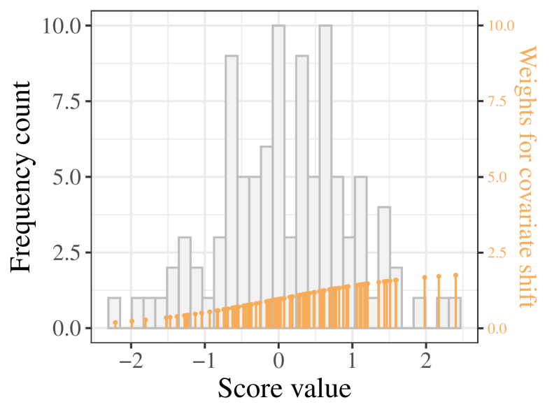
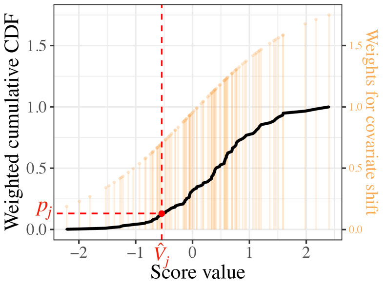
Figure 1: Visualization of weighted conformal p-values. Left: Distribution of scores in the calibration set (gray) and individual values of $w(X_{i})$ (orange) for $i\in\mathcal{D}_{\textnormal{calib}}$. Right: Weighted empirical c.d.f. of $\{V_{i}\}_{i\in\mathcal{D}_{\textnormal{calib}}}$; the red dashed lines illustrate how $p_{j}$ is computed from $\widehat{V}_{j}$, in which $j\in\mathcal{D}_{\textnormal{test}}$.

Intricate dependence among weighted conformal p-values.

Going beyond per-unit type-I error control, selecting from multiple test samples requires dealing with multiple p-values $\{p_{j}\}_{j\in\mathcal{D}_{\textnormal{test}}}$. A natural idea is then to use multiple testing ideas as if $\{p_{j}\}$ were classical p-values. However, the situation is complicated here because $\{p_{j}\}_{j\in\mathcal{D}_{\textnormal{test}}}$ all depend on the same set of calibration data, and, in sharp contrast to classical multiple testing, there is another source of randomness in the unknown outcomes.

Our second theoretical result shows the mutual dependence among multiple p-values is particularly challenging. It states that the favorable positive dependence structure among p-values, which was the key to FDR control with other p-values derived with conformal prediction ideas [BCL⁺21, JC22], can be violated in the presence of data-dependent weights in (4). As a result, it remains unclear whether applying existing multiple testing procedures controls the FDR in finite samples.

Weighted Conformalized Selection (WCS).

Last, we introduce WCS, a new procedure that achieves finite-sample FDR control under distribution shift. The idea is to calibrate the selection threshold for each $j\in\mathcal{D}_{\textnormal{test}}$ using a set of “auxiliary” p-values $\{\bar{p}_{\ell}^{(j)}\}_{\ell\in\mathcal{D}_{\textnormal{test}}}$. These p-values happen to obey a special conditional independence property, namely,

$$\bar{p}_{j}^{(j)}\perp\!\!\!\perp\{\bar{p}_{\ell}^{(j)}\}_{\ell\neq j}\,\big{|}\,\mathcal{Z}_{j},$$

where $\mathcal{Z}_{j}$ is the unordered set of the calibration data and the $j$-th test sample. We show that FDR control is valid regardless of the machine learning model used in constructing $V(\cdot,\cdot)$, and applies to a wide range of scenarios where the cutoffs $c_{j}$ can themselves be random variables.

1.3 Broader scope

Our methods happen to be applicable to additional statistical inference problems.

Multiple counterfactual inference.

The individual treatment effect (ITE) is a random variable that characterizes the difference between an individual’s outcome when receiving a treatment versus not, whose inference relies on comparing the observed outcome with the counterfactual [IR15, LC21, JRC23]. To infer the counterfactual of a unit under treatment, the calibration data are units who do not receive the treatment. If the treatment assignment depends on the covariates, then there may be, and usually will be, a covariate shift between treated and control units. We discuss this problem in Section 5.

Outlier detection.

Imagine we have access to i.i.d. inliers $\{Z_{i}\}_{i\in\mathcal{D}_{\textnormal{calib}}}$ from an unknown distribution $P$. Then outlier detection [BCL⁺21] seeks to find outliers among new samples $\{Z_{j}\}_{j\in\mathcal{D}_{\textnormal{test}}}$, i.e., those which do not follow the inlier distribution $P$. A potential application is fraud detection in financial transactions, where controlling the FDR ensures reasonable resource allocation in follow-up inquiries. However, financial behavior varies with users and it is possible that normal transactions of interest follow different distributions across different populations. A related problem is to detect concept drifts; that is, allowing a subset of features $X\subseteq Z$ to follow a distinct distribution, and only detecting test samples whose $Z{\,|\,}X$ distribution differs from $P_{Z{\,|\,}X}$. We discuss this problem in Section 6.

As in (3), the FDR (2) is marginalized over the randomness in the hypotheses. To this end, WCS requires all $\{X_{n+j},Y_{n+j}\}_{j=1}^{m}$ to be i.i.d. draws from a super-population. To relax this, we generalize our methods to control a notion of FDR that is conditional on the random hypotheses. This is useful for handling imbalanced data in classification, and the aforementioned outlier detection problem.

1.4 Data and code

An R package, ConfSelect, that implements Weighted Conformalized Selection (as well as the version without weights) together with code to reproduce all experiments in this paper, can be found in the GitHub repository https://github.com/ying531/conformal-selection.

1.5 Related work

Our methods build upon the conformal inference framework [VGS05] to infer unknown outcomes. There, the theoretical guarantee for conformal prediction sets is usually marginally valid over the randomness in a single test point. As discussed in [JC22], one might be interested in multiple test samples simultaneously; in such situations, standard conformal prediction tools are insufficient.

This work is connected to a recent line of research on selective inference issues arising in predictive inference. Some works use conformal p-values (whose definition differs from ours) with ‘full’ observations $\{(X_{j},Y_{j})\}_{j\in\mathcal{D}_{\textnormal{test}}}$—that is, the response is observed—for outlier detection, i.e., for identifying whether $(X_{j},Y_{j})$ follows the same distribution as the calibration data $\{(X_{i},Y_{i})\}_{i\in\mathcal{D}_{\textnormal{calib}}}$ [BCL⁺21, LSS22, MLMR22]. Whereas these methods do not consider distribution shift between calibration and test inliers, Section 6 extends all this. Here, the response $Y_{n+j}$—the object of inference—is not observed and, therefore, the problem is completely different. Consequently, methods and techniques to deal with this are new. Our focus on FDR control is similar in spirit to other recent papers; for instance, rather than marginal coverage of prediction sets, [FSJB22] studies the number of false positives, and [BHRZ23] the miscoverage rate on selected units.

Our methodology draws ideas from the multiple hypothesis testing literature, where the FDR is a popular type-I error criterion in exploratory analysis for controlling the proportion of ‘false leads’ in follow-up studies [BH95, BY01]. This paper is distinct from the conventional setting. First, testing a random outcome instead of a model parameter leads to a random null set and a complicated dependence structure. Second, our inference relies on (weighted) exchangeability of the data while imposing no assumptions on their distributions. In contrast, a null hypothesis often specifies the distribution of test statistics or p-values. Later on, we shall also draw connections to a recent literature dealing with dependence in multiple testing, such as that concerned with e-values [VW21, WR20] and conditional calibration of the BH procedure [FL22].

The application of our method is related to a substantial literature that emphasizes the importance of uncertainty quantification in drug discovery [NCBE14, SNB17, AHBC17, SAN⁺18, CCB19, WJR22]. Although existing works aim to employ conformal inference to assign confidence to machine prediction, this is often done in heuristic ways, which potentially invalidates the guarantees of conformal prediction due to selection issues. Instead, we provide here a principled approach to prioritizing drug candidates with clear and interpretable error control (i.e., guaranteeing a sufficiently high ‘hit rate’ [WJR22]), and offer a potential solution to the widely recognized distribution shift problem [Krs21, FL23].

The application to individual treatment effects in Section 5 is connected to [CDLM21]; the distinction is that they focus on a summary statistic such as a population quantile of the ITEs, while our method detects individuals with positive ITEs. Also related is [DWR21], which tests individuals for positive treatment effects with FDR control; however, in their setting a positive ITE means the whole distribution of the control outcome is dominated by that of the treated outcome, whereas we directly compare two random variables. Accordingly, our techniques are very different from these two references.

2 Weighted conformal p-values

2.1 Construction of weighted conformal p-values

Our weighted conformal p-values build upon any monotone score function, defined as follows.

Definition 2.1 (Monotonicity).

A score function $V(\cdot,\cdot)\colon\mathcal{X}\times\mathcal{Y}\to\mathbb{R}$ is monotone if $V(x,y)\leq V(x,y^{\prime})$ holds for any $x\in\mathcal{X}$ and any $y,y^{\prime}\in\mathcal{Y}$ obeying $y\leq y^{\prime}$.

Intuitively, the score function (often referred to as nonconformity score in conformal prediction [VGS05]) describes how well a hypothesized value $y\in\mathcal{Y}$ conforms to the machine prediction. A popular and monotone nonconformity score is $V(x,y)=y-\widehat{\mu}(x)$, where $\widehat{\mu}\colon\mathcal{X}\to\mathbb{R}$ is a point prediction; other choices include those based on quantile regression [RPC19] or estimates of the conditional c.d.f. [CWZ21].

From now on, write $\mathcal{D}_{\textnormal{calib}}=\{1,\dots,n\}$ and $\mathcal{D}_{\textnormal{test}}=\{n+1,\dots,n+m\}$. Compute $V_{i}=V(X_{i},Y_{i})$ for $i=1,\dots,n$ and $\widehat{V}_{n+j}=V(X_{n+j},c_{n+j})$ for $j=1,\dots,m$. Our weighted conformal p-values are defined as

$$p_{j}=\frac{\sum_{i=1}^{n}w(X_{i})\operatorname{\mathds{1}}{\{V_{i}<\widehat{V}_{n+j}\}}+(w(X_{n+j})+\sum_{i=1}^{n}w(X_{i})\operatorname{\mathds{1}}{\{V_{i}=\widehat{V}_{n+j}\}})\cdot U_{j}}{\sum_{i=1}^{n}w(X_{i})+w(X_{n+j})},$$ (4)

where $w(\cdot)$ is the covariate shift function in (1), and $U_{j}\stackrel{{\scriptstyle\textnormal{i.i.d.}}}{{\sim}}\textrm{Unif}([0,1])$ are tie-breaking random variables. When $w(\cdot)\equiv 1$, our p-values reduce to the conformal p-values in [JC22], see Appendix A.1. We also refer readers to Appendix A.2 for the connection between our p-values and conformal prediction intervals.

Roughly speaking, with a monotone score, the p-value (4) measures how small $c_{n+j}$ is compared with typical values of $Y_{n+j}$, and provides calibrated evidence for a large outcome as expressed in (3). This can be derived using conformal inference theory [TFBCR19] and the monotocity of $V$. We include a formal result here for completeness, whose proof is in Appendix B.1.

Lemma 2.2.

The tail inequality (3) holds if the covariate shift (1) holds and the score function is monotone.

Consequently, selecting a unit if $p_{j}\leq\alpha$ controls the type-I error at level $\alpha$ for each $j\in\mathcal{D}_{\textnormal{test}}$. We shall however see that dealing with multiple test samples is far more challenging.

2.2 Weighted conformal p-values are not PRDS

Applying multiple testing procedures to our p-values to obtain a selection set naturally comes to mind. Previous works applying the Benjamini-Hochberg (BH) procedure [BH95] to p-values obtained via conformal inference ideas indeed control the FDR [BCL⁺21, JC22, MLMR22]. This is because the p-values obey a favorable dependence structure called positive dependence on a subset (PRDS).

Definition 2.3 (PRDS).

A random vector $X=(X_{1},\dots,X_{m})$ is PRDS on a subset $\mathcal{I}$ if for any $i\in\mathcal{I}$ and any increasing set $D$, the probability $\mathbb{P}(X\in D{\,|\,}X_{i}=x)$ is increasing in $x$.

Above, a set $D\subseteq\mathbb{R}^{m}$ is increasing if $a\in D$ and $b\succeq a$ implies $b\in D$ ($b\succeq a$ means that all the components of $b$ are larger than or equal to those of $a$). It is well-known that the BH procedure controls the FDR when applied to PRDS p-values [BY01]. The PRDS property among (unweighted) conformal p-values was first studied in [BCL⁺21], and generalized in [JC22] to plug-in values $c_{n+j}$ in lieu of $Y_{n+j}$, thereby forming the basis for FDR control. If the PRDS property were to hold for the weighted conformal p-values, then applying the BH procedure would also control the FDR. This is however not always the case; a constructive proof of Proposition 2.4 is in Appendix B.3.

Proposition 2.4.

There exist a sample size $n$, a weight function $w\colon\mathcal{X}\to\mathbb{R}^{+}$, a nonconformity score $V\colon\mathcal{X}\times\mathcal{Y}\to\mathbb{R}$, and distributions $P$ and $Q$ obeying (1), such that the weighted conformal p-values (4) are not PRDS for $\{X_{i},Y_{i}\}_{i=1}^{n}\stackrel{{\scriptstyle\textnormal{i.i.d.}}}{{\sim}}P$ and $\{X_{n+j},Y_{n+j}\}_{j=1}^{m}\stackrel{{\scriptstyle\textnormal{i.i.d.}}}{{\sim}}Q$.

A little more concretely, we find that the PRDS property is likely to fail when the nonconformity scores are negatively correlated with the weights. Note that the dependence among conformal p-values arises from sharing the calibration data. Under exchangeability (i.e. taking equal weightes $w(x)\equiv 1$), a smaller conformal p-value is (only) associated with larger calibration scores, and hence smaller p-values for other test points. However, with negatively associated weights and scores, a smaller p-value may also be due to smaller calibration weights—instead of larger calibration scores—which implies that other p-values may take on larger values.

2.3 BH procedure controls FDR asymptotically

Before introducing our new selection methods, we nevertheless show asymptotic FDR control using the BH procedure.

Theorem 2.5.

Suppose $w(\cdot)$ is uniformly bounded by a fixed constant, the covariate shift (1) holds, and $\{c_{n+j}\}_{j=1}^{m}$ are i.i.d. random variables. Fix any $q\in(0,1)$, and let $\mathcal{R}$ be the output of the BH procedure applied to $\{p_{j}\}_{j=1}^{m}$ in (4). Then the following results hold.

1. For any fixed $m$, it holds that $\limsup_{n\to\infty}\textnormal{FDR}\leq q$.

2. Suppose $m,n\to\infty$. Under a mild technical condition (see Appendix A.4), $\limsup_{m,n\to\infty}\textnormal{FDR}\leq q$. Furthermore, the asymptotic FDR and power of BH can be exactly characterized in this case.

We provide the complete technical version of Theorem 2.5 in Theorem A.3, whose proof is in Appendix B.4. In fact, we prove that as $n\to\infty$, the weighted conformal p-values converge to i.i.d. random variables that are dominated by the uniform distribution, which ensures asymptotic FDR control (see Appendix B.4 for details). The technical condition we impose resembles that in [STS04], which ensures the existence of a limit point of the rejection threshold and enables the asymptotic analysis.

We also remark that the PRDS property is a sufficient, but not necessary, condition for the BH procedure to control the FDR. In fact, we will see that the BH procedure with weighted conformal p-values empirically controls the FDR in all of our numerical experiments, hence it remains a reasonable option in practice.

3 Finite-sample FDR control

We now introduce a new multiple testing procedure, WCS, that controls the FDR in finite samples with weighted conformal p-values. Our method builds on the following p-values:

$${p}_{j}=\frac{\sum_{i=1}^{n}w(X_{i})\operatorname{\mathds{1}}{\{V_{i}<\widehat{V}_{n+j}\}}+w(X_{n+j})}{\sum_{i=1}^{n}w(X_{i})+w(X_{n+j})}.$$ (5)

It is a slight modification of (4) up to random tie-breaking. The asymptotic results in Theorem 2.5 also hold with these p-values as long as the distributions of the $V_{i}$’s and $\widehat{V}_{n+j}$’s do not have point masses.

3.1 Weighted Conformalized Selection

As before, we compute $V_{i}=V(X_{i},Y_{i})$ for $i=1,\dots,n$ and $\widehat{V}_{n+j}=V(X_{n+j},c_{n+j})$ for $j=1,\dots,m$. For each $j$, we compute a set of auxiliary p-values

$${p}_{\ell}^{(j)}:=\frac{\sum_{i=1}^{n}w(X_{i})\operatorname{\mathds{1}}{\{V_{i}<\widehat{V}_{n+\ell}\}}+w(X_{n+j})\operatorname{\mathds{1}}{\{\widehat{V}_{n+j}<\widehat{V}_{n+\ell}\}}}{\sum_{i=1}^{n}w(X_{i})+w(X_{n+j})},\quad\ell\neq j.$$ (6)

Then, we let $\widehat{\mathcal{R}}_{j\to 0}$ be the rejection set of BH applied to $\{p_{1}^{(j)},\dots,p_{j-1}^{(j)},0,p_{j+1}^{(j)},\dots,p_{m}^{(j)}\}$ at the nominal level $q$. Note that $j\in\widehat{\mathcal{R}}_{j\to 0}$ by default, and set $s_{j}=\frac{q|\widehat{\mathcal{R}}_{j\to 0}|}{m}$. We then compute the first-step rejection set $\mathcal{R}^{(1)}:=\{j\colon p_{j}\leq s_{j}\}$. Finally, we prune $\mathcal{R}^{(1)}$ to obtain the final selection set $\mathcal{R}$ using any of the following three methods.

1. Heterogeneous pruning: generate i.i.d. random variables $\xi_{j}\sim\textrm{Unif}[0,1]$, and set

   $$\mathcal{R}:=\mathcal{R}_{\textnormal{hete}}=\Big{\{}j\colon p_{j}\leq s_{j},~{}\xi_{j}|\widehat{\mathcal{R}}_{j\to 0}|\leq r_{\textnormal{hete}}^{*}\Big{\}},$$ (7)

   where $r_{\textnormal{hete}}^{*}:=\max\big{\{}r\colon\sum_{j=1}^{m}\operatorname{\mathds{1}}{\{p_{j}\leq s_{j},\,\xi_{j}|\widehat{\mathcal{R}}_{j\to 0}|\leq r\}}\geq r\big{\}}.$

2. Homogeneous pruning: generate an independent $\xi\sim\textrm{Unif}[0,1]$, and set

   $$\mathcal{R}:=\mathcal{R}_{\textnormal{homo}}=\Big{\{}j\colon p_{j}\leq s_{j},~{}\xi|\widehat{\mathcal{R}}_{j\to 0}|\leq r_{\textnormal{homo}}^{*}\Big{\}},$$ (8)

   where $r_{\textnormal{homo}}^{*}:=\max\big{\{}r\colon\sum_{j=1}^{m}\operatorname{\mathds{1}}{\{p_{j}\leq s_{j},\,\xi|\widehat{\mathcal{R}}_{j\to 0}|\leq r\}}\geq r\big{\}}.$

3. Deterministic pruning: define the rejection set

   $$\mathcal{R}:=\mathcal{R}_{\textnormal{dtm}}=\Big{\{}j\colon p_{j}\leq s_{j},~{}|\widehat{\mathcal{R}}_{j\to 0}|\leq r_{\textnormal{dtm}}^{*}\Big{\}},$$ (9)

   where $r_{\textnormal{dtm}}^{*}:=\max\big{\{}r\colon\sum_{j=1}^{m}\operatorname{\mathds{1}}{\{p_{j}\leq s_{j},\,|\widehat{\mathcal{R}}_{j\to 0}|\leq r\}}\geq r\big{\}}.$ In all options, we use $p_{j}$ defined in (5).

It is straightforward to see that $\mathcal{R}_{\textnormal{dtm}}\subseteq\mathcal{R}_{\textnormal{hete}}$ and $\mathcal{R}_{\textnormal{dtm}}\subseteq\mathcal{R}_{\textnormal{homo}}$, i.e., random pruning leads to larger rejection sets. The selection procedure is summarized in Algorithm 1.

Algorithm 1 Weighted Conformalized Selection

0:  Calibration data $\{(X_{i},Y_{i})\}_{i=1}^{n}$, test data $\{X_{n+j}\}_{j=1}^{m}$, thresholds $\{c_{n+j}\}_{j=1}^{m}$, weight $w(\cdot)$, FDR target $q\in(0,1)$, monotone nonconformity score $V\colon\mathcal{X}\times\mathcal{Y}\to\mathbb{R}$, pruning method $\in\{\texttt{hete},\texttt{homo},\texttt{dtm}\}$.

1:  Compute $V_{i}=V(X_{i},Y_{i})$ for $i=1,\dots,n$, and $\widehat{V}_{n+j}=V(X_{n+j},c_{n+j})$ for $j=1,\dots,m$.

2:  Construct weighted conformal p-values $\{p_{j}\}_{j=1}^{m}$ as in (5). - First-step selection -

3:  for $j=1,\dots,m$ do

4:     Compute p-values $\{{p}_{\ell}^{(j)}\}$ as in (6).

5:     (BH procedure) Compute $k^{*}_{j}=\max\big{\{}k\colon 1+\sum_{\ell\neq j}\operatorname{\mathds{1}}\{{p}_{\ell}^{(j)}\leq qk/m\}\geq k\big{\}}$.

6:     Compute $\widehat{\mathcal{R}}_{j\to 0}=\{j\}\cup\{\ell\neq j\colon{p}_{\ell}^{(j)}\leq qk^{*}_{j}/m\}$.

7:  end for

8:  Compute the first-step selection set $\mathcal{R}^{(1)}=\{j\colon{p}_{j}\leq q|\widehat{\mathcal{R}}_{j\to 0}|/m\}$. - Second-step pruning -

9:  Compute $\mathcal{R}=\mathcal{R}_{\textrm{hete}}$ as in (7) or $\mathcal{R}=\mathcal{R}_{\textrm{homo}}$ as in (8) or $\mathcal{R}=\mathcal{R}_{\textrm{dtm}}$ as in (9).

9:  Selection set $\mathcal{R}$.

3.2 Theoretical guarantee

The following theorem, whose proof is in Appendix C.1, shows exact finite-sample FDR control.

Theorem 3.1.

Write $Z_{i}=(X_{i},Y_{i})$ for $i=1,\dots,m+n$, and $\widetilde{Z}_{n+j}=(X_{n+j},c_{n+j})$ for $j=1,\dots,m$. Suppose $\{Z_{i}\}_{i=1}^{n}\stackrel{{\scriptstyle\textnormal{i.i.d.}}}{{\sim}}P$ and $\{Z_{n+j}\}_{j=1}^{m}\stackrel{{\scriptstyle\textnormal{i.i.d.}}}{{\sim}}Q$, and (1) holds for the input weight function $w(\cdot)$ of Algorithm 1. Assume that for each $j=1,\dots,m$, the samples in $\{Z_{1},\dots,Z_{n},Z_{n+j}\}\cup\{\widetilde{Z}_{n+\ell}\}_{\ell\neq j}$ are mutually independent. Then with either $\mathcal{R}\in\{\mathcal{R}_{\textnormal{hete}},\mathcal{R}_{\textnormal{homo}},\mathcal{R}_{\textnormal{dtm}}\}$, it holds that

$$\mathbb{E}\Bigg{[}\frac{\sum_{j=1}^{m}\operatorname{\mathds{1}}{\{j\in\mathcal{R},Y_{n+j}\leq c_{n+j}\}}}{1\vee|\mathcal{R}|}\Bigg{]}\leq q$$

(the expectation is taken over both calibration and test data).

As we allow for random thresholds $c_{n+j}$, the independence assumption rules out the cases where the thresholds $c_{n+j}$ are adversarially chosen; the reason is that they would break certain exchangeability properties between scores $\{\widehat{V}_{n+\ell}\}_{\ell=1}^{m}$ and calibration scores $\{V_{i}\}_{i=1}^{n}$. Independence holds if $c_{n+j}$ is pre-determined, or more generally, if $c_{n+j}$ is a random variable associated with independent test samples (such as when $\{X_{n+j},c_{n+j},Y_{n+j}\}_{j=1}^{m}$ are i.i.d. tuples that are independent of the calibration data). Examples include individual treatment effects studied in Section 5, and the drug-target interaction prediction task studied in Section 4.2. Other examples with random thresholds related to healthcare are in [JC22, Section 2.4].

While the $p_{j}$’s are still marginally stochastically larger than uniforms, their complicated dependence requires additional care, and this is why we use the auxiliary p-values $\{p_{\ell}^{(j)}\}$ as ‘calibrators’ to determine a potentially different rejection rule than naively applying the BH procedure. The proof of Theorem 3.1 relies on comparing our p-values (5) to oracle p-values

$$\bar{p}_{j}=\frac{\sum_{i=1}^{n}w(X_{i})\operatorname{\mathds{1}}{\{V_{i}<{V}_{n+j}\}}+w(X_{n+j})}{\sum_{i=1}^{n}w(X_{i})+w(X_{n+j})}.$$ (10)

As we shall see, replacing our conformal p-values with their oracle counterparts does not change the first-step rejection set $\widehat{\mathcal{R}}_{j\to 0}$. The advantage of working with the oracle p-values is a friendly dependence structure, which ultimately ensures FDR control. The main ideas of the argument are:

• Randomization reduction: for each $j$, $\widehat{\mathcal{R}}_{j\to 0}$ can be expressed as $\widehat{\mathcal{R}}_{j\to 0}=f(p_{j},\bm{p}_{-j}^{(j)})$, where $\bm{p}_{-j}^{(j)}:=\{p_{\ell}^{(j)}\}_{\ell\neq j}$. For all three pruning options, it holds that

  $$\textnormal{FDR}\leq\sum_{j=1}^{m}\mathbb{E}\bigg{[}\frac{\operatorname{\mathds{1}}\{p_{j}\leq q|f(p_{j},\bm{p}_{-j}^{(j)})|/m\}}{|f(p_{j},{\bm{p}}_{-j}^{(j)})|}\bigg{]}.$$

• Leave-one-out: $\widehat{\mathcal{R}}_{j\to 0}$ remains the same if we replace all $\{p_{\ell}\}$ with $\{\bar{p}_{\ell}\}$ defined above, i.e., $f(p_{j},\bm{p}_{-j}^{(j)})=f(\bar{p}_{j},\bar{\bm{p}}_{-j}^{(j)})$. Since $\widehat{\mathcal{R}}_{j\to 0}$ is obtained by BH, it follows that $f(\bar{p}_{j},\bar{\bm{p}}_{-j}^{(j)})=f(0,\bar{\bm{p}}_{-j}^{(j)})$.

• Conditional independence: under the covariate shift (1), the oracle p-values possess a nice conditional independence structure, namely, $\bar{p}_{j}\perp\!\!\!\perp\bar{\bm{p}}_{-j}^{(j)}{\,|\,}\mathcal{Z}_{j}$, where $\mathcal{Z}_{j}=[Z_{1},\dots,Z_{n},Z_{n+j}]$ is an unordered set of $Z_{i}=(X_{i},Y_{i})$, $i=1,\dots,n,n+j$. This, together with the first two steps and the fact that $\bar{p}_{j}$ is stochastically larger than a uniform random variable conditional on $\mathcal{Z}_{j}$, gives $\textnormal{FDR}\leq q$.

Along the way, we shall explore interesting connections between Algorithm 1 and existing ideas in the multiple testing literature.

Remark 3.2.

Algorithm 1 is related to the conditional calibration method [FL22], which utilizes sufficient statistics to calibrate a rejection threshold for each individual hypothesis to achieve finite-sample FDR control. Indeed, for each $j$, $s_{j}:={q|\widehat{\mathcal{R}}_{j\to 0}|}/{m}$ can be viewed as the ‘calibrated threshold’ for p-values in their framework; the unordered set $\mathcal{Z}_{j}$ (after a careful leave-one-out analysis in our proof) plays a similar role as a ‘sufficient statistic’. Our heterogeneous pruning is similar to their random pruning step, while the other two options generalize their approach. In addition, the procedure and its theoretical analysis are specific to our problem, and they are significantly different.

Remark 3.3.

Algorithm 1 is also connected to the eBH procedure [WR20], a generalization of the BH procedure to e-values. In the conventional setting with a set of (deterministic) hypotheses $\{H_{j}\}_{j=1}^{m}$, e-values are nonnegative random variables $\{e_{j}\}_{j=1}^{m}$ such that $\mathbb{E}[e_{j}]\leq 1$ if $H_{j}$ is null. For a target level $q\in(0,1)$, the eBH procedure outputs $\mathcal{R}_{\textnormal{eBH}}:=\{j\colon e_{j}\geq m/(q\widehat{k})\}$, where $\widehat{k}=\max\big{\{}k\colon\sum_{j=1}^{m}\operatorname{\mathds{1}}\{e_{j}\geq m/(qk)\}\geq k\big{\}}$. One can check that $\mathcal{R}_{\textnormal{dtm}}$ is equivalent to $\mathcal{R}_{\textnormal{eBH}}$ applied to

$$e_{j}:=\frac{\operatorname{\mathds{1}}\{p_{j}\leq q|\widehat{\mathcal{R}}_{j\to 0}|/m\}}{q|\widehat{\mathcal{R}}_{j\to 0}|/m},\quad j=1,\dots,m.$$ (11)

Similar to (3), the $e_{j}$’s above obey a generalized notion of “null” e-values, in the sense that

$$\mathbb{E}\big{[}e_{j}\operatorname{\mathds{1}}\{j\in\mathcal{H}_{0}\}\big{]}\leq 1,\quad\textrm{for all}~{}j=1,\dots,m,$$

see Appendix C.1 for details. Furthermore, using the generalized e-values (11), $\mathcal{R}_{\textnormal{hete}}$ and $\mathcal{R}_{\textnormal{homo}}$ are equivalent to running eBH using $\{e_{j}/\xi_{j}\}$ and $\{e_{j}/\xi\}$, respectively. Note that $\{e_{j}/\xi_{j}\}$ and $\{e_{j}/\xi_{j}\}$ are no longer e-values, yet our procedures still control the FDR while achieving higher power.

Our next result shows that the extra randomness in the second step does not incur too much additional variation for $\mathcal{R}_{\textnormal{hete}}$ and $\mathcal{R}_{\textnormal{homo}}$. The proof of Proposition 3.4 is in Appendix C.3.

Proposition 3.4.

Suppose $\|w\|_{\infty}\leq M$ for some constant $M>0$. Suppose the distributions of $\{V(X_{i},Y_{i})\}_{i=1}^{n}$ and $\{V(X_{n+j},c_{n+j})\}_{j=1}^{m}$ have no point mass. Let $\mathcal{R}_{\textnormal{BH}}$ be the rejection set of BH with weighted conformal $p$-values (4), and $\mathcal{R}$ be any of the three selections from Algorithm 1. Let $\mathcal{R}^{(1)}=\{j\colon p_{j}\leq q|\widehat{\mathcal{R}}_{j\to 0}|/m\}$ be the first-step selection set. Then the following holds:

1. If $m$ is fixed, then $\lim_{n\to\infty}\mathbb{P}(\mathcal{R}_{\textnormal{BH}}=\mathcal{R}=\mathcal{R}^{(1)})=1$ for each $\mathcal{R}\in\{\mathcal{R}_{\textnormal{homo}},\mathcal{R}_{\textnormal{hete}},\mathcal{R}_{\textnormal{dtm}}\}$.

2. If $m,n\to\infty$ and the regularity conditions in case (ii) of Theorem 2.5 hold, then $\frac{|\mathcal{R}^{(1)}\Delta\mathcal{R}_{\textnormal{BH}}|}{|\mathcal{R}^{(1)}|}~{}{\stackrel{{\scriptstyle\textnormal{a.s.}}}{{\to}}}~{}0$, $\frac{|\mathcal{R}^{(1)}\Delta\mathcal{R}_{\textnormal{BH}}|}{|\mathcal{R}_{\textnormal{BH}}|}~{}{\stackrel{{\scriptstyle\textnormal{a.s.}}}{{\to}}}~{}0$, $\frac{|\mathcal{R}^{(1)}\Delta\mathcal{R}_{\textnormal{homo}}|}{|\mathcal{R}^{(1)}|}~{}{\stackrel{{\scriptstyle\textrm{P}}}{{\to}}}~{}0$, and $\frac{|\mathcal{R}_{\textnormal{BH}}\Delta\mathcal{R}_{\textnormal{homo}}|}{|\mathcal{R}_{\textnormal{BH}}|}~{}{\stackrel{{\scriptstyle\textrm{P}}}{{\to}}}~{}0$.

Proposition 3.4 shows that when the size of the calibration set is sufficiently large, our procedure is close to the BH procedure applied to the weighted conformal p-values, the latter being a deterministic function of the data. In particular, our first-step rejection set is asymptotically equivalent to BH under mild conditions, and the same applies to $\mathcal{R}_{\textnormal{homo}}$. The asymptotic analysis of $\mathcal{R}_{\textnormal{hete}}$ and $\mathcal{R}_{\textnormal{dtm}}$ is challenging. In our numerical experiments, we find that $\mathcal{R}_{\textnormal{hete}}$ is often very close to $\mathcal{R}_{\textnormal{homo}}$, while $\mathcal{R}_{\textnormal{dtm}}$ usually makes too few rejections.

3.3 FDR bounds with estimated weights

In practice, the covariate shift $w(\cdot)$ may be unknown. When the conformal p-values are computed with some fitted weights $\widehat{w}(X_{i})$, Theorem 3.5 establishes upper bounds on the FDR. The proof is in Appendix C.4.

Theorem 3.5.

Take $w(\cdot):=\widehat{w}(\cdot)$ as the input weight function in Algorithm 1 and assume $\widehat{w}(\cdot)$ is estimated in a training process with data independent from $\{(X_{i},Y_{i})\}_{i=1}^{n}\cup\{(X_{n+j},c_{n+j})\}_{j=1}^{m}$. Under the conditions of Theorem 3.1, for each $\mathcal{R}\in\{\mathcal{R}_{\textnormal{homo}},\mathcal{R}_{\textnormal{hete}},\mathcal{R}_{\textnormal{dtm}}\}$, we have

$$\textnormal{FDR}\leq q\cdot\mathbb{E}\bigg{[}\frac{\widehat{\gamma}^{2}}{1+q(\widehat{\gamma}^{2}-1)/m}\bigg{]},$$

where $\widehat{\gamma}:=\sup_{x\in\mathcal{X}}\max\{\widehat{w}(x)/w(x),\,w(x)/\widehat{w}(x)\}$.

Above, $\widehat{\gamma}\geq 1$ measures the estimation error in $\widehat{w}(\cdot)$ relative to the true weights. When both $w(\cdot)$ and $\widehat{w}(\cdot)$ are bounded away from zero and infinity, $\widehat{\gamma}-1$ is of the same order as $\sup_{x}|\widehat{w}(x)-w(x)|$, and hence the FDR inflation in Theorem 3.1 converges to zero if $\widehat{w}$ is consistent.

4 Application to drug discovery datasets

As a direct application of WCS, we consider the goal of prioritizing drug candidates. We focus on two tasks: (i) drug property prediction, i.e., selecting molecules that bind to a target protein, and (ii) drug-target interaction prediction, i.e., selecting drug-target pairs with high affinity scores. We use the DeepPurpose library [HFG⁺20] for data pre-processing and model training.

4.1 Drug property prediction

Our first goal is to find molecules that may bind to a target protein for HIV. Machine learning models are trained on a subset of screened molecules from a drug library, and then used to predict the remaining ones.

We use the HIV screening dataset in the DeepPurpose library with a total size of $n_{\textrm{tot}}=41127$. In this dataset, the covariate $X\in\mathcal{X}$ is a string that represents the chemical structure of a molecule (encoded by Extended-Connectivity FingerPrints, ECFP), and the response $Y\in\{0,1\}$ is binary, indicating whether the molecule binds to the target protein. Our goal is to select as many new drugs with $Y=1$ as possible while controlling the FDR below a specified level. This can be viewed as the goal (2) with $c_{n+j}\equiv 0.5$.

Oftentimes, experimenters introduce a bias by selecting the first batch of molecules to screen (the training data), which results in a covariate shift between training (calibration) and test data. Here, we mimic an experimentation procedure that builds upon a pre-trained prediction model $\widehat{\mu}\colon\mathcal{X}\to\mathbb{R}$ for binding activity, so that those with higher predicted values are more likely to be included in the training (calibration) data. In our experiment, to reduce computational time, we train a single model for both predicting test samples and for selecting the calibration fold. We take a subset of size $0.4\times n_{\textrm{tot}}$ as the training set $\mathcal{D}_{\textnormal{train}}$, on which we train a small neural network $\widehat{\mu}(\cdot)$ with three layers trained over three epochs. The remaining $0.6\times n_{\textrm{tot}}$ samples are randomly selected as the calibration set $\mathcal{D}_{\textnormal{calib}}$ with probability $p(x)=\min\{0.8,\sigma(\widehat{\mu}(x)-\bar{\mu})\}$; here, $x\in\mathcal{X}$, $\bar{\mu}=\frac{1}{|\mathcal{D}_{\textnormal{train}}|}\sum_{i\in\mathcal{D}_{\textnormal{train}}}\widehat{\mu}(X_{i})$ is the average prediction on the training fold, and $\sigma(t)=e^{t}/(1+e^{t})$ is the sigmoid function. The covariate shift (1) is thus of the form $w(x)\propto 1/p(x)$, which we assume is known.

We compare the BH procedure with weighted conformal p-values (4), as well as our Algorithms 1 and 2. The last one is applicable because we here take $c=0.5$ for binary classification. We consider two scores used in BH and Algorithm 1:

• res: $V(x,y)=y-\widehat{\mu}(x)$.

• clip: the score $V(x,y)=M\cdot\operatorname{\mathds{1}}\{y>0\}-\widehat{\mu}(x)$, with $M>2\sup_{x}|\widehat{\mu}(x)|$.

The empirical FDR over $N=200$ independent runs for FDR target levels $q\in\{0.1,0.2,0.5\}$ is summarized in Figure 2. All algorithms empirically control the FDR below the nominal levels (up to random fluctuation), showing the reliability of WCS in prioritizing drug discovery under covariate shifts. The two scores yield similar power as in Figure 3.

Figure 2: Empirical FDR for drug property prediction. The label wBH is a shorthand for BH, and wCC.* for Algorithm 1 (for clip and res) or Algorithm 2 (for sub) with three pruning options $*\in\{\texttt{hete},\texttt{homo},\texttt{dtm}\}$. The red dashed lines are the nominal FDR levels.

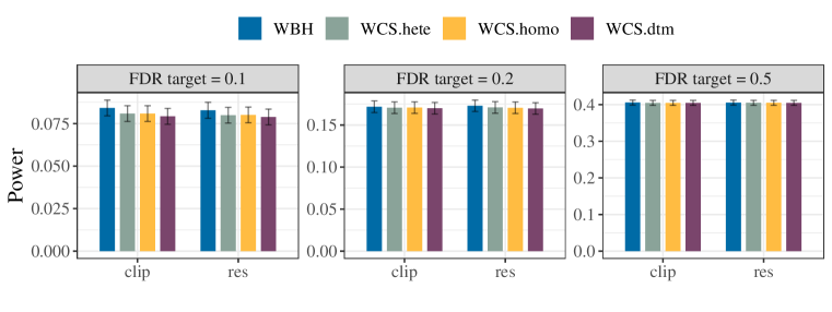
Figure 3: Empirical power for drug property prediction. Everything else is as in Figure 2.

4.2 Drug-target interaction prediction

We then consider drug-target interaction (DTI) prediction, where the goal is to select drug-target pairs with a high binding score. This task is relevant if a therapeutic company is interested in prioritizing resources for drug candidates that may be effective for any target they are interested in. We use the DAVIS dataset [DHH⁺11], which records real-valued binding affinities for $n_{\textrm{tot}}=30060$ drug-target pairs. The drugs and the targets are encoded into numeric features using ECFP and Conjoint triad feature (CTF) [SZL⁺07, STW⁺09].

We essentially follow the same procedure as in Section 4.1 and only rehearse the main components. First, we randomly sample a subset of size $n_{\textnormal{train}}=0.2\times n_{\textrm{tot}}$ as $\mathcal{D}_{\textnormal{train}}$, on which we train a regression model $\widehat{\mu}(\cdot)\colon\mathcal{X}\to\mathbb{R}$ using a $3$-layer neural network with $10$ training epochs. This relatively simple model is suitable for numerical experiments on CPUs (one can surely use more complicated prediction models in practice). As before, we use the same model $\widehat{\mu}(\cdot)$ for both predicting test samples and selecting calibration data into first-batch screening (in practice, they can of course be different). We sample a drug-target pair for inclusion in the calibration set with probability $p(x)=\sigma(2\widehat{\mu}(x)-\bar{\mu})$, where $\bar{\mu}$ is the average training prediction as before. Finally, among those not selected in the calibration data, we randomly sample a subset of size $m=5000$ as test data.

We choose a more complicated threshold $c_{j}$ for the continuous response. For a drug-target pair $X_{n+j}$, we set $c_{j}$ to be the $q_{\textrm{pop}}$-th quantile of the binding scores of all drug-target pairs in $\mathcal{D}_{\textnormal{train}}$ with the same target. We evaluate $q_{\textrm{pop}}\in\{0.7,0.8\}$. Thus, $c_{j}:=c(X_{n+j},\mathcal{D}_{\textnormal{train}},q_{\textrm{pop}})$ where $c$ is a mapping that takes both $\mathcal{D}_{\textnormal{train}}$ and the target information in $X_{n+j}$ as inputs. Lastly, we evaluate the BH procedure and Algorithm 1 with scores:

• res: $V(x,y)=y-\widehat{\mu}(x)$.

• clip: $V(x,y)=M\cdot\operatorname{\mathds{1}}\{y>c(x,\mathcal{D}_{\textnormal{train}},q_{\textrm{pop}})\}+c(x,\mathcal{D}_{\textnormal{train}},q_{\textrm{pop}})\operatorname{\mathds{1}}\{y\leq c(x,\mathcal{D}_{\textnormal{train}},q_{\textrm{pop}})\}-\widehat{\mu}(x)$ in which $M=100$.

We always use $\mathcal{D}_{\textnormal{calib}}$ as the calibration set, and set the FDR target as $q\in\{0.1,0.2,0.5\}$.

Figure 4 shows false discovery proportions (FDPs) for $q_{\textrm{pop}}=0.8$ in $N=200$ independent. Similar results for $q_{\textrm{pop}}=0.7$ are presented in Appendix A.5. We see that the FDR is controlled at the desired level for all algorithms and nonconformity scores. This shows the validity of our algorithms and the plausibility of the independence assumptions we make on the drug-target pairs. In this task, we do not observe much difference between deterministic pruning (WCS.dtm) and the other two pruning options. Furthermore, we observe that the FDPs across replications tightly concentrate especially for clip and $q\in\{0.2,0.5\}$, showing that our algorithms are stable with respect to data splitting (i.e., the randomness in choosing the initial screening sets and in the training process). Comparing the two nonconformity scores, we see that clip exploits the error budget and obtains a realized FDR, which is very close to the nominal level, while res has a much lower FDR in all cases. Not surprisingly, Figure 5 shows that clip has much higher power.

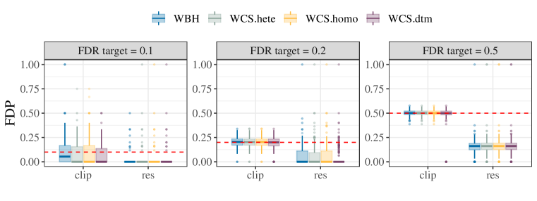
Figure 4: Empirical FDR for drug-target interaction prediction with $q_{\textrm{pop}}=0.8$. The shorthand WBH stands for BH procedure, and WCS.* for Algorithm 1 with three pruning options $*\in\{\texttt{hete},\texttt{homo},\texttt{dtm}\}$. The red dashed lines are the nominal FDR levels. Solid lines are empirical averages (here empirical FDR).

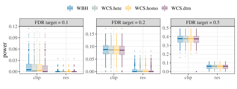
Figure 5: Empirical power for drug-target interaction prediction with $q_{\textrm{pop}}=0.8$. Everything else is as in Figure 4.

5 Application to multiple individual treatment effects

We now apply our method to infer individual treatment effects (ITEs) [LC21, JRC23] under the potential outcomes framework [IR15]. The ITE describes the difference between an individual’s outcomes when receiving a treatment versus not; its variation comes from both individual characteristics and intrinsic uncertainty in the outcomes. Inference on multiple ITEs is useful in assisting reliable personalized decision making.

We consider a super-population setting, where $(X_{i},O_{i}(1),O_{i}(0),T_{i})$ are drawn i.i.d. from a joint distribution $\mathcal{P}$ (distinct from the distributions $P$ and $Q$ we use for the data). Here, $X_{i}\in\mathcal{X}$ is the features, $T_{i}\in\{0,1\}$ indicates whether unit $i$ receives treatment, and $O_{i}(1),O_{i}(0)$ are the potential outcomes under treatment and not, respectively. Under the standard SUTVA [IR15], we observe $(X_{i},O_{i},T_{i})$, where $O_{i}=O_{i}(T_{i})=T_{i}O_{i}(1)+(1-T_{i})O_{i}(0)$. We will specify how the treatment $T_{i}$ is allocated later on. We focus on units in the study, i.e., those who have received a certain treatment option. The ITE of unit $i$ is the random variable $\Delta_{i}=O_{i}(1)-O_{i}(0)$. As only one potential outcome is observed, a crucial part of inferring the ITE is to predict the counterfactual, i.e., $O_{i}(1)$ for those units with $T_{i}=0$, and $O_{i}(0)$ for $T_{i}=1$. In the following, we consider simultaneous inference for the ITEs of a set of units in the control group (inference for treated units is similar).

Formally, the test samples are $\{X_{n+j}\}_{j=1}^{m}$ are units in the control group (the outcome $O_{n+j}$ is observed). Our goal is to screen for positive ITEs with FDR control, i.e., finding a subset $\mathcal{R}\subseteq\{1,\dots,m\}$, such that

$$\textnormal{FDR}:=\mathbb{E}\Bigg{[}\frac{\sum_{j=1}^{m}\operatorname{\mathds{1}}\{O_{n+j}(1)\leq O_{n+j}(0),~{}j\in\mathcal{R}\}}{1\vee|\mathcal{R}|}\Bigg{]}\leq q.$$ (12)

To cast the counterfactual problem in our framework, set $Y_{n+j}:=O_{n+j}(1)$ to be the unobserved outcome, and the thresholds $c_{n+j}:=O_{n+j}(0)$ to be the observed outcomes. To infer $Y_{n+j}$, the training data is $\{(X_{i},Y_{i})\}_{i=1}^{n}=\{(X_{i},O_{i}(1))\}_{i=1}^{n}$ for which $T_{i}=1$. Conditional on the treatment status, the training samples are i.i.d. from $P:=\mathcal{P}_{X,O(1){\,|\,}T=1}$, while the test samples $\{(X_{n+j},Y_{n+j})\}_{j=1}^{m}$ are i.i.d. from $Q:=\mathcal{P}_{X,O(1){\,|\,}T=0}$. The relationship between $P$ and $Q$ will depend on the treatment assignment mechanism.

5.1 Warm-up: completely randomized experiments

As a warmup, consider a completely randomized experiment, where the treatment assignments $T_{i}$ are i.i.d. draws from $\textrm{Bern}(\pi)$ for some $\pi\in(0,1)$ independently from everything else. In this case, $P=Q=\mathcal{P}_{X,O(1)}$ and it suffices to use conformal p-values without weights. The testing procedure for randomized experiments has already been studied in [JC22]. Take any monotone nonconformity score $V(\cdot,\cdot)$ obtained from an independent training process, and compute $V_{i}=V(X_{i},O_{i})=V(X_{i},O_{i}(1))$ for $i=1,\dots,n$, and $\widehat{V}_{n+j}=V(X_{n+j},O_{n+j})=V(X_{n+j},O_{n+j}(0))$ for $j=1,\dots,m$. Then construct conformal p-values (5) with $w(\cdot)\equiv 1$, and run the BH procedure with these p-values at level $q$. FDR control is a corollary of [JC22, Theorem 2.3], and we omit the proof.

Corollary 5.1.

The procedure above has FDR (12) at most $q$.

5.2 Stratified randomization and observational studies

We now consider a more general setting where the treatment assignment may depend on the observed covariates, formalized as the following strong ignorability condition [IR15].

Assumption 5.2 (Strong ignorability).

Under the joint distribution $\mathcal{P}$, it holds that $(O(1),O(0))\perp\!\!\!\perp T{\,|\,}X$. Equivalently, the treatment assignments are independently generated from $T_{i}\sim\textrm{Bern}(e(X_{i}))$, where $e\colon\mathcal{X}\to(0,1)$ is known as the propensity score.

Assumption 5.2 is automatically satisfied in stratified randomization experiments, where the treatment is randomized in a way that only depends on the covariates, and the propensity score $e(\cdot)$ is known. In observational studies where the treatment assignment mechanism is completely unknown, Assumption 5.2 is standard for the identifiability of average treatment effects [Ros02]. Inference on ITEs when this assumption is violated (i.e., when there is unmeasured confounding) is studied in [JRC23]; that said, multiple testing under confounding needs additional techniques, and is beyond the scope of the current work.

Under Assumption 5.2, the covariate shift condition (1) holds [LC21], as

$$\frac{{\,\mathrm{d}}Q}{{\,\mathrm{d}}P}(x,y)=\frac{{\,\mathrm{d}}\mathcal{P}_{X,O(1){\,|\,}T=0}}{{\,\mathrm{d}}\mathcal{P}_{X,O(0){\,|\,}T=1}}(x,y)=\frac{{\,\mathrm{d}}\mathcal{P}_{X{\,|\,}T=0}}{{\,\mathrm{d}}\mathcal{P}_{X{\,|\,}T=1}}(x)=w(x):=\frac{\pi(1-e(x))}{(1-\pi)e(x)},$$

where $e(x)=\mathcal{P}(T=1{\,|\,}X=x)$ is the propensity score, and $\pi=\mathcal{P}(T=1)$ is the marginal probability of being treated. As such, Algorithm 1 is readily applicable when $e(\cdot)$ is known.

Corollary 5.3.

Suppose $e(\cdot)$ is known, and Assumption 5.2 holds. Consider calibration data $\{(X_{i},O_{i}(1)\colon T_{i}=1\}_{i=1}^{n}$, test data $\{X_{n+j}\colon T_{n+j}=1\}_{j=1}^{m}$, thresholds $\{O_{n+j}(0)\colon T_{n+j}=0\}_{j=1}^{m}$, any monotone score $V$, and weight function $w(x)\propto(1-e(x))/{e(x)}$ as the input of Algorithm 1. Then any selection procedure $\mathcal{R}\in\{\mathcal{R}_{\textnormal{hete}},\mathcal{R}_{\textnormal{homo}},\mathcal{R}_{\textnormal{dtm}}\}$ has FDR at most $q$.

The propensity score function $e(\cdot)$ is unknown for observational data. Under Assumption 5.2, we can estimate the propensity scores (hence the weight function) using an independent training fold and plug this estimate into the construction of p-values. As a corollary of Theorem 3.5, we can develop an FDR bound for observational data.

Corollary 5.4.

In the setting of Corollary 5.3, take $w(x)\propto(1-\widehat{e}(x))/{\widehat{e}(x)}$ as the input of Algorithm 1, where $\widehat{e}(\cdot)$ is an estimate of $e(\cdot)$ which is independent of the calibration and training data. Then any selection procedure $\mathcal{R}\in\{\mathcal{R}_{\textnormal{hete}},\mathcal{R}_{\textnormal{homo}},\mathcal{R}_{\textnormal{dtm}}\}$ obeys

$$\textnormal{FDR}\leq q\cdot\mathbb{E}\bigg{[}\frac{\widehat{\gamma}^{2}}{1+q(\widehat{\gamma}^{2}-1)/m}\bigg{]},\qquad\widehat{\gamma}:=\sup_{x\in\mathcal{X}}\max\bigg{\{}\frac{1-e(x)\widehat{e}(x)}{e(x)(1-\widehat{e}(x))},\frac{e(x)(1-\widehat{e}(x))}{1-e(x)\widehat{e}(x)}\bigg{\}}.$$

At a high level, the conformal p-values compare the observed outcome $O_{n+j}(0)$ of the control units to the empirical distribution of $O_{i}(1)$ in the calibration data; the latter—after proper weighting—shows the typical behavior of the counterfactual $O_{n+j}(1)$, and provides evidence for whether it may be larger than $O_{n+j}(0)$, i.e., whether $\Delta_{n+j}$ is positive.

In predicting $O_{n+j}(1)$, we use the marginal distribution of $(X,O(1))$ from the calibration data, but ignore the information in the observed outcome $O(0)$. Put differently, our inference for ITEs is valid regardless of how the potential outcomes are coupled. Thus, the actual false discovery rate may be lower than $q$. Indeed, it is observed in [JRC23] that the FDR for identifying positive ITEs—even without adjusting for multiplicity—can sometimes be lower than the nominal level. Next, we are to empirically investigate the FDR and power of our method under various couplings of potential outcomes. A theoretical understanding is left for future work.

5.3 Simulation studies

We design joint distributions of the variables $(X,O(1),O(0),T)$ with various covariate distributions, regression functions, and couplings of potential outcomes. The covariates $X_{i}\in\mathbb{R}^{10}$ ($p=10$) are obtained via $X_{ij}=\Phi(X_{ij}^{0})$, $j=1,\dots,10$, where $X_{i}^{0}\in\mathbb{R}^{10}$ are i.i.d. $\mathcal{N}(0,\Sigma)$, and $\Phi(\cdot)$ is the CDF of a $\mathcal{N}(0,1)$ random variable. We set $\Sigma=I_{p}$ for the independent case and $\Sigma_{k,j}=0.9^{|k-j|}$ for the correlated case. We consider three cases:

• Setting 1: $O_{i}(0)=0.1\,\epsilon_{0,i}$, $O_{i}(1)=\max\{0,\mu_{1}(X_{i})+\sigma_{1}(X_{i})\,\epsilon_{1,i}\}$, where $\sigma_{1}(x)=0.2-\log x_{1}$ and $\mu_{1}(x)={4}/{(1+e^{-12x_{1}-0.5})(1+e^{-12x_{2}-0.5})}$.

• Setting 2 is a mixture of deterministic and stochastic ITEs. With probability $0.1$, set $O_{i}(1)=0.1\,\epsilon_{0,i}-0.5$, and $O_{i}(0)=O_{i}(1)+0.05$; otherwise, set them as in Setting 1.

• Setting 3: $O_{i}(0)=\mu_{0}(X_{i})+0.1\,\epsilon_{0,i}$, $O_{i}(1)=\max\{0,\mu_{1}(X_{i})+\sigma_{1}(X_{i})\,\epsilon_{1,0}\}$, where $\sigma_{1}(\cdot)$ is as in Setting 1, and $\mu_{0}(x)={2}/{(1+e^{-3x_{1}-0.5})(1+e^{-3x_{2}-0.5})}$, $\mu_{1}(x)=0.1+1.5\,\mu_{0}(x)$.

Above, the variables ($\epsilon_{0,i},\epsilon_{1,i}$) are i.i.d. with $\mathcal{N}(0,1)$ as marginals. We consider three coupling scenarios: (i) independent, in which $\epsilon_{0,i}$ and $\epsilon_{1,i}$ are independent; (ii) negative, in which $\epsilon_{1,i}=-\epsilon_{0,i}$; (iii) positive, in which $\epsilon_{1,i}=\epsilon_{0,i}$. We generate treatment indicators via $T_{i}\sim\textrm{Bern}(e(X_{i}))$ independently, where $e(x)=(1+\textrm{Beta}_{2,4}(x_{1}))/{4}$, and $\textrm{Beta}_{2,4}(\cdot)$ is the CDF of the Beta distribution with shape parameters $(2,4)$. Finally, we set those $T_{i}=1$ as the calibration data ($n=250$), and those $T_{i}=0$ as the test sample ($m=100$); as training data we select $n_{\textnormal{train}}=750$ units, which are used to construct four conformity scores:

• reg: $V(x,y)=y-\widehat{\mu}(x)$, where $\widehat{\mu}(x)$ is an estimate of $\mu_{1}(x)$ using regression forest from the grf R-package [ATW19].

• cdf: $V(x,y)=\widehat{F}(x,y)$ [CWZ21], where $\widehat{F}(x,y)$ is an estimate of $\mathcal{P}(O(1)\leq y{\,|\,}X=x)$. Here, we fit $\widehat{F}$ via inverting quantile regression forests from grf.

• oracle: $V(x,y)=\mathcal{P}(O(1)\leq y{\,|\,}X=x)$, which is not computable from data and is shown only for illustration.

• cqr: $V(x,y)=y-\widehat{q}_{\beta}(x)$ [RPC19], where $\widehat{q}_{\beta}(x)$ is an estimate of the $\beta$-th quantile of $\mathcal{P}_{O(1){\,|\,}X=x}$, $\beta\in\{0.2,0.5,0.8\}$, from the quantile regression forests in grf.

After generating the three folds of data, we fit $V(\cdot,\cdot)$ on the training fold, and run four procedures on the calibration and training folds: BH with weighted conformal p-values in (4) (named WBH in the plot), and Algorithm 1 with three pruning options (named WCS.hete, WCS.homo, WCS.dtm, respectively). The experiment is repeated for $N=1000$ independent runs.

Among the three, setting 2 is the most challenging: $10\%$ of the samples are with slightly negative ITEs; they are likely to be falsely rejected since the selection procedure ignores the coupling (it may reject a sample with a small value of $O(0)$ even if $O(1)$ is smaller). We expect setting 1 to be the least challenging as there is a strong signal in $O(1)$. Setting 3 is more challenging than setting 1 since $O(1)$ and $O(0)$ are close to each other as the regression functions are similar.

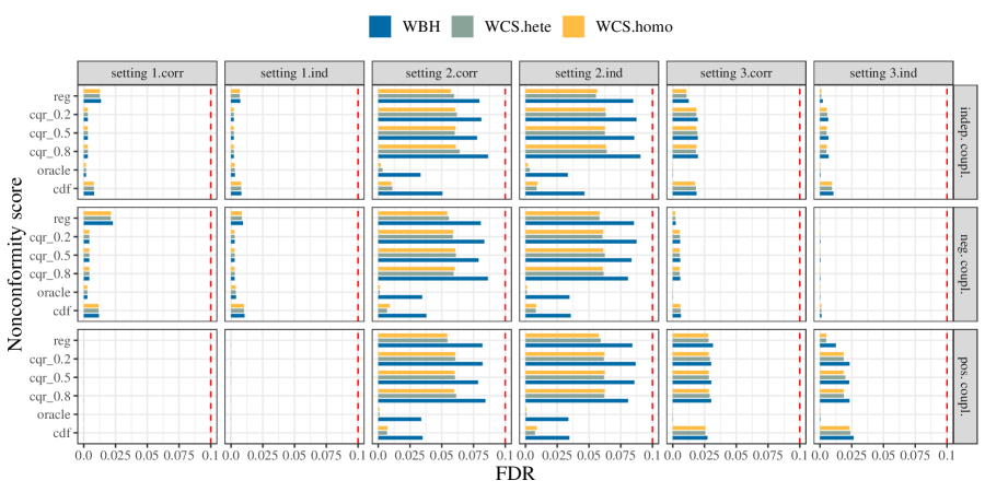
Figure 6: Empirical FDR for finding positive ITEs. The columns represent three settings with either independent (ind) or correlated (corr) covariates. Each row corresponds to a coupling of potential outcomes (positive, negative, and no coupling). In each subplot, the $y$-axis is the nonconformity score, and the $x$-axis is the empirical FDR. The red dashed lines indicate the nominal level $q=0.10$.

FDR control.

The empirical FDR in all settings is plotted in Figure 6. We observe FDR control for all methods, including the BH procedure. (We omit the results of $\mathcal{R}_{\textnormal{dtm}}$ because it does not succeed in making any selection.) Across settings with the same regression function, those with correlated covariates often have higher FDR. The realized FDR also varies with the scores: oracle incurs very low FDR, while its empirical counterpart cdf has higher FDR. On the other hand, quantile regression based scores are robust to the quantile level $\beta$ in the sense that cqr achieves similar FDR for all choices of $\beta$.

The impact of coupling on FDR is less consistent across settings. The positive coupling from setting 1 yields a low FDR, perhaps because it is difficult to obtain sufficiently strong evidence which leads to fewer rejections (see the power analysis below). The three couplings yield similar FDRs for setting 2. For setting 3, positive coupling leads to the highest FDR.

Power.

The empirical power is defined as $\textrm{Power}:=\mathbb{E}\Big{[}\frac{\sum_{j=1}^{m}\operatorname{\mathds{1}}\{j\in\mathcal{R},O_{n+j}(1)>O_{n+j}(0)\}}{\sum_{j=1}^{m}\operatorname{\mathds{1}}\{O_{n+j}(1)>O_{n+j}(0)\}}\Big{]}.$ As we see in Figure 7, the power is in general higher when the covariates are correlated. The ITE depends on $(X_{1},X_{2})$, and in our design, higher correlation between the first two entries leads to higher power. The power also varies with the nonconformity scores. The regression-based reg leads to lower power than other methods. This means that regression functions may be underpowered in capturing the essential information for contrasting the distributions of two potential outcomes. Quantile-regression based methods (cqr) achieve similar power for different choices of $\beta$ in all settings. Finally, fitting the conditional distribution function (cdf) is the most powerful option in settings 1 and 3, but is far less powerful in setting 2. Its oracle version (oracle) is also surprisingly less powerful; we observe that the oracle cdf cannot create sufficiently small p-values, while the estimated one is able to do so due to fluctuations caused by estimation uncertainty.

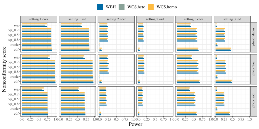
Figure 7: Empirical power for finding positive ITEs. Everything else is as in Figure 6.

The impact of coupling on the power is consistent across settings. In general, negative coupling leads to the highest power, while positive coupling leads to the lowest. This is because the conformal p-values compare the observed outcome to the marginal distribution of the counterfactuals, without accounting for their joint distribution. Thus, when $O_{n+j}(0)$ is extremely small, i.e., when we see a small p-value and $j\in\mathcal{R}$, under negative coupling, it is more probable that $O_{n+j}(1)$ is relatively large, hence leading to a true discovery. On the contrary, under positive coupling, a large $O_{n+j}(1)$ often corresponds to a relatively large $O_{n+j}(0)$ and hence a large conformal p-value, which may not be selected.

Finally, $\mathcal{R}_{\textnormal{dtm}}$ makes no selection. This may be due to the threshold effect: since the selection requires $p_{j}\leq q|\widehat{\mathcal{R}}_{j\to 0}|/m$ for test samples $j$ with the smallest $|\widehat{\mathcal{R}}_{j\to 0}|$, the pruning step may exclude too many candidates. We recommend using $\mathcal{R}_{\textnormal{hete}}$ and $\mathcal{R}_{\textnormal{homo}}$ in practice.

Stability.

As aforementioned in Section 3, our method introduces extra randomness. It is shown in Proposition 3.4 that this becomes asymptotically negligible, so that our selection set is asymptotically the same as that the BH procedure yields. We empirically evaluate the discrepancy in the selections, namely, $|\mathcal{R}\Delta\mathcal{R}_{\textnormal{BH}}|/|\mathcal{R}_{\textnormal{BH}}|$, for $\mathcal{R}$ being either $\mathcal{R}_{\textnormal{homo}}$ or $\mathcal{R}_{\textnormal{hete}}$. The results are shown in Figure 8, confirming our theory. Though we were not able to prove the asymptotic equivalence of $\mathcal{R}_{\textnormal{hete}}$ and $\mathcal{R}_{\textnormal{BH}}$ in the $m,n\to\infty$ regime, the discrepancy is still small (despite being larger than that of $\mathcal{R}_{\textnormal{homo}}$). All in all, the impact of additional randomness seems acceptable in practice.

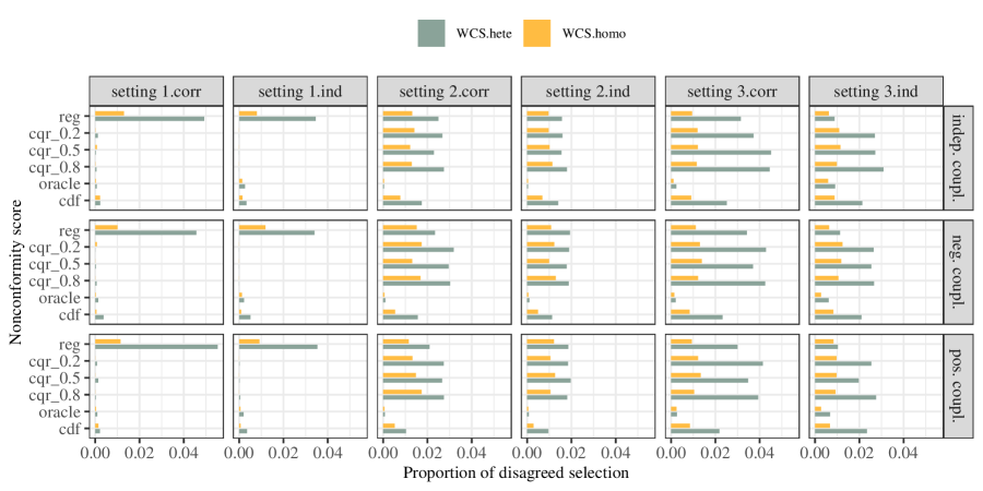
Figure 8: Discrepancy between selection rules $|\mathcal{R}\Delta\mathcal{R}_{\textnormal{BH}}|/|\mathcal{R}_{\textnormal{BH}}|$. Everything else is as in Figure 6.

The discrepancy for $\mathcal{R}_{\textnormal{dtm}}$ from $\mathcal{R}_{\textnormal{BH}}$ is large in general is $\mathcal{R}_{\textnormal{dtm}}$ is usually an empty set, and hence we did not plot it. We conjecture that the stability of $\mathcal{R}_{\textnormal{dtm}}$ claimed in case (i) from Proposition 3.4 may not necessarily apply to the moderately large sample sizes $m=100$ and $n=250$, and $\mathcal{R}_{\textnormal{dtm}}$ may be far from $\mathcal{R}_{\textnormal{BH}}$ for such sample sizes. In such cases, we recommend using $\mathcal{R}_{\textnormal{homo}}$ or $\mathcal{R}_{\textnormal{hete}}$ for better stability and power.

5.4 Real data analysis

We revisit the NSLM observational dataset from [CFM⁺19] and use our method to detect multiple positive individual treatment effects. It is a semi-synthetic observational dataset curated from a real randomized experiment, also analyzed in [LC21, JRC23].

Figure 2 in [JRC23] plots the $\Gamma$-value, a measure of robustness of positive ITEs against unmeasured confounding, versus individual covariates. While units with larger $\Gamma$-values are of natural interest, properties of inference hold on average, instead of over selected units (e.g. those with high $\Gamma$-values). We are to produce a similar plot (Figure 10) for detecting positive ITEs, with guarantees over units that exhibit the strongest evidence. (We do not consider the confounding issue, which may need nontrivial extension of our techniques.)

We randomly subsample three disjoint folds of size $5000$, $1000$, and $391$ from the original dataset. The first is the training fold, and consists of both treated and control units. The calibration data consists of all the $n=997$ treated units in the second fold. The test data consists of all the $m=256$ control units in the last fold. To deploy our procedure, we first train a propensity score model $\widehat{e}(\cdot)$ using a regression forest from the grf R-package, and set $\widehat{w}(x)=(1-\widehat{e}(x))/{\widehat{e}(x)}$. We then use a quantile regression forest from grf on the training data to fit $\widehat{q}_{0.5}(x)$, the conditional median of $O(1)\mid X$, and set $V(x,y)=y-\widehat{q}_{0.5}(x)$. Finally, we apply Algorithm 1 as in Theorem 3.1 to test for positive ITEs.

Figure 9 plots the empirical CDF of the weighted conformal p-values (5) computed with $c_{n+j}:=O_{n+j}(0)$ on the test samples. These p-values are stochastically smaller than Unif([0,1]), showing evidence for positive treatment effects in general. Yet, to identify positive ITEs with rigorous error control we must apply multiple testing ideas here.

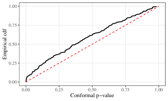
Figure 9: Empirical CDF of the weighted conformal p-values for detecting positive ITEs.

We observe $\mathcal{R}_{\textnormal{BH}}=\mathcal{R}_{\textnormal{homo}}=\mathcal{R}_{\textnormal{hete}}$ while $\mathcal{R}_{\textnormal{dtm}}=\varnothing$ at FDR levels $q\in\{0.1,0.2,0.5\}$. Figure 10 plots the weighted conformal p-values versus school achievement levels of test units (each dot represents a test unit) with red dots (from light to dark) identified as positive ITEs at various FDR levels. Students in schools with moderate achievement levels demonstrate the strongest evidence of benefiting from the treatment.

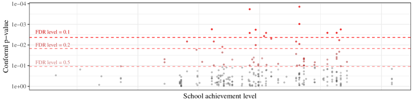
Figure 10: P-values and rejection sets for detecting positive ITEs among control units.

6 Application to outlier detection

Finally, we study the extension of our framework for outlier detection, where the calibration inliers may follow a distinct distribution compared with test inliers. We discuss a new setup and apply a variant of Algorithm 1 to bank marketing data.

6.1 Hypothesis-conditional FDR control

Assuming access to i.i.d. training data $\{Z_{i}\}_{i=1}^{n}$, we consider a set of test data $\{Z_{n+j}\}_{j=1}^{m}$ for which the $Z_{n+j}$’s may only be partially observed (e.g., if $Z=(X,Y)$ we would observe the features $X$ but not the response $Y$). We are interested in some null hypotheses $\{H_{j}\}_{j=1}^{m}$ associated with the test samples. As before, whether $H_{j}$ is true can be a random event depending on $Z_{n+j}$; this includes our previous problem with $H_{j}\colon Y_{n+j}\leq c_{n+j}$.

6.1.1 Hypothesis-conditional covariate shift

Assumption 6.1 (Hypothesis-conditional covariate shift).

$\{Z_{i}\}_{i=1}^{n}\cup\{Z_{n+j}\}_{j=1}^{m}$ are mutually independent. Also, conditional on the subset $\mathcal{H}_{0}\subset\{1,\dots,m\}$ of all null hypotheses, it holds that $\{Z_{i}\}_{i=1}^{n}\stackrel{{\scriptstyle\textnormal{i.i.d.}}}{{\sim}}P$, and $\{Z_{n+j}\}_{j\in\mathcal{H}_{0}}\stackrel{{\scriptstyle\textnormal{i.i.d.}}}{{\sim}}Q$, where ${\,\mathrm{d}}Q/{\,\mathrm{d}}P(Z)=w(X)$ for some function $w\colon\mathcal{X}\to\mathbb{R}^{+}$ and $X\subseteq Z$.

A special case of problem (2) obeys these assumptions.

Example 6.2 (Binary classification).

Set $Z=(X,Y)$. where $Y\in\{0,1\}$ is a binary response. Suppose the goal is to find positive $Y_{n+j}$, e.g. an active drug or a qualified candidate. We only observe the covariates $\{X_{n+j}\}_{j=1}^{m}$ for the test samples $\{(X_{n+j},Y_{n+j})\}_{j=1}^{m}\stackrel{{\scriptstyle\textnormal{i.i.d.}}}{{\sim}}Q$. Consider a reference dataset that only preserves positive samples among a set of i.i.d. data from a covariate shifted distribution $P$ ; that is, $\mathcal{D}_{\textnormal{calib}}=\{Z_{i}\colon Y_{i}=0\}$ where $\{(X_{i},Y_{i})\}\stackrel{{\scriptstyle\textnormal{i.i.d.}}}{{\sim}}P$. Although the (super-population) covariate shift (1) no longer applies, conditional on $\mathcal{H}_{0}=\{j\colon Y_{n+j}=0\}$, it still holds that $Z_{i}\stackrel{{\scriptstyle\textnormal{i.i.d.}}}{{\sim}}P_{Z{\,|\,}Y=0}$ for $Z_{i}\in\mathcal{D}_{\textnormal{calib}}$, and $Z_{n+j}\stackrel{{\scriptstyle\textnormal{i.i.d.}}}{{\sim}}Q_{Z{\,|\,}Y=0}$ for $j\in\mathcal{H}_{0}$.

The above example also applies to candidate screening with constant thresholds $c_{n+j}\equiv c_{0}$. Setting $\widetilde{Y}=\operatorname{\mathds{1}}\{Y>c_{0}\}\in\{0,1\}$ and $\mathcal{D}_{\textnormal{calib}}=\{Z_{i}\colon Y_{i}\leq c_{0}\}$, all arguments apply similarly to $\widetilde{Z}=(X,\widetilde{Y})$. However, this does not necessarily apply when the thresholds $c_{n+j}$ are random variables (especially when no ’threshold $c_{j}$’ is observed in the calibration data, such as in the counterfactual inference problem we will study later).

Another application is outlier detection under covariate shifts.

Example 6.3 (Outlier detection).

We revisit outlier detection [BCL⁺21] while allowing for identifiable covariate shifts between the calibration inliers and the test inliers. Given $\{Z_{i}\}_{i=1}^{n}$ drawn i.i.d. from an unknown distribution $P$ and a set of test data $\{Z_{n+j}\}_{j=1}^{m}$, we assume the inliers in the test data are i.i.d. from a distribution $Q$ with ${\,\mathrm{d}}Q/{\,\mathrm{d}}P(Z)=w(Z)$ for a known function $w$, while allowing outliers to be from arbitrary distributions. The covariate shift may happen, for example, when inliers were from $Q$ but the calibration set is selected with preferences relying on $z$: for instance, one may include more female users to balance the gender distribution when curating a reference panel of normal transactions (inliers). In this case, $\mathcal{H}_{0}=\{j\colon Z_{n+j}\sim Q\}$ is a deterministic set, and Assumption 6.1 clearly holds.

The outlier detection example is closely related to identifying concept drifts.

Example 6.4 (Concept shift detection).

Letting $Z=(X,Y)$ where $X\in\mathcal{X}$ is the family of covariates and $Y$ is the response, concept shift focuses on potential changes in the conditional distribution of $Y$ given $X$. Given calibration data $\{Z_{i}\}_{i=1}^{n}\stackrel{{\scriptstyle\textnormal{i.i.d.}}}{{\sim}}P$ and independent test data $\{Z_{n+j}\}_{j=1}^{m}$, [HL20] assume $\{Z_{n+j}\}_{j=1}^{m}\stackrel{{\scriptstyle\textnormal{i.i.d.}}}{{\sim}}Q$, and test for the global null $H_{0}\colon{\,\mathrm{d}}Q/{\,\mathrm{d}}P(Z)=w(X)$ for some $w\colon\mathcal{X}\to\mathbb{R}^{+}$. They achieve this by combining independent p-values after sample splitting. Our framework can be used to test individual concept drifts with dependent p-values. For instance, assume $\{X_{n+j}\}_{j=1}^{m}\stackrel{{\scriptstyle\textnormal{i.i.d.}}}{{\sim}}Q_{X}$ for some unknown (but estimable) $Q_{X}$, we can test whether $P_{Y_{n+j}{\,|\,}X_{n+j}}=P_{Y{\,|\,}X}$. The null hypotheses can be formulated as $H_{j}\colon Z_{n+j}\sim Q$, where ${\,\mathrm{d}}Q/{\,\mathrm{d}}P(Z)=w(X)$ for some $w\colon\mathcal{X}\to\mathbb{R}^{+}$ that is either known or can be estimated well under proper conditions.

6.1.2 Multiple testing procedure

Our procedure for outlier detection under covariate shift is detailed in Algorithm 2. This slightly modifies Algorithm 1 by removing the thresholds (note differences in lines 1, 2, and 4). In the classification or constant threshold problem (Example 6.2), it suffices to set $Z=X$ and leave out $Y$.

Algorithm 2 Hypothesis-conditional Weighted Conformalized Selection

0:  Calibration data $\{Z_{i}\}_{i=1}^{n}$, test data $\{Z_{n+j}\}_{j=1}^{m}$, weight function $w(\cdot)$, FDR target $q\in(0,1)$, monotone nonconformity score $V\colon\mathcal{X}\times\mathcal{Y}\to\mathbb{R}$, pruning method $\in\{\texttt{hete},\texttt{homo},\texttt{dtm}\}$.

1:  Compute $V_{i}=V(Z_{i})$ for $i=1,\dots,n$, and ${V}_{n+j}=V(Z_{n+j})$ for $j=1,\dots,m$.

2:  Construct weighted conformal p-values $\{p_{j}\}_{j=1}^{m}$ as in (5) with $\widehat{V}_{n+j}$ replaced by $V_{n+j}$. - First-step selection -

3:  for $j=1,\dots,m$ do

4:     Compute p-values $\{{p}_{\ell}^{(j)}\}$ as in (6) with $\widehat{V}_{n+\ell}$ replaced by $V_{n+\ell}$ for all $\ell=1,\dots,m$.

5:     (BH procedure) Compute $k^{*}_{j}=\max\big{\{}k\colon 1+\sum_{\ell\neq j}\operatorname{\mathds{1}}\{{p}_{\ell}^{(j)}\leq qk/m\}\geq k\big{\}}$.

6:     Compute $\widehat{\mathcal{R}}_{j\to 0}=\{j\}\cup\{\ell\neq j\colon{p}_{\ell}^{(j)}\leq qk^{*}_{j}/m\}$.

7:  end for

8:  Compute the first-step selection set $\mathcal{R}^{(1)}=\{j\colon{p}_{j}\leq q|\widehat{\mathcal{R}}_{j\to 0}|/m\}$. - Second-step selection -

9:  Compute $\mathcal{R}=\mathcal{R}_{\textrm{hete}}$ or $\mathcal{R}=\mathcal{R}_{\textrm{homo}}$ or $\mathcal{R}=\mathcal{R}_{\textrm{dtm}}$ as in Algorithm 1.

9:  Selection set $\mathcal{R}$.

Algorithm 2 returns to the conventional perspective, where the null set is deterministic, and the null p-values are dominated by Unif$([0,1])$. That is, for $p_{j}$ constructed in Line 2 of Algorithm 2, it holds that

$$\mathbb{P}(p_{j}\leq t{\,|\,}j\in\mathcal{H}_{0})\leq t\quad\textrm{for all }t\in[0,1].$$

After conditioning on $\mathcal{H}_{0}$, we no longer need to deal with the randomness of the hypotheses and their interaction with the p-values. The only issue is the mutual dependence among the p-values, which is addressed using a similar idea as in our theoretical analysis of Algorithm 1.

Using calibration data obeying the covariate shift assumption, Algorithm 2 achieves a slightly stronger hypotheses-conditional FDR control. The proof of Theorem 6.5 is in Appendix C.5.

Theorem 6.5.

Under Assumption 6.1, Algorithm 2 yields

$$\mathbb{E}\bigg{[}\frac{|\mathcal{R}\cap\mathcal{H}_{0}|}{1\vee|\mathcal{R}|}\,\bigg{|}\,\mathcal{H}_{0}\bigg{]}\leq q\cdot\frac{|\mathcal{H}_{0}|}{m}$$

for any fixed $q\in(0,1)$, and each $\mathcal{R}\in\{\mathcal{R}_{\textnormal{homo}},\mathcal{R}_{\textnormal{hete}},\mathcal{R}_{\textnormal{dtm}}\}$.

6.1.3 Comparison with Algorithm 1

In binary classification, or more generally, WCS with a constant threshold, we have shown in Example 6.2 that Algorithm 2 yields FDR control. In this case, Algorithms 1 and 2 differ in terms of (i) power, and (ii) distributional assumptions. We elaborate on these distinctions.

First, Algorithm 2 only uses a subset of calibration data to construct p-values, which leads to a power loss for specific choices of nonconformity scores; see [JC22, Appendix A.1] for the i.i.d. case. Let us consider the binary setting. Suppose we have access to a set of calibration data $\{(X_{i},Y_{i})\}$ consisting of both $Y=1$ and $Y=0$ samples. As discussed in Example 6.2, Assumption 2 holds if we only use data in the subset $\mathcal{I}_{0}=\{i\colon Y_{i}=0\}$ as $\mathcal{D}_{\textnormal{calib}}$ in Algorithm 2. In contrast, Algorithm 1 uses all data points. Suppose we set $V(x,y)=My-\widehat{\mu}(x)$ and $c_{n+j}\equiv 0$ in Algorithm 1, where $\widehat{\mu}(\cdot)$ is a fitted point prediction, and $M>2\sup_{x\in\mathcal{X}}|\widehat{\mu}(x)|$ is a sufficiently large constant. Similarly, we set $V(x)=M-\widehat{\mu}(x)$ in Algorithm 2. This construction ensures

$$\inf_{x\in\mathcal{X}}V(x,1)=M-\sup_{x\in\mathcal{X}}\widehat{\mu}(x)>\sup_{x\in\mathcal{X}}|\widehat{\mu}(x)|\geq\sup_{x\in\mathcal{X}}V(x,0).$$ (13)

Theorems 3.1 and 6.5 state that the FDR is controlled for both approaches. However, letting $p_{j}$ denote the p-values constructed in Algorithm 1 and $p_{j}^{\prime}$ denote those in Algorithm 2, we note that

$$p_{j} =\frac{\sum_{i\in\mathcal{I}_{0}}w(X_{i})\operatorname{\mathds{1}}{\{V(X_{i},0)<V(X_{n+j},0)\}}+w(X_{n+j})}{\sum_{i=1}^{n}w(X_{i})+w(X_{n+j})}+\frac{\sum_{i\in\mathcal{I}_{1}}w(X_{i})\operatorname{\mathds{1}}{\{V(X_{i},1)<V(X_{n+j},0)\}}}{\sum_{i=1}^{n}w(X_{i})+w(X_{n+j})}$$

$$=\frac{\sum_{i\in\mathcal{I}_{0}}w(X_{i})\operatorname{\mathds{1}}{\{V(X_{i},0)<V(X_{n+j},0)\}}+w(X_{n+j})}{\sum_{i=1}^{n}w(X_{i})+w(X_{n+j})}$$

$$<\frac{\sum_{i\in\mathcal{I}_{0}}w(X_{i})\operatorname{\mathds{1}}{\{V(X_{i},0)<V(X_{n+j},0)\}}+w(X_{n+j})}{\sum_{i\in\mathcal{I}_{0}}w(X_{i})+w(X_{n+j})}=p_{j}^{\prime},$$

where the second lines uses (13). That is, with this nonconformity score (which is shown in [JC22] to be powerful), the p-values constructed in Algorithm 1 is strictly smaller than those in Algorithm 2, leading to larger rejection sets and higher power. Furthermore, in this case,

$$\frac{p_{j}}{p_{j}^{\prime}}=\frac{\sum_{i\in\mathcal{I}_{0}}w(X_{i})+w(X_{n+j})}{\sum_{i=1}^{n}w(X_{i})+w(X_{n+j})}$$

is the weighted proportion of negative calibration samples. Thus, the power gain of Algorithm 1 is more significant when there are more positive samples in the test distribution.

Second, Algorithm 2 is suitable for dealing with imbalanced data, such as those encountered in drug discovery. For instance, after selecting a subset of molecules or compounds for virtual screening, the experimenter may discard a few samples with $Y=0$ as she would deem them as uninteresting. This bias would make Algorithm 1 inapplicable. However, if the decision to discard or not does not depend on $X$, the shift between $P_{X{\,|\,}Y=0}$ and $Q_{X{\,|\,}Y=0}$ remains the same as the covariate shift incurred by selection into screening, and Algorithm 2 still provides reliable selection.

We finally illustrate the hypothesis-conditional variant from Algorithm 2 on outlier detection tasks, where there is a covariate shift between calibration inliers and test inliers. We focus on scenarios where the covariate shift is known. For instance, if the demographics in normal financial transactions are adjusted by rejection sampling to balance between male and female, urban and rural users, and so on, then the covariate shift is given by the sampling weights in the adjustment.

6.2 Simulation studies

We adapt the simulation setting in [BCL⁺21] to a scenario with covariate shift induced by rejection sampling. We fix a test sample size $n_{\textnormal{test}}=1000$ and calibration sample size $n_{\textnormal{calib}}=1000$.

At the beginning of the experiment, we sample a subset $\mathcal{W}\subseteq\mathbb{R}^{50}$ with $|\mathcal{W}|=50$, where each element in $\mathcal{W}$ is independently drawn from $\textrm{Unif}([-3,3]^{50})$, and hold it as fixed afterwards. Fix a proportion of outliers at $\rho_{\texttt{pop}}\in\{0.1,0.2,\dots,0.5\}$. The number of outliers in the test data is $n_{\textnormal{test}}\cdot\rho_{\texttt{pop}}$, where each of them is i.i.d. generated as $X_{n+j}=\sqrt{a}V_{n+j}+W_{n+j}$ for signal strength $a$ varying in the range $[1,4]$, $V_{n+j}\sim N(0,I_{50})$, and $W_{n+j}\sim\textrm{Unif}(\mathcal{W})$. Following this, the test inliers are i.i.d. generated as $X_{n+j}=V_{n+j}+W_{n+j}$, whose distribution is denoted as $Q_{X}$. The calibration inliers are i.i.d. generated from $P_{X}$ with ${\,\mathrm{d}}Q_{X}/{\,\mathrm{d}}P_{X}(x)=w(x)\propto\sigma(x^{\top}\theta)$ ($\sigma(\cdot)$ is the sigmoid), where $\theta\in\mathbb{R}^{50}$ and $\theta_{j}=0.1\cdot\operatorname{\mathds{1}}\{j\leq 5\}$. We also generate $n_{\textnormal{train}}=1000$ training sample from $P_{X}$. This setting mimics a stylized scenario where the calibration inliers are collected in a way such that the preference is prescribed by a logistic function of $X$, and is known to the data analyst.

We train a one-class SVM $\widehat{\mu}(x)$ with rbf kernel using the scikit-learn Python library, and apply Algorithm 2 with $Z_{i}=X_{i}$ at FDR level $q=0.1$ using all the three pruning methods. All procedures are repeated $N=1000$ times, and the FDPs and proportions of true discoveries are averaged to estimate the FDR and power. We also evaluate the BH procedure applied to p-values constructed in Line 4 of Algorithm 2. Figure 11 shows the empirical FDR across runs. In line with Theorem 6.5, we see that the FDR is always below $(1-\rho_{\texttt{pop}})q$. Also, BH applied to weighted conformal p-values empirically controls the FDR and demonstrates comparable performance.

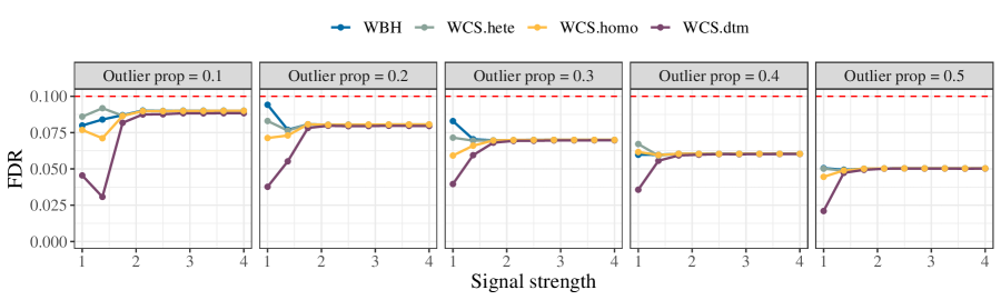
Figure 11: Empirical FDR averaged over $N=1000$ runs under increasing levels $a$ of signal strength. Each subplot corresponds to one value of $\rho_{\texttt{pop}}$. The red dashed lines are at the nominal level $q=0.1$.

Figure 12 plots the power of the four methods. Interestingly, although they differ in FDR, especially when the signal strength is small, they achieve nearly identical power, finding about the same number of true discoveries.

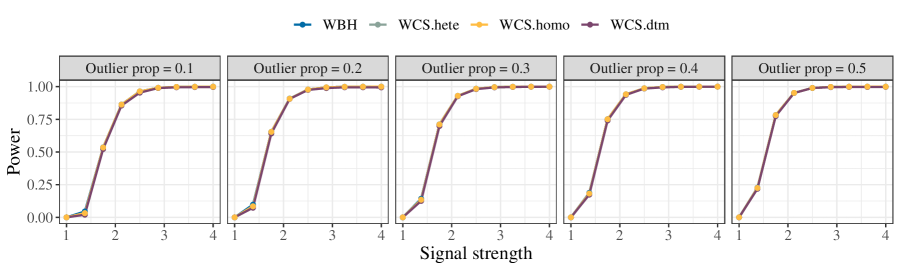
Figure 12: Empirical power averaged over $N=1000$ runs. Everything else is as in Figure 11.

6.3 Real data application

We then apply Algorithm 2 to a bank marketing dataset [MCR14]; this dataset has been used to benchmark outlier detection algorithms [PSvdH19, PSCH21]. In short, each sample in the dataset represents a phone contact to a potential client, whose demographic information such as age, gender, and marital status is also recorded in the features. The outcome is a binary indicator $Y$, where $Y=1$ represents a successful compaign. Positive samples are relatively rare, accounting for about $10\%$ of all records.

In our experiments, we always use negative samples as the calibration data. We find this dataset interesting because the classification and outlier detection perspectives are somewhat blurred here. Viewing this as a classification task, Example 6.2 becomes relevant, and our theory implies FDR control as long as the distribution of negative samples (i.e., that of $X$ given $Y=0$) admits the covariate shift. In the sense of finding positive responses (so as to reach out to these promising clients), controlling the FDR ensures efficient use of campaign resources. Alternatively, from an outlier detection perspective, those $Y=1$ are outliers [PSvdH19] that deserve more attention. Taking either of the two perspectives leads to the same calibration set and the same guarantees following Section 6.1. Perhaps the only methodological distinction is whether positive samples are leveraged in the training process. Similar considerations also appeared in [LSS22], but the scenario therein is more sophisticated than ours as they also use known outliers (positive samples) in constructing p-values. As a classification problem, we may use positive samples to train a classifier and produce nonconformity scores. As an outlier detection problem, however, the widely-used one-class classification relies exclusively on inliers (negative samples). We will evaluate the performance of both (i.e., train the nonconformity score with or without positive samples); see procedures cond_class and outlier below.

For comparison, we additionally evaluate Algorithm 1 which operates under a covariate shift assumption on the joint distribution of $(X,Y)$ (see procedure sup_class below); this is in contrast to Algorithm 2 which puts no assumption on positive samples.

The total sample size is $N=41188$ with $4640$ positive samples. We use rejection sampling to create the covariate shift between training/calibration and test samples. In details, we use a subset of features $X^{*}\in\mathbb{R}^{4}$ representing age and indicators of marriage, basic four-year education, and housing. We first randomly select a subset of the original dataset as the test data. Each sample enters the test data with probability $e(x):=0.125\,\sigma({\theta^{\top}x^{*}})$, where $\theta=(1,1/2,1/2,1/2)^{\top}$. This creates a covariate shift $w(x)\propto e(x)/(1-e(x))$ between null samples in calibration and test folds, so that the test set contains more senior, married, well-educated and housed people.

To test the two perspectives, we consider three procedures with FDR levels $q\in\{0.2,0.5,0.8\}$:

1. sup_class: We randomly split the data that is not in the test fold into two equally-sized halves as the training and calibration folds, $\mathcal{D}_{\textnormal{train}}$ and $\mathcal{D}_{\textnormal{calib}}$. We use $\mathcal{D}_{\textnormal{train}}$ to train an SVM classifier using the scikit-learn Python library with rbf kernel. Then, we apply Algorithm 1 with $V(x,y)=100\cdot y-\widehat{\mu}(x)$, where $\widehat{\mu}(\cdot)$ is the class probability output from the SVM classifier.

2. cond_class: With the same random split as in (i), the first half is used as $\mathcal{D}_{\textnormal{train}}$, while we set $\mathcal{D}_{\textnormal{calib}}$ as the set of negative samples in the second half. We use $\mathcal{D}_{\textnormal{train}}$ to train an SVM classifier in the same way as in (i) to obtain the predicted class probability $\widehat{\mu}(\cdot)$. Lastly, we apply Algorithm 2 with $V(x)=-\widehat{\mu}(x)$.

3. outlier: With the same split, we set $\mathcal{D}_{\textnormal{train}}$ and $\mathcal{D}_{\textnormal{calib}}$ as the two folds after discarding all the negative samples. We use $\mathcal{D}_{\textnormal{train}}$ to train a one-class SVM classifier using the scikit-learn Python library with rbf kernel and obtain the output $\widehat{\mu}(\cdot)$. We then apply Algorithm 2 with $V(x)=-\widehat{\mu}(x)$.

To ensure consistency, in all procedures, the SVM-based classifier uses the parameter gamma$=0.01$. FDPs and power (proportions of true discoveries) across $N=1000$ independent runs are shown in Figures 13 and 14, respectively.

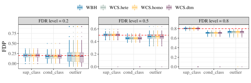
Figure 13: FDPs over $N=1000$ independent data splits. Each subplot corresponds to one nominal FDR level shown by means of red dashed lines.

In Figure 13, we observe FDR control for all the methods in all settings. Across the four testing methods, the FDPs are very similar, hence all of them are reasonable choices. However, both the values and the variability of the FDP vary across settings. The methods cond_class and outlier from Algorithm 2 do not use all of the error budget—note the $\pi_{0}$ factor in Theorem 6.5. In contrast, Algorithm 1 leverages super-population structure (which is present in this problem) and leads to tight FDPs and FDR around the target level. In all cases, the outlier detection approach, where only negative samples are used in the training process, has more variable FDPs. With this dataset, the variability of FDP around the FDR is visible for $q=0.2$, but it decreases as we increase the FDR level.

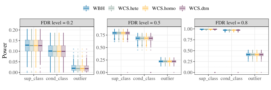
Figure 14: Proportion of true discoveries (empirical power). Everything else is as in Figure 13.

In Figure 14, the power across the four multiple testing methods is similar. However, we observe drastic differences among the three settings. While using the same classifier, cond_class has lower power than sup_class, per our discussion in Section 6.1.3. We also see that outlier has much lower power, which may be due to the fact that the nonconformity score is not sufficiently powerful in distinguishing inliers from outliers as the training process does not use outliers. Our results suggest that in outlier detection problems, even when we do not want to impose any distributional assumption on outliers (so that Algorithm 1 becomes less reasonable), utilizing known outliers may be helpful in obtaining better nonconformity scores.

Finally, we observe negligible difference between the rejection sets returned by the BH procedure and Algorithm 1. There at most five distinct decisions among $\approx 3700$ test samples.

Appendix A Deferred results and details

A.1 Recap: Conformalied Selection

In this section, we briefly recall the conformalized selection framework of [JC22]. As before, set $\mathcal{D}_{\textnormal{calib}}=\{1,\dots,n\}$ and $\mathcal{D}_{\textnormal{test}}=\{n+1,\dots,n+m\}$. Screening for large outcomes can be viewed as testing the null hypotheses

$$H_{j}\colon Y_{n+j}\leq c_{n+j},\quad j=1,\dots,m,$$

where selecting $j\in\mathcal{R}$ is equivalent to rejecting $H_{j}$. Perhaps unconventionally, whether $H_{j}$ is true or not is here a random event. Yet, we still construct conformal p-values built upon the (split) conformal inference framework [VGS05] to test these hypotheses.

Given a monotone score $V$ and thresholds $\{c_{n+j}\}_{j=1}^{m}$, we compute $V_{i}=V(X_{i},Y_{i})$ for $i\in\mathcal{D}_{\textnormal{calib}}$, $\widehat{V}_{n+j}=V(X_{n+j},c_{n+j})$, and then apply the Benjamini-Hochberg (BH) procedure [BH95] to conformal p-values

$$p_{j}^{\textnormal{nw}}=\frac{\sum_{i=1}^{n}\operatorname{\mathds{1}}{\{V_{i}<\widehat{V}_{n+j}\}}+U_{j}(1+\sum_{i=1}^{n}\operatorname{\mathds{1}}{\{V_{i}=\widehat{V}_{n+j}\}})}{n+1},\quad U_{j}\stackrel{{\scriptstyle\textnormal{i.i.d.}}}{{\sim}}\textrm{Unif}([0,1]).$$ (14)

Under the assumption that $Q=P$, or $w(x)\equiv 1$ in (1), each $p_{j}^{\textnormal{nw}}$ is a valid p-value obeying (3). However, as shown earlier, under non-trivial covariate shift, the random variables $p_{j}^{\textnormal{nw}}$ are no longer valid p-values.

A.2 Connection of our p-values and weighted conformal prediction

Remark A.1.

An intuitive interpretation for the p-values in (4) is that they are roughly the critical confidence level when inverting weighted conformal prediction intervals at the thresholds $\{c_{n+j}\}$. Indeed, the split weighted conformal inference procedure [TFBCR19] (using $-V$ as the nonconformity score for consistency) yields the one-sided prediction interval $\widehat{C}(X_{n+j},1-\alpha)=[\eta(X_{n+j},1-\alpha),+\infty)$ for $Y_{n+j}$, where

$$-\eta(x,1-\alpha)=\textrm{Quantile}\big{(}1-\alpha;{\textstyle\sum_{i=1}^{n}}w_{i}(x)\delta_{-V_{i}}+w_{n+1}(x)\delta_{-\infty}\big{)},$$

and $w_{i}(x)=\frac{w(X_{i})}{\sum_{i=1}^{n}w(X_{i})+w(x)}$, $i=1,\dots,n$, and $w_{n+1}(x)=\frac{w(x)}{\sum_{i=1}^{n}w(X_{i})+w(x)}$ for any $x\in\mathcal{X}$. Ignoring the tie-breaking random variables, we see that $p_{j}$ is the smallest $\alpha$ such that $c_{n+j}<\eta(X_{n+j},1-\alpha)$.

A.3 Weighted FDR control for unweighted p-values

The following theorem shows the weighted FDR control when running BH($q$) with unweighted conformal p-values while there is a covariate shift between calibration and test samples.

Theorem A.2.

Suppose $V$ is monotone, $\{(X_{i},Y_{i})\}_{i=1}^{n}\sim P$ and $\{(X_{n+j},Y_{n+j})\}_{j=1}^{m}\sim Q$ are mutually independent and obey (1). Suppose $\{(X_{i},Y_{i})\}_{i=1}^{n}\cup\{(X_{n+\ell},c_{\ell})\}_{\ell\neq j}\cup\{(X_{n+j},Y_{n+j})\}$ are mutually independent for all $j$. For any $q\in(0,1)$, let $\mathcal{R}_{\textnormal{nw}}$ be the rejection set of BH($q$) procedure applied to the unweighted conformal $p$-values $\{p_{j}^{\textnormal{nw}}\}$ in (14). Then

$$\mathbb{E}\Bigg{[}\frac{\sum_{j=1}^{m}\operatorname{\mathds{1}}\{j\in\mathcal{R}_{\textnormal{nw}},Y_{n+j}\leq c_{n+j}\}/w(X_{n+j})}{1\vee|\mathcal{R}_{\textnormal{nw}}|}\Bigg{]}\leq q\cdot\mathbb{E}\bigg{[}\frac{n+1}{\sum_{i=1}^{n}w(X_{i})+w(X_{n+1})}\bigg{]},$$

where the expectation is over both the test and calibration data.

A.4 General theorem for asymptotic FDR control with BH procedure

We provide the general results for Theorem 2.5 below.

Theorem A.3.

Suppose $w(\cdot)$ is uniformly bounded by a fixed constant, the covariate shift (1) holds, and $\{c_{n+j}\}_{j=1}^{m}$ are i.i.d. random variables. Fix any $q\in(0,1)$, and let $\mathcal{R}$ be the output of the BH($q$) procedure applied to $\{p_{j}\}_{j=1}^{m}$ in (4). Then the following two results hold.

1. For any fixed $m$, as $n\to\infty$, it holds that $\limsup_{n\to\infty}\textnormal{FDR}\leq q$.

2. As $m,n\to\infty$, it holds that $\limsup_{m,n\to\infty}\textnormal{FDR}\leq q$ if there exists some $t^{\prime}\in(0,1]$ such that $G_{\infty}(t^{\prime})<q$, where $G_{\infty}(t):=t/\mathbb{P}(F(V(X_{n+j},C_{n+j}),U_{j})\leq t)$ for any $t\in[0,1]$, with the convention that $0/0=0$ and $t/0=\infty$ for $t>0$. Here, for any $v\in\mathbb{R}$ and $u\in[0,1]$,

   $$F(v,u)=Q\big{(}V(X,Y)<v\big{)}+u\cdot Q\big{(}V(X,Y)=v\big{)},$$ (15)

   where the probability is taken with respect to the test distribution $(X,Y)\sim Q$ obeying (1).

   Furthermore, define $t^{*}=\sup\{t\in[0,1]\colon G_{\infty}(t)\leq q\}$. Additionally suppose for any sufficiently small $\epsilon>0$, there exists some $t\in(t^{*}-\epsilon,t)$ such that $G_{\infty}(t)<q$. Then the asymptotic FDR of BH($q$) is $\frac{Q\{F(V(X,C),U)\leq t^{*},Y\leq C\}}{Q\{F(V(X,C),U)\leq t^{*}\}}$, and the asymptotic power is $Q\big{\{}F(V(X,C),U)\leq t^{*}{\,|\,}Y>C\big{\}}$, where all the probabilities are induced by the test distribution $Q_{X,Y,C}$ and an independent $U\sim$ Unif([0,1]).

A.5 Deferred simulation results for DTI prediction

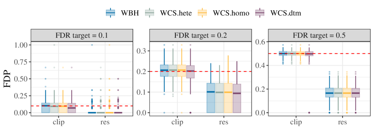
Figure 15: Empirical FDR for DTI prediction with $q_{\textrm{pop}}=0.7$. Details are the same as Figure 4.

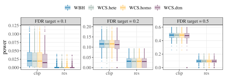
Figure 16: Empirical power for DTI with $q_{\textrm{pop}}=0.7$. Details are the same as Figure 4.

Appendix B Proofs for weighted p-values

B.1 Proof of Lemma 2.2

Proof of Lemma 2.2.

For any $j\in\{1,\dots,m\}$, note that $V(X_{n+j},y)$ is increasing in $y$, thus on the event $\{Y_{n+j}\leq c_{n+j}\}$, it holds that $V_{n+j}\leq\widehat{V}_{n+j}$. We now define

$$p_{j}^{*}=\frac{\sum_{i=1}^{n}w(X_{i})\operatorname{\mathds{1}}{\{V_{i}<{V}_{n+j}\}}+(w(X_{n+j})+\sum_{i=1}^{n}w(X_{i})\operatorname{\mathds{1}}{\{V_{i}={V}_{n+j}\}})\cdot U_{j}}{\sum_{i=1}^{n}w(X_{i})+w(X_{n+j})},$$

where $U_{j}$ is the same tie-breaking random variable as in $p_{j}$. That is, $p_{j}^{*}$ is the oracle p-value we would get if we replace $\widehat{V}_{n+j}$ by $V_{n+j}$ in the construction of $p_{j}$. Note that $p_{j}^{*}$ is not computable; it is only for the purpose of proof. Thus, it is clear that $p_{j}^{*}\leq p_{j}$ on the event $\{Y_{n+j}\leq c_{n+j}\}$. This implies

$$\mathbb{P}(p_{j}\leq t,~{}Y_{n+j}\leq c_{n+j})\leq\mathbb{P}(p_{j}\leq t,~{}p_{j}^{*}\leq p_{j})\leq\mathbb{P}(p_{j}^{*}\leq t).$$

The right-handed side above is below $t$ using weighted exchangeability introduced in [TFBCR19]. Formally, define the unordered set $Z=[Z_{1},\dots,Z_{n},Z_{n+j}]$ for $Z_{i}=(X_{i},Y_{i})$, $i=1,\dots,n,n+j$, and write $z$ as the realized value of $Z$, and $\mathcal{E}_{z}=\{Z=z\}$. Under the covariate shift (1), the scores $\{V_{1},\dots,V_{n},V_{n+j}\}$ are weighted exchangeable, in the sense that

$$Z_{n+j}{\,|\,}\mathcal{E}_{z}~{}\sim~{}\sum_{i\in\{1,\dots,n,n+j\}}\delta_{z_{i}}\cdot\frac{w(x_{i})}{\sum_{i=1}^{n}w(x_{i})+w(x_{n+j})},$$

i.e., given that the unordered set $Z$ equals $z$, the probability that $Z_{n+j}$ taking on any value $(x,y)\in\{z_{1},\dots,z_{n},z_{n+j}\}$ is proportional to the corresponding weight $w(x)$. This implies

$$\mathbb{P}(p_{j}^{*}\leq t{\,|\,}\mathcal{E}_{z})=t,$$

and thus $\mathbb{P}(p_{j}^{*}\leq t)=t$, which concludes the proof of Lemma 2.2. ∎

B.2 Proof of Theorem A.2

Proof of Theorem A.2.

For ease of illustration, we prove the result when there is no tie among all nonconformity scores; similar results can be obtained with ties. We first use a leave-one-out trick similar to [JC22]. Define the oracle conformal p-values

$$\bar{p}_{j}^{\textnormal{nw}}=\frac{\sum_{i=1}^{n}\operatorname{\mathds{1}}{\{V_{i}<{V}_{n+j}\}}+U_{j}(1+\sum_{i=1}^{n}\operatorname{\mathds{1}}{\{V_{i}={V}_{n+j}\}})}{n+1},$$

which is obtained by replacing the $\widehat{V}_{n+j}$ in (14) by $V_{n+j}=V(X_{n+j},Y_{n+j})$. By the monotonicity of $V$, one has $p_{j}^{\textnormal{nw}}\geq\bar{p}_{j}^{\textnormal{nw}}$ for any $j$ such that $Y_{n+j}\leq c_{j}$. In the BH procedure, for any $j\in\mathcal{R}_{\textnormal{nw}}$, replacing $p_{j}$ with a smaller value does not change the rejection set. Therefore, letting $\bar{\mathcal{R}}_{j}$ be the rejection set of BH($q$) applied to $\{p_{1}^{\textnormal{nw}},\dots,p_{j-1}^{\textnormal{nw}},\bar{p}_{j}^{\textnormal{nw}},\dots,p_{m}^{\textnormal{nw}}\}$, we know that

$$j\in\mathcal{R}_{\textnormal{nw}}~{}\textrm{and}~{}Y_{n+j}\leq c_{n+j}\quad\Rightarrow\quad j\in\bar{\mathcal{R}}_{j}~{}\textrm{and}~{}\bar{\mathcal{R}}_{j}=\mathcal{R}_{\textnormal{nw}}.$$

We then have

$$\mathbb{E}\Bigg{[}\frac{\sum_{j=1}^{m}\operatorname{\mathds{1}}\{j\in\mathcal{R}_{\textnormal{nw}},Y_{n+j}\leq c_{n+j}\}/w(X_{n+j})}{1\vee|\mathcal{R}_{\textnormal{nw}}|}\Bigg{]}\leq\sum_{j=1}^{m}\mathbb{E}\Bigg{[}\frac{\operatorname{\mathds{1}}\{j\in\bar{\mathcal{R}}_{j}\}/w(X_{n+j})}{1\vee|\bar{\mathcal{R}}_{j}|}\Bigg{]}.$$ (16)

Also note that $j\in\bar{\mathcal{R}}_{j}$ if and only if $\bar{p}_{j}^{\textnormal{nw}}\leq q|\bar{\mathcal{R}}_{j}|/m$. Thus, for any $j=1,\dots,m$,

$$\mathbb{E}\Bigg{[}\frac{\operatorname{\mathds{1}}\{j\in\bar{\mathcal{R}}_{j}\}/w(X_{n+j})}{1\vee|\bar{\mathcal{R}}_{j}|}\Bigg{]}=\sum_{k=1}^{m}\frac{1}{k}\mathbb{E}\big{[}\operatorname{\mathds{1}}{\{|\bar{\mathcal{R}}_{j}|=k\}}\operatorname{\mathds{1}}{\{\bar{p}_{j}^{\textnormal{nw}}\leq qk/m\}}/w(X_{n+j})\big{]}$$

$$=\sum_{k=1}^{m}\frac{1}{k}\mathbb{E}\big{[}(\operatorname{\mathds{1}}{\{|\bar{\mathcal{R}}_{j}|\leq k\}}-\operatorname{\mathds{1}}{\{|\bar{\mathcal{R}}_{j}|\leq k-1\}})\cdot\operatorname{\mathds{1}}{\{\bar{p}_{j}^{\textnormal{nw}}\leq qk/m\}}/w(X_{n+j})\big{]}$$

$$\leq\frac{1}{m}\mathbb{E}\bigg{[}\frac{\operatorname{\mathds{1}}{\{\bar{p}_{j}^{\textnormal{nw}}\leq q\}}}{w(X_{n+j})}\bigg{]}+\sum_{k=1}^{m-1}\mathbb{E}\bigg{[}\frac{\operatorname{\mathds{1}}{\{|\bar{\mathcal{R}}_{j}|\leq k\}}\operatorname{\mathds{1}}{\{\bar{p}_{j}^{\textnormal{nw}}\leq\frac{qk}{m}\}}}{k\cdot w(X_{n+j})}-\frac{\operatorname{\mathds{1}}{\{|\bar{\mathcal{R}}_{j}|\leq k\}}\operatorname{\mathds{1}}{\{\bar{p}_{j}^{\textnormal{nw}}\leq\frac{q(k+1)}{m}\}}}{(k+1)\cdot w(X_{n+j})}\bigg{]}.$$ (17)

We define the event $\mathcal{E}_{z}=\{Z=z\}$, where $Z=[Z_{1},\dots,Z_{n},Z_{n+j}]$ is the unordered set for $Z_{i}=(X_{i},Y_{i})$ and $Z_{n+j}=(X_{n+j},Y_{n+j})$, and $z=[z_{1},\dots,z_{n},z_{n+j}]$ is the unordered set of their realized values. By the covariate shift (1), $\{(X_{i},Y_{i})\}_{i=1}^{n}$ and $(X_{n+j},Y_{n+j})$ are weighted exchangeable [TFBCR19], hence

$$Z_{n+j}{\,|\,}\mathcal{E}_{z}~{}\sim~{}\sum_{i\in\{1,\dots,n,n+j\}}\delta_{z_{i}}\cdot\frac{w(x_{i})}{\sum_{i=1}^{n}w(x_{i})+w(x_{n+j})},$$ (18)

where $\delta_{z_{i}}$ is the point mass on $z_{i}$. Therefore, by the tower property,

$$\mathbb{E}\Bigg{[}\frac{\operatorname{\mathds{1}}{\{|\bar{\mathcal{R}}_{j}|\leq k\}}\operatorname{\mathds{1}}{\{\bar{p}_{j}^{\textnormal{nw}}\leq qk/m\}}}{k\cdot w(X_{n+j})}-\frac{\operatorname{\mathds{1}}{\{|\bar{\mathcal{R}}_{j}|\leq k\}}\operatorname{\mathds{1}}{\{\bar{p}_{j}^{\textnormal{nw}}\leq q(k+1)/m\}}}{(k+1)\cdot w(X_{n+j})}\,\bigg{|}\,\mathcal{E}_{z}\Bigg{]}$$

$$\leq\mathbb{E}\Bigg{[}\frac{\operatorname{\mathds{1}}{\{\bar{p}_{j}^{\textnormal{nw}}\leq qk/m\}}}{w(X_{n+j})}\cdot\frac{1}{k}\cdot\mathbb{P}\big{(}|\bar{\mathcal{R}}_{j}|\leq k\,\big{|}\,\bar{p}_{j}^{\textnormal{nw}},\mathcal{E}_{z}\big{)}\,\bigg{|}\,\mathcal{E}_{z}\Bigg{]}$$

$$\quad-\mathbb{E}\Bigg{[}\frac{\operatorname{\mathds{1}}{\{\bar{p}_{j}^{\textnormal{nw}}\leq q(k+1)/m\}}}{w(X_{n+j})}\cdot\frac{1}{k+1}\cdot\mathbb{P}\big{(}|\bar{\mathcal{R}}_{j}|\leq k\,\big{|}\,\bar{p}_{j}^{\textnormal{nw}},\mathcal{E}_{z}\big{)}\,\bigg{|}\,\mathcal{E}_{z}\Bigg{]}$$

Note that the randomness in $U_{j}$ is independent of everything else, hence conditioning on $(\bar{p}_{j}^{\textnormal{nw}},\mathcal{E}_{z})$ is the same as conditioning on $(Z_{n+j},\mathcal{E}_{z})$. We also denote $[1],[2],\dots,[n+1]$ as a permutation of $(1,2,\dots,n,n+j)$ such that $V(X_{[1]},Y_{[1]})\leq V(X_{[2]},Y_{[2]})\leq\cdots\leq V(X_{[n+1]},Y_{[n+1]})$. Conditional on $\mathcal{E}_{z}$, on the event $\{\bar{p}_{j}^{\textnormal{nw}}\leq qk/m\}$, $Z_{n+j}$ can only take values at $z_{i}$ for which $\frac{\sum_{\ell\neq i}\operatorname{\mathds{1}}{\{V(z_{\ell})<V(z_{k})\}}}{n+1}\leq qk/m$; that is, the possible values of $Z_{n+j}$ are in the ordered set $\{z_{[1]},\dots,z_{[i_{k}]}\}$ for some $i_{k}$. Similarly, $Z_{n+j}$ can only take values in $\{z_{[1]},\dots,z_{[i_{k+1}]}\}$ for $i_{k+1}\geq i_{k}$ on the event $\{\bar{p}_{j}^{\textnormal{nw}}\leq q(k+1)/m\}$. Therefore, we have

$$\mathbb{E}\Bigg{[}\frac{\operatorname{\mathds{1}}{\{|\bar{\mathcal{R}}_{j}|\leq k\}}\operatorname{\mathds{1}}{\{\bar{p}_{j}^{\textnormal{nw}}\leq qk/m\}}}{k\cdot w(X_{n+j})}-\frac{\operatorname{\mathds{1}}{\{|\bar{\mathcal{R}}_{j}|\leq k\}}\operatorname{\mathds{1}}{\{\bar{p}_{j}^{\textnormal{nw}}\leq q(k+1)/m\}}}{(k+1)\cdot w(X_{n+j})}\,\bigg{|}\,\mathcal{E}_{z}\Bigg{]}$$

$$\leq\mathbb{E}\Bigg{[}\sum_{\ell=1}^{i_{k}}\operatorname{\mathds{1}}{\{Z_{n+j}=z_{[\ell]}\}}\frac{\operatorname{\mathds{1}}{\{\bar{p}_{j}^{\textnormal{nw}}\leq qk/m\}}}{w(x_{[\ell]})}\cdot\frac{1}{k}\cdot\mathbb{P}\big{(}|\bar{\mathcal{R}}_{j}|\leq k\,\big{|}\,Z_{n+j}=z_{[\ell]},\mathcal{E}_{z}\big{)}\,\bigg{|}\,\mathcal{E}_{z}\Bigg{]}$$

$$\quad-\mathbb{E}\Bigg{[}\sum_{\ell=1}^{i_{k+1}}\operatorname{\mathds{1}}{\{Z_{n+j}=z_{[\ell]}\}}\frac{\operatorname{\mathds{1}}{\{\bar{p}_{j}^{\textnormal{nw}}\leq q(k+1)/m\}}}{w(x_{[\ell]})}\cdot\frac{1}{k+1}\cdot\mathbb{P}\big{(}|\bar{\mathcal{R}}_{j}|\leq k\,\big{|}\,Z_{n+j}=z_{[\ell]},\mathcal{E}_{z}\big{)}\,\bigg{|}\,\mathcal{E}_{z}\Bigg{]}$$

$$=\sum_{\ell=1}^{i_{k}}\frac{\mathbb{P}\big{(}|\bar{\mathcal{R}}_{j}|\leq k\,\big{|}\,Z_{n+j}=z_{[\ell]},\mathcal{E}_{z}\big{)}}{k\cdot w(x_{[\ell]})}\mathbb{E}\big{[}\operatorname{\mathds{1}}{\{Z_{n+j}=z_{[\ell]}\}}\operatorname{\mathds{1}}{\{\bar{p}_{j}^{\textnormal{nw}}\leq qk/m\}}\,\big{|}\,\mathcal{E}_{z}\big{]}$$

$$\quad-\sum_{\ell=1}^{i_{k+1}}\frac{\mathbb{P}\big{(}|\bar{\mathcal{R}}_{j}|\leq k\,\big{|}\,Z_{n+j}=z_{[\ell]},\mathcal{E}_{z}\big{)}}{(k+1)\cdot w(x_{[\ell]})}\mathbb{E}\big{[}\operatorname{\mathds{1}}{\{Z_{n+j}=z_{[\ell]}\}}\operatorname{\mathds{1}}{\{\bar{p}_{j}^{\textnormal{nw}}\leq q(k+1)/m\}}\,\big{|}\,\mathcal{E}_{z}\big{]}.$$

By weighted exchangeability, for $i<i_{k}$ it holds deterministically that $\bar{p}_{j}^{\textnormal{nw}}\leq qk/m$ and $\mathbb{P}(Z_{n+j}=z_{[\ell]}{\,|\,}\mathcal{E}_{z})=\frac{w(x_{[\ell]})}{\sum_{i=1}^{n}w(x_{i})+w(x_{n+j})}$. The randomness of $U_{j}\sim\textrm{Unif}(0,1)$ implies

$$\mathbb{E}\big{[}\operatorname{\mathds{1}}{\{Z_{n+j}=z_{[i_{k}]}\}}\operatorname{\mathds{1}}{\{\bar{p}_{j}^{\textnormal{nw}}\leq qk/m\}}\,\big{|}\,\mathcal{E}_{z}\big{]}=(n+1)\cdot\bigg{(}\frac{qk}{m}-\frac{i_{k}-1}{n+1}\bigg{)}\cdot\frac{x_{[i_{k}]}}{\sum_{i=1}^{n}w(x_{i})+w(x_{n+j})}.$$

As a result, we have

$$\sum_{\ell=1}^{i_{k}}\frac{\mathbb{P}\big{(}|\bar{\mathcal{R}}_{j}|\leq k\,\big{|}\,Z_{n+j}=z_{[\ell]},\mathcal{E}_{z}\big{)}}{k\cdot w(x_{[\ell]})}\mathbb{E}\big{[}\operatorname{\mathds{1}}{\{Z_{n+j}=z_{[\ell]}\}}\operatorname{\mathds{1}}{\{\bar{p}_{j}^{\textnormal{nw}}\leq qk/m\}}\,\big{|}\,\mathcal{E}_{z}\big{]}$$

$$=\sum_{\ell=1}^{i_{k}-1}\frac{\mathbb{P}\big{(}|\bar{\mathcal{R}}_{j}|\leq k\,\big{|}\,Z_{n+j}=z_{[\ell]},\mathcal{E}_{z}\big{)}}{k\cdot(\sum_{i=1}^{n}w(x_{i})+w(x_{n+j}))}+\frac{(n+1)\frac{qk}{m}-i_{k}+1}{k\cdot(\sum_{i=1}^{n}w(x_{i})+w(x_{n+j}))}\cdot\mathbb{P}\big{(}|\bar{\mathcal{R}}_{j}|\leq k\,\big{|}\,Z_{n+j}=z_{[i_{k}]},\mathcal{E}_{z}\big{)}.$$

Similar computation for $k+1$ leads to

$$\mathbb{E}\Bigg{[}\frac{\operatorname{\mathds{1}}{\{|\bar{\mathcal{R}}_{j}|\leq k\}}\operatorname{\mathds{1}}{\{\bar{p}_{j}^{\textnormal{nw}}\leq qk/m\}}}{k\cdot w(X_{n+j})}-\frac{\operatorname{\mathds{1}}{\{|\bar{\mathcal{R}}_{j}|\leq k\}}\operatorname{\mathds{1}}{\{\bar{p}_{j}^{\textnormal{nw}}\leq q(k+1)/m\}}}{(k+1)\cdot w(X_{n+j})}\,\bigg{|}\,\mathcal{E}_{z}\Bigg{]}$$

$$\leq\sum_{\ell=1}^{i_{k}-1}\frac{\mathbb{P}\big{(}|\bar{\mathcal{R}}_{j}|\leq k\,\big{|}\,Z_{n+j}=z_{[\ell]},\mathcal{E}_{z}\big{)}}{k\cdot(\sum_{i=1}^{n}w(x_{i})+w(x_{n+j}))}-\sum_{\ell=1}^{i_{k+1}-1}\frac{\mathbb{P}\big{(}|\bar{\mathcal{R}}_{j}|\leq k\,\big{|}\,Z_{n+j}=z_{[\ell]},\mathcal{E}_{z}\big{)}}{(k+1)\cdot(\sum_{i=1}^{n}w(x_{i})+w(x_{n+j}))}$$

$$\quad-\frac{(n+1)\frac{qk}{m}-i_{k}+1}{k\cdot(\sum_{i=1}^{n}w(x_{i})+w(x_{n+j}))}\cdot\mathbb{P}\big{(}|\bar{\mathcal{R}}_{j}|\leq k\,\big{|}\,Z_{n+j}=z_{[i_{k}]},\mathcal{E}_{z}\big{)}$$

$$\quad-\frac{(n+1)\frac{q(k+1)}{m}-i_{k+1}+1}{(k+1)\cdot(\sum_{i=1}^{n}w(x_{i})+w(x_{n+j}))}\cdot\mathbb{P}\big{(}|\bar{\mathcal{R}}_{j}|\leq k\,\big{|}\,Z_{n+j}=z_{[i_{k+1}]},\mathcal{E}_{z}\big{)}.$$

Conditional on $\mathcal{E}_{z}$, $\mathbb{P}\big{(}|\bar{\mathcal{R}}_{j}|\leq k\,\big{|}\,Z_{n+j}=z_{[\ell]},\mathcal{E}_{z}\big{)}$ is increasing in $\ell$; to see this, simply note that the p-values $(p_{1}^{\textnormal{nw}},\dots,p_{j-1}^{\textnormal{nw}},\bar{p}_{j}^{\textnormal{nw}},p_{j+1}^{\textnormal{nw}},\dots,p_{m}^{\textnormal{nw}})$ are coordinate-wisely increasing in $\ell$, hence the size of the rejection set $\bar{\mathcal{R}}_{j}$ is decreasing in $\ell$. Thus, replacing the index $\ell$ in the two summations by $i_{k}$, we have

$$\mathbb{E}\Bigg{[}\frac{\operatorname{\mathds{1}}{\{|\bar{\mathcal{R}}_{j}|\leq k\}}\operatorname{\mathds{1}}_{\{p_{j}^{*}\leq qk/m\}}}{k\cdot w(X_{n+j})}-\frac{\operatorname{\mathds{1}}_{\{|\bar{\mathcal{R}}_{j}|\leq k\}}\operatorname{\mathds{1}}_{\{p_{j}^{*}\leq q(k+1)/m\}}}{(k+1)\cdot w(X_{n+j})}\,\bigg{|}\,\mathcal{E}_{z}\Bigg{]}$$

$$\leq\sum_{\ell=1}^{i_{k}-1}\frac{\mathbb{P}\big{(}|\bar{\mathcal{R}}_{j}|\leq k\,\big{|}\,Z_{n+j}=z_{[i_{k}]},\mathcal{E}_{z}\big{)}}{k\cdot(\sum_{i=1}^{n}w(x_{i})+w(x_{n+j}))}-\sum_{\ell=1}^{i_{k+1}-1}\frac{\mathbb{P}\big{(}|\bar{\mathcal{R}}_{j}|\leq k\,\big{|}\,Z_{n+j}=z_{[i_{k}]},\mathcal{E}_{z}\big{)}}{(k+1)\cdot(\sum_{i=1}^{n}w(x_{i})+w(x_{n+j}))}$$

$$\quad+\frac{(n+1)\frac{qk}{m}-i_{k}+1}{k\cdot(\sum_{i=1}^{n}w(x_{i})+w(x_{n+j}))}\mathbb{P}\big{(}|\bar{\mathcal{R}}_{j}|\leq k\,\big{|}\,Z_{n+j}=z_{[i_{k}]},\mathcal{E}_{z}\big{)}$$

$$\quad+\frac{(n+1)\frac{q(k+1)}{m}-i_{k+1}+1}{(k+1)\cdot(\sum_{i=1}^{n}w(x_{i})+w(x_{n+j}))}\mathbb{P}\big{(}|\bar{\mathcal{R}}_{j}|\leq k\,\big{|}\,Z_{n+j}=z_{[i_{k}]},\mathcal{E}_{z}\big{)}$$

$$=\frac{\mathbb{P}\big{(}|\bar{\mathcal{R}}_{j}|\leq k\,\big{|}\,Z_{n+j}=z_{[i_{k}]},\mathcal{E}_{z}\big{)}}{\sum_{i=1}^{n}w(x_{i})+w(x_{n+j})}\Big{(}\frac{(n+1)qk/m}{k}-\frac{(n+1)q(k+1)/m}{k+1}\Big{)}=0.$$

For any $j$, the first term in (B.2) can be calculated as

$$\mathbb{E}\big{[}\operatorname{\mathds{1}}{\{\bar{p}_{j}^{\textnormal{nw}}\leq q\}}/w(X_{n+j})\,\big{|}\,\mathcal{E}_{z}\big{]} =\sum_{\ell=1}^{i_{m}}\frac{\mathbb{P}(\bar{p}_{j}^{\textnormal{nw}}\leq q{\,|\,}Z_{n+j}=z_{[\ell]},\mathcal{E}_{z})\cdot\mathbb{P}(Z_{n+j}=z_{[\ell]}{\,|\,}\mathcal{E}_{z})}{w(x_{[\ell]})}$$

$$=\frac{i_{m}-1+(n+1)q-i_{m}+1}{\sum_{i=1}^{n}w(x_{i})+w(x_{n+j})}=\frac{(n+1)q}{\sum_{i=1}^{n}w(x_{i})+w(x_{n+j})},$$

where the second equality uses (18), and the definition of $\bar{p}_{j}^{\textnormal{nw}}$. Returning to (16) and (B.2), we obtain

$$\mathbb{E}\Bigg{[}\frac{\sum_{j=1}^{m}\operatorname{\mathds{1}}\{j\in\mathcal{R}_{\textnormal{nw}},Y_{n+j}\leq c_{n+j}\}/w(X_{n+j})}{1\vee|\mathcal{R}^{\textnormal{nw}}|}\Bigg{]}$$

$$\leq\frac{1}{m}\sum_{j=1}^{m}\mathbb{E}\big{[}\operatorname{\mathds{1}}{\{\bar{p}_{j}^{\textnormal{nw}}\leq q\}}/w(X_{n+j})\big{]}=\mathbb{E}\bigg{[}\frac{(n+1)q}{\sum_{i=1}^{n}w(X_{i})+w(X_{n+1})}\bigg{]},$$

where the last equality uses the fact that the covariates of test data are i.i.d. This concludes the proof of Theorem A.2. ∎

B.3 Proof of Non-PRDS

Proof of Proposition 2.4.

Without loss of generality, we consider the oracle p-values

$$p_{j}^{*}=\frac{\sum_{i=1}^{n}w(X_{i})\operatorname{\mathds{1}}{\{V_{i}<{V}_{n+j}\}}+(w(X_{n+j})+\sum_{i=1}^{n}w(X_{i})\operatorname{\mathds{1}}{\{V_{i}={V}_{n+j}\}})\cdot U_{j}}{\sum_{i=1}^{n}w(X_{i})+w(X_{n+j})},$$ (19)

which coincide with (4) when $Y_{n+j}=c_{n+j}$.

We prove by constructing a counterexample and computing the distribution functions of p-values to show the violation of the PRDS property. We set $w(x)=x$ for $P=\textrm{Unif}([1/2,3/2])$, let $Q$ have density function $q(x)=x\operatorname{\mathds{1}}\{1/2\leq x\leq 3/2\}$, and $V(x,y)=-w(x)$. Take $n=2$ and any arbitrary $m\geq 2$. If the weighted conformal p-values are PRDS, we would have

$$F(s,t):=\mathbb{P}(p_{1}\leq s{\,|\,}p_{2}\geq t)$$

is decreasing in $t\in(0,1)$ for any fixed $s\in(0,1)$. However, we will show $F(\frac{1}{10},\frac{3}{5})<F(\frac{1}{10},\frac{9}{10})$. We will compute the two values exactly; they can also be approximated to arbitrary accuracy via Monte Carlo.

For notational simplicity, we write $W_{i}=w(X_{i})$ for $i=1,2$, and $\widetilde{W}_{j}=w(X_{2+j})$ for $j=1,2$. By construction, $W_{1},W_{2},\widetilde{W}_{1},\widetilde{W}_{2}$ are mutually independent with $W_{1},W_{2}\sim P$, $\widetilde{W}_{1},\widetilde{W}_{2}\sim Q$. As $P$ and $Q$ do not have point mass, there are no ties among the four scores almost surely. By the symmetry of $W_{1},W_{2}$, for any $s,t\in(0,1)$, we have

$$F(s,t)=(1-t)^{-1}\cdot\mathbb{P}(p_{1}\leq s,p_{2}\geq t)=2(1-t)^{-1}\cdot\mathbb{P}(p_{1}\leq s,p_{2}\geq t,W_{1}<W_{2}).$$

Since $v(x,y)=-w(x)$, the two weighted conformal p-values are equivalently

$$p_{i}=\frac{W_{1}\operatorname{\mathds{1}}\{W_{1}>\widetilde{W}_{i}\}+W_{2}\operatorname{\mathds{1}}\{W_{2}>\widetilde{W}_{i}\}+U_{i}\widetilde{W}_{i}}{W_{1}+W_{2}+\widetilde{W}_{i}},\quad i=1,2.$$

When $W_{1}<W_{2}$, the form of $p_{i}$ can be divided into three cases:

1. When $\widetilde{W}_{i}<W_{1}<W_{2}$, one has $p_{i}=\frac{W_{1}+W_{2}+U_{i}\widetilde{W}_{i}}{W_{1}+W_{2}+\widetilde{W}_{i}}$, and $p_{i}\in[2/3,1]$ holds deterministically.

2. When $W_{1}<\widetilde{W}_{i}<W_{2}$, one has $p_{i}=\frac{W_{2}+U_{i}\widetilde{W}_{i}}{W_{1}+W_{2}+\widetilde{W}_{i}}$. As $W_{i},\widetilde{W}_{i}\in[1/2,3/2]$, it holds that $p_{i}\in[1/3,6/7]$.

3. When $W_{1}<W_{2}<\widetilde{W}_{i}$, one has $p_{i}=\frac{U_{i}\widetilde{W}_{i}}{W_{1}+W_{2}+\widetilde{W}_{i}}$, and $p_{i}\in[0,3/5]$.

Intuitively, the reason for violating PRDS in this case is that, when $p_{1}\leq 1/10$ is small, it must always take the form $p_{1}=\frac{U_{1}\cdot\widetilde{W}_{1}}{W_{1}+W_{2}+\widetilde{W}_{1}}$ as in case (iii). Meanwhile, when $p_{2}\geq 3/5$ is relatively large, it may be as cases (i) or (ii). In that two cases, roughly, a larger $p_{2}$ means relatively larger $W_{1},W_{2}$, hence smaller $p_{1}$.

We now conduct the exact computation. For $t=9/10$, when $W_{1}<W_{2}$, we note that it must be $p_{2}=\frac{W_{1}+W_{2}+U_{2}\widetilde{W}_{2}}{W_{1}+W_{2}+\widetilde{W}_{2}}$, i.e., $\widetilde{W}_{2}<W_{1}<W_{2}<\widetilde{W}_{1}$. Therefore,

$$\mathbb{P}(p_{1}\leq 1/10,p_{2}\geq 9/10,W_{1}<W_{2})$$

$$=\mathbb{P}\big{(}p_{1}\leq 1/10,p_{2}\geq 9/10,\widetilde{W}_{2}<W_{1}<W_{2}<\widetilde{W}_{1}\big{)}$$

$$=\mathbb{P}\Bigg{(}\frac{U_{1}\cdot\widetilde{W}_{1}}{W_{1}+W_{2}+\widetilde{W}_{1}}\leq\frac{1}{10},~{}\frac{W_{1}+W_{2}+U_{2}\widetilde{W}_{2}}{W_{1}+W_{2}+\widetilde{W}_{2}}\geq\frac{9}{10},~{}\widetilde{W}_{2}<W_{1}<W_{2}<\widetilde{W}_{1}\Bigg{)}$$

$$=\mathbb{P}\Bigg{(}\frac{U_{1}\cdot\widetilde{W}_{1}}{W_{1}+W_{2}+\widetilde{W}_{1}}\leq\frac{1}{10},~{}\frac{W_{1}+W_{2}+U_{2}\widetilde{W}_{2}}{W_{1}+W_{2}+\widetilde{W}_{2}}\geq\frac{9}{10},~{}\widetilde{W}_{2}<W_{1}<W_{2}<\widetilde{W}_{1}\Bigg{)}$$

$$=\mathbb{P}\Bigg{(}U_{1}\leq\frac{W_{1}+W_{2}+\widetilde{W}_{1}}{10\widetilde{W}_{1}},~{}1-U_{2}\geq\frac{W_{1}+W_{2}+\widetilde{W}_{2}}{10\widetilde{W}_{2}},~{}\widetilde{W}_{2}<W_{1}<W_{2}<\widetilde{W}_{1}\Bigg{)}.$$ (20)

We note that in this case $\frac{W_{1}+W_{2}+\widetilde{W}_{1}}{10\widetilde{W}_{1}},\frac{W_{1}+W_{2}+\widetilde{W}_{2}}{10\widetilde{W}_{2}}\in[0,1]$ deterministically. Since $U_{1},U_{2}$ are mutually independent, and also independent of everything else, by the tower property,

$$\eqref{eq:prob1}=\mathbb{E}\Bigg{[}\frac{W_{1}+W_{2}+\widetilde{W}_{1}}{10\widetilde{W}_{1}}\cdot\frac{W_{1}+W_{2}+\widetilde{W}_{2}}{10\widetilde{W}_{2}}\cdot\operatorname{\mathds{1}}\{\widetilde{W}_{2}<W_{1}<W_{2}<\widetilde{W}_{1}\}\Bigg{]}.$$

By the symmetry of $W_{1},W_{2}$, we know

$$\mathbb{P}(p_{1}\leq 1/10,p_{2}\geq 9/10)=2\times\eqref{eq:prob1}$$

$$=\mathbb{E}\Bigg{[}\frac{W_{1}+W_{2}+\widetilde{W}_{1}}{10\widetilde{W}_{1}}\cdot\frac{W_{1}+W_{2}+\widetilde{W}_{2}}{10\widetilde{W}_{2}}\cdot\operatorname{\mathds{1}}\{W_{1},W_{2}\in[\widetilde{W}_{2},\widetilde{W}_{1}],\widetilde{W}_{2}<\widetilde{W}_{1}]\}\Bigg{]}.$$ (21)

Note that conditional on $\widetilde{W}_{2},\widetilde{W}_{1}$ and the event $\{W_{1},W_{2}\in[\widetilde{W}_{2},\widetilde{W}_{1}]\}$, one has $W_{1},W_{2}\sim\textrm{Unif}([\widetilde{W}_{1},\widetilde{W}_{2}])$ and are mutually independent. Applying tower property again, we have

$$\eqref{eq:prob12} =\mathbb{E}\Bigg{[}\frac{13\widetilde{W}_{1}^{2}/6+13\widetilde{W}_{2}^{2}/6+14\widetilde{W}_{1}\widetilde{W}_{2}/3}{100\widetilde{W}_{1}\cdot\widetilde{W}_{2}}\cdot\mathbb{P}\big{(}W_{1},W_{2}\in[\widetilde{W}_{2},\widetilde{W}_{1}]\,\big{|}\,\widetilde{W}_{1},\widetilde{W}_{2}\big{)}\cdot\operatorname{\mathds{1}}\{\widetilde{W}_{2}<\widetilde{W}_{1}\}\Bigg{]}$$

$$=\mathbb{E}\Bigg{[}\frac{13\widetilde{W}_{1}^{2}/6+13\widetilde{W}_{2}^{2}/6+14\widetilde{W}_{1}\widetilde{W}_{2}/3}{100\widetilde{W}_{1}\cdot\widetilde{W}_{2}}\cdot(\widetilde{W}_{1}-\widetilde{W}_{1})^{2}\cdot\operatorname{\mathds{1}}\{\widetilde{W}_{2}<\widetilde{W}_{1}\}\Bigg{]}=\frac{547}{72000},$$

where the exact number can be computed using the distribution of $\widetilde{W}_{1}$ and $\widetilde{W}_{2}$. We thus have

$$F(1/10,9/10)=\frac{547}{7200}.$$

For $t=3/5$, when $p_{2}\geq t$ it could either be case (i) or (ii). Thus

$$\mathbb{P}(p_{1}\leq 1/10,p_{2}\geq 3/5,W_{1}<W_{2}) =\mathbb{P}(p_{1}\leq 1/10,p_{2}\geq 3/5,\widetilde{W}_{2}<W_{1}<W_{2}<\widetilde{W}_{1})$$

$$\qquad+\mathbb{P}(p_{1}\leq 1/10,p_{2}\geq 3/5,W_{1}<\widetilde{W}_{2}<W_{2}<\widetilde{W}_{1}).$$

For the first case,

$$\mathbb{P}(p_{1}\leq 1/10,p_{2}\geq 3/5,\widetilde{W}_{2}<W_{1}<W_{2}<\widetilde{W}_{1})$$

$$=\mathbb{P}\Bigg{(}U_{1}\leq\frac{W_{1}+W_{2}+\widetilde{W}_{1}}{10\widetilde{W}_{1}},~{}1-U_{2}\geq\frac{2W_{1}+2W_{2}+2\widetilde{W}_{2}}{5\widetilde{W}_{2}},~{}\widetilde{W}_{2}<W_{1}<W_{2}<\widetilde{W}_{1}\Bigg{)}.$$ (22)

One can check that $\frac{2W_{1}+2W_{2}+2\widetilde{W}_{2}}{5\widetilde{W}_{2}}\geq\frac{6}{5}$ when $\widetilde{W}_{2}<W_{1}<W_{2}$, and that $\frac{W_{1}+W_{2}+\widetilde{W}_{1}}{10\widetilde{W}_{1}}\in[0,1]$, hence by the tower property and the symmetry of $W_{1},W_{2}$, we know

$$\eqref{eq:prob2} =\mathbb{E}\Bigg{[}\frac{W_{1}+W_{2}+\widetilde{W}_{1}}{10\widetilde{W}_{1}}\cdot\operatorname{\mathds{1}}\{\widetilde{W}_{2}<W_{1}<W_{2}<\widetilde{W}_{1}\}\Bigg{]}$$

$$=\frac{1}{2}\cdot\mathbb{E}\Bigg{[}\mathbb{E}\bigg{[}\frac{W_{1}+W_{2}+\widetilde{W}_{1}}{10\widetilde{W}_{1}}\,\bigg{|}\,W_{1},W_{2}\in[\widetilde{W}_{2},\widetilde{W}_{1}],\widetilde{W}_{1},\widetilde{W}_{2}\bigg{]}\cdot\mathbb{P}\big{(}W_{1},W_{2}\in[\widetilde{W}_{2},\widetilde{W}_{1}]\,\big{|}\,\widetilde{W}_{1},\widetilde{W}_{2}\big{)}\cdot\operatorname{\mathds{1}}\{\widetilde{W}_{2}<\widetilde{W}_{1}\}\Bigg{]}$$

$$=\frac{1}{2}\cdot\mathbb{E}\Bigg{[}\mathbb{E}\bigg{[}\frac{W_{1}+W_{2}+\widetilde{W}_{1}}{10\widetilde{W}_{1}}\,\bigg{|}\,W_{1},W_{2}\in[\widetilde{W}_{2},\widetilde{W}_{1}],\widetilde{W}_{1},\widetilde{W}_{2}\bigg{]}\cdot(\widetilde{W}_{1}-\widetilde{W}_{2})^{2}\cdot\operatorname{\mathds{1}}\{\widetilde{W}_{2}<\widetilde{W}_{1}\}\Bigg{]}$$

Conditional on $\widetilde{W}_{1},\widetilde{W}_{2}$ and the event $\{W_{1},W_{2}\in[\widetilde{W}_{2},\widetilde{W}_{1}]\}$, we know $W_{1},W_{2}\sim\textrm{Unif}([\widetilde{W}_{2},\widetilde{W}_{1}])$, and are mutually independent. Applying the tower property again, we have

$$\eqref{eq:prob2} =\frac{1}{2}\cdot\mathbb{E}\Bigg{[}\frac{2\widetilde{W}_{1}+\widetilde{W}_{2}}{10\widetilde{W}_{1}}\cdot(\widetilde{W}_{1}-\widetilde{W}_{2})^{2}\cdot\operatorname{\mathds{1}}\{\widetilde{W}_{2}<\widetilde{W}_{1}\}\Bigg{]}=\frac{47}{4800}.$$

For the second case,

$$\mathbb{P}(p_{1}\leq 1/10,p_{2}\geq 3/5,W_{1}<\widetilde{W}_{2}<W_{2}<\widetilde{W}_{1})$$

$$=\mathbb{P}\Bigg{(}U_{1}\leq\frac{W_{1}+W_{2}+\widetilde{W}_{1}}{10\widetilde{W}_{1}},~{}1-U_{2}\geq\frac{-3W_{1}+2W_{2}+2\widetilde{W}_{2}}{5\widetilde{W}_{2}},~{}W_{1}<\widetilde{W}_{2}<W_{2}<\widetilde{W}_{1}\Bigg{)}.$$ (23)

One can check that $\frac{W_{1}+W_{2}+\widetilde{W}_{1}}{10\widetilde{W}_{1}},\frac{-3W_{1}+2W_{2}+2\widetilde{W}_{2}}{5\widetilde{W}_{2}}\in[0,1]$. The tower property thus implies

$$\eqref{eq:prob3} =\mathbb{E}\Bigg{[}\frac{W_{1}+W_{2}+\widetilde{W}_{1}}{10\widetilde{W}_{1}}\cdot\frac{-3W_{1}+2W_{2}+2\widetilde{W}_{2}}{5\widetilde{W}_{2}}\cdot\operatorname{\mathds{1}}\{W_{1}<\widetilde{W}_{2}<W_{2}<\widetilde{W}_{1}\}\Bigg{]}$$

$$=\mathbb{E}\Bigg{[}\mathbb{E}\bigg{[}\frac{W_{1}+W_{2}+\widetilde{W}_{1}}{10\widetilde{W}_{1}}\cdot\frac{-3W_{1}+2W_{2}+2\widetilde{W}_{2}}{5\widetilde{W}_{2}}\,\bigg{|}\,W_{1}<\widetilde{W}_{2}<W_{2}<\widetilde{W}_{1},\widetilde{W}_{1},\widetilde{W}_{2}\bigg{]}$$

$$\qquad\qquad\cdot\mathbb{P}\big{(}W_{1}<\widetilde{W}_{2}<W_{2}<\widetilde{W}_{1}\,\big{|}\,\widetilde{W}_{1},\widetilde{W}_{2}\big{)}\cdot\operatorname{\mathds{1}}\{\widetilde{W}_{2}<\widetilde{W}_{1}\}\Bigg{]}=$$

Note that conditional on $\widetilde{W}_{1},\widetilde{W}_{2}$ and the event $\{W_{1}<\widetilde{W}_{2}<W_{2}<\widetilde{W}_{1}\}$, $W_{1}$ and $W_{2}$ are mutually independent with $W_{1}\sim\textrm{Unif}([1/2,\widetilde{W}_{2}])$ and $W_{2}\sim\textrm{Unif}([\widetilde{W}_{2},\widetilde{W}_{1}])$. We thus have

$$\eqref{eq:prob3} =\mathbb{E}\Bigg{[}\frac{5\widetilde{W}_{1}^{2}+35\widetilde{W}_{1}\widetilde{W}_{2}/12+17\widetilde{W}_{2}^{2}/12-7\widetilde{W}_{1}/8-\widetilde{W}_{2}/8-1/4}{50\widetilde{W}_{1}\cdot\widetilde{W}_{2}}\cdot(\widetilde{W}_{2}-1/2)\cdot(\widetilde{W}_{1}-\widetilde{W}_{2})\cdot\operatorname{\mathds{1}}\{\widetilde{W}_{2}<\widetilde{W}_{1}\}\Bigg{]}.$$

Using the distribution of $\widetilde{W}_{1},\widetilde{W}_{2}$, we have $\eqref{eq:prob3}=\frac{361}{72000}$. Combining the two cases, we have

$$\mathbb{P}(p_{1}\leq 1/10,p_{2}\geq 3/5)=2\cdot\mathbb{P}(p_{1}\leq 1/10,p_{2}\geq 3/5,W_{1}<W_{2})=\frac{2\cdot 47}{4800}+\frac{2\cdot 361}{72000}=\frac{533}{18000}.$$

We thus have

$$F(1/10,3/5)=\frac{533}{7200}<\frac{547}{7200}=F(1/10,9/10).$$

Therefore, $p_{1}$ and $p_{2}$ are not PRDS, concluding the proof of Proposition 2.4. ∎

B.4 Proof of Theorem 2.5

Proof of Theorem 2.5.

We use a representation of the BH($q$) procedure communicated in [STS04]: the rejection set of BH($q$) procedure is $\mathcal{R}=\{j\colon p_{j}\leq\widehat{\tau}\}$, where

$$\widehat{\tau}=\sup\bigg{\{}t\in[0,1]\colon\frac{mt}{\sum_{j=1}^{m}\operatorname{\mathds{1}}\{p_{j}\leq t\}}\leq q\bigg{\}}.$$ (24)

To clarify the dependence on the calibration data, we denote the $p$-values as $p_{j}=\widehat{F}_{n}(V_{j}^{0},U_{j},W_{j}),$ where for simplicity we denote $V_{j}^{0}=\widehat{V}_{n+j}=V(X_{n+j},C_{n+j})$ and $W_{j}=w(X_{n+j})$. As we suppose $\{C_{n+j}\}_{j=1}^{n}$ are i.i.d. random varibles, here $\{V_{j}^{0}\}_{j=1}^{m}$ are also i.i.d. random variables. Finally, we define

$$\widehat{F}_{n}(v,u,w)=\frac{\sum_{i=1}^{n}w(X_{i})\operatorname{\mathds{1}}{\{V_{i}<v\}}+(w+\sum_{i=1}^{n}w(X_{i})\operatorname{\mathds{1}}{\{V_{i}=v\}})\cdot u}{\sum_{i=1}^{n}w(X_{i})+w}$$

for any $(v,u,w)\in\mathbb{R}\times[0,1]\times\mathbb{R}^{+}$. Note that conditional on the training process, $\{(V_{j}^{0},U_{j},W_{j})\colon 1\leq j\leq m\}$ are i.i.d., and independent of $\mathcal{D}_{\textnormal{calib}}$. We first show the uniform concentration of $\widehat{F}_{n}$ to $F$ defined in (15).

Lemma B.1.

Let $\widehat{F}_{n}$ and $F$ defined as above. Then for any fixed constant $M>0$, as $n\to\infty$, we have

$$\sup_{v\in\mathbb{R},u\in[0,1],w\in[0,M]}\big{|}\widehat{F}_{n}(v,u,w)-F(v,u)\big{|}~{}{\stackrel{{\scriptstyle\textnormal{a.s.}}}{{\to}}}~{}0.$$

Proof of Lemma B.1.

The strong law of large numbers ensures $\frac{1}{n}\sum_{i=1}^{n}w(X_{i})~{}{\stackrel{{\scriptstyle\textnormal{a.s.}}}{{\to}}}~{}1$. Thus by definition,

$$\bigg{|}\widehat{F}_{n}(v,u,w)-\frac{\sum_{i=1}^{n}w(X_{i})\operatorname{\mathds{1}}{\{V_{i}<v\}}+(\sum_{i=1}^{n}w(X_{i})\operatorname{\mathds{1}}{\{V_{i}=v\}})\cdot u}{\sum_{i=1}^{n}w(X_{i})}\bigg{|}$$

$$\leq\frac{w}{\sum_{i=1}^{n}w(X_{i})+w}+w\cdot\frac{\sum_{i=1}^{n}w(X_{i})\operatorname{\mathds{1}}{\{V_{i}<v\}}+(w+\sum_{i=1}^{n}w(X_{i})\operatorname{\mathds{1}}{\{V_{i}=v\}})\cdot u}{(\sum_{i=1}^{n}w(X_{i}))\cdot(\sum_{i=1}^{n}w(X_{i})+w)}$$

$$\leq\frac{w}{\sum_{i=1}^{n}w(X_{i})}+\frac{w}{\sum_{i=1}^{n}w(X_{i})},\quad\forall v\in\mathbb{R},u\in[0,1],w\in[0,M].$$

This implies

$$\sup_{v\in\mathbb{R},u\in[0,1],w\in[0,M]}\bigg{|}\widehat{F}_{n}(v,u,w)-\frac{\sum_{i=1}^{n}w(X_{i})\operatorname{\mathds{1}}{\{V_{i}<v\}}+(\sum_{i=1}^{n}w(X_{i})\operatorname{\mathds{1}}{\{V_{i}=v\}})\cdot u}{\sum_{i=1}^{n}w(X_{i})}\bigg{|}~{}{\stackrel{{\scriptstyle\textnormal{a.s.}}}{{\to}}}~{}0.$$

On the other hand, the uniform law of large numbers in Lemma D.1 implies

$$\sup_{v\in\mathbb{R},u\in[0,1],w\in[0,M]}\bigg{|}\frac{\sum_{i=1}^{n}w(X_{i})\operatorname{\mathds{1}}{\{V_{i}<v\}}+(\sum_{i=1}^{n}w(X_{i})\operatorname{\mathds{1}}{\{V_{i}=v\}})\cdot u}{\sum_{i=1}^{n}w(X_{i})}-F(v,u)\bigg{|}~{}{\stackrel{{\scriptstyle\textnormal{a.s.}}}{{\to}}}~{}0.$$

Putting this two almost sure convergence together completes the proof of Lemma B.1. ∎

Lemma B.1 forms the basis of proving asymptotic results. In the following, we study the two asymptotic regimes (i) $n\to\infty$ with $m$ fixed and (ii) $m,n\to\infty$, separately.

Case (i): $m$ fixed, $n\to\infty$.

By Lemma B.1, we know that $\{p_{j}\}$ converges almost surely (and uniformly over all $j=1,\dots,m$) to $\{p_{j}^{\infty}\}$, where we define

$$p_{j}^{\infty}:=F(V_{j}^{0},U_{j}),$$

with $F$ defined in (15) of Theorem 2.5. Note that $\{p_{j}^{\infty}\}$ are i.i.d., and all of them have no point mass since $\{U_{j}\}\sim$ Unif([0,1]) are independent of the observations. In the following, we denote as $\mathcal{R}$ the rejection set $\mathcal{R}$ of BH($q$) with $\{p_{j}\}$. We are to show that $\mathcal{R}$ is asymptotically the same as $\mathcal{R}^{\infty}$, the rejection set obtained from BH($q$) with $\{p_{j}^{\infty}\}$, in the sense that $\limsup_{n\to\infty}\mathbb{P}(\mathcal{R}\neq\mathcal{R}^{\infty})=0$. Note that

$$\mathbb{P}(\mathcal{R}\neq\mathcal{R}^{\infty}) \leq\sum_{j=1}^{m}\mathbb{P}(j\in\mathcal{R},j\notin\mathcal{R}^{\infty})+\sum_{j=1}^{m}\mathbb{P}(j\notin\mathcal{R},j\in\mathcal{R}^{\infty})$$

$$\leq\sum_{j=1}^{m}\sum_{\ell=0}^{m}\mathbb{P}(p_{j}\leq\ell k/m,~{}p_{j}^{\infty}>\ell k/m)+\sum_{j=1}^{m}\sum_{\ell=0}^{m}\mathbb{P}(p_{j}>\ell k/m,~{}p_{j}^{\infty}\leq\ell k/m).$$

For any fixed $\delta>0$, we have

$$\limsup_{n\to\infty}\mathbb{P}(p_{j}\leq\ell k/m,~{}p_{j}^{\infty}>\ell k/m)$$

$$\leq\limsup_{n\to\infty}\mathbb{P}(p_{j}\leq\ell k/m,~{}p_{j}^{\infty}>\ell k/m+\delta)+\limsup_{n\to\infty}\mathbb{P}(\ell k/m<p_{j}^{\infty}\leq\ell k/m+\delta)$$

$$=\limsup_{n\to\infty}\mathbb{P}(\ell k/m<p_{j}^{\infty}\leq\ell k/m+\delta).$$

Taking $\delta\to 0$ and noting that $p_{j}^{*}$ does not have point mass at $\{\ell k/m\}$, we have $\limsup_{n\to\infty}\mathbb{P}(p_{j}\leq\ell k/m,~{}p_{j}^{\infty}>\ell k/m)=0$. Similar arguments also yield $\limsup_{n\to\infty}\mathbb{P}(p_{j}>\ell k/m,~{}p_{j}^{\infty}\leq\ell k/m)=0$. Summing over finitely many terms $1\leq j\leq m$ and $0\leq\ell\leq m$ leads to

$$\mathbb{P}(\mathcal{R}\neq\mathcal{R}^{\infty})\to 0.$$ (25)

Let $\textnormal{FDR}(\mathcal{R})$, $\textnormal{FDR}(\mathcal{R}^{\infty})$ denote the FDR for $\mathcal{R}$ and $\mathcal{R}^{\infty}$, respectively. As a result of (25), we have

$$\limsup_{n\to\infty}\textnormal{FDR}(\mathcal{R}) \leq\limsup_{n\to\infty}\mathbb{E}\big{[}\textnormal{FDP}(\mathcal{R})\cdot\operatorname{\mathds{1}}\{\mathcal{R}=\mathcal{R}^{\infty}\}\big{]}+\limsup_{n\to\infty}\mathbb{E}\big{[}\textnormal{FDP}(\mathcal{R})\cdot\operatorname{\mathds{1}}\{\mathcal{R}\neq\mathcal{R}^{\infty}\}\big{]}$$

$$\leq\mathbb{E}\big{[}\textnormal{FDP}(\mathcal{R}^{\infty})\big{]}+\limsup_{n\to\infty}\mathbb{E}\big{[}\operatorname{\mathds{1}}\{\mathcal{R}\neq\mathcal{R}^{\infty}\}\big{]}\leq\textnormal{FDR}(\mathcal{R}^{\infty}),$$

where the second inequality uses the fact that $\textnormal{FDP}(\mathcal{R})\leq 1$, and the last inequality uses $\mathbb{E}\big{[}\textnormal{FDP}(\mathcal{R}^{\infty})\big{]}=\textnormal{FDR}(\mathcal{R}^{\infty})$. For each $j$, we let $\mathcal{R}_{j\to 0}^{\infty}$ denote the rejection set of BH($q$) applied to the set of p-values $\{p_{1}^{\infty},\dots,p_{j-1}^{\infty},0,p_{j+1}^{\infty},\dots,p_{m}^{\infty}\}$, i.e., when we set $p_{j}^{\infty}$ to $0$ while keeping others $\{p_{\ell}^{\infty}\}_{\ell\neq j}$ fixed. Then we know that $\mathcal{R}^{\infty}=\mathcal{R}_{j\to 0}^{\infty}$ on the event $\{j\in\mathcal{R}^{\infty}\}$. Therefore, the FDR for $\mathcal{R}^{\infty}$ can be bounded as

$$\textnormal{FDR}(\mathcal{R}^{\infty}) =\mathbb{E}\bigg{[}\frac{\sum_{j=1}^{m}\operatorname{\mathds{1}}\{j\in\mathcal{R}^{\infty},j\in\mathcal{H}_{0}\}}{1\vee|\mathcal{R}^{\infty}|}\bigg{]}=\sum_{j=1}^{m}\mathbb{E}\bigg{[}\frac{\operatorname{\mathds{1}}\{j\in\mathcal{R}^{\infty},j\in\mathcal{H}_{0}\}}{1\vee|\mathcal{R}^{\infty}_{j\to 0}|}\bigg{]}.$$

By the definition of BH($q$) procedure, we know $j\in\mathcal{R}^{\infty}$ implies $p_{j}^{\infty}\leq q|\mathcal{R}^{\infty}|/m$. In the right-handed side of the above equation, each term can be decomposed as

$$\mathbb{E}\bigg{[}\frac{\operatorname{\mathds{1}}\{j\in\mathcal{R}^{\infty},j\in\mathcal{H}_{0}\}}{1\vee|\mathcal{R}^{\infty}_{j\to 0}|}\bigg{]} =\sum_{k=1}^{m}\mathbb{E}\bigg{[}\operatorname{\mathds{1}}\{|\mathcal{R}^{\infty}|=k\}\frac{\operatorname{\mathds{1}}\{j\in\mathcal{R}^{\infty},j\in\mathcal{H}_{0}\}}{k}\bigg{]}$$

$$\leq\sum_{k=1}^{m}\mathbb{E}\bigg{[}\operatorname{\mathds{1}}\{|\mathcal{R}_{j\to 0}^{\infty}|=k\}\frac{\operatorname{\mathds{1}}\{p_{j}^{\infty}\leq\frac{qk}{m},Y_{n+j}\leq C_{n+j}\}}{k}\bigg{]}$$

$$=\sum_{k=1}^{m}\mathbb{P}\big{(}|\mathcal{R}_{j\to 0}^{\infty}|=k\big{)}\cdot\frac{1}{k}\mathbb{P}\Big{(}p_{j}^{\infty}\leq\frac{qk}{m},Y_{n+j}\leq C_{n+j}\Big{)},$$

where the first equality uses the fact that $(p_{j}^{\infty},Y_{n+j},C_{n+j})$ are independent of all other samples and hence also independent of $\mathcal{R}_{j\to 0}^{\infty}$; the second line uses the fact that $\{|\mathcal{R}^{\infty}|=k,~{}j\in\mathcal{R}^{\infty}\}$ implies $\{|\mathcal{R}_{j\to 0}^{\infty}|=k,~{}p_{j}^{\infty}\leq qk/m\}$. Due to the monotonicity of $V(x,y)$ in $y$ and the monotonicity of $F(v,u)$ in $v$,

$$\mathbb{P}\Big{(}p_{j}^{\infty}\leq\frac{qk}{m},Y_{n+j}\leq C_{n+j}\Big{)} =\mathbb{P}\Big{(}F\big{(}V(X_{n+j},C_{n+j}),U_{j}\big{)}\leq\frac{qk}{m},Y_{n+j}\leq C_{n+j}\Big{)}$$

$$\leq\mathbb{P}\Big{(}F\big{(}V(X_{n+j},Y_{n+j}),U_{j}\big{)}\leq\frac{qk}{m},Y_{n+j}\leq C_{n+j}\Big{)}$$

$$\leq\mathbb{P}\Big{(}F\big{(}V(X_{n+j},Y_{n+j}),U_{j}\big{)}\leq\frac{qk}{m}\Big{)}=\frac{qk}{m},$$

where the last equality uses the fact that $F(V(X_{n+j},Y_{n+j}),U)\sim$ Unif[0,1] from the definition of $F$, as all the probabilities are taken with respect to the test distribution $\mathbb{Q}_{X,Y,C}$ and an independent random variable $U\sim$ Unif([0,1]). Therefore, we obtain

$$\textnormal{FDR}(\mathcal{R}^{\infty})\leq\sum_{j=1}^{m}\sum_{k=1}^{m}\mathbb{P}\big{(}|\mathcal{R}_{j\to 0}^{\infty}|=k\big{)}\cdot\frac{q}{m}\leq q,$$

which completes the proof of this case.

Case (ii): $m,n\to\infty$.

In this case, we are to repeatedly employ the (uniform) strong law of large numbers to show the asymptotic behavior of the testing procedure. Based on Lemma B.1, we show the uniform convergence of the criterion in (24).

Lemma B.2.

Under the above setup, suppose $\sup_{x\in\mathcal{X}}w(x)\leq M$ for some constant $M>0$. Then

$$\sup_{t\in[0,1]}\bigg{|}\frac{1}{m}\sum_{j=1}^{m}\operatorname{\mathds{1}}\{\widehat{F}_{n}(V_{j}^{0},U_{j},W_{j})\leq t\}-\mathbb{P}\big{(}F(V_{j}^{0},U_{j})\leq t\big{)}\bigg{|}~{}{\stackrel{{\scriptstyle\textnormal{a.s.}}}{{\to}}}~{}0,$$

as $m,n\to\infty$, where $\mathbb{P}$ is taken with respect to $V_{j}^{0}=V(X_{n+j},C_{n+j})$ and an independent $U_{j}\sim$ Unif$([0,1])$.

Proof of Lemma B.2.

Let $0=t_{0}<t_{1}<\cdots<t_{K}=1$ be a partition of $[0,1]$. Then for each $t\in[0,1]$, there exists some $k$ such that $t_{k}\leq t<t_{k+1}$, hence

$$\frac{1}{m}\sum_{j=1}^{m}\operatorname{\mathds{1}}\{\widehat{F}_{n}(V_{j}^{0},U_{j},W_{j})\leq t_{k}\}-\frac{1}{m}\sum_{j=1}^{m}\operatorname{\mathds{1}}\{F(V_{j}^{0},U_{j})\leq t_{k+1}\}$$ (26)

$$\leq\frac{1}{m}\sum_{j=1}^{m}\operatorname{\mathds{1}}\{\widehat{F}_{n}(V_{j}^{0},U_{j},W_{j})\leq t\}-\frac{1}{m}\sum_{j=1}^{m}\operatorname{\mathds{1}}\{F(V_{j}^{0},U_{j})\leq t\}$$

$$\leq\frac{1}{m}\sum_{j=1}^{m}\operatorname{\mathds{1}}\{\widehat{F}_{n}(V_{j}^{0},U_{j},W_{j})\leq t_{k+1}\}-\frac{1}{m}\sum_{j=1}^{m}\operatorname{\mathds{1}}\{F(V_{j}^{0},U_{j})\leq t_{k}\}.$$ (27)

The upper bound (27) above can be further bounded as

$$\bigg{|}\frac{1}{m}\sum_{j=1}^{m}\operatorname{\mathds{1}}\{\widehat{F}_{n}(V_{j}^{0},U_{j},W_{j})\leq t_{k+1}\}-\frac{1}{m}\sum_{j=1}^{m}\operatorname{\mathds{1}}\{F(V_{j}^{0},U_{j})\leq t_{k}\}\bigg{|}$$

$$\leq\bigg{|}\frac{1}{m}\sum_{j=1}^{m}\operatorname{\mathds{1}}\{\widehat{F}_{n}(V_{j}^{0},U_{j},W_{j})\leq t_{k+1}\}-\frac{1}{m}\sum_{j=1}^{m}\operatorname{\mathds{1}}\{F(V_{j}^{0},U_{j})\leq t_{k+1}\}\bigg{|}$$

$$\quad+\bigg{|}\frac{1}{m}\sum_{j=1}^{m}\operatorname{\mathds{1}}\{F(V_{j}^{0},U_{j})\leq t_{k+1}\}-\frac{1}{m}\sum_{j=1}^{m}\operatorname{\mathds{1}}\{F(V_{j}^{0},U_{j})\leq t_{k}\}\bigg{|}.$$ (28)

For any fixed $\delta>0$, we have

$$\bigg{|}\frac{1}{m}\sum_{j=1}^{m}\operatorname{\mathds{1}}\{\widehat{F}_{n}(V_{j}^{0},U_{j},W_{j})\leq t_{k+1}\}-\frac{1}{m}\sum_{j=1}^{m}\operatorname{\mathds{1}}\{F(V_{j}^{0},U_{j})\leq t_{k+1}\}\bigg{|}$$

$$\leq\frac{1}{m}\sum_{j=1}^{m}\Big{(}\operatorname{\mathds{1}}\{\widehat{F}_{n}(V_{j}^{0},U_{j},W_{j})\leq t_{k+1},F(V_{j}^{0},U_{j})>t_{k+1}\}+\operatorname{\mathds{1}}\{\widehat{F}_{n}(V_{j}^{0},U_{j},W_{j})>t_{k+1},F(V_{j}^{0},U_{j})\leq t_{k+1}\}\Big{)}$$

$$\leq\operatorname{\mathds{1}}\big{\{}\sup_{j}\big{|}\widehat{F}_{n}(V_{j}^{0},U_{j},W_{j})-F(V_{j}^{0},U_{j})\big{|}\geq\delta\big{\}}+\frac{1}{m}\sum_{j=1}^{m}\operatorname{\mathds{1}}\{\widehat{F}_{n}(V_{j}^{0},U_{j},W_{j})\leq t_{k+1},t_{k+1}+\delta\geq F(V_{j}^{0},U_{j})>t_{k+1}\}$$

$$\quad+\frac{1}{m}\sum_{j=1}^{m}\operatorname{\mathds{1}}\{\widehat{F}_{n}(V_{j}^{0},U_{j},W_{j})>t_{k+1},t_{k+1}-\delta<F(V_{j}^{0},U_{j})\leq t_{k+1}\}$$

$$\leq\operatorname{\mathds{1}}\big{\{}\sup_{j}\big{|}\widehat{F}_{n}(V_{j}^{0},U_{j},W_{j})-F(V_{j}^{0},U_{j})\big{|}\geq\delta\big{\}}+\frac{1}{m}\sum_{j=1}^{m}\operatorname{\mathds{1}}\{t_{k+1}-\delta\leq F(V_{j}^{0},U_{j})\leq t_{k+1}+\delta\}.$$

Lemma B.1 implies $\limsup_{n\to\infty}\operatorname{\mathds{1}}\big{\{}\sup_{j}\big{|}\widehat{F}_{n}(V_{j}^{0},U_{j},W_{j})-F(V_{j}^{0},U_{j})\big{|}\geq\delta\big{\}}=0$ almost surely. Combining this observation with the decomposition (B.4), we have

$$\limsup_{n\to\infty}\bigg{|}\frac{1}{m}\sum_{j=1}^{m}\operatorname{\mathds{1}}\{\widehat{F}_{n}(V_{j}^{0},U_{j},W_{j})\leq t_{k+1}\}-\frac{1}{m}\sum_{j=1}^{m}\operatorname{\mathds{1}}\{F(V_{j}^{0},U_{j})\leq t_{k}\}\bigg{|}$$

$$\leq\frac{1}{m}\sum_{j=1}^{m}\operatorname{\mathds{1}}\{t_{k+1}-\delta\leq F(V_{j}^{0},U_{j})\leq t_{k+1}+\delta\}+\frac{1}{m}\sum_{j=1}^{m}\operatorname{\mathds{1}}\{t_{k}<F(V_{j}^{0},U_{j})\leq t_{k+1}\}$$

almost surely. Again invoking the (uniform) law of large numbers (c.f. Lemma D.1 applied without weights to i.i.d. random variables $F(V_{j}^{0},U_{j})$),

$$\limsup_{m\to\infty}\sup_{k} \bigg{|}\frac{1}{m}\sum_{j=1}^{m}\operatorname{\mathds{1}}\{t_{k+1}-\delta\leq F(V_{j}^{0},U_{j})\leq t_{k+1}+\delta\}-\mathbb{P}\big{(}t_{k+1}-\delta\leq F(V_{j}^{0},U_{j})\leq t_{k+1}+\delta\big{)}$$

$$\quad+\frac{1}{m}\sum_{j=1}^{m}\operatorname{\mathds{1}}\{t_{k}<F(V_{j}^{0},U_{j})\leq t_{k+1}\}-\mathbb{P}\big{(}t_{k}<F(V_{j}^{0},U_{j})\leq t_{k+1}\big{)}\bigg{|}=0$$

with probability one. We thus have

$$\limsup_{m,n\to\infty}\sup_{k}\bigg{|}\frac{1}{m}\sum_{j=1}^{m}\operatorname{\mathds{1}}\{\widehat{F}_{n}(V_{j}^{0},U_{j},W_{j})\leq t_{k+1}\}-\frac{1}{m}\sum_{j=1}^{m}\operatorname{\mathds{1}}\{F(V_{j}^{0},U_{j})\leq t_{k}\}\bigg{|}$$

$$\leq\sup_{k}\Big{|}\mathbb{P}\big{(}t_{k+1}-\delta\leq F(V_{j}^{0},U_{j})\leq t_{k+1}+\delta\big{)}+\mathbb{P}\big{(}t_{k}<F(V_{j}^{0},U_{j})\leq t_{k+1}\big{)}\Big{|}$$ (29)

for any partition $\{t_{k}\}$ and $\delta>0$. On the other hand, we note that since $U_{j}\sim$ Unif[0,1] is independent of the observations, $F(V_{j}^{0},U_{j})$ are i.i.d. with continuous distributions. Letting $\delta\to 0$ so that $\{t_{k}\}$ be fine enough sends the supremum in (B.4) to zero. With similar arguments, we can show for the lower bound (26) that

$$\limsup_{m,n\to\infty}\sup_{k}\bigg{|}\frac{1}{m}\sum_{j=1}^{m}\operatorname{\mathds{1}}\{\widehat{F}_{n}(V_{j}^{0},U_{j},W_{j})\leq t_{k}\}-\frac{1}{m}\sum_{j=1}^{m}\operatorname{\mathds{1}}\{F(V_{j}^{0},U_{j})\leq t_{k+1}\}\bigg{|}=0$$

almost surely. Combining the above two results, we have

$$\sup_{t\in[0,1]}\bigg{|}\frac{1}{m}\sum_{j=1}^{m}\operatorname{\mathds{1}}\{\widehat{F}_{n}(V_{j}^{0},U_{j},W_{j})\leq t\}-\frac{1}{m}\sum_{j=1}^{m}\operatorname{\mathds{1}}\{F(V_{j}^{0},U_{j})\leq t\}\bigg{|}~{}{\stackrel{{\scriptstyle\textnormal{a.s.}}}{{\to}}}~{}0.$$ (30)

Invoking the uniform strong law of large numbers to i.i.d. random variables $\{F(V_{j}^{0},U_{j})\}_{j=1}^{m}$, we have

$$\sup_{t\in[0,1]}\bigg{|}\frac{1}{m}\sum_{j=1}^{m}\operatorname{\mathds{1}}\{F(V_{j}^{0},U_{j})\leq t\}-\mathbb{P}\big{(}F(V_{j}^{0},U_{j})\leq t\big{)}\bigg{|}~{}{\stackrel{{\scriptstyle\textnormal{a.s.}}}{{\to}}}~{}0,$$

hence by the triangular inequality we complete the proof of Lemma B.2. ∎

Recall that in Theorem 2.5, we assumed that there exists some $t^{\prime}\in(0,1]$ such that

$$\frac{\mathbb{P}\big{(}F(V_{j}^{0},U_{j})\leq t^{\prime}\big{)}}{t^{\prime}}>\frac{1}{q}.$$

We then define

$$t^{*}=\sup\bigg{\{}t\in[0,1]\colon\frac{\mathbb{P}\big{(}F(V_{j}^{0},U_{j})\leq t\big{)}}{t}\geq\frac{1}{q}\bigg{\}}=\sup\big{\{}t\in[0,1]\colon G_{\infty}(t)\leq q\big{\}},$$

where $G_{\infty}(\cdot)$ is defined in Theorem 2.5. It is well-defined and $t^{*}\geq t^{\prime}$. Fix any $\delta\in(0,t^{\prime})$. By Lemma B.2,

$$\sup_{t\in[\delta,1]}\bigg{|}\frac{\sum_{j=1}^{m}\operatorname{\mathds{1}}\{F(V_{j}^{0},U_{j})\leq t\}}{mt}-\frac{\mathbb{P}\big{(}F(V_{j}^{0},U_{j})\leq t\big{)}}{t}\bigg{|}~{}{\stackrel{{\scriptstyle\textnormal{a.s.}}}{{\to}}}~{}0.$$ (31)

In particular, $\frac{\sum_{j=1}^{m}\operatorname{\mathds{1}}\{F(V_{j}^{0},U_{j})\leq t^{\prime}\}}{mt^{\prime}}~{}{\stackrel{{\scriptstyle\textnormal{a.s.}}}{{\to}}}~{}\frac{\mathbb{P}\big{(}F(V_{j}^{0},U_{j})\leq t^{\prime}\big{)}}{t^{\prime}}>\frac{1}{q}$, hence $\widehat{\tau}\geq t^{\prime}\geq\delta$ eventually as $m,n\to\infty$. As a result, by the definition of $\widehat{\tau}$ and Fatou’s lemma, we have

$$\limsup_{m,n\to\infty}\textnormal{FDR} =\limsup_{m,n\to\infty}\mathbb{E}\Bigg{[}\frac{\sum_{j=1}^{m}\operatorname{\mathds{1}}\{\widehat{F}_{n}(V_{j}^{0},U_{j},W_{j})\leq\widehat{\tau},j\in\mathcal{H}_{0}\}}{1\vee\sum_{j=1}^{m}\operatorname{\mathds{1}}\{\widehat{F}_{n}(V_{j}^{0},U_{j},W_{j})\leq\widehat{\tau}\}}\Bigg{]}$$

$$\leq q\cdot\mathbb{E}\Bigg{[}\limsup_{m,n\to\infty}\frac{1}{m\widehat{\tau}}\sum_{j=1}^{m}\operatorname{\mathds{1}}\{\widehat{F}_{n}(V_{j}^{0},U_{j},W_{j})\leq\widehat{\tau},j\in\mathcal{H}_{0}\}\Bigg{]}.$$

The uniform concentration result (30) in the proof of Lemma B.2 implies

$$\limsup_{m,n\to\infty}\bigg{|}\frac{1}{m\widehat{\tau}}\sum_{j=1}^{m}\operatorname{\mathds{1}}\{\widehat{F}_{n}(V_{j}^{0},U_{j},W_{j})\leq\widehat{\tau},j\in\mathcal{H}_{0}\}-\frac{1}{m\widehat{\tau}}\sum_{j=1}^{m}\operatorname{\mathds{1}}\{F(V_{j}^{0},U_{j},W_{j})\leq\widehat{\tau},j\in\mathcal{H}_{0}\}\bigg{|}=0$$

almost surely. By the monotonicity of the nonconformity score $V$, we know

$$\frac{1}{m}\sum_{j=1}^{m}\operatorname{\mathds{1}}\{F(V_{j}^{0},U_{j},W_{j})\leq\widehat{\tau},j\in\mathcal{H}_{0}\}$$

$$=\frac{1}{m}\sum_{j=1}^{m}\operatorname{\mathds{1}}\big{\{}F(V(X_{n+j},C_{n+j}),U_{j})\leq\widehat{\tau},~{}Y_{n+j}\leq C_{n+j}\big{\}}$$

$$\leq\frac{1}{m}\sum_{j=1}^{m}\operatorname{\mathds{1}}\big{\{}F(V(X_{n+j},Y_{n+j}),U_{j})\leq\widehat{\tau}\big{\}}.$$

The uniform strong law of large numbers applied to $F(V(X_{n+j},Y_{n+j}),U_{j})$ implies

$$\limsup_{m,n\to\infty}\bigg{|}\frac{1}{m}\sum_{j=1}^{m}\operatorname{\mathds{1}}\big{\{}F(V(X_{n+j},Y_{n+j}),U_{j})\leq\widehat{\tau}\big{\}}-Q\big{(}F(V(X,Y),U)\leq\widehat{\tau}\big{)}\bigg{|}=0$$

almost surely, where $Q$ is taken with respect to a new pair of $(X,Y)\sim Q$ and an independent $U\sim$ Unif([0,1]) while viewing $\widehat{\tau}$ as fixed. Consequently, we have

$$\limsup_{m,n\to\infty}\textnormal{FDR} \leq q\cdot\mathbb{E}\Bigg{[}\limsup_{m,n\to\infty}\frac{Q\big{(}F(V(X,Y),U)\leq\widehat{\tau}\big{)}}{\widehat{\tau}}\Bigg{]}.$$

Note that by definition of $F(u,v)$, for any $t\in[0,1]$, we have

$$Q\big{(}F(V(X,Y),U)\leq t\big{)}=t.$$

This concludes that $\limsup_{m,n\to\infty}\textnormal{FDR}\leq q$.

Furthermore, since $F(V_{j}^{0},U_{j})$ admits a continuous distribution, the function $t\mapsto\mathbb{P}\big{(}F(V_{j}^{0},U_{j})\leq t\big{)}$ is continuous in $t\in[0,1]$. Under the assumption that for any $\epsilon>0$, there exists some $|t-t^{*}|\leq\epsilon$ such that $\frac{\mathbb{P}(F(V_{j}^{0},U_{j})\leq t)}{t}>1/q$, the uniform convergence in (31) implies $\widehat{\tau}~{}{\stackrel{{\scriptstyle\textnormal{a.s.}}}{{\to}}}~{}t^{*}$. Let $\delta\in(0,t^{*})$ be any fixed value such that $\mathbb{P}\big{(}F(V_{j}^{0},U_{j})\leq\delta\big{)}>0$. Lemma B.2, equation (30), the uniform strong law of large numbers, together with the lower boundedness of $\mathbb{P}\big{(}F(V_{j}^{0},U_{j})\leq t\big{)}$ for $t\geq\delta$ thus ensures

$$\sup_{t\in[\delta,1]}\Bigg{|}\frac{\sum_{j=1}^{m}\operatorname{\mathds{1}}\{\widehat{F}_{n}(V_{j}^{0},U_{j},W_{j})\leq t,j\in\mathcal{H}_{0}\}}{1\vee\sum_{j=1}^{m}\operatorname{\mathds{1}}\{\widehat{F}_{n}(V_{j}^{0},U_{j},W_{j})\leq t\}}-\frac{Q\{F(V(X,C),U)\leq t,Y\leq C\}}{Q\{F(V(X,C),U)\leq t\}}\Bigg{|}~{}{\stackrel{{\scriptstyle\textnormal{a.s.}}}{{\to}}}~{}0.$$

Since $\widehat{\tau}~{}{\stackrel{{\scriptstyle\textnormal{a.s.}}}{{\to}}}~{}t^{*}$ and the distribution functions are continuous, the asymptotic FDR is

$$\limsup_{m,n\to\infty}\textnormal{FDR} =\limsup_{m,n\to\infty}\mathbb{E}\Bigg{[}\frac{\sum_{j=1}^{m}\operatorname{\mathds{1}}\{\widehat{F}_{n}(V_{j}^{0},U_{j},W_{j})\leq\widehat{\tau},j\in\mathcal{H}_{0}\}}{1\vee\sum_{j=1}^{m}\operatorname{\mathds{1}}\{\widehat{F}_{n}(V_{j}^{0},U_{j},W_{j})\leq\widehat{\tau}\}}\Bigg{]}$$

$$=\mathbb{E}\Bigg{[}\limsup_{m,n\to\infty}\frac{\sum_{j=1}^{m}\operatorname{\mathds{1}}\{\widehat{F}_{n}(V_{j}^{0},U_{j},W_{j})\leq\widehat{\tau},j\in\mathcal{H}_{0}\}}{1\vee\sum_{j=1}^{m}\operatorname{\mathds{1}}\{\widehat{F}_{n}(V_{j}^{0},U_{j},W_{j})\leq\widehat{\tau}\}}\Bigg{]}$$

$$=\frac{Q\{F(V(X,C),U)\leq t^{*},Y\leq C\}}{Q\{F(V(X,C),U)\leq t^{*}\}},$$

where the second line follows from the Dominated Convergence Theorem. With similar arguments, we can show that the asymptotic power of the procedure is

$$\limsup_{m,n\to\infty}\text{Power} =\limsup_{m,n\to\infty}\mathbb{E}\Bigg{[}\frac{\sum_{j=1}^{m}\operatorname{\mathds{1}}\{\widehat{F}_{n}(V_{j}^{0},U_{j},W_{j})\leq\widehat{\tau},j\notin\mathcal{H}_{0}\}}{1\vee\sum_{j=1}^{m}\operatorname{\mathds{1}}\{Y_{n+j}>C_{n+j}\}}\Bigg{]}$$

$$=\frac{Q\{F(V(X,C),U)\leq t^{*},Y>C\}}{Q\{Y>C\}}.$$

This concludes the proof for the case $m,n\to\infty$. Therefore, we complete the proof of Theorem 2.5. ∎

Appendix C Proofs for finite-sample FDR control

C.1 Proof of Theorem 3.1

Proof of Theorem 3.1.

We first reduce the FDR for the three choices of $\mathcal{R}$ using the following lemma. Its proof is deferred to Appendix C.2.

Lemma C.1.

Let $\mathcal{R}=\mathcal{R}_{\textnormal{hete}}$ or $\mathcal{R}=\mathcal{R}_{\textnormal{homo}}$ or $\mathcal{R}=\mathcal{R}_{\textnormal{dtm}}$ in Algorithm 1. Then $\mathcal{R}$ satisfies

$${\textnormal{{FDR}}}=\mathbb{E}\Bigg{[}\frac{\sum_{j=1}^{m}\operatorname{\mathds{1}}{\{j\in\mathcal{R},Y_{n+j}\leq c_{n+j}\}}}{1\vee|\mathcal{R}|}\Bigg{]}\leq\sum_{j=1}^{m}\mathbb{E}\Bigg{[}\frac{\operatorname{\mathds{1}}{\{p_{j}\leq s_{j},Y_{n+j}\leq c_{n+j}\}}}{|\widehat{\mathcal{R}}_{j\to 0}|}\Bigg{]},$$ (32)

where $s_{j}=q|\widehat{\mathcal{R}}_{j\to 0}|/m$, and $\widehat{\mathcal{R}}_{j\to 0}$ is the rejection set we compute in Line 6 of Algorithm 1.

We now show that each term in the summation (32) is upper bounded by $q/m$. For convenience, we will call BH($q$) as the BH procedure at nominal level $q$. Recall that $\widehat{\mathcal{R}}_{j\to 0}$ is the rejection set of BH($q$) applied to $\{p_{1}^{(j)},\dots,p_{j-1}^{(j)},0,p_{j+1}^{(j)},\dots,p_{m}^{(j)}\}$. For clarity, we define $\widehat{\mathcal{R}}_{j}$ as the rejection set of BH($q$) applied to $\{p_{1}^{(j)},\dots,p_{j-1}^{(j)},p_{j},p_{j+1}^{(j)},\dots,p_{m}^{(j)}\}$, which differs from $\widehat{\mathcal{R}}_{j\to 0}$ in that we use $p_{j}$ instead of $0$ in the $j$-th p-value. By the definition of BH procedure, we note that

$$j\in\widehat{\mathcal{R}}_{j}\quad\textrm{if and only if}\quad p_{j}\leq s_{j}=\frac{q|\widehat{\mathcal{R}}_{j\to 0}|}{m}.$$ (33)

We now define the oracle counterparts of these $p$-values as

$$\bar{p}_{j}=\frac{\sum_{i=1}^{n}w(X_{i})\operatorname{\mathds{1}}{\{V_{i}<{V}_{n+j}\}}+w(X_{n+j})}{\sum_{i=1}^{n}w(X_{i})+w(X_{n+j})},$$ (34)

and

$$\bar{p}_{\ell}^{(j)}:=\frac{\sum_{i=1}^{n}w(X_{i})\operatorname{\mathds{1}}{\{V_{i}<\widehat{V}_{n+\ell}\}}+w(X_{n+j})\operatorname{\mathds{1}}{\{{V}_{n+j}<\widehat{V}_{n+\ell}\}}}{\sum_{i=1}^{n}w(X_{i})+w(X_{n+j})}.$$ (35)

These p-values are not computable and are only for the purpose of analysis. The difference between $\{p_{j}\}$ and $\{\bar{p}_{j}\}$ (similarly $\{p_{\ell}^{(j)}\}$ versus $\{\bar{p}_{\ell}^{(j)}\}$) is only in whether we use the observed score $\widehat{V}_{n+j}=V(X_{n+j},c_{n+j})$ or the oracle score $V_{n+j}=V(X_{n+j},Y_{n+j})$; on the other hand, $\widehat{V}_{n+\ell}$ for $\ell\neq j$ are used in both constructions.

Now let $\bar{\mathcal{R}}_{j}$ be the rejection set of BH($q$) procedure applied to $\{\bar{p}_{1}^{(j)},\dots,\bar{p}_{j-1}^{(j)},\bar{p}_{j},\bar{p}_{j+1}^{(j)},\dots,\bar{p}_{m}^{(j)}\}$. In the following, we are to show that if $j\in\widehat{\mathcal{R}}_{j}$ (i.e., $p_{j}\leq s_{j}=q|\widehat{\mathcal{R}}_{j\to 0}|/m$) and $j\in\mathcal{H}_{0}$ (recall that $\mathcal{H}_{0}$ is the random set of null hypotheses), then $\widehat{\mathcal{R}}_{j}=\bar{\mathcal{R}}_{j}$, i.e., changing $p_{j}$ and $\{p_{\ell}^{(j)}\}$ to their oracle counterparts $\bar{p}_{j}$ and $\{\bar{p}_{\ell}^{(j)}\}$ does not change the rejection set of BH($q$).

To see this, the monotinicity of nonconformity scores implies that $\bar{p}_{j}\leq p_{j}$ on the event $\{j\in\mathcal{H}_{0}\}=\{Y_{n+j}\leq c_{n+j}\}$. We then consider two cases for $\ell\neq j$ on the event $\{j\in\mathcal{H}_{0},j\in\widehat{\mathcal{R}}_{j}\}$.

1. if $\widehat{V}_{n+\ell}>\widehat{V}_{n+j}$, then $\bar{p}_{\ell}^{(j)}=p_{\ell}^{(j)}$; this is because in this case $\operatorname{\mathds{1}}\{\widehat{V}_{n+j}<\widehat{V}_{n+\ell}\}=\operatorname{\mathds{1}}\{{V}_{n+j}<\widehat{V}_{n+\ell}\}=1$.

2. if $\widehat{V}_{n+\ell}\leq\widehat{V}_{n+j}$, from the step-up nature of BH($q$), we know ${p}_{\ell}^{(j)}\leq{p}_{j}$, hence $\ell\in\widehat{\mathcal{R}}_{j}$ as well. Therefore, it always holds that

   $$\bar{p}_{\ell}^{(j)}\leq\frac{\sum_{i=1}^{n}w(X_{i})\operatorname{\mathds{1}}{\{V_{i}<\widehat{V}_{n+\ell}\}}+w(X_{n+j})}{\sum_{i=1}^{n}w(X_{i})+w(X_{n+j})}\leq\frac{\sum_{i=1}^{n}w(X_{i})\operatorname{\mathds{1}}{\{V_{i}<\widehat{V}_{n+j}\}}+w(X_{n+j})}{\sum_{i=1}^{n}w(X_{i})+w(X_{n+j})}=p_{j}.$$

   Thus, after modifying $\widehat{V}_{n+j}$ to $V_{n+j}$, the oracle $\bar{p}_{\ell}^{(j)}$ still does not exceed the observable $p_{j}$.

Summarizing the above two cases, for $\ell\neq j$ such that $p_{\ell}^{(j)}>p_{j}$, we have $\bar{p}_{\ell}^{(j)}=p_{\ell}^{j}$, while for $p_{\ell}^{(j)}\leq p_{j}$, we have $\bar{p}_{\ell}^{(j)}\leq p_{j}$. As a result, the step-up nature of BH($q$) leads to the fact that

$$j\in\mathcal{H}_{0}~{}\text{and}~{}j\in\widehat{\mathcal{R}}_{j}\quad\Rightarrow\quad j\in\bar{\mathcal{R}}_{j}~{}\text{and}~{}\widehat{\mathcal{R}}_{j}=\bar{\mathcal{R}}_{j}.$$ (36)

Finally, we let $\bar{\mathcal{R}}_{j\to 0}$ be the rejection set of BH($q$) applied to p-values $\{\bar{p}_{1}^{(j)},\dots,\bar{p}_{j-1}^{(j)},0,\bar{p}_{j+1}^{j},\dots,\bar{p}_{m}^{(j)}\}$, so that $j\in\bar{\mathcal{R}}_{j\to 0}$ determinisitically by default. Then we have

$$\big{\{}j\in\mathcal{H}_{0},p_{j}\leq s_{j}=q|\widehat{\mathcal{R}}_{j\to 0}|/m\big{\}} =\big{\{}j\in\mathcal{H}_{0},j\in\widehat{\mathcal{R}}_{j}\big{\}}$$

$$\subseteq\big{\{}j\in\mathcal{H}_{0},j\in\bar{\mathcal{R}}_{j}\big{\}}$$ (37)

$$=\big{\{}j\in\mathcal{H}_{0},j\in\bar{\mathcal{R}}_{j},p_{j}\leq q|\bar{\mathcal{R}}_{j\to 0}|/m\big{\}},$$

where the first line is due to (33), the second line is due to (36), and the last equality follows from the oracle counterpart to (33). The above inclusion then implies

$$\frac{\operatorname{\mathds{1}}\{j\in\mathcal{H}_{0},p_{j}\leq s_{j}\}}{|\widehat{\mathcal{R}}_{j\to 0}|} \leq\frac{\operatorname{\mathds{1}}\{j\in\mathcal{H}_{0},\bar{p}_{j}\leq q|\bar{\mathcal{R}}_{j\to 0}|/m\}}{|\bar{\mathcal{R}}_{j\to 0}|}.$$

Consequently,

$$\mathbb{E}\Bigg{[}\frac{\operatorname{\mathds{1}}{\{p_{j}\leq s_{j},j\in\mathcal{H}_{0}\}}}{|\widehat{\mathcal{R}}_{j\to 0}|}\Bigg{]}\leq\mathbb{E}\Bigg{[}\frac{\operatorname{\mathds{1}}{\{\bar{p}_{j}\leq\frac{q|\bar{\mathcal{R}}_{j\to 0}|}{m},j\in\mathcal{H}_{0}\}}}{|\bar{\mathcal{R}}_{j\to 0}|}\Bigg{]}\leq\mathbb{E}\Bigg{[}\frac{\operatorname{\mathds{1}}{\{\bar{p}_{j}\leq\frac{q|\bar{\mathcal{R}}_{j\to 0}|}{m}\}}}{|\bar{\mathcal{R}}_{j\to 0}|}\Bigg{]}.$$ (38)

On the right-handed side, $\bar{\mathcal{R}}_{j\to 0}$ only depends on the oracle p-values $\{\bar{p}_{\ell}^{(j)}\colon\ell\neq j\}$ but not $\bar{p}_{j}$.

We define the event $\mathcal{E}_{z,j}=\big{\{}[Z_{1},\dots,Z_{n},Z_{n+j}]=[z_{1},\dots,z_{n},z_{n+j}]\big{\}}$, where $Z:=[Z_{1},\dots,Z_{n},Z_{n+j}]$ is an unordered set of all calibration data $Z_{i}=(X_{i},Y_{i})$, $i=1,\dots,n$ and the unobserved test sample $n+j$, and $z:=[z_{1},\dots,z_{n},z_{n+j}]$ is the unordered set of their realized values.

Conditional on $\mathcal{E}_{z,j}$, the only randomness is only with regard to which sample takes on which value among $[z_{1},\dots,z_{n},z_{n+j}]$. Now conditional on $\mathcal{E}_{z,j}$, let $I_{j}$ be the index in $\{1,\dots,n,n+j\}$ such that $Z_{n+j}=z_{I_{j}}$. Then $\bar{p}_{j}$ is measurable with respect to $I_{j}$. On the other hand, due to the independence among $\{Z_{1},\dots,Z_{n},Z_{n+j}\}\cup\{\widetilde{Z}_{n+\ell}\}_{\ell\neq j}$ for $\widetilde{Z}_{n+\ell}=(X_{n+\ell},c_{n+\ell})$ in Theorem 3.1, we know that $\{\widetilde{Z}_{n+\ell}\}_{\ell\neq j}$ is independent of $I_{j}$ given $\mathcal{E}_{z,j}$. Meanwhile, the values of $\{\bar{p}_{\ell}^{(j)}\colon\ell\neq j\}$ are fully decided by the unordered set $Z$ and $\{\widetilde{Z}_{n+\ell}\}_{\ell\neq j}$, which means $\{\bar{p}_{\ell}^{(j)}\colon\ell\neq j\}$ is measurable with respect to $\mathcal{E}_{z,j}$ and $\{\widetilde{Z}_{n+\ell}\}_{\ell\neq j}$. As $\bar{\mathcal{R}}_{j\to 0}$ is determined by $\{\bar{p}_{\ell}^{(j)}\colon\ell\neq j\}$, we know $|\bar{\mathcal{R}}_{j\to 0}|$ is measurable with respect to $\mathcal{E}_{z,j}$ and $\{\widetilde{Z}_{n+\ell}\}_{\ell\neq j}$. Putting these arguments together, we have the following conditional independence structure:

$$\bar{p}_{j}\perp\!\!\!\perp\big{|}\bar{\mathcal{R}}_{j\to 0}\big{|}~{}\,\Big{|}\,~{}\mathcal{E}_{z,j},\quad\forall j.$$

This implies

$$\mathbb{E}\Bigg{[}\frac{\operatorname{\mathds{1}}{\{\bar{p}_{j}\leq\frac{q|\bar{\mathcal{R}}_{j\to 0}|}{m}\}}}{|\bar{\mathcal{R}}_{j\to 0}|}\,\Big{|}\,\mathcal{E}_{z,j}\Bigg{]}=\frac{F_{z,j}(\frac{q|\bar{\mathcal{R}}_{j\to 0}|}{m})}{|\bar{\mathcal{R}}_{j\to 0}|},$$

where $F_{z,j}(t)=\mathbb{P}(p_{j}\leq t{\,|\,}\mathcal{E}_{z,j})$ for $t\in\mathbb{R}$. We consider the randomized weighted conformal p-value

$${p}_{j}^{*}=\frac{\sum_{i=1}^{n}w(X_{i})\operatorname{\mathds{1}}{\{V_{i}<{V}_{n+j}\}}+U_{j}\cdot(w(X_{n+j})+\sum_{i=1}^{n}w(X_{i})\operatorname{\mathds{1}}\{V_{i}=V_{n+j}\})}{\sum_{i=1}^{n}w(X_{i})+w(X_{n+j})},$$

where $p_{j}^{*}{\,|\,}\mathcal{E}_{z}\sim\textrm{Unif}[0,1]$ by the weighted exchangeability [TFBCR19, HL20]. Since $p_{j}^{*}\leq\bar{p}_{j}$ determinisitically, we have $F_{z,j}(t)\leq\mathbb{P}(p_{j}^{*}\leq t{\,|\,}\mathcal{E}_{z,j})=t$ for all $t\in\mathbb{R}$. By the tower property,

$$\mathbb{E}\Bigg{[}\frac{\operatorname{\mathds{1}}{\{p_{j}\leq c_{n+j},j\in\mathcal{H}_{0}\}}}{|\widehat{\mathcal{R}}_{j\to 0}|}\Bigg{]}\leq\mathbb{E}\Bigg{[}\frac{F_{z,j}(\frac{q|\bar{\mathcal{R}}_{j\to 0}|}{m})}{|\bar{\mathcal{R}}_{j\to 0}|}\Bigg{]}\leq\mathbb{E}\Bigg{[}\frac{q|\bar{\mathcal{R}}_{j\to 0}|}{m|\bar{\mathcal{R}}_{j\to 0}|}\Bigg{]}=\frac{q}{m}.$$

Summing over all $j\in\{1,\dots,m\}$ concludes the proof of Theorem 3.1. ∎

C.2 Proof of Lemma C.1

Proof of Lemma C.1.

We prove the lemma for the three cases separately.

Case 1: $\mathcal{R}=\mathcal{R}_{\textnormal{hete}}$.

The arguments for this case resemble the idea of [FL22]. We include the proof for completeness since here we deal with random hypotheses. By definition, $r_{\textnormal{hete}}^{*}=|\mathcal{R}|$. Then

$$\textnormal{FDR}=\mathbb{E}\Bigg{[}\frac{\sum_{j=1}^{m}\operatorname{\mathds{1}}{\{j\in\mathcal{R},Y_{n+j}\leq c_{n+j}\}}}{1\vee|\mathcal{R}|}\Bigg{]} =\mathbb{E}\Bigg{[}\frac{\sum_{j\in\mathcal{H}_{0}}\operatorname{\mathds{1}}{\{p_{j}\leq s_{j},Y_{n+j}\leq c_{n+j}\}}\operatorname{\mathds{1}}{\{\xi_{j}\leq\frac{|\mathcal{R}|}{|\widehat{\mathcal{R}}_{j\to 0}|}\}}}{1\vee|\mathcal{R}|}\Bigg{]}.$$

Fix any $j\in\{1,\dots,m\}$. Once $j\in\mathcal{R}$, in our pruning method, sending $\xi_{j}\to 0$ while keeping other $\xi$’s unchanged does not change the rejection set. Therefore, letting $\mathcal{R}_{\xi_{j}\to 0}$ denote the rejection set obtained by replacing $\xi_{j}$ by $0$ in the pruning step, we have

FDR $$=\sum_{j=1}^{m}\sum_{k=1}^{m}\mathbb{E}\bigg{[}\frac{\operatorname{\mathds{1}}{\{|\mathcal{R}|=k\}}}{k}\operatorname{\mathds{1}}{\{p_{j}\leq s_{j},Y_{n+j}\leq c_{n+j}\}}\operatorname{\mathds{1}}{\{\xi_{j}\leq{\textstyle\frac{k}{|\widehat{\mathcal{R}}_{j\to 0}|}}\}}\bigg{]}$$

$$=\sum_{j=1}^{m}\sum_{k=1}^{m}\mathbb{E}\bigg{[}\frac{\operatorname{\mathds{1}}{\{|\mathcal{R}_{\xi_{j}\to 0}|=k\}}}{k}\operatorname{\mathds{1}}{\{p_{j}\leq s_{j},Y_{n+j}\leq c_{n+j}\}}\operatorname{\mathds{1}}{\{\xi_{j}\leq{\textstyle\frac{k}{|\widehat{\mathcal{R}}_{j\to 0}|}}\}}\bigg{]}$$

$$=\sum_{j=1}^{m}\sum_{k=1}^{m}\mathbb{E}\bigg{[}\frac{\operatorname{\mathds{1}}{\{|\mathcal{R}_{\xi_{j}\to 0}|=k\}}}{|\widehat{\mathcal{R}}_{j\to 0}|}\operatorname{\mathds{1}}{\{p_{j}\leq s_{j}\}}\bigg{]}=\sum_{j=1}^{m}\mathbb{E}\bigg{[}\frac{\operatorname{\mathds{1}}{\{p_{j}\leq s_{j},Y_{n+j}\leq c_{n+j}\}}}{|\widehat{\mathcal{R}}_{j\to 0}|}\bigg{]},$$

where the third line follows from the fact that $\xi_{j}$ are independent of $\mathcal{R}_{\xi_{j}\to 0}$, $p_{j}$ and $\widehat{\mathcal{R}}_{j\to 0}$. This concludes the proof of the heterogeneous case.

Case 2: $\mathcal{R}=\mathcal{R}_{\textnormal{homo}}$.

This case uses a conditional PRDS property of $\{\xi|\widehat{\mathcal{R}}_{j\to 0}|\}_{j=1}^{m}$ which we will specify later. We let $\mathbb{E}_{\mathcal{D}}$ be the conditional expectation given all the data, so that only the randomness in $\xi$ remains. Also, one still has $\xi\sim\textrm{Unif}([0,1])$ after conditioning. The tower property implies $\textnormal{FDR}=\mathbb{E}[\textnormal{FDR}(\mathcal{D})]$, where we define the conditional FDR

$$\textnormal{FDR}(\mathcal{D}):=\mathbb{E}_{\mathcal{D}}\Bigg{[}\frac{\sum_{j=1}^{m}\operatorname{\mathds{1}}{\{j\in\mathcal{R},Y_{n+j}\leq c_{n+j}\}}}{1\vee|\mathcal{R}|}\Bigg{]},$$

and $\mathbb{E}_{\mathcal{D}}$ is with respect to the randomness in $\xi$ conditional on $\mathcal{D}=\{(X_{i},Y_{i})\}_{i=1}^{n}\cup\{(X_{n+j},c_{n+j})\}_{j=1}^{m}$. Note that $\operatorname{\mathds{1}}\{p_{j}\leq s_{j}\}$ are deterministic conditional on the data. We let $\mathcal{R}^{(1)}=\{j\colon p_{j}\leq s_{j}\}$ be the first-step rejection set, and $\mathcal{H}_{0}=\{j\colon Y_{n+j}\leq c_{n+j}\}$ be the set of null hypotheses, both being deterministic given the data. Then we have the decomposition

$$\textnormal{FDR}(\mathcal{D}) =\sum_{k=1}^{m}\mathbb{E}_{\mathcal{D}}\bigg{[}\operatorname{\mathds{1}}\{|\mathcal{R}|=k\}\frac{\sum_{j\in\mathcal{R}_{0}\cap\mathcal{H}_{0}}\operatorname{\mathds{1}}{\{\xi|\widehat{\mathcal{R}}_{j\to 0}|\leq k\}}}{k}\bigg{]}$$

$$=\sum_{j\in\mathcal{R}^{(1)}\cap\mathcal{H}_{0}}\sum_{k=1}^{m}\mathbb{E}_{\mathcal{D}}\bigg{[}\frac{\operatorname{\mathds{1}}{\{\xi|\widehat{\mathcal{R}}_{j\to 0}|\leq k\}}}{k}\left(\operatorname{\mathds{1}}\{|\mathcal{R}|\leq k\}-\operatorname{\mathds{1}}\{|\mathcal{R}|\leq k-1\}\right)\bigg{]}.$$

Fix any $j\in\mathcal{R}^{(1)}\cap\mathcal{H}_{0}$, and let $m_{1}=|\mathcal{R}^{(1)}|$. Then we know $|\mathcal{R}|\leq m_{1}$ deterministically, and thus

$$\operatorname{\mathds{1}}{\{\xi|\widehat{\mathcal{R}}_{j\to 0}|\leq k\}}\left(\operatorname{\mathds{1}}\{|\mathcal{R}|\leq k\}-\operatorname{\mathds{1}}\{|\mathcal{R}|\leq k-1\}\right)=0$$

for any $k\geq m_{1}+1$. We then have

$$\textnormal{FDR}(\mathcal{D},j) :=\sum_{k=1}^{m}\frac{1}{k}\mathbb{E}_{\mathcal{D}}\big{[}\operatorname{\mathds{1}}{\{\xi|\widehat{\mathcal{R}}_{j\to 0}|\leq k\}}\left(\operatorname{\mathds{1}}\{|\mathcal{R}|\leq k\}-\operatorname{\mathds{1}}\{|\mathcal{R}|\leq k-1\}\right)\big{]}$$

$$=\sum_{k=1}^{m_{1}}\frac{1}{k}\mathbb{E}_{\mathcal{D}}\big{[}\operatorname{\mathds{1}}{\{\xi|\widehat{\mathcal{R}}_{j\to 0}|\leq k\}}\left(\operatorname{\mathds{1}}\{|\mathcal{R}|\leq k\}-\operatorname{\mathds{1}}\{|\mathcal{R}|\leq k-1\}\right)\big{]}$$

$$\leq\frac{1}{m_{1}}+\sum_{k=1}^{m_{1}-1}\frac{1}{k}\mathbb{E}_{\mathcal{D}}\big{[}\operatorname{\mathds{1}}{\{\xi|\widehat{\mathcal{R}}_{j\to 0}|\leq k\}}\operatorname{\mathds{1}}\{|\mathcal{R}|\leq k\}\big{]}$$

$$\qquad\qquad-\sum_{k=1}^{m_{1}-1}\frac{1}{k+1}\mathbb{E}_{\mathcal{D}}\big{[}\operatorname{\mathds{1}}{\{\xi|\widehat{\mathcal{R}}_{j\to 0}|\leq k+1\}}\operatorname{\mathds{1}}\{|\mathcal{R}|\leq k\}\big{]}$$

$$\leq\frac{1}{m_{1}}+\sum_{k=1}^{m_{1}-1}\bigg{\{}\frac{\mathbb{P}_{\mathcal{D}}(\xi|\widehat{\mathcal{R}}_{j\to 0}|\leq k)}{k}\mathbb{P}_{\mathcal{D}}\Big{(}|\mathcal{R}|\leq k\,\Big{|}\,\xi|\widehat{\mathcal{R}}_{j\to 0}|\leq k\Big{)}$$

$$\qquad\qquad\qquad\qquad-\frac{\mathbb{P}_{\mathcal{D}}(\xi|\widehat{\mathcal{R}}_{j\to 0}|\leq k+1)}{k+1}\mathbb{P}_{\mathcal{D}}\Big{(}|\mathcal{R}|\leq k\,\Big{|}\,\xi|\widehat{\mathcal{R}}_{j\to 0}|\leq k+1\Big{)}\bigg{\}}.$$ (39)

Here $\mathbb{P}_{\mathcal{D}}$ is with respect to the conditional distribution of $\xi$ given $\mathcal{D}$. We would rely on the PRDS property of $\xi|\widehat{\mathcal{R}}_{j\to 0}|$ as follows to control $\textnormal{FDR}(\mathcal{D},j)$.

Lemma C.2.

Let $a_{1},\dots,a_{k}\in\mathbb{R}$ be nonnegative fixed constants, and let $\xi\sim\textnormal{Unif}[0,1]$. Then the random variables $\{a_{1}\xi,\dots,a_{j-1}\xi,a_{j+1}\xi,\dots,a_{k}\xi\}$ are PRDS in $a_{j}\xi$ for any $j\in\{1,\dots,k\}$.

Proof of Lemma C.2.

We denote $x_{j}=a_{j}\xi$, and $a_{j}\geq 0$ for all $j=1,\dots,k$. Fix any $j\in\{1,\dots,k\}$. If $a_{j}=0$, then $x_{j}\equiv 0$ hence the distribution of $X=(x_{1},\dots,x_{k})$ conditional on $x_{j}$ is invatiant to the value of $\xi$, and the PRDS property naturally follows. If $a_{j}>0$, then conditional on $x_{j}$, other $p$-values are deterministic with $x_{\ell}=x_{j}\cdot a_{\ell}/a_{j}$. Now let $D$ be any increasing set, then for any $x\in[0,a_{j}]$, we have

$$\mathbb{P}(X\in D{\,|\,}x_{j}=x)=\operatorname{\mathds{1}}\big{\{}(xa_{1}/a_{j},\dots,xa_{k}/a_{j})\in D\big{\}},$$

which is increasing in the whole range $x\in[0,a_{j}]$. We thus complete the proof of Lemma C.2. ∎

By Lemma C.2 and the construction of $\mathcal{R}=\mathcal{R}_{\textnormal{homo}}$, we see that

$$\mathbb{P}_{\mathcal{D}}\Big{(}|\mathcal{R}|\leq k\,\Big{|}\,\xi|\widehat{\mathcal{R}}_{j\to 0}|\leq k\Big{)}\leq\mathbb{P}_{\mathcal{D}}\Big{(}|\mathcal{R}|\leq k\,\Big{|}\,\xi|\widehat{\mathcal{R}}_{j\to 0}|\leq k+1\Big{)},$$

hence since $\xi$ is independent of everything else,

$$\textnormal{FDR}(\mathcal{D},j) \leq\frac{1}{m_{1}}+\sum_{k=1}^{m_{1}-1}\bigg{\{}\frac{\mathbb{P}_{\mathcal{D}}(\xi|\widehat{\mathcal{R}}_{j\to 0}|\leq k)}{k}-\frac{\mathbb{P}_{\mathcal{D}}(\xi|\widehat{\mathcal{R}}_{j\to 0}|\leq k+1)}{k+1}\bigg{\}}\mathbb{P}_{\mathcal{D}}\Big{(}|\mathcal{R}|\leq k\,\Big{|}\,\xi|\widehat{\mathcal{R}}_{j\to 0}|\leq k\Big{)}$$

$$=\frac{1}{m_{1}}+\sum_{k=1}^{m_{1}-1}\bigg{\{}\frac{\min\{1,k/|\widehat{\mathcal{R}}_{j\to 0}|\}}{k}-\frac{\min\{1,(k+1)/|\widehat{\mathcal{R}}_{j\to 0}|\}}{k+1}\bigg{\}}\mathbb{P}_{\mathcal{D}}\Big{(}|\mathcal{R}|\leq k\,\Big{|}\,\xi|\widehat{\mathcal{R}}_{j\to 0}|\leq k\Big{)}.$$ (40)

If $|\widehat{\mathcal{R}}_{j\to 0}|\geq m_{1}$, then the above inequality leads to $\textnormal{FDR}(\mathcal{D},j)\leq\frac{1}{m_{1}}\leq\frac{1}{|\widehat{\mathcal{R}}_{j\to 0}|}$. Otherwise

$$\textnormal{FDR}(\mathcal{D},j) \leq\frac{1}{m_{1}}+\sum_{k=|\widehat{\mathcal{R}}_{j\to 0}|}^{m_{1}-1}\bigg{\{}\frac{1}{k}-\frac{1}{k+1}\bigg{\}}\mathbb{P}_{\mathcal{D}}\Big{(}|\mathcal{R}|\leq k\,\Big{|}\,\xi|\widehat{\mathcal{R}}_{j\to 0}|\leq k\Big{)}$$

$$\leq\frac{1}{m_{1}}+\sum_{k=|\widehat{\mathcal{R}}_{j\to 0}|}^{m_{1}-1}\bigg{\{}\frac{1}{k}-\frac{1}{k+1}\bigg{\}}\leq\frac{1}{|\widehat{\mathcal{R}}_{j\to 0}|}.$$

Putting the above bounds together, we have

$$\textnormal{FDR}(\mathcal{D})\leq\sum_{j\in\mathcal{R}^{(1)}\cap\mathcal{H}_{0}}\frac{1}{|\widehat{\mathcal{R}}_{j\to 0}|}=\sum_{j=1}^{m}\frac{\operatorname{\mathds{1}}{\{p_{j}\leq s_{j},Y_{n+j}\leq c_{n+j}\}}}{|\widehat{\mathcal{R}}_{j\to 0}|}.$$

Marginalizing over the randomness in $\mathcal{D}$ concludes the proof of the homogeneous case.

Case 3: $\mathcal{R}=\mathcal{R}_{\textnormal{dtm}}$.

Finally we show the deterministic case. Let $m_{1}=|\mathcal{R}_{0}|$ for $\mathcal{R}_{0}=\{j\colon p_{j}\leq c_{n+j}\}$ and let $[1],[2],\dots,[m_{1}]$ be a reorder of $\mathcal{R}_{0}$ such that $|\widehat{\mathcal{R}}_{[1]\to 0}|\leq|\widehat{\mathcal{R}}_{[2]\to 0}|\leq\cdots\leq|\widehat{\mathcal{R}}_{[m_{1}]\to 0}|$. Then by definition, we know $m_{2}:=|\mathcal{R}|$ is the largest index $k$ such that $|\widehat{\mathcal{R}}_{[k]\to 0}|\leq k$ and $\mathcal{R}=\{[1],[2],\dots,[m_{2}]\}$. Put another way, we have $|\widehat{\mathcal{R}}_{j\to 0}|\leq|\mathcal{R}|$ for all $j\in\mathcal{R}$. Thus,

$$\mathbb{E}\Bigg{[}\frac{\sum_{j=1}^{m}\operatorname{\mathds{1}}{\{j\in\mathcal{R},Y_{n+j}\leq c_{n+j}\}}}{1\vee|\mathcal{R}|}\Bigg{]} \leq\sum_{j=1}^{m}\mathbb{E}\Bigg{[}\frac{\operatorname{\mathds{1}}{\{j\in\mathcal{R},Y_{n+j}\leq c_{n+j}\}}}{1\vee|\widehat{\mathcal{R}}_{j\to 0}|}\Bigg{]}\leq\sum_{j=1}^{m}\mathbb{E}\Bigg{[}\frac{\operatorname{\mathds{1}}{\{p_{j}\leq s_{j},Y_{n+j}\leq c_{n+j}\}}}{1\vee|\widehat{\mathcal{R}}_{j\to 0}|}\Bigg{]}.$$

This concludes the proof of the third case, and therefore also concludes the proof of Lemma C.1. ∎

C.3 Proof of Proposition 3.4

Proof of Proposition 3.4.

We start by describing the BH procedure and our procedure using a similar characterization as in [STS04]. First, our first-step rejection set computed in Line 8 of Algorithm 1 can be written as $\widehat{\mathcal{R}}_{j\to 0}=\{j\}\cup\{\ell\colon p_{\ell}^{(j)}\leq\widehat{\tau}_{j}\}$, where

$$\widehat{\tau}_{j}=\sup\bigg{\{}t\in[0,1]\colon\frac{mt}{1+\sum_{\ell\neq j}\operatorname{\mathds{1}}\{p_{\ell}^{(j)}\leq t\}}\leq q\bigg{\}}.$$ (41)

The rejection set of BH($q$) is $\mathcal{R}_{\textnormal{BH}}=\{j\colon p_{j}\leq\widehat{\tau}\}$, where $\{p_{j}\}$ are defined in (4), and

$$\widehat{\tau}=\sup\bigg{\{}t\in[0,1]\colon\frac{mt}{\sum_{j=1}^{m}\operatorname{\mathds{1}}\{p_{\ell}\leq t\}}\leq q\bigg{\}}.$$ (42)

Also, under the conditions of Proposition 3.4, there are no ties within $\{V(X_{i},Y_{i})\}_{i=1}^{n}\cup\{V(X_{n+j},Y_{j})\}_{j=1}^{m}$ or $\{V(X_{i},Y_{i})\}_{i=1}^{n}\cup\{V(X_{n+j},c_{n+j})\}_{j=1}^{m}$ almost surely. Thus, the p-values (4) can be written as

$$p_{j}=\frac{\sum_{i=1}^{n}w(X_{i})\operatorname{\mathds{1}}{\{V_{i}<\widehat{V}_{n+j}\}}+w(X_{n+j})\cdot U_{j}}{\sum_{i=1}^{n}w(X_{i})+w(X_{n+j})}.$$ (43)

To proceed, with a slight abuse of notation, we define the cumulative distribution function of $V(X,Y)$ under the target distribution:

$$F(v)=Q(V(X,Y)\leq v)=Q(V(X,Y)<v),\quad v\in\mathbb{R},$$

with the probability over $(X,Y)\sim Q$. Because the distribution of $V(X,Y)$ under $Q$ has no point mass, $F(\cdot)$ is continuous and increasing in $v$. For convenience, in the following we denote $p_{j}^{(j)}:=p_{j}$, and define

$$V_{j}^{0}:=V(X_{n+j},c_{n+j})=\widehat{V}_{n+j},\quad p_{j}^{\infty}:=F(V_{j}^{0}).$$

The following lemma can be derived similarly as Lemma B.1, whose proof is omitted for brevity.

Lemma C.3.

For any fixed constant $M>0$, as $n\to\infty$ and possibly $m\to\infty$, we have

$$\limsup_{n\to\infty}\sup_{j\geq 1}\big{|}p_{j}-p_{j}^{\infty}\big{|}~{}{\stackrel{{\scriptstyle\textnormal{a.s.}}}{{\to}}}~{}0,\quad\limsup_{n\to\infty}\sup_{j\geq 1,\ell\geq 1}\big{|}p_{\ell}^{(j)}-p_{\ell}^{\infty}\big{|}~{}{\stackrel{{\scriptstyle\textnormal{a.s.}}}{{\to}}}~{}0.$$

In particular, the almost sure convergence in Lemma C.3 is uniform over all observed p-values, which can be countably many when we consider $m\to\infty$. We then prove the two cases separately.

Case (i): $m$ fixed, $n\to\infty$.

We let $\mathcal{R}^{\infty}$ be the rejection set of BH($q$) with $\{p_{j}^{\infty}\}$. Then by the uniform convergence of $\{p_{j}\}$ to $\{p_{j}^{\infty}\}$ and the no-point-mass condition on the distribution of $V_{j}^{0}$ (and hence $p_{j}^{\infty}$), the same arguments as in the proof of case (i) in Theorem 2.5 yield

$$\lim_{n\to\infty}\mathbb{P}(\mathcal{R}_{\textnormal{BH}}\neq\mathcal{R}^{\infty})=1.$$

We let $\widehat{\mathcal{R}}_{j}$ be the rejection set of BH($q$) from $\{p_{\ell}^{(j)}\}_{1\leq\ell\leq m}$, with the convention that $p_{j}^{(j)}=p_{j}$. We also denote $\widehat{\mathcal{R}}_{j\to 0}$ as the rejection set of BH($q$) applied to $\{p_{1}^{(j)},\dots,p_{j-1}^{(j)},0,p_{j+1}^{(j)},\dots,p_{m}^{(j)}$. Then by the property of the BH procedure, we know

$$p_{j}\leq s_{j}=q|\widehat{\mathcal{R}}_{j\to 0}|/m\quad\Leftrightarrow\quad j\in\widehat{\mathcal{R}}_{j}.$$ (44)

For each $j\in\{1,\dots,m\}$, due to the uniform convergence of $\{p_{\ell}^{(j)}\}$ to $\{p_{j}^{\infty}\}$, we similarly have $\lim_{n\to\infty}\mathbb{P}(\widehat{\mathcal{R}}_{j}\neq\mathcal{R}^{\infty})=1.$ Then taking a union bound over $j\in\{1,\dots,m\}$ yields

$$\lim_{n\to\infty}\mathbb{P}(\widehat{\mathcal{R}}_{j}=\mathcal{R}^{\infty}~{}\text{for all }j)=1.$$ (45)

Recall that $\mathcal{R}^{(1)}=\{j\colon p_{j}\leq s_{j}\}$ is first-step selection set. Thus

$$\mathbb{P}\big{(}\mathcal{R}^{(1)}=\mathcal{R}^{\infty}\big{)}=\mathbb{P}\big{(}\{j\colon p_{j}\leq s_{j}\}=\{j\in\widehat{\mathcal{R}}_{j}\}=\mathcal{R}^{\infty}\big{)}\to 1$$

as $n\to\infty$, where the first equality uses (44), and the last convergence uses (45). We then have

$$\lim_{n\to\infty}\mathbb{P}(E_{n})=1,\quad\textrm{where}\quad E_{n}:=\big{\{}\mathcal{R}^{(1)}=\mathcal{R}^{\infty}=\widehat{\mathcal{R}}_{j}~{}\text{for all }j\big{\}}.$$

On the event $E_{n}$, we know that $|\widehat{\mathcal{R}}_{j\to 0}|=|\widehat{\mathcal{R}}_{j}|=|\mathcal{R}^{\infty}|=|\mathcal{R}^{(1)}|$ for any $j\in\mathcal{R}^{\infty}$. Therefore, for heterogeneous pruning, we have

$$\sum_{j=1}^{m}\operatorname{\mathds{1}}\big{\{}p_{j}\leq s_{j},\xi_{j}|\widehat{\mathcal{R}}_{j\to 0}|\leq|\mathcal{R}^{\infty}|\big{\}}=\sum_{j=1}^{m}\operatorname{\mathds{1}}\big{\{}j\in\mathcal{R}^{\infty},\xi_{j}|\mathcal{R}^{\infty}|\leq|\mathcal{R}^{\infty}|\big{\}}=|\mathcal{R}^{\infty}|$$

since $\xi_{j}\in[0,1]$; second, if we adopt the homogeneous pruning,

$$\sum_{j=1}^{m}\operatorname{\mathds{1}}\big{\{}p_{j}\leq s_{j},\xi|\widehat{\mathcal{R}}_{j\to 0}|\leq|\mathcal{R}^{\infty}|\big{\}}=\sum_{j=1}^{m}\operatorname{\mathds{1}}\big{\{}j\in\mathcal{R}^{\infty},\xi|\mathcal{R}^{\infty}|\leq|\mathcal{R}^{\infty}|\big{\}}=|\mathcal{R}^{\infty}|$$

since $\xi\in[0,1]$; finally, if we adopt the determinisitic pruning,

$$\sum_{j=1}^{m}\operatorname{\mathds{1}}\big{\{}p_{j}\leq s_{j},|\widehat{\mathcal{R}}_{j\to 0}|\leq|\mathcal{R}^{\infty}|\big{\}}=\sum_{j=1}^{m}\operatorname{\mathds{1}}\big{\{}j\in\mathcal{R}^{\infty},|\mathcal{R}^{\infty}|\leq|\mathcal{R}^{\infty}|\big{\}}=|\mathcal{R}^{\infty}|.$$

At the same time, for any $r\in\mathbb{N}$, the heterogeneous pruning satisfies

$$\sum_{j=1}^{m}\operatorname{\mathds{1}}\big{\{}p_{j}\leq s_{j},\xi_{j}|\widehat{\mathcal{R}}_{j\to 0}|\leq r\big{\}}\leq\sum_{j=1}^{m}\operatorname{\mathds{1}}\{p_{j}\leq s_{j}\}=|\mathcal{R}^{(1)}|=|\mathcal{R}^{\infty}|,$$

and similarly the homogeneous pruning satisfies $\sum_{j=1}^{m}\operatorname{\mathds{1}}\{p_{j}\leq s_{j},\xi|\widehat{\mathcal{R}}_{j\to 0}|\leq r\}\leq|\mathcal{R}^{(1)}|=|\mathcal{R}^{\infty}|,$ and the deterministic pruning satisfies $\sum_{j=1}^{m}\operatorname{\mathds{1}}\{p_{j}\leq s_{j},|\widehat{\mathcal{R}}_{j\to 0}|\leq r\}\leq|\mathcal{R}^{(1)}|=|\mathcal{R}^{\infty}|.$ Thus, by definition we have $r_{\textnormal{hete}}^{*}=r_{\textnormal{homo}}^{*}=r_{\textnormal{dtm}}^{*}=|\mathcal{R}^{\infty}|$ and

$$\mathcal{R}_{\textnormal{hete}}=\big{\{}j\colon p_{j}\leq s_{j},~{}\xi_{j}|\widehat{\mathcal{R}}_{j\to 0}|\leq r_{\textnormal{hete}}^{*}\big{\}}=\mathcal{R}^{(1)}=\mathcal{R}^{\infty}=\mathcal{R}_{\textnormal{homo}}=\mathcal{R}_{\textnormal{dtm}}$$

on the event $E_{n}$, hence completing the proof of case (i).

Case (ii): $m,n\to\infty$.

Our first result is the convergence of the rejection threshold $\widehat{\tau}_{j}$ and $\tau$ (c.f. (41) and (42)) depending on the following lemma.

Lemma C.4.

Under the conditions of Proposition 3.4,

$$\sup_{t\in[0,1]}\sup_{j\geq 1}\bigg{|}\frac{1}{m}\sum_{\ell=1}^{n}\operatorname{\mathds{1}}\{p_{\ell}^{(j)}\leq t\}-\mathbb{P}(F(V_{j}^{0})\leq t)\bigg{|}~{}{\stackrel{{\scriptstyle\textnormal{a.s.}}}{{\to}}}~{}0,\quad\sup_{t\in[0,1]}\bigg{|}\frac{1}{m}\sum_{\ell=1}^{n}\operatorname{\mathds{1}}\{p_{\ell}\leq t\}-\mathbb{P}(F(V_{j}^{0})\leq t)\bigg{|}~{}{\stackrel{{\scriptstyle\textnormal{a.s.}}}{{\to}}}~{}0,$$

as $m,n\to\infty$, where the supremum is over countably many $j$, and $\mathbb{P}$ is over the distribution of test samples.

The proof of Lemma C.4 follows exactly the same argument as Lemma B.2 in the proof of Theorem 2.5, relying on the uniform convergence of $\{p_{\ell}^{(j)}\}_{\ell\neq j}$ and $\{p_{j}\}$ to $\{p_{j}^{\infty}\}$ as well as the continuous distribution of $p_{j}^{\infty}$. We omit the proof here for brevity.

Given that there exists some $t^{\prime}\in(0,1]$ such that $\frac{\mathbb{P}(F(V_{j}^{0})\leq t)}{t}>1/q$, taking any fixed $\delta\in(0,1)$, we have

$$\sup_{t\in[\delta,1]}\bigg{|}\frac{\sum_{\ell=1}^{n}\operatorname{\mathds{1}}\{p_{\ell}\leq t\}}{mt}-\frac{\mathbb{P}(F(V_{j}^{0})\leq t)}{t}\bigg{|}~{}{\stackrel{{\scriptstyle\textnormal{a.s.}}}{{\to}}}~{}0$$

and

$$\sup_{t\in[\delta,1]}\sup_{j\geq 1}\bigg{|}\frac{1+\sum_{\ell\neq j}\operatorname{\mathds{1}}\{p_{\ell}^{(j)}\leq t\}}{mt}-\frac{\mathbb{P}(F(V_{j}^{0})\leq t)}{t}\bigg{|}~{}{\stackrel{{\scriptstyle\textnormal{a.s.}}}{{\to}}}~{}0.$$

Since $t^{*}=\sup\{t\colon\frac{t}{\mathbb{P}(F(V_{j}^{0})\leq t)}\leq q\}$ is not an isolated point of this set, we know that both $\widehat{\tau}_{j}$ and $\widehat{\tau}$ are eventually within a neighborhood around $t^{*}$; to be specific, the above uniform convergence result guarantees the uniform convergence of the criteria:

$$\widehat{\tau}~{}{\stackrel{{\scriptstyle\textnormal{a.s.}}}{{\to}}}~{}t^{*},\quad\sup_{j\geq 1}\big{|}\widehat{\tau}_{j}-t^{*}\big{|}~{}{\stackrel{{\scriptstyle\textnormal{a.s.}}}{{\to}}}~{}0.$$ (46)

Therefore, we have

$$\limsup_{m,n\to\infty}\sup_{j\geq 1}\bigg{|}\frac{|\widehat{\mathcal{R}}_{j\to 0}|}{m}-\mathbb{P}\big{(}F(V_{j}^{0})\leq t^{*}\big{)}\bigg{|}$$

$$=\limsup_{m,n\to\infty}\sup_{j\geq 1}\bigg{|}\frac{1}{m}+\frac{1}{m}\sum_{\ell\neq j}\operatorname{\mathds{1}}\{p_{\ell}^{(j)}\leq\widehat{\tau}_{j}\}-\mathbb{P}\big{(}F(V_{j}^{0})\leq t^{*}\big{)}\bigg{|}$$

$$\leq\limsup_{m,n\to\infty}\sup_{j\geq 1}\bigg{|}\frac{1}{m}\sum_{\ell=1}^{m}\operatorname{\mathds{1}}\{p_{\ell}^{\infty}\leq\widehat{\tau}_{j}\}-\mathbb{P}\big{(}F(V_{j}^{0})\leq t^{*}\big{)}\bigg{|}$$

$$=\limsup_{m,n\to\infty}\sup_{j\geq 1}\bigg{|}\mathbb{P}\big{(}F(V_{j}^{0})\leq\widehat{\tau}_{j}\big{)}-\mathbb{P}\big{(}F(V_{j}^{0})\leq t^{*}\big{)}\bigg{|}=0,$$ (47)

where the second line uses the uniform convergence in Lemma C.4, the third line uses the uniform law of large numbers for distribution functions of i.i.d. random variables $p_{\ell}^{\infty}=F(V_{\ell}^{0})$, and the last equality follows from the uniform convergence of $\widehat{\tau}_{j}$ to $t^{*}$ in (46) as well as the continuity of the distribution function of $F(V_{j}^{0})$. For the convenience of reference, with a slight abuse of notation, we denote $G_{\infty}(t)=\mathbb{P}(F(V_{j}^{0})\leq t)$, so that (C.3) implies $|\widehat{\mathcal{R}}_{j\to 0}|/m$ converges to $G_{\infty}(t^{*})$ uniformly, and as $m,n\to\infty$,

$$\sup_{j\geq 1}\big{|}c_{n+j}-q\cdot G_{\infty}(t^{*})\big{|}=q\cdot\sup_{j\geq 1}\big{|}|\widehat{\mathcal{R}}_{j\to 0}|/m-G_{\infty}(t^{*})\big{|}~{}{\stackrel{{\scriptstyle\textnormal{a.s.}}}{{\to}}}~{}0.$$

From the definition of $t^{*}$ and the continuity of $G_{\infty}$, we have $G_{\infty}(t^{*})/t^{*}=1/q$.

In the following, we show that the first-step rejection set $\mathcal{R}^{(1)}:=\{j\colon p_{j}\leq s_{j}\}$ is asymptotically the same as $\mathcal{R}_{\textnormal{BH}}$, i.e., $\limsup_{m,n\to\infty}\frac{|\mathcal{R}^{(1)}\bigtriangleup\mathcal{R}_{\textnormal{BH}}|}{m}=0$ almost surely. We define ${d}_{j}^{\textnormal{CC}}=p_{j}-s_{j}$, $d_{j}^{\textnormal{BH}}=p_{j}-\widehat{\tau}$ and $d_{j}^{\infty}=p_{j}^{\infty}-t^{*}$ for $j\in\{1,\dots,m\}$, for which we’ve shown that $\sup_{j\geq 1}\big{|}{d}_{j}^{\textnormal{CC}}-d_{j}^{\infty}\big{|}\to 0$ and $\sup_{j\geq 1}\big{|}d_{j}^{\textnormal{BH}}-d_{j}^{\infty}\big{|}\to 0$ almost surely. We also define

$$\delta_{n}=\sup_{j\geq 1}\big{\{}|{d}_{j}^{\textnormal{CC}}-d_{j}^{\infty}|\big{\}}\vee\sup_{j\geq 1}\big{\{}|d_{j}^{\textnormal{BH}}-d_{j}^{\infty}|\big{\}},$$

which obeys $\delta_{n,m}\to 0$ almost surely as $m,n\to\infty$. Therefore, for any fixed $\delta>0$,

$$\frac{|\mathcal{R}^{(1)}\bigtriangleup\mathcal{R}_{\textnormal{BH}}|}{m} \leq\frac{1}{m}\sum_{j=1}^{m}\big{|}\operatorname{\mathds{1}}\{p_{j}\leq s_{j}\}-\operatorname{\mathds{1}}\{p_{j}\leq\widehat{\tau}\}\big{|}$$ (48)

$$\leq\operatorname{\mathds{1}}\{\delta_{n}>\delta\}+\frac{\operatorname{\mathds{1}}\{\delta_{n}\leq\delta\}}{m}\sum_{j=1}^{m}\big{|}\operatorname{\mathds{1}}\{d_{j}^{\textnormal{CC}}\leq 0,d_{j}^{\textnormal{BH}}>0\}+\operatorname{\mathds{1}}\{d_{j}^{\textnormal{CC}}>0,d_{j}^{\textnormal{BH}}\leq 0\}\big{|}$$

$$\leq\operatorname{\mathds{1}}\{\delta_{n}>\delta\}+\frac{\operatorname{\mathds{1}}\{\delta_{n}\leq\delta\}}{m}\sum_{j=1}^{m}\big{|}\operatorname{\mathds{1}}\{-\delta<d_{j}^{\infty}\leq\delta\}+\operatorname{\mathds{1}}\{-\delta<d_{j}^{\infty}\leq\delta\}\big{|}$$

$$\leq\operatorname{\mathds{1}}\{\delta_{n}>\delta\}+\frac{2}{m}\sum_{j=1}^{m}\operatorname{\mathds{1}}\{-\delta<d_{j}^{\infty}\leq\delta\},$$

where the third line uses the fact that $\delta_{n}\leq\delta$, $d_{j}^{\textnormal{CC}}\leq 0$ and $d_{j}^{\textnormal{BH}}>0$ implies $d_{j}^{\infty}\in(-\delta,\delta]$, and similarly for the other term. Above, we know $\operatorname{\mathds{1}}\{\delta_{n}>\delta\}~{}{\stackrel{{\scriptstyle\textnormal{a.s.}}}{{\to}}}~{}0$ since $\delta_{n}~{}{\stackrel{{\scriptstyle\textnormal{a.s.}}}{{\to}}}~{}0$ as $m,n\to\infty$. By the strong law of large numbers, we have

$$\frac{2}{m}\sum_{j=1}^{m}\operatorname{\mathds{1}}\{-\delta<d_{j}^{\infty}\leq\delta\}~{}{\stackrel{{\scriptstyle\textnormal{a.s.}}}{{\to}}}~{}\mathbb{P}\big{(}F(V_{j}^{0})\in(-\delta+t^{*},\delta+t^{*}]\big{)}.$$

Since the distribution of $F(V_{j}^{0})$ is continuous, the arbitrariness of $\delta>0$ yields $\frac{|\mathcal{R}^{(1)}\bigtriangleup\mathcal{R}_{\textnormal{BH}}|}{m}~{}{\stackrel{{\scriptstyle\textnormal{a.s.}}}{{\to}}}~{}0.$

We then proceed to show that the proportion of the hypotheses filterd out in the second step is negligible, i.e., $\frac{|\mathcal{R}^{(1)}\bigtriangleup\mathcal{R}_{\textnormal{homo}}|}{m}~{}{\stackrel{{\scriptstyle\textrm{P}}}{{\to}}}~{}0$, and $\frac{|\mathcal{R}^{(1)}\bigtriangleup\mathcal{R}_{\textnormal{homo}}|}{|\mathcal{R}^{(1)}|}~{}{\stackrel{{\scriptstyle\textrm{P}}}{{\to}}}~{}0$. For any fixed $\delta>0$,

$$\limsup_{m,n\to\infty}\bigg{|}\frac{|\mathcal{R}^{(1)}|}{m}-\mathbb{P}\big{(}F(V_{j}^{0})\leq t^{*}\big{)}\bigg{|}$$

$$\leq\limsup_{m,n\to\infty}\bigg{|}\frac{1}{m}\sum_{j=1}^{m}\operatorname{\mathds{1}}\{p_{j}\leq s_{j}\}-\frac{1}{m}\sum_{j=1}^{m}\operatorname{\mathds{1}}\{p_{j}^{\infty}\leq t^{*}\}\bigg{|}+\limsup_{m,n\to\infty}\bigg{|}\frac{1}{m}\sum_{j=1}^{m}\operatorname{\mathds{1}}\{p_{j}^{\infty}\leq t^{*}\}-\mathbb{P}\big{(}F(V_{j}^{0})\leq t^{*}\big{)}\bigg{|}$$

$$=\limsup_{m,n\to\infty}\bigg{|}\frac{1}{m}\sum_{j=1}^{m}\operatorname{\mathds{1}}\{p_{j}\leq s_{j}\}-\frac{1}{m}\sum_{j=1}^{m}\operatorname{\mathds{1}}\{p_{j}^{\infty}\leq t^{*}\}\bigg{|}$$

$$\leq\limsup_{m,n\to\infty}\operatorname{\mathds{1}}\{\delta_{n}>\delta\}+\limsup_{m,n\to\infty}\frac{\operatorname{\mathds{1}}\{\delta_{n}\leq\delta\}}{m}\sum_{j=1}^{m}\big{|}\operatorname{\mathds{1}}\{p_{j}\leq s_{j}\}-\operatorname{\mathds{1}}\{p_{j}^{\infty}\leq t^{*}\}\big{|}$$

$$\leq\limsup_{m,n\to\infty}\operatorname{\mathds{1}}\{\delta_{n}>\delta\}+\limsup_{m,n\to\infty}\frac{\operatorname{\mathds{1}}\{\delta_{n}\leq\delta\}}{m}\sum_{j=1}^{m}\big{|}\operatorname{\mathds{1}}\{-\delta<d_{j}^{\infty}\leq\delta\}+\operatorname{\mathds{1}}\{-\delta<d_{j}^{\infty}\leq\delta\}\big{|}$$

$$\leq\limsup_{m,n\to\infty}\frac{1}{m}\sum_{j=1}^{m}\big{|}\operatorname{\mathds{1}}\{-\delta<d_{j}^{\infty}\leq\delta\}+\operatorname{\mathds{1}}\{-\delta<d_{j}^{\infty}\leq\delta\}\big{|}$$

$$\leq 2\mathbb{P}\big{(}t^{*}-\delta\leq F(V_{j}^{0})\leq t^{*}+\delta\big{)},$$

where the first equality uses the strong law of large numbers; the arguments starting from the third line follow similar ideas as those in (48); the second-last inequality uses $\operatorname{\mathds{1}}\{\delta_{n}>\delta\}~{}{\stackrel{{\scriptstyle\textnormal{a.s.}}}{{\to}}}~{}0$, and the last inequality again uses the strong law of large numbers. Therefore, by the arbitrariness of $\delta>0$, we have

$$\limsup_{m,n\to\infty}\bigg{|}\frac{|\mathcal{R}^{(1)}|}{m}-\mathbb{P}\big{(}F(V_{j}^{0})\leq t^{*}\big{)}\bigg{|}=0$$ (49)

almost surely. Combined with the previous result that $\frac{|\mathcal{R}^{(1)}\bigtriangleup\mathcal{R}_{\textnormal{BH}}|}{m}~{}{\stackrel{{\scriptstyle\textnormal{a.s.}}}{{\to}}}~{}0$, we also have $\frac{|\mathcal{R}^{(1)}\bigtriangleup\mathcal{R}_{\textnormal{BH}}|}{|\mathcal{R}^{(1)}|}~{}{\stackrel{{\scriptstyle\textnormal{a.s.}}}{{\to}}}~{}0$ and $\frac{|\mathcal{R}^{(1)}\bigtriangleup\mathcal{R}_{\textnormal{BH}}|}{|\mathcal{R}_{\textnormal{BH}}|}~{}{\stackrel{{\scriptstyle\textnormal{a.s.}}}{{\to}}}~{}0$, hence proving the first two parts in case (ii) of Proposition 3.4.

We now fix any $\delta\in(0,1)$, and denote the event

$$E(\delta)=\Bigg{\{}\sup_{j}\bigg{|}\frac{|\widehat{\mathcal{R}}_{j\to 0}|}{m}-G_{\infty}(t^{*})\bigg{|}>\delta\Bigg{\}}\bigcup\Bigg{\{}\frac{1}{m}\sum_{j=1}^{m}\operatorname{\mathds{1}}\big{\{}p_{j}\leq s_{j}\big{\}}<(1-\delta/2)G_{\infty}(t^{*})\Bigg{\}}.$$

Then the uniform concentration (C.3) and (49) implies $\mathbb{P}(E(\delta))\to 0$ as $m,n\to\infty$. Let $r=\lfloor(1-\delta)\cdot m\cdot G_{\infty}(t^{*})\rfloor\geq(1-2\delta)\cdot m\cdot G_{\infty}(t^{*})$ when $m$ is sufficiently large. Then

$$\mathbb{P}\Bigg{(}\sum_{j=1}^{m}\operatorname{\mathds{1}}\big{\{}p_{j}\leq s_{j},\xi|\widehat{\mathcal{R}}_{j\to 0}|\leq r\big{\}}\geq r\Bigg{)}$$

$$\geq\mathbb{P}\big{(}E(\delta)^{c}\big{)}\cdot\mathbb{P}\Bigg{(}\sum_{j=1}^{m}\operatorname{\mathds{1}}\big{\{}p_{j}\leq s_{j},\xi|\widehat{\mathcal{R}}_{j\to 0}|\leq r\big{\}}\geq r\,\Big{|}\,E(\delta)^{c}\Bigg{)}$$

$$\geq\mathbb{P}\big{(}E(\delta)^{c}\big{)}\cdot\mathbb{P}\Bigg{(}\frac{1}{m}\sum_{j=1}^{m}\operatorname{\mathds{1}}\big{\{}p_{j}\leq s_{j},\xi\leq{\textstyle\frac{r}{|\widehat{\mathcal{R}}_{j\to 0}|}}\big{\}}\geq(1-\delta/2)G_{\infty}(t^{*})\,\Big{|}\,E(\delta)^{c}\Bigg{)}$$

$$\geq\mathbb{P}\big{(}E(\delta)^{c}\big{)}\cdot\mathbb{P}\Bigg{(}\frac{1}{m}\sum_{j=1}^{m}\operatorname{\mathds{1}}\big{\{}p_{j}\leq s_{j},\xi\leq{\textstyle\frac{(1-2\delta)mG_{\infty}(t^{*})}{(1+\delta)mG_{\infty}(t^{*})}}\big{\}}\geq(1-\delta/2)G_{\infty}(t^{*})\,\Big{|}\,E(\delta)^{c}\Bigg{)}$$

$$=\mathbb{P}\big{(}E(\delta)^{c}\big{)}\cdot\mathbb{P}\Bigg{(}\xi\leq{\textstyle\frac{(1-2\delta)mG_{\infty}(t^{*})}{(1+\delta)mG_{\infty}(t^{*})}},~{}\text{and}~{}\frac{1}{m}\sum_{j=1}^{m}\operatorname{\mathds{1}}\big{\{}p_{j}\leq s_{j}\big{\}}\geq(1-\delta/2)G_{\infty}(t^{*})\,\Big{|}\,E(\delta)^{c}\Bigg{)}$$

when $m$ is sufficiently large, where the second inequality uses $r\leq(1-\delta/2)\cdot m\cdot G_{\infty}(t)$, and the third inequality follows from $|\widehat{\mathcal{R}}_{j\to 0}|\leq(1+\delta)\cdot m\cdot G_{\infty}(t^{*})$ and $\frac{1}{m}\sum_{j=1}^{m}\operatorname{\mathds{1}}\{\widehat{p}_{j}\leq s_{j}\}=|\mathcal{R}^{(1)}|/m\geq(1-\delta/2)G_{\infty}(t^{*})$ on the event $E(\delta)^{c}$. Since $\xi$ is independent of $E(\delta)$, we have

$$\mathbb{P}\Bigg{(}\sum_{j=1}^{m}\operatorname{\mathds{1}}\big{\{}p_{j}\leq s_{j},\xi|\widehat{\mathcal{R}}_{j\to 0}|\leq r\big{\}}\geq r\Bigg{)}\geq\mathbb{P}\big{(}E(\delta)^{c}\big{)}\cdot\mathbb{P}\Big{(}\xi\leq{\textstyle\frac{(1-2\delta)mG_{\infty}(t^{*})}{(1+\delta)mG_{\infty}(t^{*})}}\,\Big{|}\,E(\delta)^{c}\Big{)}\geq\mathbb{P}\big{(}E(\delta)^{c}\big{)}\cdot\frac{1-2\delta}{1+\delta}.$$

By the definition of $r^{*}_{\textnormal{homo}}$, for any $\delta\in(0,1/2)$, we have

$$\limsup_{m,n\to\infty}\mathbb{P}\Big{(}r_{\textnormal{homo}}^{*}\geq\lfloor(1-\delta)mG_{\infty}(t^{*})\rfloor\Big{)}\geq\frac{1-\delta}{1+\delta}.$$

Since $|\mathcal{R}^{(1)}|/m~{}{\stackrel{{\scriptstyle\textnormal{a.s.}}}{{\to}}}~{}G_{\infty}(t^{*})>0$, we have

$$\limsup_{m,n\to\infty}\mathbb{P}\bigg{(}\frac{r_{\textnormal{homo}}^{*}}{|\mathcal{R}^{(1)}|}\geq 1-\delta\bigg{)}\geq\frac{1-2\delta}{1+\delta}.$$

Finally, for any $0<\gamma<\delta$, applying the above inequality leads to

$$\limsup_{m,n\to\infty}\mathbb{P}\bigg{(}\frac{r_{\textnormal{homo}}^{*}}{|\mathcal{R}^{(1)}|}\geq 1-\delta\bigg{)}\geq\limsup_{m,n\to\infty}\mathbb{P}\bigg{(}\frac{r_{\textnormal{homo}}^{*}}{|\mathcal{R}^{(1)}|}\geq 1-\gamma\bigg{)}\geq\frac{1-2\gamma}{1+\gamma}.$$

Note that $r_{\textnormal{homo}}^{*}=|\mathcal{R}_{\textnormal{homo}}|$, and that $\mathcal{R}_{\textnormal{homo}}\subset\mathcal{R}^{(1)}$. Thus,

$$\frac{|\mathcal{R}^{(1)}\bigtriangleup\mathcal{R}_{\textnormal{homo}}|}{|\mathcal{R}^{(1)}|}=\frac{|\mathcal{R}^{(1)}|-|\mathcal{R}_{\textnormal{homo}}|}{|\mathcal{R}^{(1)}|}=1-\frac{r_{\textnormal{homo}}^{*}}{|\mathcal{R}^{(1)}|}.$$

Sending $\gamma\to 0$, we conclude the proof of $\frac{|\mathcal{R}^{(1)}\bigtriangleup\mathcal{R}_{\textnormal{homo}}|}{|\mathcal{R}^{(1)}|}~{}{\stackrel{{\scriptstyle\textrm{P}}}{{\to}}}~{}0$ and $\frac{|\mathcal{R}^{(1)}\bigtriangleup\mathcal{R}_{\textnormal{homo}}|}{m}~{}{\stackrel{{\scriptstyle\textrm{P}}}{{\to}}}~{}0$. ∎

C.4 Proof of Theorem 3.5

Proof of Theorem 3.5.

For clarity, throughout this proof, we denote the p-values used in the algorithm as

$$\widehat{p}_{j} =\frac{\sum_{i=1}^{n}\widehat{w}(X_{i})\operatorname{\mathds{1}}{\{V_{i}<\widehat{V}_{n+j}\}}+\widehat{w}(X_{n+j})}{\sum_{i=1}^{n}\widehat{w}(X_{i})+\widehat{w}(X_{n+j})},$$

$$\widehat{p}_{\ell}^{(j)} =\frac{\sum_{i=1}^{n}\widehat{w}(X_{i})\operatorname{\mathds{1}}{\{V_{i}<\widehat{V}_{n+\ell}\}}+\widehat{w}(X_{n+j})\operatorname{\mathds{1}}{\{\widehat{V}_{n+j}<\widehat{V}_{n+\ell}\}}}{\sum_{i=1}^{n}\widehat{w}(X_{i})+\widehat{w}(X_{n+j})},\quad\ell\neq j,$$

which uses the estimated weights $\widehat{w}(\cdot)$. We keep the definition of $p_{j}$ and $p_{\ell}^{(j)}$ which uses the ground truth $w(\cdot)$ and are not available. We call BH($q$) the BH procedure at nominal level $q$. We also define

$$\widetilde{p}_{j} =\frac{\sum_{i=1}^{n}\widehat{w}(X_{i})\operatorname{\mathds{1}}{\{V_{i}<{V}_{n+j}\}}+\widehat{w}(X_{n+j})}{\sum_{i=1}^{n}\widehat{w}(X_{i})+\widehat{w}(X_{n+j})},$$

$$\widetilde{p}_{\ell}^{(j)} =\frac{\sum_{i=1}^{n}\widehat{w}(X_{i})\operatorname{\mathds{1}}{\{V_{i}<\widehat{V}_{n+\ell}\}}+\widehat{w}(X_{n+j})\operatorname{\mathds{1}}{\{{V}_{n+j}<\widehat{V}_{n+\ell}\}}}{\sum_{i=1}^{n}\widehat{w}(X_{i})+\widehat{w}(X_{n+j})},\quad\ell\neq j$$

as the counterparts of $\{\bar{p}_{j}\}$ and $\{\bar{p}_{j}^{\ell}\}$ we used in the proof of Theorem 3.1 (c.f. (34) and (35) for their definitions). Accordingly, we let $\widetilde{\mathcal{R}}_{j}$ be the rejection set from BH($q$) procedure with $\{\widetilde{p}_{1}^{(j)},\dots,\widetilde{p}_{j-1}^{(j)},\widetilde{p}_{j},\widetilde{p}_{j+1}^{(j)},\dots,\widetilde{p}_{m}^{(j)}\}$, and let $\widetilde{\mathcal{R}}_{j\to 0}$ be the rejection set from BH($q$) procedure with $\{\widetilde{p}_{1}^{(j)},\dots,\widetilde{p}_{j-1}^{(j)},0,\widetilde{p}_{j+1}^{(j)},\dots,\widetilde{p}_{m}^{(j)}\}$.

Since $\widehat{w}(\cdot)$ is independent of the calibration and test sample, we view it as a fixed function throughout. The following Lemma C.5 is parallel to Lemma C.1 in the proof of Theorem 3.1 (c.f. Appendix C.1). The only difference between Lemma C.1 and Lemma C.5 is that we replace $w(\cdot)$ with $\widehat{w}(\cdot)$. Since the proof of Lemma C.1 only uses the randomness in $\{\xi_{j}\}$ and $\xi$, which are independent of the observations, it still goes through for estimated weights. We thus omit the proof of Lemma C.5 for brevity.

Lemma C.5.

Let $\mathcal{R}=\mathcal{R}_{\textnormal{hete}}$ or $\mathcal{R}=\mathcal{R}_{\textnormal{homo}}$ or $\mathcal{R}=\mathcal{R}_{\textnormal{dtm}}$ in Algorithm 1 with estimated weights. Then

$$\mathbb{E}\Bigg{[}\frac{\sum_{j=1}^{m}\operatorname{\mathds{1}}{\{j\in\mathcal{R},Y_{n+j}\leq c_{n+j}\}}}{1\vee|\mathcal{R}|}\Bigg{]}\leq\sum_{j=1}^{m}\mathbb{E}\Bigg{[}\frac{\operatorname{\mathds{1}}{\{\widehat{p}_{j}\leq s_{j},Y_{n+j}\leq c_{n+j}\}}}{|\widehat{\mathcal{R}}_{j\to 0}|}\Bigg{]},$$ (50)

where $c_{n+j}=q|\widehat{\mathcal{R}}_{j\to 0}|/m$, and $\widehat{\mathcal{R}}_{j\to 0}$ is the rejection set in Line 8 of Algorithm 1 computed with $\widehat{p}_{j}$ and $\widehat{p}_{\ell}^{(j)}$.

To bound the right-handed side of (50), we note that the arguments up to (38) in the proof of Theorem 3.1 do not rely on $w(\cdot)$ being the true covariate shift function. Thus, exactly the same arguments imply

$$\textnormal{FDR}\leq\sum_{j=1}^{m}\mathbb{E}\Bigg{[}\frac{\operatorname{\mathds{1}}{\{\widetilde{p}_{j}\leq\frac{q|\widetilde{\mathcal{R}}_{j\to 0}|}{m}\}}}{|\widetilde{\mathcal{R}}_{j\to 0}|}\Bigg{]}.$$ (51)

Define the event $\mathcal{E}_{z,j}=\big{\{}[Z_{1},\dots,Z_{n},Z_{n+j}]=[z_{1},\dots,z_{n},z_{n+j}]\big{\}}$, where $[Z_{1},\dots,Z_{n},Z_{n+j}]$ is an unordered set of all calibration data $Z_{i}=(X_{i},Y_{i})$, $i=1,\dots,n$ and the unobserved test sample $n+j$, and $z:=[z_{1},\dots,z_{n},z_{n+j}]$ is the unordered set of their currently realized values. Since $\widehat{w}(\cdot)$ is fixed and $\widetilde{\mathcal{R}}_{j\to 0}$ only depends on $\{\widetilde{p}_{1}^{(j)},\dots,\widetilde{p}_{j-1}^{(j)},0,\widetilde{p}_{j+1}^{(j)},\dots,\widetilde{p}_{m}^{(j)}\}$, we note that $\widetilde{\mathcal{R}}_{j\to 0}$ is invariant up to permutation of $\{(X_{i},Y_{i})\}_{i=1}^{n}\cup\{(X_{n+j},Y_{n+j})\}$. That is, $\widetilde{\mathcal{R}}_{j\to 0}$ is fully determined by $\mathcal{E}_{z,j}$. Then for each $j$, we have

$$\mathbb{E}\Bigg{[}\frac{\operatorname{\mathds{1}}{\{\widetilde{p}_{j}\leq\frac{q|\widetilde{\mathcal{R}}_{j\to 0}|}{m}\}}}{|\widetilde{\mathcal{R}}_{j\to 0}|}\Bigg{]} =\sum_{k=1}^{m}\mathbb{E}\Bigg{[}\operatorname{\mathds{1}}\{|\widetilde{\mathcal{R}}_{j\to 0}|=k\}\frac{\operatorname{\mathds{1}}{\{\widetilde{p}_{j}\leq\frac{qk}{m}\}}}{k}\Bigg{]}$$

$$=\sum_{k=1}^{m}\mathbb{E}\Bigg{[}\frac{\operatorname{\mathds{1}}\{|\widetilde{\mathcal{R}}_{j\to 0}|=k\}}{k}\cdot\mathbb{P}\Big{(}\widetilde{p}_{j}\leq\frac{qk}{m}\,\Big{|}\,\mathcal{E}_{z,j}\Big{)}\Bigg{]}$$ (52)

In what follows, we are to bound the FDR by studying the difference between $\widetilde{p}_{j}$ with estimated weights versus $\bar{p}_{j}$, i.e., what we would have should $w(\cdot)$ be available. For simplicity, we write

$$\widehat{W}_{-} =\sum_{i=1}^{n}\widehat{w}(X_{i})\operatorname{\mathds{1}}{\{V_{i}<{V}_{n+j}\}}+\widehat{w}(X_{n+j}),\quad\widehat{W}_{+}=\sum_{i=1}^{n}\widehat{w}(X_{i})\operatorname{\mathds{1}}{\{V_{i}>{V}_{n+j}\}},$$

$$W_{-} =\sum_{i=1}^{n}{w}(X_{i})\operatorname{\mathds{1}}{\{V_{i}<{V}_{n+j}\}}+{w}(X_{n+j}),\quad W_{+}=\sum_{i=1}^{n}{w}(X_{i})\operatorname{\mathds{1}}{\{V_{i}>{V}_{n+j}\}}.$$

Then $\widehat{W}_{-}+\widehat{W}_{+}=\sum_{i=1}^{n}\widehat{w}(X_{i})+\widehat{w}(X_{n+j})$ and $W_{-}+W_{+}=\sum_{i=1}^{n}{w}(X_{i})+{w}(X_{n+j})$. Recall that $\widehat{\gamma}:=\sup_{x}\{\frac{\widehat{w}(x)}{w(x)}\vee\frac{w(x)}{\widehat{w}(x)}\}$ is independent of all the data hence can be viewed as fixed. Since $\widehat{\gamma}^{-1}\leq\widehat{w}(x)/w(x)\leq\widehat{\gamma}$, we know $W_{-}\leq\widehat{\gamma}\widehat{W}_{-}$ and $W_{+}\geq\widehat{\gamma}^{-1}\widehat{W}_{+}$. Also, recall that $\bar{p}_{j}=\frac{\sum_{i=1}^{n}w(X_{i})\operatorname{\mathds{1}}{\{V_{i}<{V}_{n+j}\}}+w(X_{n+j})}{\sum_{i=1}^{n}w(X_{i})+w(X_{n+j})}$ is the counterpart with the true weight function. Thus, on the event $\big{\{}\widetilde{p}_{j}=\frac{\widehat{W}_{-}}{\widehat{W}_{-}+\widehat{W}_{+}}\leq\frac{qk}{m}\big{\}}$, it holds that

$$\bar{p}_{j}=\frac{W_{-}}{W_{-}+W_{+}}\leq\frac{\widehat{\gamma}^{2}}{\widehat{\gamma}^{2}+\widehat{W}_{+}/\widehat{W}_{-}}\leq\frac{\widehat{\gamma}^{2}}{\widehat{\gamma}^{2}+\frac{m}{qk}-1}.$$

We have shown in the proof of Theorem 3.1 (c.f. Appendix C.1) that $\mathbb{P}(\bar{p}_{j}\leq t{\,|\,}\mathcal{E}_{z,j})\leq t$ for all $t\in\mathbb{R}$ that is adapted to $\mathcal{E}_{z,j}$. Thus

$$\sum_{k=1}^{m}\mathbb{E}\Bigg{[}\frac{\operatorname{\mathds{1}}\{|\widetilde{\mathcal{R}}_{j\to 0}|=k\}}{k}\cdot\mathbb{P}\Big{(}\widetilde{p}_{j}\leq\frac{qk}{m}\,\Big{|}\,\mathcal{E}_{z,j}\Big{)}\Bigg{]}$$

$$\leq\sum_{k=1}^{m}\mathbb{E}\Bigg{[}\frac{\operatorname{\mathds{1}}\{|\widetilde{\mathcal{R}}_{j\to 0}|=k\}}{k}\cdot\mathbb{P}\Big{(}\bar{p}_{j}\leq\frac{\widehat{\gamma}^{2}}{\widehat{\gamma}^{2}+\frac{m}{qk}-1}\,\Big{|}\,\mathcal{E}_{z,j}\Big{)}\Bigg{]}$$

$$\leq\sum_{k=1}^{m}\mathbb{E}\Bigg{[}\frac{\operatorname{\mathds{1}}\{|\widetilde{\mathcal{R}}_{j\to 0}|=k\}}{k}\cdot\frac{\widehat{\gamma}^{2}}{\widehat{\gamma}^{2}+\frac{m}{qk}-1}\Bigg{]}\leq\max_{k=1,\dots,m}\bigg{\{}\frac{\widehat{\gamma}^{2}/k}{\widehat{\gamma}^{2}+\frac{m}{qk}-1}\bigg{\}}=\frac{q}{m}\cdot\frac{\widehat{\gamma}^{2}}{1+q(\widehat{\gamma}^{2}-1)/m}.$$

Finally, combining (51), (C.4) and the above bound, we have

$$\textnormal{FDR}\leq q\cdot\mathbb{E}\bigg{[}\frac{\widehat{\gamma}^{2}}{1+q(\widehat{\gamma}^{2}-1)/m}\bigg{]},$$

which completes the proof of Theorem 3.1. ∎

C.5 Proof of Theorem 6.5

Proof of Theorem 6.5.

Similar to Lemma C.1, we use the following lemma as an intermediate step. Its proof is in Appendix C.6.

Lemma C.6.

Let $\mathcal{R}=\mathcal{R}_{\textnormal{hete}}$ or $\mathcal{R}=\mathcal{R}_{\textnormal{homo}}$ or $\mathcal{R}=\mathcal{R}_{\textnormal{dtm}}$ in Algorithm 1. Then

$$\mathbb{E}\bigg{[}\frac{|\mathcal{R}\cap\mathcal{H}_{0}|}{1\vee|\mathcal{R}|}\,\big{|}\,\mathcal{H}_{0}\bigg{]}\leq\sum_{j\in\mathcal{H}_{0}}\mathbb{E}\bigg{[}\frac{\operatorname{\mathds{1}}{\{p_{j}\leq s_{j}\}}}{|\widehat{\mathcal{R}}_{j\to 0}|}\,\bigg{|}\,\mathcal{H}_{0}\bigg{]},$$ (53)

where $s_{j}=q|\widehat{\mathcal{R}}_{j\to 0}|/m$, and $\widehat{\mathcal{R}}_{j\to 0}$ is the first-step rejection set we obtain in Line 8 of Algorithm 2.

Throughout this proof, we always condition on $\mathcal{H}_{0}$ and omit such dependence in our notations for simplicity. Note that $\widehat{\mathcal{R}}_{j\to 0}$ only depends on $\{p_{\ell}^{(j)}\}_{\ell\neq j}$, which is measurable with respect to the unordered set $Z=[Z_{1},\dots,Z_{n},Z_{n+j}]$ and $\{X_{n+\ell}\}_{\ell\neq j}$, where $Z_{i}=(X_{i},Y_{i})$ for $i=1,\dots,n+m$. We denote

$$\mathcal{E}_{z,j}:=\big{\{}[Z_{1},\dots,Z_{n},Z_{n+j}]=z\big{\}},\quad z=[z_{1},\dots,z_{n},z_{n+j}]$$

as the event that the unordered set $[Z_{1},\dots,Z_{n},Z_{n+j}]$ takes on (the unordered set of) their realized values $z=[z_{1},\dots,z_{n},z_{n+j}]$. Thus, conditional on the event $\mathcal{E}_{z,j}$, the only randomness in $p_{j}$ is which values among $z_{1},\dots,z_{n},z_{n+j}$ that $Z_{1},\dots,Z_{n},Z_{n+j}$ take; such information, on the other hand, does not affect $\{p_{\ell}^{(j)}\}_{\ell\neq j}$. As a result, we have the conditional independence

$$\operatorname{\mathds{1}}{\{p_{j}\leq c_{n+j}\}}\perp\!\!\!\perp|\widehat{\mathcal{R}}_{j\to 0}|~{}\,\big{|}\,~{}\mathcal{E}_{z,j},\quad\forall j\in\mathcal{H}_{0}.$$ (54)

Therefore, by the tower property,

$$\mathbb{E}\bigg{[}\frac{\operatorname{\mathds{1}}{\{p_{j}\leq s_{j}\}}}{|\widehat{\mathcal{R}}_{j\to 0}|}\,\Big{|}\,\mathcal{E}_{z,j}\bigg{]}=\mathbb{E}\Bigg{[}\frac{\mathbb{P}\big{(}p_{j}\leq s_{j}\,\big{|}\,\mathcal{E}_{z,j},|\widehat{\mathcal{R}}_{j\to 0}|\big{)}}{|\widehat{\mathcal{R}}_{j\to 0}|}\,\Big{|}\,\mathcal{E}_{z,j}\Bigg{]}=\mathbb{E}\Bigg{[}\frac{F_{j}(s_{j})}{|\widehat{\mathcal{R}}_{j\to 0}|}\,\Big{|}\,\mathcal{E}_{z,j}\Bigg{]},$$

where we denote $F_{j}(t)=\mathbb{P}(p_{j}\leq t{\,|\,}\mathcal{E}_{z,j})$ for any fixed $t\in[0,1]$. Finally, by the covariate shift condition in Assumption 6.1, for any $j\in\mathcal{H}_{0}$ and any $i=1,\dots,n,n+j$, we have the weighted exchangeability similar to (18), which implies

$$\mathbb{P}(Z_{n+j}=z_{i}{\,|\,}\mathcal{E}_{z,j})=\frac{w(z_{i})}{\sum_{i=1}^{n}w(x_{i})+w(x_{n+j})}.$$

Let $[1],[2],\dots,[n+1]$ be a permutation of $1,\dots,n,n+j$ such that $V_{[1]}\leq V_{[2]}\leq\cdots V_{[n+1]}$. By the definition of $p_{j}$, we know that conditional on $\mathcal{E}_{z,j}$,

$$F_{j}(t)=\sum_{k=1}^{n}\frac{w(z_{[k]})}{\sum_{i=1}^{n}w(x_{i})+w(x_{n+j})}\operatorname{\mathds{1}}\bigg{\{}\sum_{j=1}^{k}\frac{w(z_{[j]})}{\sum_{i=1}^{n}w(x_{i})+w(x_{n+j})}\leq t\bigg{\}}\leq t$$

for any $t\in[0,1]$. Invoking Lemma C.6, we thus have

$$\textnormal{FDR}\leq\sum_{j\in\mathcal{H}_{0}}\mathbb{E}\Bigg{[}\frac{s_{j}}{|\widehat{\mathcal{R}}_{j\to 0}|}\,\Big{|}\,\mathcal{E}_{z,j}\Bigg{]}\leq q\cdot\frac{|\mathcal{H}_{0}|}{m},$$

which concludes the proof of Theorem 6.5. ∎

C.6 Proof of Lemma C.6

Proof of Lemma C.6.

We prove the three pruning methods using similar arguments as the proof of Lemma C.1.

Case 1: $\mathcal{R}=\mathcal{R}_{\textnormal{hete}}$.

By definition, we know that $r^{*}_{\textnormal{hete}}=|\mathcal{R}_{\textnormal{hete}}|=|\mathcal{R}|$. Then

$$\mathbb{E}\bigg{[}\frac{|\mathcal{R}\cap\mathcal{H}_{0}|}{1\vee|\mathcal{R}|}\,\big{|}\,\mathcal{H}_{0}\bigg{]} =\mathbb{E}\Bigg{[}\frac{\sum_{j\in\mathcal{H}_{0}}\operatorname{\mathds{1}}{\{p_{j}\leq s_{j}\}}\operatorname{\mathds{1}}{\{\xi_{j}\leq\frac{|\mathcal{R}|}{|\widehat{\mathcal{R}}_{j\to 0}|}\}}}{1\vee|\mathcal{R}|}\,\Bigg{|}\,\mathcal{H}_{0}\Bigg{]}.$$

Note that once $j\in\mathcal{R}$, sending $\xi_{j}\to 0$ while keeping $\{\xi_{\ell}\}_{\ell\neq j}$ unchanged does not change the rejection set. That is, $\mathcal{R}=\mathcal{R}_{\xi_{j}\to 0}$ if $j\in\mathcal{R}$, where

$$\mathcal{R}_{\xi_{j}\to 0} =\{j\}\cup\Big{\{}\ell\colon p_{\ell}\leq s_{\ell},~{}\xi_{\ell}|\widehat{\mathcal{R}}_{\ell\to 0}|\leq r_{j,\textnormal{hete}}^{*}\Big{\}},~{}~{}r_{j,\textnormal{hete}}^{*}:=\max\Big{\{}r\colon 1+\sum_{\ell\neq j}\operatorname{\mathds{1}}{\{p_{\ell}\leq s_{\ell},\,\xi_{\ell}|\widehat{\mathcal{R}}_{\ell\to 0}|\leq r\}}\geq r\Big{\}}.$$

and we recall that $\widehat{\mathcal{R}}_{\ell\to 0}$ is the first-step rejection set. We then have

FDR $$=\sum_{j\in\mathcal{H}_{0}}\sum_{k=1}^{m}\mathbb{E}\Bigg{[}\frac{\operatorname{\mathds{1}}{\{|\mathcal{R}|=k\}}}{k}\operatorname{\mathds{1}}{\{p_{j}\leq s_{j}\}}\operatorname{\mathds{1}}\big{\{}\xi_{j}\leq{\textstyle\frac{k}{|\widehat{\mathcal{R}}_{j\to 0}|}}\big{\}}\Bigg{]}$$

$$=\sum_{j\in\mathcal{H}_{0}}\sum_{k=1}^{m}\mathbb{E}\Bigg{[}\frac{\operatorname{\mathds{1}}{\{|\mathcal{R}_{\xi_{j}\to 0}|=k\}}}{k}\operatorname{\mathds{1}}{\{p_{j}\leq s_{j}\}}\operatorname{\mathds{1}}\big{\{}\xi_{j}\leq{\textstyle\frac{k}{|\widehat{\mathcal{R}}_{j\to 0}|}}\big{\}}\Bigg{]}$$

$$\leq\sum_{j\in\mathcal{H}_{0}}\sum_{k=1}^{m}\mathbb{E}\Bigg{[}\frac{\operatorname{\mathds{1}}{\{|\mathcal{R}_{\xi_{j}\to 0}|=k\}}}{k}\operatorname{\mathds{1}}{\{p_{j}\leq s_{j}\}}\cdot\frac{k}{|\widehat{\mathcal{R}}_{j\to 0}|}\Bigg{]}$$

$$=\sum_{j\in\mathcal{H}_{0}}\sum_{k=1}^{m}\mathbb{E}\Bigg{[}\frac{\operatorname{\mathds{1}}{\{|\mathcal{R}_{\xi_{j}\to 0}|=k\}}}{|\widehat{\mathcal{R}}_{j\to 0}|}\operatorname{\mathds{1}}{\{p_{j}\leq s_{j}\}}\Bigg{]}=\sum_{j\in\mathcal{H}_{0}}\mathbb{E}\Bigg{[}\frac{\operatorname{\mathds{1}}{\{p_{j}\leq s_{j}\}}}{|\widehat{\mathcal{R}}_{j\to 0}|}\Bigg{]},$$

where the third line follows from the tower property, and that $\xi_{j}$ are independent of $\mathcal{R}_{\xi_{j}\to 0}$, $p_{j}$, $\widehat{\mathcal{R}}_{j\to 0}$.

Case 2: $\mathcal{R}=\mathcal{R}_{\textnormal{homo}}$.

We will again use the conditional PRDS property of $\{\xi|\widehat{\mathcal{R}}_{j\to 0}|\}_{j=1}^{m}$ which we proved in Lemma C.2. We let $\mathbb{E}_{\mathcal{D}}$ be the conditional expectation given all the calibration and test data (and $\mathcal{H}_{0}$), so that only the randomness in $\xi$ remains, under which one still has $\xi\sim\textrm{Unif}[0,1]$. The tower property implies $\textnormal{FDR}=\mathbb{E}[\textnormal{FDR}(\mathcal{D}){\,|\,}\mathcal{H}_{0}]$, where we define the conditional FDR as

$$\textnormal{FDR}(\mathcal{D}):=\mathbb{E}_{\mathcal{D}}\Bigg{[}\frac{\sum_{j\in\mathcal{H}_{0}}\operatorname{\mathds{1}}{\{j\in\mathcal{R}\}}}{1\vee|\mathcal{R}|}\,\Big{|}\,\mathcal{H}_{0}\Bigg{]}.$$

Note that $\operatorname{\mathds{1}}\{p_{j}\leq s_{j}\}$ are deterministic conditional on the data. Recall that $\mathcal{R}^{(1)}=\{j\colon p_{j}\leq s_{j}\}$ and $\mathcal{H}_{0}$ are both deterministic given the data. Using the same arguments as in the proof of Lemma C.1 up to (C.2),

$$\textnormal{FDR}(\mathcal{D},j) :=\sum_{k=1}^{m}\frac{1}{k}\mathbb{E}_{\mathcal{D}}\big{[}\operatorname{\mathds{1}}{\{\xi|\widehat{\mathcal{R}}_{j\to 0}|\leq k\}}\left(\operatorname{\mathds{1}}\{|\mathcal{R}|\leq k\}-\operatorname{\mathds{1}}\{|\mathcal{R}|\leq k-1\}\right)\big{]}$$

$$\leq\frac{1}{m_{1}}+\sum_{k=1}^{m_{1}-1}\bigg{\{}\frac{\mathbb{P}_{\mathcal{D}}(\xi|\widehat{\mathcal{R}}_{j\to 0}|\leq k)}{k}\mathbb{P}_{\mathcal{D}}\Big{(}|\mathcal{R}|\leq k\,\Big{|}\,\xi|\widehat{\mathcal{R}}_{j\to 0}|\leq k\Big{)}$$

$$\qquad\qquad\qquad\qquad-\frac{\mathbb{P}_{\mathcal{D}}(\xi|\widehat{\mathcal{R}}_{j\to 0}|\leq k+1)}{k+1}\mathbb{P}_{\mathcal{D}}\Big{(}|\mathcal{R}|\leq k\,\Big{|}\,\xi|\widehat{\mathcal{R}}_{j\to 0}|\leq k+1\Big{)}\bigg{\}}$$

By Lemma C.2, we know that conditioning on all the data, $\{\xi|\widehat{\mathcal{R}}_{\ell\to 0}|\}_{\ell\neq j}$ is PRDS in $\xi|\widehat{\mathcal{R}}_{j\to 0}|$. Then by the construction of $\mathcal{R}=\mathcal{R}_{\textnormal{homo}}$, we see that

$$\mathbb{P}_{\mathcal{D}}\Big{(}|\mathcal{R}|\leq k\,\Big{|}\,\xi|\widehat{\mathcal{R}}_{j\to 0}|\leq k\Big{)}\leq\mathbb{P}_{\mathcal{D}}\Big{(}|\mathcal{R}|\leq k\,\Big{|}\,\xi|\widehat{\mathcal{R}}_{j\to 0}|\leq k+1\Big{)},$$

hence since $\xi$ is independent of everything else,

$$\textnormal{FDR}(\mathcal{D},j) \leq\frac{1}{m_{1}}+\sum_{k=1}^{m_{1}-1}\bigg{\{}\frac{\mathbb{P}_{\mathcal{D}}(\xi|\widehat{\mathcal{R}}_{j\to 0}|\leq k)}{k}-\frac{\mathbb{P}_{\mathcal{D}}(\xi|\widehat{\mathcal{R}}_{j\to 0}|\leq k+1)}{k+1}\bigg{\}}\mathbb{P}_{\mathcal{D}}\Big{(}|\mathcal{R}|\leq k\,\Big{|}\,\xi|\widehat{\mathcal{R}}_{j\to 0}|\leq k\Big{)}$$

$$=\frac{1}{m_{1}}+\sum_{k=1}^{m_{1}-1}\bigg{\{}\frac{\min\{1,k/|\widehat{\mathcal{R}}_{j\to 0}|\}}{k}-\frac{\min\{1,(k+1)/|\widehat{\mathcal{R}}_{j\to 0}|\}}{k+1}\bigg{\}}\mathbb{P}_{\mathcal{D}}\Big{(}|\mathcal{R}|\leq k\,\Big{|}\,\xi|\widehat{\mathcal{R}}_{j\to 0}|\leq k\Big{)}.$$

This is exactly the same as (C.2). Hence following the same arguments as in the proof of Lemma C.1, we conclude the proof of the homogeneous case.

Case 3: $\mathcal{R}=\mathcal{R}_{\textnormal{dtm}}$.

In this case, similar to the proof of Lemma C.1, we know that $|\widehat{\mathcal{R}}_{j\to 0}|\leq|\mathcal{R}|$ deterministically for all $j\in\mathcal{R}$. Thus,

$$\mathbb{E}\Bigg{[}\frac{\sum_{j\in\mathcal{H}_{0}}\operatorname{\mathds{1}}{\{j\in\mathcal{R}\}}}{1\vee|\mathcal{R}|}\Bigg{]} \leq\sum_{j\in\mathcal{H}_{0}}\mathbb{E}\Bigg{[}\frac{\operatorname{\mathds{1}}{\{j\in\mathcal{R}\}}}{1\vee|\widehat{\mathcal{R}}_{j\to 0}|}\Bigg{]}\leq\sum_{j=1}^{m}\mathbb{E}\Bigg{[}\frac{\operatorname{\mathds{1}}{\{p_{j}\leq s_{j}\}}}{1\vee|\widehat{\mathcal{R}}_{j\to 0}|}\Bigg{]},$$

where the last inequality uses the fact that $j\in\mathcal{R}$ implies $p_{j}\leq s_{j}$ for any $j$. This concludes the proof of the third case, and therefore the proof of Lemma C.6. ∎

Appendix D Supporting lemmas

The following lemma establishes the uniform strong law of large numbers with weights. The proof is standard which we include here for completeness.

Lemma D.1 (Uniform strong law of large numbers).

Let $P$ and $\widetilde{P}$ be two distributions over $\mathcal{X}\times\mathcal{Y}$, related by a covariate shift $\frac{{\,\mathrm{d}}\widetilde{P}}{{\,\mathrm{d}}P}(x,y)=w(x)$ for some function $w\colon\mathcal{X}\to\mathbb{R}^{+}$, and $\frac{{\,\mathrm{d}}\widetilde{\mathbb{P}}}{{\,\mathrm{d}}\mathbb{P}}$ is the Radon–Nikodym derivative. Let $\{(X_{i},Y_{i})_{i=1}^{n}\}$ be a sequence of i.i.d. samples from $P$, and $f\colon\mathcal{X}\times\mathcal{Y}\to\mathbb{R}$ be any fixed function. Then it holds almost surely that

$$\limsup_{n\to\infty}\sup_{t\in\mathbb{R}}~{}\bigg{|}\frac{1}{n}\sum_{i=1}^{n}w(X_{i})\operatorname{\mathds{1}}\{f(X_{i},Y_{i})\leq t\}-\widetilde{P}\big{(}f(X,Y)\leq t\big{)}\bigg{|}=0.$$

Proof of Lemma D.1.

For simplicity, we denote

$$\widetilde{F}_{n}(t)=\frac{1}{n}\sum_{i=1}^{n}w(X_{i})\operatorname{\mathds{1}}\{f(X_{i},Y_{i})\leq t\},\quad\widetilde{F}(t)=\widetilde{P}(f(X,Y)\leq t),\quad t\in\mathbb{R}.$$

Then by the law of large numbers, for any fixed $t\in\mathbb{R}$, $\widetilde{F}_{n}(t)\to\widetilde{F}(t)$ almost surely as $n\to\infty$.

Let $\epsilon>0$ be any fixed constant. Then we can pick a finite sequence of real numbers $t_{1}<t_{2}<\cdots<t_{m}$ such that $\widetilde{F}(t_{1})\leq\epsilon$, $\widetilde{F}(t_{m})\geq 1-\epsilon$, and $\widetilde{F}(t_{k+1})-\widetilde{F}(t_{k})\leq\epsilon$. For any $t\in[t_{1},t_{m})$, there exists some $1\leq k\leq m$ such that $t\in[t_{k},t_{k+1})$. Then we know $\widetilde{F}_{n}(t_{k})\leq\widetilde{F}_{n}(t)\leq\widetilde{F}_{n}(t_{k+1})$ and $\widetilde{F}(t_{k})\leq\widetilde{F}(t)\leq\widetilde{F}(t_{k+1})$. This implies

$$\widetilde{F}_{n}(t)-\widetilde{F}(t) \leq\widetilde{F}_{n}(t_{k+1})-\widetilde{F}(t_{k})\leq\big{|}\widetilde{F}_{n}(t_{k+1})-\widetilde{F}(t_{k+1})\big{|}+\widetilde{F}(t_{k+1})-\widetilde{F}(t_{k})\leq\big{|}\widetilde{F}_{n}(t_{k+1})-\widetilde{F}(t_{k+1})\big{|}+\epsilon,$$

where we use the triangular inequality in the second inequality. Similarly

$$\widetilde{F}_{n}(t)-\widetilde{F}(t)\geq\widetilde{F}_{n}(t_{k})-\widetilde{F}(t_{k+1})\geq\widetilde{F}_{n}(t_{k})-\widetilde{F}(t_{k})+\widetilde{F}(t_{k})-\widetilde{F}(t_{k+1})\geq-\big{|}\widetilde{F}_{n}(t_{k})-\widetilde{F}(t_{k})\big{|}-\epsilon.$$

They together lead to $|\widetilde{F}_{n}(t)-\widetilde{F}(t)|\leq\big{|}\widetilde{F}_{n}(t_{k})-\widetilde{F}(t_{k})\big{|}\vee\big{|}\widetilde{F}_{n}(t_{k+1})-\widetilde{F}(t_{k+1})\big{|}+\epsilon$ for all $t\in[t_{k},t_{k+1})$. Also, for $t<t_{1}$, since $\widetilde{F}_{n}(t)\geq 0$ and $\widetilde{F}(t)\leq\epsilon$, we have

$$-\epsilon\leq\widetilde{F}_{n}(t)-\widetilde{F}(t)\leq\widetilde{F}_{n}(t_{1})-\widetilde{F}(t)\leq\widetilde{F}_{n}(t_{1})-\widetilde{F}(t_{1})+\epsilon.$$

Similarly, for $t>t_{m}$, since $\widetilde{F}_{n}(t)\leq 1$ and $\widetilde{F}(t)\geq\widetilde{F}(t_{m})\geq 1-\epsilon$, we have

$$\epsilon\geq\widetilde{F}_{n}(t)-\widetilde{F}(t)\geq\widetilde{F}_{n}(t_{m})-\widetilde{F}(t)\geq\widetilde{F}_{n}(t_{m})-\widetilde{F}(t_{m})-\epsilon.$$

Putting the above cases together yields

$$\sup_{t\in\mathbb{R}}\big{|}\widetilde{F}_{n}(t)-\widetilde{F}(t)\big{|}\leq\sup_{1\leq k\leq m}\big{|}\widetilde{F}_{n}(t_{k})-\widetilde{F}(t_{k})\big{|}+\epsilon.$$

By the strong law of large numbers for $t_{1},\dots,t_{m}$ and the arbitrariness of $\epsilon>0$, we conclude the proof of Lemma D.1. ∎

References

- [AHBC17] Ernst Ahlberg, Oscar Hammar, Claus Bendtsen, and Lars Carlsson. Current application of conformal prediction in drug discovery. Annals of Mathematics and Artificial Intelligence, 81(1):145–154, 2017.
- [ATW19] Susan Athey, Julie Tibshirani, and Stefan Wager. Generalized random forests. The Annals of Statistics, 47(2):1148–1178, 2019.
- [BCL+21] Stephen Bates, Emmanuel Candès, Lihua Lei, Yaniv Romano, and Matteo Sesia. Testing for outliers with conformal p-values. arXiv preprint arXiv:2104.08279, 2021.
- [BH95] Yoav Benjamini and Yosef Hochberg. Controlling the false discovery rate: a practical and powerful approach to multiple testing. Journal of the Royal statistical society: series B (Methodological), 57(1):289–300, 1995.
- [BHRZ23] Yajie Bao, Yuyang Huo, Haojie Ren, and Changliang Zou. Selective conformal inference with fcr control. arXiv preprint arXiv:2301.00584, 2023.
- [BY01] Yoav Benjamini and Daniel Yekutieli. The control of the false discovery rate in multiple testing under dependency. Annals of statistics, pages 1165–1188, 2001.
- [CCB19] Isidro Cortés-Ciriano and Andreas Bender. Concepts and applications of conformal prediction in computational drug discovery. arXiv preprint arXiv:1908.03569, 2019.
- [CDLM21] Devin Caughey, Allan Dafoe, Xinran Li, and Luke Miratrix. Randomization inference beyond the sharp null: Bounded null hypotheses and quantiles of individual treatment effects. arXiv preprint arXiv:2101.09195, 2021.
- [CFM+19] Carlos Carvalho, Avi Feller, Jared Murray, Spencer Woody, and David Yeager. Assessing treatment effect variation in observational studies: Results from a data challenge. Observational Studies, 5(2):21–35, 2019.
- [CH18] Kristy A Carpenter and Xudong Huang. Machine learning-based virtual screening and its applications to alzheimer’s drug discovery: a review. Current pharmaceutical design, 24(28):3347–3358, 2018.
- [CWZ21] Victor Chernozhukov, Kaspar Wüthrich, and Yinchu Zhu. Distributional conformal prediction. Proceedings of the National Academy of Sciences, 118(48), 2021.
- [DDJ+21] Suresh Dara, Swetha Dhamercherla, Surender Singh Jadav, CH Babu, and Mohamed Jawed Ahsan. Machine learning in drug discovery: A review. Artificial Intelligence Review, pages 1–53, 2021.
- [DHH+11] Mindy I Davis, Jeremy P Hunt, Sanna Herrgard, Pietro Ciceri, Lisa M Wodicka, Gabriel Pallares, Michael Hocker, Daniel K Treiber, and Patrick P Zarrinkar. Comprehensive analysis of kinase inhibitor selectivity. Nature biotechnology, 29(11):1046–1051, 2011.
- [DWR21] Boyan Duan, Larry Wasserman, and Aaditya Ramdas. Interactive identification of individuals with positive treatment effect while controlling false discoveries. arXiv preprint arXiv:2102.10778, 2021.
- [FL22] William Fithian and Lihua Lei. Conditional calibration for false discovery rate control under dependence. The Annals of Statistics, 50(6):3091–3118, 2022.
- [FL23] Clara Fannjiang and Jennifer Listgarten. Is novelty predictable? arXiv preprint arXiv:2306.00872, 2023.
- [FRTT12] Evanthia Faliagka, Kostas Ramantas, Athanasios Tsakalidis, and Giannis Tzimas. Application of machine learning algorithms to an online recruitment system. In Proc. International Conference on Internet and Web Applications and Services, pages 215–220. Citeseer, 2012.
- [FSJB22] Adam Fisch, Tal Schuster, Tommi Jaakkola, and Regina Barzilay. Conformal prediction sets with limited false positives. In International Conference on Machine Learning, pages 6514–6532. PMLR, 2022.
- [HFG+20] Kexin Huang, Tianfan Fu, Lucas M Glass, Marinka Zitnik, Cao Xiao, and Jimeng Sun. Deeppurpose: A deep learning library for drug-target interaction prediction. Bioinformatics, 2020.
- [HL20] Xiaoyu Hu and Jing Lei. A distribution-free test of covariate shift using conformal prediction. arXiv preprint arXiv:2010.07147, 2020.
- [Hua07] Ziwei Huang. Drug discovery research: new frontiers in the post-genomic era. John Wiley & Sons, 2007.
- [IR15] Guido W. Imbens and Donald B. Rubin. Causal Inference for Statistics, Social, and Biomedical Sciences: An Introduction. Cambridge University Press, 2015.
- [JC22] Ying Jin and Emmanuel J Candès. Selection by prediction with conformal p-values. arXiv preprint arXiv:2210.01408, 2022.
- [JRC23] Ying Jin, Zhimei Ren, and Emmanuel J Candès. Sensitivity analysis of individual treatment effects: A robust conformal inference approach. Proceedings of the National Academy of Sciences, 120(6):e2214889120, 2023.
- [KMLH17] Alexios Koutsoukas, Keith J Monaghan, Xiaoli Li, and Jun Huan. Deep-learning: investigating deep neural networks hyper-parameters and comparison of performance to shallow methods for modeling bioactivity data. Journal of cheminformatics, 9(1):1–13, 2017.
- [Krs21] Damjan Krstajic. Critical assessment of conformal prediction methods applied in binary classification settings. Journal of Chemical Information and Modeling, 61:4823–4826, 10 2021.
- [LC21] Lihua Lei and Emmanuel J Candès. Conformal inference of counterfactuals and individual treatment effects. Journal of the Royal Statistical Society: Series B (Statistical Methodology), 2021.
- [LDG13] Antonio Lavecchia and Carmen Di Giovanni. Virtual screening strategies in drug discovery: a critical review. Current medicinal chemistry, 20(23):2839–2860, 2013.
- [LSS22] Ziyi Liang, Matteo Sesia, and Wenguang Sun. Integrative conformal p-values for powerful out-of-distribution testing with labeled outliers. arXiv preprint arXiv:2208.11111, 2022.
- [MCR14] Sérgio Moro, Paulo Cortez, and Paulo Rita. A data-driven approach to predict the success of bank telemarketing. Decision Support Systems, 62:22–31, 2014.
- [MLMR22] Ariane Marandon, Lihua Lei, David Mary, and Etienne Roquain. Machine learning meets false discovery rate. arXiv preprint arXiv:2208.06685, 2022.
- [NCBE14] Ulf Norinder, Lars Carlsson, Scott Boyer, and Martin Eklund. Introducing conformal prediction in predictive modeling. a transparent and flexible alternative to applicability domain determination. Journal of Chemical Information and Modeling, 54:1596–1603, 6 2014.
- [PPS+15] Sebastian Polak, Michael K Pugsley, Norman Stockbridge, Christine Garnett, and Barbara Wiśniowska. Early drug discovery prediction of proarrhythmia potential and its covariates, 2015.
- [PSCH21] Guansong Pang, Chunhua Shen, Longbing Cao, and Anton Van Den Hengel. Deep learning for anomaly detection: A review. ACM computing surveys (CSUR), 54(2):1–38, 2021.
- [PSvdH19] Guansong Pang, Chunhua Shen, and Anton van den Hengel. Deep anomaly detection with deviation networks. In Proceedings of the 25th ACM SIGKDD international conference on knowledge discovery & data mining, pages 353–362, 2019.
- [Ros02] P.R. Rosenbaum. Observational Studies. Springer Series in Statistics. Springer, 2002.
- [RPC19] Yaniv Romano, Evan Patterson, and Emmanuel Candes. Conformalized quantile regression. Advances in neural information processing systems, 32, 2019.
- [SAN+18] Fredrik Svensson, Natalia Aniceto, Ulf Norinder, Isidro Cortes-Ciriano, Ola Spjuth, Lars Carlsson, and Andreas Bender. Conformal regression for quantitative structure–activity relationship modeling—quantifying prediction uncertainty. Journal of Chemical Information and Modeling, 58(5):1132–1140, 2018.
- [SKM07] Masashi Sugiyama, Matthias Krauledat, and Klaus-Robert Müller. Covariate shift adaptation by importance weighted cross validation. Journal of Machine Learning Research, 8(5), 2007.
- [SNB17] Fredrik Svensson, Ulf Norinder, and Andreas Bender. Improving screening efficiency through iterative screening using docking and conformal prediction. Journal of chemical information and modeling, 57(3):439–444, 2017.
- [SS16] Muhammad Ahmad Shehu and Faisal Saeed. An adaptive personnel selection model for recruitment using domain-driven data mining. Journal of Theoretical and Applied Information Technology, 91(1):117, 2016.
- [SSKMM19] Sima Sajjadiani, Aaron J Sojourner, John D Kammeyer-Mueller, and Elton Mykerezi. Using machine learning to translate applicant work history into predictors of performance and turnover. Journal of Applied Psychology, 104(10):1207, 2019.
- [STS04] John D Storey, Jonathan E Taylor, and David Siegmund. Strong control, conservative point estimation and simultaneous conservative consistency of false discovery rates: a unified approach. Journal of the Royal Statistical Society: Series B (Statistical Methodology), 66(1):187–205, 2004.
- [STW+09] Xiaojian Shao, Yingjie Tian, Lingyun Wu, Yong Wang, Ling Jing, and Naiyang Deng. Predicting dna-and rna-binding proteins from sequences with kernel methods. Journal of Theoretical Biology, 258(2):289–293, 2009.
- [SZL+07] Juwen Shen, Jian Zhang, Xiaomin Luo, Weiliang Zhu, Kunqian Yu, Kaixian Chen, Yixue Li, and Hualiang Jiang. Predicting protein–protein interactions based only on sequences information. Proceedings of the National Academy of Sciences, 104(11):4337–4341, 2007.
- [TFBCR19] Ryan J Tibshirani, Rina Foygel Barber, Emmanuel Candes, and Aaditya Ramdas. Conformal prediction under covariate shift. Advances in neural information processing systems, 32, 2019.
- [VCC+19] Jessica Vamathevan, Dominic Clark, Paul Czodrowski, Ian Dunham, Edgardo Ferran, George Lee, Bin Li, Anant Madabhushi, Parantu Shah, Michaela Spitzer, et al. Applications of machine learning in drug discovery and development. Nature reviews Drug discovery, 18(6):463–477, 2019.
- [VGS05] Vladimir Vovk, Alexander Gammerman, and Glenn Shafer. Algorithmic learning in a random world. Springer Science & Business Media, 2005.
- [VW21] Vladimir Vovk and Ruodu Wang. E-values: Calibration, combination and applications. The Annals of Statistics, 49(3):1736–1754, 2021.
- [WJR22] Lequn Wang, Thorsten Joachims, and Manuel Gomez Rodriguez. Improving screening processes via calibrated subset selection. arXiv preprint arXiv:2202.01147, 2022.
- [WR20] Ruodu Wang and Aaditya Ramdas. False discovery rate control with e-values. arXiv preprint arXiv:2009.02824, 2020.