Linearized Relative Positional Encoding

Abstract

Relative positional encoding is widely used in vanilla and linear transformers to represent positional information. However, existing encoding methods of a vanilla transformer are not always directly applicable to a linear transformer, because the latter requires a decomposition of the query and key representations into separate kernel functions. Nevertheless, principles for designing encoding methods suitable for linear transformers remain understudied. In this work, we put together a variety of existing linear relative positional encoding approaches under a canonical form and further propose a family of linear relative positional encoding algorithms via unitary transformation. Our formulation leads to a principled framework that can be used to develop new relative positional encoding methods that preserve linear space-time complexity. Equipped with different models, the proposed linearized relative positional encoding (LRPE) family derives effective encoding for various applications. Experiments show that compared with existing methods, LRPE achieves state-of-the-art performance in language modeling, text classification, and image classification. Meanwhile, it emphasizes a general paradigm for designing broadly more relative positional encoding methods that are applicable to linear transformers. The code is available at https://github.com/OpenNLPLab/Lrpe.

1 Introduction

Transformers have achieved remarkable progress in natural language processing (Devlin et al., 2019; Radford et al., 2019; Brown et al., 2020), computer vision (Dosovitskiy et al., 2020; Liu et al., 2021; Arnab et al., 2021) and audio processing (Karita et al., 2019; Zhang et al., 2020; Gulati et al., 2020; Sun et al., 2022). As an important ingredient in transformers, positional encoding assigns a unique representation for each position of a token in a sequence so that the transformers can break the permutation invariance property. Among these encoding methods, absolute positional encoding (Vaswani et al., 2017; Sukhbaatar et al., 2015; Devlin et al., 2019; Liu et al., 2020) maps each individual position index into a continuous encoding. Whereas relative positional encoding (Shaw et al., 2018; Su et al., 2021; Horn et al., 2021; Liutkus et al., 2021; Huang et al., 2020; Raffel et al., 2019) generates encoding for each query-key pair, representing their relative positional offset. We focus on relative positional encoding as they are not constrained by input lengths (Chen, 2021) while showing superior performance (Shaw et al., 2018).

Linear transformers (Chen, 2021; Qin et al., 2022b; a; Liu et al., 2022; Lu et al., 2022) attract more attention recently as they can achieve linear space-time complexity with respect to input sequence length while maintaining comparable performance with vanilla transformers. Most existing linear transformers use absolute positional encoding methods to encode positional information, since most existing relative positional encoding methods are designed for vanilla transformers and are not directly applicable to linear transformers. The main cause behind this limitation is that linear transformers decompose key and value representations in the self-attention modules into separate kernel functions to achieve linear space-time complexity. Such an additional requirement on the decomposibility is not always satisfied by existing relative positional encoding methods. On the other hand, despite some individual works (Qin et al., 2022b; Chen, 2021), general principles for designing relative positional encoding for linear transformers remain largely understudied. A recent work, RoPE Su et al. (2021) proposes a new set of multiplicative encoding solutions based on rotational positional encoding and can be applied to linear transformers. In Appendix D.1, we show that RoPE can be seen as a special form of LRPE.

Figure 1: Illustration of existing relative positional encoding (left) and the proposed LRPE (right). $\mathbf{Q}$, $\mathbf{K}$, and $\mathbf{V}$ are all in the shape of $n$ by $d$, where $n$ is input length and $d$ is feature dimension. Tensors in the same dashed line box are associated for computation. In the vanilla relative positional encoding, query key attention has to be calculated first, leading to a quadratic complexity. $W_{t-s}$ refers to relative positional encoding, where $t,s$ are two positional indices on the query and key, respectively. Our LRPE achieves a decomposable encoding, i.e., $W_{t}$ and $W_{s}$ are only dependent on positions of the query and key, making it fully compatible with linear transformers. When dealing with long sequences, $d\ll n$, the computation complexity is dominated by $n$, rendering $d$ negligible.

In this work, we aim to bridge this gap and study the principal framework to develop relative positional encoding applicable to linear transformers. To this end, we start by presenting a canonical form of relative positional encoding, which reveals that differences in existing encoding methods boil down to choices of a set of query, key, and relative positional matrix primitives. By properly selecting and composing these primitives, we could derive various existing encoding methods for transformers.

Taking advantage of the canonical form, we introduce the main contribution of our work, i.e., a special family of relative positional encoding methods called linearized relative positional encoding (LRPE). Specifically, we supply a sufficient condition for designing compatible encoding methods, especially for linear transformers, and prove that the linearized relative positional encoding is a unitary transformation. The benefits of using unitary transformation are twofold. On one side, since it is derived from the decomposable positional matrix, it can maintain the linear space-time complexity as shown in Fig. 1. Second, the unitary transformation property allows us to effectively derive the family of closed-form solutions. In particular, we show that a number of encoding methods pertain to the LRPE family, including those used in RoPE (Su et al., 2021) and PermuteFormer (Chen, 2021).

Furthermore, LRPE sheds light on a simple yet flexible theoretical paradigm to develop new effective relative positional encoding. To demonstrate this, we derive non-exhaustively three additional LRPE encoding methods by parameterizing the generic solution differently, including solutions living in either real or complex domains. Since unitary transformations are special cases of a relative positional matrix, LRPE is applicable to linear transformers and exclusively suitable within encoder and/or decoder layers. We experimentally demonstrate the effectiveness of the LRPE family on autoregressive and bidirectional language modeling, text classification, and image classification. Results show that LRPE achieves superior capability in representing relative positional information, commonly resulting in unrivaled performance than previous encoding methods.

In summary, our main contributions are as follows:

• We present a canonical form of relative positional encoding, which derives most existing relative positional encoding methods as its special case, including those used in linear transformers.

• Based on the canonical form, we propose linearized relative position encoding (LRPE), a simple yet principal formulation to derive an encoding family that respects the linear space-time complexity in linear transformers. We show several existing relative positional encoding methods in linear transformers are in LRPE family. We also provide additional solutions from this generic form.

• Experiments on various downstream tasks, such as language modeling, text classification, and image classification show that the LRPE family is more robust and consistently produces better results across tasks than previous relative encoding methods, are flexible in being plugged into encoder and/or decoder layers in linear models. In addition, it is generic to derive existing and potentially new encoding methods.

2 Background and Preliminary

In this section, we provide preliminary knowledge and describe related work to facilitate the rest discussions. In the following, we denote the $k$-th row of matrix $\mathbf{M}$ as $\mathbf{m}_{k}^{\mkern-1.5mu\mathsf{T}}$, the $d$-dimensional identity matrix as $\mathbf{I}_{d}$. We omit the subscript $d$ when it is unambiguous from the context. The complete list of notations can be found in Appendix A.

2.1 Transformer and its linearization

We first briefly review vanilla transformer (Vaswani et al., 2017) and its linearization (Katharopoulos et al., 2020). The key component of transformer models is the self-attention block, which involves three matrices $\mathbf{Q}$ (Query), $\mathbf{K}$ (Key) and $\mathbf{V}$(Value); each of them is a linear projection taking $\mathbf{X}\in\mathbb{R}^{n\times d}$ as input:

$$\begin{gathered}\mathbf{Q}=\mathbf{X}\mathbf{W}_{Q},\mathbf{K}=\mathbf{X}\mathbf{W}_{K},\mathbf{V}=\mathbf{X}\mathbf{W}_{V}\in\mathbb{R}^{n\times d}.\end{gathered}$$ (1)

The output $\mathbf{O}\in\mathbb{R}^{n\times d}$ is computed using the Softmax weighted sum:

$$\mathbf{O} =\mathrm{Softmax}(\mathbf{Q}\mathbf{K}^{\mkern-1.5mu\mathsf{T}}/\sqrt{d})\mathbf{V}.$$ (2)

The computation overhead of the vanilla transformer grows quadratically with respect to the sequence length $n$, which becomes the bottleneck for transformers to handle long input sequences. Linearization of self-attention aims to reduce the computation complexity to linear (Katharopoulos et al., 2020; Ke et al., 2021; Qin et al., 2022b; Vyas et al., 2020; Peng et al., 2021; Xiong et al., 2021; Sun et al., 5555), typically achieved via a decomposable kernel function $\phi:\mathbb{R}^{d}\to\mathbb{R}^{\bar{d}}$. Specifically, the output of linear attention is computed as:

$$\mathbf{O} =\mathbf{\Delta}^{-1}\phi(\mathbf{Q})[\phi(\mathbf{K})^{\mkern-1.5mu\mathsf{T}}\mathbf{V}],$$ (3)

$$\mathbf{\Delta} =\mathrm{diag}(\phi(\mathbf{Q})[\phi(\mathbf{K})^{\mkern-1.5mu\mathsf{T}}{\mathbf{1}}_{n}]).$$

The key property of linear attention is the decomposability of the kernel function. This enables to compute $\phi(\mathbf{K})^{\mkern-1.5mu\mathsf{T}}\mathbf{V}\in\mathbb{R}^{d\times d}$ first, which leads to the $O(nd^{2})$ complexity, further reducing to $O(n)$ with longer inputs ($d\ll n$). See Appendix B for a detailed discussion.

2.2 Positional encoding

Self-attention is capable of parallel sequence processing but cannot capture positional information of each token. To address this issue, positional encoding methods are proposed, which can be generally categorized into two groups: absolute positional encoding and relative positional encoding.

Absolute positional encoding employs handcraft functions (Vaswani et al., 2017; Sukhbaatar et al., 2015) or learnable encoding lookup tables $\mathbf{P}\in\mathbb{R}^{n\times d}$ (Devlin et al., 2019; Liu et al., 2020) to represent position indices as encodings. These encodings are then combined with the context vector additively:

$$\begin{gathered}\mathbf{q}_{s}=\mathbf{W}_{Q}(\mathbf{x}_{s}+\mathbf{p}_{s}),\mathbf{k}_{s}=\mathbf{W}_{K}(\mathbf{x}_{s}+\mathbf{p}_{s}),\\ \mathbf{v}_{s}=\mathbf{W}_{V}(\mathbf{x}_{s}+\mathbf{p}_{s}),\end{gathered}$$ (4)

where the encoding formulation only depends on the absolute position index $s$, and the positional encoding size is restricted by the input sequence length.

Relative positional encoding considers relative position offsets between two input tokens (Shaw et al., 2018; Qin et al., 2023), i.e.,

$$\mathbf{e}_{st}=\mathbf{x}_{s}^{\mkern-1.5mu\mathsf{T}}\mathbf{W}_{Q}^{\mkern-1.5mu\mathsf{T}}\mathbf{W}_{K}\mathbf{x}_{t}+f(\mathbf{x}_{s},\mathbf{x}_{t},t-s),$$ (5)

where $s,t$ are the two positional indeices, $\mathbf{e}_{st}$ denotes the attention score before softmax. Compared to absolute positional encoding, relative positional encoding generally achieves better performance as it can handle variable input length (Chen, 2021). However, extra cost on computation and memory makes it not so efficient than absolute positional encoding (Likhomanenko et al., 2021).

Most existing relative positional encoding methods (Raffel et al., 2019; Shaw et al., 2018; Huang et al., 2020; Chi et al., 2022) require computing query-key attention $\mathbf{Q}\mathbf{K}^{\mkern-1.5mu\mathsf{T}}$ and combine with relative positional information, which incurs quadratic complexity. In contrast, linear attention avoids such a query-key product to achieve the linear complexity. Therefore, common relative positional encoding methods are usually not applicable in linear transformers.

3 Our Method

In this section, we present our main technical contribution on linearized relative positional encoding, which is an encoding family that preserves linear space-time complexity. Specifically, we start by presenting a canonical form of relative positional encoding and show that existing encoding methods can be derived by instantiating the canonical form with different choices of so-called primitive queries, keys, and positional matrices in Section 3.1. When imposing the decomposability constraint on this canonical form, we obtain a sufficient condition for linearized relative positional encoding (LRPE) and derive a family of concrete solutions in real and complex domains in Section 3.2. We provide an implementation sketch in Section 3.3.

3.1 Canonical form of relative positional encoding

In order to better establish connections between existing relative positional encoding methods and understand their design principles, we first present a canonical form of relative positional encoding in this section. In particular, given a query $\mathbf{q}_{s}$ and key $\mathbf{k}_{s}$ pair, their relative positional encoding $f_{\mathrm{rel}}:\mathbb{C}^{d}\times\mathbb{C}^{d}\to\mathbb{C}$ can be represented as:

$$f_{\mathrm{rel}}(\mathbf{q}_{s},\mathbf{k}_{t})=\sum_{l=1}^{m}({\mathbf{\hat{q}}_{s}^{(l)}}){{}^{\mathsf{H}}}\mathbf{W}_{t-s}^{(l)}\mathbf{\hat{k}}_{t}^{(l)},$$ (6)

where $\mathsf{H}$ represents conjugate transposition and $m$ represents number of primitives. We refer $\mathbf{\hat{q}}_{s}^{(l)}\in\mathbb{C}^{d^{(l)}_{1}},\mathbf{\hat{k}}_{t}^{(l)}\in\mathbb{C}^{d^{(l)}_{2}},\mathbf{W}_{t-s}^{(l)}\in\mathbb{C}^{d^{(l)}_{1}\times d^{(l)}_{2}}$ as query, key and relative positional matrix primitives, respectively, used as constituent components to construct the relative positional encoding. Note that query primitives do not always indicate a reliance on query embeddings, similarly for other primitives. For example, an identify matrix can also serve as a primitive, as we will show shortly in Section 3.1.1.

To demonstrate Eq. 6 is a generic formulation, we show that it flexibly induces a wide range of existing relative encoding methods (Shaw et al., 2018; Su et al., 2021; Horn et al., 2021; Liutkus et al., 2021; Huang et al., 2020; Raffel et al., 2019) by selecting and compositing different choices of primitives. Among them, we highlight four examples in the following section and leave the complete discussions in the Appendix C.1.

3.1.1 Typical encoding examples

Additive.  In (Huang et al., 2020), the relative positional encoding is formulated as an extra additive term to the query-key inner-product:

$$f_{\mathrm{rel}}(\mathbf{q}_{s},\mathbf{k}_{t})=\mathbf{q}_{s}^{\mathsf{H}}\mathbf{k}_{t}+w_{t-s},$$ (7)

which can be derived by including an extra identity term as a primitive, formally denoted as:

$$m =2,$$ (8)

$$\mathbf{\hat{q}}_{s}^{(1)}=\mathbf{q}_{s},\mathbf{\hat{k}}_{t}^{(1)} =\mathbf{k}_{t},\mathbf{W}_{t-s}^{(1)}=\mathbf{I}_{d},$$

$$\mathbf{\hat{q}}_{s}^{(2)}=\mathbf{I}_{d},\mathbf{\hat{k}}_{t}^{(2)} =\mathbf{I}_{d},\mathbf{W}_{t-s}^{(2)}=w_{t-s}\mathbf{I}_{d}.$$

Multiplicative. In RoPE (Su et al., 2021), the relative positional encoding works in the form of the weighted inner product:

$$f_{\mathrm{rel}}(\mathbf{q}_{s},\mathbf{k}_{t})=\mathbf{q}_{s}^{\mathsf{H}}\mathbf{W}_{t-s}\mathbf{k}_{t},$$ (9)

which can be denoted as:

$$\begin{gathered}m=1,\\ \mathbf{\hat{q}}_{s}^{(1)}=\mathbf{q}_{s},\mathbf{\hat{k}}_{t}^{(1)}=\mathbf{k}_{t},\mathbf{W}_{t-s}^{(1)}=\mathbf{W}_{t-s}.\end{gathered}$$ (10)

3.1.2 Simplification

For the ease of the remaining discussion, we introduce the necessary notations and simplify Eq. 6.

$$\begin{gathered}\hat{d}_{1}=\sum_{l=1}^{m}d^{(l)}_{1},\hat{d}_{2}=\sum_{l=1}^{m}d^{(l)}_{2},\\ \hat{\mathbf{q}}_{s}=\left[\begin{matrix}({\hat{\mathbf{q}}_{s}^{(1)}})^{\mkern-1.5mu\mathsf{T}},\ldots,({\hat{\mathbf{q}}_{s}^{(m)}})^{\mkern-1.5mu\mathsf{T}}\end{matrix}\right]^{\mkern-1.5mu\mathsf{T}}\in\mathbb{C}^{\hat{d}_{1}},\hat{\mathbf{k}}_{t}=\left[\begin{matrix}({\hat{\mathbf{k}}_{t}^{(1)}})^{\mkern-1.5mu\mathsf{T}},\ldots,({\hat{\mathbf{k}}_{t}^{(m)}})^{\mkern-1.5mu\mathsf{T}}\end{matrix}\right]^{\mkern-1.5mu\mathsf{T}}\in\mathbb{C}^{\hat{d}_{2}},\\ \hat{\mathbf{W}}_{t-s}=\text{block-diag}\{{\mathbf{W}}_{t-s}^{(1)}\ldots,{\mathbf{W}}_{t-s}^{(m)}\}\in\mathbb{C}^{\hat{d}_{1}\times\hat{d}_{2}}.\end{gathered}$$ (11)

With these notations, we can rewrite Eq. 6 into the matrix form: $f_{\mathrm{rel}}(\mathbf{q}_{s},\mathbf{k}_{t})={\hat{\mathbf{q}}_{s}}^{\mathsf{H}}\hat{\mathbf{W}}_{t-s}\hat{\mathbf{k}}_{t}$. Since every component of $\hat{\mathbf{q}}_{s}$ and $\hat{\mathbf{k}}_{t}$ are handled with no difference, without losing generality, we only discuss cases where $m=1$:

$$f_{\mathrm{rel}}(\mathbf{q}_{s},\mathbf{k}_{t})=\mathbf{q}_{s}^{\mathsf{H}}\mathbf{W}_{t-s}\mathbf{k}_{t}.$$ (12)

3.2 Linearized relative position encoding

Eq. 6 is a canonical form of relative positional encoding, meaning that its variants are applicable to vanilla transformers but not necessarily for linear ones. To design relative encoding compatible with linear transformers, the attention computation has to respect the decomposibilty condition. This additional condition leads to the linearized relative position encoding (LRPE) family, defined as follows.

Definition 3.1.

A relative position encoding is called linearized relative position encoding (LRPE), when the following holds:

$$\forall\mathbf{q}_{s},\mathbf{k}_{t}\in\mathbb{C}^{d}, f_{\mathrm{rel}}(\mathbf{q}_{s},\mathbf{k}_{t})=\mathbf{q}_{s}^{\mathsf{H}}\mathbf{W}_{t-s}\mathbf{k}_{t}$$ (13)

$$= (\mathbf{M}_{s}\mathbf{q}_{s})^{\mathsf{H}}(\mathbf{M}_{t}\mathbf{k}_{t})=\mathbf{q}_{s}^{\mathsf{H}}\mathbf{M}_{s}^{\mathsf{H}}\mathbf{M}_{t}\mathbf{k}_{t},$$

where $\mathbf{q}_{s},\mathbf{k}_{t}\in\mathbb{C}^{d}$, $\mathbf{W}_{s},\mathbf{M}_{s}\in\mathbb{C}^{d\times d},\mathbf{W}_{0}=\mathbf{I}_{d}$.

The assumption of $\mathbf{W}_{0}=\mathbf{I}_{d}$ implies that the interaction between tokens from the same position only depends on the content, which is reasonable enough that most encoding methods respect. In its essence, Eq. 13 ensures the positional matrix is decomposable. In this way, the query-key inner-product can be avoided in the attention computation. Consequently, complexity of computing LRPE is $O(nd^{2})$, where $n$ is sequence length, $d$ is embedding dimension as Appendix C.2 shows in detail.

We prove that Eq. 13 can be simplified based on the following proposition:

Proposition 3.2.

Eq. 13 is equivalent to Eq. 14 and $\mathbf{W}_{t}$ is Unitary matrix,

$$\mathbf{W}_{t-s}=\mathbf{W}_{s}^{\mathsf{H}}\mathbf{W}_{t}.$$ (14)

Proof of Proposition  3.1.

According to the arbitrariness of $\mathbf{q}_{s},\mathbf{k}_{t}$, Eq. 13 is equivalent to

$$\mathbf{W}_{t-s}=\mathbf{M}_{s}^{\mathsf{H}}\mathbf{M}_{t}.$$ (15)

Take $s=t$ in Eq 13, we get (since we assume that $\mathbf{W}_{0}=\mathbf{I}_{d}$):

$$\mathbf{M}_{s}^{\mathsf{H}}\mathbf{M}_{s}=\mathbf{W}_{0}=\mathbf{I}_{d}.$$ (16)

Thus, $\mathbf{M}_{s}$ is a unitary matrix. On the other hand, note that for any unitary matrix $\mathbf{P}$, we always have

$$\mathbf{W}_{t-s}= \mathbf{M}_{s}^{\mathsf{H}}\mathbf{M}_{t}=\mathbf{M}_{s}^{\mathsf{H}}\mathbf{I}_{d}\mathbf{M}_{t}$$ (17)

$$= \mathbf{M}_{s}^{\mathsf{H}}\mathbf{P}^{\mathsf{H}}\mathbf{P}\mathbf{M}_{t}=(\mathbf{P}\mathbf{M}_{s})^{\mathsf{H}}(\mathbf{P}\mathbf{M}_{t}).$$

This means that left multiplying $\mathbf{M}_{t}$ by a unitary matrix $\mathbf{P}$ does not change Eq. 13. Since $\mathbf{M}_{s}$ and $\mathbf{M}_{0}^{\mathsf{H}}$ are also unitary matrices, we can perform the following transformation:

$$\overline{\mathbf{M}}_{s}=\mathbf{M}_{0}^{\mathsf{H}}\mathbf{M}_{s}.$$ (18)

With $\overline{\mathbf{M}}_{s}$, Eq. 15 becomes

$$\mathbf{W}_{t-s}=\overline{\mathbf{M}}_{s}^{\mathsf{H}}\overline{\mathbf{M}}_{t}.$$ (19)

Take $s=0$, we have

$$\mathbf{W}_{t}=\overline{\mathbf{M}}_{0}^{\mathsf{H}}\overline{\mathbf{M}}_{t}=\mathbf{M}_{0}^{\mathsf{H}}\mathbf{M}_{0}\overline{\mathbf{M}}_{t}=\mathbf{I}_{d}\overline{\mathbf{M}}_{t}=\overline{\mathbf{M}}_{t}.$$ (20)

Thus Eq. 19 becomes

$$\mathbf{W}_{t-s}=\mathbf{W}_{s}^{\mathsf{H}}\mathbf{W}_{t}.$$ (21)

Since $\overline{\mathbf{M}}_{s}$ is a unitary matrix, $\mathbf{W}_{s}$ is also a unitary matrix, i.e.,

$$\mathbf{W}_{s}^{\mathsf{H}}\mathbf{W}_{s}=\mathbf{I}_{d}.\qed$$

In the following section, we derive some particular solutions of Eq. 14.

3.2.1 Particular solutions

In this section, we discuss Eq. 14 and give a family of solutions. It is worth noting that the solutions we provide are all in the form of $\mathbf{W}_{s}=\mathbf{P}^{\mathsf{H}}\mathbf{\Lambda}^{(s)}\mathbf{P}$, where $\mathbf{P},\mathbf{\Lambda}^{(s)}$ are unitary matrices. The complete derivation can be found in Appendix  C.4,  C.5,  C.6.

Unitary (Solution 1) The first case is discussed in the complex domain, which is not common in transformer models yet exhibiting an elegant solution.

Proposition 3.3.

The following form of $\mathbf{W}_{s}\in\mathbb{C}^{d\times d}$ satisfies Eq. 14:

$$\mathbf{W}_{s} =\mathbf{P}^{\mathsf{H}}\mathbf{\Lambda}^{(s)}\mathbf{P},$$ (22)

$$\mathbf{\Lambda}^{(s)} =\mathrm{diag}\{\exp(is\alpha_{1}),\ldots,\exp(is\alpha_{d})\},$$

where $\mathbf{P}\in\mathbb{C}^{d\times d}$ is unitary matrix, $\alpha_{k},k=1,\ldots,d$ are parameters.

Orthogonal (Solution 2) Now we consider the real domain, a more general case in transformers.

Proposition 3.4.

The following form of $\mathbf{W}_{s}\in\mathbb{R}^{d\times d}$ satisfies Eq. 14:

$$\begin{gathered}\mathbf{W}_{s}=\mathbf{P}^{\mkern-1.5mu\mathsf{T}}\mathbf{\Lambda}^{(s)}\mathbf{P},\mathbf{\Lambda}^{(s)}=\text{block-diag}\{\mathbf{A}^{(s)},\mathbf{B}^{(s)}\},\\ \mathbf{A}^{(s)}=\text{block-diag}\{\mathbf{A}_{1}^{(s)},\ldots,\mathbf{A}_{n}^{(s)}\}\in\mathbb{R}^{2p\times 2p},\mathbf{B}^{(s)}=\mathbf{I}_{q}\in\mathbb{R}^{q\times q},\\ \mathbf{A}_{k}^{(s)}=\left[\begin{matrix}\cos(s\alpha_{k})&-\sin(s\alpha_{k})\\ \sin(s\alpha_{k})&\cos(s\alpha_{k})\end{matrix}\right],\end{gathered}$$ (23)

where $\mathbf{P}\in\mathbb{R}^{d\times d}$ is orthogonal matrix, $\alpha_{k},k=1,\ldots,d$ are parameters.

Permutation (Solution 3) The last case is inspired by PermuteFormer (Chen, 2021), which is associated with the permutation matrix:

Proposition 3.5.

The following form of $\mathbf{W}_{k}\in\mathbb{R}^{d\times d}$ satisfies Eq. 14:

$$\mathbf{W}_{k} =\mathbf{P}^{\mkern-1.5mu\mathsf{T}}\mathbf{\Lambda}^{(k)}\mathbf{P},$$ (24)

$$\pi:\{1,2,\cdots,d\} \rightarrow\{1,2,\cdots,d\}\text{ is permutation},$$

$$\mathbf{\Lambda}^{(k)} =(\mathbf{I})_{\pi^{k}},$$

where $\mathbf{P}\in\mathbb{R}^{d\times d}$ is the orthogonal matrix.

Table 1: Quantitative results of the Roberta model fine-tuned on the GLUE dataset. MNLI is reported by the match/mismatch splits. CoLA is reported by Matthews correlation coefficient. All the other tasks are measured by accuracy. The best result is highlighted with bold and the second with underlined. $\downarrow$ means smaller is better.

Method	Loss$\downarrow$	MNLI	QNLI	QQP	RTE	SST-2	MRPC	CoLA	STS-B
Base	5.35	76.10/76.39	85.47	88.44	53.43	89.33	70.59	-	48.08
Rope	5.17	76.53/77.08	82.77	83.30	55.96	90.48	69.36	38.84	49.28
SPE	6.07	67.92/68.12	73.70	87.27	53.43	84.75	70.34	-	17.88
PER	5.32	77.30/77.37	84.09	89.03	55.96	90.25	71.08	29.04	68.10
Type1	5.18	79.18/78.76	87.75	89.55	55.96	90.48	73.04	48.27	82.09
Type2	5.12	80.28/80.68	87.17	89.68	59.21	91.97	73.77	49.34	79.28
Type3	5.28	77.34/77.55	86.22	88.99	58.48	90.48	71.08	36.67	74.66

3.3 The LRPE family

LRPE ($\mathbf{W}_{s}=\mathbf{P}^{\mathsf{H}}\mathbf{\Lambda}^{(s)}\mathbf{P}$) contains two components, i.e., a fixed unitary matrix $\mathbf{P}$ and a unitary matrix family $\mathbf{\Lambda}^{(s)}$ as mentioned in proposition 3.3, 3.4, and 3.5. The $\mathbf{P}$ can be seen as a rotation matrix that rotates the token feature to a particular coordinate system and the $\mathbf{\Lambda}^{(s)}$ derives the positional information from the rotated feature.

To meet all the requirements in proposition 3.3, 3.4, and 3.5, $\mathbf{P}$ needs to be an orthogonal matrix. We empirically find that when $\mathbf{P}$ is a householder matrix (Golub & Van Loan, 2013), the overall performance is better than other options such as permutation matrix and Identity matrix. We provide a detailed ablation in Table 5. For ease of expression, we use Type 1 for the unitary solution, Type 2 for the orthogonal solution, and Type 3 for the permutation solution. Details can be found in Appendix D.1.

4 Experiments

In this section, we validate the effectiveness of the proposed LRPE on natural language processing tasks and computer vision tasks that resort to different Transformer architectures. Specifically, we first study the autoregressive language model (Radford et al., 2018). This is followed by the bidirectional language model, which adopts the Roberta architecture (Liu et al., 2020) and is pretrained and then fine-tuned on several downstream tasks from the GLUE benchmark (Wang et al., 2018). We also extend our evaluation on image classification task to verify the generalization ability of LRPE.

4.1 Experimental settings

Dataset

We use Wikitext-103 Merity et al. (2016), Books Zhu et al. (2015), and WikiBook Wettig et al. (2022) datasets for NLP task evaluation and ImageNet-1k Deng et al. (2009) for image classification evaluation. Wikitext-103 is a small dataset containing a preprocessed version of the Wikipedia dataset. Books consists of a large number of novels, making it suitable for long sequence modeling evaluation. WikiBook is a large corpus (22 GB) of Wikipedia articles and books collected by Wettig et al. (2022). ImageNet-1k is the most popular large image classification dataset. It contains 1000 object classes and over 1 million training images and is often used to verify the performance of models in image modeling.

Configurations

Our experiments are implemented in the Fairseq framework (Ott et al., 2019) and trained with V100 GPUs. All the methods share the same configurations such as learning rate, batch size, and optimizer. The detailed configurations are listed in Appendix  E.

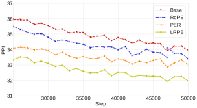
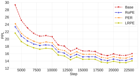
Figure 2: The validation result of Autoregressive language model on the Wikitext-103 dataset(left) and Roberta on the Wikibook dataset(right). In both cases, the best result of the proposed LRPE has a better PPL and faster convergence speed than competing methods.

Competing methods

Our baseline (marked as Base) is a Linear Transformer with $1+\mathrm{elu}(\cdot)$ (Katharopoulos et al., 2020) as the kernel function with sinusoidal positional encoding (Vaswani et al., 2017). For comparison, we also choose several state-of-the-art methods, i.e., RoPE (Su et al., 2021), SPE (Liutkus et al., 2021), PermuteFormer (abbreviated as “PER”) (Chen, 2021).

4.2 Results

Table 2: Quantitative results of the autoregressive language model on the WikiText-103 and Books dataset. The best result is highlighted with bold and the second best with underlined. $\downarrow$ means smaller is better.

Method	Wikitext-103		Books
	Val$\downarrow$	Test$\downarrow$	Val$\downarrow$	Test$\downarrow$
Base	33.94	33.74	9.12	8.78
Rope	33.40	33.13	8.98	8.65
SPE	43.50	41.91	11.91	10.85
PER	32.86	32.53	8.53	8.20
Type1	31.90	31.60	8.52	8.19
Type2	31.95	31.71	8.46	8.14
Type3	33.90	33.95	8.69	8.43

Autoregressive language model. The autoregressive language model has 6 decoder layers and is trained on the WikiText-103 dataset (Merity et al., 2017). In order to test the performance of the method on long sequence modeling, we tested the performance of the model on the Books (Zhu et al., 2015) dataset. We use the Perplexity (PPL) as the evaluation metric and report the results in Table 2. We observe that all variants of LRPE present a performance gain over the baseline. Notably, Type 1 and Type 2 models achieve the best performance on Wikitext-103 and Books, respectively, demonstrating superior capability in language modeling.

Table 3: Quantitative results of image classification on the ImageNet-1k dataset. The best result is highlighted with bold and the second with underlined. $\uparrow$ means larger is better

Method	Acc$\uparrow$	Params
Base	77.88	22.04
RoPE	78.52	22.04
PER	77.99	22.04
Type1	78.58	22.05
Type2	78.78	22.05
Type3	77.74	22.05

Bidirectional language model. The bidirectional model follows an encoder-only structure, i.e., Roberta (Liu et al., 2020), with 12 layers. In order to verify the performance of the model on a large data set, we adopt the Wikibook dataset used by Wettig et al. (2022) for pre-training and used their configurations to update 23k times. The results are in Table 1 and Figure 2. In the pre-training phase, LRPE outperforms all competitors. Next, we fine-tune the model for the GLUE task. As shown in Table 1, our method outperforms competing methods on all tasks with a clear margin.

Image classification model. To verify the robustness and effectiveness of LRPE  under different modal tasks, we test our method on the computer vision domain. Specifically, we conduct experiments on Imagenet-1k Deng et al. (2009) dataset using the Deit-small architecture Touvron et al. (2021) on the image classification task. In particular, we replace the Attention with Linear Attention Katharopoulos et al. (2020) and then adopt various relative positional encoding. As shown in Table 3, LRPE beats all the competing methods.

Long-Range Arena. In order to validate the effectiveness of LRPE on long-sequence modeling tasks, we conducted experiments on Long-Range Arena benchmark (Tay et al., 2020). As shown in Table 4, LRPE has positive effects on almost all tasks.

Table 4: Quantitative results of classification tasks on the Long-Range Arena benchmark. The best result is highlighted with bold and the second with underlined. $\uparrow$ means larger is better.

Model	Text	ListOps	Retrieval	Pathfinder	Image	AVG
Base	64.81	39.17	84.71	71.61	41.21	60.30
RoPE	66.53	40.57	78.75	72.68	62.50	64.59
Per	65.50	39.17	83.40	69.55	42.03	60.86
Type1	66.80	39.84	82.13	73.79	63.43	65.47
Type2	66.52	39.79	81.55	73.46	62.35	65.03
Type3	64.94	39.56	83.86	70.78	45.15	61.54

4.3 Discussion

An explanation of LRPE.

Table 5: Ablation results with different rotation matrix $\mathbf{P}$ for language modeling on the WikiText-103 dataset.

	Unitary	Orthogonal	Permutation	Avg.
Householder	31.90	31.95	33.90	32.58
Identity	32.04	31.86	34.53	32.80
Permutation	32.09	31.59	34.16	32.61

According to the discussion in Section. 3.3, The proposed LRPE rotates the token feature through $\mathbf{P}$, and encodes the positional information through $\mathbf{\Lambda}^{(s)}$ . In Table 5, we ablate the effectiveness of the $\mathbf{P}$ matrix on the autoregressive language modeling task. Our approach with the Householder matrix achieves better results than the one equipped with other metrics. It indicates that we can get better performance by carefully selecting the projection of the positional encoding.

Table 6: Training speed of different methods on the bidirectional language model. The value standards for the speed relative to the base method. $\uparrow$ means larger is faster.

Method	Relative speed$\uparrow$
Base	1.00
Rope	0.86
SPE	0.61
PER	0.94
Type1	0.82
Type2	0.82
Type3	0.89

Complexity and efficiency.

The implementation of the proposed LRPE does not affect the computational complexity of the linear transformer, i.e., preserving the linear complexity as $O(n)$. We also measure the training speed of the bidirectional language model on the same local machine and observe that the speed after using LRPE is only a bit slower than the baseline on average. The detailed comparison of the efficiency can be found in Table 6. In general, LRPE does not incur a significant computational burden to the transformer, and can fulfill the practical needs by maintaining comparable efficiency.

5 Conclusion

In this paper, we standardize the form of relative positional encoding for linear attention. The unitary transformation is employed as a special solution to the linearized relative positional encoding, and the solutions as per various constraints constitute the unitary relative positional encoding (LRPE) family. We validate the effectiveness of LRPE through extensive experiments on both natural language processing and computer vision tasks with different transformer architectures. It outperforms competing methods in all tasks. In addition, it highlights a broad paradigm for formulating linear transformer-applicable positional encoding techniques that are more generically relative.

Appendix A Mathematical Notations

Notation	Meaning
$\mathbf{X}$	Hidden state.
$\mathbf{Q},\mathbf{K},\mathbf{V}$	Query, key, value.
$\mathbf{W}_{Q},\mathbf{W}_{K},\mathbf{W}_{V}$	Weight matrices for $\mathbf{Q}$,$\mathbf{K}$,$\mathbf{V}$.
$\mathbf{O}$	Attention output.
$\mathbf{m}^{\mkern-1.5mu\mathsf{T}}_{s}$	$s$-th row of matrix $M$ (real domain).
$\mathbf{m}^{\mathsf{H}}_{s}$	$s$-th row of matrix $M$ (complex domain).
$\phi$	Kernel function for linear attention.
$\mathbf{1}_{d}$	All-ones vector with dimention $d$.
$\mathbf{I}_{d}$	Identity matrix with dimention $d$.
block-diag	Combining matrices into larger
	block diagonal matrices as in Eq. 25

Table 7: Mathematical notations used in the paper.

$$\text{block-diag}\{\mathbf{W}_{1},\mathbf{W}_{2},\ldots,\mathbf{W}_{n}\}=\left[\begin{matrix}\mathbf{W}_{1}&&\\ &\mathbf{W}_{2}&\\ &&\ddots\\ &&&\mathbf{W}_{n}\end{matrix}\right].$$ (25)

Appendix B Computation of Vanilla/Linear Attention

B.1 Basic Notations

Both vanilla and linear attention blocks involve three matrices, i.e., $\mathbf{Q}$ (Query), $\mathbf{K}$ (Key) and $\mathbf{V}$ (Value). All of them are linear projections of input $\mathbf{X}\in\mathbb{C}^{n\times d}$, i.e.,

$$\mathbf{X} =\left[\begin{matrix}\mathbf{x}_{1}^{\mkern-1.5mu\mathsf{T}}\\ \vdots\\ \mathbf{x}_{n}^{\mkern-1.5mu\mathsf{T}}\end{matrix}\right]\in\mathbb{R}^{n\times d},$$ (26)

$$\mathbf{Q} =\left[\begin{matrix}\mathbf{q}_{1}^{\mkern-1.5mu\mathsf{T}}\\ \vdots\\ \mathbf{q}_{n}^{\mkern-1.5mu\mathsf{T}}\end{matrix}\right]=\mathbf{XW}_{Q}=\left[\begin{matrix}\mathbf{x}_{1}^{\mkern-1.5mu\mathsf{T}}\mathbf{W}_{Q}\\ \vdots\\ \mathbf{x}_{n}^{\mkern-1.5mu\mathsf{T}}\mathbf{W}_{Q}\end{matrix}\right]\in\mathbb{R}^{n\times d},$$

$$\mathbf{K} =\left[\begin{matrix}\mathbf{k}_{1}^{\mkern-1.5mu\mathsf{T}}\\ \vdots\\ \mathbf{k}_{n}^{\mkern-1.5mu\mathsf{T}}\end{matrix}\right]=\mathbf{XW}_{K}=\left[\begin{matrix}\mathbf{x}_{1}^{\mkern-1.5mu\mathsf{T}}\mathbf{W}_{K}\\ \vdots\\ \mathbf{x}_{n}^{\mkern-1.5mu\mathsf{T}}\mathbf{W}_{K}\end{matrix}\right]\in\mathbb{R}^{n\times d},$$

$$\mathbf{V} =\left[\begin{matrix}\mathbf{v}_{1}^{\mkern-1.5mu\mathsf{T}}\\ \vdots\\ \mathbf{v}_{n}^{\mkern-1.5mu\mathsf{T}}\end{matrix}\right]=\mathbf{XW}_{V}=\left[\begin{matrix}\mathbf{x}_{1}^{\mkern-1.5mu\mathsf{T}}\mathbf{W}_{V}\\ \vdots\\ \mathbf{x}_{n}^{\mkern-1.5mu\mathsf{T}}\mathbf{W}_{V}\end{matrix}\right]\in\mathbb{R}^{n\times d},$$

where $\mathbf{W}_{Q},\mathbf{W}_{K},\mathbf{W}_{V}\in\mathbb{R}^{d\times d}$.

The vector form is organized as

$$\begin{gathered}\mathbf{q}_{s}=\mathbf{W}_{Q}^{\mkern-1.5mu\mathsf{T}}\mathbf{x}_{s},\mathbf{k}_{s}=\mathbf{W}_{K}^{\mkern-1.5mu\mathsf{T}}\mathbf{x}_{s},\mathbf{v}_{s}=\mathbf{W}_{V}^{\mkern-1.5mu\mathsf{T}}\mathbf{x}_{s}.\end{gathered}$$ (27)

The attention output is

$$\mathbf{O}=\left[\begin{matrix}\mathbf{o}_{1}^{\mkern-1.5mu\mathsf{T}}\\ \vdots\\ \mathbf{o}_{n}^{\mkern-1.5mu\mathsf{T}}\end{matrix}\right]\in\mathbb{R}^{n\times d}.$$ (28)

B.2 Vanilla Attention

In vanilla attention, the output is computed using the Softmax weighted sum, i.e.,

$$\mathbf{o}_{s} =\textrm{Attention}(\mathbf{q}_{s},\mathbf{K},\mathbf{V})$$ (29)

$$=\sum_{t=1}^{n}\mathbf{a}_{st}\mathbf{v}_{t}$$

$$=\sum_{t=1}^{n}\frac{\exp\left(\mathbf{q}_{s}^{\mkern-1.5mu\mathsf{T}}\mathbf{k}_{t}/\sqrt{d}\right)\mathbf{v}_{t}}{\sum_{r=1}^{n}\exp\left(\mathbf{q}_{s}^{\mkern-1.5mu\mathsf{T}}\mathbf{k}_{r}/\sqrt{d}\right)},$$

$$\mathbf{O} =\textrm{Softmax}(\mathbf{QK}^{\mkern-1.5mu\mathsf{T}}/\sqrt{d})\mathbf{V}.$$

B.3 Linear Attention

The linear attention is formulated as follows,

$$\mathbf{o}_{s} =\textrm{LinearAttention}(\mathbf{q}_{s},\mathbf{K},\mathbf{V})$$ (30)

$$=\sum_{t=1}^{n}\mathbf{a}_{st}\mathbf{v}_{t}$$

$$=\sum_{t=1}^{n}\frac{\phi(\mathbf{q}_{s})^{\mkern-1.5mu\mathsf{T}}\phi(\mathbf{k}_{t})}{\sum_{t=1}^{n}\phi(\mathbf{q}_{s})^{\mkern-1.5mu\mathsf{T}}\phi(\mathbf{k}_{t})}\mathbf{v}_{t}$$

$$=\frac{\sum_{t=1}^{n}\phi(\mathbf{q}_{s})^{\mkern-1.5mu\mathsf{T}}\phi(\mathbf{k}_{t})\mathbf{v}_{t}}{\sum_{t=1}^{n}\phi(\mathbf{q}_{s})^{\mkern-1.5mu\mathsf{T}}\phi(\mathbf{k}_{t})}$$

$$=\phi(\mathbf{q}_{s})^{\mkern-1.5mu\mathsf{T}}\frac{\sum_{t=1}^{n}\phi(\mathbf{k}_{t})\mathbf{v}_{t}}{\phi(\mathbf{q}_{s})^{\mkern-1.5mu\mathsf{T}}\sum_{t=1}^{n}\phi(\mathbf{k}_{t})},$$

$$\mathbf{O} =\mathbf{\Delta}^{-1}\phi(\mathbf{Q})\phi(\mathbf{K})^{\mkern-1.5mu\mathsf{T}}\mathbf{V}$$

$$=\mathbf{\Delta}^{-1}\phi(\mathbf{Q})[\phi(\mathbf{K})^{\mkern-1.5mu\mathsf{T}}\mathbf{V}],$$

$$\mathbf{\Delta} =\mathrm{diag}(\phi(\mathbf{Q})[\phi(\mathbf{K})^{\mkern-1.5mu\mathsf{T}}{\mathbf{1}}_{n}]).$$

Appendix C Proof of Theorem

C.1 More Examples

In the following, we provide two additional examples of relative positional encoding with the canonical form.

DeBERTa (Huang et al., 2020):

$$f_{\mathrm{rel}}(\mathbf{q}_{s},\mathbf{k}_{t}) =\mathbf{q}_{s}^{\mathsf{H}}\mathbf{k}_{t}+\mathbf{q}_{s}^{\mathsf{H}}\mathbf{\bar{k}}_{{g(s-t)}}+\mathbf{\bar{q}}_{{g(t-s)}}^{\mathsf{H}}\mathbf{k}_{t},$$ (31)

$$g(x) =\begin{cases}0&x\leq-c\\ 2c-1&x\geq c\\ x+c&\text{others}.\end{cases}$$

The canonical form is

$$\begin{gathered}m=3,\\ \mathbf{\hat{q}}_{s}^{(1)}=\mathbf{q}_{s},\mathbf{\hat{k}}_{t}^{(1)}=\mathbf{k}_{t},\mathbf{W}_{t-s}^{(1)}=\mathbf{I}_{d},\\ \mathbf{\hat{q}}_{s}^{(2)}=\mathbf{q}_{s},\mathbf{\hat{k}}_{t}^{(2)}=\mathbf{I}_{d},\mathbf{W}_{t-s}^{(2)}=\frac{1}{d}\underbrace{\left[\begin{matrix}\mathbf{\bar{k}}_{{g(s-t)}}&\ldots&\mathbf{\bar{k}}_{{g(s-t)}}\end{matrix}\right]}_{d\text{ columns}},\\ \mathbf{\hat{q}}_{s}^{(3)}=\mathbf{I}_{d},\mathbf{\hat{k}}_{t}^{(3)}=\mathbf{k}_{t},\mathbf{W}_{t-s}^{(3)}=\frac{1}{d}\underbrace{\left[\begin{matrix}\mathbf{\bar{q}}_{{g(t-s)}}&\ldots&\mathbf{\bar{q}}_{{g(t-s)}}\end{matrix}\right]}_{d\text{ columns}}.\end{gathered}$$ (32)

RPR (Shaw et al., 2018):

$$f_{\mathrm{rel}}(\mathbf{q}_{s},\mathbf{k}_{t}) =\mathbf{q}_{s}^{\mathsf{H}}\mathbf{k}_{t}+\mathbf{q}_{s}^{\mathsf{H}}\mathbf{c}_{t-s},$$ (33)

$$\mathbf{c}_{t-s} =\mathbf{w}_{\mathrm{clip}(t-s,k)},$$

$$\mathrm{clip}(x,k) =\max(-k,\min(k,x)),$$

$$\mathbf{w_{s}} \in\mathbb{C}^{d},-k\leq s\leq k.$$

The canonical form is

$$\begin{gathered}m=2,\\ \mathbf{\hat{q}}_{s}^{(1)}=\mathbf{q}_{s},\mathbf{\hat{k}}_{t}^{(1)}=\mathbf{k}_{t},\mathbf{W}_{t-s}^{(1)}=\mathbf{I}_{d},\\ \mathbf{\hat{q}}_{s}^{(2)}=\mathbf{q}_{s},\mathbf{\hat{k}}_{t}^{(2)}=\mathbf{I}_{d},\mathbf{W}_{t-s}^{(2)}=\frac{1}{d}\underbrace{\left[\begin{matrix}\mathbf{c}_{t-s}&\ldots&\mathbf{c}_{t-s}\end{matrix}\right]}_{d\text{ columns}}.\end{gathered}$$ (34)

cosFormer (Qin et al., 2022b):

$$f_{\mathrm{rel}}(\mathbf{q}_{s},\mathbf{k}_{t})=\mathbf{q}_{s}^{\mathsf{H}}\mathbf{k}_{t}\cos(\alpha(t-s)),$$ (35)

which indicates that the relative positional encoding is effectively a coefficient term in the attention matrix, as such, it can be derived via a positional matrix primitive with the coefficients.

$$\begin{gathered}m=1,\\ \mathbf{\hat{q}}_{s}^{(1)}=\mathbf{q}_{s},\mathbf{\hat{k}}_{t}^{(1)}=\mathbf{k}_{t},\mathbf{W}_{t-s}^{(1)}=\cos(\alpha(t-s))\mathbf{I}_{d}.\end{gathered}$$ (36)

C.2 Speed analysis

Proof of Lrpe speed.

For this, we only need to prove that the time complexity is linear with respect to $n$. To this end, we first give basic notations as follows,

$$\mathbf{Q}=\left[\begin{matrix}\mathbf{q}_{1}^{\mathsf{H}}\\ \vdots\\ \mathbf{q}_{n}^{\mathsf{H}}\end{matrix}\right]\in\mathbb{C}^{n\times d},\mathbf{K}=\left[\begin{matrix}\mathbf{k}_{1}^{\mathsf{H}}\\ \vdots\\ \mathbf{k}_{n}^{\mathsf{H}}\end{matrix}\right]\in\mathbb{C}^{n\times d},\mathbf{V}=\left[\begin{matrix}\mathbf{v}_{1}^{\mathsf{H}}\\ \vdots\\ \mathbf{v}_{n}^{\mathsf{H}}\end{matrix}\right]\in\mathbb{C}^{n\times d},$$ (37)

$$\tilde{\mathbf{Q}}=\left[\begin{matrix}(\mathbf{M}_{1}\mathbf{q}_{1})^{\mathsf{H}}\\ \vdots\\ (\mathbf{M}_{n}\mathbf{q}_{n})^{\mathsf{H}}\end{matrix}\right]\in\mathbb{C}^{n\times d},\tilde{\mathbf{K}}=\left[\begin{matrix}(\mathbf{M}_{1}\mathbf{k}_{1})^{\mathsf{H}}\\ \vdots\\ (\mathbf{M}_{n}\mathbf{k}_{n})^{\mathsf{H}}\end{matrix}\right]\in\mathbb{C}^{n\times d}.$$

The time complexity of transforming $\mathbf{Q},\mathbf{K}$ to $\tilde{\mathbf{Q}},\tilde{\mathbf{K}}$ is $O(nd^{2})$. The next step is to calculate the output, i.e.,

$$\mathbf{O} =\mathbf{Q}(\mathbf{K}^{\mathsf{H}}\mathbf{V})\in\mathbb{C}^{n\times d},$$ (38)

$$\mathbf{O} =\mathbf{\Delta}^{-1}\tilde{\mathbf{Q}}\tilde{\mathbf{K}}^{\mathsf{H}}\mathbf{V}$$

$$=\mathbf{\Delta}^{-1}\tilde{\mathbf{Q}}[\tilde{\mathbf{K}}^{\mathsf{H}}\mathbf{V}],$$

$$\mathbf{\Delta} =\mathrm{diag}(\tilde{\mathbf{Q}})[\tilde{\mathbf{K}}^{\mathsf{H}}{\mathbf{1}}_{n}].$$

Clearly, Eq. 38 is a standard formulation for the linear attention with the time complexity as $O(nd^{2})$. Combing it with the first step, we have the total time complexity as $O(nd^{2})$, which is unchanged. ∎

C.3 Linearized Relative Positional Encoding

Before the proof, we first give the following theorems (Yao & Algebra, 2015):

Theorem C.1.

If matrix $\mathbf{W}\in\mathbb{C}^{d\times d}$ is a unitary matrix, there exists another unitary matrix $\mathbf{P}\in\mathbb{C}^{d\times d}$, such that

$$\mathbf{W} =\mathbf{P}^{\mathsf{H}}\Lambda\mathbf{P},$$ (39)

$$\mathbf{\Lambda} =\mathrm{diag}\{\exp(i\theta_{1}),\ldots,\exp(i\theta_{d})\},$$

$$i^{2} =-1.$$

Theorem C.2.

If matrix $\mathbf{W}\in\mathbb{R}^{d\times d}$ is an orthogonal matrix, there exists another orthogonal matrix $\mathbf{P}\in\mathbb{R}^{d\times d}$, such that

$$\mathbf{W} =\mathbf{P}^{\mkern-1.5mu\mathsf{T}}\mathbf{\Lambda}\mathbf{P},$$ (40)

$$\mathbf{\Lambda} =\mathrm{diag}\{\mathbf{\Lambda}_{1},\ldots,\mathbf{\Lambda}_{r};1,\ldots,1;-1,\ldots,-1\},$$

$$\mathbf{\Lambda}_{k} =\left[\begin{matrix}\cos\theta_{k}&-\sin\theta_{k}\\ \sin\theta_{k}&\cos\theta_{k}\end{matrix}\right],k=1,\ldots r.$$

C.4 Unitary (Solution 1)

Proof of Proposition 3.3.

According to Theorem C.1, we can assume that $\mathbf{W}_{s}$ has the following form ($\mathbf{P}\in\mathbb{C}^{d\times d}$ is a unitary matrix),

$$\mathbf{W}_{s} =\mathbf{P}^{\mathsf{H}}\mathbf{\Lambda}^{(s)}\mathbf{P},$$ (41)

$$\mathbf{\Lambda}^{(s)} =\mathrm{diag}\{\exp(i\theta_{1}^{(s)}),\ldots,\exp(i\theta_{d}^{(s)})\}.$$

Hence, Eq. 14 is equivalent to

$$\mathbf{W}_{s}^{\mathsf{H}}\mathbf{W}_{t} =\mathbf{W}_{t-s},$$ (42)

$$\mathbf{P}^{\mathsf{H}}{\Lambda^{(s)}}^{\mathsf{H}}\mathbf{P}\mathbf{P}^{\mathsf{H}}\Lambda^{(t)}\mathbf{P} =\mathbf{P}^{\mathsf{H}}\Lambda^{(t-s)}\mathbf{P},$$

$$\mathbf{P}^{\mathsf{H}}{\mathbf{\Lambda}^{(s)}}^{\mathsf{H}}\mathbf{\Lambda}^{(t)}\mathbf{P} =\mathbf{P}^{\mathsf{H}}\mathbf{\Lambda}^{(t-s)}\mathbf{P},$$

$${\mathbf{\Lambda}^{(s)}}^{\mathsf{H}}\mathbf{\Lambda}^{(t)} =\mathbf{\Lambda}^{(t-s)},$$

$$\mathrm{diag}\left\{j(\theta_{1}^{(t)}-\theta_{1}^{(s)}),j(\theta_{2}^{(t)}-\theta_{2}^{(s)}),\cdots,j(\theta_{d}^{(t)}-\theta_{d}^{(s)})\right\} =\mathrm{diag}\left\{j\theta_{1}^{(t-s)},j\theta_{2}^{(t-s)},\cdots,j\theta_{d}^{(t-s)}\right\}.$$

In this case, $\forall k=1,\ldots,d$, we have

$$\theta_{k}^{(t)}-\theta_{k}^{(s)}=\theta_{k}^{(t-s)}+2l\pi,k,l\in\mathbb{Z}.$$ (43)

Note that $2l\pi$ does not affect the result, so we can assume $l=0$, i.e.,

$$\theta_{k}^{(t)}-\theta_{k}^{(s)}=\theta_{k}^{(t-s)}.$$ (44)

Taking $t=s+1$, we get

$$\theta_{k}^{(s+1)}-\theta_{k}^{(s)}=\theta_{k}^{(1)},$$ (45)

$$\theta_{k}^{(s)}=s\theta^{(1)}_{k}\triangleq s\alpha_{k}.$$

∎

C.5 Orthogonal (Solution 2)

Proof of Proposition 3.4.

According to Theorem C.2, we can assume that $\mathbf{W}_{s}$ has the following form ($\mathbf{P}\in\mathbb{R}^{d\times d}$ is an orthogonal matrix),

$$\mathbf{W}_{s} =\mathbf{P}^{\mkern-1.5mu\mathsf{T}}\mathbf{\Lambda}^{(s)}\mathbf{P},$$ (46)

$$\mathbf{\Lambda}^{(s)} =\left[\begin{matrix}\mathbf{A}^{(s)}&&\\ &\mathbf{B}^{(s)}&\\ &&\mathbf{C}^{(s)}\end{matrix}\right],$$

$$\mathbf{A}^{(s)} =\left[\begin{matrix}\mathbf{A}_{1}^{(s)}&\\ &\ddots\\ &&\mathbf{A}_{n}^{(s)}\\ \end{matrix}\right]\in\mathbb{R}^{2p\times 2p},$$

$$\mathbf{B}^{(s)} =\mathbf{I}_{q}\in\mathbb{R}^{q\times q},$$

$$\mathbf{C}^{(s)} =\mathbf{-}\mathbf{I}_{r}\in\mathbb{R}^{r\times r},$$

$$\mathbf{A}_{k}^{(s)} =\left[\begin{matrix}\cos\theta_{k}^{(s)}&-\sin\theta_{k}^{(s)}\\ \sin\theta_{k}^{(s)}&\cos\theta_{k}^{(s)}\end{matrix}\right].$$

Hence, Eq. 14 is equivalent to

$$\mathbf{W}_{s}^{\mkern-1.5mu\mathsf{T}}\mathbf{W}_{t} =\mathbf{W}_{t-s},$$ (47)

$$\mathbf{P}^{\mkern-1.5mu\mathsf{T}}{\mathbf{\Lambda}^{(s)}}^{\mkern-1.5mu\mathsf{T}}\mathbf{P}\mathbf{P}^{\mkern-1.5mu\mathsf{T}}\mathbf{\Lambda}^{(t)}\mathbf{P} =\mathbf{P}^{\mkern-1.5mu\mathsf{T}}\mathbf{\Lambda}^{(t-s)}\mathbf{P},$$

$$\mathbf{P}^{\mkern-1.5mu\mathsf{T}}{\mathbf{\Lambda}^{(s)}}^{\mkern-1.5mu\mathsf{T}}\mathbf{\Lambda}^{(t)}\mathbf{P} =\mathbf{P}^{\mkern-1.5mu\mathsf{T}}\mathbf{\Lambda}^{(t-s)}\mathbf{P},$$

$${{\mathbf{\Lambda}}^{(s)}}^{\mkern-1.5mu\mathsf{T}}\mathbf{\Lambda}^{(t)} =\mathbf{\Lambda}^{(t-s)},$$

$$\left[\begin{matrix}{\mathbf{A}^{(s)}}^{\mkern-1.5mu\mathsf{T}}&&\\ &{\mathbf{B}^{(s)}}^{\mkern-1.5mu\mathsf{T}}&\\ &&{\mathbf{C}^{(s)}}^{\mkern-1.5mu\mathsf{T}}\end{matrix}\right]\left[\begin{matrix}\mathbf{A}^{(t)}&&\\ &\mathbf{B}^{(t)}&\\ &&\mathbf{C}^{(t)}\end{matrix}\right] =\left[\begin{matrix}\mathbf{A}^{(t-s)}&&\\ &\mathbf{B}^{(t-s)}&\\ &&\mathbf{C}^{(t-s)}\end{matrix}\right],$$

where

$${\mathbf{A}^{(s)}}^{\mkern-1.5mu\mathsf{T}}\mathbf{A}^{(t)} =\mathbf{A}^{(t-s)},$$ (48)

$${\mathbf{B}^{(s)}}^{\mkern-1.5mu\mathsf{T}}\mathbf{B}^{(t)} =\mathbf{B}^{(t-s)},$$

$${\mathbf{C}^{(s)}}^{\mkern-1.5mu\mathsf{T}}\mathbf{C}^{(t)} =\mathbf{C}^{(t-s)}.$$

For $\mathbf{A}^{(s)}$, considering the $k$-th component, we get

$${\mathbf{A}^{(s)}_{k}}^{\mkern-1.5mu\mathsf{T}}{\mathbf{A}}^{(t)}_{k} ={\mathbf{A}}^{(t-s)}_{k}$$ (49)

$$=\left[\begin{array}[]{cc}\cos\theta^{(s)}_{k}&\sin\theta^{(s)}_{k}\\ -\sin\theta^{(s)}_{k}&\cos\theta^{(s)}_{k}\end{array}\right]\left[\begin{array}[]{cc}\cos\theta^{(t)}_{k}&-\sin\theta^{(t)}_{k}\\ \sin\theta^{(t)}_{k}&\cos\theta^{(t)}_{k}\end{array}\right]$$

$$=\left[\begin{array}[]{cc}\cos\theta^{(s)}_{k}\cos\theta^{(t)}_{k}+\sin\theta^{(s)}_{k}\cos\theta^{(t)}_{k}&\sin\theta^{(s)}_{k}\cos\theta^{(t)}_{k}-\cos\theta^{(s)}_{k}\sin\theta^{(t)}_{k}\\ -\sin\theta^{(s)}_{k}\cos\theta^{(t)}_{k}+\cos\theta^{(s)}_{k}\sin\theta^{(t)}_{k}&\cos\theta^{(s)}_{k}\cos\theta^{(t)}_{k}+\sin\theta^{(s)}_{k}\sin\theta^{(t)}_{k}\end{array}\right]$$

$$=\left[\begin{array}[]{cc}\cos\left(\theta^{(t)}_{k}-\theta^{(s)}_{k}\right)&-\sin\left(\theta^{(t)}_{k}-\theta^{(s)}_{k}\right)\\ \sin\left(\theta^{(t)}_{k}-\theta^{(s)}_{k}\right)&\cos\left(\theta^{(t)}_{k}-\theta^{(s)}_{k}\right)\\ \end{array}\right]$$

$$=\mathbf{A}^{(t-s)}_{k}$$

$$=\left[\begin{array}[]{cc}\cos\theta^{(t-s)}_{k}&-\sin\theta^{(t-s)}_{k}\\ \sin\theta^{(t-s)}_{k}&\cos\theta^{(t-s)}_{k}\end{array}\right].$$

Hence, $\forall k=1,\ldots,d$, we have

$$\theta_{k}^{(t)}-\theta_{k}^{(s)}=\theta_{k}^{(t-s)}+2k\pi,k\in\mathbb{Z}.$$ (50)

Note that $2t\pi$ does not affect the result, so we can assume $t=0$, i.e.,

$$\theta_{k}^{(t)}-\theta_{k}^{(s)}=\theta_{k}^{(t-s)}.$$ (51)

Taking $t=s+1$, we have

$$\theta_{k}^{(s+1)}-\theta_{k}^{(s)}=\theta_{k}^{(1)},$$ (52)

$$\theta_{k}^{(s)}=s\theta^{(1)}_{k}\triangleq s\alpha_{k}.$$

Next, for $\mathbf{B}^{(s)}$, the conclusion is more obvious, i.e.,

$${\mathbf{B}^{(s)}}^{\mkern-1.5mu\mathsf{T}}\mathbf{B}^{(t)} =\mathbf{I}_{q}^{\mkern-1.5mu\mathsf{T}}\mathbf{I}_{q}$$ (53)

$$=\mathbf{I}_{q}$$

$$=\mathbf{B}^{(t-s)}.$$

Finally, for $\mathbf{C}^{(s)}$, we have

$${\mathbf{C}^{(s)}}^{\mkern-1.5mu\mathsf{T}}\mathbf{C}^{(t)} =(-\mathbf{I}_{r}^{T})(-\mathbf{I}_{r})$$ (54)

$$=\mathbf{I}_{r}$$

$$\neq\mathbf{C}^{(t-s)}.$$

In that case, we must have $r=0$.

∎

C.6 Permutation

Prior to the proof, we first provide some relevant definitions and propositions.

Definition C.3.

Permutation $\pi$ is a bijection defined on the integer set:

$$\pi:\{1,2,\cdots,d\}\rightarrow\{1,2,\cdots,d\},d\in\mathbb{Z}^{+}.$$ (55)

Definition C.4.

For matrix

$$\mathbf{M}=\left[\begin{matrix}\mathbf{m}_{1}^{\mkern-1.5mu\mathsf{T}}\\ \mathbf{m}_{2}^{\mkern-1.5mu\mathsf{T}}\\ \vdots\\ \mathbf{m}_{d}^{\mkern-1.5mu\mathsf{T}}\end{matrix}\right]\in\mathbb{R}^{d\times d},\mathbf{m}_{k}\in\mathbb{R}^{d},k=1,\ldots,d,$$ (56)

$\mathbf{M}_{\pi}$ is defined as

$$\mathbf{M}_{\pi}=\left[\begin{matrix}\mathbf{m}_{\pi(1)}^{\mkern-1.5mu\mathsf{T}}\\ \mathbf{m}_{\pi(2)}^{\mkern-1.5mu\mathsf{T}}\\ \vdots\\ \mathbf{m}_{\pi(d)}^{\mkern-1.5mu\mathsf{T}}\end{matrix}\right].$$ (57)

Definition C.5.

For identity matrix $\mathbf{I}_{d}\in\mathbb{R}^{d\times d}$ and permutation $\pi$, we define

$$\mathbf{\Lambda}_{k}=(\mathbf{I}_{d})_{\pi^{k}}.$$ (58)

For $\mathbf{\Lambda}_{k}$, we have the following important properties:

Lemma C.6.

For permutation $\pi$, matrix $\mathbf{M}\in\mathbb{R}^{d\times d}$ and $\mathbf{\Lambda}_{k}\in\mathbb{R}^{d\times d}$ defined in C.5, we have

$$\mathbf{M}_{\pi}=\mathbf{\Lambda}_{1}\mathbf{M}.$$ (59)

Proof.

We first organize $\mathbf{I}_{d}\in\mathbb{R}^{d\times d}$ in the following form, where $\mathbf{e}_{k}\in\mathbb{R}^{d},k=1,\ldots,d$ represents the one-hot vector with the $k$-th element as one, i.e.,

$$\mathbf{I}_{d}=\left[\begin{array}[]{c}{\mathbf{e}}_{1}^{\mkern-1.5mu\mathsf{T}}\\ {\mathbf{e}}_{2}^{\mkern-1.5mu\mathsf{T}}\\ \vdots\\ {\mathbf{e}}_{d}^{\mkern-1.5mu\mathsf{T}}\end{array}\right].$$ (60)

Notice that

$$\mathbf{e}_{k}^{\mkern-1.5mu\mathsf{T}}\mathbf{M}=\mathbf{m}_{k}^{\mkern-1.5mu\mathsf{T}},$$ (61)

so we get

$$\mathbf{\Lambda}_{1}\mathbf{M} =\left[\begin{array}[]{c}{\mathbf{e}}_{\pi(1)}^{\mkern-1.5mu\mathsf{T}}\\ {\mathbf{e}}_{\pi(2)}^{\mkern-1.5mu\mathsf{T}}\\ \vdots\\ {\mathbf{e}}_{\pi(d)}^{\mkern-1.5mu\mathsf{T}}\end{array}\right]\mathbf{M}$$ (62)

$$=\left[\begin{array}[]{c}{\mathbf{e}}_{\pi(1)}^{\mkern-1.5mu\mathsf{T}}\mathbf{M}\\ {\mathbf{e}}_{\pi(2)}^{\mkern-1.5mu\mathsf{T}}\mathbf{M}\\ \vdots\\ {\mathbf{e}}_{\pi(d)}^{\mkern-1.5mu\mathsf{T}}\mathbf{M}\end{array}\right]$$

$$=\left[\begin{array}[]{c}\mathbf{m}_{\pi(1)}^{\mkern-1.5mu\mathsf{T}}\\ \mathbf{m}_{\pi(2)}^{\mkern-1.5mu\mathsf{T}}\\ \vdots\\ \mathbf{m}_{\pi(d)}^{\mkern-1.5mu\mathsf{T}}\end{array}\right]$$

$$=\mathbf{M}_{\pi}.$$

∎

Theorem C.7.

For $\mathbf{\Lambda}_{k}$ defined in C.5, we have:

$$\mathbf{\Lambda}_{k}=\mathbf{\Lambda}_{1}^{k}.$$ (63)

Proof.

We use induction for the proof.

For $k=1$, the conclusion is obvious. Now assuming that the conclusion holds for $k=s-1$, when $k=s$, we have

$$\mathbf{\Lambda}_{s} =(\mathbf{I}_{d})_{\pi^{s}}$$ (64)

$$=((\mathbf{I}_{d})_{\pi^{s-1}})_{\pi}$$

$$=(\mathbf{\Lambda}_{s-1})_{\pi}$$

$$=(\mathbf{\Lambda}_{1}^{s-1})_{\pi}.$$

The next step is to prove

$$(\mathbf{\Lambda}_{1}^{s-1})_{\pi}=\mathbf{\Lambda}_{1}^{s}=\mathbf{\Lambda}_{1}\mathbf{\Lambda}_{1}^{s-1}.$$ (65)

The above conclusion follows from C.6.

∎

Theorem C.8.

$\mathbf{\Lambda}_{k}\in\mathbb{R}^{d\times d}$ defined in C.5 are orthogonal matrices, i.e.,

$$\mathbf{\Lambda}_{k}\mathbf{\Lambda}_{k}^{T}=\mathbf{\Lambda}_{k}^{\mkern-1.5mu\mathsf{T}}\mathbf{\Lambda}_{k}=\mathbf{I}_{d}.$$ (66)

Proof.

We first prove that the conclusion holds for $k=1$:

$$\mathbf{\Lambda}_{1}\mathbf{\Lambda}_{1}^{\mkern-1.5mu\mathsf{T}} =\left[\begin{array}[]{c}{\mathbf{e}}_{\pi(1)}^{\mkern-1.5mu\mathsf{T}}\\ {\mathbf{e}}_{\pi(2)}^{\mkern-1.5mu\mathsf{T}}\\ \vdots\\ {\mathbf{e}}_{\pi(d)}^{\mkern-1.5mu\mathsf{T}}\end{array}\right]\left[\begin{matrix}{\mathbf{e}}_{\pi(1)}&{\mathbf{e}}_{\pi(2)}&\ldots&{\mathbf{e}}_{\pi(d)}\end{matrix}\right],$$ (67)

$$\left[\mathbf{\Lambda}_{1}\mathbf{\Lambda}_{1}^{\mkern-1.5mu\mathsf{T}}\right]_{st} ={\mathbf{e}}_{\pi(s)}^{\mkern-1.5mu\mathsf{T}}{\mathbf{e}}_{\pi(t)}$$

$$=\delta_{st},$$

$$\mathbf{\Lambda}_{1}\mathbf{\Lambda}_{1}^{\mkern-1.5mu\mathsf{T}} =\mathbf{I}_{d}.$$

Since $\mathbf{\Lambda}_{1}$ is a square matrix, we also have

$$\mathbf{\Lambda}_{1}^{\mkern-1.5mu\mathsf{T}}\mathbf{\Lambda}_{1}=\mathbf{I}_{d}.$$ (68)

In general cases, we only use C.7, i.e.,

$$\mathbf{\Lambda}_{k}\mathbf{\Lambda}_{k}^{\mkern-1.5mu\mathsf{T}} =\mathbf{\Lambda}_{1}^{k}(\mathbf{\Lambda}_{1}^{k})^{\mkern-1.5mu\mathsf{T}}$$ (69)

$$=\mathbf{\Lambda}_{1}^{k}(\mathbf{\Lambda}_{1}^{\mkern-1.5mu\mathsf{T}})^{k}$$

$$=\mathbf{\Lambda}_{1}^{k-1}\mathbf{\Lambda}_{1}\mathbf{\Lambda}_{1}^{\mkern-1.5mu\mathsf{T}}(\mathbf{\Lambda}_{1}^{\mkern-1.5mu\mathsf{T}})^{k-1}$$

$$=\mathbf{\Lambda}_{1}^{k-1}(\mathbf{\Lambda}_{1}^{\mkern-1.5mu\mathsf{T}})^{k-1}$$

$$=\ldots$$

$$=\mathbf{I}_{d}.$$

With the same proof, we get

$$\mathbf{\Lambda}_{k}^{\mkern-1.5mu\mathsf{T}}\mathbf{\Lambda}_{k}=\mathbf{I}_{d}.$$ (70)

∎

Based on the above conclusions, we can prove Proposition 3.5 below.

Proof of Proposition 3.5.

According to Theorem C.8 and the product of the orthogonal matrix is an orthogonal matrix, we can assume that $\mathbf{W}_{k}$ has the following form ($\mathbf{P}\in\mathbb{R}^{d\times d}$ is an orthogonal matrix), i.e.,

$$\mathbf{W}_{k} =\mathbf{P}^{\mkern-1.5mu\mathsf{T}}\mathbf{\Lambda}^{(k)}\mathbf{P}.$$ (71)

The next step is to verify that it satisfies Eq. 14, which follows Theorem C.7 and C.8:

$$\mathbf{W}_{s}^{\mkern-1.5mu\mathsf{T}}\mathbf{W}_{t} =\mathbf{P}^{\mkern-1.5mu\mathsf{T}}{\mathbf{\Lambda}^{(s)}}^{\mkern-1.5mu\mathsf{T}}\mathbf{P}\mathbf{P}^{\mkern-1.5mu\mathsf{T}}{\mathbf{\Lambda}^{(t)}}\mathbf{P}$$ (72)

$$=\mathbf{P}^{\mkern-1.5mu\mathsf{T}}{\mathbf{\Lambda}^{(s)}}^{\mkern-1.5mu\mathsf{T}}{\mathbf{\Lambda}^{(t)}}\mathbf{P}$$

$$=\mathbf{P}^{\mkern-1.5mu\mathsf{T}}{\mathbf{\Lambda}^{(s)}}^{\mkern-1.5mu\mathsf{T}}(\mathbf{\Lambda}^{(1)})^{t}\mathbf{P}$$

$$=\mathbf{P}^{\mkern-1.5mu\mathsf{T}}{\mathbf{\Lambda}^{(s)}}^{\mkern-1.5mu\mathsf{T}}(\mathbf{\Lambda}^{(1)})^{s}(\mathbf{\Lambda}^{(1)})^{t-s}\mathbf{P}$$

$$=\mathbf{P}^{\mkern-1.5mu\mathsf{T}}{\mathbf{\Lambda}^{(s)}}^{\mkern-1.5mu\mathsf{T}}{\mathbf{\Lambda}^{(s)}}(\mathbf{\Lambda}^{(1)})^{t-s}\mathbf{P}$$

$$=\mathbf{P}^{\mkern-1.5mu\mathsf{T}}{\mathbf{\Lambda}^{(t-s)}}\mathbf{P}$$

$$=\mathbf{W}_{t-s}.$$

∎

Appendix D Implementation

D.1 Theory

LRPE($\mathbf{W}_{s}=\mathbf{P}^{\mathsf{H}}\mathbf{\Lambda}^{(s)}\mathbf{P}$) contains two components, i.e., the fixed unitary matrix $\mathbf{P}$ and the unitary matrix family $\mathbf{\Lambda}^{(s)}$ mentioned in proposition 3.3, 3.4, and 3.5. We first introduce the choice of matrices $\mathbf{P}/{\mathbf{\Lambda}}^{(s)}$, and then illustrate some implementation tricks.

Choice of matrices

For matrix $\mathbf{P}$, We list the species mentioned in the paper below:

• Householder matrix: denoted as a vector $\mathbf{v}\in\mathbb{R}^{d}$, i.e.,

  $$\mathbf{W}=\mathbf{I}_{d}-2\mathbf{v}\mathbf{v}^{\mkern-1.5mu\mathsf{T}}/(\mathbf{v}^{\mkern-1.5mu\mathsf{T}}\mathbf{v}).$$ (73)

  In our implementation, we sample $\mathbf{v}$ from a standard normal distribution, and make it deterministic.

• Permutation matrix: formulated as per the following permutation (inspired by Flash (Hua et al., 2022)), i.e.,

  $$\pi(2k)=k,\pi(2k+1)=\lfloor d/2\rfloor+1,1\leq 2k,2k+1\leq d.$$ (74)

• Identity matrix.

For matrix family $\mathbf{\Lambda}^{(s)}$, we use the following settings:

• For unitary (Solution 1) (3.3), we use the same method in (Su et al., 2021) with initialized $\alpha_{t}=10000^{-2t/d}$, and make it learnable.

• For orthogonal (Solution 2) (3.4), we choose the dimension of identity submatrix $q=0$ with initialized $\alpha_{t}=10000^{-2t/d}$ as in (Su et al., 2021) and make it learnable.

  • Another notable version to choose the dimension of the identity submatrix $q=0$ with initialized $\alpha_{t}=10000^{-2t/d}$ as in (Su et al., 2021), and make it deterministic. When using this version along with the identity matrix, we can get RoPE (Su et al., 2021).

• For permutation (Solution 3) (3.5), we randomly choose the permutation and make it deterministic.

  • Notice that when combing this method with identity matrix, we can get a version of PermuteFormer (Chen, 2021).

Implementation tricks

According to the following facts, we can simplify the computation, i.e.,

$$\mathbf{q}_{s}^{\mathsf{H}}\mathbf{W}_{s}^{\mathsf{H}}\mathbf{W}_{t}\mathbf{k}_{t} =\mathbf{q}_{s}^{\mathsf{H}}\mathbf{P}^{\mathsf{H}}(\mathbf{\Lambda}^{(s)})^{{}^{\mathsf{H}}}\mathbf{P}\mathbf{P}^{\mathsf{H}}\mathbf{\Lambda}^{(t)}\mathbf{P}\mathbf{k}_{t}$$ (75)

$$=\mathbf{q}_{s}^{\mathsf{H}}\mathbf{P}^{\mathsf{H}}(\mathbf{\Lambda}^{(s)})^{{}^{\mathsf{H}}}\mathbf{\Lambda}^{(t)}\mathbf{P}\mathbf{k}_{t}$$

$$=(\mathbf{\Lambda}^{(s)}\mathbf{P}\mathbf{q}_{s})^{\mathsf{H}}(\mathbf{\Lambda}^{(t)}\mathbf{P}\mathbf{k}_{t}).$$

Hence, in practice, we can use $\mathbf{W}_{s}=\mathbf{P}^{\mathsf{H}}\mathbf{\Lambda}^{(s)}$ instead of $\mathbf{W}_{s}=\mathbf{P}^{\mathsf{H}}\mathbf{\Lambda}^{(s)}\mathbf{P}$ to reduce the computational costs.

D.2 Pseudocode

In this section, we provide pseudocodes for LRPE in Python:

⬇

import torch

import torch.nn as nn

import numpy as np

class Lrpe(nn.Module):

def __init__(self, core_matrix, p_matrix, max_positions=512, embedding_dim=768,

theta_type="a", theta_learned=False, householder_learned=False):

super().__init__()

self.core_matrix = core_matrix

self.p_matrix = p_matrix

self.theta_type = theta_type

self.theta_learned = theta_learned

self.householder_learned = householder_learned

# Lambda matrix

if self.core_matrix == 1:

if self.theta_learned:

print("Learn theta!")

self.theta = nn.Parameter(10000 ** (-2 / embedding_dim * torch.arange(embedding_dim // 2)).reshape(1, 1, -1))

else:

print(f"Theta_type {self.theta_type}")

elif self.core_matrix == 2:

print("Mixed")

elif self.core_matrix == 3:

print("Permutation")

permutation = self.get_permutation(max_positions, embedding_dim)

self.register_buffer("permutation", permutation)

elif self.core_matrix == 4:

print("Complex exp")

if self.theta_learned:

print("Learn theta!")

self.theta = nn.Parameter(10000 ** (-2 / embedding_dim * torch.arange(embedding_dim)).reshape(1, 1, -1))

else:

print(f"Theta_type {self.theta_type}")

# P matrix

if self.p_matrix == 1:

print("Identity")

elif self.p_matrix == 2:

print("Householder")

if self.householder_learned:

print("learn householder!")

self.v = nn.Parameter(torch.randn(1, embedding_dim, 1))

else:

v = torch.randn(1, embedding_dim, 1)

v = v / torch.norm(v)

print(f"Householder norm is {torch.norm(v)}")

self.v = nn.Parameter(v, requires_grad=False)

elif self.p_matrix == 3:

print("Fourier")

elif self.p_matrix == 4:

print("Odd_even")

self.p = self.get_p()

self.core_transform = self.get_core_transform()

def forward(self, x):

’’’

input shape: (b, l, e), b stands for batch size, l stands for sequence length, e stands for embedding dimension.

’’’

x = self.p(x)

x = self.core_transform(x)

return x

def get_p(self):

if self.p_matrix == 1:

def f(x):

return x

return f

elif self.p_matrix == 2:

return self.householder

elif self.p_matrix == 3:

def f(x):

return torch.fft.fft(x, norm="ortho")

return f

elif self.p_matrix == 4:

return self.odd_even_permutation

def get_core_transform(self):

if self.core_matrix == 1:

return self.reflect

elif self.core_matrix == 2:

return self.mix_reflect

elif self.core_matrix == 3:

return self.do_permutation

elif self.core_matrix == 4:

return self.complex_exp

def get_permutation(self, max_positions, embedding_dim):

permutation = torch.randperm(embedding_dim).reshape(1, -1)

expanded = [torch.arange(embedding_dim).unsqueeze(0)]

for _ in range(max_positions - 1):

previous = expanded[-1]

current = previous.gather(-1, permutation)

expanded.append(current)

expanded = torch.stack(expanded, dim=1)

return expanded

def odd_even_permutation(self, x):

# 2k->k, 2k+1->d+k

e = x.shape[-1]

d = e - e // 2

permutation = torch.arange(e)

index = torch.arange(e)

permutation[::2] = index[::2] // 2

permutation[1::2] = (index[1::2] - 1) // 2 + d

permutation = permutation.to(x.device)

x = x.gather(-1, permutation.expand_as(x))

return x

def do_permutation(self, x):

b, l, e = x.shape

x = x.gather(-1, self.permutation[:, :l, :].expand_as(x))

return x

def reflect(self, x):

b, l, d = x.shape

e = d - 1 if d % 2 == 1 else d

return self.transform(x, e)

def mix_reflect(self, x):

b, l, d = x.shape

assert d >= 3

# split

e = d // 2

# to even

if e % 2:

e += 1

return self.transform(x, e)

def transform(self, x, e):

assert e % 2 == 0

b, l, d = x.shape

# do identity transformation

x1 = x[:, :, e:]

# do reflection

x = x[:, :, :e]

if self.theta_learned:

theta = self.theta

else:

if self.theta_type == "a":

theta = 10000 ** (-2 / e * torch.arange(e // 2))

elif self.theta_type == "b":

theta = np.pi / 2 / l / (e // 2) * torch.arange(1, e // 2 + 1)

elif self.theta_type == "c":

theta = np.pi / 2 / l / torch.arange(1, e // 2 + 1)

theta = theta.reshape(1, 1, -1).to(x)

theta = torch.stack([theta, theta], dim=-1).reshape(1, 1, e)

theta = theta * torch.arange(l).reshape(1, -1, 1).to(x)

# (-q1, -q3), (q0, q2) -> (-q1, q0, -q3, q2)

x_half = torch.stack([-x[..., 1::2], x[..., ::2]], dim=-1).reshape_as(x)

x_transform = x * torch.cos(theta) + x_half * torch.sin(theta)

# merge

if e != d:

x_transform = torch.cat([x_transform, x1], dim=-1)

return x_transform

def complex_exp(self, x):

b, l, e = x.shape

if self.theta_learned:

theta = self.theta

else:

if self.theta_type == "a":

theta = 10000 ** (-2 / e * torch.arange(e))

theta = theta.reshape(1, 1, -1).to(x.device)

matrix = theta * torch.arange(l).reshape(1, -1, 1).to(x.device)

sin_cos = torch.complex(torch.cos(matrix),torch.sin(matrix)).to(x.device)

x = self.element_wise_complex(x, sin_cos)

return x

def element_wise_complex(self, t1, t2):

return torch.complex(t1.real * t2.real - t1.imag * t2.imag, t1.real * t2.imag + t1.imag * t2.real)

def householder(self, x, eps=1e-6):

if self.householder_learned:

v = self.v / (torch.norm(self.v) + eps)

else:

v = self.v

# (b, n, e), (1, e, 1) -> (1, n, 1)

y = torch.matmul(x, v)

# (1, n, 1), (1, 1, e) -> (1, n, e)

y = torch.matmul(y, v.transpose(1, 2))

return x - 2 * y

Appendix E Configuration

Table 8: Detailed configurations used in our experiments. “Total batch size” means $\mathrm{batch\_per\_gpu}\times\mathrm{update\_freq}\times\mathrm{num\_gpus}$. “Attention dropout” is only used for vanilla attention. “ALM”: autoregressive Language Model. “BLM”: bidirectional Language Model. “IM”: Image Modeling.

	ALM	BLM	IM
Data	WikiText-103/Books	Wikibook	ImageNet-1k
Tokenizer method	BPE	BPE	-
Vocab size	267744/50265	50265	-
Encoder layers	0	12	12
Decoder layers	6	0	0
Hidden dimensions	512	768	384
Number of heads	8	12	6
FFN dimensions	2048	3072	1536
FFN activation function	Relu	Gelu	Gelu
Seqence length	512	51	-
Total batch size	128	512	1600
Number of updates	50k updates	23k updates	300 epochs
Warmup steps	4k steps	3k steps	20 epochs
Peak learning rate	5e-4	5e-4	5e-4
Learning rate scheduler	Inverse sqrt	Polynomial decay	Cosine
Optimizer	Adam	Adam	Adamw
Adam $\epsilon$	1e-8	1e-6	1e-8
Adam $(\beta_{1},\beta_{2})$	(0.9, 0.98)	(0.9, 0.98)	(0.9, 0.98)
Weight decay	0.01	0.01	0.05

Table 9: Detailed configurations used in LRA experiments. ‘BN‘ stands for batch normalization. All methods use the same configuration, except for relative positional encodings.

Task	Feature dim	Layer	Norm	Batch size	Epoch	Lr
Text	128	4	BN	256	32	0.001
ListOps	128	4	BN	256	40	0.0001
Retrieval	64	4	BN	64	20	0.001
Pathfinder	32	4	BN	128	200	0.0005
Image	100	12	BN	100	200	0.001

References

• Arnab et al. (2021) Anurag Arnab, Mostafa Dehghani, Georg Heigold, Chen Sun, Mario Lučić, and Cordelia Schmid. Vivit: A video vision transformer. In Proceedings of the IEEE/CVF International Conference on Computer Vision, pp.  6836–6846, 2021.
• Brown et al. (2020) Tom Brown, Benjamin Mann, Nick Ryder, Melanie Subbiah, Jared D Kaplan, Prafulla Dhariwal, Arvind Neelakantan, Pranav Shyam, Girish Sastry, Amanda Askell, et al. Language models are few-shot learners. Advances in neural information processing systems, 33:1877–1901, 2020.
• Chen (2021) Peng Chen. Permuteformer: Efficient relative position encoding for long sequences. arXiv preprint arXiv:2109.02377, 2021.
• Chi et al. (2022) Ta-Chung Chi, Ting-Han Fan, Peter Ramadge, and Alexander Rudnicky. KERPLE: Kernelized relative positional embedding for length extrapolation. In Alice H. Oh, Alekh Agarwal, Danielle Belgrave, and Kyunghyun Cho (eds.), Advances in Neural Information Processing Systems, 2022. URL https://openreview.net/forum?id=hXzOqPlXDwm.
• Deng et al. (2009) Jia Deng, Wei Dong, Richard Socher, Li-Jia Li, Kai Li, and Li Fei-Fei. Imagenet: A large-scale hierarchical image database. In 2009 IEEE conference on computer vision and pattern recognition, pp.  248–255. Ieee, 2009.
• Devlin et al. (2019) Jacob Devlin, Ming-Wei Chang, Kenton Lee, and Kristina Toutanova. BERT: Pre-training of deep bidirectional transformers for language understanding. In Proceedings of the 2019 Conference of the North American Chapter of the Association for Computational Linguistics: Human Language Technologies, Volume 1 (Long and Short Papers), pp.  4171–4186, Minneapolis, Minnesota, June 2019. Association for Computational Linguistics. doi: 10.18653/v1/N19-1423. URL https://aclanthology.org/N19-1423.
• Dosovitskiy et al. (2020) Alexey Dosovitskiy, Lucas Beyer, Alexander Kolesnikov, Dirk Weissenborn, Xiaohua Zhai, Thomas Unterthiner, Mostafa Dehghani, Matthias Minderer, Georg Heigold, Sylvain Gelly, et al. An image is worth 16x16 words: Transformers for image recognition at scale. arXiv preprint arXiv:2010.11929, 2020.
• Golub & Van Loan (2013) Gene H Golub and Charles F Van Loan. Matrix computations. JHU press, 2013.
• Gulati et al. (2020) Anmol Gulati, James Qin, Chung-Cheng Chiu, Niki Parmar, Yu Zhang, Jiahui Yu, Wei Han, Shibo Wang, Zhengdong Zhang, Yonghui Wu, and Ruoming Pang. Conformer: Convolution-augmented Transformer for Speech Recognition. In Proc. Interspeech 2020, pp.  5036–5040, 2020. doi: 10.21437/Interspeech.2020-3015.
• Horn et al. (2021) Max Horn, Kumar Shridhar, Elrich Groenewald, and Philipp FM Baumann. Translational equivariance in kernelizable attention. arXiv preprint arXiv:2102.07680, 2021.
• Hua et al. (2022) Weizhe Hua, Zihang Dai, Hanxiao Liu, and Quoc V Le. Transformer quality in linear time. arXiv preprint arXiv:2202.10447, 2022.
• Huang et al. (2020) Zhiheng Huang, Davis Liang, Peng Xu, and Bing Xiang. Improve transformer models with better relative position embeddings. In Findings of the Association for Computational Linguistics: EMNLP 2020, pp.  3327–3335, Online, November 2020. Association for Computational Linguistics. doi: 10.18653/v1/2020.findings-emnlp.298. URL https://aclanthology.org/2020.findings-emnlp.298.
• Karita et al. (2019) Shigeki Karita, Nelson Enrique Yalta Soplin, Shinji Watanabe, Marc Delcroix, Atsunori Ogawa, and Tomohiro Nakatani. Improving Transformer-Based End-to-End Speech Recognition with Connectionist Temporal Classification and Language Model Integration. In Proc. Interspeech 2019, pp.  1408–1412, 2019. doi: 10.21437/Interspeech.2019-1938.
• Katharopoulos et al. (2020) Angelos Katharopoulos, Apoorv Vyas, Nikolaos Pappas, and François Fleuret. Transformers are rnns: Fast autoregressive transformers with linear attention. In International Conference on Machine Learning, pp. 5156–5165. PMLR, 2020.
• Ke et al. (2021) Guolin Ke, Di He, and Tie-Yan Liu. Rethinking positional encoding in language pre-training. In International Conference on Learning Representations, 2021. URL https://openreview.net/forum?id=09-528y2Fgf.
• Likhomanenko et al. (2021) Tatiana Likhomanenko, Qiantong Xu, Gabriel Synnaeve, Ronan Collobert, and Alex Rogozhnikov. Cape: Encoding relative positions with continuous augmented positional embeddings. Advances in Neural Information Processing Systems, 34:16079–16092, 2021.
• Liu et al. (2020) Yinhan Liu, Myle Ott, Naman Goyal, Jingfei Du, Mandar Joshi, Danqi Chen, Omer Levy, Mike Lewis, Luke Zettlemoyer, and Veselin Stoyanov. Ro{bert}a: A robustly optimized {bert} pretraining approach, 2020. URL https://openreview.net/forum?id=SyxS0T4tvS.
• Liu et al. (2021) Ze Liu, Yutong Lin, Yue Cao, Han Hu, Yixuan Wei, Zheng Zhang, Stephen Lin, and Baining Guo. Swin transformer: Hierarchical vision transformer using shifted windows. In Proceedings of the IEEE/CVF International Conference on Computer Vision, pp.  10012–10022, 2021.
• Liu et al. (2022) Zexiang Liu, Dong Li, Kaiyue Lu, Zhen Qin, Weixuan Sun, Jiacheng Xu, and Yiran Zhong. Neural architecture search on efficient transformers and beyond. arXiv preprint arXiv:2207.13955, 2022.
• Liutkus et al. (2021) Antoine Liutkus, Ondřej Cífka, Shih-Lun Wu, Umut Simsekli, Yi-Hsuan Yang, and Gael Richard. Relative positional encoding for transformers with linear complexity. In International Conference on Machine Learning, pp. 7067–7079. PMLR, 2021.
• Lu et al. (2022) Kaiyue Lu, Zexiang Liu, Jianyuan Wang, Weixuan Sun, Zhen Qin, Dong Li, Xuyang Shen, Hui Deng, Xiaodong Han, Yuchao Dai, et al. Linear video transformer with feature fixation. arXiv preprint arXiv:2210.08164, 2022.
• Merity et al. (2016) Stephen Merity, Caiming Xiong, James Bradbury, and Richard Socher. Pointer sentinel mixture models, 2016.
• Merity et al. (2017) Stephen Merity, Caiming Xiong, James Bradbury, and Richard Socher. Pointer sentinel mixture models. 5th International Conference on Learning Representations, ICLR, Toulon, France, 2017.
• Ott et al. (2019) Myle Ott, Sergey Edunov, Alexei Baevski, Angela Fan, Sam Gross, Nathan Ng, David Grangier, and Michael Auli. fairseq: A fast, extensible toolkit for sequence modeling. arXiv preprint arXiv:1904.01038, 2019.
• Peng et al. (2021) Hao Peng, Nikolaos Pappas, Dani Yogatama, Roy Schwartz, Noah Smith, and Lingpeng Kong. Random feature attention. In International Conference on Learning Representations, 2021. URL https://openreview.net/forum?id=QtTKTdVrFBB.
• Qin et al. (2022a) Zhen Qin, Xiaodong Han, Weixuan Sun, Dongxu Li, Lingpeng Kong, Nick Barnes, and Yiran Zhong. The devil in linear transformer. In Proceedings of the 2022 Conference on Empirical Methods in Natural Language Processing, pp.  7025–7041, Abu Dhabi, United Arab Emirates, December 2022a. Association for Computational Linguistics. URL https://aclanthology.org/2022.emnlp-main.473.
• Qin et al. (2022b) Zhen Qin, Weixuan Sun, Hui Deng, Dongxu Li, Yunshen Wei, Baohong Lv, Junjie Yan, Lingpeng Kong, and Yiran Zhong. cosformer: Rethinking softmax in attention. In International Conference on Learning Representations, 2022b. URL https://openreview.net/forum?id=Bl8CQrx2Up4.
• Qin et al. (2023) Zhen Qin, Xiaodong Han, Weixuan Sun, Bowen He, Dong Li, Dongxu Li, Yuchao Dai, Lingpeng Kong, and Yiran Zhong. Toeplitz neural network for sequence modeling. In The Eleventh International Conference on Learning Representations, 2023. URL https://openreview.net/forum?id=IxmWsm4xrua.
• Radford et al. (2018) Alec Radford, Karthik Narasimhan, Tim Salimans, and Ilya Sutskever. Improving language understanding by generative pre-training. https://s3-us-west-2.amazonaws.com/openai-assets/research-covers/language-unsupervised/language_understanding_paper.pdf, 2018.
• Radford et al. (2019) Alec Radford, Jeffrey Wu, Rewon Child, David Luan, Dario Amodei, Ilya Sutskever, et al. Language models are unsupervised multitask learners. OpenAI blog, 1(8):9, 2019.
• Raffel et al. (2019) Colin Raffel, Noam Shazeer, Adam Roberts, Katherine Lee, Sharan Narang, Michael Matena, Yanqi Zhou, Wei Li, and Peter J Liu. Exploring the limits of transfer learning with a unified text-to-text transformer. arXiv preprint arXiv:1910.10683, 2019.
• Shaw et al. (2018) Peter Shaw, Jakob Uszkoreit, and Ashish Vaswani. Self-attention with relative position representations. In Proceedings of the 2018 Conference of the North American Chapter of the Association for Computational Linguistics: Human Language Technologies, Volume 2 (Short Papers), pp.  464–468, New Orleans, Louisiana, June 2018. Association for Computational Linguistics. doi: 10.18653/v1/N18-2074. URL https://aclanthology.org/N18-2074.
• Su et al. (2021) Jianlin Su, Yu Lu, Shengfeng Pan, Bo Wen, and Yunfeng Liu. Roformer: Enhanced transformer with rotary position embedding. arXiv preprint arXiv:2104.09864, 2021.
• Sukhbaatar et al. (2015) Sainbayar Sukhbaatar, Jason Weston, Rob Fergus, et al. End-to-end memory networks. Advances in neural information processing systems, 28, 2015.
• Sun et al. (2022) Jingyu Sun, Guiping Zhong, Dinghao Zhou, Baoxiang Li, and Yiran Zhong. Locality matters: A locality-biased linear attention for automatic speech recognition. arXiv preprint arXiv:2203.15609, 2022.
• Sun et al. (5555) W. Sun, Z. Qin, H. Deng, J. Wang, Y. Zhang, K. Zhang, N. Barnes, S. Birchfield, L. Kong, and Y. Zhong. Vicinity vision transformer. IEEE Transactions on Pattern Analysis and Machine Intelligence, (01):1–14, jun 5555. ISSN 1939-3539. doi: 10.1109/TPAMI.2023.3285569.
• Tay et al. (2020) Yi Tay, Mostafa Dehghani, Samira Abnar, Yikang Shen, Dara Bahri, Philip Pham, Jinfeng Rao, Liu Yang, Sebastian Ruder, and Donald Metzler. Long range arena: A benchmark for efficient transformers. In International Conference on Learning Representations, 2020.
• Touvron et al. (2021) Hugo Touvron, Matthieu Cord, Matthijs Douze, Francisco Massa, Alexandre Sablayrolles, and Herve Jegou. Training data-efficient image transformers & distillation through attention. In International Conference on Machine Learning, volume 139, pp.  10347–10357, July 2021.
• Vaswani et al. (2017) Ashish Vaswani, Noam Shazeer, Niki Parmar, Jakob Uszkoreit, Llion Jones, Aidan N Gomez, Łukasz Kaiser, and Illia Polosukhin. Attention is all you need. Advances in neural information processing systems, 30, 2017.
• Vyas et al. (2020) Apoorv Vyas, Angelos Katharopoulos, and François Fleuret. Fast transformers with clustered attention. Advances in Neural Information Processing Systems, 33:21665–21674, 2020.
• Wang et al. (2018) Alex Wang, Amanpreet Singh, Julian Michael, Felix Hill, Omer Levy, and Samuel Bowman. Glue: A multi-task benchmark and analysis platform for natural language understanding. In Proceedings of the 2018 EMNLP Workshop BlackboxNLP: Analyzing and Interpreting Neural Networks for NLP, pp.  353–355, 2018.
• Wettig et al. (2022) Alexander Wettig, Tianyu Gao, Zexuan Zhong, and Danqi Chen. Should you mask 15% in masked language modeling?, 2022.
• Xiong et al. (2021) Yunyang Xiong, Zhanpeng Zeng, Rudrasis Chakraborty, Mingxing Tan, Glenn Fung, Yin Li, and Vikas Singh. Nyströmformer: A nyström-based algorithm for approximating self-attention. In AAAI, 2021.
• Yao & Algebra (2015) Musheng Yao and Advanced Algebra. Advanced Algebra. Fudan University Press, 2015.
• Zhang et al. (2020) Qian Zhang, Han Lu, Hasim Sak, Anshuman Tripathi, Erik McDermott, Stephen Koo, and Shankar Kumar. Transformer transducer: A streamable speech recognition model with transformer encoders and rnn-t loss. In ICASSP 2020-2020 IEEE International Conference on Acoustics, Speech and Signal Processing (ICASSP), pp.  7829–7833. IEEE, 2020.
• Zhu et al. (2015) Yukun Zhu, Ryan Kiros, Rich Zemel, Ruslan Salakhutdinov, Raquel Urtasun, Antonio Torralba, and Sanja Fidler. Aligning books and movies: Towards story-like visual explanations by watching movies and reading books. In The IEEE International Conference on Computer Vision (ICCV), December 2015.