Towards Sustainable Deep Learning for Multi-Label Classification on NILM

Abstract

Non-intrusive load monitoring (NILM) is the process of obtaining appliance-level data from a single metering point, measuring total electricity consumption of a household or a business. Appliance-level data can be directly used for demand response applications and energy management systems as well as for awareness raising and motivation for improvements in energy efficiency and reduction in the carbon footprint. Recently, classical machine learning and deep learning (DL) techniques became very popular and proved as highly effective for NILM classification, but with the growing complexity these methods are faced with significant computational and energy demands during both their training and operation. In this paper, we introduce a novel DL model aimed at enhanced multi-label classification of NILM with improved computation and energy efficiency. We also propose a testing methodology for comparison of different models using data synthesized from the measurement datasets so as to better represent real-world scenarios. Compared to the state-of-the-art, the proposed model has its carbon footprint reduced by more than 23 % while providing on average approximately 8 percentage points in performance improvement when testing on data derived from REFIT and UK-DALE datasets.

I Introduction and Related Work

Climate change represents a formidable challenge, and mitigating its impacts requires a concerted effort to maintain the increase in global average temperature below 1.5 ^∘C relative to pre-industrial levels. Electrical energy production is estimated to contribute more than 40 % of the total CO₂ equivalent produced by humankind^,. So, some of the necessary steps in mitigating climate change are to reduce energy consumption and subsequently its production as well as to increase the share of renewable energy sources that produce far less CO₂ equivalent compared to traditional power plants that burn fossil fuels. However, the renewable energy sources are mostly dependant on external conditions such as wind, sun, etc. and are thus less predictable and pose a challenge to the stability and reliability of the electrical power system [1]. To solve this problem we have to work with the concept of demand response; change the electrical power consumption to better match the demand with the supply [2]. Because of demand response, efforts are being made to monitor and manage energy consumption more effectively in residential building, which makes monitoring the activity of devices (ON/OFF events) relevant [3].

Monitoring each device separately is costly and invasive since it requires an installation of an electricity meter on each appliance. As an alternative, a non-intrusive load monitoring (NILM) supported with disaggregation methods is able to reach the same result with just one electricity meter per household and is thus much more economically efficient [4]. NILM is the process of obtaining appliance-level data from a single metering point measuring total electricity consumption of a household or a business. By subsequent processing, it is possible to decompose NILM data into individual components, and by classification we can determine the state (ON/OFF) of devices and thus monitor their activity for demand response applications. In Europe, households consume 27.4 % of all electricity produced. Thus cutting down on their consumption would play an important role in relieving our carbon footprint. As several research studies have shown, if given real-time feedback on their electricity savings residents achieve a more comprehensive understanding of their electrical consumption and develop more energy aware behaviour. Consequently they consume 12 % less electricity than they would normally [5]. With classification on NILM we can provide feedback on the device activity and help that way.

In the described application areas for classification on NILM there can be more than one device active at a time. Thus, the best approach to determine activity states of the appliances is multi-label classification, where the state of the appliance is used as the class label and the recorded readings from a single meter on the household as input samples. Multi-label classification has been attempted on NILM with numerous methods that can be divided into two categories. The first category includes single channel source separation techniques such as matrix factorization [6], sparse coding [7], dictionary learning [8], and non-negative tensor factorization [9], while the second category comprises machine learning approaches such as support vector machines (SVM) [10], random forests (RF) [11], decision trees (DT) [12] and deep neural networks [13, 14, 15, 16].

Table I: Summary of related work for multi-label classification on NILM.

Work	Problem Type	Approach Type	Approach	Datasets	Devices no.
Tabatabaei et al. [17]	ON/OFF classification	Classic ML	RAkEL, MLkNN	REDD (LF)	1
Raiker et al. [18]	Disaggregation	Classic ML	fHMM	DRED, AMPds, BLUED, UK-DALE, WHITED, PLAID (LF&HF)	up to 11
Wu et al. [11]	ON/OFF classification	Classic ML	RF	BLUED (HF)	5
Singh et al. [19]	ON/OFF classification	Classic ML	SRC	REDD, Pecan Street (LF)	4
Çimen et al. [20]	Disaggregation	DL	AAE	UK-DALE, REDD (LF)	5
Ciancetta et al. [21]	Appliance class.	DL	CNN	BLUED (HF)	34
Chen et al. [22]	Appliance class.	DL	TSCNN	PLAID, WHITED (HF)	up to 15
Zhou et al. [23]	Appliance class.	DL	SNN	PLAID (HF)	11
Yin et al. [24]	Appliance class.	DL	DCNN	custom (HF)	up to 5
Tanoni et al. [16]	ON/OFF classification	DL	CRNN	REFIT, UK-DALE (LF)	5
Langevin et al. [25]	ON/OFF classification	DL	CRNN	REFIT, UK-DALE (LF)	5
This work	ON/OFF classification	DL	CtRNN	REFIT, UK-DALE (LF)	up to 54

I-A Related Work

In this section, we present related work focusing on multi-label classification on NILM with the use of classical machine learning (ML) algorithms and deep learning (DL) techniques. To provide a comprehensive overview of the state-of-the-art in this area, we have compiled Table I summarizing selected more important references to prior work, including the type of the problem addressed, the approach used, the number and name of datasets utilized, and the number of devices involved in each study, however in the following subsections when discussing some of these specific aspects we also refer to some further relevant works.

I-A1 NILM Problem Type

The second column in Table I demonstrates that state-of-the-art approaches for NILM can be categorized into three distinct types: disaggregation, ON/OFF classification, and appliance classification. The disaggregation problem is focused on decomposing the NILM signal into individual components that correspond to distinct power signatures of active appliances [18, 20]. The ON/OFF classification of appliances aims to determine which devices are active and which inactive in an aggregated power signal [17, 11, 19, 16, 25]. The appliance classification problem also assumes that the disaggregated signals are accessible and intends to classify the devices that generated each unique power signature extracted from the NILM signal [21, 22, 13].

The focus of this paper is on the ON/OFF classification problem type, which pertains to the identification of the activity state of individual appliances from an aggregated power signal without requiring prior disaggregation.

I-A2 Methods for Solving NILM Problems

As the analysis of the related work shows, the approaches to solving NILM involve either a two stage process in which first disaggregation is done that is followed by classification that performs automatic appliance identification or both, or a one stage process in which ON/OFF classification is done directly on aggregated data. In the last few years, several classic ML and DL methods have been proposed in this area.

Classic ML algorithms utilized in reviewed work are Random k-labELset (RAkEL) [26, 17, 11], factorial Hidden Markov Model (fHMM) [18], Random Forrest (RF) [11, 27], Sparse Representation based Classification (SRC) [19], Classification And Regression Tree (CART) [27], Extra Tree (ET) [27], k-Nearest Neighbors (kNN) [27, 11], Linear Discrimination Analysis (LDA) [27] and Naïve Bayes (NB) [27].

The latest state-of-the-art approaches for NILM are based on DL algorithms, as shown in Table I. In the reviewed works, Convolutional Neural Networks (CNN) [21, 22, 24] and Recurrent CNNs (CRNN) [15, 16, 25] are the most common choice. However, a variety of other algorithms are also used, e.g. Adverserial Auto Encoders (AAE) [20], a custom archtecture TTRNet [13] and Spiking Neural Network (SNN) [23].

Utilizing the fully supervised learning method, Wu et al.[11] conducted an experiment to evaluate various classical machine learning algorithms for multi-label classification of NILM data for load identification. Their findings indicate that Random Forest (RF) outperforms other learning algorithms. Similarly, Rehmani et al. [27] demonstrated that computationally intensive deep learning (DL) algorithms, such as CNN and RNN, were not required for their particular datasets, as already classical machine learning algorithms, such as kNN and RF, yielded accuracy of 99 %. However, openly available and well documented REFIT and UK-DALE datasets, recently used in many reference works as well as in this study, do not exhibit suitable performance with the classical machine learning and are used with DL models. To address the high computational complexity and carbon footprint associated with DL models, we designed a novel DL architecture based on the principles established in our previous work [28]. Additionally, to ensure consistency with the latest research, we compared our approach to works by Langevin et al. [25] and Tanoni et al. [16], who also utilized the same datasets of REFIT and UK-DALE. Furthermore, we also considered the findings of Ahajjam et al. [29], who discovered that the optimal signal length varies across datasets, and hence, we adopted the same signal length as Tanoni et al. [16].

I-A3 NILM Data for ML Model Training

As per the 5th column in Table I, the related works employed low-frequency (LF) and high-frequency (HF) datasets. The European Union and UK technical specifications suggest the use of LF smart meters with a sampling rate of around 10 seconds for units installed in typical households. To circumvent the need to purchase and install new HF smart meters, and instead utilize the existing LF meters whose readings are already available via the COSEM interface classes and OBIS Object Identification System, this paper proposes the development of an ON/OFF classification model for LF meters.

Typically, the number of devices employed in different works is fixed, with the exception of Raiker et al. [18], Chen et al. [22] and Yin et al. [24], who utilized up to 11, 15 and 5 devices, respectively. In this work, however, we utilize a flexible range of up to 54 devices.

I-A4 Carbon Footprint

The energy consumption of hardware used for running DL models and the resulting carbon footprint has only recently become a growing concern in the community. In [30], Hsueh conducted an analysis of the carbon footprint of ML algorithms and found that convolutional layers, operating in three dimensions, consume significantly more power compared to fully connected layers, which operate in two dimensions. Verhelst et al. [31] delved into the complexity of CNNs and explored hardware optimization techniques, particularly for the Internet of Things (IoT) and embedded devices. Another study by Garcia et al. [32] surveyed the energy consumption of various models and proposed a taxonomy of power estimation models at both software and hardware levels. They also discussed existing approaches for estimating energy consumption, noting that using the number of weights alone is not accurate enough. They suggested that a more precise calculation of energy consumption requires the calculation of either floating-point operations (FLOPs) or multiply-accumulate operations.

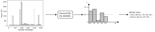
Figure 1: Classification of devices as active or inactive based on the household NILM data using classical ML or DL model to obtain $s_{i}$ for each device; devices with $s_{i}>0.5$ are classified as active, the others are classified as inactive.

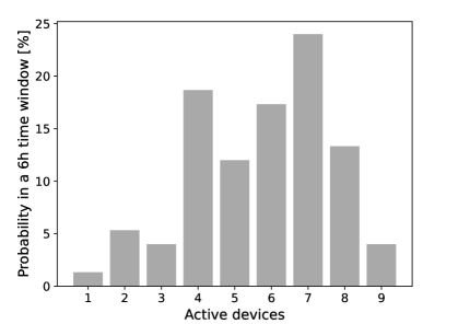
(a) REFIT

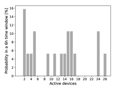
(b) UK-DALE

Figure 2: Probability distribution of the number of active devices in a 6 hours time window in REFIT and UK-DALE datasets.

I-B Contributions and Paper Organization

In this paper we are concerned with energy efficient ON/OFF classification of NILM data aimed at decreasing the overall energy consumption, which includes the investigation whether more complex and accurate DL approaches outweigh simpler and less consuming classical ML approaches. We propose a new DL architecture that is inspired by the VGG family of architectures and RNNs for the multi-label device activity classification on NILM data. We prove that its performance is better than state of the art CNNs and CRNNs and state of the art classical ML algorithms (RF), while being much more energy efficient compared to the state of the art DL models.

Based on the presented related work it can be seen that classical ML and DL models such as used in [16, 20, 25, 33, 34, 35, 36] and [37] are mostly tested in a way that is better suited for the comparison with other models and not in a way that would give realistic results of performance in real-world conditions.

To this end, this work examines a novel methodology that more accurately represents the performance of models in practical use cases. We approached the problem by first analysing the dataset to identify the number of active devices $N$ in the time window that the model is trained on. We then generated two distinct groups of mixed datasets, each comprising different sets of active and inactive devices. The first group contained mixed datasets with a fixed number of $N$ active devices, whereas the second group included mixed datasets with varying number of active devices between 1 and $N$. To generate the groups of mixed datasets we used REFIT [38] and UK-DALE [39] low-frequency datasets, also present in Tanoni et al. [16] and Langevin et al. [25].

Our main contributions are as follows:

• We propose a novel DL CtRNN architecture focusing on reduced computational complexity which offers superior performance compared to the existing state of the art architectures with an average improvement of approximately 8 percentage points on mixed datasets derived from REFIT and UK-DALE and more than 23 % lesser carbon footprint, making it a more sustainable solution.

• We propose a novel testing methodology that begins with a dataset analysis and involves generating two groups of mixed datasets that are utilized for both training and testing. By taking into account the unique properties of the original dataset when generating mixed datasets, our approach results in a more realistic evaluation of model performance, more closely reflecting real-world scenarios.

• We perform a comprehensive analysis taking into account performance and energy efficiency of compared approaches for NILM ON/OFF classification.

This paper is organized as follows. Sections I-A and  I-B describe related work and contributions, respectively. Section II provides the problem statement, Section III elaborates on methodological aspects, Section IV presents the proposed model and Section V provides a comprehensive evaluation. Finally, Section VI concludes the paper.

II Problem Statement

The objective of this study is to identify which devices are currently active using only the measurement of total electrical power $p(t)$, a process known as NILM. The total electrical power $p$ consumed by a household at any given moment $t$ is calculated as the sum of the power used by each electrical device, denoted as $p_{i}(t)$, where there are $N_{d}$ devices in total as defined in Eq. (1). Additionally, measurement noise (including any unidentified residual devices) $e(t)$ is also taken into account. The status indicator $s(t)$ determines the activity of each device, where $s(t)=0$ indicates that the device is inactive and $s(t)=1$ indicates that the device is active at the given moment $t$.

$$p(t)=\sum_{i=1}^{N_{d}}s_{i}(t)p_{i}(t)+e(t)$$ (1)

To solve the problem and thus estimate the status indicator $s_{i}(t)$ for each device, we can employ classical ML or DL for multi-label classification of devices. Devices are classified as active if the corresponding status indicator $s_{i}(t)$ predicted by the model exceeds 0.5, as illustrated in Figure 1. The cardinality of the set $s$ representing all the possible active devices, denoted by $|s|$, indicates the number of labels that need to be recognized. In the context of this paper, the value of $s$ varies between experiments as explained in Sections III-A and III-B.

III Methodology

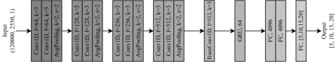
Figure 3: The proposed CtRNN architecture inspired by the VGG family of architectures.

We propose a methodology that aims to assess classical ML and DL models in a realistic scenario, which differs from the approaches commonly taken in recent works [16, 33, 34, 35, 36] and [37] that only use 5 distinct devices for evaluation. This limited number does not represent the typical diversity of devices encountered in real-world settings. For instance, the analysis of REFIT and UK-DALE datasets in Figure 2 reveals the presence of up to 9 and 26 active devices, respectively. Therefore, our methodology considers a wider range of devices for a more accurate evaluation of DL models in realistic conditions.

This methodology includes creating two groups of mixed datasets derived from REFIT and UK-DALE datasets, group A and group B, each containing multiple mixed datasets, designed to serve their specific purpose. Derivation of mixed datasets for group A and group B is explained more in detail in the following subsections.

III-A Group A

Group A is a group of multiple mixed datasets that cover cases where a fixed number of 5, 10, 15 or 20 devices in total (DiT) are in the household and 1, 2, …, $N_{max.AD}$ of them are active devices (AD). The number of DiT is used universally across all datasets and the maximum number of AD ($N_{max.AD}$) is used as a parameter depending on the maximum number of active devices in the time window that we are training our model on.

Group A datasets provide an insight into how the model in testing performs depending on the number of AD in four general cases of DiT, i.e. 5, 10, 15 and 20. In case of the UK-DALE dataset we also give an insight into a case of 54 DiT, which significantly exceeds the maximum number of DiT in the REFIT dataset.

In our case we were using 2550 samples for training, with sample rate of REFIT and UK-DALE that results in approximately 6 hour long time window. In the given time window there is a number of AD ranging from 1 to 9 for REFIT and from 2 to 26 for UK-DALE, as shown in Figure 2, thus $N_{max.AD}=9$ for REFIT and $N_{max.AD}=26$ for UK-DALE.

III-B Group B

Group B is a group of multiple mixed datasets that also cover cases where there are 5, 10, 15 and 20 DiT in the household, however we did not generate mixed datasets for different fixed number of AD but mixed datasets with an equal mix of all possible numbers of ADs. Thus, we generated 4 mixed datasets, each containing samples with 1, 2, …, $\overline{N_{max.AD}}$ ADs. Such group B presents more practical evaluation of the model by simulating a real-world scenario in which households utilize a variety of active devices rather than a fixed number.

In our case the average maximum number ($\overline{N_{max.AD}}$) of active devices was 8 for REFIT and 14 for UK-DALE. Therefore, the training data comprised time windows with ADs ranging from 1 to 8 and 1 to 14 for REFIT and UK-DALE, respectively. However, in cases where there were fewer devices in the household than active devices, the range of ADs was set to 1 to DiT-1. For instance, when there were 5 DiT in the household, the range of ADs was from 1 to 4, as was the case for both REFIT and UK-DALE datasets. Similarly, when there were 10 devices in the household, the range was from 1 to 9 ADs.

IV Proposed Neural Network Architecture

To achieve high classification performance, we introduce a new DL CRNN architecture, which was inspired by the VGG family of architectures but adapted for time series data and for lesser computation complexity and hence better energy efficiency. Our inspiration from VGG stems from the effectiveness of this type of architectures in NILM disaggregation [40].

The resulting architecture is illustrated in Figure 3, where each layer is clearly defined and explained in terms of its type and parameters. The architecture comprises four blocks, each consisting of two convolutional layers and one average pooling layer. The number of filters in each block doubles, starting from 64. Following the convolutional blocks, there is a transposed convolutional layer and a gated recurrent unit (GRU) layer. Prior to the output layer, there are two fully-connected layers with 4096 nodes. The number of nodes in the output layer is adjusted to meet the specific requirements and ranges from 5 to 54, depending on the used mixed dataset. All layers utilize the ReLU activation function, except for the output layer, which employs the sigmoid activation function.

The inclusion of a transposed convolutional layer in the proposed architecture draws inspiration from other state-of-the-art architectures [13, 14] developed for the purpose of ON/OFF classification on NILM. Moreover, the utilization of recurrent layers in state-of-the-art architectures [16, 25] has demonstrated notable performance benefits. In particular, the choice of employing the GRU layer was motivated by its usage in a study that closely aligns with our own research [16]. In order to enhance energy efficiency, we adhered to the principles derived from our prior work [28], we minimized the number of convolutional layers and replaced the fifth block of layers with a single transposed convolutional layer.

IV-A Computation Efficiency Considerations

As the purpose of using NILM is to reduce energy consumption, it is logical to ensure that the process itself is as energy-efficient as possible. Thus, our goal was to design a deep learning architecture that surpasses the state of the art not only in performance but also in terms of energy efficiency.

In order to assess the energy efficiency and carbon footprint of the architecture, it is necessary to calculate its complexity. This typically involves adding up the total number of FLOPs required for each layer.

We estimate the complexity of the most energy-consuming layers, namely the convolutional, pooling, and fully-connected layers, using the equations presented by Pirnat et al. in [28]. In addition, we calculate the complexity of the GRU layer using the equation proposed in [41].

We use equations from [28] to estimate the energy efficiency and carbon footprint of the proposed architecture and for comparison also for one popular reference architecture from the VGG family of architectures, i.e., VGG11, and for the two architectures used as a reference in performance evaluation, i.e., TanoniCRNN [16] and VAE-NILM [25]. This is done with an assumption that the architecture is trained and used on an Nvidia A100 graphics card and that each kWh of electricity produced results in 250g of CO₂ equivalent emissions (as it is the case for Slovenia).

Table II: Table of training parameters for CtRNN and VGG11, for group A on REFIT and UK-DALE (BS - batch size; LR - learning rate; E - no. of epochs).

CtRNN REFIT	1 AD			2 AD			3, 4 AD			5, 6, 7, 8 AD			9 AD
	BS	LR	E	BS	LR	E	BS	LR	E	BS	LR	E	BS	LR	E
5 DiT	512	$10^{-4}$	40	256	5$\times$$10^{-4}$	20	128	5$\times$$10^{-4}$	20	/	/	/	/	/	/
10 DiT	512	$10^{-4}$	40	256	5$\times$$10^{-4}$	20	128	5$\times$$10^{-4}$	20	128	5$\times$$10^{-4}$	20	128	$10^{-4}$	20
15 DiT	512	$10^{-4}$	40	256	5$\times$$10^{-4}$	20	128	5$\times$$10^{-4}$	20	128	5$\times$$10^{-4}$	20	128	5$\times$$10^{-4}$	20
20 DiT	512	$10^{-4}$	40	256	5$\times$$10^{-4}$	20	128	5$\times$$10^{-4}$	20	128	5$\times$$10^{-4}$	20	128	5$\times$$10^{-4}$	20
CtRNN UK-DALE	2, 3, 4 AD			5, 9 AD			11, 13 AD			14 AD			15, 16, 17 AD			24, 26 AD
	BS	LR	E	BS	LR	E	BS	LR	E	BS	LR	E	BS	LR	E	BS	LR	E
5 DiT	128	3$\times$$10^{-4}$	20	/	/	/	/	/	/	/	/	/	/	/	/	/	/	/
10 DiT	128	3$\times$$10^{-4}$	20	128	3$\times$$10^{-4}$	20	/	/	/	/	/	/	/	/	/	/	/	/
15 DiT	128	3$\times$$10^{-4}$	20	128	3$\times$$10^{-4}$	20	128	5$\times$$10^{-4}$	20	128	5$\times$$10^{-4}$	20	/	/	/	/	/	/
20 DiT	128	3$\times$$10^{-4}$	20	128	3$\times$$10^{-4}$	20	128	5$\times$$10^{-4}$	20	128	$10^{-4}$	20	128	$10^{-4}$	20	/	/	/
54 DiT	128	$10^{-4}$	20	128	$10^{-4}$	20	128	3$\times$$10^{-4}$	20	128	3$\times$$10^{-4}$	20	128	3$\times$$10^{-4}$	20	128	3$\times$$10^{-4}$	20
VGG11 REFIT	1 AD			2 AD			3, 4 AD			5, 6, 7, 8, 9 AD
	BS	LR	E	BS	LR	E	BS	LR	E	BS	LR	E
5 DiT	512	$10^{-4}$	50	256	$10^{-4}$	20	128	$10^{-4}$	20	/	/	/
10 DiT	512	$10^{-4}$	50	256	$10^{-4}$	20	128	$10^{-4}$	20	128	$10^{-4}$	20
15 DiT	512	$10^{-4}$	50	256	$10^{-4}$	20	128	$10^{-4}$	20	128	$10^{-4}$	20
20 DiT	512	$10^{-4}$	50	256	$10^{-4}$	20	128	$10^{-4}$	20	128	$10^{-4}$	20
VGG11 UK-DALE	2, 3, 4 AD			5, 9 AD			11, 13, 14 AD			16, 17			24, 26 AD
	BS	LR	E	BS	LR	E	BS	LR	E	BS	LR	E	BS	LR	E
5 DiT	128	$10^{-4}$	20	/	/	/	/	/	/	/	/	/	/	/	/
10 DiT	128	$10^{-4}$	20	128	$10^{-4}$	20	/	/	/	/	/	/	/	/	/
15 DiT	128	$10^{-4}$	20	128	$10^{-4}$	20	128	$10^{-4}$	20	/	/	/	/	/	/
20 DiT	128	$10^{-4}$	20	128	$10^{-4}$	20	128	$10^{-4}$	20	128	5$\times$$10^{-5}$	20	/	/	/
54 DiT	128	$10^{-4}$	20	128	$10^{-4}$	20	128	$10^{-4}$	20	128	5$\times$$10^{-5}$	20	128	5$\times$$10^{-5}$	20

IV-B Evaluation Datasets and Training Parameters

We first compared the performance of our model to VGG11 and with the performance of the model created by Tanoni et al. [16] adapted to fully supervised DL, and to results achieved by Langevin et al. [25], who were using the same dataset as we are. This comparison was done on the mixed dataset commonly used in recent works [16, 33, 34, 35, 36, 37]. It comprises a total of 5 devices, with each sample containing between 1 and 4 active devices selected at random. Samples with varying numbers of active devices are randomly interspersed throughout the mixed dataset. The 5 devices included in the mixed dataset are fridge, washing machine, dishwasher, microwave, and kettle, in line with recent research.

For this comparison we used a learning rate of 0.0003 and 20 epochs for our model while for the TanoniCRNN model we adopted the parameters specified as optimal in [16], which include the same number of epochs and a different learning rate of 0.002. Moreover, we used the same batch size of 128 for both models.

Subsequently we compared the performance of our model with that of VGG11 and RF on the two groups of mixed datasets A and B described in Section III. We choose VGG11 as a benchmark because VGG architectures are adopted in recent works [42, 43] for classification in NILM due to their effectiveness, and VGG11 is the closest match regarding the complexity. RF was chosen as the benchmark as it was reported to be the best algorithm for ON/OFF classification on NILM data in a previous study [11].

Training parameters used for group A are presented in Table II for CtRNN and VGG11 model. In summary, the batch size used for training both models was predominantly set to 128, with some variations of 256 or 512. The epoch count was set to 20 for both models in most cases, but it was also set to 50 for VGG11 and 40 for CtRNN, respectively, in certain scenarios. The learning rate ranged between $10^{-4}$ and $5\times 10^{-5}$ for VGG11 and between $5\times 10^{-4}$ and $5\times 10^{-5}$ for CtRNN.

Training parameters used for group B were simpler, always using batch size 128 and 20 epochs. Learning rate for CtRNN was 0.0003 on both REFIT and UK-DALE datasets; for VGG11 it was 0.0001 on both REFIT and UK-DALE datasets.

In all tests the batch size used is selected as the largest we could run or the one that gives the best results, selected through trial and error. It is equal for both models in the test as performance vary only slightly depending on its size.

Epochs and learning rate are tuned for performance and stability of the model through trial and error and may vary between the datasets, mixed datasets and models.

V Performance Evaluation

Using the proposed methodology with two groups of mixed datasets, we carried out comprehensive performance evaluation of CtRNN DL architecture and benchmarked it against selected state-of-the-art architectures in terms of energy efficiency and accuracy of determining the status of devices, as described in the following.

V-A Metrics

We evaluate the performance with a combined metric average weighted F1 score ($\overline{F1score_{w}}$), since performance evaluation based on a simple arithmetic mean of the F1 score would fail to provide an accurate reflection of the overall performance because our mixed datasets are generated in a way that does not provide each device equal representation. The use of weights ensures that all devices will affect the average score proportionally to how often they appear in the particular mixed dataset.

Average weighted F1 score is based on three metrics: true positive (TP), false positive (FP), and false negative (FN). TP represents the cases where the device is correctly classified as active, FP represents the cases where the device is incorrectly classified as active, and FN represents the cases where the device is incorrectly classified as inactive.

Using these metrics, we calculate the precision $Precision=\frac{TP}{TP+FP}$ and recall $Recall=\frac{TP}{TP+FN}$, and from these, we derive the F1 score $F1score=2\times\frac{Precision\times Recall}{Precision+Recall}$. To obtain the average weighted F1 score defined in Eq. (2), we calculate the F1 score for each device and then take the average based on their weight $Weight=\frac{SSD}{SAD}$, which is determined by the support for the specified device (SSD) and the support of all devices (SAD).

$$\overline{F1score_{w}}=\sum_{i=1}^{N_{d}}F1score_{i}\times Weight_{i}$$ (2)

Table III: CO₂ footprint used in training the proposed CtRNN model in comparison to VGG11, TanoniCRNN and VAE-NILM

NN	parameters	FLOPs	energy	carbon footprint
CtRNN	19.6 $\cdot\,10^{6}$	0.85 $\cdot\,10^{9}$	1510 kJ	104.9 g CO2 eq.
VGG11	185.6 $\cdot\,10^{6}$	1.21 $\cdot\,10^{9}$	2150 kJ	149.3 g CO2 eq.
TanoniCRNN [16]	0.75 $\cdot\,10^{6}$	1.11 $\cdot\,10^{9}$	1967 kJ	136.7 g CO2 eq.
VAE-NILM [25]	3.8 $\cdot\,10^{6}$	0.42 $\cdot\,10^{9}$	13.2 - 263 MJ	0.93 - 18.3 kg CO2 eq.

Table IV: Average weighted F1 score results for CtRNN compared to TanoniCRNN [16] and VAE-NILM [25] on mixed dataset of 5 devices derived from REFIT and UK-DALE.

devices	REFIT			UK-DALE
	CtRNN	Tanoni CRNN [16]	VAE-NILM [25]	CtRNN	Tanoni CRNN [16]	VAE-NILM [25]
fridge	0,93	0,92	0,85	1,0	1,0	0,81
washing machine	0,89	0,84	0,78	0,92	0,81	0,74
dish washer	0,88	0,80	0,84	0,87	0,86	0,65
microwave	0,89	0,71	0,59	0,96	0,80	0,32
kettle	0,95	0,87	0,87	0,93	0,86	0,87
weighted avg	0,91	0,83	0,78	0,94	0,87	0,68

V-B Energy Efficiency and Carbon Footprint

The results of our carbon footprint evaluation for training different architectures for each mixed dataset from group A or group B using batch size 128 are displayed in Table III. Despite TanoniCRNN having the lowest number of parameters, this does not result in lowest number of FLOPs, energy consumption and carbon footprint. Similarly, although VAE-NILM exhibits the lowest number of FLOPs, it has the highest energy consumption and carbon footprint. These factors are clearly influenced by additional training parameters, such as the number of epochs and batch size required to achieve satisfactory results. The proposed model outperforms state-of-the-art TanoniCRNN in terms of energy consumption and carbon footprint, with 23.3 % less carbon footprint produced on a mixed dataset tested on five commonly used devices. In addition, compared to VGG11 on groups A and B, the proposed model demonstrates 29.7 % less carbon footprint.

V-C Results on Mixed Dataset with 5 Commonly Used Devices

Comparison with Tanoni [16] and Langevin [25] on datasets of 5 devices derived from the REFIT and UK-DALE demonstrates superior performance of our proposed model with a significant gap in F1 score as can be seen in Table IV. Specifically, on the REFIT derived dataset, our model achieves a average weighted F1 score of 91 % compared to 83 % and 78 % obtained by TanoniCRNN and VAE-NILM, respectively, an improvement of 8 and 13 percentage points. On the UK-DALE derived dataset, our model outperforms TanoniCRNN and VAE-NILM by 7 and 26 percentage points, respectively, achieving an average weighted F1 score of 94 % compared to their 87 % and 68 %.

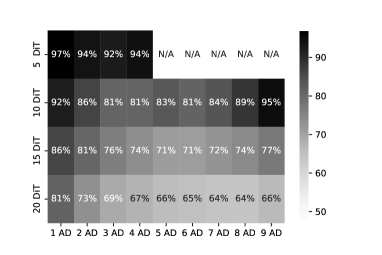
(a) REFIT CtRNN

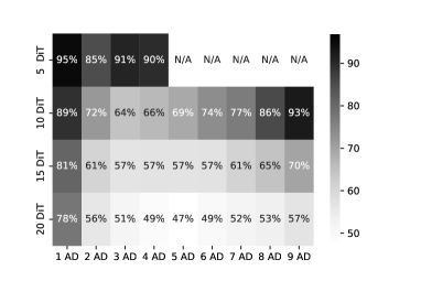
(b) REFIT VGG11

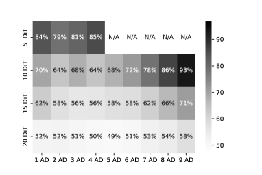
(c) REFIT RF

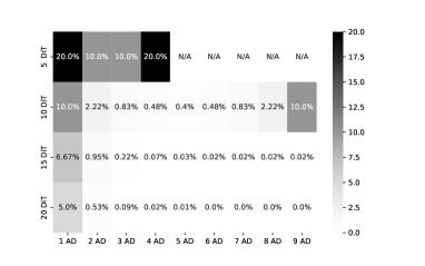
(d) REFIT Random

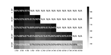
(e) UK-DALE CtRNN

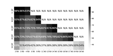
(f) UK-DALE VGG11

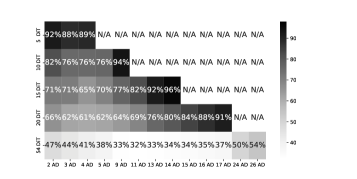
(g) UK-DALE RF

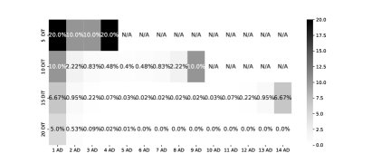
(h) UK-DALE Random

Figure 4: Results from RF, VGG11 and CtRNN on the group A of mixed datasets.

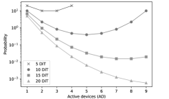
(a) REFIT

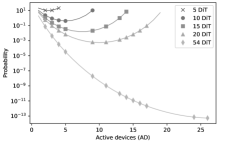
(b) UK-DALE

Figure 5: Probability of accurately determining the status (ON/OFF) of devices through random chance. The impact of this chance is reflected in the results of Test A, which are partially numerically aligned with these probability lines.

V-D Testing with Group A Mixed Datasets

The results of comparing the performance of CtRNN, VGG11 and RF models on group A mixed datasets are displayed in Figure 4. Subfigures a, b, and c exhibit heatmaps presenting the evaluation results of the models on the REFIT dataset, whereas subfigures e, f, and g depict heatmaps displaying the evaluation results on the UK-DALE dataset. Subfigures d and h, on the other hand, illustrate the probabilities of obtaining correct results randomly, calculated with Eq. 3.

$$P_{GroupA}=\frac{1}{\binom{DiT}{N_{AD}}}$$ (3)

The first observation shows that the accuracy of classification decreases with the increasing number of DiT and/or with the increasing number of active devices AD in the mixed dataset. The heatmaps’ cells can be compared to each other, for example on REFIT dataset in the row with 15 DiT our model achieves scores above 71 %, while models VGG11 and RF, achieve scores above 57 % and 56 %. All models outperform the random chance by a lot, as it reaches numbers as low as 0.02 %. To summarize the difference between the results of different models we calculated the average improvement (I) across all mixed datasets in group A, by aggregating the differences between the proposed CtRNN model and the compared model (X) on all datasets, and subsequently dividing by the total number of datasets ($N_{datasets}$), as expressed in Eq. (4):

Using Eq. (4), our model outperforms the VGG11 model by 11.03 and 9.4 percentage points on the REFIT and UK-DALE derived datasets, respectively. Compared to the RF model, our model achieves even greater improvement with 14.15 and 13.88 percentage points on the REFIT and UK-DALE derived datasets, respectively.

From the analysis of heatmaps in Figure 4 we notice a phenomenon, i.e., once the number of AD gets to 50 % or more of DiT in the mixed dataset the chance of correct classification increases. This phenomenon is clearly visible for both REFIT and UK-DALE in the lines with 5, 10 and 15 DiT and less so in the line with 20 DiT and for UK-DALE in the line with 54 DiT. To better understand the phenomenon we calculate random probability of correctly classifying devices in group A mixed datasets with Eq. 3 and depict the results in Figure 5. This improvement is at least in part caused by the probability of guessing the state of the device randomly, looking at the Figure 5 we notice similar decrease and increase in performance as previously seen in rows of the heatmaps in Figure 4.

REFIT				UK-DALE

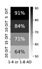
(a) CtRNN

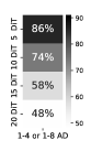
(b) VGG11

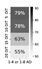
(c) RF

(d) Random

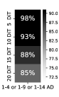
(e) CtRNN

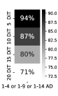
(f) VGG11

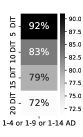
(g) RF

(h) Random

Figure 6: Results from RF, VGG11 and CtRNN on the group B of mixed datasets.

V-E Testing with Group B Mixed Datasets

The results of comparing the performance of CtRNN, VGG11 and RF models on group B mixed datasets are displayed in Figure 6. With the increase in DiT the accuracy of classification decreases in all cases. Random probability of correct classification, calculated by Eq. (5), much lower to the accuracy of the models, for example on REFIT dataset in row with 15 DiT our model achieves a score of 71 %, VGG11 achieves 58 % and RF achieves 63 %, whereas the random probability is rounded to 0 %.

$$P_{GroupB}=\frac{1}{2^{DiT}-\binom{DiT}{0}-\binom{DiT}{N_{AD}+1}-...-\binom{DiT}{DiT}}$$ (5)

We calculate the average improvement over the entire group B of mixed datasets using Eq. (4). Our model reaches results that are 11.32 percentage points better than VGG11 and 9.22 percentage points better than RF on REFIT derived dataset, and 8.07 percentage points better than VGG11 and 9.46 percentage points better than RF on UK-DALE derived dataset, respectively.

VI Conclusions

In this paper, we propose a new DL architecture CtRNN used in our models, paying special attention to improve its energy efficiency during training and operation as well as its performance compared to state of the art and other similar models. In developing the architecture, we used a typical VGG family architecture as a starting point and adapted it to time series data and reduced computational complexity by reducing the number of convolutional layers in some blocks, replacing one block with a single transposed convolution layer and adding the GRU layer. We benchmarked the proposed new model with other similar models, showing that it is possible to develop new DL models for NILM ON/OFF classification that provide a major improvement in both performance and energy efficiency, which results in lesser carbon footprint.

We also proposed a new methodology with two tests that more realistically assess the performance of NILM ON/OFF classification algorithms. They are using groups of multiple mixed datasets, derived from measurement datasets with specificities of the real-world use cases in mind. One group covers the numbers of active devices commonly used in the time window of the learning samples in separate datasets. The other group covers mixed number of devices from 1 to the average maximum number of devices used in the time window of the learning sample. Our findings demonstrate that the proposed methodology is necessary to obtain results, which reflect more realistic situations. The obtained results indicate that the commonly used testing methodology can lead to overly optimistic conclusions, underscoring the importance of employing a more rigorous evaluation framework. Moreover, as part of performance evaluation we also compared DL approaches and the best classical ML approach according to related work, and we concluded that DL approaches have a much higher performance potential compared to ML.

References

- [1] A. Q. Al-Shetwi, M. Hannan, K. P. Jern, M. Mansur, and T. Mahlia, “Grid-connected renewable energy sources: Review of the recent integration requirements and control methods,” Journal of Cleaner Production, vol. 253, p. 119831, 2020. [Online]. Available: https://www.sciencedirect.com/science/article/pii/S0959652619347018
- [2] J. Aghaei and M.-I. Alizadeh, “Demand response in smart electricity grids equipped with renewable energy sources: A review,” Renewable and Sustainable Energy Reviews, vol. 18, pp. 64–72, 2013. [Online]. Available: https://www.sciencedirect.com/science/article/pii/S1364032112005205
- [3] R. Gopinath, M. Kumar, C. Prakash Chandra Joshua, and K. Srinivas, “Energy management using non-intrusive load monitoring techniques – state-of-the-art and future research directions,” Sustainable Cities and Society, vol. 62, p. 102411, 2020. [Online]. Available: https://www.sciencedirect.com/science/article/pii/S2210670720306326
- [4] G. Hart, “Nonintrusive appliance load monitoring,” Proceedings of the IEEE, vol. 80, no. 12, pp. 1870–1891, 1992.
- [5] K. Ehrhardt-Martinez, K. A. Donnelly, S. Laitner et al., “Advanced metering initiatives and residential feedback programs: a meta-review for household electricity-saving opportunities,” in Advanced metering initiatives and residential feedback programs: a meta-review for household electricity-saving opportunities. American Council for an Energy-Efficient Economy Washington, DC, 2010.
- [6] A. Rahimpour, H. Qi, D. Fugate, and T. Kuruganti, “Non-intrusive energy disaggregation using non-negative matrix factorization with sum-to-k constraint,” IEEE Trans. on Power Systems, vol. 32, no. 6, pp. 4430–4441, 2017.
- [7] J. Kolter, S. Batra, and A. Ng, “Energy disaggregation via discriminative sparse coding,” Advances in neural information processing systems, vol. 23, 2010.
- [8] S. Singh and A. Majumdar, “Deep sparse coding for non–intrusive load monitoring,” IEEE Trans. on Smart Grid, vol. 9, no. 5, pp. 4669–4678, 2017.
- [9] M. Figueiredo, B. Ribeiro, and A. de Almeida, “Electrical signal source separation via nonnegative tensor factorization using on site measurements in a smart home,” IEEE Trans. on Instrumentation and Measurement, vol. 63, no. 2, pp. 364–373, 2013.
- [10] K. T. Chui, M. D. Lytras, and A. Visvizi, “Energy sustainability in smart cities: Artificial intelligence, smart monitoring, and optimization of energy consumption,” Energies, vol. 11, no. 11, p. 2869, 2018.
- [11] X. Wu, Y. Gao, and D. Jiao, “Multi-label classification based on random forest algorithm for non-intrusive load monitoring system,” Processes, vol. 7, no. 6, 2019. [Online]. Available: https://www.mdpi.com/2227-9717/7/6/337
- [12] B. Buddhahai, W. Wongseree, and P. Rakkwamsuk, “A non-intrusive load monitoring system using multi-label classification approach,” Sustainable Cities and Society, vol. 39, pp. 621–630, 2018. [Online]. Available: https://www.sciencedirect.com/science/article/pii/S2210670717315366
- [13] M. Zhou, S. Shao, X. Wang, Z. Zhu, and F. Hu, “Deep learning-based non-intrusive commercial load monitoring,” Sensors, vol. 22, no. 14, 2022. [Online]. Available: https://www.mdpi.com/1424-8220/22/14/5250
- [14] L. Massidda, M. Marrocu, and S. Manca, “Non-intrusive load disaggregation by convolutional neural network and multilabel classification,” Applied Sciences, vol. 10, no. 4, 2020. [Online]. Available: https://www.mdpi.com/2076-3417/10/4/1454
- [15] B. Bertalanič, J. Jenko, and C. Fortuna, “Dimensionality expansion of load monitoring time series and transfer learning for ems,” 2022. [Online]. Available: https://arxiv.org/abs/2204.02802
- [16] G. Tanoni, E. Principi, and S. Squartini, “Multi-label appliance classification with weakly labeled data for non-intrusive load monitoring,” IEEE Trans. on Smart Grid, pp. 1–1, 2022.
- [17] S. M. Tabatabaei, S. Dick, and W. Xu, “Toward non-intrusive load monitoring via multi-label classification,” IEEE Trans. on Smart Grid, vol. 8, no. 1, pp. 26–40, 2017.
- [18] G. A. Raiker, U. Loganathan, S. Agrawal, A. S. Thakur, K. Ashwin, J. P. Barton, M. Thomson et al., “Energy disaggregation using energy demand model and iot-based control,” IEEE Trans. on Industry Applications, vol. 57, no. 2, pp. 1746–1754, 2020.
- [19] S. Singh and A. Majumdar, “Non-intrusive load monitoring via multi-label sparse representation-based classification,” IEEE Trans. on Smart Grid, vol. 11, no. 2, pp. 1799–1801, 2020.
- [20] H. Çimen, E. J. Palacios-Garcia, N. Çetinkaya, J. C. Vasquez, and J. M. Guerrero, “A dual-input multi-label classification approach for non-intrusive load monitoring via deep learning,” in 2020 Zooming Innovation in Consumer Technologies Conference (ZINC), 2020, pp. 259–263.
- [21] F. Ciancetta, G. Bucci, E. Fiorucci, S. Mari, and A. Fioravanti, “A new convolutional neural network-based system for nilm applications,” IEEE Trans. on Instrumentation and Measurement, vol. 70, pp. 1–12, 2021.
- [22] J. Chen, X. Wang, X. Zhang, and W. Zhang, “Temporal and spectral feature learning with two-stream convolutional neural networks for appliance recognition in nilm,” IEEE Trans. on Smart Grid, vol. 13, no. 1, pp. 762–772, 2022.
- [23] Z. Zhou, Y. Xiang, H. Xu, Y. Wang, and D. Shi, “Unsupervised learning for non-intrusive load monitoring in smart grid based on spiking deep neural network,” Journal of Modern Power Systems and Clean Energy, vol. 10, no. 3, pp. 606–616, 2022.
- [24] H. Yin, K. Zhou, and S. Yang, “Non-intrusive load monitoring by load trajectory and multi feature based on dcnn,” IEEE Trans. on Industrial Informatics, pp. 1–12, 2023.
- [25] A. Langevin, M.-A. Carbonneau, M. Cheriet, and G. Gagnon, “Energy disaggregation using variational autoencoders,” Energy and Buildings, vol. 254, p. 111623, 2022. [Online]. Available: https://www.sciencedirect.com/science/article/pii/S0378778821009075
- [26] D. Li, K. Sawyer, and S. Dick, “Disaggregating household loads via semi-supervised multi-label classification,” in 2015 Annual Conf. of the North American Fuzzy Information Processing Society (NAFIPS), 2015, pp. 1–5.
- [27] M. A. A. Rehmani, S. Aslam, S. R. Tito, S. Soltic, P. Nieuwoudt, N. Pandey, and M. D. Ahmed, “Power profile and thresholding assisted multi-label nilm classification,” Energies, vol. 14, no. 22, 2021. [Online]. Available: https://www.mdpi.com/1996-1073/14/22/7609
- [28] A. Pirnat, B. Bertalanič, G. Cerar, M. Mohorčič, M. Meža, and C. Fortuna, “Towards sustainable deep learning for wireless fingerprinting localization,” in IEEE International Conference on Communications (ICC 2022), 2022, pp. 3208–3213.
- [29] M. A. Ahajjam, C. Essayeh, M. Ghogho, and A. Kobbane, “On multi-label classification for non-intrusive load identification using low sampling frequency datasets,” in 2021 IEEE International Instrumentation and Measurement Technology Conference (I2MTC), 2021, pp. 1–6.
- [30] G. Hsueh, Carbon Footprint of Machine Learning Algorithms. Senior Projects Spring 2020. 296., 2020. [Online]. Available: https://digitalcommons.bard.edu/senproj_s2020/296
- [31] M. Verhelst and B. Moons, “Embedded deep neural network processing: Algorithmic and processor techniques bring deep learning to iot and edge devices,” IEEE Solid-State Circuits Magazine, vol. 9, no. 4, pp. 55–65, 2017.
- [32] E. García-Martín, C. F. Rodrigues, G. Riley, and H. Grahn, “Estimation of energy consumption in machine learning,” Journal of Parallel and Distributed Computing, vol. 134, pp. 75–88, 2019. [Online]. Available: https://www.sciencedirect.com/science/article/pii/S0743731518308773
- [33] Y. Pan, K. Liu, Z. Shen, X. Cai, and Z. Jia, “Sequence-to-subsequence learning with conditional gan for power disaggregation,” in 2020 IEEE International Conf. on Acoustics, Speech and Signal Processing (ICASSP), 2020, pp. 3202–3206.
- [34] M. D’Incecco, S. Squartini, and M. Zhong, “Transfer learning for non-intrusive load monitoring,” IEEE Trans. on Smart Grid, vol. 11, no. 2, pp. 1419–1429, 2020.
- [35] L. Wang, S. Mao, B. M. Wilamowski, and R. M. Nelms, “Pre-trained models for non-intrusive appliance load monitoring,” IEEE Trans. on Green Communications and Networking, vol. 6, no. 1, pp. 56–68, 2022.
- [36] C. Zhang, M. Zhong, Z. Wang, N. Goddard, and C. Sutton, “Sequence-to-point learning with neural networks for non-intrusive load monitoring,” in 32nd AAAI Conf. on Artificial Intelligence (AAAI-18), 2018. [Online]. Available: https://ojs.aaai.org/index.php/AAAI/article/view/11873
- [37] J. Kelly and W. Knottenbelt, “Neural nilm: Deep neural networks applied to energy disaggregation,” in 2nd ACM international Conf. on embedded systems for energy-efficient built environments (BuildSys ’15), ser. BuildSys ’15. New York, NY, USA: Association for Computing Machinery, 2015, p. 55–64. [Online]. Available: https://doi.org/10.1145/2821650.2821672
- [38] D. Murray, L. Stankovic, and V. Stankovic, “An electrical load measurements dataset of united kingdom households from a two-year longitudinal study,” Scientific data, vol. 4, no. 1, pp. 1–12, 2017. [Online]. Available: https://doi.org/10.1038/sdata.2016.122
- [39] J. Kelly and W. Knottenbelt, “The uk-dale dataset, domestic appliance-level electricity demand and whole-house demand from five uk homes,” Scientific data, vol. 2, no. 1, pp. 1–14, 2015.
- [40] D. García-Pérez, D. Pérez-López, I. Díaz-Blanco, A. González-Muñiz, M. Domínguez-González, and A. A. Cuadrado Vega, “Fully-convolutional denoising auto-encoders for nilm in large non-residential buildings,” IEEE Trans. on Smart Grid, vol. 12, no. 3, pp. 2722–2731, 2021.
- [41] M. Zhang, W. Wang, X. Liu, J. Gao, and Y. He, “Navigating with graph representations for fast and scalable decoding of neural language models,” Advances in neural information processing systems, vol. 31, 2018.
- [42] W. Kong, Z. Y. Dong, B. Wang, J. Zhao, and J. Huang, “A practical solution for non-intrusive type ii load monitoring based on deep learning and post-processing,” IEEE Trans. on Smart Grid, vol. 11, no. 1, pp. 148–160, 2020.
- [43] D. Yang, X. Gao, L. Kong, Y. Pang, and B. Zhou, “An event-driven convolutional neural architecture for non-intrusive load monitoring of residential appliance,” IEEE Trans. on Consumer Electronics, vol. 66, no. 2, pp. 173–182, 2020.