Minimal graphs over non-compact domains in 3-manifolds with a Killing vector field

Abstract.

Let $\mathbb{E}$ be a connected and orientable Riemannian 3-manifold with a non-singular Killing vector field whose associated one-parameter group of the isometries of $\mathbb{E}$ acts freely and properly on $\mathbb{E}$. Then, there is a Killing submersion from $\mathbb{E}$ onto a connected and orientable surface $M$ whose fibers are the integral curves of the Killing vector field. In this setting we solve the Dirichlet problem for minimal Killing graphs over certain unbounded domains of $M$, taking piecewise continuous boundary values. We obtain general Collin-Krust type estimates. In the particular case of the Heisenberg group, we prove a uniqueness result for minimal Killing graphs with bounded boundary values over a strip. We also prove that isolated singularities of Killing graphs with prescribed mean curvature are removable.

1. Introduction

The Dirichlet problem for the mean curvature equation in unbounded domains has been extensively investigated over the past half-century, resulting in numerous advancements regarding the existence and uniqueness of solutions.

One of the earliest significant contributions in this field was made by H. Rosenberg and R. Sa Earp, [21]. They proved the existence of a solution to the Dirichlet problem for the minimal surface equation in unbounded domains that are contained in a strip or a sector of the plane.

Another pioneering work in this area was conducted by P. Collin and R. Krust, [5]. Their research focused on the Dirichlet problem for the prescribed mean curvature equation in Euclidean space, considering an unbounded domain $\Omega\subset\mathbb{R}^{2}$. The main theorem derived by Collin and Krust offers an asymptotic estimate of the difference between two solutions of this equation as these solutions approach infinity. This estimate serves as a vital tool in establishing the uniqueness of solutions.

To state the Collin–Krust result more precisely, it can be summarized as follows:

Theorem 1.1.

Let $\Omega\subset\mathbb{R}^{2}$ be an unbounded domain and let $u,\tilde{u}\in C^{2}(\Omega)$ be such that $u_{\mid\partial\Omega}=\tilde{u}_{\mid\partial\Omega}$ and

$$\mathop{\rm div}\nolimits\left(\frac{\nabla u}{\sqrt{1+\left\lVert{\nabla u}\right\rVert^{2}}}\right)=\mathop{\rm div}\nolimits\left(\frac{\nabla\tilde{u}}{\sqrt{1+\left\lVert{\nabla\tilde{u}}\right\rVert^{2}}}\right).$$

Denote $\Lambda(r)=\Omega\cap\left\{(x,y)\in\mathbb{R}^{2}:x^{2}+y^{2}=r\right\}$ and $M(r)=\underset{\Lambda(r)}{\sup}\,|u-\tilde{u}|$. Hence

$$\underset{r\to\infty}{\liminf}\frac{M(r)}{\ln r}>0.$$

Furthermore, if the length of $\Lambda(r)$ is uniformly bounded, then $\underset{r\to\infty}{\liminf}\frac{M(r)}{r}>0$.

The main purpose of this work is to extend the results in [21] and Theorem 1.1 to the more general setting of a Killing submersion. An oriented and connected 3-dimensional manifold $\mathbb{E}$ admitting a non-singular Killing vector field admits a Killing submersion $\pi:\mathbb{E}\to M$ onto a Riemannian surface $M$, connected and oriented, whose fibers are the integral curves of a non-zero Killing vector field $\xi\in\mathfrak{X}(\mathbb{E})$. This structure is a natural setting where we can study both the product 3-manifolds $M\times\mathbb{R}$ and the simply connected homogeneous 3-dimensional Riemannian manifold $\mathbb{E}$, whose space of Killing vector fields $\mathcal{K}(\mathbb{E})$ has dimension at least 3, and each $\xi\in\mathcal{K}(\mathbb{E})$ gives rise to a Killing submersion structure at points where $\mu=\left\lVert{\xi}\right\rVert>0$ (see [14, Examples 2.4, 2.5]).

The results originally established in [21] have been further expanded upon in subsequent works. In [22], R. Sa Earp and E. Toubiana extended these results to hyperbolic space, while in [23], they considered the case of $\mathbb{H}^{2}\times\mathbb{R}$. The authors, along with B. Nelli, further extended these findings to the Heisenberg group in [18]. In our work, we provide sufficient conditions that ensure the existence of a solution to the Dirichlet problem for the minimal surface equation in any Killing submersion over certain unbounded domains of $M$ that are asymptotically flat (see Theorem 3.3). Importantly, our approach distinguishes itself from previous works by not relying on the existence of supersolutions and subsolutions, which were necessary conditions in the proofs of earlier results.

Regarding Theorem 1.1, it has been extended to unitary Killing submersions by C. Leandro and H. Rosenberg in [13, Theorem 5.1], and improved in the specific case of minimal graphs in the three-dimensional Heisenberg group by J. M. Manzano and B. Nelli in [15, Theorem 7]. In all these results, the domain exhibits uniformly bounded or linear expansion, that is, there exists a positive constant $C$ such that either $\underset{r\to\infty}{\limsup}\mathop{\rm Length}\nolimits(\Lambda(r))\leq C$ or $\underset{r\to\infty}{\limsup}\tfrac{\mathop{\rm Length}\nolimits(\Lambda(r))}{r}\leq C$.

In Theorems 4.1 and 4.6, we provide a detailed description of the relationship between the growth of the vertical distance between two graphs with the same prescribed mean curvature and boundary values, and the rate of expansion of the domain where they are defined, without making any assumptions about the domain. Specifically, in Theorem 4.1, we show that the function $g(r)$, which describes the growth of the vertical distance, can be obtained by integrating the function $\tfrac{1}{\int_{\Lambda(r)}\mu^{2}}$. Building upon the ideas presented in [15, Theorem 7], in Theorem 4.6 we fix one of the two graphs and demonstrate that the growth function also depends on the area element of the fixed graph, which carries information about the bundle curvature $\tau$ and the prescribed mean curvature function $H$. Motivated by the examples, we believe that the hypotheses of Theorem 4.6 are sharp. In other words, when these hypotheses are not satisfied, it is possible to find two Killing graphs with the same boundary values and prescribed mean curvature that have a bounded vertical distance.

Utilizing these results, we prove the uniqueness of solutions to the Dirichlet problem for the minimal surface equation with bounded boundary values in a domain contained in a strip of $\mathbb{R}^{2}$ in the Heisenberg group (see Theorem 5.3 and Corollary 5.4). This provides a positive answer to two open questions posed in [18].

We also present additional results concerning graphs in Killing submersions. Firstly, we prove a removable singularity theorem for constant mean curvature (CMC) surfaces, extending the result found in [13, Theorem4.1] (see Theorem6.1). Additionally, we extend some of the results from this article to higher dimensions (see Theorems 7.3 and 7.4).

The paper is organized as follows. In Section 2, we describe the general properties and a local model for Killing submersions, we define the Killing graphs and recall their mean curvature equation and some existence results. In Section 3, we give sufficient conditions to prove the existence of minimal Killing graphs over unbounded domains $\Omega\subset M$. In Section 4, we prove the Collin-Krust type estimates. In Section 5, we restrict to the particular case of $\mathrm{Nil}_{3}$ and prove two uniqueness results in the strip. In Section 6, we generalize a removable singularity result proved by L. Bers [1] and R. Finn [12] in Euclidean space using the technique applied by C. Leandro and H. Rosenberg [13]. In Section 7, we prove a removable singularity theorem and a Collin-Krust type result for Killing submersions of arbitrary dimension.

2. Preliminaries and notation of Killing Submersions

In this section we recall some properties and results about Killing submersions. For further details we refer to [7, 8, 14].

Let $\pi\colon\mathbb{E}\to M$ be a Killing submersion with Killing vector field $\xi\in\mathfrak{X}(\mathbb{E})$. Assuming both $\mathbb{E}$ and $M$ simply connected, it was proven in [14, Theorems 2.6 and 2.9] that the metric of $\mathbb{E}$ is uniquely determined by the choice of $M$ and $\mu,\tau\in C^{\infty}(M).$ These geometric functions are the restriction to $M$ of the Killing length $\mu(p)=\left\lVert{\xi_{p}}\right\rVert$ and the bundle curvature $\tau(p)=\frac{-1}{\mu(p)}\langle\overline{\nabla}_{u}\xi,v\rangle$, where $\{u,v,\xi_{p}/\mu(p)\}$ is a positively oriented orthonormal basis of $T_{p}\mathbb{E}$ and $\overline{\nabla}$ denotes the Levi-Civita connection in $\mathbb{E}.$ Since both $\tau$ and $\mu$ are constant along the fibers they can be thought of as functions in $M.$ If $ds^{2}$ is the metric of $M$, we call $\mu$-metric the conformal metric $\mu^{2}ds^{2}$ and we will use the prefix “$\mu$” to indicate that the corresponding term is computed with respect to $\mu$-metric in $M$.

In this paper we will consider $M$ to be non-compact and the fibers of $\pi$ to have infinite length, which are natural assumptions for our results. Notice that the non-compactness of $M$ guarantees the existence of a global section ([14, Proposition 3.3]).

Denote by $\left\{\phi_{t}\right\}_{t\in\mathbb{R}}$ the one-parameter group of isometries associated to $\xi$. Let $\Omega\subseteq M$ be an open subset and let $F_{0}\colon\Omega\to\mathbb{E}$ be a smooth section. Hence the Killing graph of $u\in C^{\infty}(\Omega)$ with respect to $F_{0}$ is defined as the section of $\pi$ parameterized by the map

$$\begin{array}[]{rccc}F_{u}\colon&\Omega&\to&\mathbb{E}\\ &p&\mapsto&\phi_{u(p)}(F_{0}(p))\end{array}.$$

We recall some fundamental results about Killing graphs proved in [8]. In this setting the mean curvature of the graph of $u$ with respect to the section $F_{0}$ is given by the following formula:

$$H_{u}=\frac{1}{2\mu}\,\mathrm{div}(\mu\,\pi_{*}(N_{u}))=\frac{1}{2\mu}\,\mathrm{div}\left(\frac{\mu^{2}\,Gu}{\sqrt{1+\mu^{2}\|Gu\|^{2}}}\right).$$ (2.1)

Here $\mathrm{div}$ denotes the divergence on $M$ and $Gu=\nabla u-\pi_{*}(\overline{\nabla}d)$ is the so called generalized gradient, where $d\in\mathcal{C}^{\infty}(\mathbb{E})$ is the function such that $\phi_{d(p)}(F_{0}(\pi(p))=p$ for all $p\in\mathbb{E}.$ We denote $W_{u}=\sqrt{1+\mu^{2}\|Gu\|^{2}}$ the area element of $F_{u}$ and call angle function of $F_{u}$ the everywhere positive function

$$\nu=\langle N_{u},\xi\rangle=\frac{\mu}{W_{u}}.$$

The first result is a generalization of the technical lemma originally proved by R. Finn [12] in $\mathbb{R}^{3}$.

Lemma 2.1 ([8, Lemma 2.7]).

For any $u,v\in\mathcal{C}^{1}(M)$, let $N_{u}$ and $N_{v}$ be the upward-pointing unit normal vector fields to $F_{u}$ and $F_{v}$, respectively. Then

$$\left\langle\frac{Gu}{W_{u}}-\frac{Gv}{W_{v}},Gu-Gv\right\rangle=\frac{1}{2\mu^{2}}(W_{u}+W_{v})\|N_{u}-N_{v}\|^{2}\geq 0.$$

Equality holds at some point $q\in M$ if and only if $\nabla u(q)=\nabla v(q)$.

Finally, the following lemma provides a maximum principle for Killing graphs over compact domains of $M$.

Lemma 2.2 ([8, Proposition 4.2]).

Let $\Omega$ be a relatively compact open subset of $M$ with piecewise regular boundary. Let $u,v\in\mathcal{C}^{\infty}(\Omega)$ be functions that extend continuously to $\overline{\Omega}\setminus C,$ where $C\subset\partial\Omega$ is the finite set of non-continuity points of $u_{\mid\partial\Omega}$ and $v_{\mid\partial\Omega}$. If

• $H(u)\geq H(v)$ in $\Omega$ and

• $u\leq v$ in $\partial\Omega\setminus C$,

then $u\leq v$ in $\Omega$.

In the rest of the paper we will use assume that $p$ is a fixed point of $M$ and $\Omega\subset M$ is an unbounded domain. We denote by $B_{p}(r)$ the geodesic ball in $M$ centered at $p$ of radius $r$, $\Omega(r)=B_{p}(r)\cap\Omega$ and $\Lambda(r)=\partial B_{p}(r)\cap\Omega$. Given a curve $\gamma\subset M$, we denote by $\mathop{\rm Length}\nolimits(\gamma)$ the length of $\gamma$ computed with respect to the metric of $M$.

3. Existence of minimal Killing graphs over unbounded domains

In this section we prove the existence of minimal Killing graphs over certain unbounded domains of $M$ inspired by the ideas in [18].

First of all, we need to define in which kind of unbounded domains we are going to work.

Definition 3.1.

For $p\in M$ and $\alpha\in(0,2\pi)$ let $\tilde{W}$ be a wedge of angle $\alpha$ in $T_{p}M$. Then, if $\exp_{p}\colon\tilde{W}\to M$ is a diffeomorphism, we say that $W=\exp_{p}(\tilde{W})$ is a $\mu$-wedge of angle $\alpha$ and origin $p$.

Definition 3.2.

Let $\gamma_{1},\gamma_{2}\in M$ be two complete non-intersecting curves, both diffeomorphic to $\mathbb{R}$, such that $\gamma_{1}\cup\gamma_{2}$ is the boundary of a connected domain $S\subset M.$ We will say $S$ is a (convex) $\mu$-strip if the $\mu$-geodesic curvature of $\gamma_{1}\cup\gamma_{2}$ with respect to the inner normal pointing $S$ is non-negative.

We can now state the existence result as follows:

Theorem 3.3.

Let $\Omega\subset M$ be an unbounded $\mu$-convex domain contained either in a $\mu$-wedge $W$ of angle $\alpha<\pi$ or in a $\mu$-strip $S$ such that the $\mu$-metric of $M$ restricted to $W$ and $S$ is asymptotically flat. Let $\varphi$ be a function on $\partial\Omega$ continuous except at a discrete and closed set $U\subset\partial\Omega$ of points where $\varphi$ has finite left and right limits. Then there exists a minimal extension of $\varphi$ over $\bar{\Omega}$.

Proof.

The argument is inspired to the proof of [18, Theorem 4.3] and relies on the Compactness Theorem and on the existence of local barriers, that is guaranteed by the existence of solutions to the Jenkins–Serrin problem. In particular, the goal is to construct a sequence $\left\{u_{n}\right\}$ of minimal graph that will converge to the solution.

We study separately the the cases $\Omega\subseteq W$ and $\Omega\subseteq S.$

Case 1: $\Omega\subseteq W$. Let $p\in M$ the vertex of the $\mu$-wedge $W$ containing $\Omega$ and $\gamma_{1}(t)$ and $\gamma_{2}(t)$ be the two half $\mu$-geodesics parametrized by arc length such that $\gamma_{1}(0)=\gamma_{2}(0)=p$ and $\gamma_{1}(\mathbb{R}_{+})\cup\gamma_{2}(\mathbb{R}_{+})=\partial W$. For all $n\in\mathbb{N}$ sufficiently large, let $r_{n}=\gamma_{1}(n)$ and $s_{n}=\gamma_{2}(n)$ and $\gamma_{r_{n}}^{s_{n}}\subset W$ be the $\mu$-geodesic that joins $r_{n}$ and $s_{n}$ and is closest to $p.$ We denote by $T_{n}$ the $\mu$-geodesic triangle with vertices $p,\,r_{n}$ and $s_{n}$ such that $\gamma_{r_{n}}^{s_{n}}\subset\partial T_{n}$. Notice that there can be more then one such $\mu$-geodesic satisfying this hypothesis, but we can indistinctly choose one of them. With this choice for $\gamma_{r_{n}}^{s_{n}}$, any $\mu$-geodesic connecting $r_{n}$ and $s_{n}$ cannot lie in the interior of $T_{n}$.

We denote by $a_{n}$ (resp. $b_{n}$) the point of $\Omega\cap\gamma_{r_{n}}^{s_{n}}$ closest to $r_{n}$ (resp. $s_{n}$) and by $\Gamma_{n}$ the $\mu$-geodesic closest to $p$ joining $a_{n}$ and $b_{n}$ (notice that $\Gamma_{n}$ and $\gamma_{r_{n}}^{s_{n}}$ could be distinct). Finally we call $\Omega_{n}$ the domain bounded by $\partial\Omega\cap T_{n}$ and $\Gamma_{n}$ (see Figure 1).

Figure 1. Sequence of domains in the $\mu$-wedge

Since $U$ is discrete, we can assume that $\varphi$ is continuous at $a_{n}$ and $b_{n}$. Notice that, by construction, [8, Theorem 6.4] implies that in each $\Omega_{n}\neq\emptyset$ we can find a minimal graph $\omega_{n}^{\pm}$ such that $\omega_{n}^{\pm}=\varphi$ in $\partial\Omega\cap T_{n}$ and diverges to $\pm\infty$ approaching $\Gamma_{n}.$ Now we build a sequence of solution as in [18, Theorem 4.3]. On $\partial\Omega_{n}$, we consider a piecewise continuous function $\varphi_{n}$ such that it is continuous on $\Gamma_{n}$, with values between $\varphi(a_{n})$ and $\varphi(b_{n})$ and

$$\varphi_{n}(q)=\begin{cases}\begin{array}[]{lr}\varphi(q)&\textrm{if }q\in\partial\Omega_{n}\setminus\Gamma_{n};\\ \varphi(a_{n})&\textrm{if }q=a_{n};\\ \varphi(b_{n})&\textrm{if }q=b_{n}.\end{array}\end{cases}$$

As $\Omega_{n}$ is bounded and $\mu$-convex and $\varphi_{n}$ is piecewise continuous, [8, Theorem 6.4] guarantees the existence of a minimal extension $u_{n}$ of $\varphi_{n}$ on $\Omega_{n}$. We recall that for any discontinuity point $q\in\partial\Omega$, the boundary of the graph of each $u_{n}$ contains part of the fiber above $q$ with endpoints the left and the right limit of $\varphi$ at $q$. Moreover, there are no other points of the closure of the graph of $u_{n}$ on the vertical geodesic passing through the discontinuity points. Let $n_{0}$ be the smaller natural number such that $\Omega_{n_{0}}\neq\emptyset.$ The Maximum Principle implies that $\omega_{n_{0}}^{+}\geq u_{m}\geq\omega_{n_{0}}^{-}$ for all $m>n_{0}.$ Then, using the Compactness Theorem, we can take a subsequence $\left\{u_{n_{0},m}\right\}_{m}$ converging to a function $\tilde{u}_{n_{0}}$ in $\Omega_{n_{0}}.$ For any $n>n_{0}$, using $\omega_{n}^{+}$ and $\omega_{n}^{-}$ as barriers, we can solve the problem in $\Omega_{n}$ taking, by induction, a subsequence $\left\{u_{n,m}\right\}_{m}$ of $\left\{u_{n-1,m}\right\}_{m}$ converging to the function $\tilde{u}_{n}.$ By construction, $\tilde{u}_{m}=\tilde{u}_{n}$ in $\Omega_{n}$ for any $m>n$, that is, $\tilde{u}_{m}$ is the analytic extension of $\tilde{u}_{n}$ in $\Omega_{m}.$ Thus, $u=\lim_{n\to\infty}\tilde{u}_{u}$ will be the solution that we are looking for.

Case 2: $\Omega\subseteq S$. Let $\gamma_{1}(t)$ and $\gamma_{2}$ be the $\mu$-convex curves parametrized by arc length such that $\partial S=\gamma_{1}(\mathbb{R})\cup\gamma_{2}(\mathbb{R})$. For any $n>0$ we call $\eta_{n}^{l}\subset S$ (resp. $\eta_{n}^{r}\subset S$) the $\mu$-geodesic that minimizes the distance between $\gamma_{1}(-n)$ and $\gamma_{2}(-n)$ (resp. $\gamma_{1}(n)$ and $\gamma_{2}(n)$) and denote by $Q_{n}$ the quadrilateral domain bounded by $\gamma_{1}([-n,n])\cup\gamma_{1}([-n,n])\cup\eta_{n}^{l}\cup\eta_{n}^{r}.$ Let $a_{n}$ (resp. $d_{n}$) be the point in $\eta_{n}^{l}$ closest to $\gamma_{1}$ (resp. $\gamma_{2}$) and $b_{n}$ (resp. $c_{n}$) be the point in $\eta_{n}^{r}$ closest to $\gamma_{1}$ (resp. $\gamma_{2}$). We denote by $\Gamma_{n}^{l}$ (resp. $\Gamma_{n}^{r}$) the $\mu$-geodesic closest to $\eta_{n}^{l}$ (resp. $\eta_{n}^{l}$) joining $a_{n}$ and $d_{n}$ (resp. $b_{n}$ and $c_{n}$) and call $\Omega_{n}$ the domain bounded by $\Gamma_{n}=\Gamma_{n}^{l}\cup\Gamma_{n}^{r}$ and $\partial\Omega\cap Q_{n}$ (see Figure 2).

Figure 2. Sequence of domains in the $\mu$-strip

Since the $\mu$-metric in $S$ is asymptotically flat, there exist $n_{0}\in\mathbb{N}$ such that $\Omega_{n}$ satisfies the hypothesis of [8, Theorem 6.4] for any $n>n_{0}$. Therefore, there exist functions $\omega_{n}^{\pm}$ satisfying the minimal surface equation such that $\omega_{n}^{\pm}=\varphi$ in $\partial\Omega\cap Q_{n}$ and diverging to $\pm\infty$ as we approach $\Gamma_{n}.$

Now we can proceed as in the case of the wedge: since $U$ is discrete, without loss of generality, we can suppose that $\varphi$ is continuous at $a_{n},b_{n},c_{n},d_{n}$. On the boundary of $\Omega_{n}$, we consider a piecewise continuous function $\varphi_{n}$, continuous on $\Gamma_{n}^{l}$, with values between $\varphi(a_{n})$ and $\varphi(d_{n})$, and on $\Gamma_{n}^{r}$, with values between $\varphi(b_{n})$ and $\varphi(c_{n})$, such that

$$\varphi_{n}(q)=\begin{cases}\begin{array}[]{lr}\varphi(q)&\textrm{if }q\in\partial\Omega\cap Q_{n};\\ \varphi(a_{n})&\textrm{if }q=a_{n};\\ \varphi(b_{n})&\textrm{if }q=b_{n};\\ \varphi(c_{n})&\textrm{if }q=c_{n};\\ \varphi(d_{n})&\textrm{if }q=d_{n}.\end{array}\end{cases}$$

For any $n$ sufficiently large, we denote by $u_{n}$ the solution to the Dirichlet problem for minimal surface equation in $\Omega_{n}$ such that $u_{n}=\varphi_{n}$ in $\partial\Omega_{n}.$ By construction, for any $n,m\in\mathbb{N}$ with $m>n$, the Maximum Principle implies that $\omega_{n}^{+}\geq u_{m}\geq\omega_{n}^{-}$ in $\Omega_{n}.$ From this point on we can use the same argument as in Case 1 to conclude the proof. ∎

Remark 3.4.

Notice that, without assuming that the $\mu$-metric of $M$ restricted to $W$ (resp. $S$) is asymptotically flat, the sequence of $\mu$-geodesic triangles $T_{n}$ (resp $\mu$-quadrilaterals $Q_{n}$) satisfying the hypothesis of [8, Theorem 6.4] may not cover the $\mu$-wedge (resp. the $\mu$-strip).

Remark 3.5.

As in [18, Remark 4.4 (C)], if we assume $F_{0}$ to be minimal, when the boundary value $\varphi$ is bounded above (respectively below) by a constant $M$, then the solution given by our proof is also bounded above (respectively below) by the same constant $M$. Furthermore, if $\varphi$ is bounded both above and below, a global barrier is given by a vertical translation of $F_{0}$ and the solution that we find is bounded.

In general we can say nothing about the uniqueness of solutions in $\mu$-wedges and $\mu$-strips. In the forthcoming section, we will establish a Maximum Principle at infinity (see Theorems 4.1 and 4.6), which represents the initial step towards demonstrating the uniqueness of the solution of the Dirichlet problem over unbounded domains.

4. General Collin-Krust type results

This section is devoted to prove a result useful in the study of the uniqueness of a solution of the Dirichlet problem for the prescribed mean curvature equation over unbounded domains.

Let $\Omega\subset M$ be an unbounded domain and fix $p\in M$ such that $\Omega\cap\mathrm{Cut}(p)=\emptyset,$ this assumption will allows us to use the co-area formula. We denote by $B_{p}(r)$ the geodesic ball in $M$ centered at $p$ of radius $r$ and for any $r>r_{0}$ such that $\Omega(r)=B_{p}(r)\cap\Omega\neq\emptyset$ we call $\Lambda(r)=\partial B_{p}(r)\cap\Omega.$ The first result we prove provide an estimate of the growth of the difference of any two disjoint Killing graphs $u$ and $v$ over an unbounded domain $\Omega\subset M$, having the same prescribed mean curvature and boundary values. The theorem introduces three key functions: $M(r)$, $L(r)$, and $g(r)$;

• $M(r)$ measures the maximum difference between $u$ and $v$ over the region $\Lambda(r)$.

• $L(r)$ is defined as $\int_{\Lambda(r)}\mu^{2}$. This integral reflects the growth rate of the curve $\Lambda(r)$ with density $\mu$.

• $g(r)$ is defined as $\int_{r_{0}}^{r}\frac{ds}{L(s)}$ and measures the growth rate of $M(r)$.

The theorem states that if the function $g(r)$ tends to infinity as $r$ approaches infinity, the maximum difference between $u$ and $v$ over $\Lambda(r)$ grows at a rate that is at least comparable to the growth rate of $g(r)$.

In Theorem 4.6, we employ the idea presented in [15, Theorem 7] to improve the estimate of Theorem 4.1 when one of the two surfaces is known. Specifically, we consider one of the graphs as a fixed zero section of the Killing submersion. By doing so, we establish that the vertical growth of any Killing graph with zero boundary values and the same prescribed mean curvature $H_{0}$ as that of the zero section depends on the function $L(r)=\int_{\Lambda(r)}\frac{2\mu^{2}}{\sqrt{1+\mu^{2}(a^{2}+b^{2})}}$. Here, the smooth functions $a$ and $b$ defined in the domain $\Omega$ carry information regarding the bundle curvature $\tau$, as expressed in Equation (4.11), and the mean curvature of the zero section, as expressed in Equation (4.12).

Theorem 4.1.

Let $\Omega\subset M$ be an unbounded domain and assume that $p\in M$ is such that $\Omega\cap\mathrm{Cut}(p)=\emptyset.$ Assume also that $u,v\in\mathcal{C}^{\infty}(\Omega)$ satisfy $\mathcal{Q}(u)=\mathcal{Q}(v),$ $u>v$ in $\Omega$ and $u=v$ in $\partial\Omega.$ Let

$$M(r)=\underset{\Lambda(r)}{\sup}|u-v|,\qquad L(r)=\int_{\Lambda(r)}\mu^{2}\quad\textrm{ and }\quad g(r)=\int_{r_{0}}^{r}\tfrac{ds}{L(s)}$$

for some $r_{0}>0.$ Then,

$$\liminf_{r\to\infty}\frac{M(r)}{g(r)}>0.$$

Proof.

Denote by $\rho(r)=\int_{\Omega(r)}\left\lVert{\frac{\mu Gu}{W_{u}}-\frac{\mu Gv}{W_{v}}}\right\rVert^{2}$. The fact that $u-v>0$ in $\Omega$ implies that there exists $r_{0}>0$ such that $\rho(r_{0})>0$. Let us define $\eta(r)=\int_{\Lambda(r)}\mu\left\lVert{\frac{\mu Gu}{W_{u}}-\frac{\mu Gv}{W_{v}}}\right\rVert$, for all $r\geq r_{0}$. Using Lemma 2.1, the divergence theorem, and the fact that $\left\lVert{N_{u}-N_{v}}\right\rVert\geq\left\lVert{\frac{\mu Gu}{W_{u}}-\frac{\mu Gv}{W_{v}}}\right\rVert$, we can estimate for all $r\geq r_{0}$

$$\begin{array}[]{lcl}M(r)\eta(r)&\geq&\int_{\Lambda(r)}(u-v)\mu\left\lVert{\frac{\mu Gu}{W_{u}}-\frac{\mu Gv}{W_{v}}}\right\rVert=\int_{\partial\Omega(r)}(u-v)\mu\left\lVert{\frac{\mu Gu}{W_{u}}-\frac{\mu Gv}{W_{v}}}\right\rVert\\ &\geq&\int_{\partial\Omega(r)}(u-v)\left\langle{\frac{\mu^{2}Gu}{W_{u}}-\frac{\mu^{2}Gv}{W_{v}}},{\chi}\right\rangle\\ &=&\int_{\Omega(r)}\mathop{\rm div}\nolimits\left((u-v)\left(\frac{\mu^{2}Gu}{W_{u}}-\frac{\mu^{2}Gv}{W_{v}}\right)\right)\\ &=&\int_{\Omega(r)}\left\langle{\nabla u-\nabla v},{\frac{\mu^{2}Gu}{W_{u}}-\frac{\mu^{2}Gv}{W_{v}}}\right\rangle\\ &=&\int_{\Omega(r)}\frac{W_{u}+W_{v}}{2}\left\lVert{N_{u}-N_{v}}\right\rVert^{2}\\ &=&\rho(r_{0})+\int_{\Omega(r)\setminus\Omega(r_{0})}\frac{W_{u}+W_{v}}{2}\left\lVert{N_{u}-N_{v}}\right\rVert^{2}\\ &\overset{\text{(1)}}{\geq}&\rho(r_{0})+\int_{r_{0}}^{r}\left(\int_{\Lambda(s)}\left\lVert{\frac{\mu Gu}{W_{u}}-\frac{\mu Gv}{W_{v}}}\right\rVert^{2}\right)ds\\ &\overset{\text{(2)}}{\geq}&\rho(r_{0})+\int_{r_{0}}^{r}\frac{\eta^{2}(s)}{L(s)}ds,\end{array}$$ (4.1)

where $\chi$ denotes a unit co-normal vector field to $\Omega(r)$ along its boundary. The inequality (1) is a consequence of the co-area formula with respect to the Riemannian distance and (2) follows from the Cauchy-Schwarz inequality. Since $g(r)=\int_{r_{0}}^{r}\tfrac{ds}{L(s)},$ we get that

$$M(r)\eta(r)\geq\rho(r_{0})+\int_{r_{0}}^{r}g^{\prime}(s)\eta^{2}(s)ds$$ (4.2)

for all $r\geq r_{0}$.

The Maximum Principle implies that the function $r\mapsto M(r)$ does not decrease. Given $r_{1}>r_{0}$, let us write $a=M(r_{1})$, so $a\eta(r)\geq M(r)\eta(r)$ for all $r_{0}<r<r_{1}$. Hence, $\eta$ satisfies the integral inequality

$$\eta(r)\geq\frac{\rho(r_{0})}{a}+\frac{1}{a}\int_{r_{0}}^{r}g^{\prime}(s)\eta^{2}(s)ds.$$

Let us define the function $\zeta\colon[r_{0},R)\to\mathbb{R}$ as

$$\begin{array}[]{lcr}\zeta(r)=\frac{a\rho(r_{0})}{2a^{2}-\rho(r_{0})\left[g(r)-g(r_{0})\right]},\end{array}$$ (4.3)

where $R>r_{1}$ is defined as $R=g^{-1}\left(\frac{2a^{2}}{\rho(r_{0})}+g(r_{0})\right)$ if $\left(\frac{2a^{2}}{\rho(r_{0})}+g(r_{0})\right)\in\mathrm{Im}(g)$ and $R=+\infty$ otherwise. Observe that

$$\zeta^{\prime}(r)=\frac{a\rho(r_{0})g^{\prime}(r)}{(2a^{2}-\rho(r_{0})(g(r)-g(r_{0})))^{2}}=\tfrac{1}{a}\zeta(r)^{2}g^{\prime}(r),$$

whence

$$\zeta(r)=\frac{\rho(r_{0})}{2a}+\frac{1}{a}\int_{r_{0}}^{r}\zeta(s)^{2}g^{\prime}(s)ds.$$

Thus, a simple comparison yields $\eta\geq\zeta$ for all $r_{0}\leq r\leq r_{2}\leq R$, so that

$$\begin{array}[]{rl}r_{1}\leq r_{2}\iff&g(r_{1})\leq g(r_{2})\leq g(r_{0})+\tfrac{2a^{2}}{\rho(r_{0})}\\ \iff&2a^{2}\geq\rho(r_{0})\left(g(r_{1})-g(r_{0})\right)\\ \iff&a\geq\sqrt{\frac{\rho(r_{0})}{2}\left[g(r_{1})-g(r_{0})\right]},\textrm{ for all }r_{1}>r_{0}.\end{array}$$ (4.4)

We claim that the function $\eta$ is bounded away from zero at infinity. Note that, for $r>r_{0},$

$$\begin{array}[]{lcl}\eta(r)&\geq&\left|\int_{\Lambda(r)}\left\langle{\frac{\mu^{2}Gu}{W_{u}}-\frac{\mu^{2}Gv}{W_{v}}},{\chi}\right\rangle\right|\\ &\geq&\left|\int_{\partial\Omega(r)}\left\langle{\frac{\mu^{2}Gu}{W_{u}}-\frac{\mu^{2}Gv}{W_{v}}},{\chi}\right\rangle-\int_{\partial\Omega(r)\setminus\Lambda(r)}\left\langle{\frac{\mu^{2}Gu}{W_{u}}-\frac{\mu^{2}Gv}{W_{v}}},{\chi}\right\rangle\right|.\end{array}$$ (4.5)

The first integral of the right hand side of (4.5) vanishes by Stokes Theorem. So the result follows by proving that $\int_{\Gamma}\left\langle{\frac{\mu^{2}Gu}{W_{u}}-\frac{\mu^{2}Gv}{W_{v}}},{\chi}\right\rangle$ has constant sign on any arc $\Gamma$ contained in $\partial\Omega,$ as in [15]. Notice that $Gu-Gv=\nabla u-\nabla v\neq 0$ along $\partial\Omega$, except at isolated points, because $u-v\geq 0$ in $\Omega$ by assumption. In particular, $Gu-Gv$ is oriented toward $\Omega$, where it is not zero. Hence, $Gu-Gv$ can be used to orient $\partial\Omega$. Then, if $\mu^{2}\left\langle{\frac{Gu}{W_{u}}-\frac{Gv}{W_{v}}},{Gu-Gv}\right\rangle$ has constant sign along $\partial\Omega$, the same holds for $\left\langle{\mu^{2}\frac{Gu}{W_{u}}-\mu^{2}\frac{Gv}{W_{v}}},{\chi}\right\rangle$. By Lemma 2.1,

$$\mu^{2}\left\langle{\frac{Gu}{W_{u}}-\frac{Gv}{W_{v}}},{Gu-Gv}\right\rangle=\frac{1}{2}(W_{u}+W_{v})\left\lVert{N_{u}-N_{v}}\right\rVert^{2}$$

is positive at any point where $Gu-Gv$ is not zero. Then there exists a constant $n$ such that $\eta(r)\geq\int_{\Gamma}\mu^{2}\left\langle{\frac{Gu}{W_{u}}-\frac{Gv}{W_{v}}},{\chi}\right\rangle\geq n>0$, which proves the claim.

For any $r_{2}>r_{0}$, we deduce that

$$\begin{array}[]{ccl}\rho(r_{2})&=&\int_{\Omega(r_{2})}\left\lVert{\frac{\mu Gu}{W_{u}}-\frac{\mu Gv}{W_{v}}}\right\rVert^{2}\geq\int_{r_{0}}^{r_{2}}\left(\int_{\Lambda(s)}\left\lVert{\frac{\mu Gu}{W_{u}}-\frac{\mu Gv}{W_{v}}}\right\rVert^{2}\right)ds\\ &\geq&\int_{r_{0}}^{r_{2}}\frac{\eta^{2}(s)}{L(s)}ds\geq n^{2}\int_{r_{0}}^{r_{2}}g^{\prime}(s)ds\geq n^{2}\left[g(r_{2})-g(r_{0})\right].\end{array}$$ (4.6)

Observe that $g(r_{0})\leq\frac{g(r_{1})-g(r_{0})}{2}\leq g(r_{1}),$ so there is $r_{2}\in[r_{0},r_{1}]$ such that $g(r_{2})=\frac{g(r_{1})-g(r_{0})}{2}.$ Applying (4.4) to $r_{2}$ instead of $r_{0}$ we get

$$\begin{array}[]{rcl}M(r_{1})&\geq&\sqrt{\frac{\rho(r_{2})}{2}\left[g(r_{1})-g(r_{2})\right]}\geq\frac{n}{\sqrt{2}}\sqrt{\left[g(r_{1})-g(r_{2})\right]\left[g(r_{2})-g(r_{0})\right]}\\ &=&\frac{n}{2\sqrt{2}}\left[g(r_{1})-g(r_{0})\right]\end{array}$$ (4.7)

for all $r_{1}>r_{0}$. Finally, this means that

$$\liminf_{r\to\infty}\frac{M(r)}{g(r)}\geq\liminf_{r\to\infty}\left(\tfrac{n}{2\sqrt{2}}\left(1-\tfrac{g(r_{0})}{g(r)}\right)\right)>0$$

and this concludes the proof. ∎

Remark 4.2.

Up to lose some information, we can take

$$g(r)=\int_{r_{0}}^{r}\tfrac{ds}{T(s)^{2}\mathop{\rm Length}\nolimits(\Lambda(s))},$$

where $T(r)=\sup_{\Lambda(r)}\mu,$ to simplify the computation. Hence, if there exists a constant $C>0$ such that $\mu_{\mid\Omega}\leq C,$ then the growth function $g(r)$ will depend only on how the domain expands, that is $g^{\prime}(r)\geq\frac{1}{C^{2}\mathop{\rm Length}\nolimits(\Lambda(r))}.$

In the next example, when $\mu$ is bounded, we find a sharper bound on the growth of a domain $\Omega$ which guarantees a divergent Collin-Krust type estimate. Such domains exist, for instance, in $\mathbb{H}^{2}$ (see Figure 3).

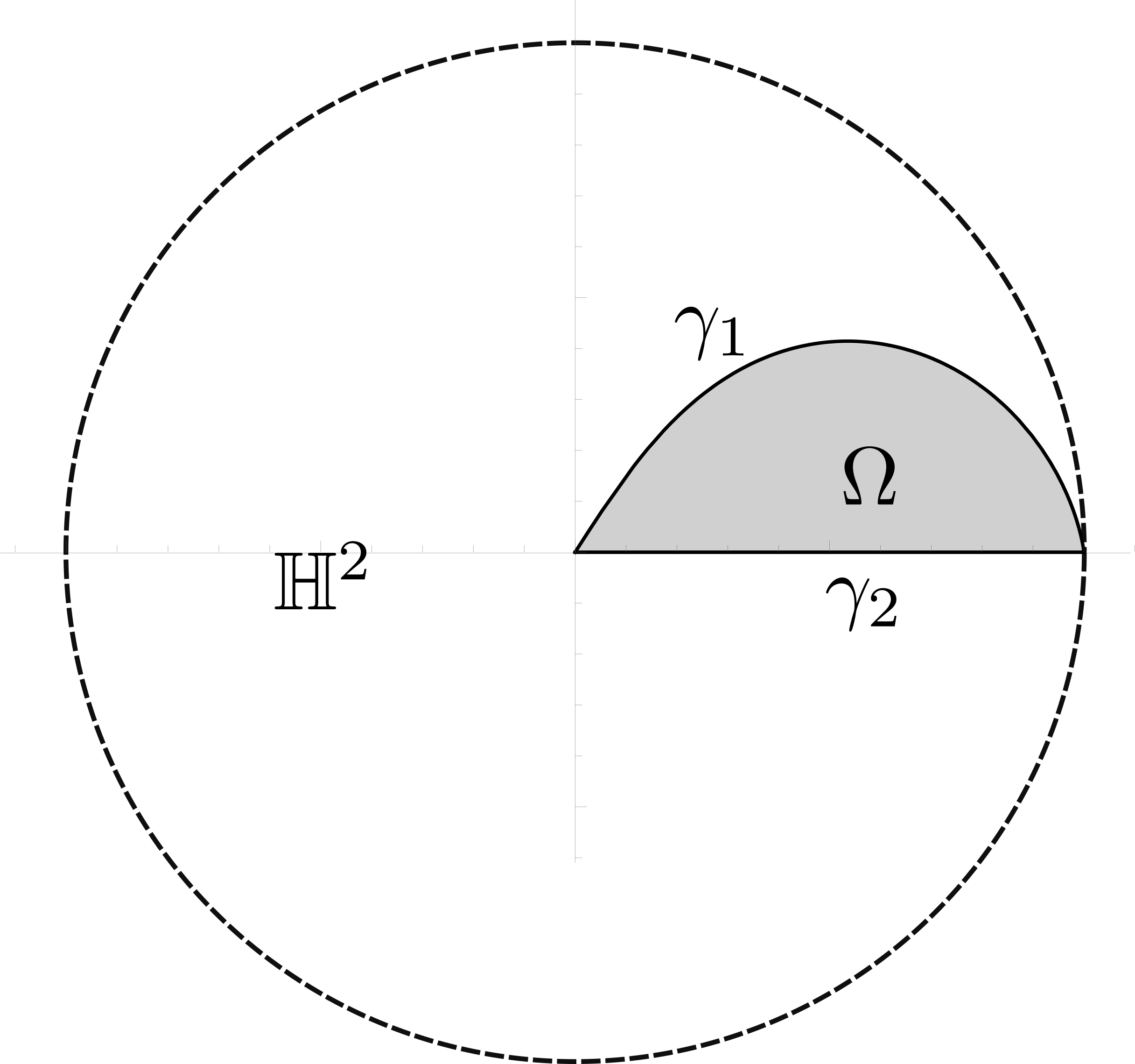
Figure 3. A domain in $\mathbb{H}^{2}$ whose expansion rate function is $(r+1)\log(r+1)$.

Using the Poincaré’s disk model, that is

$$\mathbb{H}^{2}=\left(\left\{(x,y)\in\mathbb{R}^{2}|x^{2}+y^{2}<1\right\},\frac{4}{(1-x^{2}-y^{2})^{2}}(dx^{2}+dy^{2})\right),$$

we can consider the convex domain $\Omega$ bounded by bounded by $\gamma_{1}\cup\gamma_{2}$, where $\gamma_{1},\gamma_{2}\colon[0,+\infty)\to\mathbb{H}^{2}$ are such that

$$\begin{array}[]{l}\gamma_{1}(t)=\left\{\tanh\left(\tfrac{t}{2}\right)\cos\left(\frac{(t+1)\log(t+1)}{\sinh(t)}\right),\tanh\left(\tfrac{t}{2}\right)\sin\left(\frac{(t+1)\log(t+1)}{\sinh(t)}\right)\right\},\\ \gamma_{2}(t)=\left\{\tanh\left(\tfrac{t}{2}\right),0\right\},\end{array}$$

which has expansion rate function $\mathop{\rm Length}\nolimits(\Lambda(r))=(r+1)\log(r+1)$.

Example 4.3.

It is not difficult to prove that $g(x)$ does not diverge whenever $f(x)=\frac{1}{g^{\prime}(r)}\geq cr(\log r)^{b+1}$ for some $b,c>0$, since

$$\int\frac{1}{cx(\log x)^{b+1}}dx=-\frac{1}{bc\left(\log x\right)^{b}}+cost,$$

which is bounded above. Nevertheless, we can build a sequence of monotone functions $\left\{f_{n}(x)\right\}_{n}$ such that, for all $n\geq 0,$

$$\underset{x\to+\infty}{\lim}\frac{f_{n+1}(x)}{f_{n}(x)}=+\infty,$$

and $\int\frac{1}{f_{n}(x)}$ diverges for $x\to+\infty$, with $f_{0}(x)=x$.

Define a sequence of function as follows:

$$\begin{cases}a_{0}(x)=x;\\ a_{i}(x)=\log(a_{i-1}(x))\qquad\textrm{for }i\geq 1.\end{cases}$$

Now we define $F_{n}(x)=\underset{i=0}{\overset{n}{\Pi}}a_{i}(x)$ and a sequence of translation terms

$$\begin{cases}x_{t}^{0}=0,\\ x_{t}^{i}=e^{x_{t}^{i-1}},\qquad\textrm{for all }i\geq 1.\end{cases}$$

Finally, we can define

$$f_{n}(x)=F_{n}(x+x_{t}^{n}).$$ (4.8)

It is easy to see that

$$g_{n}(x-x_{t}^{n+1})=\int\frac{1}{f_{n}(x-x_{t}^{n+1})}dx=\begin{cases}\begin{array}[]{ll}\tilde{a}_{0}(x)=\int\frac{1}{a_{0}(x)}dx&\textrm{for }n=0,\\ \tilde{a}_{n}(x)=\log(\tilde{a}_{n-1})&\textrm{for }n\geq 1,\end{array}\end{cases}$$

which diverges. Notice that the faster the domain expands, the smaller the growth function will be.

We now present an example where we construct two graphs with identical boundary values and mean curvature, while ensuring their vertical distance remains bounded. In particular, given the function describing the rate of expansion of $\Lambda(r)$, we are going to find for which choice of $\mu(r)$ the function $g(r)$, such that $g^{\prime}(r)=\frac{1}{L(r)}$, does not diverge for $r\to+\infty$ and then build a non-divergent minimal graph.

Example 4.4.

Let $\pi\colon\mathbb{E}\to M$ be a Killing submersion such that $M$ is the euclidean plane, $\tau\equiv 0$ and $\mu$ is a smooth radial function. We can consider in $\mathbb{R}^{2}$ the polar coordinates,

$$(\mathbb{R}^{2},g_{euc}=dx^{2}+dy^{2})\equiv\left(\mathbb{R}^{+}\times[0,2\pi),g_{pol}=dr^{2}+r^{2}d\theta\right).$$

We look for non-negative solutions $u$ defined in $\Omega=\left\{(r,\theta)\in\mathbb{R}\times[0,2\pi]\mid r\geq 1\right\}$ such that $u(1)=0$. It is easy to see that $u(r,\theta)=u(r)$ is a radial solution of the minimal surface equation in $\Omega$ if and only if $f(r)=\tfrac{\partial u}{\partial_{r}}(r)$ satisfies the following ODE:

$$\frac{\partial}{\partial r}\left(\frac{r\mu^{2}(r)f(r)}{\sqrt{1+\mu^{2}(r)f^{2}(r)}}\right)=0.$$ (4.9)

If $\mu(r,\theta)=r$, then the ODE becomes

$$\frac{\partial}{\partial r}\left(\frac{r^{3}f(r)}{\sqrt{1+r^{2}(r)f^{2}(r)}}\right)=0$$

Now, the solution is easy to compute: for all $c>1$,

$$f(r)=\frac{1}{\sqrt{cr^{6}-r^{2}}}.$$

Hence, $u\colon\Omega\to\mathbb{R}$ is given by

$$u(r)=\int_{1}^{r}\frac{ds}{\sqrt{cs^{6}-s^{2}}}=\frac{1}{2}\arctan\left(\sqrt{cr^{4}-1}\right)-\frac{1}{2}\arctan\left(\sqrt{c-1}\right).$$

First, notice that $u(r)$ is defined also for $c=1$ (this is the solution whose tangent at the boundary is vertical). Notice also that for $c\to+\infty$, the solutions $u(r)$ converge to $u(r)\equiv 0$. Finally, fixed $c\geq 1$,

$$0\leq\underset{r>1}{\sup}\,u(r)=\frac{\pi}{4}-\frac{1}{2}\arctan\left(\sqrt{c-1}\right)\leq\frac{\pi}{4}.$$

If $\mu(r,\theta)=\mu(r)$, the solution of (4.9) is the one-parameter family

$$u_{c}(r)=\pm\frac{1}{\sqrt{cr^{2}\mu(r)^{4}-\mu(r)^{2}}}=\pm\frac{1}{r\mu(r)^{2}\sqrt{c-\frac{1}{r^{2}\mu(r)^{2}}}},$$ (4.10)

depending on $c$. The comparison theorem for ODEs implies that, whenever $\mu(r)$ grows faster than $\log(r)^{\frac{a}{2}}$ with $a>1$, then

$$\underset{r\to+\infty}{\lim}\int_{r_{0}}^{r}u_{c}(s)ds<+\infty.$$

Hence, we can find two distinct minimal Killing graphs with the same boundary and bounded distance.

Taking $\mu(r)$ such that $\mu(r)^{2}_{\mid r\geq 2}=\log(r)$ and, using again the Comparison Theorem for ODEs, it is easy to see that the integral solution $u(r)=\int_{r_{0}}^{r}f_{c}(s)ds$ grows faster than $k\log(\log(r))$, for some constant $k>0$, which diverges. The same argument applies by taking $\mu(r)$ such that $r\mu^{2}(r)=f_{n}(x)$ for some $n>0$ where $\{f_{n}(x)\}_{n}$ is the sequence of function defined in (4.8). In particular, since $\mathop{\rm Length}\nolimits(\Lambda(r))=2\pi r,$ we obtain that the space can admit two Killing graph with the same mean curvature, the same boundary values and bounded difference, only if $\mu(r)$ grows faster than $\log(r)^{\frac{b}{2}}$ with $b>1$.

We can apply Theorem 4.1 to study when and how the difference between two Killing graphs in $\mathrm{Sol}_{3}$ with the same mean curvature and the same boundary values diverges. We want to show that, unlike in $\mathbb{H}^{2}\times\mathbb{R}$, in $\mathrm{Sol}_{3}$ there are some wedges where it makes sense to calculate a Collin–Krust type estimate.

Example 4.5.

The homogeneous manifold $\mathrm{Sol}_{3}$ is isometric to the warped product

$$\left(\left\{(x,y,z)\in\mathbb{R}^{3}\mid y>0\right\},\frac{dx^{2}+dy^{2}}{y^{2}}+y^{2}dz^{2}\right),$$

(see [19]). In this setting, it is easy to see that the function $u(x,y)=1-1/y$ defines a positive minimal graph in the unbounded domain of the hyperbolic plane $\left\{y>1\right\}$ that has zero boundary values and bounded height. Hence, in general, we can not expect to have a Collin–Krust type estimate in any domain.

Using the Mobius transformations, it easy to see that $\mathrm{Sol}_{3}$ is isometric to

$$\left(\mathbb{D}(1)\times\mathbb{R},ds^{2}=\frac{4(\mathrm{d}x^{2}+\mathrm{d}y^{2})}{(1-(x^{2}+y^{2}))^{2}}+\left(\frac{1-x^{2}-y^{2}}{(x-1)^{2}+y^{2}}\right)^{2}\mathrm{d}z^{2}\right).$$

That is, $\mathrm{Sol}_{3}$ is a Killing submersion over $\mathbb{H}^{2}$ (described with the Poincaré Disk Model) with $\tau\equiv 0$ and $\mu(x,y)=\frac{1-x^{2}-y^{2}}{(x-1)^{2}+y^{2}}$.

Let us define first in which kind of domain we want to compute the estimate. Let $\theta_{1},\theta_{2}\in(0,\pi)$ and for $t\in[0,1)$ define the geodesics $\gamma_{1}(t)=(t\cos\theta_{1},t\sin\theta_{1}$) and $\gamma_{2}(t)=(t\cos\theta_{2},-t\sin\theta_{2}$). We call $(\theta_{1},\theta_{2}$)-wedge the domain in $\mathbb{D}(1)$ bounded by $\gamma_{1}$, $\gamma_{2}$ and the asymptotic boundary $\gamma_{3}=(\cos\phi,\sin\phi),$ with $\phi\in(\theta_{1},2\pi-\theta_{2})$.

Figure 4. $(\theta_{1},\theta_{2})$-wedge.

Let $\Omega\subset\mathbb{H}^{2}$ be an unbounded domain contained in a $(\theta_{1},\theta_{2})$-wedge $W$ and $\Lambda(\rho)$ be the boundary of the geodesic ball of geodesic radius $\rho$ centered at the center of the Poincaré’s disk contained in $\Omega$. Thus $\mathop{\rm Length}\nolimits(\Lambda(\rho))\leq[2\pi-(\theta_{1}+\theta_{2})]\sinh(\rho)$ and

$$T(\rho)=\underset{\Lambda(\rho)}{\sup}\mu=\frac{1-\tanh(\rho)^{2}}{1+\tanh(\rho)^{2}-2\tanh(\rho)\cos(\theta)},$$

where $\theta=\min\left\{\theta_{1},\theta_{2}\right\}$. As explained in Theorem 4.1, $g=\int\frac{1}{\int_{\Lambda(r)}\mu^{2}},$ hence

$$\begin{array}[]{rl}g^{\prime}(\rho)\leq&\left(T^{2}(r)\mathop{\rm Length}\nolimits(\Lambda(r))\right)^{-1}=\frac{(1+\tanh(r)^{2}-2\tanh(r)\cos(\theta))^{2}}{[2\pi-(\theta_{1}+\theta_{2})]\sinh(r)[1-\tanh(r)^{2}]^{2}}.\end{array}$$

Integrating this inequality we have that

$$\begin{array}[]{rl}g(\rho)\leq&\frac{1}{2\pi-(\theta_{1}+\theta_{2})}\left[\tfrac{1}{2}\left(3+\cos(2\theta)\right)+\tfrac{1}{6}\left(2+\cos(2\theta)\right)\cosh(3r)\right.\\ &\left.+\log\left(\tanh\left(\tfrac{r}{2}\right)\right)-2\cos(\theta)\sinh(r)-\tfrac{2}{3}\cos(\theta)\sinh(3r)\right]\end{array}$$

which diverges whenever $\theta>0$.

Notice that, if $\Omega$ is an unbounded domain such that, for a $(\theta_{1},\theta_{2})$-wedge $W$, $\Omega\setminus W\neq\emptyset$ is compact and $u\in C^{\infty}(\Omega)$ describes a minimal Killing graph with bounded boundary values, then the positive (resp. negative) part of $u-\underset{\Omega\cap W}{\max}\,u$ (resp. $u+\underset{\Omega\cap W}{\min}\,u$) is a minimal Killing graph with zero boundary values over a non-compact domain contained in $W$ and we can apply the previous estimate.

To prove the last result of this section, we recall some details of the description of the local model of a Killing submersion. In [14], it was proven that $\mathbb{E}$ is locally isometric to $(\mathcal{U}\times\mathbb{R},ds^{2})$ where $\mathcal{U}\subseteq\mathbb{R}^{2}$ and $ds^{2}=\lambda^{2}(dx^{2}+dy^{2})+\mu^{2}[dz-\lambda(adx+bdy)]^{2}$ for some $\lambda,a,b\in C^{\infty}(\mathcal{U})$, with $\lambda>0$, such that $\left(\mathcal{U},\lambda^{2}(dx^{2}+dy^{2})\right)$ is a conformal parameterization of an unbounded and simply connected subset of $M$ and

$$\frac{2\tau}{\mu}=\frac{1}{\lambda^{2}}[(\lambda b)_{x}-(\lambda a)_{y}].$$ (4.11)

Equation (4.11) is the only condition on the choice of $a$ and $b$ to produce a Killing submersion with bundle curvature $\tau$ and Killing length $\mu$. Nevertheless, the choice of $a$ and $b$ affects the mean curvature of the section $z=0$, applying (2.1) to $u(x,y)\equiv 0$, it follows that:

$$H_{0}(x,y)=\frac{1}{2\mu}\left[\partial_{x}\left(\frac{\mu^{2}\lambda a}{\sqrt{1+\mu^{2}(a^{2}+b^{2})}}\right)+\partial_{y}\left(\frac{\mu^{2}\lambda b}{\sqrt{1+\mu^{2}(a^{2}+b^{2})}}\right)\right].$$ (4.12)

Furthermore, notice that if $d(x,y)$ is a $\mathcal{C}^{2}(\bar{\Omega})$ graph of mean curvature $H_{d}$, we can change $a,\,b$ for $\tilde{a},\,\tilde{b}$, where $\lambda(\tilde{a}-a)=d_{x}$ and $\lambda(\tilde{b}-b)=d_{y}$, and in this new model for $\mathbb{E}$ the section $z=0$ will have mean curvature $H_{0}=H_{d}$. (For further information about local coordinates in Killing submersions see [14, Section 2.1], [7, Section 2.2] and [8, Section 2.1]).In resume, the functions $a$ and $b$ depends on the bundle curvature $\tau$ of the ambient metric and on the mean curvature of the surface $\left\{z=0\right\}.$ Furthermore, it is easy to compute that the area elemente of $\left\{z=0\right\}$ is exactly $\sqrt{1+\mu^{2}(a^{2}+b^{2})}$. So, putting this information in (4.1), we can prove the following theorem.

Theorem 4.6.

Let $\Omega\subset M$ be an unbounded domain ad assume that $p\in M$ is such that $\Omega\cap\mathrm{Cut}(p)=\emptyset.$ Assume also that $u\in\mathcal{C}^{\infty}(\Omega)$ satisfy $H_{u}=H_{0},$ $u>0$ in $\Omega$ and $u=0$ in $\partial\Omega.$ Let

$$M(r)=\underset{\Lambda(r)}{\sup}|u-v|,\quad L(r)=\int_{\Lambda(r)}\frac{2\mu^{2}}{\sqrt{1+\mu^{2}(a^{2}+b^{2})}}\quad\textrm{ and }\quad g(r)=\int_{r_{0}}^{r}\tfrac{ds}{L(s)},$$

for some $r_{0}>0.$ Then,

$$\liminf_{r\to\infty}\frac{M(r)}{g(r)}>0.$$

Proof.

We do a slight modification of the proof of Theorem 4.1, starting from Equation (4.1). Then, recalling that $W_{u}\geq 1$ and $W_{0}=\sqrt{1+\mu^{2}(a^{2}+b^{2})}\geq 1$ we get

$$\begin{array}[]{lcl}M(r)\eta(r)&\geq&\int_{\Omega(r)}\frac{W_{u}+W_{0}}{2}\left\lVert{N_{u}-N_{0}}\right\rVert^{2}\\ &>&\rho+\int_{\Omega(r)\setminus\Omega(r_{0})}\frac{\sqrt{1+\mu^{2}(a^{2}+b^{2})}}{2}\left\lVert{\frac{\mu Gu}{W_{u}}-\frac{\mu Z}{W_{0}}}\right\rVert^{2}\\ &\overset{(1)}{\geq}&\rho+\int_{r_{0}}^{r}\left(\int_{\Lambda(s)}\frac{\sqrt{1+\mu^{2}(a^{2}+b^{2})}}{2}\left\lVert{\frac{\mu Gu}{W_{u}}-\frac{\mu Z}{W_{0}}}\right\rVert^{2}\right)ds\\ &\overset{(2)}{\geq}&\rho+\int_{r_{0}}^{r}\frac{\eta^{2}(s)}{L(s)}ds,\end{array}$$ (4.13)

where we have used the co-area formula in (1) and the Cauchy-Schwarz inequality in (2). From this point the argument is the same as the one in the proof of Theorem 4.1. ∎

To conclude this section, we show how Theorem 4.6 can be applied to the space $\mathbb{E}(-1,\tau)$, providing a better estimate than the one given in [13, Theorem 5.1]. In the case of unbounded domains where $\Lambda(\rho)$ is uniformly bounded, the result of Leandro and Rosenberg [13, Theorem 5.1] states that for every choice of $\tau$ and $H$, the distance between two surfaces which have the same mean curvature grows at least as $\rho$. We show that if $H=1/2$, the distance between two graphs having the same boundary values grows as $e^{\tfrac{\rho}{2}}$. We also show that, if we consider exterior domains, for any choice of $\tau$ and $H\in[0,1/2]$, the function $g(\rho)$ is not divergent.

Example 4.7.

Consider for $\mathbb{E}(-1,\tau)$ the global model given by

$$\left(\mathbb{D}(1)\times\mathbb{R},ds^{2}=\lambda^{2}(dx^{2}+dy^{2})+[2\tau\lambda(ydx-xdy)+dz]^{2}\right),$$

where $\lambda=\frac{2}{1-(x^{2}+y^{2})}$. In this model $a(x,y)=-2\tau y$ and $b(x,y)=2\tau x$. If we call $r=\sqrt{x^{2}+y^{2}}$, the geodesic distance of a point $(x,y)\in\mathbb{D}(1)$ from the center of the disk is given by $\rho=2\tanh^{-1}(r)$.

In [20], Peñafiel shows that an entire rotationally invariant graph of constant mean curvature $H\in[0,1/2]$ is $(\tanh(\rho/2)\cos\theta,\tanh(\rho/2)\sin\theta,u(\rho))$ where $u(\rho)$ satisfies

$$u^{\prime}(\rho)=\frac{\left(2H\cosh(\rho)-2H\right)\sqrt{1+4\tau^{2}\tanh^{2}(\rho/2)}}{\sqrt{\sinh^{2}(\rho)-(2H\cosh(\rho)-2H)^{2}}}.$$

Hence,

$$\tfrac{\partial}{\partial r}u(\rho(r))=u^{\prime}(\rho(r))\frac{\partial\rho}{\partial r}=\frac{4Hr\sqrt{1+4\tau^{2}r^{2}}}{(1-r^{2})\sqrt{1-4H^{2}r^{2}}}.$$

Now, in order to have an estimate for the vertical distance between an $H$-graph $\Sigma_{H}$ and the rotational entire $H$-graph $P_{H}$ described by Peñafiel, we have to compute

$$\tilde{a}(x,y)=\frac{u_{r}(\sqrt{x^{2}+y^{2}})}{\lambda}\frac{\partial r}{\partial x}+a(x,y),\quad \tilde{b}(x,y)=\frac{u_{r}(\sqrt{x^{2}+y^{2}})}{\lambda}\frac{\partial r}{\partial y}+b(x,y).$$

An easy computation implies,

$$\tilde{a}(x,y)=2Hx\sqrt{\frac{1+4\tau^{2}(x^{2}+y^{2})}{1-4H^{2}(x^{2}+y^{2})}}-2y\tau,$$

$$\tilde{b}(x,y)=2Hy\sqrt{\frac{1+4\tau^{2}(x^{2}+y^{2})}{1-4H^{2}(x^{2}+y^{2})}}+2x\tau.$$

Thus, defining

$$h(\rho)=(\tilde{a}^{2}+\tilde{b}^{2})(\rho)=\frac{4(H^{2}+\tau^{2})\tanh^{2}(\tfrac{\rho}{2})}{1-4H^{2}\tanh^{2}(\tfrac{\rho}{2})}$$

and $L(r)=\int_{\Lambda(r)}\tfrac{ds}{\sqrt{1+h(s)}}=\tfrac{2\mathop{\rm Length}\nolimits(\Lambda(r))}{1+h(\rho)}$, we have $g(\rho)=\int\frac{\sqrt{1+h(\rho)}}{2\mathop{\rm Length}\nolimits(\Lambda(r))}d\rho$.

Denoting by $\Omega\subset\mathbb{H}^{2}$ the domain bounded by $\pi(\Sigma_{H}\cap P_{H})$, our result shows that, if $\mathop{\rm Length}\nolimits(\Lambda(\rho))$ is uniformly bounded,

Figure 5. Domain in $\mathbb{H}^{2}$ such that $\Lambda(\rho)$ is uniformly bounded.

then $\Sigma_{H}-P_{H}$ grows as

$$g(r)\simeq\begin{cases}\begin{array}[]{ll}\left(\tfrac{1}{2}+\sqrt{\frac{H^{2}+\tau^{2}}{1-4H^{2}}}\right)r+o(r)&\textrm{for }0\leq H<\tfrac{1}{2};\\ &\\ \frac{\sqrt{1+4\tau^{2}}}{2}e^{\tfrac{r}{2}}+o\left(e^{\tfrac{r}{2}}\right)&\textrm{for }H=\tfrac{1}{2}.\end{array}\end{cases}$$

If $\Omega\subset\mathbb{H}^{2}$ is an exterior domain, then $\Lambda(r)\simeq 2\pi\sinh(r)$. Hence,

$$g^{\prime}(r)=\tfrac{1}{L(r)}\simeq\begin{cases}\begin{array}[]{ll}\sqrt{\frac{1-H^{2}-\tau^{2}}{4\pi^{2}(1-4H^{2})}}e^{-r}+o\left(e^{-r}\right)&\textrm{if }H,\tau\neq 0,\\ \sqrt{\frac{1+4\tau^{2}}{2\pi}}e^{-\tfrac{r}{2}}+o\left(e^{-\tfrac{r}{2}}\right)&\textrm{if }H=1/2.\end{array}\end{cases}$$

that is, $\underset{r\to\infty}{\lim}g(r)$ converges for any $0\leq H\leq 1/2$ an for any $\tau\in\mathbb{R}$. The existence of bounded graphs over exterior domains, characterized by zero boundary values and a constant mean curvature $H$ with respect to a rotational zero section of constant mean curvature $H$, has been established in various cases. Citti and Senni [2] demonstrated this existence for $\tau=0$ and $H\in(0,1/2)$. Peñafiel [20], focusing on surfaces invariant by rotation, proved the result for $H<1/2$ and any choice of $\tau$. In the work of Elbert, Nelli and Sa Earp [9], the case of $H=1/2$ and $\tau=0$ was proven. However, the existence of a similar result for $H=1/2$ and $\tau\neq 0$ remains unknown.

In all the examples we have seen, we were always able to find two different solutions whenever it was not possible to compute a generalized Collin-Krust estimate. So it seems natural to ask the following question:

• Assume that $\Omega\subset M$ is an unbounded domain such that for any choice of $p\in M,$ with $\Omega\cap\mathrm{Cut}(p)=\emptyset$, the function $g(r)=\int_{r_{0}}^{r}\tfrac{ds}{L(s)}$ does not diverge to $+\infty$. Does a positive and bounded solution to the following Dirichlet problem

  $$\begin{cases}\begin{array}[]{ll}\mathcal{Q}(u)=\mathcal{Q}(0)&\textrm{in }\Omega,\\ u=0&\textrm{in }\partial\Omega\end{array}\end{cases}$$

  exist?

5. A uniqueness results in a strip of the Heisenberg group

The 3-dimensional Heisenberg group is a particular case of Killing submersion where the base $M$ is $\mathbb{R}^{2}$ endowed with the Euclidean metric, $\mu\equiv 1$ and $\tau$ is constant. The classical model that describes $\mathrm{Nil}_{3}(\tau)$ is given by $\mathbb{R}^{3}$ endowed with the metric $ds^{2}=dx^{2}+dy^{2}+\left[\tau(ydx-xdy)+dz\right]^{2}$. In this model the Riemannian submersion reads as $\pi(x,y,z)=(x,y)$ and the Killing vector field is $\xi=\partial_{z}$.

In the Heisenberg space, Cartier constructed non-zero graphs over a wedge $\Omega\subset\mathbb{R}^{2}$ (with the vertex at the origin and any angle less the $\pi$) with zero values on $\partial\Omega$, which shows that the solution of the Dirichlet problem in $\Omega$ is not unique [3, Corollary 3.8]. We will prove an uniqueness result for minimal graphs with bounded boundary values over domains contained in a strip. The analogous problem was studied in $\mathbb{R}^{3}$ by Collin and Krust [5, Theorem 1] and by Elbert and Rosenberg in the product space $M\times\mathbb{R},$ [10, Theorem 1.1].

The ambient isometries of this model are generated by the following maps (see [11] for more details):

$$\begin{array}[]{ll}&\varphi_{1}^{c}(x,y,z)=(x+c,y,z+c\tau y),\\ &\varphi_{2}^{c}(x,y,z)=(x,y+c,z-c\tau x),\\ &\varphi_{3}^{c}(x,y,z)=(x,y,z+c),\\ &\varphi_{4}^{\theta}(x,y,z)=(x\cos\theta-y\sin\theta,x\sin\theta+y\cos\theta,z),\\ &\varphi_{5}(x,y,z)=(x,-y,-z).\\ \end{array}$$

For convenience, we will introduce the following notation. Let $\Omega\subseteq\mathbb{R}^{2}$ be an open subset and let $S\subset\mathrm{Nil}_{3}$ be the graph of a function $u^{S}\in\mathcal{C}^{2}(U)$ where $U\subset\mathbb{R}^{2}$ is an open subset containing $\overline{\Omega}.$ We call $P(S,\Omega)$ the following Dirichlet problem:

$$P(S,\Omega):\begin{cases}\begin{array}[]{lc}H_{u}=0&\textrm{in }\Omega,\\ u=u^{S}&\textrm{in }\partial\Omega.\end{array}\end{cases}$$

Let $\Omega$ be a domain contained in a strip of $\mathbb{R}^{2}.$ Without loss of generality, applying a rotation $\varphi_{4}^{\theta}$, we can assume $\Omega\subseteq\Omega_{a}^{b}=\left\{(x,y)\in\mathbb{R}^{2}\mid a<y<b\right\}$ for some $a,b\in\mathbb{R}$ such that $a<b$. Let $I\subset\mathrm{Nil}_{3}$ be the entire minimal graph invariant by $\varphi_{1}$ given by $u^{I}(x,y)=\tau xy.$

Lemma 5.1.

The only solution to $P(I,\Omega)$ is $u^{I}_{\mid\Omega}$.

Proof.

Let $c\in\mathbb{R}$ be such that $c>b-a$. Hence, [8, Theorem 6.4] implies that in the rectangle $R$ of vertices $A=(0,a)$, $B=(c,a)$, $C=(c,b)$ and $D=(0,b)$ there exists a unique minimal surface $\Sigma^{\pm}$, graph of the function $\omega^{\pm}$, intersecting the surface $I$ above the sides $\overline{AB}$ and $\overline{CD}$ and diverging to $\pm\infty$ over $\overline{BC}$ and $\overline{DA}$. If $u$ is any solution of $P(I,\Omega_{a}^{b}),$ it follows that $\omega^{-}\leq u\leq\omega^{+}$ in $\partial(\Omega_{a}^{b}\cap R)$, then the Maximum Principle implies that $\omega^{-}\leq u\leq\omega^{+}$ in $\Omega_{a}^{b}\cap R$ (see Figure 6).

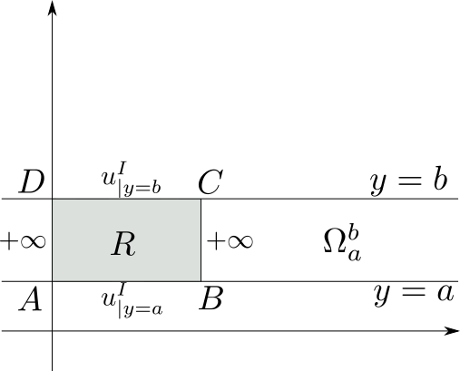
Figure 6. The upper barrier $\Sigma^{+}$.

Since $\varphi_{1}^{t}(I)=I$ and $\varphi_{1}^{t}$ is an isometry for all $t\in\mathbb{R},$ $\varphi_{1}^{t}(\Sigma^{+})$ (resp. $\varphi_{1}^{t}(\Sigma^{-})$) is above (resp. below) $I$ for all $t.$ It follows that there exists a positive constant $M$ such that any solution $\tilde{u}$ of $P(I,\Omega$) satisfies $|\tilde{u}(p)-u^{I}(p)|<M$ for all $p\in\Omega.$ However, Theorem 4.1 implies that $|\tilde{u}-u^{I}|$ is not bounded, so we are done. ∎

Remark 5.2.

Notice that, if $\Omega$ is a convex domain contained in a strip of $\mathbb{R}^{2}$, $f$ is a piecewise continuous function over $\partial\Omega,$ and there exists a positive constant $C$ such that $|u^{I}-f|<C$, then [18, Theorem 4.3] and Lemma 5.1 imply that there exists a unique minimal graph $u$ over $\Omega$ with $u_{\mid\partial\Omega}=f$ and $|u-u^{I}|<C$.

Using Lemma 5.1, it is easy to prove the following theorem, giving a positive answer to [18, Question (a), p.17].

Theorem 5.3.

The only minimal graph in $\mathrm{Nil}_{3}$ over a strip of $\mathbb{R}^{2}$ with zero values on the boundary of the strip is the trivial one.

Proof.

After applying a rotation $\varphi_{4}^{\theta}$ for some $\theta$, we consider the strip $\Omega_{a}^{b}$ parallel to the $x$-axis described above. For each $n\in\mathbb{N}$, denote by $R_{n}$ the rectangle of vertices $A_{n}=(-n,a)$, $B_{n}=(n,a)$, $C_{n}=(n,b)$ and $D_{n}=(-n,b)$. If $n_{0}>\frac{b-a}{2}$, [8, Theorem 6.4] guarantees that for any $n>n_{0}$ there exists a unique solution $\omega_{n}^{\pm}$ to the Jenkins–Serrin problem in $R_{n}$ that is zero on the sides parallel to the $x$-axis and diverges to $\pm\infty$ on the sides parallel to the $y$-axis. It is clear that, if $u$ is a minimal solution in $\Omega_{a}^{b}$ with zero boundary values, then $\omega_{n}^{+}>u>\omega_{n}^{-}$ for $n\in\mathbb{N}.$ Furthermore, for any $n>n_{0}$, the Maximum Principle implies that $\omega_{n-1}^{+}>\omega_{n}^{+}>0$ (resp. $\omega_{n-1}^{-}<\omega_{n}^{-}<0$) in $R_{n-1}$. Thus, the Compactness Theorem implies that the limit $\omega^{\pm}=\underset{n\to\infty}{\lim}\omega_{n}^{\pm}$ exist and we call $\Sigma^{\pm}$ their graphs.

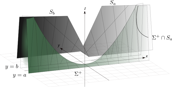
Figure 7. A contradiction on the growth of $\omega^{+}$.

If $\omega^{+}\equiv 0\equiv\omega^{-}$, then we are done. So, suppose for instance that $\omega^{+}\neq 0$ in $\Omega_{a}^{b}$ (the same argument can be applied with a slight modification to $\omega^{-}$). Theorem 4.6 implies that $\omega^{+}$ has a quadratic height growth. We first study the asymptotic behaviour of $\omega^{+}$ in $\Omega_{a}^{b}\cap\left\{x\geq 0\right\}$. Let

$$M=\sup_{y\in(a,b)}\omega_{n_{0}}^{+}(0,y)$$

and, for any $c\in\mathbb{R}$, denote by $S=\varphi_{2}^{c/2}(I)$ (that is, the graph of the function $u(x,y)=\tau x(y-c)$), and $S_{c}=\varphi_{3}^{M}(S)$ (that is, the graph of $u_{c}(x,y)=M+\tau x(y-c)$). Thus, by construction, $u_{a}\geq\omega^{+}$ in $\partial(\Omega_{a}^{b}\cap\left\{x\geq 0\right\})$. Since $u_{a}$ has a linear height growth, it follows that

$$\Omega=\left\{(x,y)\in\Omega_{a}^{b}\mid x\geq 0,u_{a}(x,y)<\omega^{+}(x,y)\right\}\neq\emptyset.$$

Hence, $\omega^{+}_{\mid\Omega}\neq u_{a}$ is a solution of $P(S_{a},\Omega)$ in contradiction with Lemma 5.1. To study the behaviour of $\omega^{+}$ in $\Omega_{a}^{b}\cap\left\{x\geq 0\right\}$, we apply the same argument by replacing $S_{a}$ with $S_{b}$. ∎

Once we have proved that the only minimal solution with constant boundary values on a strip is the constant one, we can give a positive answer to [18, Question (b), p.17].

Corollary 5.4.

Let $\Omega$ be a domain contained in a strip of $\mathbb{R}^{2}$ and $\phi\colon\partial\Omega\to\mathbb{R}$ be a piecewise $\mathcal{C}^{2}$-function and suppose that there exists $m,M\in\mathbb{R}$ such that $m<\phi<M$. Hence the solution to the problem

$$\begin{cases}\begin{array}[]{lc}H_{u}=0&\textrm{in }\Omega,\\ u=\phi&\textrm{in }\partial\Omega\end{array}\end{cases}$$

is unique and satisfies $m<u<M$.

Remark 5.5.

It is possible to study the problem of uniqueness of minimal graphs in a strip of $\widetilde{\mathrm{SL}}_{2}(\mathbb{R})$, as a Killing submersion over $\mathbb{H}^{2}$ with $\mu\equiv 1$ and $\tau$ constant, that can be described as $\left\{\mathbb{D}\times\mathbb{R},ds^{2}\right\}$, with $\mathbb{D}=\left\{(x,y)\in\mathbb{R}^{2}\mid\lambda(x,y)>0\right\}$ and $ds^{2}=\lambda^{2}(dx^{2}+dy^{2})+\left[2\tau\lambda(ydx-xdy)+dz\right]^{2}$,where $\lambda=\frac{2}{1-(x^{2}+y^{2})}$. In this context $\varphi_{1}$ should be defined as the lifting of hyperbolic translation, so it makes sense to consider a strip invariant by an hyperbolic translation, i.e., the non-compact domain whose boundary is the union of two complete curves which are equidistant from a fixed geodesic. The minimal graphs invariant by $\varphi_{1}$ in $\widetilde{\mathrm{SL}}_{2}(\mathbb{R})$ have bounded height (see for example [4] or [20]), so the arguments used for $\mathrm{Nil}_{3}$ can be easily adapted to this case.

6. Removable singularities Theorem

In this section we prove a removable singularity result firstly proved by L. Bers [1] for minimal graphs, then by Finn [12] for graphs of prescribed mean curvature in $\mathbb{R}^{3}$, by Nelli and Sa Earp[17] for graphs of prescribed mean curvature in the hyperbolic space and then extended in unitary Killing submersions by C. Leandro and H. Rosenberg [13, Theorem 4.1]. The same technique used in [13] can be applied since the function $\mu$ has an upper bound in the domains of $M$ where we are working. This extension guarantees a removable singularity result, for example, in $\mathrm{Sol}_{3}$ and for rotational graphs in $\mathbb{R}^{3}$.

Theorem 6.1.

Let $u\colon\Omega\setminus\left\{p\right\}\to\mathbb{R}$, $\Omega\subset M$, be a function whose Killing graph has prescribed mean curvature $H\in C^{0,\alpha}(\overline{\Omega})$. Then $u$ extends smoothly to a solution at $p$.

Proof.

For any $R>0$, denote by $B_{R}(p)$ the $\mu$-geodesic ball geodesic of radius $R$ centered in $p\in M$. If $R$ is sufficiently small, [6, Theorem 1] guarantees the existence of a smooth function $v$ defined on $B_{R}(p)$ with:

$$\begin{cases}\begin{array}[]{ll}\mathop{\rm div}\nolimits\left(\frac{\mu^{2}Gv}{W_{v}}\right)=2\mu H,&\textrm{in }B_{R}(p);\\ v=u,&\textrm{in }\partial B_{R}(p).\end{array}\end{cases}$$

Fix a positive constant $C$ and define the Lipschitz function

$$\varphi=\begin{cases}\begin{array}[]{ll}u-v,&\textrm{if }\mid u-v\mid\ <C;\\ C,&\textrm{if }\mid u-v\mid\geq C.\end{array}\end{cases}$$

By definition, $\varphi$ satisfies $\nabla\varphi=\nabla u-\nabla v=Gu-Gv$ in the set $\mid u-v\mid<C$ and $\nabla\varphi=0$ in its complement.

For $0<r<R$, let $A(r,R)=B_{R}(p)\setminus B_{r}(p)$ and denote by $m=\underset{\tiny B_{R}(p)}{\max}\mu$. Hence,

$$\begin{array}[]{rcl}\int_{\partial A(r,R)}\varphi\mu\left\langle{\frac{\mu Gu}{W_{u}}-\frac{\mu Gv}{W_{v}},\nu}\right\rangle&=&\int_{\partial B_{r}(p)}\varphi\mu\left\langle{\frac{\mu Gu}{W_{u}}-\frac{\mu Gv}{W_{v}},\nu}\right\rangle+\int_{\partial B_{R}(p)}\varphi\mu\left\langle{\frac{\mu Gu}{W_{u}}-\frac{\mu Gv}{W_{v}},\nu}\right\rangle\\ &\leq&\int_{\partial B_{r}(p)}Cm=Cm\mathop{\rm Length}\nolimits(\partial B_{r}(p)).\end{array}$$

Since the Killing graphs of $u$ and $v$ have the same mean curvature, we have that, when $\mid u-v\mid\geq C$, $\mathop{\rm div}\nolimits\varphi\left(\frac{\mu^{2}Gu}{W_{u}}-\frac{\mu^{2}Gv}{W_{v}}\right)=0$ and, when $\mid u-v\mid<C$,

$$\begin{array}[]{rl}\mathop{\rm div}\nolimits\varphi\left(\frac{\mu^{2}Gu}{W_{u}}-\frac{\mu^{2}Gv}{W_{v}}\right)=&\left\langle{\nabla\varphi,\frac{\mu^{2}Gu}{W_{u}}-\frac{\mu^{2}Gv}{W_{v}}}\right\rangle+\varphi\mathop{\rm div}\nolimits\left(\frac{\mu^{2}Gu}{W_{u}}-\frac{\mu^{2}Gv}{W_{v}}\right)\\ =&\left\langle{\nabla\varphi,\frac{\mu^{2}Gu}{W_{u}}-\frac{\mu^{2}Gv}{W_{v}}}\right\rangle\\ =&\left\langle{\nabla u-\nabla v,\frac{\mu^{2}Gu}{W_{u}}-\frac{\mu^{2}Gv}{W_{v}}}\right\rangle\\ =&\left\langle{Gu-Gv,\frac{\mu^{2}Gu}{W_{u}}-\frac{\mu^{2}Gv}{W_{v}}}\right\rangle\\ =&\frac{W_{u}+W_{v}}{2}\left\lVert{N_{u}-N_{v}}\right\rVert^{2}_{\mathbb{E}}\leq\left\lVert{N_{u}-N_{v}}\right\rVert^{2}_{\mathbb{E}},\end{array}$$

where the last equality follows by Lemma 2.1. By Stokes Theorem, we have

$$\begin{array}[]{c}\int_{A(r,R)}\mathop{\rm div}\nolimits\varphi\left(\frac{\mu^{2}Gu}{W_{u}}-\frac{\mu^{2}Gv}{W_{v}}\right)=\int_{\partial A(r,R)}\varphi\left\langle{\frac{\mu^{2}Gu}{W_{u}}-\frac{\mu^{2}Gv}{W_{v}},\nu}\right\rangle\\ =\int_{\partial A(r,R)}\varphi\mu\left\langle{\frac{\mu Gu}{W_{u}}-\frac{\mu Gv}{W_{v}},\nu}\right\rangle\leq Cm\mathop{\rm Length}\nolimits(S_{r}).\end{array}$$ (6.1)

Thus, it follows that

$$0\leq\int_{A(r,R)\cap\left\{\mid u-v\mid<C\right\}}\left\lVert{N_{u}-N_{v}}\right\rVert^{2}_{\mathbb{E}}\leq Cm\mathop{\rm Length}\nolimits(S_{r}).$$

Since $m$ does not depend on $r$, as $r$ decreases to zero we get that $N_{u}=N_{v}$ on the set $|u-v|<C$. Hence $Gu=Gv$ in the set $\mid u-v\mid<C$. Since $C$ was arbitrary, we have that $Gu=Gv$ in $A(0,R)$ and $u=v$ in $B_{R}(p)\setminus\left\{p\right\}$. Thus $u=v$ in $B_{R}(p)$. ∎

7. Generalizations to higher dimension

We generalize some previous results to higher dimensions. Let $\pi\colon\bar{M}^{n+1}\to M^{n}$ be a Riemannian submersion such that the orbits of the vertical fibers are integral curves of a non-singular Killing vector field $\xi\in\mathfrak{X}(\bar{M})$. As above, $\left\lVert{\xi}\right\rVert$ is constant along the fibers, hence we can define the Killing Length $\mu=\left\lVert{\xi}\right\rVert$ as a smooth function of $M$. Let $\Omega\subset M$ be a domain. We assume that the integral curves of $\xi$ in $\bar{M}_{0}=\pi^{-1}(\Omega)$ are complete and non-compact. We first derive a formula for the mean curvature of a section of $\bar{M}$ as done in [13, Lemma 2.1] and [14, Lemma 3.1].

Lemma 7.1.

Let $\Sigma$ be a hypersurface of $\bar{M}$, transverse to the fibers of $\xi$. Let $N$ be a unit normal vector field to $\Sigma$. Then

$$nH\mu=\mathop{\rm div}\nolimits(\mu\pi_{*}N),$$

where $\mathop{\rm div}\nolimits$ is the divergence on $M$ and $\mu=\left\lVert{\xi}\right\rVert$ is the Killing length.

Denote $\phi_{t}$ the 1-parameter group of isometries associated with $\xi$ and consider a smooth embedding $i\colon\Omega\to\bar{M}$, which is a section of the fibration, and assume $\Sigma_{0}=i(\Omega)$ is transverse to $\xi$. Thus, we can define the Killing graph $\Sigma_{u}$ of a function $u\in C^{2}(\Omega)$ as the section $\Sigma_{u}=\left\{\phi_{u(x)}(i(x)),x\in\Omega\right\}$.

Now, let us consider $\bar{u}\in C^{\infty}(\bar{M})$ the extension of $u$ by making it constant along fibers, and $d\in C^{\infty}(\bar{M})$ the function that measures the signed vertical Killing distance from a point to the point in $\Sigma_{0}$ lying on the same fiber. In other words, $d$ is determined by the identity $\phi_{d}(p)(\Sigma_{0}(\pi(p)))=p$, for all $p\in\bar{M}$. Then the section $\Sigma_{u}$ is a level hypersurface of the function $u-d\in C^{\infty}(\bar{M})$ so we can compute $N=\bar{\nabla}{(u-d)}/\left\lVert{\bar{\nabla}{(u-d)}}\right\rVert$. If we set $Z=\pi_{*}(\bar{d})$, we get

$$\pi_{*}N=\frac{\mu Gu}{W_{u}},\qquad Gu=\nabla u-Z,$$

where the gradient and the norm are computed in $M$ and $W_{u}^{2}=1+\mu^{2}\left\lVert{Gu}\right\rVert^{2}$.

Hence, as in [8], the following lemma holds:

Lemma 7.2.

For any $u,v\in\mathcal{C}^{1}(M)$, let us consider $N_{u}$ and $N_{v}$ the upward-pointing unit normal vector fields to $F_{u}$ and $F_{v}$, respectively. Then

$$\left\langle Gu-Gv,\frac{\mu^{2}Gu}{W_{u}}-\frac{\mu^{2}Gv}{W_{v}}\right\rangle=\frac{1}{2}(W_{u}+W_{v})\|N_{u}-N_{v}\|_{\bar{M}}^{2}\geq 0.$$

Equality holds at some point $p\in M$ if and only if $\nabla u(p)=\nabla v(p)$.

With the same technique as above, Lemma 7.2 allows us to prove the following generalizations of Theorems 4.1 and 6.1.

Theorem 7.3.

Let $p\in M$ and let $\Omega\subset M$ be an unbounded domain such that $\Omega$ does not intersect the cut locus of $p$. Denote by $B(p,r)=\left\{x\in M\mid d(x,p)<r\right\}$ and, for $r>r_{0}$, $\Omega(r)=\Omega\cap B(p,r)\neq\emptyset$ and $\Lambda(r)=\partial B(p,r)\cap\Omega$. Let $M(r)=\underset{\Lambda(r)}{\sup}|u-v|,$ $L(r)=\int_{\Lambda(r)}\mu^{2}$ and $g(r)=\int_{r_{0}}^{r}\tfrac{ds}{L(s)}$ for some $r_{0}>0.$ Then,

$$\liminf_{r\to\infty}\frac{M(r)}{g(r)}>0.$$

If $\mu$ is bounded above, it is sufficient to assume that $g(r)=\int_{r_{0}}^{r}\frac{ds}{\mathop{\rm Vol}\nolimits(\Lambda(s))}$.

Theorem 7.4.

Let $\Omega\subset M$ be an open domain and $u\colon\Omega\setminus\left\{p\right\}\to\mathbb{R}$ be a function whose Killing graph has prescribed mean curvature $H$. Then $u$ extends smoothly to a solution at $p$.

References

- [1] L. Bers, Isolated singularities of minimal surface. Ann. Math. 53 (1951), 364–386.
- [2] G. Citti, C. Senni: Constant mean curvature graphs on exterior domains of the hyperbolic plane. Math. Z. 272, (2012), 531–550.
- [3] S. Cartier: Saddle towers in Heisenberg space, Asian J. Math. 20, no.4, (2016), 629–644.
- [4] J. Castro-Infantes: On the asymptotic Plateau problem in , Journal of Mathematical Analysis and Applications, 507, no.2, (2022).
- [5] P. Collin, R. Krust: Le problème de Dirichlet pour l’équation des surfaces minimales sur des domaines non bornés. Bull. Soc. Math. France 119, no.4, (1991), 443–462.
- [6] M. Dajczer, J. H. De Lira. Killing graphs with prescribed mean curvature and Riemannian submersions. Ann. Inst. Henri Poicaré Anal. Non Linéaire, 26, no.3, (2009), 763–775.
- [7] A. Del Prete, H. Lee, J. M. Manzano. A duality for prescribed mean curvature graphs in Riemannian and Lorentzian Killing submersions. Mathematische Nachrichten (2023)
- [8] A. Del Prete, J. M. Manzano, B. Nelli. The Jenkins–Serrin problem in -manifolds with a Killing vector field. Preprint (available at arXiv:2306.12195).
- [9] M. F. Elbert, B. Nelli, R. Sa Earp: Existence of vertical ends of mean curvature in . Transactions of the American Mathematical Society 364, No.3, (2012), 1179–1191.
- [10] M. F. Elbert, H. Rosenberg: Minimal graphs in . Ann. Glob. Anal. Geom. 34, (2008), 39–53.
- [11] C. B. Figueroa, F. Mercuri, R.H.L. Pedrosa: Invariant surfaces of the Heisenberg group. Annali di Matematica pura ed applicata 4 CLXXVII, (1999), 173–194.
- [12] R. Finn, Growth properties of solutions of non-linear elliptic equations. Comm. Pure Appl. Math. IX 3, (1956), 415–423.
- [13] C. Leandro, H. Rosenberg: Removable singularities for sections of Riemannian submersions of prescribed mean curvature. Bull. Sci. Math. 133, no. 4, (2009), 445–452.
- [14] A. M. Lerma, J. M. Manzano. Compact stable surfaces with constant mean curvature in Killing submersions. Ann. Mat. Pura Appl. 196, no. 4 (2017), 1345–1364.
- [15] J. M. Manzano, B. Nelli: Height and area estimates for constant mean curvature graphs in -spaces. J. Geom. Anal. 27, no.4, (2017), 3441–3473.
- [16] B. Nelli, H. Rosenberg. Minimal surfaces in . Bull. Braz. Math. Soc. 33 (2002), no. 2, 263–292.
- [17] B. Nelli, R. Sa Earp. Some properties of hypersurfaces of prescribed mean curvature in . Bulletin des sciences mathématiques, 120, no.6, (1996), 537–553.
- [18] B. Nelli, R. Sa Earp, E. Toubiana: Minimal graphs in : existence and non-existence results. Calc. Var. Partial Differential Equations 56, no. 2, (2017), Paper No. 27, 21 pp.
- [19] M. Nguyen. The Dirichlet problem for the minimal surface equation in , with possible infinite boundary data. Illinois J. Math. 58 (2014), no. 4, 891–937.
- [20] C. Peñafiel: Invariant surfaces in and applications. Bull. Braz. Math. Soc. (N.S.) 43, no. 4, (2012) 545–578.
- [21] H. Rosenberg, R. Sa Earp. The Dirichlet problem for the minimal surface equation on unbounded planar domains. J. Math. Pures et Appl. 68, (1989), 163–183.
- [22] R. Sa Earp, E. Toubiana: Existence and uniqueness of minimal graphs in hyperbolic space. Asian J. Math. 4, (2000), 669–694.
- [23] R. Sa Earp, E. Toubiana: An asymptotic theorem for minimal surfaces and existence results for minimal graphs in . Math. Ann. 342, no. 2, (2008), 309–331.