Intelligent Reflecting Surface Assisted Localization: Performance Analysis and Algorithm Design

Abstract

The target sensing/localization performance is fundamentally limited by the line-of-sight link and severe signal attenuation over long distances. This paper considers a challenging scenario where the direct link between the base station (BS) and the target is blocked due to the surrounding blockages and leverages the intelligent reflecting surface (IRS) with some active sensors, termed as semi-passive IRS, for localization. To be specific, the active sensors receive echo signals reflected by the target and apply signal processing techniques to estimate the target location. We consider the joint time-of-arrival (ToA) and direction-of-arrival (DoA) estimation for localization and derive the corresponding Cramér-Rao bound (CRB), and then a simple ToA/DoA estimator without iteration is proposed. In particular, the relationships of the CRB for ToA/DoA with the number of frames for IRS beam adjustments, number of IRS reflecting elements, and number of sensors are theoretically analyzed and demystified. Simulation results show that the proposed semi-passive IRS architecture provides sub-meter level positioning accuracy even over a long localization range from the BS to the target and also demonstrate a significant localization accuracy improvement compared to the fully passive IRS architecture.

I Introduction

With the emerging environment-aware applications such as smart transportation, the research of enabling high-resolution and high-accuracy sensing is attracting great attention and has been initialized by the 3rd Generation Partnership Project (3GPP) [1]. In traditional sensing/localization, the base station (BS) transmits the probing signal and then receives the echo signal reflected by the targets for estimation [2]. However, it is difficult to achieve high sensing performance in complex ground-based environments due to the absence of line-of-sight (LoS) channel and severe signal attenuation over long distances.

Recently, the emerging technology, namely, intelligent reflecting surface (IRS), has been envisioned as an effective way to address the above two issues. The IRS is composed of a large number of passive reflecting elements, which has the ability to change the wireless propagation environment [3, 4, 5, 6], the IRS is also beneficial for sensing [7, 8, 9, 10, 11]. Due to its easy deployment, the IRS can be attached to the facades of buildings or streetlights so that the virtual LoS link can be established between the BS and target. For example, [9] proposed to leverage the fully-passive IRS for localization where the BS receives signals reflected by IRS for direction-of-arrival (DoA) and time-of-arrival (ToA) estimation. It showed that a sub-meter level positioning is achieved. However, this accuracy is attained only for short sensing ranges since the probing signal travels through the BS-IRS-target-IRS-BS link incurring very high signal attenuation. To overcome this issue, [8] proposed a semi-passive IRS architecture where some active sensors are integrated into the IRS so that the signal traveling through the BS-IRS-target-sensor link can be processed at the sensor side, which substantially reduces the signal attenuation. It was shown that accurate estimation of the target direction can be achieved even in large sensing ranges. However, [8] only focuses on DoA estimation, the target location cannot be obtained. Therefore, the joint DoA and ToA estimation is required for localizing target. However, it imposes two new challenges. First, the ToA estimation significantly differs from the DoA estimation, which indicates that the new algorithm is required for ToA estimation under the semi-passive IRS architecture. Second, the performance limit of the semi-passive IRS architecture for localization is unknown. Specifically, the impact of system parameters including the number of frames for IRS beam adjustments, number of IRS reflecting elements, and number of sensors on localization performance remains unknown.

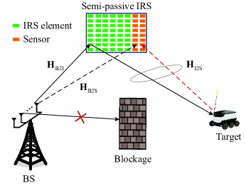
Figure 1: Semi-passive IRS aided localization system.

In this paper, we tackle the above two challenges by applying the semi-passive IRS architecture for localization. To this end, we first derive Cramér-Rao bound (CRB) to characterize a lower bound of the mean squared error (MSE) of the target location and then unveil the relationship between CRB and system parameters. Particularly, the optimal numbers of IRS reflecting elements and sensors to minimize the ToA/DoA estimation error are derived. Then, we propose efficient estimators to estimate the target location. To be specific, the MUSIC algorithm is applied to estimate the target DoA. Then, by transforming the received sensor data into frequency-domain sequences via discrete Fourier transform (DFT), we apply the maximum likelihood (ML) estimator to jointly estimate the ToA and the target-related coefficient. The advantage is that these two steps do not require any iterations, thereby resulting in low computation. Simulation results show that sub-meter level positioning accuracy is achieved even over a long distance from the BS to the target. Moreover, the superiority of semi-passive IRS architecture over the fully-passive IRS is also verified.

II System Model

We consider a localization system consisting of one BS, a semi-passive IRS, and one target with unknown location as shown in Fig. 1. The direct link between the BS and target is blocked due to the surrounding obstacles around the BS. The coordinates of the BS, the semi-passive IRS, and the target are denoted by ${{\bf{q}}_{{\rm{BS}}}}={\left[{{x_{{\rm{BS}}}},{y_{{\rm{BS}}}},{z_{{\rm{BS}}}}}\right]^{T}}$, ${{\bf{q}}_{\rm{I}}}={\left[{{x_{\rm{I}}},{y_{\rm{I}}},{z_{\rm{I}}}}\right]^{T}}$, and ${{\bf{q}}_{\rm{u}}}={\left[{{x_{\rm{u}}},{y_{\rm{u}}},0}\right]^{T}}$, respectively. The semi-passive IRS consists of two parts: reflecting elements and active sensors, where reflecting elements are passive and only used for reconfiguring the phases of incident signals, while the sensors are active and have signal processing abilities. The BS has ${{N_{{\rm{BS}}}}}$ antennas along the $y$ axis and the semi-passive IRS has $N_{\rm r}$ reflecting elements and $N_{\rm s}$ sensors lying on the $y\text{-}o\text{-}z$ plane. We consider a quasi-static flat-fading channel in which the channel state information remains unchanged in the considered frames.

II-A Channel Model

As shown in Fig. 1, the sensors receive signals from two links: BS-IRS (passive side)-target-sensor link and BS-sensor link. Their channel models are described as follows.

The BS-IRS (passive side) channel is modeled as

$${{\bf{H}}_{{\rm{B2I}}}}={\beta_{{\rm{B2I}}}}{{\bf{b}}_{\rm{r}}}\left({\mu_{{\rm{B2I}}}^{\rm{A}}}\right){{\bf{a}}^{H}}\left({\mu_{{\rm{B2I}}}^{\rm{D}}}\right),$$ (1)

where ${\beta_{{\rm{B2I}}}}{\rm{=}}\sqrt{\frac{{{\lambda^{2}}}}{{16{\pi^{2}}d_{{\rm{B2I}}}^{2}}}}$ denotes the large-scale path loss, $\lambda$ represents carrier wavelength, ${d_{{\rm{B2I}}}}$ stands for the distance between the BS and the IRS, ${\mu_{{\rm{B2I}}}^{\rm{D}}}$ and ${\mu_{{\rm{B2I}}}^{\rm{A}}}$ denote the frequency azimuth angle-of-departure (AoD) from the BS to the IRS and the frequency azimuth angle-of-arrival (AoA) at the IRS, respectively, and ${\bf{a}}\left({\mu_{{\rm{B2I}}}^{\rm{D}}}\right)$ and ${{\bf{b}}_{\rm{r}}}\left({\mu_{{\rm{B2I}}}^{\rm{A}}}\right)$ denote the transmit array response vector of the BS and the receive array response vector of IRS given by ${\bf{a}}\left({\mu_{{\rm{B2I}}}^{\rm{D}}}\right){\rm{=}}{\left[{{e^{-\frac{{j\left({{N_{{\rm{BS}}}}-1}\right)\pi\mu_{{\rm{B2I}}}^{\rm{D}}}}{2}}},\ldots,{e^{\frac{{j\left({{N_{{\rm{BS}}}}-1}\right)\pi\mu_{{\rm{B2I}}}^{\rm{D}}}}{2}}}}\right]^{T}}$ and ${{\bf{b}}_{\rm{r}}}\left({\mu_{{\rm{B2I}}}^{\rm{A}}}\right){\rm{=}}{\left[{{e^{-\frac{{j\left({{N_{\rm{r}}}-1}\right)\pi\mu_{{\rm{B2I}}}^{\rm{A}}}}{2}}},\ldots,{e^{\frac{{j\left({{N_{\rm{r}}}-1}\right)\pi\mu_{{\rm{B2I}}}^{\rm{A}}}}{2}}}}\right]^{T}}$, respectively. The channel between the BS and the sensors, i.e., ${{{\bf{H}}_{{\rm{B2S}}}}}$, can be modeled similarly, and thus it is omitted here.

The IRS-target-sensor channel is modeled as

$${{\bf{H}}_{{\rm{I2S}}}}=\alpha{\beta_{{\rm{I2S}}}}{{\bf{b}}_{\rm{s}}}\left({\mu_{{\rm{I2U}}}^{\rm{A}}}\right){\bf{b}}_{\rm{r}}^{T}\left({\mu_{{\rm{I2U}}}^{\rm{D}}}\right),$$ (2)

where ${\beta_{{\rm{I2S}}}}{\rm{=}}\sqrt{\frac{{{\lambda^{2}}{\kappa_{{\rm{RCS}}}}}}{{64{\pi^{3}}d_{{\rm{I2U}}}^{4}}}}$, ${d_{{\rm{I2U}}}}$ denotes the distance between the IRS and the target, ${{\kappa_{{\rm{RCS}}}}}$ represents the radar cross-section, $\alpha\sim{\cal CN}\left({0,1}\right)$ denotes the small fading caused by the fluctuation of the target. In addition, ${{\bf{b}}_{\rm{s}}}\left({\mu_{{\rm{I2U}}}^{\rm{A}}}\right){\rm{=}}{\left[{{e^{-\frac{{j\left({{N_{\rm{s}}}-1}\right)\pi\mu_{{\rm{I2U}}}^{\rm{A}}}}{2}}},\ldots,{e^{\frac{{j\left({{N_{\rm{s}}}-1}\right)\pi\mu_{{\rm{I2U}}}^{\rm{A}}}}{2}}}}\right]^{T}}$ and ${{\bf{b}}_{\rm{r}}}\left({\mu_{{\rm{I2U}}}^{\rm{D}}}\right){\rm{=}}{\left[{{e^{-\frac{{j\left({{N_{\rm{r}}}-1}\right)\pi\mu_{{\rm{I2U}}}^{\rm{D}}}}{2}}},\ldots,{e^{\frac{{j\left({{N_{\rm{r}}}-1}\right)\pi\mu_{{\rm{I2U}}}^{\rm{D}}}}{2}}}}\right]^{T}}$. We consider that the target is in the far field of the semi-passive IRS, the AoD from the IRS (passive side) to the target equals the AoA from the target to the sensors. For notational simplicity, we denote $\mu_{{\rm{I2U}}}$ by $\mu_{{\rm{I2U}}}{\rm{=}}\mu_{{\rm{I2U}}}^{\rm{A}}{\rm{=}}\mu_{{\rm{I2U}}}^{\rm{D}}$.

II-B IRS-aided Sensing Protocol

Since the target position is unknown to the BS, the IRS should adjust different beams with different directions to scan the target. Without loss of generality, we assume that there are $N_{\rm f}$ frames and in each frame, the IRS adjusts beam once. Let ${\bf{\Theta}}\left(n\right){\rm{=diag}}\left({{\bm{\theta}}\left(n\right)}\right)$ with ${\bm{\theta}}\left(n\right)={\left[{{e^{j{\theta_{1}}\left(n\right)}},\ldots,{e^{j{\theta_{{N_{\rm{r}}}}}\left(n\right)}}}\right]^{T}}$ denote the IRS phase shift matrix in the $n$th frame.

The signal received by the sensor at time $t$ in the $n$th frame is given by

$${\bf{\tilde{y}}}\left({n,t}\right) ={{\bf{H}}_{{\rm{I2S}}}}{\bf{\Theta}}\left(n\right){{\bf{H}}_{{\rm{B2I}}}}{\bf{w}}s\left(t-\tau_{\rm tot}\right)$$

$$+{{\bf{H}}_{{\rm{B2S}}}}{\bf{w}}s\left({t-{\tau_{{\rm{B2I}}}}}\right)+{\bf{n}}\left(t\right),\forall n,$$ (3)

where $s\left(t\right)$ stands for the transmitted signal, ${\bf{w}}$ represents the BS beamformer, ${\tau_{{\rm{tot}}}}={\tau_{{\rm{B2I}}}}+2{\tau_{{\rm{I2U}}}}$, ${{\tau_{{\rm{B2I}}}}}$ and ${{\tau_{{\rm{I2U}}}}}$ denote ToAs from the BS to the IRS and from the IRS to the target, respectively, and ${\bf{n}}\left(t\right)$ is the circularly symmetric complex Gaussian noise satisfying ${\bf{n}}\left(t\right)\sim{\cal CN}\left({0,{\sigma^{2}}{{\bf{I}}_{{N_{\rm{s}}}}}}\right)$. As the locations of the BS and the semi-passive IRS are known, the channel information ${{\bf{H}}_{{\rm{B2S}}}}{\bf{w}}s\left({t-{\tau_{{\rm{B2I}}}}}\right)$ can be known by the sensor in advance via offline estimation and can be perfectly canceled before performing target location estimation at the sensor side.

Thus, after removing ${{\bf{H}}_{{\rm{B2S}}}}{\bf{w}}s\left({t-{\tau_{{\rm{B2I}}}}}\right)$ and performing algebraic operations in (3), we can transform (3) into

$${\bf{y}}\left({n,t}\right) =\alpha{\beta_{{\rm{B2I}}}}{\beta_{{\rm{I2S}}}}{{\bf{b}}_{\rm{s}}}\left({\mu_{{\rm{I2U}}}}\right){\bf{b}}_{\rm{r}}^{T}\left({\mu_{{\rm{I2U}}}}\right){\bf{\Theta}}\left(n\right){{\bf{b}}_{\rm{r}}}\left({\mu_{{\rm{B2I}}}^{\rm{A}}}\right)$$

$$\times{{\bf{a}}^{H}}\left({\mu_{{\rm{B2I}}}^{\rm{D}}}\right){\bf{w}}s\left({t-{\tau_{{\rm{tot}}}}}\right)+{\bf{n}}\left(t\right),\forall n.$$ (4)

Obviously, to maximize the power received at the sensor, the BS should directly adjust the beam towards the IRS, i.e., the optimal beamformer $\bf w$ is set as

$${\bf{w}}^{\rm opt}=\sqrt{\frac{{{P_{{\rm{BS}}}}}}{{{N_{{\rm{BS}}}}}}}{\bf{a}}\left({\mu_{{\rm{B2I}}}^{\rm{D}}}\right),$$ (5)

where ${{P_{{\rm{BS}}}}}$ denotes the BS transmit power.

Then, substituting (5) into (4) yields

$${\bf{y}}\left({n,t}\right) ={\beta_{{\rm{target}}}}{{\bf{b}}_{\rm{s}}}\left({\mu_{{\rm{I2U}}}}\right){\bf{b}}_{\rm{r}}^{T}\left({\mu_{{\rm{I2U}}}}\right){\bf{\Theta}}\left(n\right){{\bf{b}}_{\rm{r}}}\left({\mu_{{\rm{B2I}}}^{\rm{A}}}\right)$$

$$\times s\left({t-{\tau_{{\rm{tot}}}}}\right)+{\bf{n}}\left(t\right),$$ (6)

where ${\beta_{{\rm{target}}}}=\alpha\sqrt{{P_{{\rm{BS}}}}{N_{{\rm{BS}}}}}{\beta_{{\rm{B2I}}}}{\beta_{{\rm{I2S}}}}$.

II-C Location Estimation Performance Evaluation via CRB

Since the target location estimation error is difficult to quantify in general, we introduce the CRB as the performance metric, which is essentially a lower bound of any unbiased estimator.

We define a vector of unknown parameters ${{\bf{u}}_{{\rm{position}}}}{\rm{=}}{\left[{{x_{\rm{u}}},y_{\rm{u}},\beta_{{\rm{target}}}^{{\mathop{\rm Re}\nolimits}},\beta_{{\rm{target}}}^{{\mathop{\rm Im}\nolimits}}}\right]^{T}}$, where ${\beta_{{\rm{target}}}^{{\mathop{\rm Re}\nolimits}}}$ and ${\beta_{{\rm{target}}}^{{\mathop{\rm Im}\nolimits}}}$ denote the real and imaginary parts of ${\beta_{{\rm{target}}}}$, respectively. However, it is difficult to derive the Fisher information matrix (FIM) of ${{\bf{u}}_{{\rm{position}}}}$ (denoted by ${{\bf{F}}_{{\rm{position}}}}$), instead we first compute the FIM of vector ${{\bf{u}}_{{\rm{channel}}}}{\rm{=}}{\left[{{\tau_{{\rm{tot}}}},\mu_{{\rm{I2U}}},\beta_{{\rm{target}}}^{{\mathop{\rm Re}\nolimits}},\beta_{{\rm{target}}}^{{\mathop{\rm Im}\nolimits}}}\right]^{T}}$ (denoted by ${{\bf{F}}_{{\rm{channel}}}}$), and then use the chain rule to derive the FIM of ${{\bf{u}}_{{\rm{position}}}}$ as follows:

$${{\bf{F}}_{{\rm{position}}}}=\frac{{\partial{{\bf{u}}_{{\rm{channel}}}}}}{{\partial{{\bf{u}}_{{\rm{position}}}}}}{{\bf{F}}_{{\rm{channel}}}}{\left({\frac{{\partial{{\bf{u}}_{{\rm{channel}}}}}}{{\partial{{\bf{u}}_{{\rm{position}}}}}}}\right)^{T}},$$ (7)

where $\frac{{\partial{{\bf{u}}_{{\rm{channel}}}}}}{{\partial{{\bf{u}}_{{\rm{position}}}}}}{\rm{=}}\left[{\frac{{\partial{\tau_{{\rm{tot}}}}}}{{\partial{{\bf{u}}_{{\rm{position}}}}}}\frac{{\partial\mu_{{\rm{I2U}}}}}{{\partial{{\bf{u}}_{{\rm{position}}}}}}\frac{{\partial\beta_{{\rm{target}}}^{{\mathop{\rm Re}\nolimits}}}}{{\partial{{\bf{u}}_{{\rm{position}}}}}},\frac{{\partial\beta_{{\rm{target}}}^{{\mathop{\rm Im}\nolimits}}}}{{\partial{{\bf{u}}_{{\rm{position}}}}}}}\right]$. Since there are $N_{\rm f}$ frames for localization, we rewrite ${{\bf{F}}_{{\rm{channel}}}}$ into a sum of $N_{\rm f}$ independent FIMs as ${{\bf{F}}_{{\rm{channel}}}}=\sum\limits_{n=1}^{{N_{\rm{f}}}}{{{\bf{F}}_{{\rm{channel}}}}\left(n\right)}$. In the following, we show how to calculate ${{{\bf{F}}_{{\rm{channel}}}}\left(n\right)},\forall n$.

The probability density function of the received signal ${\bf{y}}\left({n,t}\right)$ in (6) conditioned on ${{{\bf{u}}_{{\rm{channel}}}}}$ is given by [12]

$$p\left({{\bf{y}}\left({n,t}\right)}\right)={\eta}\exp\left({-\frac{1}{{{n_{0}}}}\int{{{\left\|{{\bf{y}}\left({n,t}\right)-{\bf{\bar{y}}}\left({n,t}\right)}\right\|}^{2}}{\rm{d}}t}}\right),$$ (8)

where ${n}_{0}$ denotes the noise power density, $\eta$ is a constant which has no contributions on ${{\bf{u}}_{{\rm{position}}}}$, and ${\bf{\bar{y}}}\left({n,t}\right)={\beta_{{\rm{target}}}}{{\bf{b}}_{\rm{s}}}\left({\mu_{{\rm{I2U}}}}\right){\bf{b}}_{\rm{r}}^{T}\left({\mu_{{\rm{I2U}}}}\right){\bf{\Theta}}\left(n\right){{\bf{b}}_{\rm{r}}}\left({\mu_{{\rm{B2I}}}^{\rm{A}}}\right)s\left({t-{\tau_{{\rm{tot}}}}}\right)$. Thus, FIM ${{\bf{F}}_{{\rm{channel}}}}\left(n\right)$ can be computed as

$${{\bf{F}}_{{\rm{channel}}}}\left(n\right)=\left[{\begin{array}[]{*{20}{c}}{{F_{\tau\tau}}\left(n\right)}&{{F_{\tau\mu}}\left(n\right)}&{{{\bf{F}}_{\tau{\bm{\beta}}}}\left(n\right)}\\ {F_{\tau\mu}^{T}\left(n\right)}&{{F_{\mu\mu}}\left(n\right)}&{{{\bf{F}}_{\mu{\bm{\beta}}}}\left(n\right)}\\ {F_{\tau{\bm{\beta}}}^{T}\left(n\right)}&{F_{\mu{\bm{\beta}}}^{T}\left(n\right)}&{{{\bf{F}}_{{\bm{\beta\beta}}}}\left(n\right)}\end{array}}\right],$$ (12)

where ${\bm{\beta}}={\left[{\beta_{{\rm{target}}}^{{\rm{Re}}},\beta_{{\rm{target}}}^{{\rm{Im}}}}\right]^{T}}$. The $(i,j)$ entry of ${{\bf{F}}_{{\rm{channel}}}}\left(n\right)$ is calculated by ${{\bf{F}}_{{\rm{channel}}}}{\left(n\right)_{i,j}}=-{\mathbb{E}}\left\{{\frac{{{\partial^{2}}\ln p\left({{\bf{y}}\left({n,t}\right);{{\bf{u}}_{{\rm{channel}}}}}\right)}}{{\partial{{\bf{u}}_{{\rm{channel,}}i}}\partial{{\bf{u}}_{{\rm{channel,}}j}}}}}\right\}$. The following notation is defined for later use: $\dot{s}\left({t-{\tau_{{\rm{tot}}}}}\right){\rm{=}}\frac{{\partial s\left({t-{\tau_{{\rm{tot}}}}}\right)}}{{\partial\tau}}$, $\ddot{s}\left({t-{\tau_{{\rm{tot}}}}}\right){\rm{=}}\frac{{{\partial^{2}}s\left({t-{\tau_{{\rm{tot}}}}}\right)}}{{{\partial^{2}}\tau}}$, ${{\bf{\dot{b}}}_{\rm{s}}}\left({\mu_{{\rm{I2U}}}}\right)=\frac{{\partial{{\bf{b}}_{\rm{s}}}\left({\mu_{{\rm{I2U}}}}\right)}}{{\mu_{{\rm{I2U}}}}}$, ${{\bf{\ddot{b}}}_{\rm{s}}}\left({\mu_{{\rm{I2U}}}}\right)=\frac{{{\partial^{2}}{{\bf{b}}_{\rm{s}}}\left({\mu_{{\rm{I2U}}}}\right)}}{{{\partial^{2}}\mu_{{\rm{I2U}}}}}$, ${\bf{\dot{b}}}_{\rm{r}}\left({\mu_{{\rm{I2U}}}}\right)=\frac{{\partial{{\bf{b}}_{\rm{r}}}\left({\mu_{{\rm{I2U}}}}\right)}}{{\mu_{{\rm{I2U}}}}}$, ${E_{\rm{s}}}=\int{{{\left|{s\left({n,t-{\tau_{{\rm{tot}}}}}\right)}\right|}^{2}}{\rm{d}}t}$, and ${{\bar{W}}^{2}}=\int{{{\left|{\frac{{\partial s\left({n,t-{\tau_{{\rm{tot}}}}}\right)}}{{\partial\tau}}}\right|}^{2}}{\rm{d}}t/{E_{\rm{s}}}}$. Note that we have the following identities: ${\bf{b}}_{\rm{s}}^{H}\left({\mu_{{\rm{I2U}}}}\right){{\bf{\ddot{b}}}_{\rm{s}}}\left({\mu_{{\rm{I2U}}}}\right)=-\frac{{{\pi^{2}}{N_{\rm{s}}}\left({{N_{\rm{s}}}-1}\right)\left({{N_{\rm{s}}}+1}\right)}}{{12}}$, ${\bf{b}}_{\rm{r}}^{H}\left({\mu_{{\rm{I2U}}}}\right){{{\bf{\dot{b}}}}_{\rm{r}}}\left({\mu_{{\rm{I2U}}}}\right)=0$, and ${\bf{b}}_{\rm{s}}^{H}\left({\mu_{{\rm{I2U}}}}\right){{{\bf{\dot{b}}}}_{\rm{s}}}\left({\mu_{{\rm{I2U}}}}\right)=0$. Then, we can calculate ${{F_{\tau\tau}}\left(n\right)}$, ${{F_{\tau\mu}}\left(n\right)}$, ${{{\bf{F}}_{\tau\bm{\beta}}}\left(n\right)}$, ${{F_{\mu\mu}}\left(n\right)}$, ${{{\bf{F}}_{\mu\bm{\beta}}}\left(n\right)}$, and ${{{\bf{F}}_{\bm{\beta}\bm{\beta}}}\left(n\right)}$ in (12) respectively as

$${{{F}}_{\tau\tau}}\left(n\right){\rm{=}}\frac{{{\rm{2}}{{\left|{{\beta_{{\rm{target}}}}}\right|}^{2}}{N_{\rm{s}}}}}{{{n_{0}}}}{\left|{{\bf{b}}_{\rm{r}}^{T}\left({\mu_{{\rm{I2U}}}}\right){\bf{\Theta}}\left(n\right){{\bf{b}}_{\rm{r}}}\left({\mu_{{\rm{B2I}}}^{\rm{A}}}\right)}\right|^{2}}{{\bar{W}}^{2}}{E_{\rm{s}}},$$ (13)

$${{{F}}_{\tau\mu}}\left(n\right){\rm{=}}\frac{{{\rm{2}}{{\left|{{\beta_{{\rm{target}}}}}\right|}^{2}}{N_{\rm{s}}}}}{{{n_{0}}}}\int{{\mathop{\rm Re}\nolimits}\left\{{{\bf{\dot{b}}}_{\rm{r}}^{T}\left({\mu_{{\rm{I2U}}}}\right){\bf{\Theta}}\left(n\right){{\bf{b}}_{\rm{r}}}\left({\mu_{{\rm{B2I}}}^{\rm{A}}}\right)}\right.}\times$$

$$\left.{{\bf{b}}_{\rm{r}}^{H}\left({\mu_{{\rm{B2I}}}^{\rm{A}}}\right){{\bf{\Theta}}^{H}}\left(n\right){\bf{b}}_{\rm{r}}^{\rm{*}}\left({\mu_{{\rm{I2U}}}}\right)s\left({t-{\tau_{{\rm{tot}}}}}\right){{\dot{s}}^{\rm{*}}}\left({t-{\tau_{{\rm{tot}}}}}\right)}\right\}{\rm{d}}t,$$ (14)

$${{{F}}_{\tau\beta_{{\rm{target}}}^{{\mathop{\rm Re}\nolimits}}}}\left(n\right){\rm{=}}\frac{{{\rm{2}}{N_{\rm{s}}}{{\left|{{\bf{b}}_{\rm{r}}^{T}\left({\mu_{{\rm{I2U}}}}\right){\bf{\Theta}}\left(n\right){{\bf{b}}_{\rm{r}}}\left({\mu_{{\rm{B2I}}}^{\rm{A}}}\right)}\right|}^{2}}}}{{{n_{0}}}}$$

$$\quad\times{\mathop{\rm Re}\nolimits}\left\{{\beta_{{\rm{target}}}\int{\dot{s}\left({n,t-{\tau_{{\rm{tot}}}}}\right){s^{\rm{*}}}\left({n,t-{\tau_{{\rm{tot}}}}}\right){\rm{d}}t}}\right\},$$ (15)

$${{{F}}_{\tau\beta_{{\rm{target}}}^{{\mathop{\rm Im}\nolimits}}}}\left(n\right)=\frac{{{\rm{-2}}{N_{\rm{s}}}{{\left|{{\bf{b}}_{\rm{r}}^{T}\left({\mu_{{\rm{I2U}}}}\right){\bf{\Theta}}\left(n\right){{\bf{b}}_{\rm{r}}}\left({\mu_{{\rm{B2I}}}^{\rm{A}}}\right)}\right|}^{2}}}}{{{n_{0}}}}$$

$$\quad\times{\mathop{\rm Re}\nolimits}\left\{{j\beta_{{\rm{target}}}\int{\dot{s}\left({n,t-{\tau_{{\rm{tot}}}}}\right){s^{\rm{*}}}\left({n,t-{\tau_{{\rm{tot}}}}}\right){\rm{d}}t}}\right\},$$ (16)

$${{{F}}_{\mu\mu}}\left(n\right)=\frac{{{E_{\rm{s}}}{{\left|{{\beta_{{\rm{target}}}}}\right|}^{2}}{N_{\rm{s}}}}}{{6{n_{0}}}}\left({{\rm{1}}2{{\left|{{\bf{\dot{b}}}_{\rm{r}}^{T}\left({\mu_{{\rm{I2U}}}}\right){\bf{\Theta}}\left(n\right){{\bf{b}}_{\rm{r}}}\left({\mu_{{\rm{B2I}}}^{\rm{A}}}\right)}\right|}^{2}}}\right.$$

$$+{{\pi^{2}}\left({{N_{\rm{s}}}-1}\right)\left({{N_{\rm{s}}}+1}\right)\left|{{\bf{b}}_{\rm{r}}^{T}\left({\mu_{{\rm{I2U}}}}\right){\bf{\Theta}}\left(n\right){{\bf{b}}_{\rm{r}}}\left({\mu_{{\rm{B2I}}}^{\rm{A}}}\right)}\right|}\Big{)},$$ (17)

$${{{F}}_{\mu\beta_{{\rm{target}}}^{{\mathop{\rm Re}\nolimits}}}}\left(n\right){\rm{=}}\frac{{2{N_{\rm{s}}}{E_{\rm{s}}}}}{{{n_{0}}}}{\rm{Re}}\left\{{\beta_{{\rm{target}}}{\bf{b}}_{\rm{r}}^{H}\left({\mu_{{\rm{B2I}}}^{\rm{A}}}\right){{\bf{\Theta}}^{H}}\left(n\right){\bf{b}}_{\rm{r}}^{\rm{*}}\left({\mu_{{\rm{I2U}}}}\right)}\right.$$

$$\qquad\qquad\quad\times\left.{{\bf{\dot{b}}}_{\rm{r}}^{T}\left({\mu_{{\rm{I2U}}}}\right){\bf{\Theta}}\left(n\right){{\bf{b}}_{\rm{r}}}\left({\mu_{{\rm{B2I}}}^{\rm{A}}}\right)}\right\},$$ (18)

$${{{F}}_{\mu\beta_{{\rm{target}}}^{{\mathop{\rm Im}\nolimits}}}}\left(n\right){\rm{=}}\frac{{2{N_{\rm{s}}}{E_{\rm{s}}}}}{{{n_{0}}}}{\rm{Re}}\left\{{\beta_{{\rm{target}}}^{*}{\bf{b}}_{\rm{r}}^{H}\left({\mu_{{\rm{B2I}}}^{\rm{A}}}\right){{\bf{\Theta}}^{H}}\left(n\right){\bf{b}}_{\rm{r}}^{\rm{*}}\left({\mu_{{\rm{I2U}}}}\right)}\right.$$

$$\qquad\qquad\quad\times\left.{{\bf{\dot{b}}}_{\rm{r}}^{T}\left({\mu_{{\rm{I2U}}}}\right){\bf{\Theta}}\left(n\right){{\bf{b}}_{\rm{r}}}\left({\mu_{{\rm{B2I}}}^{\rm{A}}}\right)}\right\},$$ (19)

$${{{F}}_{\beta_{{\rm{target}}}^{{\mathop{\rm Re}\nolimits}}\beta_{{\rm{target}}}^{{\mathop{\rm Re}\nolimits}}}}\left(n\right){\rm{=}}\frac{{{\rm{2}}{N_{\rm{s}}}{{\left|{{\bf{b}}_{\rm{r}}^{T}\left({\mu_{{\rm{I2U}}}}\right){\bf{\Theta}}\left(t\right){{\bf{b}}_{\rm{r}}}\left({\mu_{{\rm{B2I}}}^{\rm{A}}}\right)}\right|}^{2}}{E_{\rm{s}}}}}{{{n_{0}}}},$$ (20)

$${{{F}}_{\beta_{{\rm{target}}}^{{\mathop{\rm Re}\nolimits}}\beta_{{\rm{target}}}^{{\mathop{\rm Im}\nolimits}}}}\left(n\right)=0,$$ (21)

$${{{F}}_{\beta_{{\rm{target}}}^{{\mathop{\rm Im}\nolimits}}\beta_{{\rm{target}}}^{{\mathop{\rm Im}\nolimits}}}}\left(n\right){\rm{=}}\frac{{{\rm{2}}{N_{\rm{s}}}{{\left|{{\bf{b}}_{\rm{r}}^{T}\left({\mu_{{\rm{I2U}}}}\right){\bf{\Theta}}\left(t\right){{\bf{b}}_{\rm{r}}}\left({\mu_{{\rm{B2I}}}^{\rm{A}}}\right)}\right|}^{2}}{E_{\rm{s}}}}}{{{n_{0}}}}.$$ (22)

As a result, based on (7) and (13)-(22), the CRB of target position ${\left({{x_{\rm u}},{y_{\rm u}}}\right)^{T}}$ is given by

$${\rm{CRB}}\left[{{{\left({{x_{\rm u}},{y_{\rm u}}}\right)}^{T}}}\right]=\sum\nolimits_{i=1}^{2}{{{\left[{{\bf{F}}_{{\rm{position}}}^{{\rm{-}}1}}\right]}_{i,i}}}.$$ (23)

II-D Performance Analysis

The CRB matrix of ${{{\bf{u}}_{{\rm{channel}}}}}$ is the inverse of the sum of ${{\bf{F}}_{{\rm{channel}}}}\left(n\right)$ in (12) given by

$${\rm{CRB}}\left[{{{\bf{u}}_{{\rm{channel}}}}}\right]{\rm{=}}{\left({\sum\nolimits_{n=1}^{{N_{\rm{f}}}}{{{\bf{F}}_{{\rm{channel}}}}\left(n\right)}}\right)^{-1}}.$$ (24)

For the special case where the IRS phase shift matrix is set as ${{\bf{\Theta}}^{{\rm{opt}}}}\left(n\right)=\mathop{\arg\max}\limits_{{\bf{\Theta}}\left(n\right)}\left|{{\bf{b}}_{\rm{r}}^{T}\left({\mu_{{\rm{I2U}}}}\right){\bf{\Theta}}\left(n\right){{\bf{b}}_{\rm{r}}}\left({\mu_{{\rm{B2I}}}^{\rm{A}}}\right)}\right|$ to maximize the received signal power at the sensors, we have the following proposition.

Proposition 1: With IRS phase shift matrix ${{\bf{\Theta}}^{{\rm{opt}}}}\left(n\right)$ and $\int{\dot{s}\left({t-{\tau_{{\rm{tot}}}}}\right){s^{\rm{*}}}\left({t-{\tau_{{\rm{tot}}}}}\right){\rm{d}}t}{\rm{=}}0$, we can obtain the closed-form CRBs of $\tau_{\rm tot}$ and $\mu_{\rm I2U}$ as

$${\rm{CRB}}\left({{\tau_{{\rm{tot}}}}}\right)=\frac{{{n_{0}}}}{{{\rm{2}}{{\left|{{\beta_{{\rm{target}}}}}\right|}^{2}}{N_{\rm{s}}}N_{\rm{r}}^{2}{N_{\rm{f}}}{{\bar{W}}^{2}}{E_{\rm{s}}}}},$$ (25)

$${\rm{CRB}}\left({{\mu_{{\rm{I2U}}}}}\right)=\frac{{6{n_{0}}}}{{{\pi^{2}}{N_{\rm{s}}}\left({{N_{\rm{s}}}-1}\right)\left({{N_{\rm{s}}}+1}\right)N_{\rm{r}}^{2}{N_{\rm{f}}}{{\left|{{\beta_{{\rm{target}}}}}\right|}^{2}}{E_{\rm{s}}}}}.$$ (26)

Proof: The solution of $\mathop{\arg\max}\limits_{{\bf{\Theta}}\left(n\right)}\left|{{\bf{b}}_{\rm{r}}^{T}\left({\mu_{{\rm{I2U}}}}\right){\bf{\Theta}}\left(n\right){{\bf{b}}_{\rm{r}}}\left({\mu_{{\rm{B2I}}}^{\rm{A}}}\right)}\right|$ is given by ${{\bm{\theta}}^{{\rm{opt}}}}\left(n\right){\rm{=}}\frac{{{{\left({{\rm{diag}}\left({{\bf{b}}_{\rm{r}}^{T}\left({\mu_{{\rm{I2U}}}}\right)}\right){{\bf{b}}_{\rm{r}}}\left({\mu_{{\rm{B2I}}}^{\rm{A}}}\right)}\right)}^{*}}}}{{\left|{{\rm{diag}}\left({{\bf{b}}_{\rm{r}}^{T}\left({\mu_{{\rm{I2U}}}}\right)}\right){{\bf{b}}_{\rm{r}}}\left({\mu_{{\rm{B2I}}}^{\rm{A}}}\right)}\right|}}$. Then, we have ${\left|{{\bf{b}}_{\rm{r}}^{T}\left({\mu_{{\rm{I2U}}}}\right){{\bf{\Theta}}^{{\rm{opt}}}}\left(n\right){{\bf{b}}_{\rm{r}}}\left({\mu_{{\rm{B2I}}}^{\rm{A}}}\right)}\right|^{2}}=N_{\rm{r}}^{2}$ and ${\bf{\dot{b}}}_{\rm{r}}^{T}\left({\mu_{{\rm{I2U}}}}\right){{\bf{\Theta}}^{{\rm{opt}}}}\left(n\right){{\bf{b}}_{\rm{r}}}\left({\mu_{{\rm{B2I}}}^{\rm{A}}}\right)=0$. Together with $\int{\dot{s}\left({t-{\tau_{{\rm{tot}}}}}\right){s^{\rm{*}}}\left({t-{\tau_{{\rm{tot}}}}}\right){\rm{d}}t}{\rm{=}}0$, we have ${{{F}}_{\tau\mu}}\left(n\right)=0$, ${{{F}}_{\tau\beta_{{\rm{target}}}^{{\mathop{\rm Re}\nolimits}}}}\left(n\right)=0$, ${{{F}}_{\tau\beta_{{\rm{target}}}^{{\mathop{\rm Im}\nolimits}}}}\left(n\right)=0$, ${{{F}}_{\mu\beta_{{\rm{target}}}^{{\mathop{\rm Re}\nolimits}}}}\left(n\right)=0$, and ${{{F}}_{\mu\beta_{{\rm{target}}}^{{\mathop{\rm Im}\nolimits}}}}\left(n\right)=0$. As a result, (24) reduces to a diagonal matrix, thus leading to the desired result.

Observing from (25), we can see that the CRB of ${{\tau_{{\rm{tot}}}}}$ is inversely proportional to ${N_{\rm{s}}}N_{\rm{r}}^{2}$. This result can be explained as follows. Since the ToA estimation error is only related to the power received at the sensors regardless of the direction of the signal impinging on the sensors. Moreover, it can be seen from (6) that the received power comes from two aspects. The first aspect is the linear receive beamforming gain of ${\cal O}\left({{N_{\rm{s}}}}\right)$ brought by sensors and the other is the passive beamforming gain of ${\cal O}\left({{N_{\rm{r}}^{2}}}\right)$ brought by the IRS. Different from ToA estimation, the CRB of ${{\mu_{{\rm{I2U}}}}}$ in (25) shows that the DoA estimation error is inversely proportional to ${N_{\rm{s}}}\left({{N_{\rm{s}}}-1}\right)\left({{N_{\rm{s}}}+1}\right)N_{\rm{r}}^{2}$ since it is related to both the received power and the direction of the signal arriving at the sensors. More specifically, the IRS provides the passive beamforming gain of ${\cal O}\left({{N_{\rm{r}}^{2}}}\right)$, while the the sensors not only provide the linear receive beamforming gain but also the spatial direction gain of ${\cal O}\left({N_{\rm{s}}^{3}}\right)$ as in the conventional radar systems [2].

In some applications, we may be interested in either ToA or DoA. The optimal system parameter configuration for each objective can be obtained. Specifically, provided that the total number of active sensors and reflecting elements is fixed (denoted by $N$), i.e., ${N_{\rm{s}}}+{N_{\rm{r}}}={N}$, the optimal ${N_{\rm{r}}}$ to minimize ${\rm{CRB}}\left({{\tau_{{\rm{tot}}}}}\right)$ is given by ${2/3N}$. In addition, the optimal ${N_{\rm{r}}}$ to minimize ${\rm{CRB}}\left({{\mu_{{\rm{I2U}}}}}\right)$ is given by $N_{\rm{r}}^{{\rm{opt}}}=\sqrt[3]{{\left({{N^{3}}-5N}\right)/125+\sqrt{{N^{4}}-2{N^{2}}-5}/25}}+\sqrt[3]{{\left({{N^{3}}-5N}\right)/125-\sqrt{{N^{4}}-2{N^{2}}-5}/25}}$. With optimal ${N_{\rm{r}}^{\rm opt}}$, the optimal ${N_{\rm{s}}}$ is given by $N-N_{\rm{r}}^{{\rm{opt}}}$.

III Target Location Estimation Algorithm Design

In this section, we propose a low-complexity algorithm for estimating DoA ${{\mu_{{\rm{I2U}}}}}$, ToA ${{\tau_{{\rm{tot}}}}}$, and parameter ${\beta_{{\rm{target}}}}$.

III-A Estimate of DoA ${{\mu_{{\rm{I2U}}}}}$

We first stack the received signals in (6) as a matrix form given by

$${\bf{Y}}\left(t\right) ={{\bf{b}}_{\rm{s}}}\left({\mu_{{\rm{I2U}}}}\right)\left({{\beta_{{\rm{target}}}}{\bf{b}}_{\rm{r}}^{T}\left({\mu_{{\rm{I2U}}}}\right)\left[{{\bf{\Theta}}\left(1\right),\ldots,{\bf{\Theta}}\left({{N_{\rm{f}}}}\right)}\right]}\right)$$

$$\times{{\bf{b}}_{\rm{r}}}\left({\mu_{{\rm{B2I}}}^{\rm{A}}}\right)s\left({t-{\tau_{{\rm{tot}}}}}\right){\rm{+}}{\bf{N}}\left(t\right).$$ (27)

The auto-correlation matrix of ${{\bf{y}}\left({n,t}\right)}$ is approximately as

$${{\bf{R}}_{{\bf{Y}}\left(t\right)}}{\rm{=}}\frac{1}{{{N_{\rm{f}}}}}{\bf{Y}}\left(t\right){{\bf{Y}}^{H}}\left(t\right).$$ (28)

As there is only one target direction, the largest eigenvalue of ${{\bf{R}}_{{\bf{Y}}\left(t\right)}}$ spans the signal subspace and the remaining $N_{\rm s}-1$ eigenvectors correspond to the noise subspace. Specifically, performing singular value decomposition on ${{\bf{R}}_{{\bf{Y}}\left(t\right)}}$, we have

$${{\bf{R}}_{{\bf{Y}}\left(t\right)}}{\rm{=}}\left[{\begin{array}[]{*{20}{c}}{{{\bf{U}}_{\rm{s}}}}&{{{\bf{U}}_{\rm{n}}}}\end{array}}\right]{\rm{diag}}\left({{\Sigma_{\rm{s}}},{{\bf{\Sigma}}_{\rm{n}}}}\right){\left[{\begin{array}[]{*{20}{c}}{{{\bf{U}}_{\rm{s}}}}&{{{\bf{U}}_{\rm{n}}}}\end{array}}\right]^{H}},$$ (31)

where the eigenvalues of ${{\bf{R}}_{{\bf{Y}}\left(t\right)}}$ are sorted in decreasing order, ${{\bf{U}}_{\rm{s}}}{\kern 1.0pt}\in{{\mathbb{C}}^{{N_{\rm{s}}}\times 1}}$, and ${{\bf{U}}_{\rm{n}}}\in{{\mathbb{C}}^{{N_{\rm{s}}}\times\left({{N_{\rm{s}}}-1}\right)}}$. Following [13], the MUSIC method is applied:

$$\hat{\mu}_{{\rm{I2U}}}{\rm{=}}\mathop{\arg\max}\limits_{{\mu_{{\rm{I2U}}}}}\frac{1}{{{\bf{b}}_{\rm{s}}^{H}\left({\mu_{{\rm{I2U}}}}\right){{\bf{U}}_{\rm{n}}}{\bf{U}}_{\rm{n}}^{H}{\bf{b}}_{\rm{s}}\left({\mu_{{\rm{I2U}}}}\right)}},$$ (32)

where the estimate of ${{\mu_{{\rm{I2U}}}}}$ can be obtained by a simple one-dimensional search ranging from $-1$ to $1$.

III-B Estimate of ToA ${{\tau_{{\rm{tot}}}}}$ and Target Parameter ${\beta_{{\rm{target}}}}$

We collect $N_{\rm f}$ pieces of signals in (6) and sum them, yielding

$${\bf{y}}\left(t\right) ={\beta_{{\rm{target}}}}{{\bf{b}}_{\rm{s}}}\left({\mu_{{\rm{I2U}}}}\right){\bf{b}}_{\rm{r}}^{T}\left({\mu_{{\rm{I2U}}}}\right)\sum\limits_{n=1}^{{N_{\rm{f}}}}{{\bf{\Theta}}\left(n\right)}$$

$$\times{{\bf{b}}_{\rm{r}}}\left({\mu_{{\rm{B2I}}}^{\rm{A}}}\right)s\left({t-{\tau_{{\rm{tot}}}}}\right)+{\bf{\tilde{n}}}\left(t\right),$$ (33)

where ${\bf{\tilde{n}}}\left(t\right)\sim{\cal CN}\left({0,{N_{\rm{f}}}{\sigma^{2}}{{\bf{I}}_{{{\rm{N}}_{\rm{s}}}}}}\right)$. Then, summing all the sensor signals given in (33), i.e.,

$${\bar{y}}\left(t\right) ={\rm{sum}}\left({{\bf{y}}\left(t\right)}\right)={\beta_{{\rm{target}}}}f\left({\mu_{{\rm{I2U}}}}\right){\bf{b}}_{\rm{r}}^{T}\left({\mu_{{\rm{I2U}}}}\right)\sum\limits_{n=1}^{{N_{\rm{f}}}}{{\bf{\Theta}}\left(n\right)}$$

$$\times{{\bf{b}}_{\rm{r}}}\left({\mu_{{\rm{B2I}}}^{\rm{A}}}\right)s\left({t-{\tau_{{\rm{tot}}}}}\right)+n\left(t\right),$$ (34)

where $f\left({\mu_{{\rm{I2U}}}}\right){\rm{=sum}}\left({{{\bf{b}}_{\rm{s}}}\left({\mu_{{\rm{I2U}}}}\right)}\right)$ and $n\left(t\right)\sim{\cal CN}\left({0,{N_{\rm{f}}}{N_{\rm{s}}}{\sigma^{2}}}\right)$. Here, we estimate ${{\tau_{{\rm{tot}}}}}$ and ${\beta_{{\rm{target}}}}$ by using DFT technique. Specifically, denote by $T_{\rm s}$ and ${\hat{N}}_{\rm s}$ the sampling period and the number of sampling points, respectively, and define $Y\left(k\right)$, $S\left(k\right)$, and $N\left(k\right)$, $k=-{{\hat{N}}_{\rm s}\mathord{\left/{\vphantom{N{2,\ldots,}}}\right.\kern-1.2pt}{2,\ldots,}}{{\hat{N}}_{\rm s}\mathord{\left/{\vphantom{N{2+1}}}\right.\kern-1.2pt}{2+1}}$, as the DFTs of $y\left({l{T_{\rm{s}}}}\right)$, $s\left({l{T_{\rm{s}}}}\right)$, and $n\left({l{T_{\rm{s}}}}\right)$, $l=0,\ldots,{{\hat{N}}_{\rm{s}}-1}$, respectively. Then, the following equality holds:

$$Y\left(k\right)={{\bar{\beta}}_{{\rm{target}}}}S\left(k\right){e^{jw_{\rm tot}k}}+N\left(k\right),$$ (35)

where ${w_{{\rm{tot}}}}={{-2\pi{\tau_{{\rm{tot}}}}}\mathord{\left/{\vphantom{{-2\pi{\tau_{{\rm{tot}}}}}{\left({{T_{\rm{s}}}{{\hat{N}}_{\rm{s}}}}\right)}}}\right.\kern-1.2pt}{\left({{T_{\rm{s}}}{{\hat{N}}_{\rm{s}}}}\right)}}$ and ${{\bar{\beta}}_{{\rm{target}}}}={\beta_{{\rm{target}}}}f\left({\mu_{{\rm{I2U}}}}\right){\bf{b}}_{\rm{r}}^{T}\left({\mu_{{\rm{I2U}}}}\right)\sum\limits_{n=1}^{{N_{\rm{f}}}}{{\bf{\Theta}}\left(n\right)}{{\bf{b}}_{\rm{r}}}\left({\mu_{{\rm{B2I}}}^{\rm{A}}}\right)$. The ML estimator for ${w_{{\rm{tot}}}}$ and ${{\bar{\beta}}_{{\rm{target}}}}$ based on (35) is given by

$$\left({{{\hat{w}}_{{\rm{tot}}}},{{\hat{\beta}}_{{\rm{target}}}}}\right)_{\rm ML}=$$

$$\mathop{\arg\min}\limits_{{w_{{\rm{tot}}}},{{\bar{\beta}}_{{\rm{target}}}}}\sum\nolimits_{k={{-N}\mathord{\left/{\vphantom{{-N}2}}\right.\kern-1.2pt}2}}^{{N\mathord{\left/{\vphantom{N2}}\right.\kern-1.2pt}2}+1}{{{\left|{Y\left(k\right)-{{\bar{\beta}}_{{\rm{target}}}}S\left(k\right){e^{j{w_{{\rm{tot}}}}k}}}\right|}^{2}}}.$$ (36)

Taking the first-order derivative of (36) with respect to ${{{\bar{\beta}}_{{\rm{target}}}}}$ and setting it to zero, we have

$${{\hat{\beta}}_{{\rm{target}}}}=\frac{{\sum\nolimits_{k={{-N}\mathord{\left/{\vphantom{{-N}2}}\right.\kern-1.2pt}2}}^{{N\mathord{\left/{\vphantom{N2}}\right.\kern-1.2pt}2}+1}{{S^{*}}\left(k\right)Y\left(k\right){e^{-j{w_{{\rm{tot}}}}k}}}}}{{\sum\nolimits_{k={{-N}\mathord{\left/{\vphantom{{-N}2}}\right.\kern-1.2pt}2}}^{{N\mathord{\left/{\vphantom{N2}}\right.\kern-1.2pt}2}+1}{{{\left|{S\left(k\right)}\right|}^{2}}}}}.$$ (37)

Then, substituting (37) into (36), the ML estimator of ${{\hat{w}}_{{\rm{tot}}}}$ is given by

$${{\hat{w}}_{{\rm{tot}}}}=\mathop{\arg\min}\nolimits_{{w_{{\rm{tot}}}}}{\left|{\sum\nolimits_{k={{-N}\mathord{\left/{\vphantom{{-N}2}}\right.\kern-1.2pt}2}}^{{N\mathord{\left/{\vphantom{N2}}\right.\kern-1.2pt}2}+1}{{S^{*}}\left(k\right)Y\left(k\right){e^{-j{w_{{\rm{tot}}}}k}}}}\right|^{2}},$$ (38)

which can be solved by a one-dimensional search.

Finally, based on the geometric relationship $\hat{\mu}_{{\rm{I2U}}}=\frac{{{y_{\rm{I}}}-{y_{\rm{u}}}}}{{\left\|{{{\bf{q}}_{\rm{u}}}-{{\bf{q}}_{\rm{I}}}}\right\|}}$ and ${{\hat{\tau}}_{{\rm{I2U}}}}{\rm{=}}\frac{{\left\|{{{\bf{q}}_{\rm{u}}}-{{\bf{q}}_{\rm{I}}}}\right\|}}{c}$ and together with (32) and (38), the coordinates of the target can be calculated as

$$\left\{\begin{array}[]{l}{{\hat{x}}_{\rm{u}}}=\sqrt{{c^{2}}\hat{\tau}_{{\rm{I2U}}}^{2}{\rm{-}}{{\left({{y_{\rm{I}}}-{{\hat{y}}_{\rm{u}}}}\right)}^{2}}{\rm{-}}z_{\rm{I}}^{2}}{\rm{+}}{x_{\rm{I}}},\\ {{\hat{y}}_{\rm{u}}}={y_{\rm{I}}}-c\hat{\mu}_{{\rm{I2U}}}{{\hat{\tau}}_{{\rm{I2U}}}}.\end{array}\right.$$ (41)

The total complexity for estimating target location is given by ${\cal O}\left({N_{\rm{s}}^{3}+{T_{1}}N_{\rm{s}}^{2}+N_{\rm{s}}{N_{{\rm{frame}}}}+\hat{N}_{\rm{s}}^{2}+{T_{2}}N}\right)$.

IV Numerical Results

In this section, we perform numerical experiments to evaluate the localization performance assisted by the semi-passive IRS. The BS, IRS, and target are located at $(0,0,0)$ m, $(-10,50,2)$ m, and $(5,60,0)$ m, respectively. We consider the chirp signal $s(t)$ as $s\left(t\right)={e^{j2\pi B\left({t+{\nu}{t^{2}}}\right)}},0\leq t\leq{1\mathord{\left/{\vphantom{1B}}\right.\kern-1.2pt}B}$, where $B$ and $\nu$ represent the signal bandwidth and frequency rate, respectively. Unless otherwise specified, other system parameters are set as follows: $N_{\rm BS}=6$, $N_{\rm s}=6$, $N_{\rm r}=50$, $N_{\rm f}=6$, ${\hat{N}}_{\rm s}=64$, ${{\kappa_{{\rm{RCS}}}}}=7~{}{\rm dBsm}$, $\nu={10^{6}}$, $B=1.5~{}{\rm MHz}$ , $\nu=10^{6}$, ${T_{\rm{s}}}=1/\left({B{{\hat{N}}_{\rm{s}}}}\right)$, ${n}_{0}=-150~{}{\rm dBm}/{\rm Hz}$, and $P_{\rm BS}=40~{}{\rm dBm}$. The estimation performance of direction $\mu_{\rm I2U}$ and location ${\bf q}_{\rm u}$ is evaluated by the root MSE (RMSE) [8].

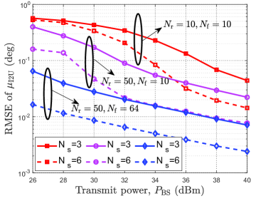
Figure 2: RMSE of $\mu_{\rm I2U}$ versus $P_{\rm BS}$.

In Fig. 2, we evaluate the effectiveness of the proposed semi-passive IRS scheme by plotting the $\mu_{\rm I2U}$-RMSE versus $P_{\rm BS}$ under different $N_{\rm s}$, $N_{\rm r}$, and $N_{\rm f}$. It is observed that a larger number of sensors $N_{\rm s}$, a lower $\mu_{\rm I2U}$-RMSE is achieved since the higher array gain can be provided at the sensors. In addition, one can observe that with a larger number of reflecting elements $N_{\rm r}$, a lower $\mu_{\rm I2U}$-RMSE is achieved. This is because a higher passive beamforming gain can be provided by the IRS. Moreover, the $\mu_{\rm I2U}$-RMSE can be significantly reduced with more time used for adjusting the IRS phase-shift vector, i.e., $N_{\rm f}$. This attributes to two reasons. First, with a higher $N_{\rm f}$, more diversity gain can be achieved since different channels are generated. Second, with a higher $N_{\rm f}$, a fine-grained scanning for a target can be achieved by applying the DFT-based IRS phase shift matrix, which indicates that a higher probability of illuminating the target can be obtained.

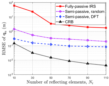
Figure 3: RMSE of ${\bf q}_{\rm u}$ versus $N_{\rm r}$.

To show the superiority of the semi-passive IRS scheme, we compare the following schemes: 1) Semi-passive, DFT: the proposed scheme; 2) Semi-passive, random: the semi-passive IRS architecture is adopted while the IRS phase shifts follow a uniform distribution over $\left[{0,2\pi}\right)$ during each frame; 3) Fully-passive, IRS: there are no sensors at the IRS, and the BS estimates target location via echo signals reflected by the IRS (For a fair comparison, the number of BS receive antennas is set the same as the number of sensors). 4) CRB: the RMSE is derived based on the CRB given in (23). In Fig. 3, we study the impact of $N_{\rm r}$ on the target location estimation under $P_{\rm BS}=34$ dBm. It is observed that our proposed scheme outperforms the fully-passive IRS scheme. The reason is that the signal traveling distance by the proposed scheme is much shorter than that by the fully-passive IRS scheme. In addition, the sensing performance using the DFT-based IRS phase-shift matrix outperforms that using the random-based IRS phase-shift matrix, which shows its superiority. Furthermore, the performance gap between the proposed scheme and the CRB scheme becomes larger when $N_{\rm r}$ increases. This is because that the passive gain brought by the IRS is difficult to fully reap at the sensors since the target direction is unknown.

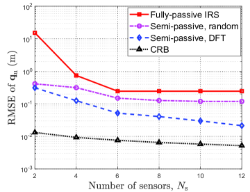
Figure 4: RMSE of ${\bf q}_{\rm u}$ versus $N_{\rm s}$.

In Fig. 4, the impact of $N_{\rm s}$ on the target location estimation is studied. It can be seenthat the proposed scheme outperforms the other benchmark schemes except for the CRB, especially the performance gap becomes more pronounced when $N_{\rm s}$ is large, which again demonstrates the superiority of the proposed scheme. In addition, the ${\bf q}_{\rm u}$-RMSE of the fully-passive IRS scheme nearly remains unchanged while that of the proposed scheme further decreases when $N_{\rm s}\geq 6$. This is because that the spatial direction gain can not be exploited by the fully fully-passive IRS scheme. Furthermore, one can observe that although there is a large performance gap between the proposed scheme and the CRB when $N_{\rm s}\leq 6$, the achieved ${\bf q}_{\rm u}$-RMSE of the proposed scheme approaches the CRB when $N_{\rm s}$ becomes large.

V Conclusion

In this paper, we studied the target localization under the semi-passive IRS architecture. The system parameters including the number of frames, number of IRS reflecting elements, and number of sensors, on the location estimation performance based on the CRB are theoretically analyzed. Then, we further proposed a low-complexity algorithm to estimate the location. More specifically, we first applied the MUSIC method to estimate the target direction, and transformed the time-domain signal sequence into the frequency-domain based on the DFT, then adopted the ML criterion to jointly estimate the time delay and the target-related coefficient. Simulation results demonstrated the superiority of semi-passive IRS architecture over the fully-passive IRS architecture and showed that sub-meter level positioning accuracy can be achieved over a long localization range.

References

• [1] 3GPP, “Study on integrated sensing and communication,” Accessed on July, 1, 2023. [Online]. Available: https://portal.3gpp.org/desktopmodules/Specifications/SpecificationDetails.aspx?specificationId=4044.
• [2] H. C. So, “Source localization: Algorithms and analysis,” Handbook of Position Location: Theory, Practice, and Advances, pp. 25–66, 2011.
• [3] Q. Wu, X. Guan, and R. Zhang, “Intelligent reflecting surface-aided wireless energy and information transmission: An overview,” Proc. IEEE, vol. 110, no. 1, pp. 150–170, Jan. 2022.
• [4] G. Chen, Q. Wu, W. Chen, D. W. K. Ng, and L. Hanzo, “IRS-aided wireless powered MEC systems: TDMA or NOMA for computation offloading?” IEEE Tran. Wireless Commun., vol. 22, no. 2, pp. 1201–1218, Feb. 2023.
• [5] G. Zhou, C. Pan, H. Ren, K. Wang, and A. Nallanathan, “Intelligent reflecting surface aided multigroup multicast MISO communication systems,” IEEE Trans. Signal Process., vol. 68, pp. 3236–3251, Apr. 2020.
• [6] M. Hua, Q. Wu, C. He, S. Ma, and W. Chen, “Joint active and passive beamforming design for IRS-aided radar-communication,” IEEE Trans. Wireless Commun., vol. 22, no. 4, pp. 2278–2294, Apr. 2023.
• [7] K. Meng, Q. Wu, R. Schober, and W. Chen, “Intelligent reflecting surface enabled multi-target sensing,” IEEE Trans. Commun., vol. 70, no. 12, pp. 8313–8330, Dec. 2022.
• [8] X. Shao, C. You, W. Ma, X. Chen, and R. Zhang, “Target sensing with intelligent reflecting surface: Architecture and performance,” IEEE J. Sel. Areas Commun., vol. 40, no. 7, pp. 2070–2084, Jul. 2022.
• [9] K. Keykhosravi, M. F. Keskin, G. Seco-Granados, and H. Wymeersch, “SISO RIS-enabled joint 3D downlink localization and synchronization,” in Proc. ICC, Montreal, QC, Canada, 2021, pp. 1–6.
• [10] A. Elzanaty, A. Guerra, F. Guidi, and M.-S. Alouini, “Reconfigurable intelligent surfaces for localization: Position and orientation error bounds,” IEEE Trans. Signal Process., vol. 69, pp. 5386–5402, Aug. 2021.
• [11] X. Hu, C. Liu, M. Peng, and C. Zhong, “IRS-based integrated location sensing and communication for mmwave SIMO systems,” IEEE Trans. Wireless Commun., vol. 22, no. 6, pp. 4132–4145, Jun. 2023.
• [12] Y. Fu and Z. Tian, “Cramer–rao bounds for hybrid TOA/DOA-based location estimation in sensor networks,” IEEE Signal Process. Lett., vol. 16, no. 8, pp. 655–658, Aug. 2009.
• [13] M. Cheney, “The linear sampling method and the MUSIC algorithm,” Inverse problems, vol. 17, no. 4, p. 591, 2001.