Holographic Complexity with Different Gravitational Observables

Abstract

We investigate a more general conjugate regarding the holographic complexity: complexity equals any gravitational observables [Phys. Rev. Lett. 128, 081602 (2022)], which is an extension of the complexity equals volume proposal. These gravitational observables are referred to as generalized volumes. In this paper, we investigate the generalized volume-complexity for the planar anti-de Sitter black hole and the charged Banados-Teitelboim-Zanelli black hole with different gravitational observables. We note that when anchored at the same boundary time, there may be more than one extremal hypersurface. Determining which one can represent the complexity has become a question that requires further discussion. For the complexity equals volume proposal, the complexity is thought to be proportional to a maximal volume of a hypersurface anchored on the boundary time slice. However, in our research, we find that the size relationship of the gravitational observables on these extremal generalized volume slices are not fixed, but change over time. We refer to this moment of the change as the turning time.

1 Introduction

In the last three decades, the holographic principle has attracted widespread attention Belin:2021bga ; Belin:2022xmt ; Jorstad:2023kmq ; Wang:2023eep ; Omidi:2022whq ; Baggioli:2021xuv ; He:2021xoo ; Akhavan:2019zax ; Omidi:2020oit ; Carmi:2016wjl ; OuYang:2020mpa ; Maldacena:1997re ; Maldacena:2003nj ; Maldacena:2013xja ; Susskind:2016jjb ; Couch:2016exn ; Qu:2022zwq ; Qu:2021ius ; Shenker:2013pqa ; Yang:2019gce ; An:2022lvo ; Stanford:2014jda ; Roberts:2014isa ; Susskind:2014rva ; Susskind:2014moa ; Brown:2015bva ; Brown:2015lvg ; Carmi:2017jqz ; Chapman:2018dem ; Chapman:2018lsv ; Swingle:2017zcd ; Fu:2018kcp ; Cai:2016xho ; Yang:2017hbf ; Guo:2017rul ; Couch:2018phr ; Zhang:2022quy ; Susskind:2014jwa ; Chapman:2016hwi ; Cai:2017sjv ; An:2018xhv ; Goto:2018iay ; Bernamonti:2019zyy ; Bernamonti:2021jyu ; Hartnoll:2008vx ; Hartnoll:2020fhc ; Shi:2021rnd . In 1997, Maldacena made the first concrete realization of the holographic principle Maldacena:1997re . The calculation shows that the conformal field theory (CFT) of $d$-dimensional space-time is equivalent to the quantum gravity theory in $(d+1)$-dimensional asymptotic anti-de Sitter (AdS) space-time, known as the AdS/CFT correspondence Maldacena:1997re ; Maldacena:2003nj . After 26 years of development, the AdS/CFT correspondence has become a popular and important research direction in quantum gravity and quantum information.

On the other hand, Susskind and Maldacena proposed a new idea regarding the holographic principle Maldacena:2013xja . They observed the similarities between the Einstein-Podolsky-Rosen (EPR) paradox and the Einstein-Rosen (ER) bridge and referred to this as the ER = EPR relation Maldacena:2013xja ; Susskind:2016jjb . According to ER = EPR, two systems are connected by an ER bridge if and only if they are entangled. The ER bridge is not a static object, it grows linearly with time for a very long time. However, for a black hole system, the dual system reaches thermal equilibrium quickly. Therefore, entanglement entropy is not enough. For a complete description of the growth of the ER bridge, Susskind introduced quantum computational complexity as a measure of the volume growth of the ER bridge Susskind:2014rva .

Complexity quantifies the level of difficulty associated with performing a task using a set of simple operations. In quantum complexity, a quantum circuit is constructed by combining simple gates that act on a few qubits to perform a particular operation using a unitary operator. In the context of black holes and holography, quantum complexity has recently triggered significant interest, offering a new perspective in the ongoing effort to connect quantum information theory with quantum gravity. Within the framework of AdS/CFT, there are three important proposals regarding the holographic complexity: complexity equals volume (CV) Stanford:2014jda ; Susskind:2014rva ; Susskind:2014moa , complexity equals action (CA) Brown:2015bva ; Brown:2015lvg , and complexity equals spacetime volume (CV 2.0) Couch:2016exn .

The CV proposal maintains that complexity is determined by the maximal volume slice of a hypersurface anchored on the CFT boundary, i.e.

$$\mathcal{C}_{V}=\max_{\partial\Sigma}\left[\frac{V(\Sigma)}{G_{N}L}\right],$$ (1)

where $\Sigma$ is a hypersurface anchored on the boundary CFT slice, $G_{N}$ denotes Newton’s constant in the bulk gravitational theory, and $L$ is a constant with length dimension which often replaced by AdS radius. Based on the CV proposal, Stanford and Susskind calculated the maximum volume hypersurface inside the AdS black hole after it is disturbed by shock wave geometries and proposed the butterfly effect of complexity Stanford:2014jda . Recently, an analytical expression about the butterfly effect of complexity for an inverted harmonic oscillator was obtained in Refs. Qu:2022zwq ; Qu:2021ius .

For the CA proposal, complexity is defined as the action of the Wheeler-de Witt patch, which is given by

$$\mathcal{C}_{A}=\frac{I_{\mathrm{{WdW}}}}{\pi\hbar},$$ (2)

where the Wheeler-de Witt patch is the set of all spacelike hypersurfaces in spacetime Carmi:2016wjl . And the CV 2.0 proposal is optimized based on the first two conjectures. In this case, complexity equals the volume of the Wheeler-de Witt patch, that is

$$\mathcal{C}_{SV}=\frac{V_{\mathrm{{WdW}}}}{G_{N}L^{2}}.$$ (3)

In recent years, there is dramatic progress toward holographic complexity Carmi:2016wjl ; Carmi:2017jqz ; Chapman:2018dem ; Chapman:2018lsv ; Akhavan:2019zax ; Omidi:2020oit ; Swingle:2017zcd ; Fu:2018kcp ; Cai:2016xho ; Yang:2017hbf ; Guo:2017rul ; Couch:2018phr ; Zhang:2022quy ; Susskind:2014jwa ; Chapman:2016hwi ; Cai:2017sjv ; An:2018xhv ; Goto:2018iay ; Bernamonti:2019zyy ; Bernamonti:2021jyu ; Belin:2022xmt ; Belin:2021bga ; Jorstad:2023kmq ; Wang:2023eep ; Omidi:2022whq , complexity of holographic superconductor Yang:2019gce ; Shi:2021rnd ; An:2022lvo , circuit complexity in quantum field theory Jefferson:2017sdb ; Hackl:2018ptj ; Guo:2018kzl ; Caceres:2019pgf ; Ruan:2020vze ; Roca-Jerat:2023mjs , Krylov complexity Parker:2018yvk ; Caputa:2021sib ; Dymarsky:2021bjq ; Avdoshkin:2022xuw ; Bhattacharjee:2022vlt ; Trigueros:2021rwj ; Camargo:2022rnt ; Camargo:2023eev or complexity in de Sitter space Reynolds:2017lwq ; Jorstad:2022mls . Among them, all of holographic complexity proposals have ambiguous definitions, just like the ill-defined constant $L$ in the CV or CV 2.0 proposal, or a similarly indeterminate length scale that occurs on the null boundaries of the Wheeler-de Witt patch. In this regard, some scholars believe that this ambiguity is not a shortcoming of the theory itself, but a feature of holographic complexity. Because there are similar ambiguities in quantum computational complexity, such as the choice of a quantum gate set. The concept of holographic complexity was generalized in Ref. Belin:2021bga ; Belin:2022xmt ; Jorstad:2023kmq . The authors defined the new gravitational observable as the generalized volume-complexity, i.e.

$$\mathcal{O}_{F_{1},\Sigma_{F_{2}}}(\Sigma_{\mathrm{{CFT}}})=\frac{1}{G_{N}L}\int_{\Sigma_{F_{2}}}d^{d}\sigma\sqrt{h}~{}F_{1}(g_{\mu\nu};X^{\mu}),$$ (4)

where $\Sigma_{F_{2}}$ is an codimension-one hypersurface anchored on the CFT slice $\Sigma_{\mathrm{{CFT}}}$, $h$ is the induced metric on the $\Sigma_{F_{2}}$, both $F_{1}$ and $F_{2}$ are scalar functions of the bulk metric $g_{\mu\nu}$ and of an embedding coordinate $X^{\mu}$ of the $\Sigma_{F_{2}}$. If the CFT slice is a constant time slice in the boundary CFT, $\Sigma_{\mathrm{{CFT}}}$ can be rewritten as $\Sigma_{\tau}$, i.e., $\partial\Sigma_{F_{2}}=\Sigma_{\tau}$. $\Sigma_{F_{2}}$ is determined by

$$\delta_{X}\left(\int_{\Sigma_{F_{2}}}d^{d}\sigma\sqrt{h}~{}F_{2}(g_{\mu\nu};X^{\mu})\right)=0.$$ (5)

In general case, there is no correlation between $F_{1}$ and $F_{2}$. However, for $F_{1}=F_{2}=1$, the extremal hypersurface obtained by Eq. (5) is the extremal volume slice in the CV proposal (1). Extending this example, they analyzed in detail the case where $F_{1}=F_{2}=a(r)$, and the conjecture that “complexity equals anything” is validated across multiple models Omidi:2022whq .

In our previous work Wang:2023eep , we considered the generalized volume-complexity for the four-dimensional RN-AdS black hole, whose growth rates exhibit a discontinues change at a certain boundary time. We referred to this boundary time as the turning time. In this paper, we investigate the generalized volume-complexity for the planar AdS black hole and the charged BTZ black hole with some different gravitational observables. We find that the turning time also exists.

In Sec. 2, we review the generalized volume-complexity for the planar AdS black hole and obtain the functional expressions of the complexity and the complexity growth rate. In Sec. 3, we extend the example provided in Ref. Belin:2021bga . Specifically, we choose the concrete expression of the scalar function $F_{1}=F_{2}=a(r)$ as $a(r)=1+\sum_{j=1}^{N}(-1)^{j}\lambda_{j}(L^{4}C^{2})^{j}$ with $C^{2}\equiv C_{\mu\nu\sigma\rho}C^{\mu\nu\sigma\rho}$ the square of the Weyl tensor and $\lambda_{j}$ the coupling constants. We explicitly analyze the cases of $N=2$ and $N=3$. In this situation, we note that there may be more than one extremal hypersurface when anchor at the same boundary time. By calculating the generalized volume, we also observe the discontinues change at a certain boundary time, i.e., turning time. In Sec. 4, we consider the generalized volume-complexity for the charged BTZ black hole. Since the Weyl tensor is always zero in $(2+1)$-dimensional space-time, we select $1-\lambda L^{2}F_{\mu\nu}F^{\mu\nu}$ to construct the scalar function $a(r)$. As in the previous sections, we still analyze the relation between the turning time of the charged BTZ black hole and the coupling constant $\lambda$. Our findings lead to a conclusion similar to that of Sec. 3. Lastly, we present the discussion and conclusion in Sec. 5.

2 Holographic Complexity for Planar AdS Black Holes

We follow the model used in Ref. Belin:2021bga . The metric of the $(d+1)$-dimensional eternal AdS planar black hole can be described in Eddington-Finkelstein coordinates:

$$ds^{2}=-f(r)dv^{2}+2dvdr+\frac{r^{2}}{L^{2}}d\vec{x}^{2},$$ (6)

where $f(r)=\frac{r^{2}}{L^{2}}\left(1-\frac{r_{h}^{d}}{r^{d}}\right)$ and $v=t+r_{*}(r)$ with $r_{*}(r)=-\int_{r}^{\infty}\frac{dr^{\prime}}{f(r^{\prime})}$. This geometry is regarded as the dual of two decoupled CFTs on planar spatial slices $\Sigma$, which are entangled in the thermofield double (TFD) state

$$\left|\psi_{\mathrm{TFD}}(\tau)\right\rangle=\sum_{{n}}e^{-\beta E_{n}/2-iE_{n}\tau}|n\rangle_{\mathrm{L}}\otimes|n\rangle_{\mathrm{R}},$$ (7)

where $\beta$ is the inverse of the temperature, $E_{n}$ is the energy, $L$ and $R$ symbolize the two entangled sides of the planar AdS black hole and label the quantum states $|n\rangle_{L}$ and $|n\rangle_{R}$, respectively. The time $\tau$ is associated with the left and right boundaries with $t_{L}=t_{R}={\tau}/2$. According to Ref. Belin:2021bga , the general expression of complexity can be obtained by

$$\mathcal{C}=\max_{\partial\Sigma=\Sigma_{\tau}}\left[\frac{1}{G_{\mathrm{N}}L}\int_{\Sigma}d^{d}\sigma\sqrt{h}~{}a(r)\right],$$ (8)

where $\sigma$ is a radial coordinate on the hypersurface $\Sigma$. Thanks to the planar symmetric, we can rewrite Eq. (8) as

$$\mathcal{C}=\frac{V_{d-1}}{G_{N}L}\int_{\Sigma}d\sigma\left(\frac{r}{L}\right)^{d-1}\sqrt{-f(r)\dot{v}^{2}+2\dot{v}\dot{r}}~{}a(r)\equiv\frac{V_{d-1}}{G_{N}L}\int_{\Sigma}d\sigma\mathcal{L}(r,\dot{v},\dot{r}),$$ (9)

where $V_{d-1}$ denotes the volume element of the spatial directions ${\vec{x}}$. We can refer to $\mathcal{C}$ as the generalized volume-complexity, and treat the integrand as the Lagrangian $\mathcal{L}$. First of all, we parameterize Eq. (9) and fix the gauge by choosing

$$\sqrt{-f(r)\dot{v}^{2}+2\dot{v}\dot{r}}=a(r)\left(\frac{r}{L}\right)^{d-1}.$$ (10)

Note that the $\mathcal{L}$ does not depend explicitly on $v$, so we can define a conserved momentum $P_{v}$:

$$P_{v}=\frac{a(r)(r/L)^{d-1}(\dot{r}-f(r)\dot{v})}{\sqrt{-f(r)\dot{v}^{2}+2\dot{v}\dot{r}}}=\dot{r}-f(r)\dot{v}.$$ (11)

According to Eqs. (10) and (11), we can obtain the extremality conditions

$$\dot{r} =\pm\sqrt{P_{v}^{2}+f(r)a(r)^{2}\left(\frac{r}{L}\right)^{2(d-1)}},$$ (12)

$$\dot{v} =\frac{1}{f(r)}\left(-P_{v}\pm\sqrt{P_{v}^{2}+f(r)a(r)^{2}\left(\frac{r}{L}\right)^{2(d-1)}}\right).$$ (13)

Therefore, we can explain this problem as the motion of a classical particle in a potential

$$\dot{r}^{2}+U(r)=P_{v}^{2},$$ (14)

where the effect potential $U(r)$ is given by

$$U(r)=-f(r)a(r)^{2}\left(\frac{r}{L}\right)^{2(d-1)}.$$ (15)

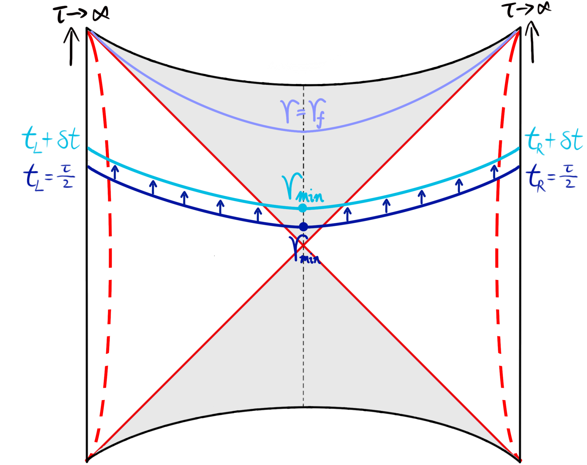
Figure 1: The penrose diagram of the eternal AdS black hole. The curves are the extremal hypersurfaces anchored at $t_{L}=t_{R}=\tau/2$. On the black dashed line $t=0$, we have $\dot{r}|_{r=r_{min}}=0$. When we anchor the boundary time as $\tau\rightarrow\infty$, the extremal hypersurface becomes a constant-$r$ slice, i.e. $r=r_{f}$. This image refers to the FIG. 1 in Ref. Belin:2021bga .

Based on Eq. (10), we can rewrite Eq. (9) as

$$\mathcal{C}=\frac{V_{d-1}}{G_{N}L}\int_{\Sigma}\frac{a(r)^{2}\left(\frac{r}{L}\right)^{2(d-1)}}{\dot{r}}dr.$$ (16)

Using Eq. (14), we can get $\dot{r}=\pm\sqrt{P_{v}^{2}-U(r)}$. In fact, we only have a minimum radius at $\dot{r}=0$ and assume a symmetric configurationas where $t_{L}=t_{R}$, as shown in Fig. 1, so that $\dot{r}$ is positive. On the other hand, we have $U(r_{min})=P_{v}^{2}$, where $r_{min}$ is the minimum radius for the largest generalized volume slice. Therefore, $\dot{r}=\sqrt{U(r_{min})-U(r)}$, and we have

$$\mathcal{C}= \frac{2V_{d-1}}{G_{N}L}\int_{r_{min}}^{r_{\infty}}\frac{a^{2}(r)\left(\frac{r}{L}\right)^{2(d-1)}}{\sqrt{P_{v}^{2}-U(r)}}dr$$

$$= -\frac{2V_{d-1}}{G_{N}L}\int_{r_{min}}^{r_{\infty}}\frac{U(r)}{f(r)\sqrt{U(r_{min})-U(r)}}dr.$$ (17)

On the other hand, according to the ingoing coordinates, we can have

$$\frac{\tau}{2}+r^{*}(r_{\infty})-r^{*}(r_{min}) =\int_{v_{min}}^{v_{\infty}}dv=\int_{r_{min}}^{r_{\infty}}\frac{\dot{v}}{\dot{r}}dr$$

$$=\int_{r_{min}}^{r_{\infty}}dr\left[\frac{1}{f(r)}-\frac{P_{v}}{f(r)\sqrt{P_{v}^{2}+f(r)a(r)^{2}\left(\frac{r}{L}\right)^{2(d-1)}}}\right].$$ (18)

We hope to extract the part containing Eq. (18) from Eq. (17). By following the method provided in Ref. Carmi:2017jqz , we can rewrite Eq. (17) as follows:

$$\mathcal{C}=\frac{2V_{d-1}}{G_{N}L}\int_{r_{min}}^{r_{\infty}}dr\Bigg{[}- \frac{P_{v}^{2}}{f(r)\sqrt{P_{v}^{2}+f(r)a(r)^{2}\left(\frac{r}{L}\right)^{2(d-1)}}}$$

$$+ \frac{\sqrt{P_{v}^{2}+f(r)a(r)^{2}\left(\frac{r}{L}\right)^{2(d-1)}}}{f(r)}+\frac{P_{v}}{f(r)}-\frac{P_{v}}{f(r)}\Bigg{]}.$$ (19)

Therefore, we have

$$\frac{G_{N}L}{2V_{d-1}}\mathcal{C}= \int_{r_{min}}^{r_{\infty}}dr\left[\frac{\sqrt{P_{v}^{2}+f(r)a(r)^{2}\left(\frac{r}{L}\right)^{2(d-1)}}}{f(r)}-\frac{P_{v}}{f(r)}\right]$$

$$+P_{v}\left[\frac{\tau}{2}+r^{*}(r_{\infty})-r^{*}(r_{min})\right].$$ (20)

Next, we can take the time derivative of Eq. (20):

$$\frac{G_{N}L}{2V_{d-1}}\frac{d\mathcal{C}}{d\tau}= \frac{dP_{v}}{d\tau}\int_{r_{min}}^{r_{\infty}}dr\left[\frac{P_{v}}{f(r)\sqrt{P_{v}^{2}+f(r)a(r)^{2}\left(\frac{r}{L}\right)^{2(d-1)}}}-\frac{1}{f(r)}\right]$$

$$+\frac{dP_{v}}{d\tau}\left[\frac{\tau}{2}+r^{*}(r_{\infty})-r^{*}(r_{min})\right]+\frac{P_{v}}{2}.$$ (21)

We notice that the same term as in Eq. (18) appears in Eq. (21), which can greatly simplify the equation, that is

$$\frac{d\mathcal{C}}{d\tau}=\frac{V_{d-1}}{G_{N}L}P_{v}.$$ (22)

Therefore, the growth rate of the complexity is proportional to the conserved momentum $P_{v}$. Due to $r^{*}=-\int_{r}^{\infty}\frac{dr^{\prime}}{f(r^{\prime})}$, we can get the expression of the boundary time by Eq. (18):

$$\tau= -2\int_{r_{min}}^{\infty}dr\frac{P_{v}}{f(r)\sqrt{P_{v}^{2}+f(r)a(r)^{2}\left(\frac{r}{L}\right)^{2(d-1)}}}$$

$$= -2\int_{r_{min}}^{\infty}dr\frac{P_{v}}{f(r)\sqrt{P_{v}^{2}-U(r)}}.$$ (23)

When $\tau\rightarrow\infty$, we let the $U(r_{f})=P_{\infty}$, so we have

$$\frac{d\mathcal{C}}{d\tau}\bigg{|}_{\tau\rightarrow\infty}=\frac{V_{d-1}}{G_{N}L}P_{\infty}.$$ (24)

3 Different Gravitational Observables and Turning Time

There are some examples of $a(r)$ presented in Ref. Jorstad:2023kmq . In this section, we expand on their examples and consider the turning time in each other. We also use the Weyl tensor for the bulk spacetime to construct the gravitational observable on the codimension-one extremal slice $\Sigma$. That is

$$a(r)= 1+\sum_{j=1}^{N}(-1)^{j}\lambda_{j}(L^{4}C^{2})^{j},$$ (25)

$$C^{2}\equiv R_{\mu\nu\sigma\rho}R^{\mu\nu\sigma\rho}-\frac{4}{d-1}R_{\mu\nu}R^{\mu\nu}+\frac{2}{d(d-1)}R=d(d-1)^{2}(d-2)\frac{r_{h}^{2d}}{L^{4}r^{2d}},$$ (26)

where $C^{2}\equiv C_{\mu\nu\sigma\rho}C^{\mu\nu\sigma\rho}$ denotes the square of the Weyl tensor for the bulk spacetime, $\lambda_{j}$ are dimensionless coupling constants, and $j=1,2,\cdots,N$. To simplify the calculation, we set $\tilde{\lambda}_{j}=[d(d-1)^{2}(d-2)]^{j}\lambda_{j}$. After this substitution, $a(r)$ can be rewritten as

$$a(r)=1+\sum_{j=1}^{N}(-1)^{j}\tilde{\lambda}_{j}\left(\frac{r_{h}}{r}\right)^{2dj}.$$ (27)

When all $\lambda_{j}=0$, we have $a(r)=1$, which corresponds to the CV proposal. The case of $N=1$ was discussed in Ref. Belin:2021bga . We begin our analysis with $N=2$, i.e.,

$$a(r)=1-\tilde{\lambda}_{1}\left(\frac{r_{h}}{r}\right)^{2d}+\tilde{\lambda}_{2}\left(\frac{r_{h}}{r}\right)^{4d}.$$ (28)

It was chosen in Ref. Jorstad:2023kmq to make the extreme surface approaches the singularity. Then, we can obtain the expression of the effective potential, i.e.,

$$U(r)=-r^{-d}\left(\frac{r}{L}\right)^{2d}(r^{d}-r_{h}^{d})\left[1-\left(\frac{r_{h}}{r}\right)^{2d}\tilde{\lambda}_{1}+\left(\frac{r_{h}}{r}\right)^{4d}\tilde{\lambda}_{2}\right]^{2}.$$ (29)

We consider the case of $d=3$ and choose appropriate value of the coupling parameter $\lambda_{j}$ as shown in Fig. 2. In the red area, $U(r)$ gives two peaks, and their values graualdly decrease from left to right. According to Eq. (17), we can obtain the expression for the generalized volume, which is given by

$$V_{gen}=V_{d-1}\int_{r_{min}}^{r_{\infty}}\frac{a^{2}(r)\left(\frac{r}{L}\right)^{2(d-1)}}{\sqrt{Pv^{2}-U(r)}}dr.$$ (30)

By calculating the generalized volume, we can observe its correspondence with $P_{v}$ as shown in the right image of Fig. 3. When we select the appropriate value of $\lambda$ to construct the $U(r)$ as shown in the left image of Fig. 2, there are two local maxima of the effective potential. Equation (22) tells us that a higher peak corresponds to a larger growth rate of the generalized volume-complexity. Therefore, at a very late time, the generalized volume corresponding to the peak on the left must be bigger than that of the right. Interestingly, as shown in the left image of Fig. 3, the shorter peak corresponds to a larger generalized volume over a significant range. Consequently, there must be a moment when the generalized volumes corresponding to the left and right peaks are equal, and after that, the relative size relationship between these two will reverse. We refer to this moment as the turning timeWang:2023eep .

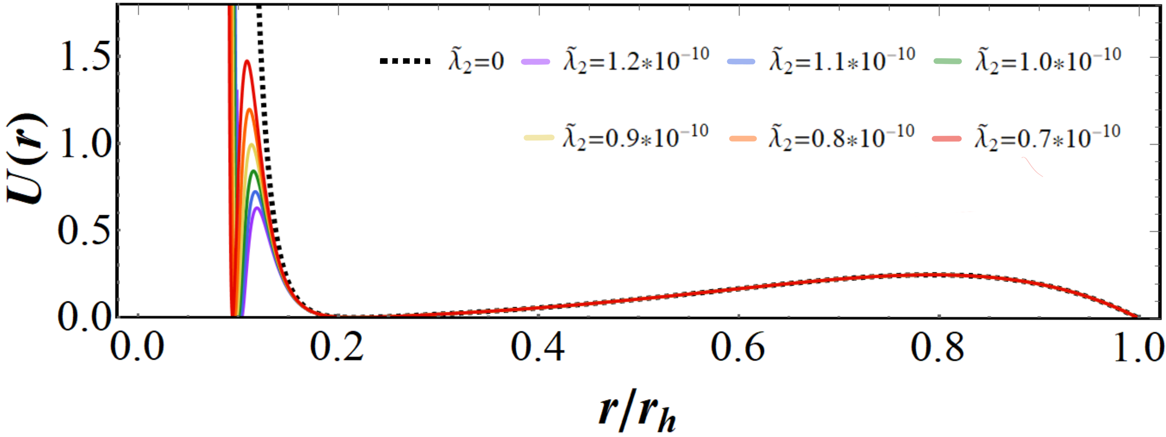
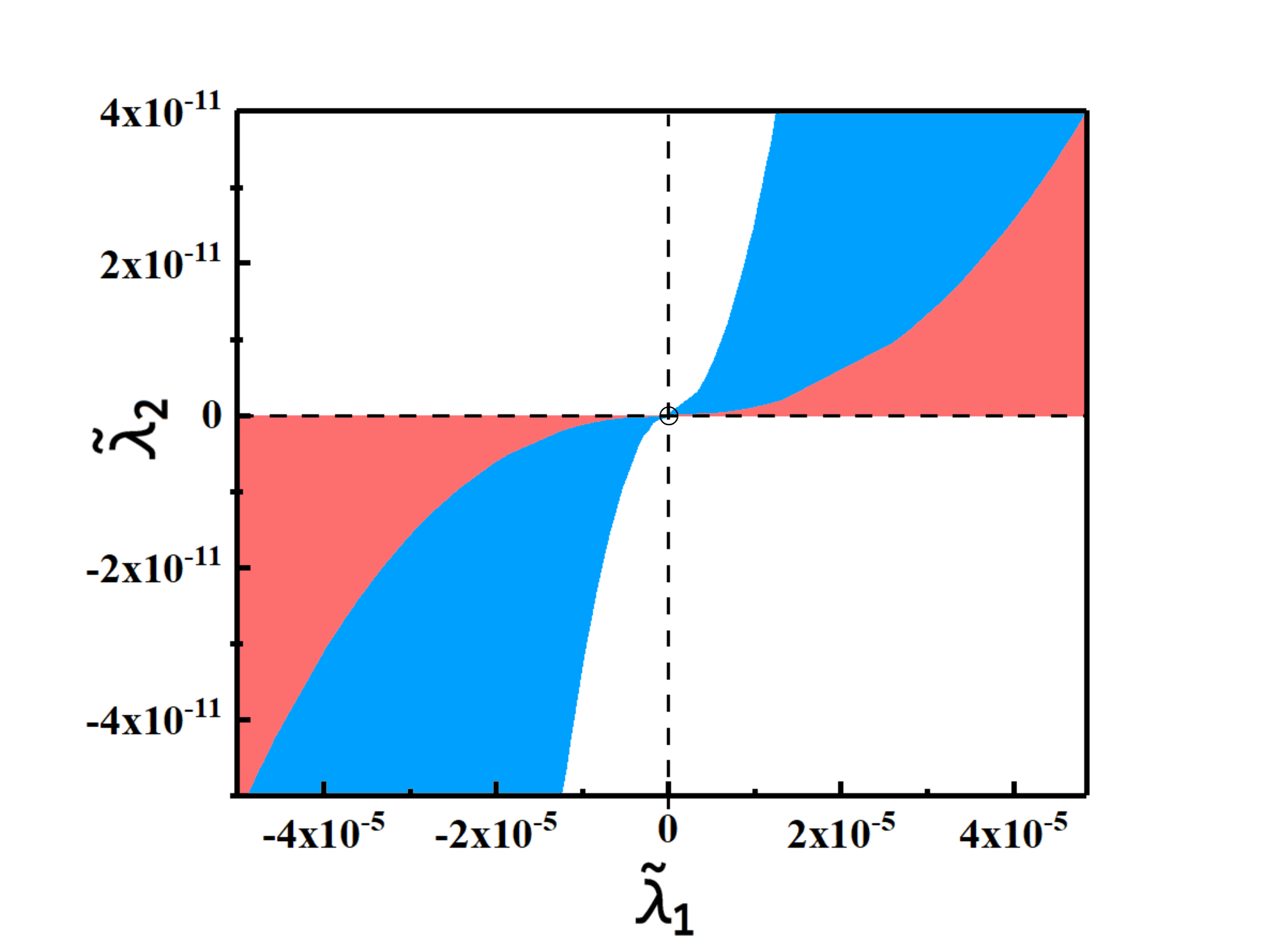
Figure 2: Left: The colorful curves represent the $U(r)$ with $\tilde{\lambda}_{1}=10^{-4}$ and different values of $\tilde{\lambda}_{2}$, and the black dotted line corresponds to the CV proposal. Right: The parameter space of $\tilde{\lambda}_{1}$ and $\tilde{\lambda}_{2}$. In the red area, the effective potential has two local maxima, and the left one is larger than the right one. In the blue area, there are also two local maxima, but the local maxima on the right is greater than the one on the left. In the remaining white area, there is only one or possibly no local maximum.

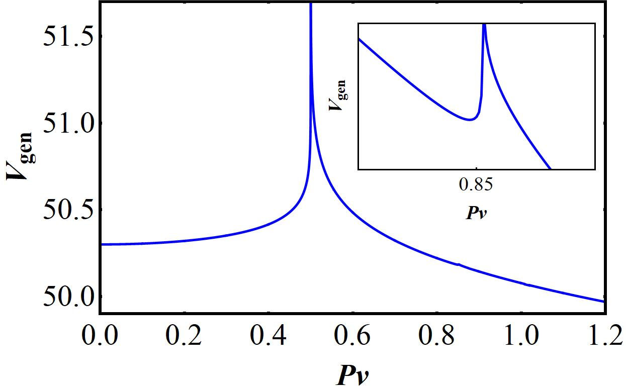
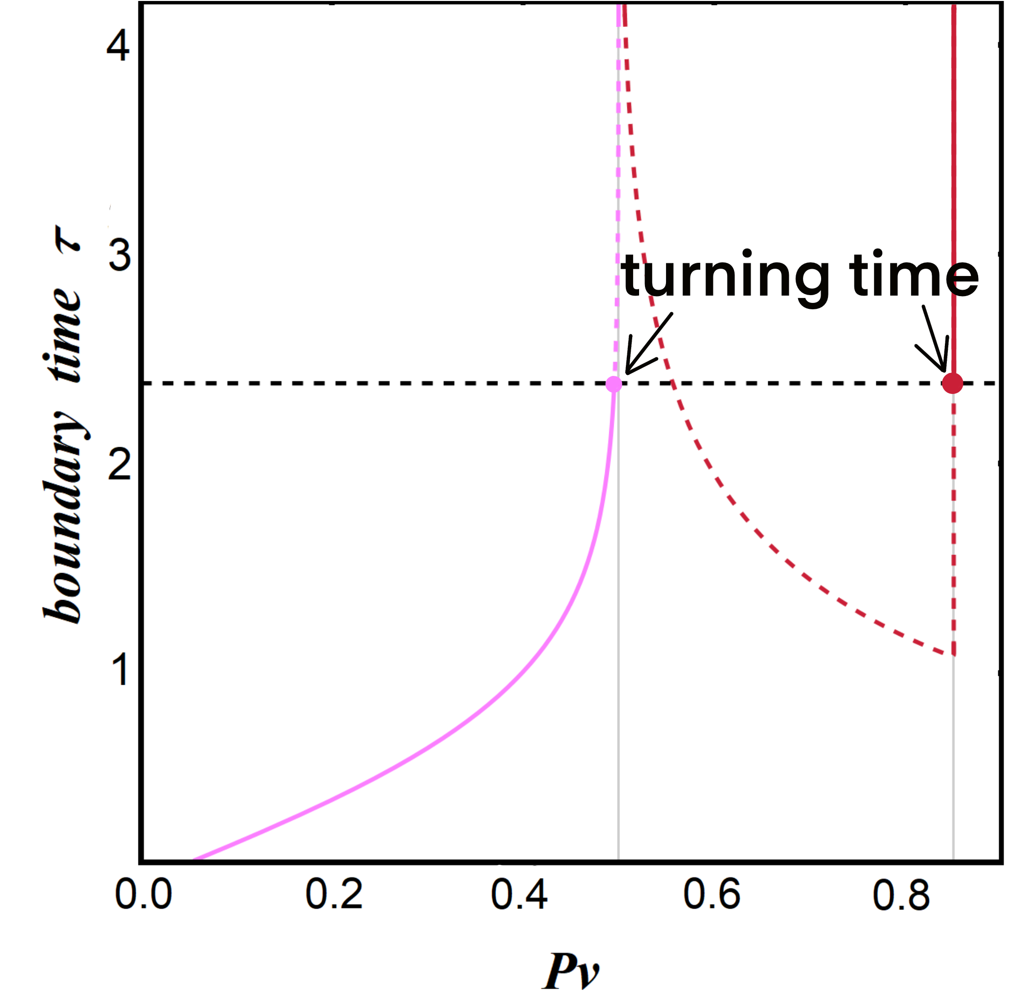
Figure 3: Left:The generalized volume of the planar AdS black hole with $d=3,~{}\frac{r_{h}}{L}=1,~{}\tilde{\lambda}_{1}=10^{-4},~{}\tilde{\lambda}_{2}=1.1*10^{-10}$. The part outside the horizon grows linearly with $r$ and diverges at infinity, we just cutoff it at $r=10r_{h}$. Right: The relation between the boundary time $\tau$ and the conserved momentum $P_{v}$ using the parameters mentioned above. The two solid grey lines represent the two local maxima of $U(r)$, i.e., $U(r_{f})$. The pink curve corresponds to the right peak, and the red curve corresponds to the left one. Both the pink and red solid lines represent larger generalized volumes at the corresponding boundary time, while the dotted lines are the opposite.

By selecting different values of $\tilde{\lambda}_{1}$ and $\tilde{\lambda}_{2}$, we can get the corresponding relationship between the parameters and the turning time, as shown in Fig. 4. In another paper, we investigated the turning time for the four-dimensional RN-AdS black hole Wang:2023eep .

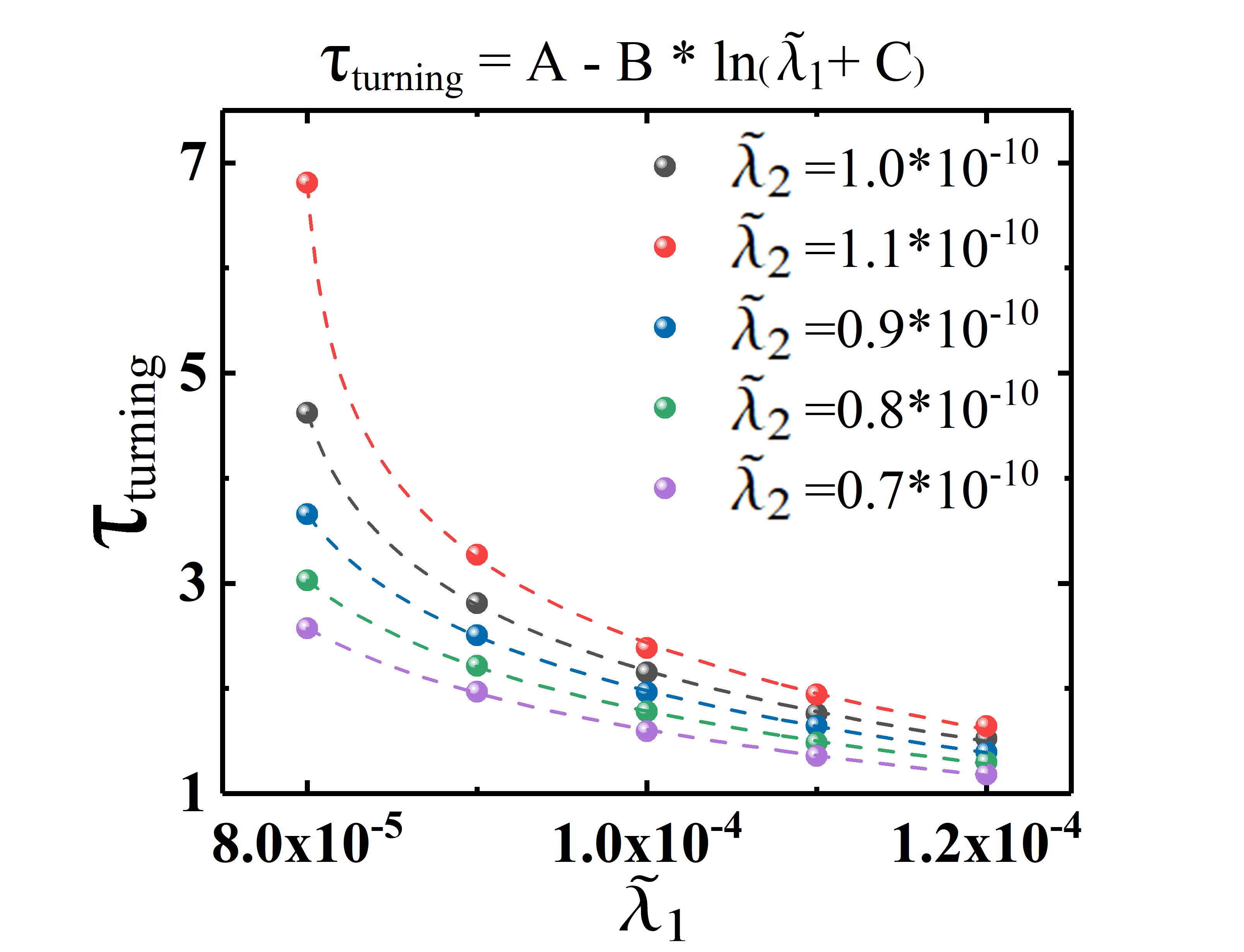
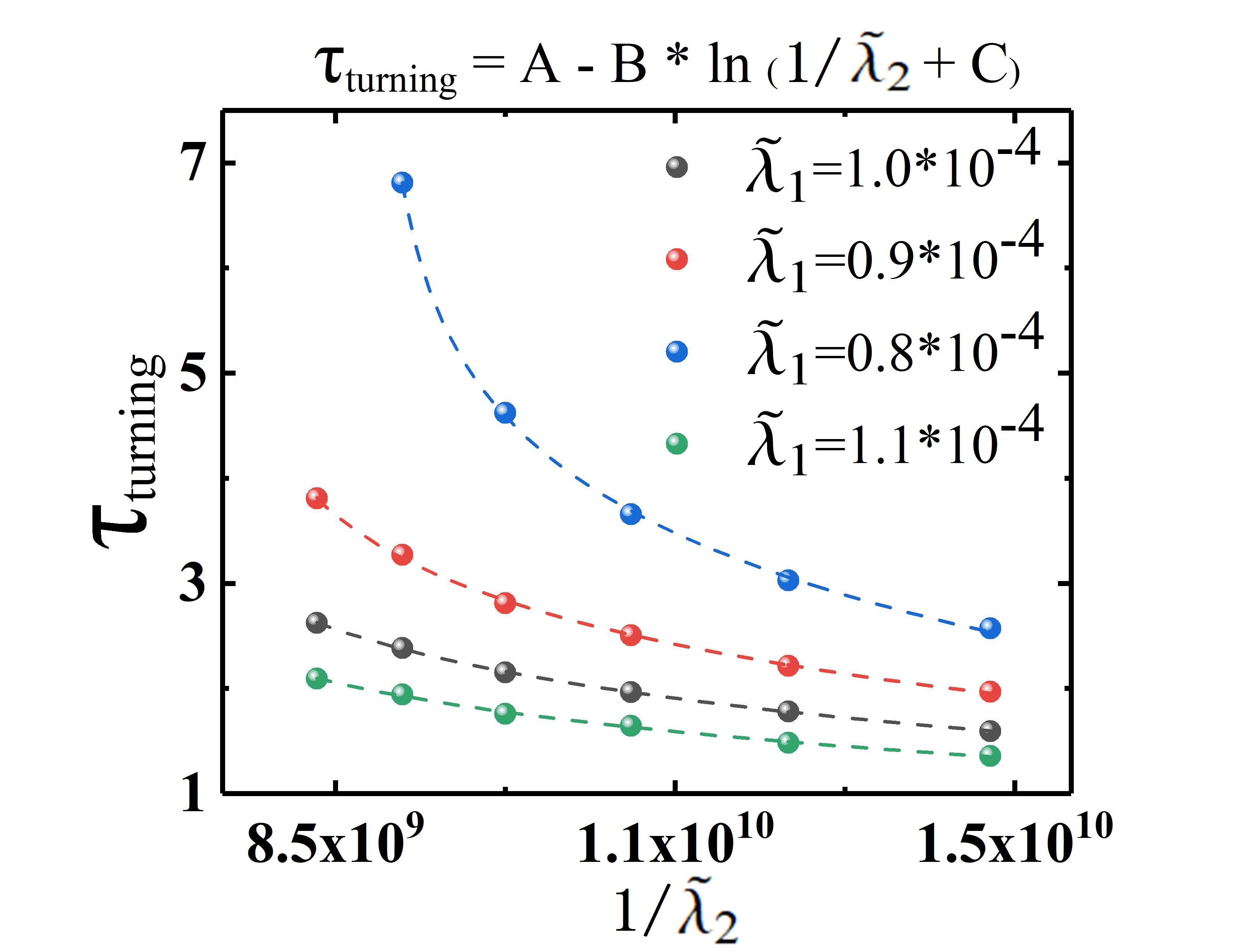
Figure 4: The fitting of turning time on $\tilde{\lambda}_{1}$ and $\tilde{\lambda}_{2}$.

We discoverd that the turning time has a logarithmic dependence on its parameter, and we have determined the fitting function to be given by

$$\tau_{turning}= a_{1}-b_{1}\ln(\tilde{\lambda}_{1}+c_{1}),$$ (31)

$$\tau_{turning}= a_{2}-b_{2}\ln(\tilde{\lambda}_{2}+c_{2}),$$ (32)

where $a_{i}$, $b_{i}$, and $c_{i}$ are the fitting values. Among them, $a_{i}$ and $b_{i}$ have dimensions of length, while $c_{i}$ are dimensionless constants.

Similarly, we can also consider polynomials with three monomials or even more. Choosing $N=3$, we can get

$$a(r) =1-\tilde{\lambda}_{1}\left(\frac{r}{L}\right)^{2d}+\tilde{\lambda}_{2}\left(\frac{r}{L}\right)^{4d}-\tilde{\lambda}_{3}\left(\frac{r}{L}\right)^{6d},$$ (33)

$$U(r) =-r^{-d}\left(\frac{r}{L}\right)^{2d}(r^{d}-r_{h}^{d})\left[1-\left(\frac{r_{h}}{r}\right)^{2d}\tilde{\lambda}_{1}+\left(\frac{r_{h}}{r}\right)^{4d}\tilde{\lambda}_{2}-\left(\frac{r_{h}}{r}\right)^{6d}\tilde{\lambda}_{3}\right]^{2}.$$ (34)

As before, we continue to consider the planer black hole in $(3+1)$-dimensional spacetime. Choosing different values of the parameters, we may have from $0$ to $3$ local maxima of the effective potential, as shown in the left image of Fig. 5. In this case, there are three growth rates at late time. However, the number of turning times does not necessarily have to be two, as shown in the right image of Fig. 5.

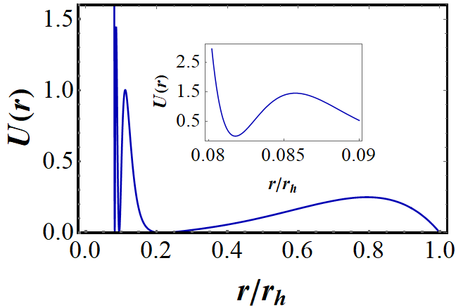
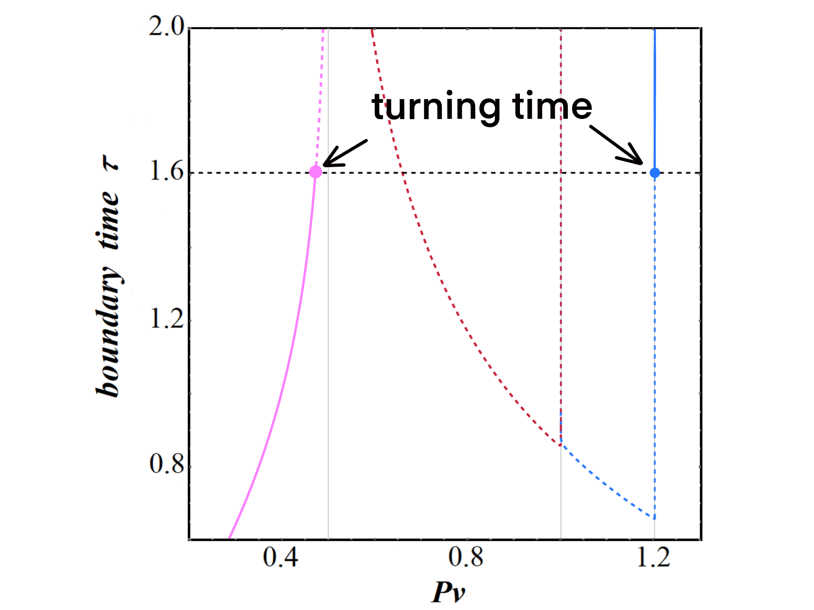
Figure 5: Left: The image of the effective potential $U(r)$ with $L=1$, $\tilde{\lambda}_{1}=10^{-4}$, $\tilde{\lambda}_{2}=10^{-10}$ and $\tilde{\lambda}_{3}=2.1*10^{-17}$. Right: The relation between the boundary time $\tau$ and the conserved momentum $P_{v}$ using the parameters mentioned above. The three solid grey lines represent the three local maxima of $U(r)$, i.e., $U(r_{f})$. The pink, red and blue curves correspond to the right, middle and left peaks respectively. Both the pink and blue solid lines represent larger generalized volumes at the corresponding boundary time, while the dotted lines are the opposite.

The highest peak is so steep that the middle peak corresponds to a generalized volume that can never be the largest. On the other hand, if we select more extreme parameters such that the heights of the two peaks on the left and middle are very close to each other, we can identify a second turning time, as shown in Fig. 6.

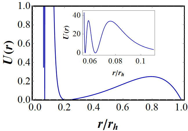
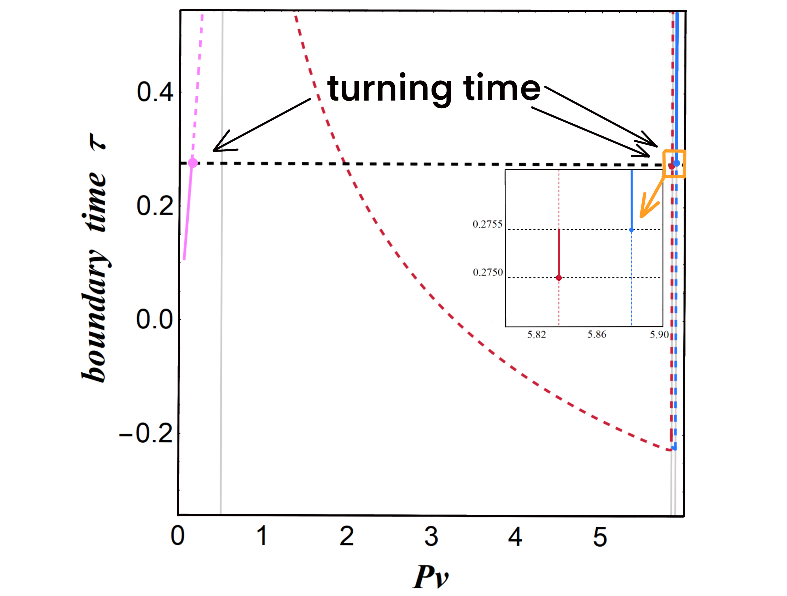
Figure 6: Left: The image of the effective potential $U(r)$ with $L=1$, $\tilde{\lambda}_{1}=10^{-4}$, $\tilde{\lambda}_{2}=10^{-9}$ and $\tilde{\lambda}_{3}=2.135*10^{-17}$. Right: The relation between the boundary time $\tau$ and the conserved momentum $P_{v}$ using the parameters mentioned above. The three solid grey lines represent the three local maxima of $U(r)$, i.e., $U(r_{f})$. The pink, red and blue curves correspond to the right, middle and left peaks, respectively. The pink, red and blue solid lines represent larger generalized volumes at the corresponding boundary time, while the dotted lines are the opposite.

The emergence of turning time shows that perhaps the growth rate of complexity is not smooth, but rather suddenly change at a certain moment. This phenomenon may imply that there are phase transitions, and means that the shortest evolution path from the reference state to the target state in quantum computing complexity may experience a sudden jump. Similar phase transitions have also been observed in circuit complexity Roca-Jerat:2023mjs .

4 Holographic Complexity for Charged BTZ Black Holes

In this section, we consider the generalized volume-complexity for the charged BTZ black holes by using gravitational observable constructed with the electromagnetic field tensor. Let’s first consider the charged BTZ black hole, whose metrics are provided in Ref. Banados:1992wn ; Martinez:1999qi ,

$$ds^{2} =-f(r)dt^{2}+\frac{dr^{2}}{f(r)}+r^{2}d\theta^{2},$$

$$f(r) =-M+\frac{r^{2}}{L^{2}}-\pi Q^{2}\ln{\frac{r}{L}}\equiv\frac{(r^{2}-r_{+}^{2})(r^{2}-r_{-}^{2})}{L^{2}r^{2}}.$$ (35)

The metric is asymptotically AdS₃ with radius $L$. In the usual convention, we set $8G_{N}\equiv 1$, where $G_{N}$ is the Newton’s constant. The mass and the charge of the solution are denoted by $M$ and $Q$, and can be expressed in terms of the parameters $r_{\pm}$:

$$M= \frac{r_{+}^{2}\ln{\frac{r_{-}}{L}}-r_{-}^{2}\ln{\frac{r_{+}}{L}}}{L^{2}\ln{\frac{r_{-}}{r_{+}}}},$$ (36)

$$Q^{2}= \frac{r_{+}^{2}-r_{-}^{2}}{\pi L^{2}\ln{\frac{r_{+}}{r_{-}}}}.$$ (37)

We can also rewrite the metric into the ingoing Eddington-Finkelstein coordinates, that is

$$ds^{2}=-f(r)dv^{2}+2dvdr+r^{2}d\phi^{2}.$$ (38)

The generalized volume-complexity can be represented by

$$\mathcal{C}=2\pi\int d\sigma~{}r~{}\sqrt{2\dot{v}\dot{r}-f(r)\dot{v}^{2}}~{}a(r)\equiv\frac{2\pi}{G_{N}L}\int_{\Sigma}d\sigma\mathcal{L}(r,\dot{v},\dot{r}).$$ (39)

Obviously, the gauge given by Eq. (10) becomes

$$\sqrt{-f(r)\dot{v}^{2}+2\dot{v}\dot{r}}=a(r){r}.$$ (40)

We can just write down its effective potential, complexity, and complexity growth rate:

$$U(r)= -f(r)a^{2}(r)r^{2},$$ (41)

$$\mathcal{C}= -\frac{4\pi}{G_{N}L}\int_{r_{min}}^{\infty}\frac{U(r)}{f(r)\sqrt{U(r_{min})-U(r)}}dr,$$ (42)

$$\frac{d\mathcal{C}}{d\tau}= \frac{2\pi}{G_{N}L}P_{v}.$$ (43)

It is well know that the Weyl tensor is always zero when $d=2$, so we need to look for other non-trivial scalar functions. In this situation, we choose $a(r)=1-\lambda L^{2}F_{\mu\nu}F^{\mu\nu}$, where $F_{\mu\nu}F^{\mu\nu}=-2\frac{Q^{2}}{r^{2}}$, i.e,

$$U(r)=-\frac{1}{L^{2}}(r^{2}-r_{+}^{2})(r^{2}-r_{-}^{2})\left(1+\frac{2(r_{+}^{2}-r_{-}^{2})\lambda}{\pi r^{2}\ln{\frac{r_{-}}{r_{+}}}}\right)^{2}.$$ (44)

Of course, we can use this configuration to analyze all other charged black holes.

In this case, we can still find a series of $\lambda$, $Q$ and $M$ such that $U(r)$ has more than one local maxima between $r_{-}$ and $r_{+}$, the one with smaller $r$ is also larger. The parameter space is shown in Fig. 7.

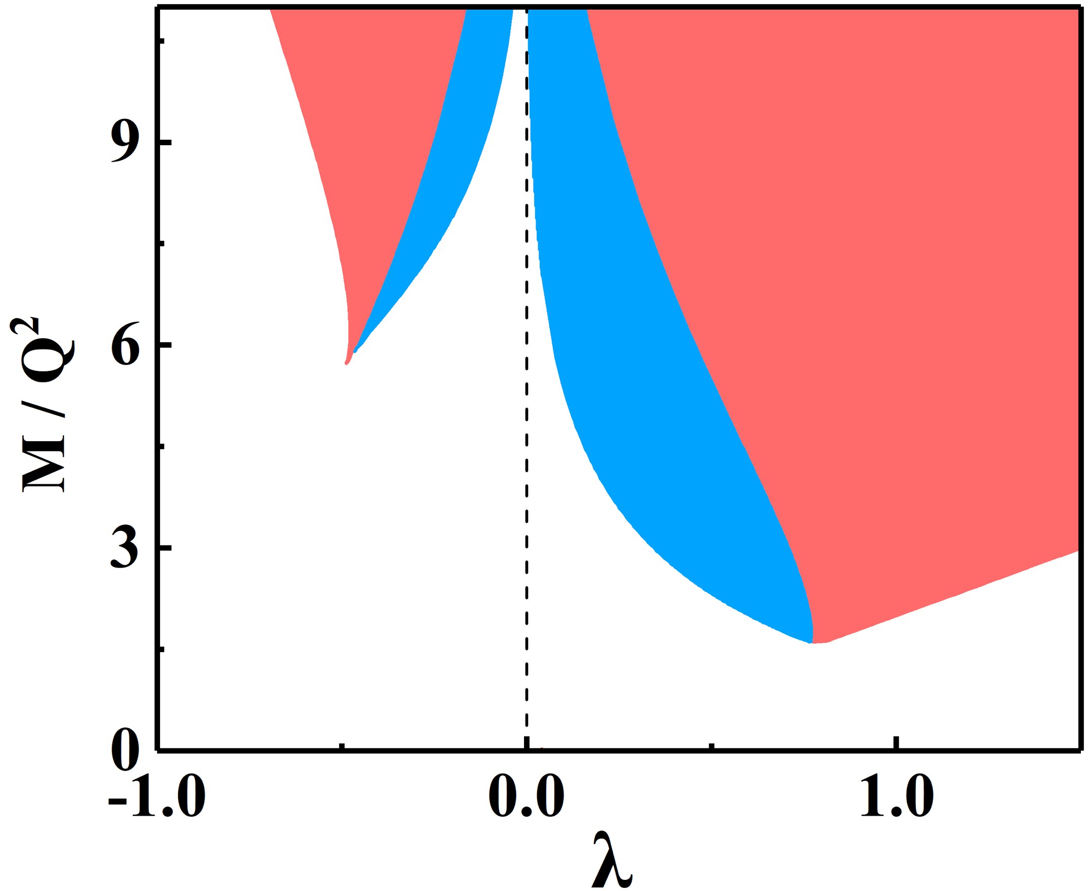
Figure 7: The parameter space of the effective potential $U(r)$ between the two horizons of the charged BTZ black hole. In the red area, there are two local maxima that decrease from left to right. In the blue area, there are also two local maxima, but the local maximum on the right is greater than the one on the left. In the remaining white area, there is only one local maximum.

In the analysis that follows, we only consider the parameters that fall within the red areas, where we have two local maxima that describe from left to right. As before, we consider their turning time. For the example shown in Fig. 8, the boundary time and turning time can be reflected in Fig. 9.

Figure 8: The effective potential defined in Eq.(44). In this situation, we may have 1 or 2 local maxima of the effective potential for different parameters. When the number of the local maxima is one, the result is similar to the CV proposal. Therefore, we only consider the case of two local maxima. Left: the shape of the effective potential for $\lambda=0.2$, $r_{-}=0.2r_{+}$, $L=1$, and $r_{+}=1$. There are two local maxima and the local minimum between them is zero. Right: the shape of the effective potential for $\lambda=-0.6$, $r_{-}=0.2r_{+}$, $L=1$, and $r_{+}=1$. There are also two local maxima but the minimum between them does not reach zero. Whether the local minimum is zero depends only on the positive or negative of $\lambda$.

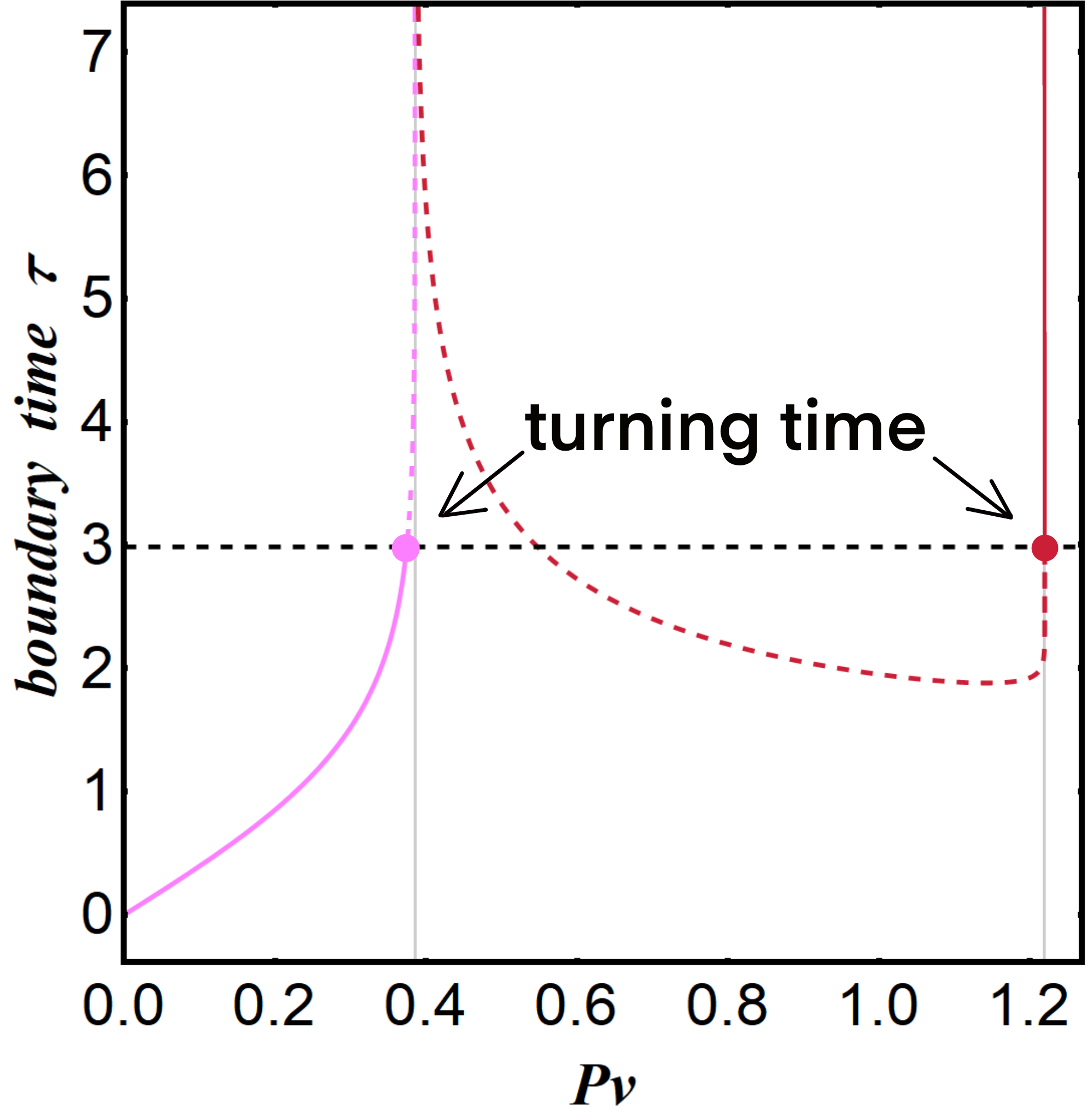
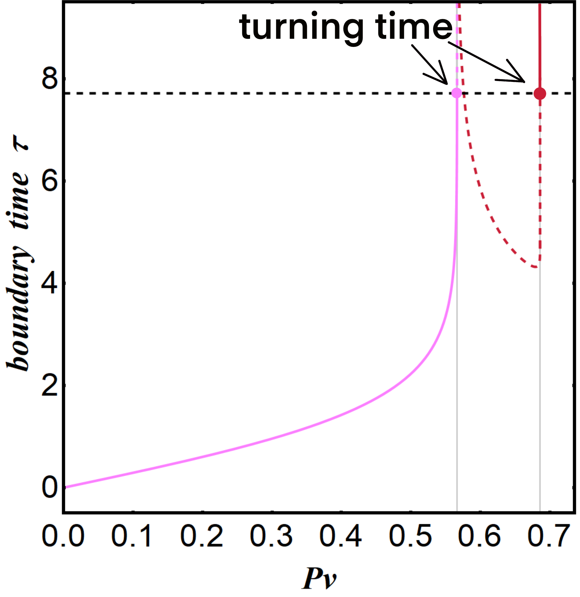
Figure 9: The relation between the boundary time $\tau$ and the conserved momentum $P_{v}$. Left: $\lambda=0.2$, $r_{-}=0.5r_{+}$, $L=1$ and $r_{+}=1$. Right: $\lambda=0.001$, $r_{-}=0.135r_{+}$, $L=1$ and $r_{+}=1$.

We fix $r_{+}=L=1$ and choose different $\frac{M}{Q^{2}}$ or $\lambda$ to construct a series of $U(r)$ as shown in Fig. 10, where we only consider the case that the effective potential has two loacl maxima. It is worth mentioning that when we fix $r_{+}$ and $L$, $r_{-}$ varies monotonically with $\frac{M}{Q^{2}}$. Therefore, we can describe the change of $\frac{M}{Q^{2}}$ by changing $r_{-}$ during our calculations, as shown in the right figure of Fig. 10. In the subsequent calculations, we will consistently determine the value of $\frac{M}{Q^{2}}$ by inversely solving it with a fixed $r_{-}$.

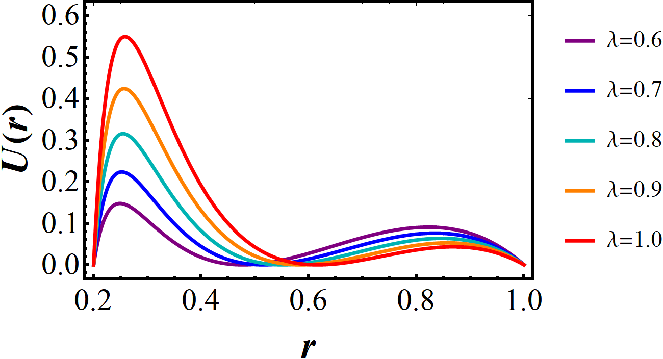
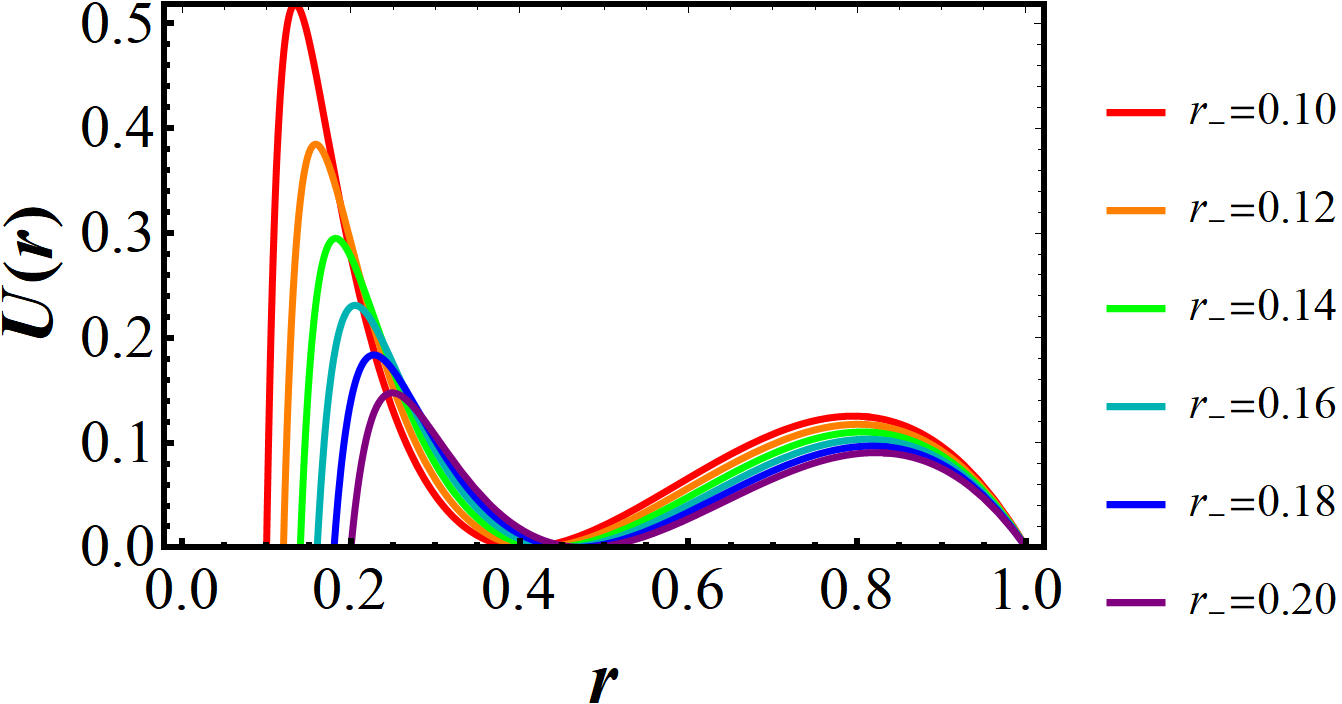
Figure 10: Left: the shape of the effective potential for $\lambda=0.6$ to $1.0$, $L=r_{+}=1$, and $r_{-}=0.2r_{+}$. Right: the shape of the effective potential for $r_{-}=0.1r_{+}$ to $0.2r_{+}$, $L=r_{+}=1$, and $\lambda=0.6$.

There are a series of turning times that can be found. The turning time of the complexity is still logarithmic with its parameter as shown in Fig. 11:

$$\tau_{turning}= A_{QM}-B_{QM}\ln\left(\frac{M}{Q^{2}}+C_{QM}\right),$$

$$\tau_{turning}= A_{\lambda}-B_{\lambda}\ln(\lambda+C_{\lambda}),$$ (45)

where $A$, $B$ and $C$ are the fitting values. Among them, $A$ and $B$ have length dimensions, and $C$ is a dimensionless constant. This conclusion is consistent with the result of considering the square of the Weyl tensor for the planar AdS black hole in Sec. 2.

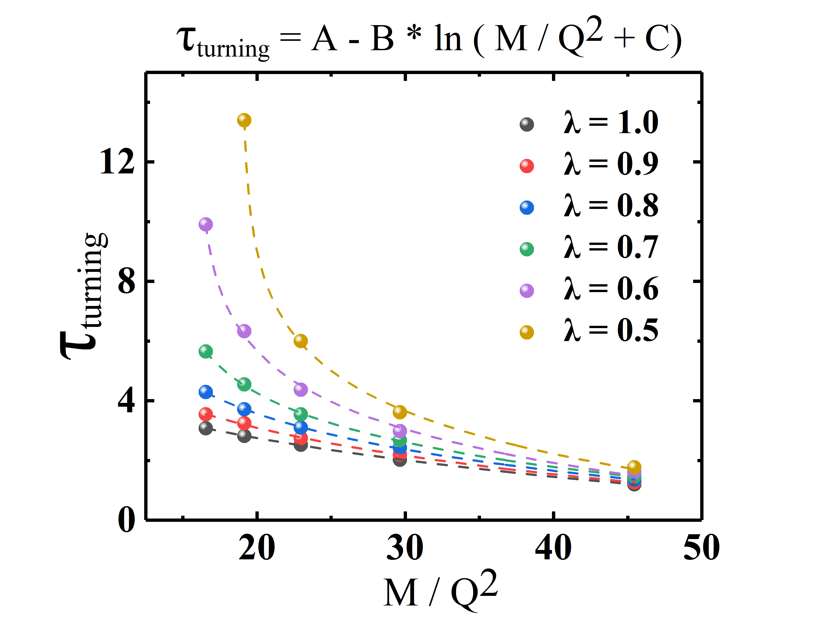
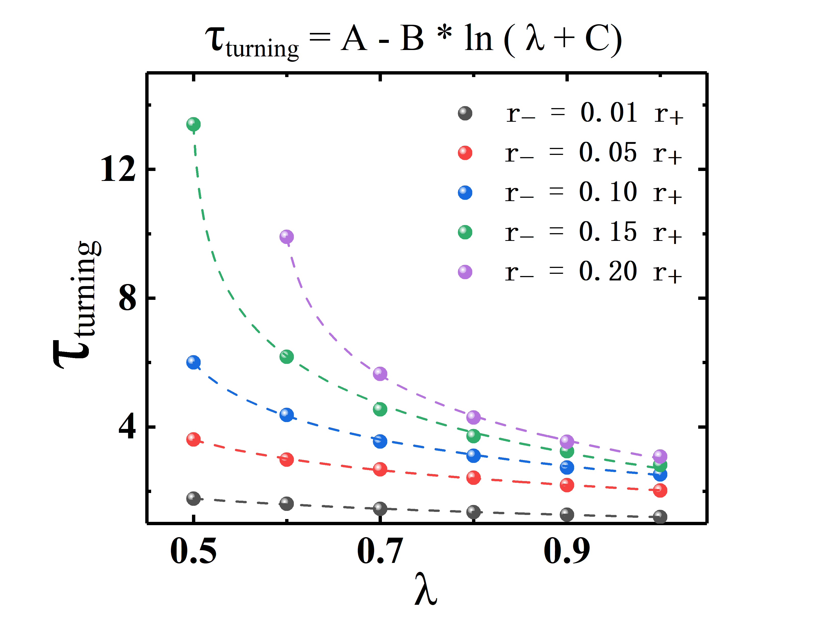
Figure 11: The fitting of turning time on $\lambda$ and $M/Q^{2}$.

5 Discussion

In this paper, we calculated of the holographic complexity for the planar AdS black hole and the charged BTZ black hole. Additionally, we derived the expressions for complexity, Eq. (17), and the growth rate of complexity, Eq. (22). The growth rate of complexity is directly proportional to the conserved momentum $P_{v}$. To construct various gravitational observables, we used some different scalar functions $a(r)$ like $1+\sum_{j=1}^{N}(-1)^{j}\lambda_{j}(L^{4}C^{2})^{j}$ or $1-\lambda L^{2}F_{\mu\nu}F^{\mu\nu}$. Through this process, we discovered that the effective potentials exhibit diverse behaviors depending on the choice of $a(r)$, which corresponds to different behaviors in the growth rate of complexity.

In the case we analyzed, there are two or multiple local maxima for the effective potential. Through numerical integration to inverse solve the boundary times with Eq. (23), we observed that in the $P_{v}-\tau$ diagram, multiple $P_{v}$ values can intersect at the same boundary time $\tau$. It means there are multiple generalized volumes that anchor to the same boundary time. We chose the largest generalized volume as the dual of the complexity. However, the relative sizes of the generalized volumes are not fixed, the smaller one would “surpass” at a certain moment. We called the moment as the turning time. Further, we found that the turning time has a logarithmic relationship with the parameters.

Finally, it should be pointed out that we can also consider a modified gravitational black hole model with a holographic dual, like the Gauss-Bonnet-AdS black hole. For this case, we can choose the flowing more natural scalar function and the coupling constant of the equilibrium dimension:

$$a(r)= 1+\sum_{j=1}^{N}(-1)^{j}\lambda_{j}(\alpha^{2}R_{GB}^{2})^{j},$$ (46)

$$R_{GB}^{2}\equiv R^{2}-4R_{\mu\nu}R^{\mu\nu}+R_{\mu\nu\sigma\rho}R^{\mu\nu\sigma\rho},$$ (47)

where $R_{GB}$ is the Gauss-Bonnet term and the $\alpha$ is its coupling constant. We can build on this to study the holographic complexity of modified gravitational black holes.

References

- (1) J. M. Maldacena, “The Large N limit of superconformal field theories and supergravity,” Adv. Theor. Math. Phys. 2, 231-252 (1998) [arXiv:hep-th/9711200 [hep-th]].
- (2) J. M. Maldacena, “TASI 2003 lectures on AdS / CFT,” [arXiv:hep-th/0309246 [hep-th]].
- (3) J. Maldacena and L. Susskind, “Cool horizons for entangled black holes,” Fortsch. Phys. 61, 781-811 (2013) [arXiv:1306.0533 [hep-th]].
- (4) L. Susskind, “Copenhagen vs Everett, Teleportation, and ER=EPR,” Fortsch. Phys. 64, no.6-7, 551-564 (2016) [arXiv:1604.02589 [hep-th]].
- (5) L. Susskind, “Computational Complexity and Black Hole Horizons,” Fortsch. Phys. 64, 24-43 (2016) [arXiv:1403.5695 [hep-th]].
- (6) D. Stanford and L. Susskind, “Complexity and Shock Wave Geometries,” Phys. Rev. D 90, no.12, 126007 (2014) [arXiv:1406.2678 [hep-th]].
- (7) L. Susskind, “Entanglement is not enough,” Fortsch. Phys. 64, 49-71 (2016) [arXiv:1411.0690 [hep-th]].
- (8) S. H. Shenker and D. Stanford, “Black holes and the butterfly effect,” JHEP 03, 067 (2014) [arXiv:1306.0622 [hep-th]].
- (9) D. A. Roberts, D. Stanford and L. Susskind, “Localized shocks,” JHEP 03, 051 (2015) [arXiv:1409.8180 [hep-th]].
- (10) A. R. Brown, D. A. Roberts, L. Susskind, B. Swingle and Y. Zhao, “Holographic Complexity Equals Bulk Action?,” Phys. Rev. Lett. 116, no.19, 191301 (2016) [arXiv:1509.07876 [hep-th]].
- (11) A. R. Brown, D. A. Roberts, L. Susskind, B. Swingle and Y. Zhao, “Complexity, action, and black holes,” Phys. Rev. D 93, no.8, 086006 (2016) [arXiv:1512.04993 [hep-th]].
- (12) J. Couch, W. Fischler and P. H. Nguyen, “Noether charge, black hole volume, and complexity,” JHEP 03, 119 (2017) [arXiv:1610.02038 [hep-th]].
- (13) L. C. Qu, H. Y. Jiang and Y. X. Liu, “Chaos and multifold complexity for an inverted harmonic oscillator,” JHEP 12, 065 (2022) [arXiv:2211.04317 [quant-ph]].
- (14) L. C. Qu, J. Chen and Y. X. Liu, “Chaos and complexity for inverted harmonic oscillators,” Phys. Rev. D 105, no.12, 126015 (2022) [arXiv:2111.07351 [hep-th]].
- (15) D. Carmi, R. C. Myers and P. Rath, “Comments on Holographic Complexity,” JHEP 03, 118 (2017) [arXiv:1612.00433 [hep-th]].
- (16) D. Carmi, S. Chapman, H. Marrochio, R. C. Myers and S. Sugishita, “On the Time Dependence of Holographic Complexity,” JHEP 11, 188 (2017) [arXiv:1709.10184 [hep-th]].
- (17) S. Chapman, H. Marrochio and R. C. Myers, “Holographic complexity in Vaidya spacetimes. Part I,” JHEP 06, 046 (2018) [arXiv:1804.07410 [hep-th]].
- (18) S. Chapman, H. Marrochio and R. C. Myers, “Holographic complexity in Vaidya spacetimes. Part II,” JHEP 06, 114 (2018) [arXiv:1805.07262 [hep-th]].
- (19) B. Swingle and Y. Wang, “Holographic Complexity of Einstein-Maxwell-Dilaton Gravity,” JHEP 09, 106 (2018) [arXiv:1712.09826 [hep-th]].
- (20) Z. Fu, A. Maloney, D. Marolf, H. Maxfield and Z. Wang, “Holographic complexity is nonlocal,” JHEP 02, 072 (2018) [arXiv:1801.01137 [hep-th]].
- (21) R. G. Cai, S. M. Ruan, S. J. Wang, R. Q. Yang and R. H. Peng, “Action growth for AdS black holes,” JHEP 09, 161 (2016) [arXiv:1606.08307 [gr-qc]].
- (22) R. Q. Yang and S. M. Ruan, “Comments on Joint Terms in Gravitational Action,” Class. Quant. Grav. 34, no.17, 175017 (2017) [arXiv:1704.03232 [gr-qc]].
- (23) W. D. Guo, S. W. Wei, Y. Y. Li and Y. X. Liu, “Complexity growth rates for AdS black holes in massive gravity and gravity,” Eur. Phys. J. C 77, no.12, 904 (2017) [arXiv:1703.10468 [gr-qc]].
- (24) J. Couch, S. Eccles, T. Jacobson and P. Nguyen, “Holographic Complexity and Volume,” JHEP 11, 044 (2018), [arXiv:1807.02186 [hep-th]].
- (25) M. Zhang, C. Fang and J. Jiang, “Holographic complexity of rotating black holes with conical deficits,” Phys. Lett. B 838, 137691 (2023) [arXiv:2212.05902 [hep-th]].
- (26) L. Susskind and Y. Zhao, “Switchbacks and the Bridge to Nowhere,” [arXiv:1408.2823 [hep-th]].
- (27) S. Chapman, H. Marrochio and R. C. Myers, “Complexity of Formation in Holography,” JHEP 01, 062 (2017) [arXiv:1610.08063 [hep-th]].
- (28) R. G. Cai, M. Sasaki and S. J. Wang, “Action growth of charged black holes with a single horizon,” Phys. Rev. D 95, no.12, 124002 (2017) [arXiv:1702.06766 [gr-qc]].
- (29) Y. S. An and R. H. Peng, “Effect of the dilaton on holographic complexity growth,” Phys. Rev. D 97, no.6, 066022 (2018) [arXiv:1801.03638 [hep-th]].
- (30) K. Goto, H. Marrochio, R. C. Myers, L. Queimada and B. Yoshida, “Holographic Complexity Equals Which Action?,” JHEP 02, 160 (2019) [arXiv:1901.00014 [hep-th]].
- (31) A. Bernamonti, F. Galli, J. Hernandez, R. C. Myers, S. M. Ruan and J. Simón, “First Law of Holographic Complexity,” Phys. Rev. Lett. 123, no.8, 081601 (2019) [arXiv:1903.04511 [hep-th]].
- (32) A. Bernamonti, F. Bigazzi, D. Billo, L. Faggi and F. Galli, “Holographic and QFT complexity with angular momentum,” JHEP 11, 037 (2021) [arXiv:2108.09281 [hep-th]].
- (33) A. Belin, R. C. Myers, S. M. Ruan, G. Sárosi and A. J. Speranza, “Does Complexity Equal Anything?”, Phys. Rev. Lett. 128, no.8, 081602 (2022) [arXiv:2111.02429 [hep-th]].
- (34) A. Belin, R. C. Myers, S. M. Ruan, G. Sárosi and A. J. Speranza, “Complexity equals anything II,” JHEP 01, 154 (2023) [arXiv:2210.09647 [hep-th]].
- (35) E. Jørstad, R. C. Myers and S. M. Ruan, “Complexity=Anything: Singularity Probes,” [arXiv:2304.05453 [hep-th]].
- (36) F. Omidi, “Generalized volume-complexity for two-sided hyperscaling violating black branes,” JHEP 01, 105 (2023) [arXiv:2207.05287 [hep-th]].
- (37) M. T. Wang, H. Y. Jiang and Y. X. Liu, “Generalized Volume-Complexity for RN-AdS Black Hole,” [arXiv:2304.05751 [hep-th]].
- (38) A. Akhavan and F. Omidi, “On the Role of Counterterms in Holographic Complexity,” JHEP 11, 054 (2019) [arXiv:1906.09561 [hep-th]].
- (39) F. Omidi, “Regularizations of Action-Complexity for a Pure BTZ Black Hole Microstate,” JHEP 07, 020 (2020) [arXiv:2004.11628 [hep-th]].
- (40) R. Q. Yang, H. S. Jeong, C. Niu and K. Y. Kim, “Complexity of Holographic Superconductors,” JHEP 04, 146 (2019) [arXiv:1902.07586 [hep-th]].
- (41) Y. Shi, Q. Pan and J. Jing, “Holographic subregion complexity in unbalanced holographic superconductors,” Eur. Phys. J. C 81, no.3, 228 (2021)
- (42) Y. S. An, L. Li, F. G. Yang and R. Q. Yang, “Interior structure and complexity growth rate of holographic superconductor from M-theory,” JHEP 08, 133 (2022) [arXiv:2205.02442 [hep-th]].
- (43) S. A. Hartnoll, C. P. Herzog and G. T. Horowitz, “Building a Holographic Superconductor,” Phys. Rev. Lett. 101, 031601 (2008) [arXiv:0803.3295 [hep-th]].
- (44) S. A. Hartnoll, G. T. Horowitz, J. Kruthoff and J. E. Santos, “Diving into a holographic superconductor,” SciPost Phys. 10, no.1, 009 (2021) [arXiv:2008.12786 [hep-th]].
- (45) M. Baggioli, K. Y. Kim, L. Li and W. J. Li, “Holographic Axion Model: a simple gravitational tool for quantum matter,” Sci. China Phys. Mech. Astron. 64, no.7, 270001 (2021) [arXiv:2101.01892 [hep-th]].
- (46) Y. J. He, J. Tian and B. Chen, “Deformed integrable models from holomorphic Chern-Simons theory,” Sci. China Phys. Mech. Astron. 65, no.10, 100413 (2022) [arXiv:2105.06826 [hep-th]].
- (47) L. OuYang, D. Wang, X. Qiao, M. Wang, Q. Pan and J. Jing, “Holographic insulator/superconductor phase transitions with excited states,” Sci. China Phys. Mech. Astron. 64, no.4, 240411 (2021) [arXiv:2010.10715 [hep-th]].
- (48) R. Jefferson and R. C. Myers, “Circuit complexity in quantum field theory,” JHEP 10, 107 (2017) [arXiv:1707.08570 [hep-th]].
- (49) L. Hackl and R. C. Myers, “Circuit complexity for free fermions,” JHEP 07, 139 (2018) [arXiv:1803.10638 [hep-th]].
- (50) M. Guo, J. Hernandez, R. C. Myers and S. M. Ruan, “Circuit Complexity for Coherent States,” JHEP 10, 011 (2018) [arXiv:1807.07677 [hep-th]].
- (51) E. Caceres, S. Chapman, J. D. Couch, J. P. Hernandez, R. C. Myers and S. M. Ruan, “Complexity of Mixed States in QFT and Holography,” JHEP 03, 012 (2020) [arXiv:1909.10557 [hep-th]].
- (52) S. M. Ruan, “Purification Complexity without Purifications,” JHEP 01, 092 (2021) [arXiv:2006.01088 [hep-th]].
- (53) S. Roca-Jerat, T. Sancho-Lorente, J. Román-Roche and D. Zueco, “Circuit Complexity through phase transitions: consequences in quantum state preparation,” [arXiv:2301.04671 [quant-ph]].
- (54) D. E. Parker, X. Cao, A. Avdoshkin, T. Scaffidi and E. Altman, “A Universal Operator Growth Hypothesis,” Phys. Rev. X 9, no.4, 041017 (2019) [arXiv:1812.08657 [cond-mat.stat-mech]].
- (55) P. Caputa, J. M. Magan and D. Patramanis, “Geometry of Krylov complexity,” Phys. Rev. Res. 4, no.1, 013041 (2022) [arXiv:2109.03824 [hep-th]].
- (56) A. Dymarsky and M. Smolkin, “Krylov complexity in conformal field theory,” Phys. Rev. D 104, no.8, L081702 (2021) [arXiv:2104.09514 [hep-th]].
- (57) A. Avdoshkin, A. Dymarsky and M. Smolkin, “Krylov complexity in quantum field theory, and beyond,” [arXiv:2212.14429 [hep-th]].
- (58) B. Bhattacharjee, X. Cao, P. Nandy and T. Pathak, “Krylov complexity in saddle-dominated scrambling,” JHEP 05, 174 (2022) [arXiv:2203.03534 [quant-ph]]. Cite Article
- (59) F. B. Trigueros and C. J. Lin, “Krylov complexity of many-body localization: Operator localization in Krylov basis,” SciPost Phys. 13, no.2, 037 (2022) [arXiv:2112.04722 [cond-mat.dis-nn]].
- (60) H. A. Camargo, V. Jahnke, K. Y. Kim and M. Nishida, “Krylov Complexity in Free and Interacting Scalar Field Theories with Bounded Power Spectrum,” [arXiv:2212.14702 [hep-th]].
- (61) H. A. Camargo, V. Jahnke, H. S. Jeong, K. Y. Kim and M. Nishida, “Spectral and Krylov Complexity in Billiard Systems,” [arXiv:2306.11632 [hep-th]].
- (62) A. Reynolds and S. F. Ross, “Complexity in de Sitter Space,” Class. Quant. Grav. 34, no.17, 175013 (2017) [arXiv:1706.03788 [hep-th]].
- (63) E. Jørstad, R. C. Myers and S. M. Ruan, “Holographic complexity in dSd+1,” JHEP 05, 119 (2022) [arXiv:2202.10684 [hep-th]].
- (64) M. Banados, C. Teitelboim and J. Zanelli, “The Black hole in three-dimensional space-time,” Phys. Rev. Lett. 69, 1849-1851 (1992) [arXiv:hep-th/9204099 [hep-th]].
- (65) C. Martinez, C. Teitelboim and J. Zanelli, “Charged rotating black hole in three space-time dimensions,” Phys. Rev. D 61, 104013 (2000) [arXiv:hep-th/9912259 [hep-th]].