Quantum speed limit for perturbed open systems

Abstract

Quantum speed limits provide upper bounds on the rate with which a quantum system can move away from its initial state. Here, we provide a different kind of speed limit, describing the divergence of a perturbed open system from its unperturbed trajectory. In the case of weak coupling, we show that the divergence speed is bounded by the quantum Fisher information under a perturbing Hamiltonian, up to an error which can be estimated from system and bath timescales. We give two applications of our speed limit. Firstly, it enables experimental estimation of quantum Fisher information in the presence of decoherence that is not fully characterised. Secondly, it implies that large quantum work fluctuations are necessary for a thermal system to be driven quickly out of equilibrium under a quench.

The time-energy uncertainty relation in quantum mechanics was first put on a rigorous footing in 1945 by Mandelstam and Tamm [1], who showed that the time taken for a quantum state to evolve to an orthogonal one is limited according to its energy uncertainty. Since then, various generalisations and related results have been derived, notably including a bound by Margolus and Levitin [2] involving the mean energy. Such inequalities are referred to as quantum speed limits. By now, we have numerous extensions to mixed states and driven and open systems [3, 4, 5, 6, 7], as well as an understanding of the connection to the geometry of quantum state spaces [8, 9, 10].

Quantum speed limits have been used to derive bounds on information processing rates [11, 12] and maximum physically allowable rates of communication [13]. There have also been many applications within quantum thermodynamics, including bounding entropy production rates [14], heat engine efficiency and power [15, 16], and battery charging rates [17, 18]. There is also an intimate relation between speed limits and metrology in which the best precision with which one can estimate a parameter encoded into a quantum state depends on how quickly the state changes with respect to the parameter [19, 20].

One of the central quantities in metrology, the quantum Fisher information (QFI) [9, 21], is not only interpretable as a (squared) speed in state space, but can also be used to quantify many important properties of quantum states. Sufficiently large QFI demonstrates many-body entanglement [22, 23, 24, 25]; similarly, QFI can be used as a measure of coherence in a given basis [26, 27], of the macroscopic quantumness of a system [28] and of Glauber-Sudarshan nonclassicality in optics [29, 30], and can act as a witness of general quantum resources [31]. For these reasons, it is often desirable to measure lower bounds on the QFI in experiments. One common method for this is to adopt speed limits to estimate the QFI from a measure of distance between an initial state and one evolved for a short time [32, 33].

In this work, we devise a novel type of speed limit that describes the response of a Markovian open quantum system to a perturbation to its dynamics. The inequality upper-bounds the distance between the perturbed and unperturbed trajectories in state space in terms of the QFI of the system with respect to the perturbation. Importantly, this holds under minimal assumptions without detailed knowledge of the dynamics. For a system weakly coupled to its environment, we prove that the speed limit can be given in terms of the QFI with respect to a perturbing Hamiltonian, up to an error bounded in terms of the relevant physical timescales. We then show how this may be used for an experimental lower-bound on the QFI. Finally, we provide an application to the thermodynamics of systems perturbed out of equilibrium, showing that quantum fluctuations in the work performed during a sudden quench are required for fast departure from the initial state.

Preliminaries.—The original Mandelstam-Tamm quantum speed limit [1] relates the energy variance $\mathrm{Var}(\psi,H)=\expectationvalue{H^{2}}{\psi}-\expectationvalue{H}{\psi}^{2}$ of a pure state $\ket{\psi}$ to the time $\tau$ it needs to evolve to an orthogonal one under Hamiltonian $H$:

$$\tau\geq\frac{\pi}{2\sqrt{\mathrm{Var}(\psi,H)}}.$$ (1)

(We work in units where $\hbar=1$ throughout.) Therefore a large energy variance is necessary to evolve quickly to an orthogonal state. This result has since been strengthened to apply to mixed states and to take into account nonzero overlap between the initial and final states. The speed limit by Uhlmann [8] involves the fidelity $F(\rho_{0},\rho_{t}):=\tr\sqrt{\sqrt{\rho_{0}}\rho_{t}\sqrt{\rho_{0}}}$ between the initial and final states, $\rho_{0}$ and $\rho_{t}=e^{-itH}\rho_{0}e^{itH}$ respectively. It is actually more convenient to introduce the Bures angle, defined as $\theta_{B}(\rho,\sigma):=\arccos F(\rho,\sigma)$.

Instead of the energy variance, we employ the QFI of the system. In its greatest generality, QFI measures the sensitivity of a continuously parameterised family of states to small changes in a parameter [21]. Here, we consider only the time parameter, so that the QFI is a function of the state $\rho_{t}$ and its instantaneous time derivative $\frac{\differential\rho_{t}}{\differential t}$. Throughout this paper, we consider evolutions generated by Gorini-Kossakowski-Sudarshan-Lindblad (GKSL) superoperators [34, 35] $\frac{\differential\rho_{t}}{\differential t}=\mathcal{L}_{t}(\rho_{t})$, for which the QFI $\mathcal{F}(\rho_{t},\mathcal{L}_{t})$ can be defined as a function of $\rho_{t}$ and $\mathcal{L}_{t}$. One definition can be expressed in terms of the spectral decomposition $\rho_{t}=\sum_{i}\lambda_{i}(t)\outerproduct{\psi_{i}(t)}{\psi_{i}(t)}$:

$$\mathcal{F}(\rho_{t},\mathcal{L}_{t})=2\sum_{i,j:\;\lambda_{i}(t)+\lambda_{j}(t)>0}\frac{\absolutevalue{\matrixelement{\psi_{i}(t)}{\mathcal{L}_{t}(\rho_{t})}{\psi_{j}(t)}}^{2}}{\lambda_{i}(t)+\lambda_{j}(t)}.$$ (2)

With these concepts in place, the Uhlmann speed limit can be written as

$$\theta_{B}(\rho_{0},\rho_{t})\leq\frac{1}{2}\int_{0}^{t}\differential s\;\sqrt{\mathcal{F}(\rho_{s},\mathcal{H}_{s})}\quad\forall\,t\geq 0,$$ (3)

where $\mathcal{H}_{t}(\cdot)=-i[H_{t},\cdot]$ is the generator of time evolution under the time-dependent Hamiltonian $H_{t}$. This bound derives ultimately from the infinitesimal expansion of the Bures angle as a metric on state space, $\theta_{B}(\rho_{t},\rho_{t+\differential t})^{2}=\frac{1}{4}\mathcal{F}(\rho_{t},\mathcal{L}_{t})\differential t^{2}$, with the finite Bures angle being the length of a geodesic between two points [9].

To see how Eq. (1) can be derived from Eq. (3), first note that the QFI under a Hamiltonian is never greater than four times the variance: $\mathcal{F}(\rho,\mathcal{H})\leq 4\mathrm{Var}(\rho,H)$, with equality holding when $\rho$ is pure [36]. Moreover, for time-independent $H$, the QFI is constant. The Mandelstam-Tamm inequality therefore follows, using that $\theta_{B}(\rho_{0},\rho_{t})=\pi/2$ for orthogonal initial and final states. One sees from these results that the square root of the QFI may be interpreted as a “statistical speed” [21, 19]. In the Hamiltonian case, the QFI has an alternative interpretation as a quantum contribution to the variance (note in particular that $\mathcal{F}(\rho,\mathcal{H})=0$ if and only if $[\rho,H]=0$) [36] and also can be rigorously justified as a measure of coherence in the eigenbasis of $H$ [26, 37].

Perturbation speed limit.—Here, we state and prove the main result, which applies to a system undergoing arbitrary Markovian dynamics with a perturbation. We take the common definition which equates Markovianity with divisibility, namely that the mapping $\mathcal{N}_{t_{1},t_{0}}$ of states between any times $t_{0}$ and $t_{1}\geq t_{0}$ is completely positive and trace-preserving, and satisfies $\mathcal{N}_{t_{2},t_{0}}=\mathcal{N}_{t_{2},t_{1}}\mathcal{N}_{t_{1},t_{0}}$ for all $t_{0}\leq t_{1}\leq t_{2}$. This is equivalent to the dynamics being dictated by a GKSL generator $\mathcal{L}_{t}$ [38].

Result 1.

Consider a system starting in state $\rho_{0}$ which may evolve along one of two trajectories: i) free evolution, given by $\frac{\differential\rho_{t}}{\differential t}=\mathcal{L}_{t}(\rho_{t})$, where $\mathcal{L}_{t}$ is a GKSL generator; or ii) perturbed evolution, given by $\frac{\differential\sigma_{t}}{\differential t}=\mathcal{L}^{\prime}_{t}(\sigma_{t})=\mathcal{L}_{t}(\sigma_{t})+\mathcal{P}_{t}(\sigma_{t})$ (satisfying the same initial condition $\sigma_{0}=\rho_{0}$). The Bures angle measuring the divergence between the trajectories is bounded by

$$\theta_{B}(\rho_{t},\sigma_{t})\leq\frac{1}{2}\int_{0}^{t}\differential s\;\sqrt{\mathcal{F}(\sigma_{s},\mathcal{P}_{s})}\quad\forall\,t\geq 0.$$ (4)

Proof.

We make use of three main facts about the Bures angle: i) it obeys the triangle inequality, ii) it is contractive under quantum channels [39], and iii) its infinitesimal expansion with the QFI, as stated above. At time $t$, consider the states $\rho_{t}$ and $\sigma_{t}$ as well as the corresponding time-evolved states $\rho_{t+\delta t}$ and $\sigma_{t+\delta t}$ a short time $\delta t$ later. In addition, we can consider instead evolving $\sigma_{t}$ under the unperturbed dynamics for time $\delta t$, resulting in the state $\sigma^{\prime}_{t+\delta t}$. The situation is illustrated in Fig. 1. To lowest order, we have

$$\rho_{t+\delta t} =\rho_{t}+\delta t\mathcal{L}_{t}(\rho_{t})+\mathcal{O}(\delta t^{2})\$$ (5)

$$\sigma_{t+\delta t} =\sigma_{t}+\delta t\mathcal{L}_{t}(\sigma_{t})+\delta t\mathcal{P}_{t}(\sigma_{t})+\mathcal{O}(\delta t^{2}),$$ (6)

$$\sigma^{\prime}_{t+\delta t} =\sigma_{t}+\delta t\mathcal{L}_{t}(\sigma_{t})+\mathcal{O}(\delta t^{2}).$$ (7)

The triangle inequality first gives us

$$\theta_{B}(\rho_{t+\delta t},\sigma_{t+\delta t})\leq\theta_{B}(\rho_{t+\delta t},\sigma^{\prime}_{t+\delta t})+\theta_{B}(\sigma^{\prime}_{t+\delta t},\sigma_{t+\delta t}).$$ (8)

For the first term on the right-hand side of Eq. (8), we use the fact that $\rho_{t+\delta t}$ and $\sigma^{\prime}_{t+\delta t}$ have both been evolved for time $\delta t$ under the same dynamics resulting in the same channel $\mathcal{N}_{t+\delta t,t}$. Contractivity of the Bures angle therefore implies $\theta_{B}(\rho_{t+\delta t},\sigma^{\prime}_{t+\delta t})=\theta_{B}(\mathcal{N}_{t+\delta t,t}(\rho_{t}),\mathcal{N}_{t+\delta t,t}(\sigma_{t}))\leq\theta_{B}(\rho_{t},\sigma_{t}).$ For the second term in Eq. (8), we use the infinitesimal form of the Bures angle, and the fact that $\sigma_{t+\delta t}-\sigma^{\prime}_{t+\delta t}=\delta t\mathcal{P}_{t}(\sigma_{t})+\mathcal{O}(\delta t^{2})$, to write $\theta_{B}(\sigma^{\prime}_{t+\delta t},\sigma_{t+\delta t})=\frac{\delta t}{2}\sqrt{\mathcal{F}(\sigma_{t+\delta t},\mathcal{P}_{t})}+\mathcal{O}(\delta t^{2}).$ Putting these into Eq. (8), we have

$$\theta_{B}(\rho_{t+\delta t},\sigma_{t+\delta t})\leq\theta_{B}(\rho_{t},\sigma_{t})+\frac{\delta t}{2}\sqrt{\mathcal{F}(\sigma_{t+\delta t},\mathcal{P}_{t})}+\mathcal{O}(\delta t^{2}).$$ (9)

Subtracting the first term on the right and dividing by $\delta t$ gives

$$\frac{\theta_{B}(\rho_{t+\delta t},\sigma_{t+\delta t})-\theta_{B}(\rho_{t},\sigma_{t})}{\delta t}\leq\frac{1}{2}\sqrt{\mathcal{F}(\sigma_{t+\delta t},\mathcal{P}_{t})}+\mathcal{O}(\delta t),$$ (10)

and taking $\delta t\to 0$, $\frac{\differential\theta_{B}(\rho_{t},\sigma_{t})}{\differential t}\leq\frac{1}{2}\sqrt{\mathcal{F}(\sigma_{t},\mathcal{P}_{t})}.$ The limit on the right-hand side makes use of the continuity of the QFI [40]. Integrating therefore gives the claimed result. ∎

Figure 1: Illustration of the trajectories used in the proof of the main speed limit result (4).

In the case of $\mathcal{L}_{t}=0$, $\rho_{t}=\rho_{0}$ is stationary and the bound reduces to a previously known one [41]. The closed-system case is obtained with Hamiltonian dynamics $\mathcal{L}_{t}=\mathcal{H}_{t}$ and $\mathcal{P}_{t}(\cdot)=v\mathcal{V}_{t}(\cdot):=-iv[V_{t},\cdot]$. Note that the bound in this case is equivalent to Uhlmann’s speed limit (3), and can be derived from the latter by moving to the interaction picture. Thus our bound (4) generalises previous speed limits. The relevant statistical speed measures the sensitivity of the system to the perturbation.

The power of this bound comes from requiring no detailed information about the unperturbed dynamics $\mathcal{L}_{t}$ – only that they are Markovian. For the remainder of this paper, we assume (as is typically true in quantum control) that the perturbation comes from a controlled change to the system’s Hamiltonian, the free Hamiltonian being $H_{t}$ and the perturbed one being $H_{t}+vV_{t}$ (we include the constant $v$ to later study variations in the size of the perturbation). For many applications (see later sections), one is interested in the QFI with respect to $V_{t}$; however, the resulting perturbation to the master equation $\mathcal{P}_{t}$ could contain additional terms. The identification of $\mathcal{P}_{t}$ with $v\mathcal{V}_{t}$ may be justified in the singular coupling limit [42] and in collision models of open system dynamics [43]. However, in the weak coupling regime, a change to the system’s Hamiltonian will generally add an additional change to the generator of the dynamics. We therefore now study the error incurred by the approximation $\mathcal{P}_{t}\approx v\mathcal{V}_{t}$, and correspondingly the use of QFI with respect to $V_{t}$ in the right-hand side of Eq. (4). From now on, we also consider time-independent dynamics for simplicity.

Weak coupling.—To address the above issue, in this section we consider a system weakly coupled to a Markovian enviroment and derive the error incurred by approximating the true perturbed trajectory with one in which the dissipative part of the dynamics is approximated as unchanged. Such situations are ubiquitious in experiments and encompass discrete-[44] and continuous-variable [45] systems. We assume the standard form of a weak coupling master equation with secular approximation [46], $\frac{\differential\rho_{t}}{\differential t}=\mathcal{L}(\rho_{t})=-i[H+H_{\mathrm{LS}},\rho_{t}]+\mathcal{D}(\rho_{t})$, where the Lamb shift Hamiltonian $H_{\mathrm{LS}}$ and dissipator $\mathcal{D}$ are given by

$$H_{\mathrm{LS}} =\lambda^{2}\sum_{\omega,\alpha,\beta}S_{\alpha\beta}(\omega)A_{\alpha}^{\dagger}(\omega)A_{\beta}(\omega),$$

$$\mathcal{D}(\rho) =\lambda^{2}\sum_{\omega,\alpha,\beta}\gamma_{\alpha\beta}(\omega)\Big{[}A_{\beta}(\omega)\rho A_{\alpha}^{\dagger}(\omega)$$

$$\qquad\qquad-\frac{\left\{A_{\alpha}^{\dagger}(\omega)A_{\beta}(\omega),\rho\right\}}{2}\Big{]}.$$ (11)

Here, the interaction Hamiltonian with the bath $H_{I}=\lambda\sum_{\alpha}A_{\alpha}\otimes B_{\alpha}$ (where each appearing operator is hermitian) has been decomposed into components $A_{\alpha}=\sum_{\omega}A_{\alpha}(\omega)$ with Bohr frequencies $\omega$ (i.e., gaps in the spectrum of the system Hamiltonian $H$), such that $[H,A_{\alpha}(\omega)]=\omega A_{\alpha}(\omega)$. The coefficients are real and imaginary parts of the Fourier-transformed (stationary) bath correlation functions $\Gamma_{\alpha\beta}(\omega):=\int_{0}^{\infty}\differential s\;e^{i\omega s}\expectationvalue{B_{\alpha}^{\dagger}(s)B_{\beta}(0)}=:\frac{1}{2}\gamma_{\alpha\beta}(\omega)+iS_{\alpha\beta}(\omega)$, $B_{\alpha}(s)=e^{isH_{B}}B_{\alpha}e^{-isH_{B}}$ is the bath operator $B_{\alpha}$ in the interaction picture, using the bath Hamiltonian $H_{B}$, and angled brackets denote expectation value. We factor out the coupling strength $\lambda$ such that $A_{\alpha},\,B_{\alpha}=\mathcal{O}(1)$ (meaning independent of $\lambda$).

We denote the size of the free system Hamiltonian $H$ by $h$ (measuring the size of the smallest energy gap and not to be confused with the Planck constant) and of the perturbing Hamiltonian by $v$ (taking $V=\mathcal{O}(1)$). The important timescales are those of the intrinsic system dynamics $\tau_{S}\sim h^{-1}$, the perturbation $\tau_{V}\sim v^{-1}$, the system relaxation $\tau_{R}\sim\lambda^{-2}\gamma^{-1}$, and the bath correlation decay $\tau_{B}$. We make the following assumptions: i) the Born-Markov approximation, $\tau_{B}\ll\tau_{R}$, ii) the rotating wave approximation, $\tau_{S}\ll\tau_{R}$, [46, 42] iii) small perturbation relative to the bath, $\tau_{B}\ll\tau_{V}$, and iv) small perturbation relative to the system, $\tau_{S}\ll\tau_{V}$.

Upon perturbing $H\to H^{\prime}=H+vV$, we replace $H_{\mathrm{LS}}\to H^{\prime}_{\mathrm{LS}}=H_{\mathrm{LS}}+vH^{(1)}_{\mathrm{LS}}$ and $\mathcal{D}\to\mathcal{D}^{\prime}=\mathcal{D}+v\mathcal{D}^{(1)}$ to first order in $v$. This has the effect of changing the Bohr frequencies $\omega$ and the components $A_{\alpha}(\omega)$. Expressions for these are derived in Appendix A, resulting in the perturbation terms $H^{(1)}_{\mathrm{LS}},\,\mathcal{D}^{(1)}$ being of size $\epsilon:=\max_{\psi}\|\mathcal{H}_{\mathrm{LS}}^{(1)}(\psi)+\mathcal{D}^{(1)}(\psi)\|=\mathcal{O}(\tau_{S}/\tau_{R})+\mathcal{O}(\tau_{B}/\tau_{R})$, where $\|X\|$ denotes the largest singular value of $X$. It follows from assumptions (i)-(iv) that these terms are small compared with other terms in the master equation.

Now applying our bound (4) to this setting, we identify the true perturbed trajectory $\frac{\differential\eta_{t}}{\differential t}=\mathcal{L}^{\prime}(\eta_{t})$ as well as the approximate perturbed trajectory $\frac{\differential\sigma_{t}}{\differential t}=\mathcal{L}(\sigma_{t})+v\mathcal{V}(\sigma_{t})$. In the latter, we only perturb the Hamiltonian term and ignore the additional terms of size $\epsilon$. All trajectories have the same initial state $\rho_{0}$.

Result 2.

For an open system in the weak coupling regime perturbed by the Hamiltonian $vV$, we have the speed limit

$$\theta_{B}(\rho_{t},\eta_{t})\leq\frac{1}{2}\int_{0}^{t}\differential s\;v\sqrt{\mathcal{F}(\eta_{s},\mathcal{V})}+\Delta(t),$$ (12)

where the error term is bounded by the estimate

$$\absolutevalue{\Delta(t)}\lesssim\Delta_{\mathrm{est}}(t):=\frac{4\sqrt{2}}{3}\|V\|\epsilon^{\frac{1}{2}}(vt)^{\frac{3}{2}}+\epsilon vt.$$ (13)

See Appendix B for the proof. For short times, the QFI term in Eq. (12) is roughly $vt\sqrt{\mathcal{F}(\rho_{0},\mathcal{V})}$ – hence, we expect the error term to be negligible when $\sqrt{\mathcal{F}(\rho_{0},\mathcal{V})}\gg\max\{\sqrt{\epsilon vt},\,\epsilon\}$.

In specific cases, one can determine the error parameter $\epsilon$ more precisely. We demonstrate this for a spin-boson model of two qubits interacting with a bath of many harmonic oscillators [42]. We take $H=\frac{h}{2}(\sigma_{z}\otimes\mathbbm{1}+\mathbbm{1}\otimes\sigma_{z})$, $V=\frac{1}{2}(\sigma_{x}\otimes\mathbbm{1}+\mathbbm{1}\otimes\sigma_{x})$, and an independent coupling of each qubit to a bath of the form $\lambda\sigma_{z}\otimes\sum_{k}g_{k}(b_{k}+b_{k}^{\dagger})$, with $g_{k}$ being dimensionless coupling coefficients. Here, $\sigma_{i}$ are Pauli matrices and $b_{k}$ is the annihilation operator for the bosonic mode $k$, satisfying $[b_{k},b_{k}^{\dagger}]=\mathbbm{1}$. This gives local dephasing dynamics $\mathcal{D}(\rho)=\lambda^{2}\gamma\left[(\sigma_{z}\otimes\mathbbm{1})\rho(\sigma_{z}\otimes\mathbbm{1})+(\mathbbm{1}\otimes\sigma_{z})\rho(\mathbbm{1}\otimes\sigma_{z})-2\rho\right]$, writing $\gamma=\gamma(0)$. Then we find $\epsilon\leq 4\lambda^{2}\gamma/h$ (see Appendix C for details). In this case, the component of order $\tau_{B}/\tau_{R}$ vanishes.

Quantum resource witnessing.—There are many applications in which one wishes to demonstrate experimentally that the QFI of a system with respect to some Hamiltonian $V$ is large. In addition to proving that a system is useful for probing the strength of $V$, by a suitable choice of Hamiltonian one can witness the presence of quantum resources such as many-body entanglement [47, 23, 24, 48], optical nonclassicality [29, 30], and quantum steering [49]. In all these settings, the resource is witnessed when the QFI $\mathcal{F}(\rho,\mathcal{V})$ is greater than some threshold value $\mathcal{F}_{*}$. In principle, Uhlmann’s bound can be used when there is no decoherence. An experimental lower bound to $\theta_{B}(\rho_{0},\rho_{t})$ is found by, in each run of the experiment, performing a measurement of the system at either time zero or time $t$. Each measurement gives rise to a probability distribution of outcomes $p_{i}(0),\,p_{i}(t)$. The closeness between these distributions as measured by the Bhattacharyya coefficient [50] $B(\mathbf{p}(0),\mathbf{p}(t)):=\sum_{i}\sqrt{p_{i}(0)p_{i}(t)}$ is an upper bound to the quantum fidelity: $B(\mathbf{p}(0),\mathbf{p}(t))\geq F(\rho_{0},\rho_{t})$, hence $\arccos B(\mathbf{p}(0),\mathbf{p}(t))\leq\theta_{B}(\rho_{0},\rho_{t})$. This bound holds for any chosen measurement and can in principle be saturated by choosing an optimal measurement. The resource is thus witnessed when $\frac{2}{tv}\arccos B(\mathbf{p}(0),\mathbf{p}(t))>\sqrt{\mathcal{F}_{*}}.$

This method of course relies on neglecting decoherence, and this is not always possible. Exploiting the bound Eq. (4), we propose a different protocol. In two types of experimental runs, one either lets the system evolve under the dynamics generated by $\mathcal{L}$, or adds the perturbation $v\mathcal{V}$. In each case, the same measurement is performed at time $t$, giving the statistics $p_{i}(t)$ and $q_{i}(t)$ respectively. First assuming that the perturbation is exactly $\mathcal{P}=v\mathcal{V}$, the right-hand side of Eq. (4) is $\frac{tv}{2}$ times the time-averaged value of $\sqrt{\mathcal{F}(\sigma_{s},\mathcal{V})}$. It follows that the resource must have been present at some time $s\in[0,t]$ along the perturbed trajectory whenever

$$\frac{2\arccos B(\mathbf{p}(t),\mathbf{q}(t))}{tv}>\sqrt{\mathcal{F}_{*}}.$$ (14)

A generalisation is easily obtained for the case when the coefficient $v_{t}$ varies in time (for instance, following a known pulse shape). The Cauchy-Schwarz inequality applied to the right-hand side of Eq. (4) gives

$$\int_{0}^{t}\differential s\;\sqrt{\mathcal{F}(\sigma_{s},v_{s}\mathcal{V})} =\int_{0}^{t}\differential s\;\absolutevalue{v_{s}}\sqrt{\mathcal{F}(\sigma_{s},\mathcal{V})}$$

$$\leq\left(\int_{0}^{t}\differential s\;v_{s}^{2}\right)^{\frac{1}{2}}\left(\int_{0}^{t}\differential s\;\mathcal{F}(\sigma_{s},\mathcal{V})\right)^{\frac{1}{2}}$$

$$=t\expectationvalue{v_{s}^{2}}_{t}^{\frac{1}{2}}\expectationvalue{\mathcal{F}(\sigma_{s},\mathcal{V})}_{t}^{\frac{1}{2}},$$ (15)

where angled brackets $\expectationvalue{\cdot}_{t}$ denote a time average over $s\in[0,t]$. So the witness criterion Eq. (14) is modified by replacing $v$ with the root-mean-square $\expectationvalue{v_{s}^{2}}_{t}^{\frac{1}{2}}$.

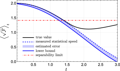
Figure 2: Two-qubit example with local dephasing noise, showing how the time-averaged value of $\sqrt{\mathcal{F}(\eta_{s},\mathcal{V})}$ from $s=0$ to $t$ can be lower-bounded using the speed limit Eq. (12). The initial state $\frac{\ket{00}+\ket{11}}{\sqrt{2}}$ is maximally entangled. In units of $h=1$, we take $\lambda=\gamma=v=0.1$ and $\epsilon\leq 4\lambda^{2}\gamma/h=0.004$. The measured statistical speed is the left-hand side of Eq. (14), taking a measurement in the Bell basis $\{\frac{\ket{00}\pm\ket{11}}{\sqrt{2}},\frac{\ket{01}\pm\ket{10}}{\sqrt{2}}\}$. The estimated error $\frac{2\Delta_{\mathrm{est}}(t)}{vt}$ (indicated by the shaded area) iś subtracted to give the lower bound.

In a weak coupling setting, one can employ the error $\Delta_{\mathrm{est}}(t)$ from Eq. (12) to tighten the threshold value in Eq. (14) to $\sqrt{\mathcal{F}_{*}}+\frac{2\Delta_{\mathrm{est}}(t)}{vt}$. The change in this threshold is roughly $\frac{2\Delta_{\mathrm{est}}(t)}{vt}=\mathcal{O}(\sqrt{\epsilon vt})+\mathcal{O}(\epsilon)$. A simulation of this protocol is shown in Fig. 2 for the two-qubit dephasing model described above. A measurement in the Bell basis $\{\frac{\ket{00}\pm\ket{11}}{\sqrt{2}},\frac{\ket{01}\pm\ket{10}}{\sqrt{2}}\}$ is used for the Bhattacharrya coefficient. For any separable state $\rho_{\mathrm{sep}}$ of two qubits, we have the inequality $\mathcal{F}(\rho_{\mathrm{sep}},\mathcal{V})\leq\mathcal{F}_{*}=2$ [47, 24, 23]. Using the parameters $h=1$ and $\lambda=\gamma=v=0.1$, this threshold is broken by the exact QFI for $t\lessapprox 1.41$, while entanglement is witnessed taking into account the error estimate for $t\lessapprox 1.26$.

Quantum work fluctuations.—Finally, we show the implications of our speed limit for fluctuations in work performed during a sudden quench driving a system out of equilibrium. Consider a system with Hamiltonian $H$ which is initially in thermal equilibrium at inverse temperature $\beta$, in the Gibbs state $\rho_{\mathrm{th}}=\frac{e^{-\beta H}}{\tr e^{-\beta H}}$. At time $0$, the Hamiltonian is quickly changed to $H^{\prime}$, involving fluctuating work $w$ done on the system. The mean and variance of the work are computed from the change in the Hamiltonian $\Delta H=H^{\prime}-H$: $\expectationvalue{w}=\tr[\rho_{\mathrm{th}}\Delta H],\,\mathrm{Var}_{w}=\mathrm{Var}(\rho_{\mathrm{th}},\Delta H)$. If the system is subsequently left to thermalise to the new Gibbs state $\rho_{\mathrm{th}}^{\prime}=\frac{e^{-\beta H^{\prime}}}{\tr e^{-\beta H^{\prime}}}$, then its Helmholtz free energy $F_{H,\beta}$ will decrease. This is defined by $F_{H,\beta}=\tr[\rho_{\mathrm{th}}H]-\beta^{-1}S(\rho_{\mathrm{th}})$, where $S(\rho_{\mathrm{th}})=-\tr[\rho_{\mathrm{th}}\ln\rho_{\mathrm{th}}]$ is the von Neumann entropy [51]. The second law of thermodynamics implies that the change $\Delta F:=F_{H^{\prime},\beta}-F_{H,\beta}\leq\expectationvalue{w}$ – this is equivalent to saying that the dissipated work $W_{\mathrm{diss}}:=\expectationvalue{w}-\Delta F\geq 0$ [51]. $W_{\mathrm{diss}}$ is thus associated with nonequilibrium entropy production.

Figure 3: Driving out of equilibrium: work is performed during a sudden quench $H\to H^{\prime}$. The system moves away from its initial Gibbs state $\rho_{\mathrm{th}}$ to the new one $\rho_{\mathrm{th}}^{\prime}$. The speed limit Eq. (18) bounds the distance between $\rho_{\mathrm{th}}$ and the state $\rho_{t}$ after time $t$ in terms of quantum fluctuations in the work.

In order to study small deviations from equilibrium, we follow the paradigm of, for instance, Refs. [52, 53], in which $\Delta H$ is taken as small. One then finds a fluctuation-dissipation relation [53]

$$\frac{\beta}{2}\mathrm{Var}_{w}=W_{\mathrm{diss}}+Q_{w}.$$ (16)

Here, $Q_{w}\geq 0$ is a quantum correction to the usual relation for classical systems [54, 55], thus Eq. (16) represents a modification of a classical statistical law near equilibrium that takes into account coherent quantum effects. It also implies a barrier to finding coherent protocols that simultaneously minimise work fluctuations and dissipation [53].

The relation Eq. (16) holds for a range of slow driving settings; in our case with a single small quench, $Q_{w}$ is determined by a quantity closely related to the QFI:

$$Q_{w} =\frac{\beta}{2}\bar{I}(\rho_{\mathrm{th}},\Delta H),$$

$$\bar{I}(\rho,A) :=\int_{0}^{1}\differential k\;\frac{1}{2}\tr\left([\rho^{k},A][A,\rho^{1-k}]\right).$$ (17)

The details of this result from Ref. [53] are recalled in Appendix D. Here, $\bar{I}$ belongs to a family of generalised quantum Fisher information quantities [56]. Members of this family are interpreted as measures of quantum coherence (also known as asymmetry in this context): $\bar{I}(\rho,H)$ and $\mathcal{F}(\rho,\mathcal{H})$, among others, quantify the coherence of a state $\rho$ with respect to a Hamiltonian $H$ [26, 57, 20, 37]. Moreover, they can be regarded as quantum contributions to the variance of $H$ [58, 59, 60]. Applied to $\bar{I}$, some of the key properties justifying this interpretation are that $\bar{I}(\rho,H)\leq\mathrm{Var}(\rho,H)$, with equality for pure states, and $\bar{I}(\rho,H)=0$ when $\rho$ commutes with $H$. Therefore, as required of a measure of quantum work fluctuations, $2Q_{w}/\beta=\bar{I}(\rho_{\mathrm{th}},\Delta H)$ vanishes exactly when $[H,\Delta H]=0$.

We now use our speed limit to derive the following bound on how fast the state $\rho_{t}$ can evolve away from the initial Gibbs state (illustrated in Fig. 3).

Result 3.

Quantum work fluctuations are necessary for fast departure from equilibrium. For a system weakly coupled to a thermal environment, at all times $t>0$ following the quench $H\to H^{\prime}$, the distance between the initial Gibbs state $\rho_{\mathrm{th}}$ and the system’s state $\rho_{t}$ is limited by

$$\theta_{B}(\rho_{\mathrm{th}},\rho_{t})\leq t\sqrt{3\bar{I}(\rho_{\mathrm{th}},\Delta H)}+\Delta(t),$$ (18)

where $\Delta(t)$ is the weak coupling error term from Eq. (13).

Proof.

This can be proven by using Result 2 with initial state $\rho_{\mathrm{th}}$, but instead reversing the roles of the perturbed and unperturbed trajectories. So now the unperturbed trajectory involves the Hamiltonian $H^{\prime}$ and its dynamics are generated by $\mathcal{L^{\prime}}$, while the perturbation is $vV=-\Delta H$. Doing it this way around, the QFI appearing on the right-hand side of the speed limit is $\mathcal{F}(\rho_{\mathrm{th}},\Delta\mathcal{H})$, which is constant in time since the perturbed state $\rho_{t}=\rho_{\mathrm{th}}\,\forall\,t\geq 0$ is a steady state under $\mathcal{L}$. The relevant Bures angle is then $\theta_{B}(\rho^{\prime}_{t},\rho_{t})=\theta_{B}(\rho^{\prime}_{t},\rho_{\mathrm{th}})$. We show in Appendix D that the QFI and $\bar{I}$ never differ by more than a constant factor: $4\bar{I}\leq\mathcal{F}\leq 12\bar{I}$. Finally using the the latter inequality, we have $\mathcal{F}(\rho_{\mathrm{th}},\Delta\mathcal{H})\leq 12\bar{I}(\rho_{\mathrm{th}},\Delta H)$. ∎

A fast departure from $\rho_{\mathrm{th}}$ thus requires a large value of quantum work fluctuations as measured by $\bar{I}(\rho_{\mathrm{th}},\Delta H)$ – equivalently, $\rho_{\mathrm{th}}$ must have a high degree of quantum coherence with respect to $\Delta H$.

The physical importance of the correction $\Delta(t)$ is seen in the “classical” case where $[H,\Delta H]=0$ (i.e., the energy levels are changed but not the energy eigenstates). Then $\bar{I}=0$ but the system must deviate from $\rho_{\mathrm{th}}$ in order to reach the new steady state $\rho_{\mathrm{th}}^{\prime}$. From our earlier discussion of the weak coupling error and Eq. (13), by identifying $v$ with $\|\Delta H\|$, we therefore see that the quantum driving regime – i.e., when the term with $\bar{I}$ dominates on the right-hand side of Eq. (18) – corresponds to

$$\frac{\sqrt{\bar{I}(\rho_{\mathrm{th}},\Delta H)}}{\|\Delta H\|}\gg\max\{\sqrt{\epsilon\|\Delta H\|t},\,\epsilon\}.$$ (19)

The left-hand side of this inequality measures the quantum work fluctuations relative to the size of $\Delta H$. In the quantum driving regime, coherent evolution resulting from the change in Hamiltonian happens faster than thermalisation.

Conclusions.—In summary, we have shown that the well-known Mandelstam-Tamm quantum speed limit can be extended to describe the rate of divergence of a perturbed open system from its unperturbed trajectory. We have found that this speed limit holds to a high degree of approximation when a system is weakly coupled to an environment, assuming only a small perturbing Hamiltonian and the standard Born-Markov and secular approximations, and that the error may be bounded with knowledge of the relevant timescales. This results in a practically useful method for experimentally lower-bounding quantum Fisher information, where the error need not be neglected but can be estimated and taken into account. Finally, we used the speed limit to prove that quantum work fluctuations are necessary to have a fast departure from equilibrium in a perturbed system weakly coupled to a thermal environment.

Note that we can derive a similar speed limit along the same lines by instead replacing the Bures angle by the quantity $\tilde{\theta}(\rho,\sigma)=\arccos\tr(\sqrt{\rho}\sqrt{\sigma})$ and the QFI by (four times) the Wigner-Yanase skew information [61], which in the Hamiltonian case reads $I^{\mathrm{WY}}(\rho,\mathcal{V})=-\frac{1}{2}\tr([\sqrt{\rho},V]^{2})$. A first technical question for future work is therefore whether the speed limit can be extended to different distance measures or generalised QFI quantities [56].

In the weak coupling regime, an interesting direction is to find the error term in the case of slow continuous changes to the perturbation, using the theory of adiabatic master equations [62]. This could then generalise Result 3 to take into account continuous driving. A further natural question is whether this has implications for thermodynamic uncertainty relations, which relate current fluctuations to entropy production [63].

Finally, noting that our speed limit holds under the assumption of Markovian dynamics, a violation of the inequality could be used as a witness of non-Markovianity. For this purpose, one would need an independent method to estimate (upper-bound) the QFI, for example via the variance of the perturbing Hamiltonian. This would add to a library of witnesses of non-Markovianity, including those based on the contractivity of QFI over time [38, 52].

Acknowledgments.—We thank Florian Fröwis, George Knee, and Bill Munro for discussions that inspired this work, as well as Stefan Nimmrichter for further input. This project has received funding from the European Union’s Horizon 2020 research and innovation programme under the Marie Skłodowska-Curie grant agreement No. 945422, the DAAD, the Deutsche Forschungsgemeinschaft (DFG, German Research Foundation, project numbers 447948357 and 440958198), the Sino-German Center for Research Promotion (Project M-0294), the ERC (Consolidator Grant 683107/TempoQ), and the German Ministry of Education and Research (Project QuKuK, BMBF Grant No. 16KIS1618K).

Appendix A Weak coupling perturbation

Here, we show the conditions under which the change to a perturbed open system’s dynamics can be approximated as just containing the perturbing Hamiltonian $vV$, and estimate the size of the error. Recall the relevant timescales: $\tau_{S}\sim h^{-1}$ for the system Hamiltonian, $\tau_{V}\sim v^{-1}$ for the perturbation, $\tau_{R}\sim\lambda^{-2}\gamma^{-1}$ for the system relaxation, and $\tau_{B}$ for the bath correlation decay. In terms of these, the assumptions being used are:

1. Born-Markov approximation: $\tau_{B}\ll\tau_{R}$,

2. rotating wave approximation (RWA): $\tau_{S}\ll\tau_{R}$,

3. small perturbation relative to bath: $\tau_{B}\ll\tau_{V}$,

4. small perturbation relative to system: $\tau_{S}\ll\tau_{V}$.

The need for assumption (iii) is not obvious but will become apparent later – it is needed essentially so we can approximate the bath correlation function as flat in the frequency domain. Firstly, we expand the perturbed dissipator $\mathcal{D}^{\prime}$ and Lamb shift $H^{\prime}_{\mathrm{LS}}$ to first order in $v$ using standard perturbation theory [64]. Note that we assume both $H=\sum_{n}E_{n}\outerproduct{n}{n}$ and $H^{\prime}=\sum_{n}E^{\prime}_{n}\outerproduct{n^{\prime}}{n^{\prime}}$ to be non-degenerate. To lowest order, the perturbed energy eigenvalues and eigenvectors are $E^{\prime}_{n}=E_{n}+vE_{n}^{(1)}+\mathcal{O}(v^{2})$, $\ket{n^{\prime}}=\ket{n}+v\ket{n^{(1)}}+\mathcal{O}(v^{2})$, with

$$E^{(1)}_{n} =\matrixelement{n}{V}{n},$$

$$\ket*{n^{(1)}} =\sum_{m\neq n}\frac{\matrixelement{m}{V}{n}}{E_{n}-E_{m}}\ket{m}=:\sum_{m\neq n}C_{nm}\ket{m}.$$ (20)

The perturbed Bohr frequencies are of the form $\omega^{\prime}\approx\omega+\delta\omega$ with $\delta\omega=\mathcal{O}(v)$. It is possible for some $\omega$ to be degenerate, meaning that several transitions may have the same gap (for example, with the energies $\{-1,0,1\}$). We initially assume that the pattern of Bohr frequency degeneracies is unchanged under the perturbation, showing below how to handle a breaking of degeneracy. Recall that the RWA neglects terms in the master equation where $A_{\alpha}(\omega_{1})$ and $A_{\beta}^{\dagger}(\omega_{2})$ occur with $\absolutevalue{\omega_{1}-\omega_{2}}\gg\tau_{R}^{-1}$ [46]. On the other hand, if $\absolutevalue{\omega_{1}-\omega_{2}}\ll\tau_{R}^{-1}$, then we should treat these frequencies as effectively degenerate so that the RWA does not remove such off-diagonal terms, and we can include $A_{\alpha}(\omega_{1})$ and $A_{\alpha}(\omega_{2})$ in the same frequency component of $A_{\alpha}$.

Supposing that the perturbed frequencies $\omega^{\prime}$ have the same pattern of degeneracies as the $\omega$, the perturbed jump operators are

$$A^{\prime}_{\alpha}(\omega^{\prime}) =\sum_{m,n:\>E^{\prime}_{m}-E^{\prime}_{n}\approx\omega^{\prime}}\Pi^{\prime}_{m}A_{\alpha}\Pi^{\prime}_{n}$$

$$=\sum_{m,n:\>E_{m}-E_{n}\approx\omega}\Pi^{\prime}_{m}A_{\alpha}\Pi^{\prime}_{n}$$

$$=\sum_{m,n:\;E_{m}-E_{n}\approx\omega}\Pi_{m}A_{\alpha}\Pi_{n}+v\left(Q_{m}A_{\alpha}\Pi_{n}+\Pi_{m}A_{\alpha}Q_{n}\right)+\mathcal{O}(v^{2})$$

$$=:A_{\alpha}(\omega)+vA^{(1)}_{\alpha}(\omega)+\mathcal{O}(v^{2}),$$ (21)

where the $\approx$ sign is shorthand for equality up to an error much less than $\tau_{R}^{-1}$, i.e., $\absolutevalue{E_{m}-E_{n}-\omega}\ll\tau_{R}^{-1}$, and

$$\Pi^{\prime}_{n} =\Pi_{n}+vQ_{n}+\mathcal{O}(v^{2}),$$

$$Q_{n} :=\sum_{m\neq n}C_{nm}\outerproduct{m}{n}+C_{nm}^{*}\outerproduct{n}{m}.$$ (22)

For the bath correlation coefficients, we write $\gamma_{\alpha\beta}(\omega^{\prime})=\gamma_{\alpha\beta}(\omega)+\delta\omega\partial_{\omega}\gamma_{\alpha\beta}(\omega)+\mathcal{O}(v^{2})$ and similarly for $S_{\alpha\beta}(\omega^{\prime})$. Inserting these into the expressions Eq. (Quantum speed limit for perturbed open systems) to determine the perturbed Lamb shift and dissipator, we have the first order terms

$$vH^{(1)}_{\mathrm{LS}} =\lambda^{2}\sum_{\omega}\sum_{\alpha,\beta}vS_{\alpha\beta}(\omega)\left[{A_{\alpha}^{(1)}}^{\dagger}A_{\beta}(\omega)+A_{\alpha}^{\dagger}(\omega)A_{\beta}^{(1)}(\omega)\right]+\delta\omega\partial_{\omega}S_{\alpha\beta}(\omega)A_{\alpha}^{\dagger}(\omega)A_{\beta}(\omega),$$

$$v\mathcal{D}^{(1)}(\rho) =\lambda^{2}\sum_{\omega}\sum_{\alpha,\beta}v\gamma_{\alpha\beta}(\omega)\left[A_{\beta}^{(1)}(\omega)\rho A_{\alpha}^{\dagger}(\omega)+A_{\beta}(\omega)\rho{A_{\alpha}^{(1)}}^{\dagger}(\omega)-\frac{1}{2}\left\{{A_{\alpha}^{(1)}}^{\dagger}(\omega)A_{\beta}(\omega)+A_{\alpha}^{\dagger}(\omega)A_{\beta}^{(1)}(\omega),\rho\right\}\right]$$

$$\quad+\delta\omega\partial_{\omega}\gamma_{\alpha\beta}(\omega)\left[A_{\beta}(\omega)\rho A_{\alpha}^{\dagger}(\omega)-\frac{1}{2}\left\{A_{\alpha}^{\dagger}(\omega)A_{\beta}(\omega),\rho\right\}\right].$$ (23)

To analyse the size of these terms, we first estimate $\lambda^{2}\absolutevalue{\gamma_{\alpha\beta}(\omega)}\sim\tau_{R}^{-1}$ for all $\omega$ of interest. The first derivative can be found by observing that $\Gamma_{\alpha\beta}(\omega)=\int_{0}^{\infty}\differential s\;e^{i\omega s}\expectationvalue{B_{\alpha}^{\dagger}(s)B_{\beta}(0)}$ implies

$$\absolutevalue{\partial_{\omega}\Gamma_{\alpha\beta}(\omega)} =\absolutevalue{\int_{0}^{\infty}\differential s\;se^{i\omega s}\expectationvalue{B_{\alpha}^{\dagger}(s)B_{\beta}(0)}}$$

$$\sim\tau_{B}\absolutevalue{\Gamma_{\alpha\beta}(\omega)},$$ (24)

given that $\tau_{B}$ is the characteristic decay timescale of the correlation function. Therefore, we can estimate $\lambda^{2}\absolutevalue{\partial_{\omega}\gamma_{\alpha\beta}(\omega)}\sim\tau_{B}\tau_{R}^{-1}$, and similarly for $S_{\alpha\beta}(\omega)$. From the perturbation theory expressions above and the fact that $A_{\alpha}(\omega)=\mathcal{O}(1)$, we further have $A_{\alpha}^{(1)}(\omega)\sim h^{-1}\sim\tau_{S}$. Hence, we see that

$$v\mathcal{H}_{\mathrm{LS}}^{(1)}(\rho)+v\mathcal{D}^{(1)}(\rho) =\mathcal{O}\left(\frac{\tau_{S}}{\tau_{V}\tau_{R}}\right)+\mathcal{O}\left(\frac{\tau_{B}}{\tau_{V}\tau_{R}}\right),$$ (25)

We want to ensure that this term is negligible compared with the other terms in the master equation. It is small compared with $v$ as long as $\tau_{S}\ll\tau_{R}$ and $\tau_{B}\ll\tau_{R}$ – exactly the RWA and Born-Markov conditions, assumptions (ii) and (i) above. Furthermore, it is small compared with $\mathcal{D}$ and $H_{\mathrm{LS}}$ when $\tau_{S}\ll\tau_{V}$ and $\tau_{B}\ll\tau_{V}$, corresponding to the small perturbation assumptions (iv) and (iii).

Finally, we comment on what happens when a degeneracy in the Bohr frequencies is broken by the perturbation. (The simplest example is a three-level system with energies $E_{0}=0,\,E_{1}=\Delta$ and $E_{2}=2\Delta$, with a perturbation shifting the middle level $E_{1}$.) Suppose that $\absolutevalue{\omega_{1}-\omega_{2}}\ll\tau_{R}^{-1}$ but $\absolutevalue{\omega^{\prime}_{1}-\omega^{\prime}_{2}}\gg\tau_{R}^{-1}$. This means the RWA now gets applied to remove the relevant off-diagonal term in the perturbed master equation. Then the error term contains a part of order $\tau_{R}^{-1}$ – of the same magnitude as $\mathcal{D}$ and thus non-negligible. In order to prevent this from happening, in such a situation we therefore need the additional condition $\tau_{R}\ll\tau_{V}$ – i.e., the perturbation must be weaker than the decoherence term. This is stricter than the small perturbation conditions (iii) and (iv) assumed above.

Appendix B Error bounds for weak coupling

Here, we prove Result 2. The triangle inequality for $\theta_{B}$ and an application of Result 1 implies

$$\theta_{B}(\rho_{t},\eta_{t}) \leq\theta_{B}(\rho_{t},\sigma_{t})+\theta_{B}(\sigma_{t},\eta_{t})$$

$$\leq\frac{1}{2}\int_{0}^{t}\differential s\;v\sqrt{\mathcal{F}(\sigma_{s},\mathcal{V})}+\theta_{B}(\sigma_{t},\eta_{t})$$

$$\leq\frac{1}{2}\int_{0}^{t}\differential s\;v\sqrt{\mathcal{F}(\eta_{s},\mathcal{V})}+\Delta_{1}(t)+\Delta_{2}(t),$$ (26)

where the error terms are

$$\Delta_{1}(t) :=\frac{1}{2}\absolutevalue{\int_{0}^{t}\differential s\;v\sqrt{\mathcal{F}(\sigma_{s},\mathcal{V})}-\int_{0}^{t}\differential s\;v\sqrt{\mathcal{F}(\eta_{s},\mathcal{V})}},$$

$$\Delta_{2}(t) :=\theta_{B}(\sigma_{t},\eta_{t}).$$ (27)

In order to bound these errors, we start by showing that $\Delta_{1}$ can be related to $\Delta_{2}$. Firstly, using triangle inequality and then the fact that $(\sqrt{x}-\sqrt{y})^{2}=x+y-2\sqrt{xy}\leq x+y-2\min\{x,y\}=\absolutevalue{x-y}$,

$$\Delta_{1}(t) \leq\frac{v}{2}\int_{0}^{t}\differential s\;\absolutevalue{\sqrt{\mathcal{F}(\sigma_{s},\mathcal{V})}-\sqrt{\mathcal{F}(\eta_{s},\mathcal{V})}}$$

$$\leq\frac{v}{2}\int_{0}^{t}\differential s\;\sqrt{\absolutevalue{\mathcal{F}(\sigma_{s},\mathcal{V})-\mathcal{F}(\eta_{s},\mathcal{V})}}.$$ (28)

Now we use the QFI continuity result Eq. (A6) from Ref. [40]:

$$\absolutevalue{\mathcal{F}(\sigma,\mathcal{V})-\mathcal{F}(\eta,\mathcal{V})}\leq 32D_{B}(\sigma,\eta)\|V\|^{2},$$ (29)

in terms of the Bures distance $D_{B}=\sqrt{2(1-F)}$ which satisfies $D_{B}\leq\theta_{B}$ (where $F$ is the Uhlmann. Inserting this into Eq. (B) gives

$$\Delta_{1}(t) \leq 2\sqrt{2}v\|V\|\int_{0}^{t}\differential s\;\sqrt{\Delta_{2}(s)}.$$ (30)

Now we bound $\Delta_{2}$ using another application of the speed limit in Result 1, now comparing $\sigma_{s}$ and $\eta_{s}$ under the error term $\mathcal{H}_{\mathrm{LS}}^{(1)}+\mathcal{D}^{(1)}$. To lowest order in $v$,

$$\Delta_{2}(t) \leq\frac{v}{2}\int_{0}^{t}\differential s\;\sqrt{\mathcal{F}(\eta_{s},\mathcal{H}_{\mathrm{LS}}^{(1)}+\mathcal{D}^{(1)})}.$$ (31)

The size of the integrand is bounded using Lemma 1 below, giving

$$\Delta_{2}(t) \leq vt\,\max_{\psi}\|\mathcal{H}^{(1)}_{\mathrm{LS}}(\psi)+\mathcal{D}^{(1)}(\psi)\|$$

$$=:vt\epsilon.$$ (32)

The right-hand side of Eq. (B) measures the size of the generator $\mathcal{H}_{\mathrm{LS}}^{(1)}+\mathcal{D}^{(1)}$ in terms of its greatest effect on any pure state. In specific examples (see Appendix C) this norm can be calculated explicitly; from Eq. (25), we can generally estimate

$$\epsilon=\mathcal{O}\left(\frac{\tau_{S}}{\tau_{R}}\right)+\mathcal{O}\left(\frac{\tau_{B}}{\tau_{R}}\right).$$ (33)

Inserting into Eq. (30), we have

$$\Delta_{1}(t) \leq 2\sqrt{2}v\|V\|\int_{0}^{t}\differential s\;\sqrt{v\epsilon s}$$

$$=\frac{4\sqrt{2}}{3}\|V\|\epsilon^{\frac{1}{2}}(vt)^{\frac{3}{2}}.$$ (34)

The validity and tightness of these estimates are shown in Fig. 4 for the two-qubit model described in Appendix C.

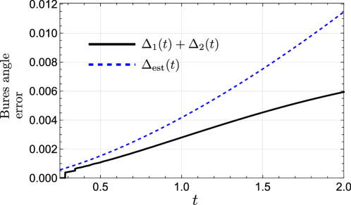
Figure 4: Demonstration of error bound for the two-qubit example, taking the same parameters as in Fig. 2. The error being shown is that on the right-hand side of the weak coupling speed limit Eq. (12): both the sum of the terms $\Delta_{1}(t)+\Delta_{2}(t)$ from Eq. (B) (which in this case is dominated by $\Delta_{2}$) and the upper bound estimate $\Delta_{\mathrm{est}}(t)$ from Eqs. (30), (B).

Lemma 1.

For any state $\rho$ and generator $\mathcal{L}$, we have $\mathcal{F}(\rho,\mathcal{L})\leq 4\max_{\psi}\|\mathcal{L}(\psi)\|^{2}$, with the maximisation being over pure states $\psi$.

Proof.

Convexity of QFI says that, for any pure state ensemble decomposition $\rho=\sum_{i}p_{i}\outerproduct{\psi_{i}}{\psi_{i}}$, $\mathcal{F}(\rho,\mathcal{L})\leq\sum_{i}p_{i}\mathcal{F}(\psi_{i},\mathcal{L})$. Therefore the maximal QFI can always be achieved with some pure state $\psi$. We employ the expression Eq. (2) with an orthogonal basis $\{\ket{i}\}_{i}$ chosen such that $\ket{0}=\ket{\psi}$, getting

$$\mathcal{F}(\psi,\mathcal{L}) =2\sum_{i,j}\frac{\absolutevalue{\matrixelement{i}{\mathcal{L}(\psi)}{j}}^{2}}{\lambda_{i}+\lambda_{j}}$$

$$=2\left[\frac{\absolutevalue{\expectationvalue{\mathcal{L}(\psi)}{\psi}}^{2}}{2}+2\sum_{i>0}\absolutevalue{\matrixelement{i}{\mathcal{L}(\psi)}{\psi}}^{2}\right]$$

$$=\expectationvalue{\mathcal{L}(\psi)}{\psi}^{2}+4\sum_{i>0}\matrixelement{\psi}{\mathcal{L}(\psi)}{i}\matrixelement{i}{\mathcal{L}(\psi)}{\psi}$$

$$=\expectationvalue{\mathcal{L}(\psi)}{\psi}^{2}+4\bra{\psi}\mathcal{L}(\psi)\left(\mathbbm{1}-\outerproduct{\psi}{\psi}\right)\mathcal{L}(\psi)\ket{\psi}$$

$$=4\expectationvalue{\mathcal{L}(\psi)^{2}}{\psi}-3\expectationvalue{\mathcal{L}(\psi)}{\psi}^{2}$$

$$\leq 4\expectationvalue{\mathcal{L}(\psi)^{2}}{\psi}.$$ (35)

Finally, we note that $\expectationvalue{\mathcal{L}(\psi)^{2}}{\psi}\leq\|\mathcal{L}(\psi)^{2}\|\leq\|\mathcal{L}(\psi)\|^{2}$. ∎

Appendix C Two-qubit dephasing model

Our example is a two-qubit system in which each qubit dephases by interacting independently with a bath of harmonic oscillators – see, for example, Ref. [42]. First consider a single qubit with Hamiltonian $H=\frac{h}{2}\sigma_{z}$ and perturbed with $V=\frac{1}{2}\sigma_{x}$, and a bath whose Hamiltonian is $H_{B}=\sum_{k}\omega_{k}b_{k}^{\dagger}b_{k}$, where $b_{k}$ is the bosonic annihilation operator for mode $k$. The interaction is $H_{I}=\lambda\sigma_{z}\otimes\sum_{k}g_{k}(b_{k}+b_{k}^{\dagger})$, with $g_{k}$ being dimensionless coupling coefficients. We take the continuum limit with an Ohmic bath, replacing $g_{k}^{2}$ by a spectral density function $J(\omega)=\eta\omega e^{-\omega/\omega_{c}}$. Here, $\eta$ is a constant with dimensions of time squared and $\omega_{c}$ is a cut-off frequency that we take to be large compared with all other relevant frequency scales. Given that the bath is in a thermal state at inverse temperature $\beta$, one can derive [42]

$$\gamma(\omega)=\frac{2\pi\eta e^{-\absolutevalue{\omega}/\omega_{c}}}{1-e^{-\beta\omega}}.$$ (36)

Since there is a single jump operator in the master equation, $A=A(0)=\sigma_{z}$, from the results in Appendix A, we find $A^{(1)}(0)=\sigma_{x}$ and thus

$$H_{\mathrm{LS}}^{(1)} =0,$$

$$\mathcal{D}^{(1)}(\rho) =\frac{\lambda^{2}\gamma(0)}{h}\left(\sigma_{z}\rho\sigma_{x}+\sigma_{x}\rho\sigma_{z}\right).$$ (37)

Then $\gamma(0)=2\pi\eta/\beta$ and $\tau_{B}\sim\beta$. In this case, note that the derivative $\partial_{\omega}\gamma(\omega)$ does not appear. However, for large $\omega_{c}$ one finds $\lim_{\omega\to 0^{+}}\partial_{\omega}\gamma(\omega)\approx\lim_{\omega\to 0^{-}}\partial_{\omega}\gamma(\omega)\approx\pi\eta\sim\gamma(0)\tau_{B}$ – consistent with the claim in Eq. (A). The error terms are easily bounded using

$$\|\sigma_{z}\psi\sigma_{x}+\sigma_{x}\psi\sigma_{z}\| \leq 2\|\sigma_{z}\psi\sigma_{x}\|$$

$$\leq 2\|\sigma_{z}\|\|\psi\|\|\sigma_{x}\|$$

$$=2.$$ (38)

The single-qubit error parameter $\epsilon_{1}$ is therefore bounded by $\epsilon_{1}\leq 2\lambda^{2}\gamma(0)/h$.

For the two-qubit system, we take the same independent dynamics on each qubit (so that $H=\frac{h}{2}(\sigma_{z}\otimes\mathbbm{1}+\mathbbm{1}\otimes\sigma_{z})$ and so on). This gives $\epsilon=\max_{\psi}\|[\mathcal{D}^{(1)}\otimes\mathbbm{1}+\mathbbm{1}\otimes\mathcal{D}^{(1)}](\psi)\|\leq 2\epsilon_{1}\leq 4\lambda^{2}\gamma(0)/h$. Note that an extension of this model to $N$ qubits would have an error term scaling with $N$; a similar analysis could also be performed for a collective decoherence model where all qubits couple to the same bath [65].

Appendix D Details of work fluctuations

Here, we first recall the derivation in Ref. [53] of Eq. (16). It starts from writing the dissipated work in terms of relative entropy as $\beta W_{\mathrm{diss}}=S(\rho_{\mathrm{th}}||\rho_{\mathrm{th}}^{\prime})=\tr[(\rho_{\mathrm{th}}-\rho_{\mathrm{th}}^{\prime})\ln\rho_{\mathrm{th}}^{\prime}]$. For small $\Delta H$, this can be approximated to lowest order as

$$W_{\mathrm{diss}}\approx\frac{\beta}{2}\mathrm{Var}^{\mathrm{K}}(\rho_{\mathrm{th}},\Delta H),$$ (39)

where $\mathrm{Var}^{\mathrm{K}}$ is the so-called Kubo-Mori generalised variance [56]. This can be expressed using a superoperator $\mathbb{J}_{\rho}$ which depends on a given state $\rho$:

$$\mathbb{J}_{\rho}(A)=\sum_{i,j}\frac{\lambda_{i}-\lambda_{j}}{\ln\lambda_{i}-\ln\lambda_{j}}\matrixelement{\psi_{i}}{A}{\psi_{j}}\outerproduct{\psi_{i}}{\psi_{j}},$$ (40)

where $\lambda_{i}$ and $\ket{\psi_{i}}$ are the eigenvalues and eigenvectors of $\rho$. Then we have $\mathrm{Var}^{\mathrm{K}}(\rho,A):=\tr\left[\bar{A}\mathbb{J}_{\rho}(\bar{A})\right]$, with $\bar{A}:=A-\tr[\rho A]\mathbbm{1}$. The crucial property is the splitting of the variance of $\Delta H$ into two terms: $\mathrm{Var}(\rho_{\mathrm{th}},\Delta H)=\mathrm{Var}^{\mathrm{K}}(\rho_{\mathrm{th}},\Delta H)+\bar{I}(\rho_{\mathrm{th}},\Delta H)$, interpreted as classical and quantum components respectively (see also Ref. [60]).

We also require the connection between $\bar{I}$ and the QFI proved in Lemma 2 below. This makes use of the theory of generalised QFI quantities – see Ref. [56] for details. Every generalised “skew information” $I^{f}$ corresponds to a function $f\colon\mathbb{R}^{+}\to\mathbb{R}^{+}$ fulfilling the conditions $f(1)=1$, $xf(x^{-1})=f(x)$, and being a matrix monotone. If $f(0)\neq 0$, it is possible to normalise $I^{f}$ to be “metric-adjusted” [66], such that $I^{f}(\outerproduct{\psi}{\psi},H)=\mathrm{Var}(\outerproduct{\psi}{\psi},H)$ for all pure states. Explicitly, we have

$$I^{f}(\rho,H) =\frac{f(0)}{2}\sum_{i,j}\frac{(\lambda_{i}-\lambda_{j})^{2}}{\lambda_{j}f(\lambda_{i}/\lambda_{j})}\absolutevalue{\matrixelement{i}{H}{j}}^{2}.$$ (41)

The case $f(x)=\frac{x+1}{2}$ is often denoted by $I^{\mathrm{SLD}}$ (standing for “symmetric logarithmic derivative”) and recovers the standard QFI under evolution generated by $H$: $4I^{\mathrm{SLD}}(\rho,H)=\mathcal{F}(\rho,\mathcal{H})$.

Lemma 2.

For all states $\rho$ and observables $H$,

$$4\bar{I}(\rho,H)\leq\mathcal{F}(\rho,\mathcal{H})\leq 12\bar{I}(\rho,H).$$ (42)

Proof.

We start from the definition $I^{(k)}(\rho,H):=\frac{1}{2}\tr\left([\rho^{k},H][H,\rho^{1-k}]\right)$, such that $\bar{I}=\int_{0}^{1}\differential k\;I^{(k)}$. We can rewrite $I^{(k)}$ in terms of the matrix elements $H_{ij}:=\matrixelement{\psi_{i}}{H}{\psi_{j}}$ in the eigenbasis of $\rho=\sum_{i}\lambda_{i}\outerproduct{\psi_{i}}{\psi_{i}}$:

$$I^{(k)}(\rho,H) =\tr\left(\rho H^{2}-\rho^{k}H\rho^{1-k}H\right)$$

$$=\sum_{i,j}(\lambda_{i}-\lambda_{i}^{k}\lambda_{j}^{1-k})H_{ij}H_{ji}$$

$$=\sum_{i,j}\frac{1}{2}(\lambda_{i}+\lambda_{j}-\lambda_{i}^{k}\lambda_{j}^{1-k}-\lambda_{i}^{1-k}\lambda_{j}^{k})\absolutevalue{H_{ij}}^{2}$$

$$=\sum_{i,j}\frac{1}{2}(\lambda_{i}^{k}-\lambda_{j}^{k})(\lambda_{i}^{1-k}-\lambda_{j}^{1-k})\absolutevalue{H_{ij}}^{2}$$

$$=\frac{f^{(k)}(0)}{2}\sum_{i,j}\frac{(\lambda_{i}-\lambda_{j})^{2}}{\lambda_{j}f^{(k)}(\lambda_{i}/\lambda_{j})}\absolutevalue{H_{ij}}^{2},$$ (43)

where $f^{(k)}$ is the matrix monotone function corresponding to $I^{(k)}$. We must therefore have

$$f^{(k)}(x)\propto\frac{(x-1)^{2}}{(x^{k}-1)(x^{1-k}-1)}.$$ (44)

In order to be normalised in the standard way, we require $f^{(k)}(1)=1$; taking the limit $x\to 1$ in the above shows that

$$f^{(k)}(x)=\frac{k(1-k)(x-1)^{2}}{(x^{k}-1)(x^{1-k}-1)}$$ (45)

and $f^{(k)}(0)=k(1-k)$. For all metric-adjusted skew informations we have the inequality $I^{f}\leq I^{\mathrm{SLD}}\leq\frac{I^{f}}{2f(0)}$ [59]. It is immediate from its definition that $I^{(k)}$ is metric-adjusted. Thus, the lower bound on $\mathcal{F}=4I^{\mathrm{SLD}}$ is immediate, and we also have

$$I^{(k)}(\rho,H) \geq 2f^{(k)}(0)I^{\mathrm{SLD}}(\rho,H)$$

$$=\frac{f^{(k)}(0)}{2}\mathcal{F}(\rho,\mathcal{H}),$$

$$=\frac{k(1-k)}{2}\mathcal{F}(\rho,\mathcal{H}).$$ (46)

Finally,

$$\bar{I}(\rho,H) \geq\int_{0}^{1}\differential k\;\frac{k(1-k)}{2}\mathcal{F}(\rho,\mathcal{H})$$

$$=\frac{1}{12}\mathcal{F}(\rho,\mathcal{H}).$$ (47)

∎

References

Mandelstam and Tamm [1945]L. Mandelstam and I. Tamm, The uncertainty relation
between energy and time in non-relativistic quantum mechanics, Journal of Physics (USSR) IX, 249 (1945).
del Campo et al. [2013]A. del
Campo, I. L. Egusquiza,
M. B. Plenio, and S. F. Huelga, Quantum Speed Limits in Open System Dynamics, Physical Review Letters 110, 050403 (2013).
Pires et al. [2016]D. P. Pires, M. Cianciaruso,
L. C. Céleri,
G. Adesso, and D. O. Soares-Pinto, Generalized Geometric Quantum Speed Limits, Physical Review X 6, 021031 (2016).
Braunstein and Caves [1994]S. L. Braunstein and C. M. Caves, Statistical distance and
the geometry of quantum states, Physical Review Letters 72, 3439 (1994).
Mukherjee et al. [2016]V. Mukherjee, W. Niedenzu,
A. G. Kofman, and G. Kurizki, Speed and efficiency limits of multilevel
incoherent heat engines, Physical Review E 94, 062109 (2016), 1607.08452 .
Binder et al. [2015]F. C. Binder, S. Vinjanampathy, K. Modi, and J. Goold, Quantacell: powerful charging of
quantum batteries, New Journal of Physics 17, 075015 (2015).
Campaioli et al. [2017]F. Campaioli, F. A. Pollock, F. C. Binder,
L. Céleri, J. Goold, S. Vinjanampathy, and K. Modi, Enhancing the Charging Power of Quantum Batteries, Physical Review Letters 118, 150601 (2017).
Gessner and Smerzi [2018]M. Gessner and A. Smerzi, Statistical speed of
quantum states: Generalized quantum Fisher information and Schatten speed, Physical Review A 97, 022109 (2018).
Zhang et al. [2017]C. Zhang, B. Yadin,
Z.-B. Hou, H. Cao, B.-H. Liu, Y.-F. Huang, R. Maity, V. Vedral, C.-F. Li, G.-C. Guo, and D. Girolami, Detecting
metrologically useful asymmetry and entanglement by a few local
measurements, Physical Review A 96, 042327 (2017).
Hyllus et al. [2012]P. Hyllus, W. Laskowski,
R. Krischek, C. Schwemmer, W. Wieczorek, H. Weinfurter, L. Pezzé, and A. Smerzi, Fisher information and multiparticle entanglement, Physical Review A 85, 022321 (2012).
Morris et al. [2020]B. Morris, B. Yadin,
M. Fadel, T. Zibold, P. Treutlein, and G. Adesso, Entanglement between Identical Particles Is a Useful and Consistent
Resource, Physical Review X 10, 41012 (2020).
Yadin and Vedral [2016]B. Yadin and V. Vedral, General framework for quantum
macroscopicity in terms of coherence, Physical Review A 93, 022122 (2016).
Fröwis et al. [2018]F. Fröwis, P. Sekatski, W. Dür,
N. Gisin, and N. Sangouard, Macroscopic quantum states: Measures, fragility, and
implementations, Reviews of Modern Physics 90, 025004 (2018).
Yadin et al. [2018]B. Yadin, F. C. Binder,
J. Thompson, V. Narasimhachar, M. Gu, and M. S. Kim, Operational Resource Theory of Continuous-Variable
Nonclassicality, Physical Review X 8, 041038 (2018).
Kwon et al. [2019]H. Kwon, K. C. Tan,
T. Volkoff, and H. Jeong, Nonclassicality as a Quantifiable Resource for Quantum
Metrology, Physical Review Letters 122, 040503 (2019).
Strobel et al. [2014]H. Strobel, W. Muessel,
D. Linnemann, T. Zibold, D. B. Hume, L. Pezze, A. Smerzi, and M. K. Oberthaler, Fisher
information and entanglement of non-Gaussian spin states, Science 345, 424 (2014).
Nielsen and Chuang [2010]M. A. Nielsen and I. L. Chuang, Quantum Computation and
Quantum Information (Cambridge University Press, Cambridge, 2010) Chap. 9.
Augusiak et al. [2016]R. Augusiak, J. Kołodyński, A. Streltsov, M. N. Bera,
A. Acín, and M. Lewenstein, Asymptotic role of entanglement in quantum
metrology, Physical Review A 94, 012339 (2016).
Taddei et al. [2013]M. M. Taddei, B. M. Escher,
L. Davidovich, and R. L. de Matos Filho, Quantum Speed Limit for Physical
Processes, Physical Review Letters 110, 050402 (2013).
Ciccarello et al. [2022]F. Ciccarello, S. Lorenzo,
V. Giovannetti, and G. M. Palma, Quantum collision models: Open system dynamics
from repeated interactions, Physics Reports 954, 1 (2022).
Rivas et al. [2010]Á. Rivas, A. D. K
Plato, S. F. Huelga, and M. B Plenio, Markovian master equations: a
critical study, New Journal of Physics 12, 113032 (2010).
Yadin et al. [2021]B. Yadin, M. Fadel, and M. Gessner, Metrological complementarity reveals the
Einstein-Podolsky-Rosen paradox, Nature Communications 12, 2410 (2021).
Bhattacharyya [1943]A. Bhattacharyya, On a measure of
divergence between two statistical populations defined by their probability
distribution, Bulletin of the Calcutta Mathematical Society 35, 99 (1943).
Scandi and Perarnau-Llobet [2019]M. Scandi and M. Perarnau-Llobet, Thermodynamic
length in open quantum systems, Quantum 3, 197 (2019).
Miller et al. [2019]H. J. Miller, M. Scandi,
J. Anders, and M. Perarnau-Llobet, Work Fluctuations in Slow Processes: Quantum
Signatures and Optimal Control, Physical Review Letters 123, 230603 (2019).
Frérot and Roscilde [2016]I. Frérot and T. Roscilde, Quantum variance: A
measure of quantum coherence and quantum correlations for many-body
systems, Physical Review B 94, 075121 (2016).
Horowitz and Gingrich [2020]J. M. Horowitz and T. R. Gingrich, Thermodynamic
uncertainty relations constrain non-equilibrium fluctuations, Nature Physics 16, 15 (2020).
Sakurai and Commins [1995]J. J. Sakurai and E. D. Commins, Modern quantum mechanics,
revised edition (1995).
Kempe et al. [2001]J. Kempe, D. Bacon,
D. A. Lidar, and K. B. Whaley, Theory of decoherence-free fault-tolerant
universal quantum computation, Physical Review A 63, 042307 (2001).