Deterministic Objective Bayesian Analysis for Spatial Models

Abstract

Berger et al. (2001) and Ren et al. (2012) derived noninformative priors for Gaussian process models of spatially correlated data using the reference prior approach (Berger, Bernardo, 1991). The priors have good statistical properties and provide a basis for objective Bayesian analysis (Berger, 2006). Using a trust-region algorithm for optimization with exact equations for posterior derivatives and an adaptive sparse grid at Chebyshev nodes, this paper develops deterministic algorithms for fully Bayesian prediction and inference with the priors. Implementations of the algorithms are available at https://github.com/rnburn/bbai.

1 Introduction

Suppose we observe a Gaussian process $Z(\cdot)$ at sample points ${\boldsymbol{s}}_{1},\ldots,{\boldsymbol{s}}_{n}$ where

$$\operatorname{\mathbb{E}}\left\{Z({\boldsymbol{s}})\right\} =\beta_{1}x_{1}({\boldsymbol{s}})+\cdots+\beta_{p}x_{p}({\boldsymbol{s}})$$

$$=\boldsymbol{\beta}^{\prime}\boldsymbol{x}({\boldsymbol{s}});$$

$$\operatorname{cov}\left\{Z({\boldsymbol{s}}),Z(\boldsymbol{\mathrm{u}})\right\} =\sigma^{2}\left\{\operatorname{\psi}_{\ell}(\left\|{\boldsymbol{s}}-\boldsymbol{\mathrm{u}}\right\|)+\eta\right\};$$ (1)

$\boldsymbol{x}(\cdot)$ and $\operatorname{\psi}_{\ell}(\cdot)$ represent the known regressor function and correlation function; and $\boldsymbol{\beta}$, $\sigma^{2}$, $\ell$, and $\eta$ represent the unknown regression coefficients, signal variance, length, and noise-to-signal ratio.

Let $\boldsymbol{\theta}$ denote the unknown parameters $\left(\boldsymbol{\beta},\sigma^{2},\ell,\eta\right)^{\prime}$. To reason about possible values at unobserved points, we’d like to know the distribution $\operatorname{P}\left(Z(\boldsymbol{\mathrm{u}})\mid\boldsymbol{\mathrm{y}},\boldsymbol{\theta}_{\textrm{true}}\right)$ where $\boldsymbol{\mathrm{u}}$ is an unobserved point and $\boldsymbol{\mathrm{y}}$ denotes the observations $\left(Z({\boldsymbol{s}}_{1}),\ldots,Z({\boldsymbol{s}}_{n})\right)^{\prime}$. Of course, different values of $\boldsymbol{\theta}$ could reasonably produce $\boldsymbol{\mathrm{y}}$, so there’s no way we can identify $\boldsymbol{\theta}_{\textrm{true}}$ or construct prediction distributions exactly. We need ways to approximate.

Approach 1: Maximize Likelihood

Suppose the likelihood function, $L(\boldsymbol{\theta};\boldsymbol{\mathrm{y}})\propto\operatorname{P}\left(\boldsymbol{\mathrm{y}}\mid\boldsymbol{\theta}\right)$, is strongly peaked about an optimum, $\boldsymbol{\theta}_{\textrm{ml}}$. Then $\boldsymbol{\theta}_{\textrm{true}}$ should be close to $\boldsymbol{\theta}_{\textrm{ml}}$, and $\operatorname{P}\left(Z(\boldsymbol{\mathrm{u}})\mid\boldsymbol{\mathrm{y}},\boldsymbol{\theta}_{\textrm{ml}}\right)$ should be a reasonable substitute for $\operatorname{P}\left(Z(\boldsymbol{\mathrm{u}})\mid\boldsymbol{\mathrm{y}},\boldsymbol{\theta}_{\textrm{true}}\right)$.

But what happens if a broad range of parameters could reasonably produce $\boldsymbol{\mathrm{y}}$?

Example 1.1.

[source] Consider the data set from Table 1. I randomly sampled the Gaussian process (1) with

$$\sigma^{2}=25,\quad\ell=0.01,\quad\eta=0.1,\;\;\textrm{and}\;\operatorname{\psi}_{\ell}(t)=\exp\left\{-\frac{t^{2}}{2\ell^{2}}\right\}$$ (2)

at 20 evenly spaced points on the interval $[0,1]$. Likelihood has a maximum at

$$\sigma^{2}_{\textrm{ml}}=34.42,\quad\ell_{\textrm{ml}}=0.035,\;\;\eta_{\textrm{ml}}=3.82\times 10^{-6}.$$

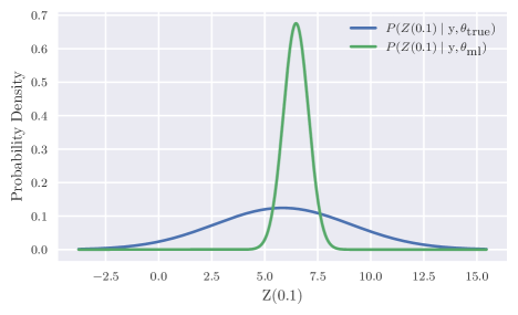
Note how much smaller $\eta_{\textrm{ml}}$ is than its true value. If we try to use $\boldsymbol{\theta}_{\textrm{ml}}$ as a substitute for $\boldsymbol{\theta}_{\textrm{true}}$, we will get bad results as Figure 1 shows. Put

$$g(t)=L(\boldsymbol{\theta}_{\textrm{ml}}(1-t)+\boldsymbol{\theta}_{\textrm{true}}t;\boldsymbol{\mathrm{y}})/L(\boldsymbol{\theta}_{\textrm{ml}};\boldsymbol{\mathrm{y}}).$$

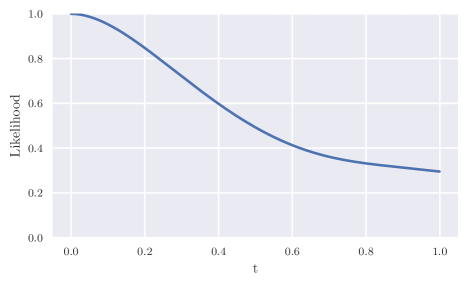
$g(\cdot)$ computes the relative likelihood along a line segment from $\boldsymbol{\theta}_{\textrm{ml}}$ to $\boldsymbol{\theta}_{\textrm{true}}$, and Figure 2 plots $g(t)$ for $0\leq t\leq 1$. Looking at the figure, we can confirm that likelihood is not strongly peaked about an optimum and any value of $\boldsymbol{\theta}$ along the line segment could have reasonably produced $\boldsymbol{\mathrm{y}}$.

$i$	$s$	$y$	$i$	$s$	$y$
1	0.00	6.34	11	0.53	2.25
2	0.05	1.62	12	0.58	4.30
3	0.11	7.38	13	0.63	-4.40
4	0.16	12.22	14	0.68	-2.54
5	0.21	3.03	15	0.74	10.94
6	0.26	-4.58	16	0.79	-2.81
7	0.32	-3.45	17	0.84	-2.82
8	0.37	-4.48	18	0.89	2.53
9	0.42	-8.02	19	0.95	10.01
10	0.47	2.61	20	1.00	1.52

Table 1: Randomly sampled data from Gaussian process (2)

.

Figure 1: Compare Gaussian process prediction distributions $\operatorname{P}\left(Z(0.1)\mid\boldsymbol{\mathrm{y}},\boldsymbol{\theta}_{\textrm{ml}}\right)$ and $\operatorname{P}\left(Z(0.1)\mid\boldsymbol{\mathrm{y}},\boldsymbol{\theta}_{\textrm{true}}\right)$

Figure 2: Relative likelihood for different values of $\boldsymbol{\theta}$ on the line segment from $\boldsymbol{\theta}_{\textrm{ml}}$ to $\boldsymbol{\theta}_{\textrm{true}}$

Approach 2: Integrate over Possible Parameters

We saw in Example 1.1 that using maximum likelihood parameters can lead to poor results when the likelihood function isn’t strongly peaked (Berger et al., 1999). Instead of approximating prediction distributions with only a single value of $\boldsymbol{\theta}$, let’s consider every $\boldsymbol{\theta}$ and weigh by a posterior distribution, $\operatorname{\pi}\left(\boldsymbol{\theta}\mid\boldsymbol{\mathrm{y}}\right)$,

$$\operatorname{P^{\pi}}\left(Z(\boldsymbol{\mathrm{u}})\mid\boldsymbol{\mathrm{y}}\right)=\int\operatorname{P}\left(Z(\boldsymbol{\mathrm{u}})\mid\boldsymbol{\mathrm{y}},\boldsymbol{\theta}\right)\operatorname{\pi}\left(\boldsymbol{\theta}\mid\boldsymbol{\mathrm{y}}\right)d\boldsymbol{\theta}.$$

$\operatorname{\pi}\left(\boldsymbol{\theta}\mid\boldsymbol{\mathrm{y}}\right)$ measures our belief that parameters $\boldsymbol{\theta}$ generated the observations $\boldsymbol{\mathrm{y}}$. To derive $\operatorname{\pi}\left(\boldsymbol{\theta}\mid\boldsymbol{\mathrm{y}}\right)$, we apply Bayes’ theorem: $\operatorname{\pi}\left(\boldsymbol{\theta}\mid\boldsymbol{\mathrm{y}}\right)\propto L(\boldsymbol{\theta};\boldsymbol{\mathrm{y}})\times\operatorname{\pi}\left(\boldsymbol{\theta}\right)$ where $\operatorname{\pi}\left(\boldsymbol{\theta}\right)$ measures our prior belief that the model has parameters $\boldsymbol{\theta}$.

Naturally, this leads to the question: How do we specify $\operatorname{\pi}\left(\boldsymbol{\theta}\right)$ when we know nothing particular about $\boldsymbol{\theta}$? Statisticians have grappled with the problem of specifying so-called noninformative priors ever since Bayes and Laplace first started applying the approach to the binomial model over 200 years ago.

While noninformative priors continue to be debated, fortunately, the modern approach of reference priors gives a general path forward and, particularly, for the case of Gaussian processes works quite well.

Before getting into the details (see §3 and §4 for descriptions of the prior and prediction algorithm), let’s look at how the approach works on the Gaussian process from Example 1.1.

Example 1.2.

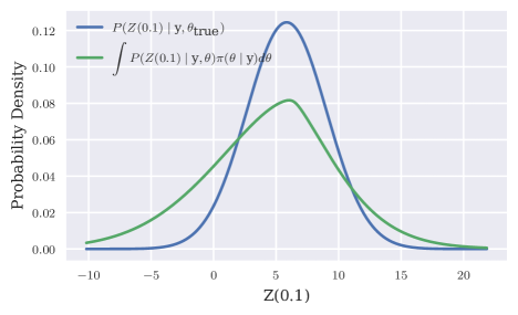
[source] (Example 1.1 continued) In Figure 3, I plot the prediction distribution for the Example 1.1 data set using the Bayesian approach with a reference prior and compare to the true prediction distribution. We can see that the Bayesian approach gives a better approximation to the true prediction distribution than the maximum likelihood approach, Figure 1.

Figure 3: Compare the prediction distribution from the Bayesian approach with reference prior, $\operatorname{P^{\pi}}\left(Z(0.1)\mid\boldsymbol{\mathrm{y}}\right)$, to the true prediction distribution $\operatorname{P}\left(Z(0.1)\mid\boldsymbol{\mathrm{y}},\boldsymbol{\theta}_{\textrm{true}}\right)$.

2 How to Specify Noninformative Priors

The goal of a noninformative prior is to represent “minimal information” so that inference is driven by the data and the model rather than prior knowledge.

Making this goal exact is difficult; and it’s unlikely there will ever be a universal approach to noninformative priors that’s optimal for all situations, as there can be multiple reasonable definitions of “minimal information”. However, frequentist coverage has emerged as one key metric to test whether a candidate noninformative prior is suitable for objective Bayesian analysis. Here’s the basic idea: Let $\Theta_{1}\times\cdots\times\Theta_{k}$ denote the parameter space for the model, pick $\alpha$ to be something like $0.95$, and run Algorithm 1 for different $\tilde{\boldsymbol{\theta}}$ varied across the model’s parameter space. If the prior is good, Algorithm 1 should produce a result close to $\alpha$.

Algorithm 1 Test accuracy of credible sets produced with a prior

1:function coverage-test($\tilde{\boldsymbol{\theta}}$, $j$, $\alpha$)

2:     $cnt$ $\leftarrow$ $0$

3:     $N$ $\leftarrow$ a large number

4:     for $i\leftarrow 1\textrm{ to }N$ do

5:         $\tilde{\boldsymbol{\mathrm{y}}}$ $\leftarrow$ sample from $P(\cdot\mid\tilde{\boldsymbol{\theta}})$

6:         $\tilde{\boldsymbol{\Theta}}$ $\leftarrow$ $\Theta_{1}\times\cdots\times\Theta_{j-1}\times\Theta_{j}\cap(-\infty,\tilde{\theta_{j}}]\times\Theta_{j+1}\times\cdots\times\Theta_{k}$

7:         $t$ $\leftarrow$ $\int_{\tilde{\boldsymbol{\Theta}}}\pi(\boldsymbol{\theta}\mid\tilde{\boldsymbol{\mathrm{y}}})d\boldsymbol{\theta}$

8:         if $\frac{\alpha}{2}<t<1-\frac{\alpha}{2}$ then

9:              $cnt$ $\leftarrow$ $cnt+1$

10:         end if

11:     end for

12:     return $\frac{cnt}{N}$

13:end function

With Algorithm 1 in our toolbox, let’s look at a few approaches for specifying noninformative priors.

Constant Prior

We begin with the simplest approach: Set $\operatorname{\pi}\left(\boldsymbol{\theta}\right)\propto 1$. Immediately, we see one serious disadvantage of this approach: It’s not invariant under reparameterization. If $\varphi(\cdot)$ is some strictly increasing function onto $[a,b]$ with continuous derivative, then

$$\int_{a}^{b}L(\theta;\boldsymbol{\mathrm{y}})d\theta=\int_{\varphi^{-1}(a)}^{\varphi^{-1}(b)}L(\varphi(u);\boldsymbol{\mathrm{y}})\dot{\varphi}(u)du.$$

Thus, different parameterizations with the constant prior lead to different posterior distributions.

Still, let’s try the approach out on some examples.

Example 2.1.

[source] Suppose we observe $n$ normally distributed values, $\boldsymbol{\mathrm{y}}$, with variance $1$ and unknown mean, $\mu$. Then

$$L(\mu;\boldsymbol{\mathrm{y}}) \propto\exp\left\{-\frac{1}{2}\left(\boldsymbol{\mathrm{y}}-\mu\boldsymbol{1}\right)^{\prime}\left(\boldsymbol{\mathrm{y}}-\mu\boldsymbol{1}\right)\right\}$$

$$\propto\exp\left\{-\frac{1}{2}\left(n\mu^{2}-2\mu n\bar{y}\right)\right\}$$

$$\propto\exp\left\{-\frac{n}{2}\left(\mu-\bar{y}\right)^{2}\right\}.$$

Thus,

$$\int_{-\infty}^{t}\operatorname{\pi}\left(\mu\mid\boldsymbol{\mathrm{y}}\right)d\mu=\frac{1}{2}\left[1+\operatorname{erf}\left(\frac{t-\bar{y}}{\sqrt{2/n}}\right)\right].$$

I ran Algorithm 1 for $N={\text{\unboldmath$\mathrm{10{,}000}$}}$, $\alpha=0.95$, and various values of $\mu$ and $n$. Table 2 shows the results.

$n=5$		$n=10$		$n=15$		$n=20$
$\sigma^{2}$	coverage	$\sigma^{2}$	coverage	$\sigma^{2}$	coverage	$\sigma^{2}$	coverage
0.1	0.9502	0.1	0.9486	0.1	0.9508	0.1	0.9493
0.5	0.9519	0.5	0.9478	0.5	0.9492	0.5	0.9488
1.0	0.9516	1.0	0.9495	1.0	0.9517	1.0	0.9494
2.0	0.9514	2.0	0.9521	2.0	0.9539	2.0	0.9489
5.0	0.9489	5.0	0.9455	5.0	0.9558	5.0	0.9488

Table 2: Frequentist coverages for the mean of a normal distribution with known variance and constant prior.

Example 2.2.

[source] Suppose we observe $n$ normally distributed values, $\boldsymbol{\mathrm{y}}$, with zero-mean and unknown variance, $\sigma^{2}$. Then $L(\sigma^{2};\boldsymbol{\mathrm{y}})\propto\left(\frac{1}{\sigma^{2}}\right)^{n/2}\exp\left\{-\frac{ns^{2}}{2\sigma^{2}}\right\}$ where $s^{2}=\frac{\boldsymbol{\mathrm{y}}^{\prime}\boldsymbol{\mathrm{y}}}{n}$. Put $u=\frac{ns^{2}}{2\sigma^{2}}$. Then

$$\int_{0}^{t}\left(\frac{1}{\sigma^{2}}\right)^{n/2}\exp\left\{-\frac{ns^{2}}{2\sigma^{2}}\right\}d\sigma^{2} \propto\int_{\frac{ns^{2}}{2t}}^{\infty}u^{n/2-2}\exp\left\{-u\right\}du$$

$$=\Gamma(\frac{n-2}{2},\frac{ns^{2}}{2t}).$$

Thus,

$$\int_{0}^{t}\operatorname{\pi}\left(\sigma^{2}\mid\boldsymbol{\mathrm{y}}\right)d\sigma^{2}=\frac{1}{\Gamma(\frac{n-2}{2})}\Gamma(\frac{n-2}{2},\frac{ns^{2}}{2t}).$$

I ran Algorithm 1 for $N={\text{\unboldmath$\mathrm{10{,}000}$}}$, $\alpha=0.95$, and various values of $\sigma^{2}$ and $n$. Table 3 shows the results.

$n=5$		$n=10$		$n=15$		$n=20$
$\sigma^{2}$	coverage	$\sigma^{2}$	coverage	$\sigma^{2}$	coverage	$\sigma^{2}$	coverage
0.1	0.9014	0.1	0.9288	0.1	0.9418	0.1	0.9439
0.5	0.9035	0.5	0.9309	0.5	0.9415	0.5	0.9398
1.0	0.9048	1.0	0.9303	1.0	0.9404	1.0	0.9412
2.0	0.9079	2.0	0.9331	2.0	0.9402	2.0	0.9393
5.0	0.9023	5.0	0.9295	5.0	0.9339	5.0	0.9426

Table 3: Frequentist coverages for the variance of a normal distribution with known mean and constant prior.

In Example 2.1, the constant prior produces nearly perfect results. In Example 2.2, the prior is notably off for smaller values of $n$ but improves as $n$ increases.

Jeffreys Prior

Dissatisfied with the inconsistency of the constant prior under reparameterization, Harold Jeffreys searched for a better approach and proposed the prior $\operatorname{\pi}\left(\boldsymbol{\theta}\right)\propto\lvert\boldsymbol{\mathcal{I}}(\boldsymbol{\theta})\rvert^{1/2}$ where $\boldsymbol{\mathcal{I}}(\boldsymbol{\theta})$ is the Fisher information matrix,

$$\boldsymbol{\mathcal{I}}(\boldsymbol{\theta})_{st}=\operatorname{\mathbb{E}}_{\boldsymbol{\mathrm{y}}}\left\{\left(\frac{\partial}{\partial\theta_{s}}\log\operatorname{P}\left(\boldsymbol{\mathrm{y}}\mid\boldsymbol{\theta}\right)\right)\left(\frac{\partial}{\partial\theta_{t}}\log\operatorname{P}\left(\boldsymbol{\mathrm{y}}\mid\boldsymbol{\theta}\right)\right)\right\}.$$

We can check that unlike the constant prior, Jeffreys prior is invariant to reparameterization: If $\boldsymbol{\varphi(\boldsymbol{\mathrm{u}})}$ is an injective continuously differentiable function whose range includes $\Theta$ and whose Jacobian is never zero on $\boldsymbol{\varphi}^{-1}(\Theta)$, then the change of variables formula gives us

$$\int_{\Theta}L(\boldsymbol{\theta};\boldsymbol{\mathrm{y}})\lvert\boldsymbol{\mathcal{I}}(\boldsymbol{\theta})\rvert^{1/2}d\boldsymbol{\theta} =\int_{\boldsymbol{\varphi}^{-1}(\Theta)}L(\boldsymbol{\varphi}(\boldsymbol{\mathrm{u}});\boldsymbol{\mathrm{y}})\lvert\boldsymbol{\mathcal{I}}(\boldsymbol{\varphi}(\boldsymbol{\mathrm{u}}))\rvert^{1/2}\mid\left(\lvert\boldsymbol{D\varphi}(\boldsymbol{\mathrm{u}})\rvert\right)\mid d\boldsymbol{\mathrm{u}},$$

where $\boldsymbol{D\varphi}(\boldsymbol{\mathrm{u}})$ denotes the Jacobian matrix $\boldsymbol{D\varphi}(\boldsymbol{\mathrm{u}})_{st}=\frac{\partial\varphi_{s}(\boldsymbol{\mathrm{u}})}{\partial u_{t}}$. Let $\boldsymbol{\mathcal{I}}^{\boldsymbol{\varphi}}(\boldsymbol{\mathrm{u}})$ denote the Fisher information matrix with respect to the reparameterization. Then

$$\boldsymbol{\mathcal{I}}^{\boldsymbol{\varphi}}(\boldsymbol{\mathrm{u}})_{st} =\operatorname{\mathbb{E}}_{\boldsymbol{\mathrm{y}}}\left\{\left(\frac{\partial}{\partial u_{s}}\log\operatorname{P}\left(\boldsymbol{\mathrm{y}}\mid\boldsymbol{\varphi}(\boldsymbol{\mathrm{u}})\right)\right)\left(\frac{\partial}{\partial u_{t}}\log\operatorname{P}\left(\boldsymbol{\mathrm{y}}\mid\boldsymbol{\varphi}(\boldsymbol{\mathrm{u}})\right)\right)\right\}$$

$$=\operatorname{\mathbb{E}}_{\boldsymbol{\mathrm{y}}}\left\{\left(\nabla_{\boldsymbol{\theta}}\log\operatorname{P}\left(\boldsymbol{\mathrm{y}}\mid\boldsymbol{\theta}\right)^{\prime}\frac{\partial\boldsymbol{\varphi}}{\partial u_{s}}(\boldsymbol{\mathrm{u}})\right)\left(\nabla_{\boldsymbol{\theta}}\log\operatorname{P}\left(\boldsymbol{\mathrm{y}}\mid\boldsymbol{\theta}\right)^{\prime}\frac{\partial\boldsymbol{\varphi}}{\partial u_{t}}(\boldsymbol{\mathrm{u}})\right)\right\}$$

$$=\left(\frac{\partial\boldsymbol{\varphi}}{\partial u_{s}}(\boldsymbol{\mathrm{u}})\right)^{\prime}\boldsymbol{\mathcal{I}}(\varphi(\boldsymbol{\mathrm{u}}))\left(\frac{\partial\boldsymbol{\varphi}}{\partial u_{t}}(\boldsymbol{\mathrm{u}})\right).$$

Thus, $\boldsymbol{\mathcal{I}}^{\boldsymbol{\varphi}}(\boldsymbol{\mathrm{u}})=\boldsymbol{D\varphi}(\boldsymbol{\mathrm{u}})^{\prime}\boldsymbol{\mathcal{I}}(\boldsymbol{\varphi}(\boldsymbol{\mathrm{u}}))\boldsymbol{D\varphi}(\boldsymbol{\mathrm{u}})$ and

$$\int_{\Theta}L(\boldsymbol{\theta};\boldsymbol{\mathrm{y}})\lvert\boldsymbol{\mathcal{I}}(\boldsymbol{\theta})\rvert^{1/2}d\boldsymbol{\theta} =\int_{\boldsymbol{\varphi}^{-1}(\Theta)}L(\boldsymbol{\varphi}(\boldsymbol{\mathrm{u}});\boldsymbol{\mathrm{y}})\lvert\boldsymbol{\mathcal{I}}^{\boldsymbol{\varphi}}(\boldsymbol{\mathrm{u}}))\rvert^{1/2}d\boldsymbol{\mathrm{u}}.$$

Example 2.3.

(Example 2.1 continued) To compute the Fisher information matrix, we first differentiate $\log L(\mu;\boldsymbol{\mathrm{y}})$,

$$\frac{\partial}{\partial\mu}\log L(\mu;\boldsymbol{\mathrm{y}}) =\frac{\partial}{\partial\mu}\left(-\frac{n}{2}\left(\mu-\bar{y}\right)^{2}\right)$$

$$=-n\left(\mu-\bar{y}\right).$$

Then we compute $\operatorname{\mathbb{E}}_{\boldsymbol{\mathrm{y}}}\left\{\left(\frac{\partial}{\partial\mu}L(\mu;\boldsymbol{\mathrm{y}})\right)^{2}\mid\mu\right\}=\operatorname{\mathbb{E}}_{\boldsymbol{\mathrm{y}}}\left\{n^{2}\left(\mu-\bar{y}\right)^{2}\mid\mu\right\}$. $\bar{y}-\mu$ is normally distributed with zero mean and variance $\frac{1}{n}$, so $\operatorname{\mathbb{E}}_{\boldsymbol{\mathrm{y}}}\left\{\left(\frac{\partial}{\partial\mu}L(\mu;\boldsymbol{\mathrm{y}})\right)^{2}\mid\mu\right\}=n$. Jeffreys prior in this case is the same as the constant prior.

Example 2.4.

[source] (Example 2.2 continued) We differentiate $\log L(\sigma^{2};\boldsymbol{\mathrm{y}})$ to get

$$\frac{\partial}{\partial\sigma^{2}}\log L(\sigma^{2};\boldsymbol{\mathrm{y}}) =\frac{\partial}{\partial\sigma^{2}}\left(-\frac{n}{2}\log{\sigma^{2}}-\frac{ns^{2}}{2\sigma^{2}}\right)$$

$$=\frac{n}{2\sigma^{2}}\left(\frac{s^{2}}{\sigma^{2}}-1\right).$$

Now, $\operatorname{\mathbb{E}}_{\boldsymbol{\mathrm{y}}}\left\{\left(\frac{\partial}{\partial\sigma^{2}}L(\sigma^{2};\boldsymbol{\mathrm{y}})\right)^{2}\mid\sigma^{2}\right\}=\left(\frac{n}{2\sigma^{2}}\right)^{2}\operatorname{\mathbb{E}}_{\boldsymbol{\mathrm{y}}}\left\{\left(\frac{s^{2}}{\sigma^{2}}-1\right)^{2}\mid\sigma^{2}\right\}$ and $y_{1}^{2}+\cdots+y_{n}^{2}$ follows a chi-squared distribution and with variance $2n\sigma^{4}$ and mean $n\sigma^{2}$, so

$$\operatorname{\mathbb{E}}_{\boldsymbol{\mathrm{y}}}\left\{s^{4}\mid\sigma^{2}\right\} =\frac{\sigma^{4}\left(2n+n^{2}\right)}{n^{2}}$$

$$=\sigma^{4}\left(1+\frac{2}{n}\right)$$

and

$$\operatorname{\mathbb{E}}_{\boldsymbol{\mathrm{y}}}\left\{\left(\frac{\partial}{\partial\sigma^{2}}L(\sigma^{2};\boldsymbol{\mathrm{y}})\right)^{2}\mid\sigma^{2}\right\} =\left(\frac{n}{2\sigma^{2}}\right)^{2}\operatorname{\mathbb{E}}_{\boldsymbol{\mathrm{y}}}\left\{\frac{s^{4}}{\sigma^{4}}-2\frac{s^{2}}{\sigma^{2}}+1\mid\sigma^{2}\right\}$$

$$=\left(\frac{n}{2\sigma^{2}}\right)^{2}\left(\frac{2}{n}\right)$$

$$=\frac{n}{2\sigma^{4}}.$$

We derive the prior $\operatorname{\pi}\left(\sigma^{2}\right)\propto\frac{1}{\sigma^{2}}$. For the CDF, we apply the same derivations in Example 2.2 to get

$$\int_{0}^{t}\operatorname{\pi}\left(\sigma^{2}\mid\boldsymbol{\mathrm{y}}\right)d\sigma^{2}=\frac{1}{\Gamma(\frac{n}{2})}\Gamma(\frac{n}{2},\frac{ns^{2}}{2t}).$$

Using the same setup in Example 2.2, I produced the coverages in Table 4.

$n=5$		$n=10$		$n=15$		$n=20$
$\sigma^{2}$	coverage	$\sigma^{2}$	coverage	$\sigma^{2}$	coverage	$\sigma^{2}$	coverage
0.1	0.9516	0.1	0.9503	0.1	0.9509	0.1	0.9511
0.5	0.9501	0.5	0.949	0.5	0.952	0.5	0.948
1.0	0.9505	1.0	0.9511	1.0	0.9513	1.0	0.95
2.0	0.948	2.0	0.9514	2.0	0.9501	2.0	0.9482
5.0	0.9506	5.0	0.9497	5.0	0.9486	5.0	0.9485

Table 4: Frequentist coverages for the variance of a normal distribution with known mean and Jeffreys prior.

So far, Jeffreys prior performs excellently. In fact, for a single parameter, Welch, Peers (1963) show that in the limiting case, coverage for $\left(1-\alpha\right)\%$ credible sets using Jeffreys prior approaches $\alpha$ with an asymptotic error $o(n^{-1})$. Moreover, it’s the only prior with this property, so starting with the goal of matching coverage naturally leads us to Jeffreys prior.

Let’s check how well Jeffeys prior performs in cases with more than a single variable.

Example 2.5.

[source] Suppose we observe $n$ normally distributed values, $\boldsymbol{\mathrm{y}}$, with unknown mean, $\mu$, and unknown variance, $\sigma^{2}$. Then

$$L(\mu,\sigma^{2};\boldsymbol{\mathrm{y}})\propto\left(\frac{1}{\sigma^{2}}\right)^{n/2}\exp\left\{-\frac{1}{2\sigma^{2}}\left(\boldsymbol{\mathrm{y}}-\mu\boldsymbol{1}\right)^{\prime}\left(\boldsymbol{\mathrm{y}}-\mu\boldsymbol{1}\right)\right\}.$$

We differentiate $\log L(\cdot;\boldsymbol{\mathrm{y}})$ to get

$$\frac{\partial}{\partial\mu}\log L(\mu,\sigma^{2};\boldsymbol{\mathrm{y}}) =\frac{n}{\sigma^{2}}\left(\bar{y}-\mu\right)$$

$$\frac{\partial}{\partial\sigma^{2}}\log L(\mu,\sigma^{2};\boldsymbol{\mathrm{y}}) =-\frac{n}{2}\frac{1}{\sigma^{2}}+\frac{1}{2}\left(\frac{1}{\sigma^{2}}\right)^{2}\left(\boldsymbol{\mathrm{y}}-\mu\boldsymbol{1}\right)^{\prime}\left(\boldsymbol{\mathrm{y}}-\mu\boldsymbol{1}\right).$$

We apply the derivations from Example 2.3 and Example 2.4 to get the Fisher information matrix $\boldsymbol{\mathcal{I}}(\mu,\sigma^{2})=\begin{pmatrix}\frac{n}{\sigma^{2}}&0\\ 0&\frac{n}{2\sigma^{4}}\\ \end{pmatrix}$ and the Jeffreys prior $\operatorname{\pi}\left(\mu,\sigma^{2}\right)\propto\left(\frac{1}{\sigma^{2}}\right)^{3/2}$. Let’s check coverage for $\sigma^{2}$. First, we integrate out $\mu$,

$$\int_{-\infty}^{\infty}L(\mu,\sigma^{2};\boldsymbol{\mathrm{y}}) \operatorname{\pi}\left(\mu,\sigma^{2}\right)d\mu$$

$$\propto\int_{-\infty}^{\infty}\left(\frac{1}{\sigma^{2}}\right)^{(n+3)/2}\exp\left\{-\frac{1}{2\sigma^{2}}\left\|\boldsymbol{\mathrm{y}}-\mu\boldsymbol{1}\right\|^{2}\right\}d\mu$$

$$\!\begin{multlined}=\left(\frac{1}{\sigma^{2}}\right)^{(n+3)/2}\exp\left\{-\frac{1}{2\sigma^{2}}\left(\boldsymbol{\mathrm{y}}^{\prime}\boldsymbol{\mathrm{y}}-n\bar{y}^{2}\right)\right\}\\ \int_{-\infty}^{\infty}\exp\left\{-\frac{n}{2\sigma^{2}}\left(\mu-\bar{y}\right)^{2}\right\}d\mu\\ \end{multlined}=\left(\frac{1}{\sigma^{2}}\right)^{(n+3)/2}\exp\left\{-\frac{1}{2\sigma^{2}}\left(\boldsymbol{\mathrm{y}}^{\prime}\boldsymbol{\mathrm{y}}-n\bar{y}^{2}\right)\right\}\\ \int_{-\infty}^{\infty}\exp\left\{-\frac{n}{2\sigma^{2}}\left(\mu-\bar{y}\right)^{2}\right\}d\mu\\$$

$$\propto\left(\frac{1}{\sigma^{2}}\right)^{(n+2)/2}\exp\left\{-\frac{1}{2\sigma^{2}}\left(\boldsymbol{\mathrm{y}}^{\prime}\boldsymbol{\mathrm{y}}-n\bar{y}^{2}\right)\right\}.$$

Then

$$\int_{0}^{t}\int_{-\infty}^{\infty}\operatorname{\pi}\left(\mu,\sigma^{2}\mid\boldsymbol{\mathrm{y}}\right)d\mu d\sigma^{2}=\frac{1}{\Gamma(\frac{n}{2})}\Gamma(\frac{n}{2},\frac{1}{2t}\left(\boldsymbol{\mathrm{y}}^{\prime}\boldsymbol{\mathrm{y}}-n\bar{y}^{2}\right)).$$

I ran Algorithm 1 for $N={\text{\unboldmath$\mathrm{10{,}000}$}}$, $\alpha=0.95$, $\mu=0$, and various values of $\sigma^{2}$ to get the results in Table 5.

$n=5$		$n=10$		$n=15$		$n=20$
$\sigma^{2}$	coverage	$\sigma^{2}$	coverage	$\sigma^{2}$	coverage	$\sigma^{2}$	coverage
0.1	0.9241	0.1	0.938	0.1	0.9419	0.1	0.9463
0.5	0.9219	0.5	0.9377	0.5	0.946	0.5	0.9441
1.0	0.9245	1.0	0.94	1.0	0.9431	1.0	0.944
2.0	0.9236	2.0	0.9391	2.0	0.9446	2.0	0.9432
5.0	0.9182	5.0	0.9395	5.0	0.9403	5.0	0.9458

Table 5: Frequentist coverages for the variance of a normal distribution with unknown mean and Jeffreys prior.

Unfortunately, the multiparameter case is not so easy; and as we see in Example 2.5, Jeffreys prior doesn’t perform nearly as well. Jeffreys considered modifications of his prior to handle the multiparameter case better but never developed a rigorous approach. For that, we turn to reference priors.

Reference Priors

If Jeffreys prior works well in the single parameter case, why not apply it to parameters one at a time? In the reference prior approach (Berger, Bernardo, 1991), we build up a multiparameter prior by marginalizing the likelihood with a conditional prior of fewer parameters to form a new integrated likelihood function with only a single parameter, to which we can apply Jeffreys prior.

Suppose $L(\theta_{1},\theta_{2};\boldsymbol{\mathrm{y}})$ is a likelihood function of two variables. We fix $\theta_{1}$ and use Jeffreys’ approach to derive a conditional prior $\operatorname{\pi}\left(\theta_{2}\mid\theta_{1}\right)$. Then we integrate out $\theta_{2}$,

$$L^{I}(\theta_{1};\boldsymbol{\mathrm{y}})=\int_{\Theta_{2}}L(\theta_{1},\theta_{2};\boldsymbol{\mathrm{y}})\operatorname{\pi}\left(\theta_{2}\mid\theta_{1}\right)d\theta_{2},$$

to get the integrated likelihood function $L^{I}(\cdot;\boldsymbol{\mathrm{y}})$ of only a single variable. We apply Jefferys’ approach again to the integrated likelihood function to get $\operatorname{\pi}\left(\theta_{1}\right)$ and form the complete prior $\operatorname{\pi}\left(\theta_{1},\theta_{2}\right)=\operatorname{\pi}\left(\theta_{1}\right)\times\operatorname{\pi}\left(\theta_{2}\mid\theta_{1}\right)$. If the prior $\operatorname{\pi}\left(\cdot\mid\theta_{1}\right)$ is improper, we can choose a sequence of compact subsets $A_{1}\subset A_{2}\subset\cdots\subset\Theta_{2}$ such that $\lim_{t\to\infty}A_{t}=\Theta_{2}$, apply the approach to $A_{t}$, and take the limit as $t\to\infty$.

Let’s try this out on Example 2.5.

Example 2.6.

[source] (Example 2.5 continued). We first integrate out $\mu$ using the constant conditional prior,

$$L^{I}(\sigma^{2};\boldsymbol{\mathrm{y}}) =\int_{-\infty}^{\infty}L(\mu,\sigma^{2};\boldsymbol{\mathrm{y}})\operatorname{\pi}\left(\mu\mid\sigma^{2}\right)d\mu$$

$$\propto\left(\frac{1}{\sigma^{2}}\right)^{n/2}\exp\left\{-\frac{1}{2\sigma^{2}}\left(\boldsymbol{\mathrm{y}}^{\prime}\boldsymbol{\mathrm{y}}-n\bar{y}^{2}\right)\right\}\int_{-\infty}^{\infty}\exp\left\{-\frac{n}{\sigma^{2}}\left(\mu-\bar{y}\right)^{2}\right\}d\mu$$

$$\propto\left(\frac{1}{\sigma^{2}}\right)^{(n-1)/2}\exp\left\{-\frac{1}{2\sigma^{2}}\left(\boldsymbol{\mathrm{y}}^{\prime}\boldsymbol{\mathrm{y}}-n\bar{y}^{2}\right)\right\}.$$

Now, we differentiate $L^{I}(\cdot;\boldsymbol{\mathrm{y}})$ to find the Fisher information matrix,

$$\frac{\partial}{\partial\sigma^{2}}\log L^{I}(\sigma^{2};\boldsymbol{\mathrm{y}}) =-\frac{n-1}{2\sigma^{2}}+\frac{1}{2}\left(\frac{1}{\sigma^{2}}\right)^{2}\left(\boldsymbol{\mathrm{y}}^{\prime}\boldsymbol{\mathrm{y}}-n\bar{y}^{2}\right)$$

$$=\frac{1}{2\sigma^{2}}\left\{\frac{1}{\sigma^{2}}\left(\boldsymbol{\mathrm{y}}^{\prime}\boldsymbol{\mathrm{y}}-n\bar{y}^{2}\right)-(n-1)\right\}.$$

Put $Z=\frac{1}{\sigma^{2}}\left(\boldsymbol{\mathrm{y}}^{\prime}\boldsymbol{\mathrm{y}}-n\bar{y}^{2}\right)$. Then $Z$ follows a chi-squared distribution with $n-1$ degrees of freedom so that $\operatorname{\mathbb{E}}[Z]=n-1$, $\operatorname{\mathbb{E}}[Z^{2}]=2(n-1)+(n-1)^{2}$, and

$$\boldsymbol{\mathcal{I}}(\sigma^{2}) =\left(\frac{1}{2\sigma^{2}}\right)^{2}\left\{\operatorname{\mathbb{E}}[Z^{2}]-2(n-1)\operatorname{\mathbb{E}}[Z]+(n-1)^{2}\right\}$$

$$=\frac{n-1}{2\sigma^{4}}.$$

Thus, we derive the reference prior $\operatorname{\pi}\left(\mu,\sigma^{2}\right)=\frac{1}{\sigma^{2}}$. Following Example 2.5, we compute

$$\int_{0}^{t}\int_{-\infty}^{\infty}\operatorname{\pi}\left(\mu,\sigma^{2}\mid\boldsymbol{\mathrm{y}}\right)d\mu d\sigma^{2}=\frac{1}{\Gamma(\frac{n-1}{2})}\Gamma(\frac{n-1}{2},\frac{1}{2t}\left(\boldsymbol{\mathrm{y}}^{\prime}\boldsymbol{\mathrm{y}}-n\bar{y}^{2}\right)).$$

I reran the coverage simulation from Example 2.5 with this CDF and got the results in Table 6. Comparing to Table 5, we can see that the reference prior approach gives better results.

$n=5$		$n=10$		$n=15$		$n=20$
$\sigma^{2}$	coverage	$\sigma^{2}$	coverage	$\sigma^{2}$	coverage	$\sigma^{2}$	coverage
0.1	0.9533	0.1	0.948	0.1	0.9504	0.1	0.9519
0.5	0.9528	0.5	0.9499	0.5	0.9524	0.5	0.9486
1.0	0.948	1.0	0.9503	1.0	0.9507	1.0	0.9484
2.0	0.9529	2.0	0.9504	2.0	0.9515	2.0	0.9487
5.0	0.9525	5.0	0.9507	5.0	0.9484	5.0	0.9511

Table 6: Frequentist coverages for the variance of a normal distribution with unknown mean and reference prior.

3 Noninformative Priors for Spatial Models

Let’s consider noninformative priors for the Gaussian process (1).

• Using a constant prior isn’t a viable option. In addition to the problem of incoherence, the resulting posterior would be improper (Berger, 2006). We might consider truncating the parameter space to make the constant prior proper, but that doesn’t solve the problem as inference would be highly dependent on the truncation bounds.

• Certain modified forms of Jeffreys prior result in a proper posterior, but the credible sets produced from the priors perform poorly (Ren et al., 2012).

That brings us to the reference prior approach. Since the model has multiple parameters, we’ll first integrate out $\boldsymbol{\beta}$ and $\sigma^{2}$ using the conditional prior $\operatorname{\pi}\left(\boldsymbol{\beta},\sigma^{2}\mid\ell,\eta\right)\propto\frac{1}{\sigma^{2}}$. Likelihood for Gaussian process (1) is given by

$$L(\boldsymbol{\beta},\sigma^{2},\ell,\eta;\boldsymbol{\mathrm{y}})\propto\left(\sigma^{2}\right)^{-n/2}\lvert\boldsymbol{\mathrm{G}}\rvert^{-1/2}\exp\left\{-\frac{1}{2\sigma^{2}}\left(\boldsymbol{\mathrm{y}}-\boldsymbol{\mathrm{X}}\boldsymbol{\beta}\right)^{\prime}\boldsymbol{\mathrm{G}}^{-1}\left(\boldsymbol{\mathrm{y}}-\boldsymbol{\mathrm{X}}\boldsymbol{\beta}\right)\right\}$$

where $\boldsymbol{\mathrm{X}}=\left(\boldsymbol{x}({\boldsymbol{s}}_{1}),\ldots,\boldsymbol{x}({\boldsymbol{s}}_{n})\right)^{\prime}$, $\boldsymbol{\mathrm{G}}=\eta\boldsymbol{I}+\boldsymbol{\mathrm{K}}(\ell)$, and $\boldsymbol{\mathrm{K}}(\ell)_{ij}=\operatorname{\psi}_{\ell}\left(\left\|{\boldsymbol{s}}_{i}-{\boldsymbol{s}}_{j}\right\|\right)$. Integrating likelihood with the conditional prior gives us

$$L^{I}(\ell,\eta;\boldsymbol{\mathrm{y}}) \propto\int_{0}^{\infty}\int_{\mathbb{R}^{p}}L(\boldsymbol{\beta},\sigma^{2},\ell,\eta;\boldsymbol{\mathrm{y}})\operatorname{\pi}\left(\boldsymbol{\beta},\sigma^{2}\mid\ell,\eta\right)d\boldsymbol{\beta}d\sigma^{2}$$

$$\propto\int_{0}^{\infty}\left(\sigma^{2}\right)^{-(n-p)/2}\lvert\boldsymbol{\mathrm{G}}\rvert^{-1/2}\lvert\boldsymbol{\mathrm{X}}^{\prime}\boldsymbol{\mathrm{G}}^{-1}\boldsymbol{\mathrm{X}}\rvert^{-1/2}\exp\left\{-\frac{S^{2}}{2\sigma^{2}}\right\}\left(\frac{1}{\sigma^{2}}\right)d\sigma^{2}$$

$$\propto\lvert\boldsymbol{\mathrm{G}}\rvert^{-1/2}\lvert\boldsymbol{\mathrm{X}}^{\prime}\boldsymbol{\mathrm{G}}^{-1}\boldsymbol{\mathrm{X}}\rvert^{-1/2}\left(S^{2}\right)^{-(n-p)/2}$$ (3)

where

$$S^{2}=\boldsymbol{\mathrm{y}}^{\prime}\boldsymbol{R}\boldsymbol{\mathrm{y}}\quad\boldsymbol{R}=\boldsymbol{\mathrm{G}}^{-1}-\boldsymbol{\mathrm{G}}^{-1}\boldsymbol{\mathrm{X}}\left(\boldsymbol{\mathrm{X}}^{\prime}\boldsymbol{\mathrm{G}}^{-1}\boldsymbol{\mathrm{X}}\right)^{-1}\boldsymbol{\mathrm{X}}^{\prime}\boldsymbol{\mathrm{G}}^{-1}.$$ (4)

After computing the Fisher information matrix for $L^{I}(\cdot;\boldsymbol{\mathrm{y}})$ and forming its Jeffrey prior, we derive the complete prior

$$\operatorname{\pi}\left(\boldsymbol{\beta},\sigma^{2},\ell,\eta\right)\propto\left(\frac{1}{\sigma^{2}}\right)\lvert\boldsymbol{\Sigma}(\ell,\eta)\rvert^{1/2}$$ (5)

where

$$\boldsymbol{\Sigma}(\ell,\eta)=\begin{pmatrix}\operatorname{tr}\left\{(\boldsymbol{R}\frac{\partial\boldsymbol{\mathrm{K}}}{\partial\ell})^{2}\right\}&\operatorname{tr}(\boldsymbol{R}^{2}\frac{\partial\boldsymbol{\mathrm{K}}}{\partial\ell})&\operatorname{tr}(\boldsymbol{R}\frac{\partial\boldsymbol{\mathrm{K}}}{\partial\ell})\\[6.0pt] *&\operatorname{tr}(\boldsymbol{R}^{2})&\operatorname{tr}(\boldsymbol{R})\\[6.0pt] *&*&n-p\\[6.0pt] \end{pmatrix}.$$ (6)

For a detailed derivation, see Ren et al. (2012).

To test the performance of the reference prior, we’ll run the same simulations used in Ren et al. (2012). Details of how to compute the integrals will be given in §4.

Example 3.1.

[source] To generate observations, I sample Gaussian process (1) with

$$\sigma^{2}=1,\quad x_{1}({\boldsymbol{s}})=1,\quad\boldsymbol{\beta}_{1}=1,\quad\operatorname{\psi}_{\ell}(d)=\exp\left\{-\frac{d}{\ell}\right\}$$

at $10\times 10$ evenly spaced points on the interval $[0,1]\times[0,1]$. I ran Algorithm 1 with $N=200$ and allowed $\ell$ and $\eta$ to vary. The results are given in Table 7.

	$\eta=0.01$			$\eta=0.05$
	$\ell=0.2$	$\ell=0.5$	$\ell=1.0$	$\ell=0.2$	$\ell=0.5$	$\ell=1.0$
$\ell$ coverage	0.945	0.985	0.995	0.950	0.990	1.000
$\eta$ coverage	0.885	0.980	0.995	1.000	0.995	1.000
$\sigma^{2}$ coverage	0.990	0.995	0.980	0.975	0.985	0.985
$\beta_{1}$ coverage	1.000	0.990	0.965	0.995	0.995	0.945
	$\eta=0.1$			$\eta=0.2$
	$\ell=0.2$	$\ell=0.5$	$\ell=1.0$	$\ell=0.2$	$\ell=0.5$	$\ell=1.0$
$\ell$ coverage	0.965	0.975	0.995	0.985	1.000	1.000
$\eta$ coverage	1.000	0.975	0.995	0.995	0.970	0.990
$\sigma^{2}$ coverage	1.000	0.985	0.985	0.970	0.985	0.980
$\beta_{1}$ coverage	0.995	0.980	0.955	0.995	0.985	0.930

Table 7: Frequentist coverages for Gaussian process parameters on simulation data sets with a constant regressor.

Example 3.2 (source).

For the next simulation, I modify the Gaussian process in Example 3.1 to include additional regressors, $\boldsymbol{x}((u,v))=\left(1,u,v,u^{2},uv,v^{2}\right)^{\prime}$ with $\boldsymbol{\beta}=\left(0.15,-0.65,-0.1,0.9,-1.0,1.2\right)^{\prime}$. Rerunning the simulation experiment with the same values of $\ell$ and $\eta$ gave the coverages in Table 8.

	$\eta=0.01$			$\eta=0.05$
	$\ell=0.2$	$\ell=0.5$	$\ell=1.0$	$\ell=0.2$	$\ell=0.5$	$\ell=1.0$
$\ell$ coverage	0.995	1.000	0.960	1.000	1.000	0.910
$\eta$ coverage	0.865	0.950	0.915	1.000	1.000	0.990
$\sigma^{2}$ coverage	0.995	0.975	0.835	1.000	0.985	0.760
$\beta_{1}$ coverage	1.000	0.925	0.765	0.960	0.915	0.775
$\beta_{2}$ coverage	0.945	0.895	0.870	0.935	0.900	0.845
$\beta_{3}$ coverage	0.990	0.885	0.850	0.960	0.915	0.895
$\beta_{4}$ coverage	0.915	0.900	0.835	0.940	0.890	0.855
$\beta_{5}$ coverage	0.970	0.860	0.890	0.970	0.935	0.870
$\beta_{6}$ coverage	0.935	0.900	0.840	0.955	0.910	0.875
	$\eta=0.1$			$\eta=0.2$
	$\ell=0.2$	$\ell=0.5$	$\ell=1.0$	$\ell=0.2$	$\ell=0.5$	$\ell=1.0$
$\ell$ coverage	1.000	1.000	0.890	1.000	1.000	0.815
$\eta$ coverage	0.990	1.000	1.000	0.990	1.000	1.000
$\sigma^{2}$ coverage	0.990	0.980	0.835	0.985	0.975	0.835
$\beta_{1}$ coverage	0.980	0.870	0.795	0.960	0.900	0.800
$\beta_{2}$ coverage	0.925	0.910	0.895	0.965	0.925	0.850
$\beta_{3}$ coverage	0.970	0.915	0.865	0.940	0.900	0.905
$\beta_{4}$ coverage	0.940	0.920	0.900	0.940	0.915	0.885
$\beta_{5}$ coverage	0.945	0.870	0.895	0.960	0.865	0.870
$\beta_{6}$ coverage	0.965	0.885	0.860	0.940	0.925	0.940

Table 8: Frequentist coverages for Gaussian process parameters on simulation data sets with polynomial regressors.

To test prediction performance, we can use a modified form of Algorithm 1.

Algorithm 2 Test accuracy of prediction credible sets produced with a prior

1:

2:function prediction-coverage-test($\tilde{\boldsymbol{\theta}}$, $\alpha$)

3:     $cnt$ $\leftarrow$ $0$

4:     $N$ $\leftarrow$ a large number

5:     for $i\leftarrow 1\textrm{ to }N$ do

6:         $\tilde{\boldsymbol{\mathrm{y}}}$ $\leftarrow$ sample from $P(\cdot\mid\tilde{\boldsymbol{\theta}})$

7:         $t$ $\leftarrow$ $\int_{-\infty}^{\tilde{y}_{1}}\int\operatorname{P}\left(y^{\prime}\mid\boldsymbol{\theta}\right)\pi(\boldsymbol{\theta}\mid\tilde{y}_{2},\ldots,\tilde{y}_{n})d\boldsymbol{\theta}dy^{\prime}$

8:         if $\frac{\alpha}{2}<t<1-\frac{\alpha}{2}$ then

9:              $cnt$ $\leftarrow$ $cnt+1$

10:         end if

11:     end for

12:     return $\frac{cnt}{N}$

13:end function

Example 3.3.

[source] To generate observations, I sample from Gaussian process (1) with $\sigma^{2}=1$ and $\operatorname{\psi}_{\ell}(d)=\exp\left\{-\frac{d^{2}}{2\ell^{2}}\right\}$. I sampled training observations at $20$ evenly spaced points on the interval $[0,1]$ and test observations at random points on the interval $[0,1]$. I ran Algorithm 2 with $N=100$ and varied $\ell$ and $\eta$. Table 9 shows the coverage results for Bayesian prediction distributions using the reference prior and maximum likelihood prediction distributions.

	$\eta=0.001$			$\eta=0.01$
	$\ell=0.1$	$\ell=0.2$	$\ell=0.5$	$\ell=0.1$	$\ell=0.2$	$\ell=0.5$
Bay coverage	0.919	0.951	0.942	0.939	0.953	0.944
ML coverage	0.812	0.905	0.934	0.838	0.912	0.919
	$\eta=0.1$			$\eta=0.2$
	$\ell=0.1$	$\ell=0.2$	$\ell=0.5$	$\ell=0.1$	$\ell=0.2$	$\ell=0.5$
Bay coverage	0.929	0.943	0.932	0.936	0.937	0.938
ML coverage	0.847	0.893	0.920	0.853	0.893	0.903

Table 9: Frequentist coverages for Bayesian and maximum likelihood Gaussian process predictions on simulation data sets.

4 Deterministic Bayesian Inference

The key component for deterministic prediction and inference is an accurate approximation to the posterior distribution for $\ell$ and $\eta$ that enables efficient computation of integrals, $\operatorname{\tilde{\pi}}\left(\ell,\eta\mid\boldsymbol{\mathrm{y}}\right)\approx L^{I}(\ell,\eta;\boldsymbol{\mathrm{y}})\times\operatorname{\pi}\left(\ell,\eta\right)$ where $\operatorname{\pi}\left(\ell,\eta\right)\propto\lvert\boldsymbol{\Sigma}(\ell,\eta)\rvert^{1/2}$ and $\boldsymbol{\Sigma}(\cdot)$ is defined in (6).

Given $\operatorname{\tilde{\pi}}\left(\cdot\mid\boldsymbol{\mathrm{y}}\right)$, it’s relatively straightforward to derive approximations for the marginal distributions

$$\operatorname{\pi}\left(\ell\mid\boldsymbol{\mathrm{y}}\right) \approx\int_{0}^{\infty}\operatorname{\tilde{\pi}}\left(\ell,\eta\mid\boldsymbol{\mathrm{y}}\right)d\eta,$$

$$\operatorname{\pi}\left(\eta\mid\boldsymbol{\mathrm{y}}\right) \approx\int_{0}^{\infty}\operatorname{\tilde{\pi}}\left(\ell,\eta\mid\boldsymbol{\mathrm{y}}\right)d\ell,$$

$$\operatorname{\pi}\left(\sigma^{2}\mid\boldsymbol{\mathrm{y}}\right) \approx\int_{0}^{\infty}\int_{0}^{\infty}\operatorname{P^{\pi}}\left(\sigma^{2}\mid\boldsymbol{\mathrm{y}},\ell,\eta\right)\operatorname{\tilde{\pi}}\left(\ell,\eta\mid\boldsymbol{\mathrm{y}}\right)d\ell d\eta$$

and approximations for prediction distributions,

$$\operatorname{P^{\pi}}\left(Z({\boldsymbol{s}})\mid\boldsymbol{\mathrm{y}}\right) \approx\int_{0}^{\infty}\int_{0}^{\infty}\operatorname{P^{\pi}}\left(Z({\boldsymbol{s}})\mid\boldsymbol{\mathrm{y}},\ell,\eta\right)\operatorname{\tilde{\pi}}\left(\ell,\eta\mid\boldsymbol{\mathrm{y}}\right)d\ell d\eta.$$

Outline of Algorithm

Assume $\varphi_{\ell}(\cdot)$ and $\varphi_{\eta}(\cdot)$ are strictly increasing functions onto $(0,\infty)$ with continuous derivatives. Put

$$f(\boldsymbol{\mathrm{u}})=\begin{multlined}-\log L^{I}(\varphi_{\ell}(u_{1}),\varphi_{\eta}(u_{2});\boldsymbol{\mathrm{y}})\\ -\log\operatorname{\pi}\left(\varphi_{\ell}(u_{1}),\varphi_{\eta}(u_{2})\right)-\log\dot{\varphi}_{\ell}(u_{1})-\log\dot{\varphi_{\eta}}(u_{2}).\end{multlined}-\log L^{I}(\varphi_{\ell}(u_{1}),\varphi_{\eta}(u_{2});\boldsymbol{\mathrm{y}})\\ -\log\operatorname{\pi}\left(\varphi_{\ell}(u_{1}),\varphi_{\eta}(u_{2})\right)-\log\dot{\varphi}_{\ell}(u_{1})-\log\dot{\varphi_{\eta}}(u_{2}).$$ (9)

$f(\cdot)$ is the negative log of the reparameterized posterior $\operatorname{\pi}\left(\ell,\eta\mid\boldsymbol{\mathrm{y}}\right)$. Approximation of $\exp(-f(\cdot))$ naturally leads to approximation and integration of $\operatorname{\pi}\left(\ell,\eta\mid\boldsymbol{\mathrm{y}}\right)$.

We’ll build an approximation in four steps.

Algorithm 3 Build a multivariate polynomial to approximate $\exp(-f(\cdot))$ where $f(\cdot)$ (9) is the negative negative log of the reparameterized posterior function $\operatorname{\pi}\left(\ell,\eta\mid\boldsymbol{\mathrm{y}}\right)$

1: Using a trust-region optimizer and exact equations for $\nabla f$ and $\nabla^{2}f$, minimize $f$ to find $\boldsymbol{\mathrm{u}}_{\textrm{map}}$.

2: Let $\boldsymbol{\mathrm{v}}_{1}$ and $\boldsymbol{\mathrm{v}}_{2}$ denote two orthonormal eigenvectors of the Hessian at $\boldsymbol{\mathrm{u}}_{\textrm{map}}$, $\nabla^{2}f(\boldsymbol{\mathrm{u}}_{\textrm{map}})$. Find values $a_{1}<0<b_{1}$ and $a_{2}<0<b_{2}$ such that

$$-\left(f(\boldsymbol{\mathrm{u}}_{\textrm{map}}+a_{i}\boldsymbol{\mathrm{v}}_{i})-f(\boldsymbol{\mathrm{u}}_{\textrm{map}})\right) =\log\varepsilon_{1}(a_{i})$$

$$-\left(f(\boldsymbol{\mathrm{u}}_{\textrm{map}}+b_{i}\boldsymbol{\mathrm{v}}_{i})-f(\boldsymbol{\mathrm{u}}_{\textrm{map}})\right) =\log\varepsilon_{2}(b_{i})$$

for $i=1,\ 2$ and $\varepsilon_{i}(\cdot)$ small. These values bracket $f(\cdot)$ around a rectangular region oriented along the eigenvectors $\boldsymbol{\mathrm{v}}_{1}$ and $\boldsymbol{\mathrm{v}}_{2}$ that contains most of the probability mass.

3: Find monotonic cubic splines $s_{1}(\cdot)$ and $s_{2}(\cdot)$ such that $s_{i}(0)=a_{i}$, $s_{i}(0.5)=0$, and $s_{i}(1)=b_{i}$ for $i=1,2$.

4: Put

$$g(\boldsymbol{x})=\exp\left\{-\left(f\left(\boldsymbol{\mathrm{u}}_{\textrm{map}}+s_{1}(x_{1})\boldsymbol{\mathrm{v}}_{1}+s_{2}(x_{2})\boldsymbol{\mathrm{v}}_{2}\right)-f(\boldsymbol{\mathrm{u}}_{\textrm{map}})\right)\right\}.$$ (10)

Using Chebyshev nodes and the eigenvectors $\boldsymbol{\mathrm{v}}_{1}$ and $\boldsymbol{\mathrm{v}}_{2}$ for a basis, adaptively build a sparse grid and interpolating polynomial to approximate $g(\cdot)$ (and hence $\operatorname{\pi}\left(\ell,\eta\mid\boldsymbol{\mathrm{y}}\right)$) over the region $[0,1]\times[0,1]$.

Proposition 7 and Proposition 9 from Ren et al. (2012) show that $\operatorname{\pi}\left(\ell,\eta\mid\boldsymbol{\mathrm{y}}\right)$ is bounded as $\ell\to 0$ or $\eta\to 0$ and derive $\mathcal{O}\left(\cdot\right)$ functions for when $\ell\to\infty$ and $\eta\to\infty$. Using suitable choices of $\varphi_{\ell}(\cdot)$, $\varphi_{\eta}(\cdot)$, and $\varepsilon_{i}(\cdot)$, we can achieve bounds for the probability mass outside of the bracketing region in Step 2. Following Gu et al. (2018), we use the parameterization $\phi_{\ell}(t)=\phi_{\eta}(t)=\exp(t)$. We’ll only consider the simple case of $\varepsilon_{i}$ fixed to some small constant, but other choices could lead to tighter bounding.

We can use any decent root-finding algorithm (e.g., Newton’s method) for Step 2; we use the monotonic cubic algorithm from Fritsch, Carlson (1980) for Step 3. Step 1 and Step 4 are more complicated, and I break them down in greater detail in the next sections.

Step 1: Trust-region Optimization

Let $f\colon\mathbb{R}^{p}\to\mathbb{R}$ denote a twice-differentiable objective function. Trust-region methods are iterative, second-order optimization algorithms that produce a sequence $\left\{\boldsymbol{x}_{k}\right\}$ where the $k$^th iteration is generated by updating the previous iteration with a solution to the subproblem (Sorensen, 1982)

$$\boldsymbol{x}_{k} =\boldsymbol{x}_{k-1}+{\boldsymbol{s}}_{k}$$

$${\boldsymbol{s}}_{k} =\operatorname*{\arg\!\min}_{\boldsymbol{s}}\left\{\nabla f(\boldsymbol{x}_{k-1})^{\prime}{\boldsymbol{s}}+\frac{1}{2}{\boldsymbol{s}}^{\prime}\nabla^{2}f(\boldsymbol{x}_{k-1}){\boldsymbol{s}}\right\}$$

$$\phantom{=}\quad\quad\textrm{such that}\;\left\|{\boldsymbol{s}}\right\|\leq\delta_{k}.$$

The subproblem minimizes the second-order approximation of $f$ at $\boldsymbol{x}_{k-1}$ within the neighborhood $\|\boldsymbol{s}\|\leq\delta_{k}$, called the trust region. Using the trust region, we can restrict the second-order approximation to areas where it models $f$ well. Efficient algorithms exist to solve the subproblem regardless of whether $\nabla^{2}f(\boldsymbol{x}_{k-1})$ is positive-definite, making trust-region methods well-suited for non-convex optimization problems (Moré, Sorensen, 1983). With proper rules for updating $\delta_{k}$ and standard assumptions, such as Lipschitz continuity of $\nabla f$, trust-region methods are globally convergent. Moreover, if $\nabla^{2}f$ is Lipschitz continuous for all $\boldsymbol{x}$ sufficiently close to a nondegenerate second-order stationary point $\boldsymbol{x}_{*}$ where $\nabla^{2}f(\boldsymbol{x}_{*})$ is positive-definite, then trust-region methods have quadratic local convergence (Nocedal, Wright, 2006).

Algorithm 4 describes the trust-region algorithm we use for Step 1, and Appendix A derives equations for evaluating the value, gradient, and Hessian of the objective (9).

Algorithm 4 Minimize an objective function $f(\cdot)$

1:function minimize($f,\boldsymbol{x}_{0}$)

2:     $tol$ $\leftarrow$ tolerance

3:     $\delta_{0}$ $\leftarrow$ an initial trust-region radius

4:     $y_{0}$ $\leftarrow$ $f(\boldsymbol{x}_{0})$

5:     $\boldsymbol{g}_{0}$ $\leftarrow$ $\nabla f(\boldsymbol{x}_{0})$

6:     $\boldsymbol{H}_{0}$ $\leftarrow$ $\nabla^{2}f(\boldsymbol{x}_{0})$

7:     $k$ $\leftarrow$ $0$

8:     while $\left\|\boldsymbol{g}_{k}\right\|_{\infty}>tol$ or $\boldsymbol{H}_{k}$ is not positive definite do

9:         $\boldsymbol{x}_{k+1}$, $y_{k+1}$, $\delta_{k+1}$ $\leftarrow$ compute-next-step($\boldsymbol{x}_{k}$, $y_{k}$, $\boldsymbol{g}_{k}$, $\boldsymbol{H}_{k}$, $\delta_{k}$)

10:         $\boldsymbol{g}_{k+1}$ $\leftarrow$ $\nabla f(\boldsymbol{x}_{k+1})$

11:         $\boldsymbol{H}_{k+1}$ $\leftarrow$ $\nabla^{2}f(\boldsymbol{x}_{k+1})$

12:         $k$ $\leftarrow$ $k+1$

13:     end while

14:     return $\boldsymbol{x}_{k}$, $y_{k}$, $\boldsymbol{H}_{k}$

15:end function

16:function compute-next-step($\boldsymbol{x}_{k}$, $y_{k}$, $\boldsymbol{g}_{k}$, $\boldsymbol{H}_{k}$, $\delta_{k}$)

17:     $\delta_{k+1}$ $\leftarrow$ $\delta_{k}$

18:     while $1$ do

19:         ${\boldsymbol{s}}_{k}$ $\leftarrow$ $\operatorname*{\arg\!\min}_{\boldsymbol{s}}\left\{\boldsymbol{g}_{k}^{\prime}{\boldsymbol{s}}+\frac{1}{2}{\boldsymbol{s}}^{\prime}\boldsymbol{H}_{k}{\boldsymbol{s}}\;\bigg{|}\left\|{\boldsymbol{s}}\right\|\leq\delta_{k+1}\right\}$ $\triangleright$ Solve the trust-region subproblem (Moré, Sorensen, 1983)

20:         $\boldsymbol{x}_{k+1}$ $\leftarrow$ $\boldsymbol{x}_{k}+{\boldsymbol{s}}_{k}$

21:         $y_{k+1}$ $\leftarrow$ $f(\boldsymbol{x}_{k+1})$

22:         $\rho$ $\leftarrow$ $\frac{y_{k+1}-y_{k}}{\boldsymbol{g}_{k}^{\prime}{\boldsymbol{s}}_{k}+\frac{1}{2}{\boldsymbol{s}}_{k}^{\prime}\boldsymbol{H}_{k}{\boldsymbol{s}}_{k}}$ $\triangleright$ $\rho$ measures the accuracy of the second-order Taylor approximation to $f(\cdot)$ within the trust-region neighborhood, $\delta_{k+1}$, about $\boldsymbol{x}_{k}$

23:         if $\rho<\frac{1}{4}$ then

24:              $\delta_{k+1}$ $\leftarrow$ $\frac{1}{4}\delta_{k+1}$$\triangleright$ Shrink the trust region

25:         else if $\rho>\frac{3}{4}$ and $\left\|{\boldsymbol{s}}_{k}\right\|=\delta_{k+1}$ then

26:              $\delta_{k+1}$ $\leftarrow$ $2\delta_{k+1}$$\triangleright$ Expand the trust region

27:         end if

28:         if $\rho>\frac{1}{4}$ then

29:              return $\boldsymbol{x}_{k+1}$, $y_{k+1}$, $\delta_{k+1}$

30:         end if

31:     end while

32:end function

Step 4: Sparse Grid Approximation

We seek to approximate $g(\cdot)$ (10) by a polynomial $\tilde{g}(\cdot)$ that interpolates $g(\cdot)$ at points in $[0,1]\times[0,1]$. If we choose the points well, we can achieve high accuracy with a minimal number of points, making $\tilde{g}(\cdot)$ cheaper to build and evaluate.

The simplest approach would be to interpolate at equispaced points, but polynomials at equispaced points perform terribly (see Runge’s phenomenon). Much better is to interpolate at Chebyshev nodes. Polynomials at Chebyshev nodes have excellent approximation performance (Trefethen, 2019), but interpolating on a dense grid would still be expensive. We can achieve better efficiency if we interpolate on a sparse grid, and we can achieve even better efficiency if we adaptively construct the sparse grid to avoid unnecessary evaluations in areas that can be approximated well by lower-order polynomials.

Put

$$X^{i} =\left\{x_{1}^{i},\ldots,x_{m_{i}}^{i}\right\},$$

$$m_{i} =\begin{cases}1&\text{if}\ i=0,\\ 2^{i-1}+1&\text{otherwise},\end{cases}$$

$$x_{j}^{i} =\begin{cases}\frac{1}{2}&\text{if}\ i=0,\\ \frac{1}{2}\left(1-\cos\frac{\pi(j-1)}{m_{i}-1}\right)&\text{otherwise}.\end{cases}$$

The Chebyshev-Gauss-Lobatto nodes, $\left\{X^{i}\right\}$, form a nested sequence of points, $X^{i}\subset X^{i+1}$, that serve as a building block for constructing interpolations and quadrature rules for sparse grids (Barthelmann et al., 2000; Klimke, 2006). Let $\psi_{j}^{i}(\cdot)$ denote the unique $(m_{i}-1)$-degree polynomial where

$$\psi_{j}^{i}(x_{j^{\prime}}^{i})=\begin{cases}1&\text{if}\ j=j^{\prime},\\ 0&\text{otherwise};\end{cases}$$

let $V^{i}$ denote the vector space spanned by the basis functions $\left\{\psi_{j}^{i}\right\}$ for $j=1,\ldots,m_{i}$; and define $\Delta V^{0}=V^{0}$, $\Delta V^{i}=V^{i}-V^{i-1}$ for $i>0$. We will build an approximation using functions from vector spaces

$$W^{\mathcal{I}}=\bigoplus_{{\boldsymbol{i}}\in{\mathcal{I}}}\Delta V^{i_{1}}\otimes\cdots\otimes\Delta V^{i_{d}}$$

where the index set ${\mathcal{I}}$ is required to be admissible: if ${\boldsymbol{i}}\in{\mathcal{I}}$ and $i_{k}>0$, then ${\boldsymbol{i}}-{\boldsymbol{e}}_{k}\in{\mathcal{I}}$. The vector spaces $W^{\mathcal{I}}$ are a generalization of Smolyak sparse grids and allow for different dimensions to have different levels of refinement (Gerstner, Griebel, 2003).

To build the sparse grid, we follow the algorithm from Jakeman, Roberts (2011) and greedily add indexes and nodes with the largest approximation errors until a target accuracy is achieved. The algorithm adapts by both dimension and locality.

Define $\boldsymbol{x}_{\boldsymbol{j}}^{\boldsymbol{i}}=\left(x_{j_{1}}^{i_{1}},\ldots,x_{j_{d}}^{i_{d}}\right)$, $\psi_{\boldsymbol{j}}^{\boldsymbol{i}}(\boldsymbol{x})=\psi_{j_{1}}^{i_{1}}(x_{1})\cdots\psi_{j_{d}}^{i_{d}}(x_{d})$, $\Delta X^{0}=X^{0}$, and $\Delta X^{i}=X^{i}\setminus X^{i-1}$.

Algorithm 5 Build an interpolating polynomial on a sparse grid to approximate a function $f(\cdot)$ on $[0,1]^{d}$ . Continue to refine the sparse grid until errors, specified by a function $f_{\varepsilon}(\cdot)$, are within a target tolerance.

1:function approximate($f$, $f_{\varepsilon}$)

2:     $tol$ $\leftarrow$ tolerance

3:     $G$ $\leftarrow$ $\left\{\right\}$$\triangleright$ Subgrids and surpluses for the sparse grid

4:     ${\mathcal{F}}$ $\leftarrow$ $\left\{\right\}$$\triangleright$ Expanded subgrids not yet added to $G$

5:     ${\boldsymbol{i}}$ $\leftarrow$ $\boldsymbol{0}$

6:     ${\mathcal{F}}$ $\leftarrow$ ${\mathcal{F}}\cup\{$expand-subgrid($G$, $f$, $f_{\varepsilon}$, ${\boldsymbol{i}}$)$\}$

7:     while $1$ do

8:         ${\boldsymbol{i}}$, $\varepsilon_{\boldsymbol{j}}^{\boldsymbol{i}}$ $\leftarrow$ pick ${\boldsymbol{i}}$, $\varepsilon_{\boldsymbol{j}}^{\boldsymbol{i}}$ to maximize $\varepsilon_{\boldsymbol{j}}^{\boldsymbol{i}}$ in ${\mathcal{F}}$

9:         if $\varepsilon_{\boldsymbol{j}}^{\boldsymbol{i}}<tol$ then

10:              return $G$

11:         end if

12:         $G$ $\leftarrow$ $G\cup\left\{({\boldsymbol{i}},\boldsymbol{z}^{\boldsymbol{i}},\boldsymbol{\varepsilon}^{\boldsymbol{i}})\right\}$

13:         ${\mathcal{F}}$ $\leftarrow$ ${\mathcal{F}}\setminus\left\{({\boldsymbol{i}},\boldsymbol{z}^{\boldsymbol{i}},\boldsymbol{\varepsilon}^{\boldsymbol{i}})\right\}$

14:         for ${{\boldsymbol{i}}_{\textrm{fwd}}}$ in $\left\{{\boldsymbol{i}}+{\boldsymbol{e}}_{k}\mid 1\leq k\leq d\right\}$ do

15:              if for all $k$ such that $({{\boldsymbol{i}}_{\textrm{fwd}}})_{k}>0$, ${{\boldsymbol{i}}_{\textrm{fwd}}}-{\boldsymbol{e}}_{k}$ is in $G$ then

16:                  ${\mathcal{F}}$ $\leftarrow$ ${\mathcal{F}}\cup\{$expand-subgrid($G$, $f$, $f_{\varepsilon}$, ${{\boldsymbol{i}}_{\textrm{fwd}}}$)$\}$

17:              end if

18:         end for

19:     end while

20:end function

21:function expand-subgrid($G$, $f$, $f_{\varepsilon}$, ${\boldsymbol{i}}$) $\triangleright$ Compute surpluses and errors for every active refinement node of the subgrid defined by ${\boldsymbol{i}}$

22:     $\boldsymbol{z}^{\boldsymbol{i}}$ $\leftarrow$ $\boldsymbol{0}$

23:     $\boldsymbol{\varepsilon}^{\boldsymbol{i}}$ $\leftarrow$ $\boldsymbol{0}$

24:     for $\boldsymbol{x}_{\boldsymbol{j}}^{\boldsymbol{i}}$ in $\Delta X^{i_{1}}\otimes\cdots\otimes\Delta X^{i_{d}}$ do

25:         if is-active($G$, ${\boldsymbol{i}}$, ${\boldsymbol{j}}$) or ${\boldsymbol{i}}=\boldsymbol{0}$ then

26:              $y$ $\leftarrow$ $f(\boldsymbol{x}_{\boldsymbol{j}}^{\boldsymbol{i}})$

27:              $\tilde{y}$ $\leftarrow$ evaluate($G$, $\boldsymbol{x}_{\boldsymbol{j}}^{\boldsymbol{i}}$)

28:              $z_{\boldsymbol{j}}^{\boldsymbol{i}}$ $\leftarrow$ $y-\tilde{y}$

29:              $\varepsilon_{\boldsymbol{j}}^{\boldsymbol{i}}$ $\leftarrow$ $f_{\varepsilon}(y,\tilde{y},\boldsymbol{x}_{\boldsymbol{j}}^{\boldsymbol{i}})$

30:         end if

31:     end for

32:     return $\left({\boldsymbol{i}},\boldsymbol{z}^{\boldsymbol{i}},\boldsymbol{\varepsilon}^{\boldsymbol{i}}\right)$

33:end function

Algorithm 5 (continued)

34:function evaluate($G$, $\boldsymbol{x}$) $\triangleright$ Evaluate at $\boldsymbol{x}$ the polynomial interpolating the sparse grid $G$

35:     $res$ $\leftarrow$ $0$

36:     for ${\boldsymbol{i}},\boldsymbol{z}^{\boldsymbol{i}}$ in $G$ do

37:         $res$ $\leftarrow$ $res+\sum_{z_{\boldsymbol{j}}^{\boldsymbol{i}}\in\boldsymbol{z}^{\boldsymbol{i}}}z_{\boldsymbol{j}}^{\boldsymbol{i}}\psi_{\boldsymbol{j}}^{\boldsymbol{i}}(\boldsymbol{x})$

38:     end for

39:     return $res$

40:end function

41:function is-active($G$, ${\boldsymbol{i}}$, ${\boldsymbol{j}}$) $\triangleright$ Determine if the refinement $x_{{\boldsymbol{j}}}^{{\boldsymbol{i}}}$ is active. A refinement is active if it has at least one neighbor with an error that exceeds the cutoff threshold.

42:     $\tau$ $\leftarrow$ cutoff threshold

43:     for $k$ such that $i_{k}>0$ do

44:         ${{\boldsymbol{i}}_{\textrm{bwd}}}$ $\leftarrow$ ${\boldsymbol{i}}-{\boldsymbol{e}}_{k}$

45:         for $\varepsilon_{{\boldsymbol{j}}_{\textrm{bwd}}}^{{\boldsymbol{i}}_{\textrm{bwd}}}$ in $G$ do

46:              if $\varepsilon_{{\boldsymbol{j}}_{\textrm{bwd}}}^{{\boldsymbol{i}}_{\textrm{bwd}}}>\tau$ and is-point-neighbor(${{\boldsymbol{i}}_{\textrm{bwd}}}$, ${{\boldsymbol{j}}_{\textrm{bwd}}}$, ${\boldsymbol{j}}$, $k$) then

47:                  return $1$

48:              end if

49:         end for

50:     end for

51:     return $0$

52:end function

53:function is-point-neighbor(${\boldsymbol{i}}$, ${\boldsymbol{j}}$, ${\boldsymbol{j}}^{\prime}$, $k$) $\triangleright$ Determine if the refinement $x_{{\boldsymbol{j}}^{\prime}}^{{\boldsymbol{i}}+{\boldsymbol{e}}_{k}}$ neighbors the point $x_{{\boldsymbol{j}}}^{{\boldsymbol{i}}}$. See §4.2 of Jakeman, Roberts (2011) for details.

54:     if there exists $k^{\prime}\neq k$ such that $j_{k^{\prime}}\neq j^{\prime}_{k^{\prime}}$ then

55:         return $0$

56:     else if $i_{k}\leq 1$ then

57:         return $1$

58:     else

59:         return $\left(x_{j_{k}-1}^{i_{k}}<x_{j^{\prime}_{k}}^{i_{k}+1}<x_{j_{k}}^{i_{k}}\right)$ or $\left(x_{j_{k}}^{i_{k}}<x_{j^{\prime}_{k}}^{i_{k}+1}<x_{j_{k}+1}^{i_{k}}\right)$

60:     end if

61:end function

At $\boldsymbol{\mathrm{u}}_{\textrm{map}}$, a second-order Taylor approximation to $f(\cdot)$ (9) gives us

$$f(\boldsymbol{\mathrm{u}}_{\textrm{map}}+\boldsymbol{\delta})\approx f(\boldsymbol{\mathrm{u}}_{\textrm{map}})+\frac{1}{2}\boldsymbol{\delta}^{\prime}(\nabla^{2}f)(\boldsymbol{\mathrm{u}}_{\textrm{map}})\boldsymbol{\delta}.$$

If we use the eigenvectors $\boldsymbol{\mathrm{v}}_{1}$ and $\boldsymbol{\mathrm{v}}_{2}$ as a basis, we have

$$f(\boldsymbol{\mathrm{u}}_{\textrm{map}}+\delta_{1}\boldsymbol{\mathrm{v}}_{1}+\delta_{2}\boldsymbol{\mathrm{v}}_{2})\approx f(\boldsymbol{\mathrm{u}}_{\textrm{map}})+\frac{1}{2}\left(\xi_{1}\delta_{1}^{2}+\xi_{2}\delta_{2}^{2}\right)$$

where $\xi_{1}$ and $\xi_{2}$ are the eigenvalues of $\nabla^{2}f(\boldsymbol{\mathrm{u}}_{\textrm{map}})$. Thus, $\exp(f(\cdot))$ is approximately separable at $\boldsymbol{\mathrm{u}}_{\textrm{map}}$ along the eigenvectors; and hence, $g(\cdot)$ (10) is approximately separable at $\boldsymbol{0.5}$,

$$g(0.5+\delta_{1},0.5+\delta_{2})\approx h_{1}(0.5+\delta_{1})\times h_{2}(0.5+\delta_{2})$$

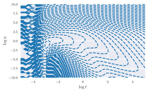
for some $h_{d}$ and $\delta_{d}$ small. We can use this observation to build a more efficient approximation. Let $\tilde{h}_{1}(\cdot)$ and $\tilde{h}_{2}(\cdot)$ denote interpolations at Chebyshev nodes of the functions $g(\cdot,0.5)$ and $g(0.5,\cdot)$. Then run Algorithm 5 with the target function $\frac{g(x_{1},x_{2})}{\tilde{h}_{1}(x_{1})\tilde{h}_{2}(x_{2})}$ and the error function $f_{\varepsilon}(y,\tilde{y},x_{1},x_{2})=\left\lvert(y-\tilde{y})\tilde{h}_{1}(x_{1})\tilde{h}_{2}(x_{2})\right\rvert$.

Example 4.1.

(Example 1.2 continued) I ran Algorithm 5 on the data set from Example 1.1. Figure 4 shows contours for the log of the reparameterized posterior function, and Figure 5 shows the sparse grid used to approximate the reparameterized posterior.

Figure 4: Reparameterized log posterior for the Example 1.1 data set with reference prior

Figure 5: Sparse grid used to interpolate the reparameterized posterior for the Example 1.1 data set with reference prior

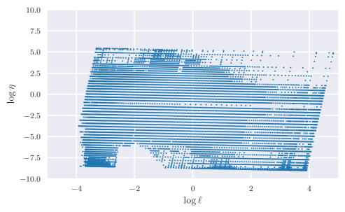
Prediction Distributions

The sparse grid from Algorithm 5 naturally leads to a quadrature rule to approximate integration (Jakeman, Roberts, 2011). Let $f(\ell,\eta)$ denote a function. Put $\boldsymbol{\varphi}(\boldsymbol{\mathrm{u}})=\left(\varphi_{\ell}(u_{1}),\varphi_{\eta}(u_{2})\right)^{\prime}$. Then

$$\int_{0}^{\infty}\int_{0}^{\infty} f(\ell,\eta)\operatorname{\pi}\left(\ell,\eta\mid\boldsymbol{\mathrm{y}}\right)d\ell d\eta$$

$$\approx\int_{0}^{\infty}\int_{0}^{\infty}f(\ell,\eta)\operatorname{\tilde{\pi}}\left(\ell,\eta\mid\boldsymbol{\mathrm{y}}\right)d\ell d\eta$$

$$\approx\!\begin{multlined}\frac{1}{Z}\int_{0}^{1}\int_{0}^{1}f\left(\boldsymbol{\varphi}(\boldsymbol{\mathrm{u}}_{\textrm{map}}+s_{1}(x_{1})\boldsymbol{\mathrm{v}}_{1}+s_{2}(x_{2})\boldsymbol{\mathrm{v}}_{2})\right)\\ g(x_{1},x_{2})\dot{s}_{1}(x_{1})\dot{s}_{2}(x_{2})dx_{1}dx_{2}\end{multlined}\frac{1}{Z}\int_{0}^{1}\int_{0}^{1}f\left(\boldsymbol{\varphi}(\boldsymbol{\mathrm{u}}_{\textrm{map}}+s_{1}(x_{1})\boldsymbol{\mathrm{v}}_{1}+s_{2}(x_{2})\boldsymbol{\mathrm{v}}_{2})\right)\\ g(x_{1},x_{2})\dot{s}_{1}(x_{1})\dot{s}_{2}(x_{2})dx_{1}dx_{2}$$ (13)

$$\approx\sum_{k}w_{k}f(\ell_{k},\eta_{k})$$ (14)

where the points $\left\{(\ell_{k},\eta_{k})^{\prime}\right\}$ are the transformed nodes of the sparse grid and weights are derived from integrals of the basis functions with the separable approximations,

$$\int_{0}^{1}\psi_{j}^{i}(x)\tilde{h}_{k}(x)dx$$

for $k=1,2$.

Let $\tilde{{\boldsymbol{s}}}$ denote unobserved locations. Then

$$\operatorname{P^{\pi}}\left(Z(\tilde{s}_{1}),\ldots,Z(\tilde{s}_{m})\mid\boldsymbol{\mathrm{y}}\right)\approx\sum_{k}w_{k}\operatorname{P^{\pi}}\left(Z(\tilde{s}_{1}),\ldots,Z(\tilde{s}_{m})\mid\boldsymbol{\mathrm{y}},\ell_{k},\eta_{k}\right)$$

gives us an approximation of the prediction distribution. Let’s derive a more explicit formula for the conditional probability $\operatorname{P^{\pi}}\left(\cdot\mid\boldsymbol{\mathrm{y}},\ell,\eta\right)$. Use $\boldsymbol{\mathrm{y}}_{1}=\boldsymbol{\mathrm{y}}$ to denote the observations and use $\boldsymbol{\mathrm{y}}_{2}$ to denote possible values at the unobserved locations $\tilde{s}_{1},\ldots,\tilde{s}_{m}$. Applying (3), we have

$$\operatorname{P^{\pi}}\left(\boldsymbol{\mathrm{y}}_{2}\mid\boldsymbol{\mathrm{y}}_{1},\ell,\eta\right) \propto\int_{0}^{\infty}\int_{\mathbb{R}^{p}}\operatorname{P}\left(\boldsymbol{\mathrm{y}}_{1},\boldsymbol{\mathrm{y}}_{2}\mid\boldsymbol{\beta},\sigma^{2},\ell,\eta\right)\left(\frac{1}{\sigma^{2}}\right)d\boldsymbol{\beta}d\sigma^{2}$$

$$\propto\left[\left(\boldsymbol{\mathrm{y}}_{1},\boldsymbol{\mathrm{y}}_{2}\right)\boldsymbol{R}\left(\boldsymbol{\mathrm{y}}_{1},\boldsymbol{\mathrm{y}}_{2}\right)^{\prime}\right]^{-(n+m-p)/2},$$

where $\boldsymbol{R}$ is given by (4). Put $\boldsymbol{R}=\begin{pmatrix}\boldsymbol{R}_{11}&\boldsymbol{R}_{12}\\ \boldsymbol{R}_{12}^{\prime}&\boldsymbol{R}_{22}\end{pmatrix}$. Then

$$\left(\boldsymbol{\mathrm{y}}_{1},\boldsymbol{\mathrm{y}}_{2}\right)\boldsymbol{R}\left(\boldsymbol{\mathrm{y}}_{1},\boldsymbol{\mathrm{y}}_{2}\right)^{\prime} =\boldsymbol{\mathrm{y}}_{1}^{\prime}\boldsymbol{R}_{11}\boldsymbol{\mathrm{y}}_{1}+2\boldsymbol{\mathrm{y}}_{1}^{\prime}\boldsymbol{R}_{12}\boldsymbol{\mathrm{y}}_{2}+\boldsymbol{\mathrm{y}}_{2}^{\prime}\boldsymbol{R}_{22}\boldsymbol{\mathrm{y}}_{2}$$

$$=\left(\boldsymbol{\mathrm{y}}_{2}-\bar{\boldsymbol{\mathrm{y}}}_{2}\right)^{\prime}\boldsymbol{R}_{22}\left(\boldsymbol{\mathrm{y}}_{2}-\bar{\boldsymbol{\mathrm{y}}}_{2}\right)+b$$

where $\bar{\boldsymbol{\mathrm{y}}}_{2}=-\boldsymbol{R}_{22}^{-1}\boldsymbol{R}_{12}^{\prime}\boldsymbol{\mathrm{y}}_{1}$ and $b=\boldsymbol{\mathrm{y}}_{1}^{\prime}\boldsymbol{R}_{11}\boldsymbol{\mathrm{y}}_{1}-\bar{\boldsymbol{\mathrm{y}}}_{2}^{\prime}\boldsymbol{R}_{22}\bar{\boldsymbol{\mathrm{y}}}_{2}$.

$\sigma^{2}$ Marginal

The marginal distribution of $\sigma^{2}$ is given by

$$\operatorname{P^{\pi}}\left(\sigma^{2}\mid\boldsymbol{\mathrm{y}}\right) =\int_{0}^{\infty}\int_{0}^{\infty}\operatorname{P^{\pi}}\left(\sigma^{2}\mid\boldsymbol{\mathrm{y}},\ell,\eta\right)\operatorname{\pi}\left(\ell,\eta\mid\boldsymbol{\mathrm{y}}\right)d\ell d\eta$$

$$\approx\sum_{k}w_{k}\operatorname{P^{\pi}}\left(\sigma^{2}\mid\boldsymbol{\mathrm{y}},\ell_{k},\eta_{k}\right),$$

where $\left\{w_{k}\right\}$, $\left\{\ell_{k}\right\}$, and $\left\{\eta_{k}\right\}$ are defined in (14). From (3), we have

$$\operatorname{P^{\pi}}\left(\sigma^{2}\mid\boldsymbol{\mathrm{y}},\ell,\eta\right) \propto\int_{\mathbb{R}^{p}}L(\boldsymbol{\beta},\sigma^{2},\ell,\eta;\boldsymbol{\mathrm{y}})\operatorname{\pi}\left(\boldsymbol{\beta},\sigma^{2}\mid\ell,\eta\right)d\boldsymbol{\beta}$$

$$\propto\left(\sigma^{2}\right)^{-(n-p)/2}\lvert\boldsymbol{\mathrm{G}}\rvert^{-1/2}\lvert\boldsymbol{\mathrm{X}}^{\prime}\boldsymbol{\mathrm{G}}^{-1}\boldsymbol{\mathrm{X}}\rvert^{-1/2}\exp\left\{-\frac{S^{2}}{2\sigma^{2}}\right\}\left(\frac{1}{\sigma^{2}}\right)$$

$$\propto\left(\frac{1}{\sigma^{2}}\right)^{(n-p)/2+1}\exp\left\{-\frac{S^{2}}{2\sigma^{2}}\right\}.$$ (15)

(15) is the unnormalized PDF of an inverse-gamma distribution. Normalizing gives us

$$\operatorname{P^{\pi}}\left(\sigma^{2}\mid\boldsymbol{\mathrm{y}},\ell,\eta\right)=\frac{\left(S^{2}/2\right)^{(n-p)/2}}{\Gamma((n-p)/2)}\left(\frac{1}{\sigma^{2}}\right)^{(n-p)/2+1}\exp\left\{-\frac{S^{2}}{2\sigma^{2}}\right\}.$$

$\boldsymbol{\beta}$ Marginals

Similarly, to compute the posterior distribution of a particular regressor $\beta_{j}$, we have

$$\operatorname{P^{\pi}}\left(\beta_{j}\mid\boldsymbol{\mathrm{y}}\right) =\int_{0}^{\infty}\int_{0}^{\infty}\operatorname{P^{\pi}}\left(\beta_{j}\mid\boldsymbol{\mathrm{y}},\ell,\eta\right)\operatorname{\pi}\left(\ell,\eta\mid\boldsymbol{\mathrm{y}}\right)d\ell d\eta$$

where

$$\operatorname{P^{\pi}}\left(\beta_{j}\mid\boldsymbol{\mathrm{y}},\ell,\eta\right) \propto\begin{multlined}\int_{0}^{\infty}\int_{\mathbb{R}^{p-1}}\left(\frac{1}{\sigma^{2}}\right)^{n/2+1}\\ \exp\left\{-\frac{1}{2\sigma^{2}}\left(\boldsymbol{\mathrm{y}}-\boldsymbol{\mathrm{X}}\boldsymbol{\beta}\right)^{\prime}\boldsymbol{\mathrm{G}}^{-1}\left(\boldsymbol{\mathrm{y}}-\boldsymbol{\mathrm{X}}\boldsymbol{\beta}\right)\right\}d\boldsymbol{\beta}_{/j}d\sigma^{2}\end{multlined}\int_{0}^{\infty}\int_{\mathbb{R}^{p-1}}\left(\frac{1}{\sigma^{2}}\right)^{n/2+1}\\ \exp\left\{-\frac{1}{2\sigma^{2}}\left(\boldsymbol{\mathrm{y}}-\boldsymbol{\mathrm{X}}\boldsymbol{\beta}\right)^{\prime}\boldsymbol{\mathrm{G}}^{-1}\left(\boldsymbol{\mathrm{y}}-\boldsymbol{\mathrm{X}}\boldsymbol{\beta}\right)\right\}d\boldsymbol{\beta}_{/j}d\sigma^{2}$$

$$\propto\begin{multlined}\int_{0}^{\infty}\int_{\mathbb{R}^{p-1}}\left(\frac{1}{\sigma^{2}}\right)^{n/2+1}\\ \exp\left\{-\frac{1}{2\sigma^{2}}\left(\boldsymbol{\beta}-\bar{\boldsymbol{\beta}}\right)^{\prime}\boldsymbol{\mathrm{X}}^{\prime}\boldsymbol{\mathrm{G}}^{-1}\boldsymbol{\mathrm{X}}\left(\boldsymbol{\beta}-\bar{\boldsymbol{\beta}}\right)\right\}\\ \exp\left\{-\frac{1}{2\sigma^{2}}\left(\boldsymbol{\mathrm{y}}^{\prime}\boldsymbol{\mathrm{G}}^{-1}\boldsymbol{\mathrm{y}}-\bar{\boldsymbol{\beta}}\boldsymbol{\mathrm{X}}^{\prime}\boldsymbol{\mathrm{G}}^{-1}\boldsymbol{\mathrm{X}}\bar{\boldsymbol{\beta}}\right)\right\}d\boldsymbol{\beta}_{/j}d\sigma^{2}\end{multlined}\int_{0}^{\infty}\int_{\mathbb{R}^{p-1}}\left(\frac{1}{\sigma^{2}}\right)^{n/2+1}\\ \exp\left\{-\frac{1}{2\sigma^{2}}\left(\boldsymbol{\beta}-\bar{\boldsymbol{\beta}}\right)^{\prime}\boldsymbol{\mathrm{X}}^{\prime}\boldsymbol{\mathrm{G}}^{-1}\boldsymbol{\mathrm{X}}\left(\boldsymbol{\beta}-\bar{\boldsymbol{\beta}}\right)\right\}\\ \exp\left\{-\frac{1}{2\sigma^{2}}\left(\boldsymbol{\mathrm{y}}^{\prime}\boldsymbol{\mathrm{G}}^{-1}\boldsymbol{\mathrm{y}}-\bar{\boldsymbol{\beta}}\boldsymbol{\mathrm{X}}^{\prime}\boldsymbol{\mathrm{G}}^{-1}\boldsymbol{\mathrm{X}}\bar{\boldsymbol{\beta}}\right)\right\}d\boldsymbol{\beta}_{/j}d\sigma^{2}$$

$$\propto\begin{multlined}\int_{0}^{\infty}\left(\frac{1}{\sigma^{2}}\right)^{(n-p+1)/2+1}\exp\left\{-\frac{1}{2\sigma^{2}}\frac{1}{\left(\boldsymbol{A}^{-1}\right)_{jj}}\left(\beta_{j}-\bar{\beta}_{j}\right)^{2}\right\}\\ \exp\left\{-\frac{1}{2\sigma^{2}}\left(\boldsymbol{\mathrm{y}}^{\prime}\boldsymbol{\mathrm{G}}^{-1}\boldsymbol{\mathrm{y}}-\bar{\boldsymbol{\beta}}\boldsymbol{\mathrm{X}}^{\prime}\boldsymbol{\mathrm{G}}^{-1}\boldsymbol{\mathrm{X}}\bar{\boldsymbol{\beta}}\right)\right\}d\sigma^{2}\end{multlined}\int_{0}^{\infty}\left(\frac{1}{\sigma^{2}}\right)^{(n-p+1)/2+1}\exp\left\{-\frac{1}{2\sigma^{2}}\frac{1}{\left(\boldsymbol{A}^{-1}\right)_{jj}}\left(\beta_{j}-\bar{\beta}_{j}\right)^{2}\right\}\\ \exp\left\{-\frac{1}{2\sigma^{2}}\left(\boldsymbol{\mathrm{y}}^{\prime}\boldsymbol{\mathrm{G}}^{-1}\boldsymbol{\mathrm{y}}-\bar{\boldsymbol{\beta}}\boldsymbol{\mathrm{X}}^{\prime}\boldsymbol{\mathrm{G}}^{-1}\boldsymbol{\mathrm{X}}\bar{\boldsymbol{\beta}}\right)\right\}d\sigma^{2}$$

$$\propto\int_{0}^{\infty}\left(\frac{1}{\sigma^{2}}\right)^{(n-p+1)/2+1}\exp\left\{-\frac{1}{2\sigma^{2}}\#1\right\}d\sigma^{2}$$

$$\propto\left(\#1\right)^{-(n-p+1)/2}$$

and

$$\boldsymbol{A} =\boldsymbol{\mathrm{X}}^{\prime}\boldsymbol{\mathrm{G}}^{-1}\boldsymbol{\mathrm{X}}$$

$$\bar{\beta} =\boldsymbol{A}^{-1}\boldsymbol{\mathrm{X}}^{\prime}\boldsymbol{\mathrm{G}}^{-1}\boldsymbol{\mathrm{y}}$$

$$\#1 =\frac{1}{\left(\boldsymbol{A}^{-1}\right)_{jj}}\left(\beta_{j}-\bar{\beta}_{j}\right)^{2}+\boldsymbol{\mathrm{y}}^{\prime}\boldsymbol{\mathrm{G}}^{-1}\boldsymbol{\mathrm{y}}-\bar{\boldsymbol{\beta}}^{\prime}\boldsymbol{A}\bar{\boldsymbol{\beta}}$$

$$=\frac{1}{\left(\boldsymbol{A}^{-1}\right)_{jj}}\left(\beta_{j}-\bar{\beta}_{j}\right)^{2}+S^{2}.$$

We recognize $\operatorname{P^{\pi}}\left(\beta_{j}\mid\boldsymbol{\mathrm{y}}\right)$ as being a t-distribution with $n-p$ degrees of freedom, mean $\boldsymbol{\beta}_{j}$, and scale $s_{\beta_{j}}=\left\{\frac{\left(\boldsymbol{A}^{-1}\right)_{jj}S^{2}}{n-p}\right\}^{1/2}$.

$\ell$, $\eta$ Marginals

Algorithm 5 gives us an interpolating function that is inexpensive to evaluate and accurately approximates the reparameterized posterior $\operatorname{\pi}\left(u_{1},u_{2}\mid\boldsymbol{\mathrm{y}}\right)=\operatorname{\pi}\left(\varphi_{\ell}(u_{1}),\varphi_{\eta}(u_{2})\mid\boldsymbol{\mathrm{y}}\right)\dot{\varphi}_{\ell}(u_{1})\dot{\varphi}_{\eta}(u_{2})$. Now,

$$\operatorname{\pi}\left(u_{1}\mid\boldsymbol{\mathrm{y}}\right) =\int\operatorname{\pi}\left(u_{1},u_{2}\mid\boldsymbol{\mathrm{y}}\right)du_{2}$$

$$\approx\sum_{k}w_{k}\operatorname{\tilde{\pi}}\left(u_{1},t_{k}\mid\boldsymbol{\mathrm{y}}\right),$$

where $\left\{w_{k}\right\}$ and $\left\{t_{k}\right\}$ can be chosen by the Gauss-Legendre quadrature rule for the interval determined by the bracketing region in Step 2 of Algorithm 3. If we evaluate $\operatorname{\tilde{\pi}}\left(u_{1}\mid\boldsymbol{\mathrm{y}}\right)$ at Chebyshev nodes across the range of $u_{1}$ in the bracketing region, then we obtain a polynomial that approximates $\operatorname{\pi}\left(u_{1}\mid\boldsymbol{\mathrm{y}}\right)$. $\operatorname{\pi}\left(u_{2}\mid\boldsymbol{\mathrm{y}}\right)$ can be similarly approximated using Chebyshev nodes.

If the error bounds from Step 2 are tight enough, the polynomial approximations for $\operatorname{\pi}\left(u_{1}\mid\boldsymbol{\mathrm{y}}\right)$ and $\operatorname{\pi}\left(u_{2}\mid\boldsymbol{\mathrm{y}}\right)$ will be suitable for estimating the CDFs. But since they cut off integration outside of the bracketing region, they won’t accurately capture endpoint behavior and shouldn’t be used for estimating moments. For example, $\operatorname{\pi}\left(\eta\mid\boldsymbol{\mathrm{y}}\right)$ has infinite mean, which won’t be reflected by the polynomial approximation.

5 Real Data Analysis

Let’s apply the algorithms from §4 to real data.

5.1 Soil Carbon-to-Nitrogen

We’ll first look at a data set from Schabenberger, Pierce (2001) of carbon-to-nitrogen ratios sampled across an agricultural field before and after tillage. The after-tillage data was analyzed by Ren et al. (2012) and De Oliveira (2007) using random sampling algorithms and a Gaussian process of the form (1) with

$$\operatorname{\mathbb{E}}\left\{Z({\boldsymbol{s}})\right\}=\beta_{1}\quad\text{and}\quad\operatorname{\psi}_{\ell}(d)=\exp\left\{-\frac{d}{\ell}\right\}.$$

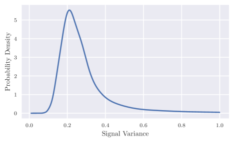
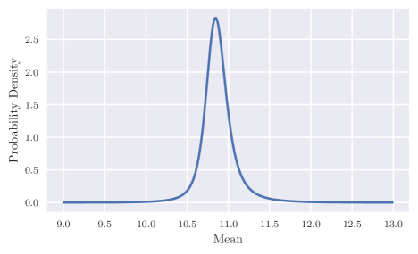
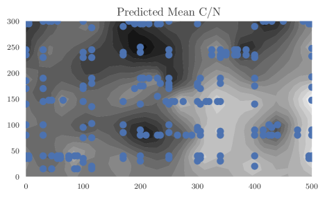
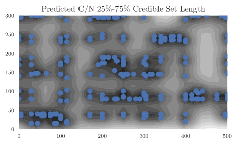
We’ll use the same model and data set with our deterministic algorithms. When we fit a sparse grid to approximate the posterior and marginalize, we get these values for the medians

$$\left(\beta_{1}\right)_{\textrm{med}}=10.86,\quad\ell_{\textrm{med}}=62.54,\quad\eta_{\textrm{med}}=0.44,\quad\textrm{and}\quad\sigma^{2}_{\textrm{med}}=0.24.$$

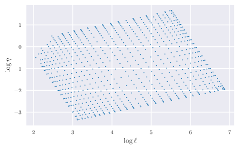
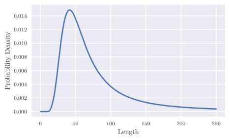
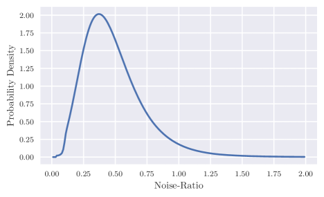
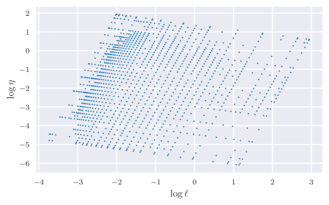
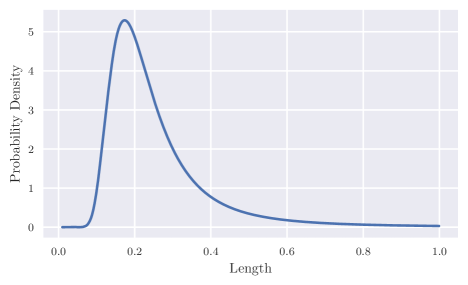
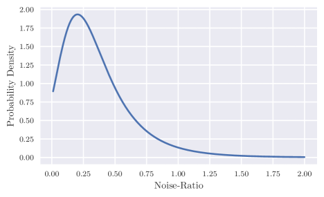
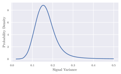
Figure 6 plots the sparse grid constructed by Algorithm 5; Figure 7 plots the posterior marginalizations for $\beta_{1}$, $\ell$, $\eta$, and $\sigma^{2}$; and Figure 8 plots carbon-to-nitrogen predictions and credible sets across the agricultural field. [source]

Figure 6: Sparse grid used to interpolate the posterior of the soil data set

Figure 7: Marginalizations of the posterior distribution of the soil data set

Figure 8: Prediction means and credible sets of soil carbon-to-nitrogen ratios for soil data set with sampling locations

5.2 Meuse River

Next, we’ll look at a data set from the sp R-library containing $\mathrm{155}$ measurements of zinc concentration (ppm) collected in a flood plain of the river Meuse (Pebesma, Bivand, 2005). The data was previously analyzed by Kazianka, Pilz (2012) using a Gaussian process with a sampling algorithm. We’ll use a similar model but with the deterministic algorithms from §4. We model log zinc concentration as a Gaussian process of the form (1) with

$$\operatorname{\mathbb{E}}\left\{Z({\boldsymbol{s}})\right\}=\beta_{1}+\beta_{2}x_{1}({\boldsymbol{s}})\quad\text{and}\quad\operatorname{\psi}_{\ell}(d)=\exp\left\{-\frac{d}{\ell}\right\}$$

where $x_{1}({\boldsymbol{s}})$ is the square root of the distance of the flood plain sampling location, ${\boldsymbol{s}}$, to the river Meuse. After fitting the model, we compute medians

$$\left(\beta_{1}\right)_{\textrm{med}}=6.99,\;\left(\beta_{2}\right)_{\textrm{med}}=-2.56,\;\ell_{\textrm{med}}=0.22,\;\eta_{\textrm{med}}=0.31,\;\textrm{and}\;\sigma^{2}_{\textrm{med}}=0.16.$$

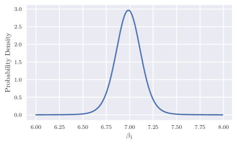
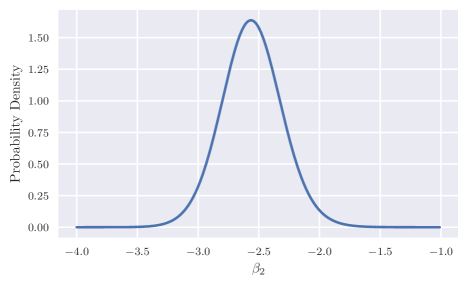
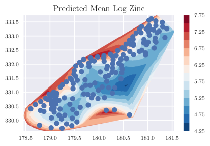
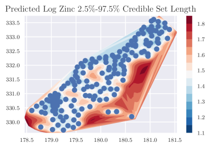
Figure 9 plots the sparse grid constructed by Algorithm 5; Figure 10 plots the posterior marginalizations for $\beta_{1}$, $\beta_{2}$, $\ell$, $\eta$, and $\sigma^{2}$; and Figure 11 plots log zinc predictions and credible sets across the flood plain. [source]

Figure 9: Sparse grid used to interpolate the posterior of the Meuse data set

Figure 10: Marginalizations of the posterior distribution of the Meuse data set

Figure 11: Prediction means and credible sets of log zinc concentration for Meuse data set with sampling locations

5.3 Performance Analysis

To get a sense of the cost of the algorithms, I measured how long it took to apply the steps of Algorithm 3 to the soil and Meuse data sets for varying error tolerances. I computed the results using an 8-core AMD Ryzen 9 laptop. Table 10 and Table 11 summarize the performance results and provide the 25th, 50th, and 75th percentiles for the $\ell$, $\eta$, and $\sigma^{2}$ distributions to help show how the tolerance affects accuracy. [source]

			$\ell$ Percentile			$\eta$ Percentile			$\sigma^{2}$ Percentile
tol	grid size	elapse (s)	25th	50th	75th	25th	50th	75th	25th	50th	75th
$\mathrm{1{}\times{}10^{-2}}$	249	1.37	42.00	63.50	106.92	0.31	0.45	0.60	0.20	0.25	0.31
$\mathrm{1{}\times{}10^{-3}}$	252	1.32	42.88	62.55	104.56	0.32	0.44	0.61	0.20	0.25	0.32
$\mathrm{1{}\times{}10^{-4}}$	798	2.86	42.88	62.55	104.56	0.32	0.44	0.61	0.20	0.25	0.32
$\mathrm{1{}\times{}10^{-5}}$	2218	6.67	42.88	62.54	104.57	0.32	0.44	0.61	0.20	0.25	0.32
$\mathrm{1{}\times{}10^{-6}}$	3415	9.82	42.88	62.54	104.57	0.32	0.44	0.61	0.20	0.25	0.32

Table 10: Provide distribution percentiles and measure elapse time for fitting a sparse grid to the soil data set described in §5.1 using various tolerances

			$\ell$ Percentile			$\eta$ Percentile			$\sigma^{2}$ Percentile
tol	grid size	elapse (s)	25th	50th	75th	25th	50th	75th	25th	50th	75th
$\mathrm{1{}\times{}10^{-2}}$	215	0.69	0.17	0.22	0.30	0.17	0.31	0.50	0.13	0.16	0.20
$\mathrm{1{}\times{}10^{-3}}$	416	1.03	0.17	0.22	0.30	0.17	0.31	0.49	0.13	0.16	0.20
$\mathrm{1{}\times{}10^{-4}}$	1193	2.42	0.17	0.22	0.30	0.17	0.31	0.50	0.13	0.16	0.20
$\mathrm{1{}\times{}10^{-5}}$	2358	4.51	0.17	0.22	0.30	0.17	0.31	0.50	0.13	0.16	0.20
$\mathrm{1{}\times{}10^{-6}}$	8666	17.10	0.17	0.22	0.30	0.17	0.31	0.50	0.13	0.16	0.20

Table 11: Provide distribution percentiles and measure elapse time for fitting a sparse grid to the Meuse data set described in §5.2 using various tolerances

6 Discussion

I presented deterministic algorithms for fully Bayesian prediction and inference for spatial models. In comparison to sampling methods such as MCMC, I would expect the algorithms to provide more reproducible results and require less tuning, making a more turnkey approach to analysis possible.

An area of future work could be to extend the algorithms to handle the Gaussian process models used in model emulation and calibration. In contrast to spatial Gaussian process models, models for emulation and calibration typically assume each dimension of the input space has a different scale and use a product covariance function (Sacks et al., 1989; Gu, 2019),

$$\operatorname{cov}\left\{Z({\boldsymbol{s}}),Z(\boldsymbol{\mathrm{u}})\right\} =\sigma^{2}\prod_{k=1}^{d}\psi_{\ell_{k}}(\mid s_{k}-u_{k}\mid).$$

Paulo (2005) and Gu, Berger (2016) derived reference priors for separable covariance functions with distinct length parameters. Provided $d$ is not too large, it may be possible to adopt the algorithms from §4 to work for this case to achieve deterministic fully Bayesian results. Additionally, certain modifications, such as using second-order information at interpolation points or assuming that the posterior is separable along the eigenvectors of its optimum’s Hessian, could make the algorithms more efficient and larger values of $d$ possible.

Appendix A Appendix: Posterior Derivatives

We will derive equations to compute the value, gradient, and Hessian of the negative log posterior $\operatorname{\pi}\left(\ell,\eta\mid\boldsymbol{\mathrm{y}}\right)$. From (3) and (5), we have

$$\operatorname{\pi}\left(\ell,\eta\mid\boldsymbol{\mathrm{y}}\right) \propto L^{I}(\ell,\eta;\boldsymbol{\mathrm{y}})\times\operatorname{\pi}\left(\ell,\eta\right)$$

$$\propto\lvert\boldsymbol{\mathrm{G}}\rvert^{-1/2}\lvert\boldsymbol{\mathrm{X}}^{\prime}\boldsymbol{\mathrm{G}}^{-1}\boldsymbol{\mathrm{X}}\rvert^{-1/2}\left(S^{2}\right)^{-(n-p)/2}\lvert\boldsymbol{\Sigma}\rvert^{1/2}.$$

Put $\phi_{1}=\ell$, $\phi_{2}=\eta$, $\boldsymbol{A}=\boldsymbol{\mathrm{X}}^{\prime}\boldsymbol{\mathrm{G}}^{-1}\boldsymbol{\mathrm{X}}$, and define

$$f(\boldsymbol{\phi})=\frac{1}{2}\log\lvert\boldsymbol{\mathrm{G}}\rvert+\frac{1}{2}\log\lvert\boldsymbol{A}\rvert+\frac{n-p}{2}\log S^{2}-\frac{1}{2}\log{\lvert\boldsymbol{\Sigma}\rvert}.$$

Let $\boldsymbol{L}_{G}$ denote the Cholesky factorization of $\boldsymbol{\mathrm{G}}$, $\boldsymbol{\mathrm{G}}=\boldsymbol{L}_{G}\boldsymbol{L}_{G}^{\prime}$. Then

$$\boldsymbol{A} =\boldsymbol{\mathrm{X}}^{\prime}\left(\boldsymbol{L}_{G}\boldsymbol{L}_{G}^{\prime}\right)^{-1}\boldsymbol{\mathrm{X}}$$

$$=\boldsymbol{\mathrm{X}}^{\prime}\boldsymbol{L}_{G}^{\prime-1}\boldsymbol{L}_{G}^{-1}\boldsymbol{\mathrm{X}}$$

$$=\left(\boldsymbol{L}_{G}^{-1}\boldsymbol{\mathrm{X}}\right)^{\prime}\left(\boldsymbol{L}_{G}^{-1}\boldsymbol{\mathrm{X}}\right).$$

Let $\boldsymbol{\mathrm{Q}}$ and $\boldsymbol{R}_{A}$ denote the QR factorization of $\boldsymbol{L}_{G}^{-1}\boldsymbol{\mathrm{X}}$. Then

$$\boldsymbol{A} =\left(\boldsymbol{L}_{G}^{-1}\boldsymbol{\mathrm{X}}\right)^{\prime}\left(\boldsymbol{L}_{G}^{-1}\boldsymbol{\mathrm{X}}\right)$$

$$=\left(\boldsymbol{\mathrm{Q}}\boldsymbol{R}_{A}\right)^{\prime}\left(\boldsymbol{\mathrm{Q}}\boldsymbol{R}_{A}\right)$$

$$=\boldsymbol{R}_{A}^{\prime}\boldsymbol{\mathrm{Q}}^{\prime}\boldsymbol{\mathrm{Q}}\boldsymbol{R}_{A}$$

$$=\boldsymbol{R}_{A}^{\prime}\boldsymbol{R}_{A}.$$

Put $\boldsymbol{\mathrm{H}}=\boldsymbol{\mathrm{G}}^{-1}\boldsymbol{\mathrm{X}}\boldsymbol{A}^{-1}\boldsymbol{\mathrm{X}}^{\prime}\boldsymbol{\mathrm{G}}^{-1}$ and $\boldsymbol{F}_{H}=\boldsymbol{R}_{A}^{\prime-1}\boldsymbol{\mathrm{X}}^{\prime}\boldsymbol{\mathrm{G}}^{-1}$. Applying to $\boldsymbol{R}$ (4), we have $\boldsymbol{\mathrm{H}}=\boldsymbol{F}_{H}^{\prime}\boldsymbol{F}_{H}$ and $\boldsymbol{R}=\boldsymbol{L}_{G}^{\prime-1}\boldsymbol{L}_{G}^{-1}+\boldsymbol{F}_{H}^{\prime}\boldsymbol{F}_{H}$.

Gradient

Put

$$\#1=\frac{1}{2}\log\lvert\boldsymbol{\mathrm{G}}\rvert,\quad\#2=\frac{1}{2}\log\lvert\boldsymbol{A}\rvert,\quad\#3=\frac{n-p}{2}\log S^{2},\ \text{and}\quad\#4=\frac{1}{2}\log\lvert\boldsymbol{\Sigma}\rvert.$$

Applying Jacobi’s formula, $\frac{d}{dt}\lvert\boldsymbol{B}(t)\rvert=\lvert\boldsymbol{B}\rvert\operatorname{tr}\left\{\boldsymbol{B}^{-1}\frac{d\boldsymbol{B}}{dt}\right\}$, we have

$$\frac{\partial\#1}{\partial\phi_{s}} =\frac{1}{2}\operatorname{tr}\left\{\boldsymbol{\mathrm{G}}^{-1}\frac{\partial\boldsymbol{\mathrm{G}}}{\partial\phi_{s}}\right\},$$

$$\frac{\partial\#2}{\partial\phi_{s}} =\frac{1}{2}\operatorname{tr}\left\{\boldsymbol{A}^{-1}\frac{\partial\boldsymbol{A}}{\partial\phi_{s}}\right\},$$

$$\frac{\partial\#3}{\partial\phi_{s}} =\frac{n-p}{2}\frac{1}{S^{2}}\frac{\partial S^{2}}{\partial\phi_{s}}=\frac{n-p}{2}\frac{1}{S^{2}}\boldsymbol{\mathrm{y}}^{\prime}\frac{\partial\boldsymbol{R}}{\partial\phi_{s}}\boldsymbol{\mathrm{y}},$$

$$\frac{\partial\#4}{\partial\phi_{s}} =\frac{1}{2}\operatorname{tr}\left\{\boldsymbol{\Sigma}^{-1}\frac{\partial\boldsymbol{\Sigma}}{\partial\phi_{s}}\right\}.$$

Using the formula for differentiating an inverse matrix, $\frac{d}{dt}\boldsymbol{B}(t)^{-1}=-\boldsymbol{B}^{-1}\frac{d\boldsymbol{B}}{dt}\boldsymbol{B}^{-1}$, we derive the derivative of $\boldsymbol{A}$,

$$\frac{\partial\boldsymbol{A}}{\partial\phi_{s}}=\boldsymbol{\mathrm{X}}^{\prime}\frac{\partial\boldsymbol{\mathrm{G}}^{-1}}{\partial\phi_{s}}\boldsymbol{\mathrm{X}}$$

where $\frac{\partial\boldsymbol{\mathrm{G}}^{-1}}{\partial\phi_{s}}=-\boldsymbol{\mathrm{G}}^{-1}\frac{\partial\boldsymbol{\mathrm{G}}}{\partial\phi_{s}}\boldsymbol{\mathrm{G}}^{-1}$. Differentiating $\boldsymbol{R}$ gives us

$$\frac{\partial\boldsymbol{R}}{\partial\phi_{s}}=\frac{\partial}{\partial\phi_{s}}\left(\boldsymbol{\mathrm{G}}^{-1}-\boldsymbol{\mathrm{H}}\right)=\frac{\partial\boldsymbol{\mathrm{G}}^{-1}}{\partial\phi_{s}}-\frac{\partial\boldsymbol{\mathrm{H}}}{\partial\phi_{s}}$$

and

$$\frac{\partial\boldsymbol{\mathrm{H}}}{\partial\phi_{s}} =\frac{\partial}{\partial\phi_{s}}\left(\boldsymbol{\mathrm{G}}^{-1}\boldsymbol{\mathrm{X}}\boldsymbol{A}^{-1}\boldsymbol{\mathrm{X}}^{\prime}\boldsymbol{\mathrm{G}}^{-1}\right)$$

$$=-\boldsymbol{\mathrm{G}}^{-1}\frac{\partial\boldsymbol{\mathrm{G}}}{\partial\phi_{s}}\boldsymbol{\mathrm{H}}-\boldsymbol{\mathrm{H}}\frac{\partial\boldsymbol{\mathrm{G}}}{\partial\phi_{s}}\boldsymbol{\mathrm{G}}^{-1}-\boldsymbol{\mathrm{G}}^{-1}\boldsymbol{\mathrm{X}}\boldsymbol{A}^{-1}\frac{\partial\boldsymbol{A}}{\partial\phi_{s}}\boldsymbol{A}^{-1}\boldsymbol{\mathrm{X}}\boldsymbol{\mathrm{G}}^{-1}$$

$$=\!\begin{multlined}-\boldsymbol{\mathrm{G}}^{-1}\frac{\partial\boldsymbol{\mathrm{G}}}{\partial\phi_{s}}\boldsymbol{\mathrm{H}}-\boldsymbol{\mathrm{H}}\frac{\partial\boldsymbol{\mathrm{G}}}{\partial\phi_{s}}\boldsymbol{\mathrm{G}}^{-1}\\ +\boldsymbol{\mathrm{G}}^{-1}\boldsymbol{\mathrm{X}}\boldsymbol{A}^{-1}\left(\boldsymbol{\mathrm{X}}^{\prime}\boldsymbol{\mathrm{G}}^{-1}\frac{\partial\boldsymbol{\mathrm{G}}}{\partial\phi_{s}}\boldsymbol{\mathrm{G}}^{-1}\boldsymbol{\mathrm{X}}\right)\boldsymbol{A}^{-1}\boldsymbol{\mathrm{X}}\boldsymbol{\mathrm{G}}^{-1}\end{multlined}-\boldsymbol{\mathrm{G}}^{-1}\frac{\partial\boldsymbol{\mathrm{G}}}{\partial\phi_{s}}\boldsymbol{\mathrm{H}}-\boldsymbol{\mathrm{H}}\frac{\partial\boldsymbol{\mathrm{G}}}{\partial\phi_{s}}\boldsymbol{\mathrm{G}}^{-1}\\ +\boldsymbol{\mathrm{G}}^{-1}\boldsymbol{\mathrm{X}}\boldsymbol{A}^{-1}\left(\boldsymbol{\mathrm{X}}^{\prime}\boldsymbol{\mathrm{G}}^{-1}\frac{\partial\boldsymbol{\mathrm{G}}}{\partial\phi_{s}}\boldsymbol{\mathrm{G}}^{-1}\boldsymbol{\mathrm{X}}\right)\boldsymbol{A}^{-1}\boldsymbol{\mathrm{X}}\boldsymbol{\mathrm{G}}^{-1}$$

$$=-\boldsymbol{\mathrm{G}}^{-1}\frac{\partial\boldsymbol{\mathrm{G}}}{\partial\phi_{s}}\boldsymbol{\mathrm{H}}-\boldsymbol{\mathrm{H}}\frac{\partial\boldsymbol{\mathrm{G}}}{\partial\phi_{s}}\boldsymbol{\mathrm{G}}^{-1}+\boldsymbol{\mathrm{H}}\frac{\partial\boldsymbol{\mathrm{G}}}{\partial\phi_{s}}\boldsymbol{\mathrm{H}}$$

$$=-\left(\boldsymbol{\mathrm{G}}^{-1}-\frac{1}{2}\boldsymbol{\mathrm{H}}\right)\frac{\partial\boldsymbol{\mathrm{G}}}{\partial\phi_{s}}\boldsymbol{\mathrm{H}}-\boldsymbol{\mathrm{H}}\frac{\partial\boldsymbol{\mathrm{G}}}{\partial\phi_{s}}\left(\boldsymbol{\mathrm{G}}^{-1}-\frac{1}{2}\boldsymbol{\mathrm{H}}\right).$$

Put $\#5=\operatorname{tr}\left\{\boldsymbol{R}\frac{\partial\boldsymbol{\mathrm{K}}}{\partial\ell}\right\}$. Then

$$\left(\frac{\partial\boldsymbol{\Sigma}}{\partial\phi_{s}}\right)_{11} =\frac{\partial}{\partial\phi_{s}}\operatorname{tr}\left\{\#5^{2}\right\}=2\operatorname{tr}\left\{\#5\frac{\partial\#5}{\partial\phi_{s}}\right\},$$

$$\left(\frac{\partial\boldsymbol{\Sigma}}{\partial\phi_{s}}\right)_{12} =\frac{\partial}{\partial\phi_{s}}\operatorname{tr}\left\{\boldsymbol{R}^{2}\frac{\partial\boldsymbol{\mathrm{K}}}{\partial\ell}\right\}=\operatorname{tr}\left\{\frac{\partial\boldsymbol{R}^{2}}{\partial\phi_{s}}\frac{\partial\boldsymbol{\mathrm{K}}}{\partial\ell}+\boldsymbol{R}^{2}\frac{\partial^{2}\boldsymbol{\mathrm{K}}}{\partial\phi_{s}\partial\ell}\right\},$$

$$\left(\frac{\partial\boldsymbol{\Sigma}}{\partial\phi_{s}}\right)_{13} =\operatorname{tr}\left\{\frac{\partial\#5}{\partial\phi_{s}}\right\},$$

$$\left(\frac{\partial\boldsymbol{\Sigma}}{\partial\phi_{s}}\right)_{22} =\operatorname{tr}\left\{\frac{\partial\boldsymbol{R}^{2}}{\partial\phi_{s}}\right\},$$

$$\left(\frac{\partial\boldsymbol{\Sigma}}{\partial\phi_{s}}\right)_{23} =\operatorname{tr}\left\{\frac{\partial\boldsymbol{R}}{\partial\phi_{s}}\right\},$$

$$\left(\frac{\partial\boldsymbol{\Sigma}}{\partial\phi_{s}}\right)_{33} =0,$$

and

$$\frac{\partial\#5}{\partial\phi_{s}} =\frac{\partial}{\partial\phi_{s}}\left(\boldsymbol{R}\frac{\partial\boldsymbol{\mathrm{K}}}{\partial\ell}\right)=\frac{\partial\boldsymbol{R}}{\partial\phi_{s}}\frac{\partial\boldsymbol{\mathrm{K}}}{\partial\ell}+\boldsymbol{R}\frac{\partial^{2}\boldsymbol{\mathrm{K}}}{\partial\phi_{s}\partial\ell}$$

$$\frac{\partial\boldsymbol{R}^{2}}{\partial\phi_{s}} =\frac{\partial\boldsymbol{R}}{\partial\phi_{s}}\boldsymbol{R}+\boldsymbol{R}\frac{\partial\boldsymbol{R}}{\partial\phi_{s}}.$$

Hessian

Computing second derivatives we have

$$\frac{\partial^{2}\#1}{\partial\phi_{s}\partial\phi_{t}} =\frac{\partial}{\partial\phi_{s}}\left(\frac{1}{2}\operatorname{tr}\left\{\boldsymbol{\mathrm{G}}^{-1}\frac{\partial\boldsymbol{\mathrm{G}}}{\partial\phi_{t}}\right\}\right)$$

$$=\frac{1}{2}\operatorname{tr}\left\{-\boldsymbol{\mathrm{G}}^{-1}\frac{\partial\boldsymbol{\mathrm{G}}}{\partial\phi_{s}}\boldsymbol{\mathrm{G}}^{-1}\frac{\partial\boldsymbol{\mathrm{G}}}{\partial\phi_{t}}+\boldsymbol{\mathrm{G}}^{-1}\frac{\partial^{2}\boldsymbol{\mathrm{G}}}{\partial\phi_{s}\partial\phi_{t}}\right\},$$

$$\frac{\partial^{2}\#2}{\partial\phi_{s}\partial\phi_{t}} =\frac{\partial}{\partial\phi_{s}}\left(\frac{1}{2}\operatorname{tr}\left\{\boldsymbol{A}^{-1}\frac{\partial\boldsymbol{A}}{\partial\phi_{t}}\right\}\right)$$

$$=\frac{1}{2}\operatorname{tr}\left\{-\boldsymbol{A}^{-1}\frac{\partial\boldsymbol{A}}{\partial\phi_{s}}\boldsymbol{A}^{-1}\frac{\partial\boldsymbol{A}}{\partial\phi_{t}}+\boldsymbol{A}^{-1}\frac{\partial^{2}\boldsymbol{A}}{\partial\phi_{s}\partial\phi_{t}}\right\},$$

$$\frac{\partial^{2}\#3}{\partial\phi_{s}\partial\phi_{t}} =\frac{\partial}{\partial\phi_{s}}\left(\frac{n-p}{2}\frac{1}{S^{2}}\frac{\partial S^{2}}{\partial\phi_{t}}\right)$$

$$=\frac{n-p}{2}\left(-\frac{1}{S^{4}}\frac{\partial S^{2}}{\partial\phi_{s}}\frac{\partial S^{2}}{\partial\phi_{t}}+\frac{1}{S^{2}}\frac{\partial^{2}S^{2}}{\partial\phi_{s}\partial\phi_{t}}\right),$$

$$\frac{\partial^{2}\#4}{\partial\phi_{s}\partial\phi_{t}} =\frac{\partial}{\partial\phi_{s}}\left(\frac{1}{2}\operatorname{tr}\left\{\boldsymbol{\Sigma}^{-1}\frac{\partial\boldsymbol{\Sigma}}{\partial\phi_{t}}\right\}\right)$$

$$=\frac{1}{2}\operatorname{tr}\left\{-\boldsymbol{\Sigma}^{-1}\frac{\partial\boldsymbol{\Sigma}}{\partial\phi_{s}}\boldsymbol{\Sigma}^{-1}\frac{\partial\boldsymbol{\Sigma}}{\partial\phi_{t}}+\boldsymbol{\Sigma}^{-1}\frac{\partial^{2}\boldsymbol{\Sigma}}{\partial\phi_{s}\partial\phi_{t}}\right\}.$$

For the second derivative of $\boldsymbol{A}$, we have

$$\frac{\partial^{2}\boldsymbol{A}}{\partial\phi_{s}\partial\phi_{t}} =\frac{\partial}{\partial\phi_{s}}\left(-\boldsymbol{\mathrm{X}}^{\prime}\boldsymbol{\mathrm{G}}^{-1}\frac{\partial\boldsymbol{\mathrm{G}}}{\partial\phi_{t}}\boldsymbol{\mathrm{G}}^{-1}\boldsymbol{\mathrm{X}}\right)$$

$$=\!\begin{multlined}\boldsymbol{\mathrm{X}}^{\prime}\boldsymbol{\mathrm{G}}^{-1}\frac{\partial\boldsymbol{\mathrm{G}}}{\partial\phi_{s}}\boldsymbol{\mathrm{G}}^{-1}\frac{\partial\boldsymbol{\mathrm{G}}}{\partial\phi_{t}}\boldsymbol{\mathrm{G}}^{-1}\boldsymbol{\mathrm{X}}+\boldsymbol{\mathrm{X}}^{\prime}\boldsymbol{\mathrm{G}}^{-1}\frac{\partial\boldsymbol{\mathrm{G}}}{\partial\phi_{t}}\boldsymbol{\mathrm{G}}^{-1}\frac{\partial\boldsymbol{\mathrm{G}}}{\partial\phi_{s}}\boldsymbol{\mathrm{G}}^{-1}\boldsymbol{\mathrm{X}}\\ -\boldsymbol{\mathrm{X}}^{\prime}\boldsymbol{\mathrm{G}}^{-1}\frac{\partial^{2}\boldsymbol{\mathrm{G}}}{\partial\phi_{s}\partial\phi_{t}}\boldsymbol{\mathrm{G}}^{-1}\boldsymbol{\mathrm{X}}.\end{multlined}\boldsymbol{\mathrm{X}}^{\prime}\boldsymbol{\mathrm{G}}^{-1}\frac{\partial\boldsymbol{\mathrm{G}}}{\partial\phi_{s}}\boldsymbol{\mathrm{G}}^{-1}\frac{\partial\boldsymbol{\mathrm{G}}}{\partial\phi_{t}}\boldsymbol{\mathrm{G}}^{-1}\boldsymbol{\mathrm{X}}+\boldsymbol{\mathrm{X}}^{\prime}\boldsymbol{\mathrm{G}}^{-1}\frac{\partial\boldsymbol{\mathrm{G}}}{\partial\phi_{t}}\boldsymbol{\mathrm{G}}^{-1}\frac{\partial\boldsymbol{\mathrm{G}}}{\partial\phi_{s}}\boldsymbol{\mathrm{G}}^{-1}\boldsymbol{\mathrm{X}}\\ -\boldsymbol{\mathrm{X}}^{\prime}\boldsymbol{\mathrm{G}}^{-1}\frac{\partial^{2}\boldsymbol{\mathrm{G}}}{\partial\phi_{s}\partial\phi_{t}}\boldsymbol{\mathrm{G}}^{-1}\boldsymbol{\mathrm{X}}.$$

Differentiating $\boldsymbol{R}$ a second time gives us

$$\frac{\partial^{2}\boldsymbol{R}}{\partial\phi_{s}\partial\phi_{t}} =\frac{\partial}{\partial\phi_{s}}\left(\frac{\partial\boldsymbol{\mathrm{G}}^{-1}}{\partial\phi_{t}}-\frac{\partial\boldsymbol{\mathrm{H}}}{\partial\phi_{t}}\right)$$

$$=\frac{\partial^{2}\boldsymbol{\mathrm{G}}^{-1}}{\partial\phi_{s}\partial\phi_{t}}-\frac{\partial^{2}\boldsymbol{\mathrm{H}}}{\partial\phi_{s}\partial\phi_{t}}$$

where

$$\frac{\partial^{2}\boldsymbol{\mathrm{G}}^{-1}}{\partial\phi_{s}\partial\phi_{t}} =\frac{\partial}{\partial\phi_{s}}\left(-\boldsymbol{\mathrm{G}}^{-1}\frac{\partial\boldsymbol{\mathrm{G}}}{\partial\phi_{t}}\boldsymbol{\mathrm{G}}^{-1}\right)$$

$$=\!\begin{multlined}\boldsymbol{\mathrm{G}}^{-1}\frac{\partial\boldsymbol{\mathrm{G}}}{\partial\phi_{s}}\boldsymbol{\mathrm{G}}^{-1}\frac{\partial\boldsymbol{\mathrm{G}}}{\partial\phi_{t}}\boldsymbol{\mathrm{G}}^{-1}+\boldsymbol{\mathrm{G}}^{-1}\frac{\partial\boldsymbol{\mathrm{G}}}{\partial\phi_{t}}\boldsymbol{\mathrm{G}}^{-1}\frac{\partial\boldsymbol{\mathrm{G}}}{\partial\phi_{s}}\boldsymbol{\mathrm{G}}^{-1}\\ -\boldsymbol{\mathrm{G}}^{-1}\frac{\partial^{2}\boldsymbol{\mathrm{G}}}{\partial\phi_{s}\partial\phi_{t}}\boldsymbol{\mathrm{G}}^{-1}\end{multlined}\boldsymbol{\mathrm{G}}^{-1}\frac{\partial\boldsymbol{\mathrm{G}}}{\partial\phi_{s}}\boldsymbol{\mathrm{G}}^{-1}\frac{\partial\boldsymbol{\mathrm{G}}}{\partial\phi_{t}}\boldsymbol{\mathrm{G}}^{-1}+\boldsymbol{\mathrm{G}}^{-1}\frac{\partial\boldsymbol{\mathrm{G}}}{\partial\phi_{t}}\boldsymbol{\mathrm{G}}^{-1}\frac{\partial\boldsymbol{\mathrm{G}}}{\partial\phi_{s}}\boldsymbol{\mathrm{G}}^{-1}\\ -\boldsymbol{\mathrm{G}}^{-1}\frac{\partial^{2}\boldsymbol{\mathrm{G}}}{\partial\phi_{s}\partial\phi_{t}}\boldsymbol{\mathrm{G}}^{-1}$$

$$\frac{\partial^{2}\boldsymbol{\mathrm{H}}}{\partial\phi_{s}\partial\phi_{t}} =\frac{\partial}{\partial\phi_{s}}\left(-\left(\boldsymbol{\mathrm{G}}^{-1}-\frac{1}{2}\boldsymbol{\mathrm{H}}\right)\frac{\partial\boldsymbol{\mathrm{G}}}{\partial\phi_{t}}\boldsymbol{\mathrm{H}}-\boldsymbol{\mathrm{H}}\frac{\partial\boldsymbol{\mathrm{G}}}{\partial\phi_{t}}\left(\boldsymbol{\mathrm{G}}^{-1}-\frac{1}{2}\boldsymbol{\mathrm{H}}\right)\right)$$

$$=\#D2H1+\#D2H2+\#D2H3$$

and

$$\#D2H1 =-\left(\frac{\partial\boldsymbol{\mathrm{G}}^{-1}}{\partial\phi_{s}}-\frac{1}{2}\frac{\partial\boldsymbol{\mathrm{H}}}{\partial\phi_{s}}\right)\frac{\partial\boldsymbol{\mathrm{G}}}{\partial\phi_{t}}\boldsymbol{\mathrm{H}}-\boldsymbol{\mathrm{H}}\frac{\partial\boldsymbol{\mathrm{G}}}{\partial\phi_{t}}\left(\frac{\partial\boldsymbol{\mathrm{G}}^{-1}}{\partial\phi_{s}}-\frac{1}{2}\frac{\partial\boldsymbol{\mathrm{H}}}{\partial\phi_{s}}\right),$$

$$\#D2H2 =-\left(\boldsymbol{\mathrm{G}}^{-1}-\frac{1}{2}\boldsymbol{\mathrm{H}}\right)\frac{\partial\boldsymbol{\mathrm{G}}}{\partial\phi_{t}}\frac{\partial\boldsymbol{\mathrm{H}}}{\partial\phi_{s}}-\frac{\partial\boldsymbol{\mathrm{H}}}{\partial\phi_{s}}\frac{\partial\boldsymbol{\mathrm{G}}}{\partial\phi_{t}}\left(\boldsymbol{\mathrm{G}}^{-1}-\frac{1}{2}\boldsymbol{\mathrm{H}}\right),$$

$$\#D2H3 =-\left(\boldsymbol{\mathrm{G}}^{-1}-\frac{1}{2}\boldsymbol{\mathrm{H}}\right)\frac{\partial^{2}\boldsymbol{\mathrm{G}}}{\partial\phi_{s}\partial\phi_{t}}\boldsymbol{\mathrm{H}}-\boldsymbol{\mathrm{H}}\frac{\partial^{2}\boldsymbol{\mathrm{G}}}{\partial\phi_{s}\partial\phi_{t}}\left(\boldsymbol{\mathrm{G}}^{-1}-\frac{1}{2}\boldsymbol{\mathrm{H}}\right).$$

Computing the second derivative of $\boldsymbol{\Sigma}$, we have

$$\left(\frac{\partial^{2}\boldsymbol{\Sigma}}{\partial\phi_{s}\partial\phi_{t}}\right)_{11} =\frac{\partial}{\partial\phi_{s}}\left(2\operatorname{tr}\left\{\#5\frac{\partial\#5}{\partial\phi_{t}}\right\}\right)$$

$$=2\operatorname{tr}\left\{\frac{\partial\#5}{\partial\phi_{s}}\frac{\partial\#5}{\partial\phi_{t}}+\#5\frac{\partial^{2}\#5}{\partial\phi_{s}\partial\phi_{t}}\right\},$$

$$\left(\frac{\partial^{2}\boldsymbol{\Sigma}}{\partial\phi_{s}\partial\phi_{t}}\right)_{12} =\frac{\partial}{\partial\phi_{s}}\left(\operatorname{tr}\left\{\frac{\partial\boldsymbol{R}^{2}}{\partial\phi_{s}}\frac{\partial\boldsymbol{\mathrm{K}}}{\partial\ell}+\boldsymbol{R}^{2}\frac{\partial^{2}\boldsymbol{\mathrm{K}}}{\partial\phi_{t}\partial\ell}\right\}\right)$$

$$=\operatorname{tr}\left\{\frac{\partial^{2}\boldsymbol{R}^{2}}{\partial\phi_{s}\partial\phi_{t}}\frac{\partial\boldsymbol{\mathrm{K}}}{\partial\ell}+\frac{\partial\boldsymbol{R}^{2}}{\partial\phi_{s}}\frac{\partial^{2}\boldsymbol{\mathrm{K}}}{\partial\phi_{t}\partial\ell}+\frac{\partial\boldsymbol{R}^{2}}{\partial\phi_{s}}\frac{\partial^{2}\boldsymbol{\mathrm{K}}}{\partial\phi_{s}\partial\ell}+\boldsymbol{R}^{2}\frac{\partial^{3}\boldsymbol{\mathrm{K}}}{\partial\phi_{s}\partial\phi_{t}\partial\ell}\right\},$$

$$\left(\frac{\partial^{2}\boldsymbol{\Sigma}}{\partial\phi_{s}\partial\phi_{t}}\right)_{13} =\operatorname{tr}\left\{\frac{\partial\#5}{\partial\phi_{s}}{\phi_{t}}\right\},$$

$$\left(\frac{\partial^{2}\boldsymbol{\Sigma}}{\partial\phi_{s}\partial\phi_{t}}\right)_{22} =\operatorname{tr}\left\{\frac{\partial^{2}\boldsymbol{R}^{2}}{\partial\phi_{s}\partial\phi_{t}}\right\},$$

$$\left(\frac{\partial^{2}\boldsymbol{\Sigma}}{\partial\phi_{s}\partial\phi_{t}}\right)_{23} =\operatorname{tr}\left\{\frac{\partial^{2}\boldsymbol{R}}{\partial\phi_{s}\partial\phi_{t}}\right\}$$

and

$$\frac{\partial^{2}\#5}{\partial\phi_{s}\partial\phi_{t}} =\frac{\partial}{\partial\phi_{s}}\left(\frac{\partial\boldsymbol{R}}{\partial\phi_{t}}\frac{\partial\boldsymbol{\mathrm{K}}}{\partial\ell}+\boldsymbol{R}\frac{\partial^{2}\boldsymbol{\mathrm{K}}}{\partial\phi_{t}\partial\ell}\right)$$

$$=\frac{\partial^{2}\boldsymbol{R}}{\partial\phi_{s}\partial\phi_{t}}\frac{\partial\boldsymbol{\mathrm{K}}}{\partial\ell}+\frac{\partial\boldsymbol{R}}{\partial\phi_{s}}\frac{\partial^{2}\boldsymbol{\mathrm{K}}}{\partial\phi_{t}\partial\ell}+\frac{\partial\boldsymbol{R}}{\partial\phi_{t}}\frac{\partial^{2}\boldsymbol{\mathrm{K}}}{\partial\phi_{s}\partial\ell}+\boldsymbol{R}\frac{\partial^{3}\boldsymbol{\mathrm{K}}}{\partial\phi_{s}\partial\phi_{t}\partial\ell}$$

$$\frac{\partial^{2}\boldsymbol{R}^{2}}{\partial\phi_{s}\partial\phi_{t}} =\frac{\partial}{\partial\phi_{s}}\left(\frac{\partial\boldsymbol{R}}{\partial\phi_{t}}\boldsymbol{R}+\boldsymbol{R}\frac{\partial\boldsymbol{R}}{\partial\phi_{t}}\right)$$

$$=\left(\frac{\partial^{2}\boldsymbol{R}}{\partial\phi_{s}\partial\phi_{t}}\boldsymbol{R}+\boldsymbol{R}\frac{\partial^{2}\boldsymbol{R}}{\partial\phi_{s}\partial\phi_{t}}\right)+\left(\frac{\partial\boldsymbol{R}}{\partial\phi_{s}}\frac{\partial\boldsymbol{R}}{\partial\phi_{t}}+\frac{\partial\boldsymbol{R}}{\partial\phi_{t}}\frac{\partial\boldsymbol{R}}{\partial\phi_{s}}\right).$$

References

- Barthelmann et al. (2000) Barthelmann Volker, Novak Erich, Ritter Klaus. High dimensional polynomial interpolation on sparse grids // Advances in Computational Mathematics. 2000. 12. 273–288.
- Berger, Bernardo (1991) Berger J., Bernardo Jose. On the development of reference priors // Bayesian Stat. 11 1991. 4.
- Berger (2006) Berger James. The case for objective Bayesian analysis // Bayesian Analysis. 2006. 1, 3. 385 – 402.
- Berger et al. (1999) Berger James O., Liseo Brunero, Wolpert Robert L. Integrated likelihood methods for eliminating nuisance parameters // Statistical Science. 1999. 14, 1. 1 – 28.
- Berger et al. (2001) Berger James O, Oliveira Victor De, Sansó Bruno. Objective Bayesian Analysis of Spatially Correlated Data // Journal of the American Statistical Association. 2001. 96, 456. 1361–1374.
- De Oliveira (2007) De Oliveira Victor. Objective Bayesian analysis of spatial data with measurement error // Canadian Journal of Statistics. 06 2007. 35. 283 – 301.
- Fritsch, Carlson (1980) Fritsch F. N., Carlson R. E. Monotone Piecewise Cubic Interpolation // SIAM Journal on Numerical Analysis. 1980. 17, 2. 238–246.
- Gerstner, Griebel (2003) Gerstner Thomas, Griebel Michael. Dimension–Adaptive Tensor–Product Quadrature // Computing. 09 2003. 71. 65–87.
- Gu (2019) Gu Mengyang. Jointly Robust Prior for Gaussian Stochastic Process in Emulation, Calibration and Variable Selection // Bayesian Analysis. 2019. 14, 3. 857 – 885.
- Gu, Berger (2016) Gu Mengyang, Berger James. Parallel partial Gaussian process emulation for computer models with massive output // The Annals of Applied Statistics. 09 2016. 10. 1317–1347.
- Gu et al. (2018) Gu Mengyang, Wang Xiaojing, Berger James O. Robust Gaussian stochastic process emulation // The Annals of Statistics. 2018. 46, 6A. 3038 – 3066.
- Jakeman, Roberts (2011) Jakeman John D., Roberts Stephen G. Local and Dimension Adaptive Sparse Grid Interpolation and Quadrature. 2011.
- Kazianka, Pilz (2012) Kazianka Hannes, Pilz Jürgen. Objective Bayesian analysis of spatial data with uncertain nugget and range parameters // Canadian Journal of Statistics. 2012. 40.
- Klimke (2006) Klimke Andreas. Uncertainty Modeling using Fuzzy Arithmetic and Sparse Grids. 01 2006. 40–41.
- Moré, Sorensen (1983) Moré Jorge J., Sorensen D. C. Computing a Trust Region Step // SIAM Journal on Scientific and Statistical Computing. 1983. 4, 3. 553–572.
- Nocedal, Wright (2006) Nocedal Jorge, Wright Stephen J. Numerical Optimization. New York, NY, USA: Springer, 2006. 2e. 92–93.
- Paulo (2005) Paulo Rui. Default priors for Gaussian processes // The Annals of Statistics. 2005. 33, 2. 556 – 582.
- Pebesma, Bivand (2005) Pebesma Edzer J., Bivand Roger S. Classes and methods for spatial data in R // R News. November 2005. 5, 2. 9–13.
- Ren et al. (2012) Ren Cuirong, Sun Dongchu, He Chong. Objective Bayesian analysis for a spatial model with nugget effects // Journal of Statistical Planning and Inference. 2012. 142, 7. 1933–1946.
- Sacks et al. (1989) Sacks Jerome, Welch William J., Mitchell Toby J., Wynn Henry P. Design and Analysis of Computer Experiments // Statistical Science. 1989. 4, 4. 409 – 423.
- Schabenberger, Pierce (2001) Schabenberger Oliver, Pierce Fran. Contemporary Statistical Models for the Plant and Soil Science. 11 2001. 738.
- Sorensen (1982) Sorensen D. C. Newton’s Method with a Model Trust Region Modification // SIAM Journal on Numerical Analysis. 1982. 19, 2. 409–426.
- Trefethen (2019) Trefethen Lloyd N. Approximation Theory and Approximation Practice, Extended Edition. USA: Society for Industrial and Applied Mathematics, 2019.
- Welch, Peers (1963) Welch B. L., Peers H. W. On Formulae for Confidence Points Based on Integrals of Weighted Likelihoods // Journal of the royal statistical society series b-methodological. 1963. 25. 318–329.