Systematic comparison of semi-supervised and self-supervised learning
for medical image classification

Abstract

In many medical image classification problems, labeled data is scarce while unlabeled data is more available. Semi-supervised learning and self-supervised learning are two different research directions that can improve accuracy by learning from extra unlabeled data. Recent methods from both directions have reported significant gains on traditional benchmarks. Yet past benchmarks do not focus on medical tasks and rarely compare self- and semi- methods together on equal footing. Furthermore, past benchmarks often handle hyperparameter tuning suboptimally. First, they may not tune hyperparameters at all, leading to underfitting. Second, when tuning does occur, it often unrealistically uses a labeled validation set much larger than the train set. Both cases make previously published rankings of methods difficult to translate to practical settings. This study contributes a systematic evaluation of self- and semi- methods with a unified experimental protocol intended to guide a practitioner with scarce overall labeled data and a limited compute budget. We answer two key questions: Can hyperparameter tuning be effective with realistic-sized validation sets? If so, when all methods are tuned well, which self- or semi-supervised methods reach the best accuracy? Our study compares 13 representative semi- and self-supervised methods to strong labeled-set-only baselines on 4 medical datasets. From 20000+ total GPU hours of computation, we provide valuable best practices to resource-constrained, results-focused practitioners.

1 INTRODUCTION

Deep neural networks can deliver exceptional performance on classification tasks when trained with vast labeled datasets. However, in medical imaging applications assembling a large dataset with appropriate label can be prohibitively costly due to manual effort required by a human expert. In contrast, images alone, without labels, are often readily available in health records databases. In recent years, significant research has focused on developing methods that leverage both the large unlabeled set and a small labeled set to enhance image classifier training, aiming to surpass models trained solely on labeled data.

Two ways of leveraging unlabeled data are particularly popular: semi-supervised and self-supervised learning, both often abbreviated as SSL. Recent efforts in semi-supervised learning [77, 63] usually train deep classifiers jointly [58, 4] using an objective with two loss terms, one favoring labeled-set accuracy and the other favoring label-consistency or label-smoothness. Alternatively, self-supervised methods [57] take a two-stage approach, first training deep representations on the unlabeled set, then fine-tuning a classifier on the labeled set. Exemplars are numerous [15, 34, 18, 9, 17]. Despite the remarkable progress reported in each direction, these two paradigms have been largely developed independently [19]. A direct comparison of the two paradigms has been notably absent. A practitioner building a medical image classifier from limited labeled data may ask, “Which recent semi- or self-supervised methods are likely to be most effective?”

SSL method performance is well-known to be sensitive to hyperparameters [60, 58]. We argue that any careful comparison must consider tuning hyperparameters of all methods in a fair fashion. However, recent work has not handled this well. First, as reviewed in Table 1, recent benchmarks for both semi- and self- paradigms often omit any tuning of hyperparameters (see the Fungi semi-SL experiments of Su et al. [60] or Ericsson et al. [24]’s self-SL benchmark). This practice of using off-the-shelf defaults likely leads to under-performing given a new task, and may impact some methods more than others. An even bigger issue with prevailing SSL practice was originally raised by Oliver et al. [54]: many published papers perform hyperparameter tuning on a labeled validation set that is larger (sometimes much larger) than the limited labeled train set. Such experimental settings are unrealistic. SSL is intended for practitioners without abundant available labeled data. Practitioners that need to squeeze the most out of 1000 available labeled images will not elect to put more images in validation than training, and thus are not helped by benchmarks that do. Unfortunately, five years later after [54] we find this issue is still widespread (see Tab. 1). As one problematic example, Wang et al. [65]’s SSL results on TissueMNIST tune on a validation set over 50x larger than the labeled train set.

Oliver et al. [54] further cast some doubt on whether effective tuning is possible with small labeled sets, saying “Extensive hyperparameter tuning may be somewhat futile due to an excessively small collection of held-out data to measure performance on”. There thus remains a pressing question for resource-constrained practitioners: “Given limited available labeled data and limited compute, is hyperparameter tuning worthwhile?”

This study makes significant progress toward answering these questions by delivering a comprehensive comparison of semi- and self-supervised learning algorithms under a resource-constrained scenario that matches how SSL might be used on real-world medical tasks. Our goal is to enable practitioners to tackle new image classification challenges where only modest-sized labeled datasets exist. We target settings with roughly 2-10 class labels of interest, where each class has 30-1000 available labeled images for all model development (including training and validation). We select representative tasks across 4 datasets that span low-resolution (28x28) to moderate-resolution (112x112 and 384x384). On each task, we run careful experiments with representative recent methods from both semi- and self-supervised learning to clarify what gains are possible with unlabeled data and how to achieve them.

We emphasize realism throughout, in 4 distinct ways: (1) using realistic validation sets that are never bigger than the train set, avoiding the unrealistically-large validation sets common in past work (Tab. 1); (2) performing hyperparameter search using the same protocol, same compute budget (fixed number of hours)* and same hardware (one NVIDIA A100 GPU) for all algorithms for fair comparison; (3) respecting natural class imbalance; (4) profiling performance over time, to inform labs with smaller runtime budgets.

In summary, the contributions of this study are:

1. We provide a systematic comparison of semi- and self-supervised methods on equal footing to connect two research directions that have been heretofore separate.

2. We adopt a realistic experimental protocol designed to consider the same constraints on available labels and runtime that SSL practitioners face, avoiding the unrealistic aspects of past benchmarks, especially the use of far too large validation sets.

3. We show that hyperparameter tuning is viable with a realistic-sized validation set, and in many cases necessary for new datasets and tasks at hand.

Ultimately, we hope this study guides practitioners with limited data and computational resources toward successful use of semi- and self-supervised methods on real problems.

Benchmark	Methods	Unrealistic Experiments	Labeled train size	Labeled val. size	Acc vs. Time?
Realistic eval. SSL [a]	Semi	CIFAR-10 (Tab. 1-2, Fig. 2)	4000	5000	No
		SVHN (Tab. 1-2, Fig. 3-4)	1000	7325
Fine-grained SSL [b]	Semi & 1 Self∗	Semi-Aves	5959	8000	No
		Semi-Fungi	4141	None
USB [c]	Semi	TissueMNIST	80/400	23640†	No
		Semi-Aves	5959	None
Self benchmark [d]	Self	ImageNet	1.28 mil.	None	No
Our	Semi & Self	No	400-1660	235-600	Yes

Table 1: Comparison of related benchmarks of semi-supervised and self-supervised learning. Past works either do no hyperparameter tuning at all (val. size = None), or use an unrealistically large validation set (defined as larger than the labeled train set) in some or all experiments. Further, each work almost exclusively looks at methods from one paradigm, either semi- or self- (*: [b] includes one self-supervised method, MOCO). In contrast, in this paper we benchmark 6 semi- and 7 self-supervised algorithms with hyperparameter tuning on realistic validation sets. Acc vs. Time? means whether the work analyzes performance over training time. Citations: a: Oliver et al. [54], b: Su et al. [60] c: Wang et al. [65] d: Ericsson et al. [24]. Number marked $\dagger$ confirmed via GitHub comment by USB authors.

2 BACKGROUND AND METHODS

Unified Problem Formulation.

Following the recent survey by Chen et al. [19], we adopt a unified perspective for supervised, semi-supervised and self-supervised image classification with limited available labeled data. For model development (including training and hyperparameter selection), we assume there are two available datasets. First, a small labeled dataset $\mathcal{L}$ of feature-label pairs $(x,y)$, where each image is represented by a $D$-dimensional feature vector $x\in\mathbb{R}^{D}$ and its corresponding class label takes one of $C$ possible values: $y\in\{1,2,\ldots C\}$. Second, an unlabeled set $\mathcal{U}$ of feature vectors. Typically, we assume the unlabeled set is much larger: $|\mathcal{U}|\gg|\mathcal{L}|$.

Given labeled set $\mathcal{L}$ and unlabeled set $\mathcal{U}$, we wish to train a neural network that can map each $x$ to probability vector in the $C$-dimensional simplex $\Delta^{C}$ representing a distribution over $C$ class labels. Let $f_{v}(\cdot):\mathbb{R}^{D}\rightarrow\mathbb{R}^{F}$ denote a representation layer producing $F$-dimensional embedding given any input image with neural parameters $v$, and $g_{w}(\cdot):\mathbb{R}^{F}\rightarrow\Delta^{C}$ denote a final softmax classification layer with linear weights $w$. The following unified objective can capture all three learning paradigms:

$$v^{*},w^{*}\leftarrow\arg\min_{v,w}~{}~{}\textstyle \sum_{x,y\in\mathcal{L}}\lambda^{L}\ell^{L}(y,g_{w}(f_{v}(x)))$$ (1)

$$+\textstyle\sum_{x\in\mathcal{U}}\lambda^{U}\ell^{U}(x,f_{v},g_{w}).$$

Here, $\ell^{L}$ represents a labeled-set loss (e.g. multi-class cross-entropy), and $\ell^{U}$ represents a unlabeled-set loss. $\lambda^{L},\lambda^{U}>0$ are weights for the corresponding loss terms. The design of $\ell^{U}$ is usually what differs substantially across the paradigms. For instance, setting $\ell^{U}$ to be cross-entropy computed with pseudo-labels generated from classifier $g$ recovers PseudoLabel [50]; a temperature-scaled instance-similarity contrastive loss to recovers SimCLR [15].

All three learning paradigms that we study, optimize Eq. (1), differing in the number of phases and in how to set the scalar weights $\lambda^{L},\lambda^{U}$ on each loss term. Supervised learning sets the unlabeled weight $\lambda^{U}=0$ throughout, thus learning all weights using only the labeled set. Semi-supervised methods include both terms in one end-to-end training, using $\lambda^{U}>0$ and $\lambda^{L}>0$.

Self-supervised learning has two phases. In phase 1 (“pretraining”), the labeled term is omitted ($\lambda^{L}=0,\lambda^{U}=1$) and the focus of learning is an effective representation layer $f_{v}$ (classifier $g_{w}$ is not included in this phase). In phase 2 (“fine-tuning”), we focus on the labeled term and omit the unlabeled term ($\lambda^{L}=1,\lambda^{U}=0$). We fix the representation parameter $v$ and fine-tune the classifier $w$.

We now identify the 16 methods we will evaluate:

Supervised methods. The goal of leveraging unlabeled data $\mathcal{U}$ is to obtain better performance than what we could obtain using only the labeled set $\mathcal{L}$. Therefore, we naturally compare to 3 high-quality supervised baselines that use only the labeled set. First, “Sup” denotes a classifier trained with supervised loss $\ell^{L}$ set to multi-class cross-entropy. Second, “MixUp” trains with cross entropy with the addition of mixup data augmentation [74]. Finally, “SupCon” pursues a supervised contrastive learning loss for $\ell^{L}$ [43].

Semi-supervised methods. We compare 6 semi-supervised methods that train deep classifiers on both labeled and unlabeled data simultaneously as in Eq. (1). We selected Pseudo Label (“PseudoL”) [50], Mean Teacher (“MeanTch”) [62], MixMatch [4], FixMatch [58], FlexMatch [73] and CoMatch [51], representing the state-of-the-art in semi-supervised learning image classification. These choices cover a reasonably wide spectrum of year of publication, design of unlabeled loss, and computation cost. See App D.3 for a wider literature review. CoMatch represents a recent trend of combining semi- and self-supervision.

Self-supervised methods. We compare 7 self-supervised learning algorithms: SimCLR [15], MOCO (v2) [34, 18], SwAV [9], BYOL [31], SimSiam [17], DINO [10] and Barlow Twins (“BarlowTw”)  [71]. These algorithms epitomize the field of self-supervised learning as of this writing. SimCLR, MOCO (v2), and SwAV are based on contrastive learning, which learns effective representations when provided with similar and dissimilar samples. BYOL was designed to circumvent the need for dissimilar samples. SimSiam was introduced as the most simplified framework for self-supervised learning. DINO uses a teacher-student network architecture for representation distillation. Barlow Twins preserves information and reduces redundancy by favoring a close-to-identity cross-correlation matrix between augmented pairs of data.

3 RELATED WORK

Table 1 summarizes key attributes of existing major benchmarks for semi-supervised and self-supervised methods. We now discuss how our study situates in this context.

Comparison to Oliver et al. Oliver et al. [54] provide an influential benchmark of deep semi-supervised methods. Like our work, they highlight the pressing issue of using unrealistically large validation sets for hyperparameter tuning. However, most of their experiments (e.g. all their tables and their figures 2-4) still use this unrealistic setting; only one specific subsection (Sec. 4.6) considers validation set no larger than the train set. Instead, we exclusively use validation set sizes no larger than training set, mimicking what practitioners would face in real-applications. Our definition of a “realistic” size for a validation set – no larger than the labeled train set – is broader than Oliver et al. ’s definition of 10% of the train set. We favor our definition because Oliver et al. find specifically that “for validation sets of the same size (100%) as the training set, some differentiation between the approaches is possible.” In contrast, they found reliable differentiation was not always possible with much smaller validation sets.

Furthermore, the benchmarking results presented by Oliver et al. require each algorithm to complete “1000 trials of Gaussian Process-based black-box optimization using Google Cloud ML Engine”. This resource-intensive process seems impractical for researchers outside well-funded industrial labs. We use more modest compute budgets and specifically make the wallclock runtime given to each method the same.

Other semi-supervised benchmarks. TorchSSL [73] benchmarked eight popular semi-supervised learning algorithm using a unified codebase. The same group later extended that effort to natural language and audio processing in USB [65]. Another recent benchmark for fine-grained classification by Su et al. [60] evaluates semi-supervised learning on datasets that exhibit class imbalance and contains images from novel classes in the unlabeled set, studying the effect of different initializations and the contents of unlabeled data on the performance of semi-supervised methods. While making significant contributions, these works focused on semi-supervision almost exclusively and did not include multiple self-supervised learning methods, thus leaving open the questions “How do the two paradigms compare? Which methods are best overall?”

Prior self-supervised benchmarks. Several works have proposed different benchmarks for self-supervised methods. Goyal et al. [29] introduced a benchmark that covers 9 different tasks, such as object detection and visual navigation. Ericsson et al. [24] compared thirteen top self-supervised models on 40 downstream tasks. Da Costa et al. [21] presented a library of self-supervised methods that can be easily plugged into different downstream tasks and datasets. However, these works mainly consider other self-SL methods without direct comparison to the semi-SL paradigm. Moreover, they mostly do not incorporate the use of a validation set for hyperparameter tuning at all. This can lead to suboptimal accuracy at test time and complicate comparisons to methods that do tune.

Self-supervision for medical images. Our work is complementary to recent efforts that assess self-supervised pipelines for medical image classification [2, 1]. They focus primarily on how to design multi-stage transfer learning pipelines and do not comprehensively compare many different self-supervised methods or any semi-supervised methods. Further, many datasets studied by [2] come from proprietary projects conducted at Google. In contrast, all our data and experiments are open and reproducible by others.

Combining semi- and self-supervision. Recent research has explored the fusion of semi-supervised learning and self-supervised learning ideas [72, 44, 51, 75]. Some recent surveys [57, 19] compare semi- and self-supervised learning, but they focus on literature review while we offer realistic and comprehensive benchmarking experiments.

4 DATASETS AND TASKS

TissueMNIST	PathMNIST
Labeled Unlab. Train Val Test Train total 400 400 47280 165066 GE 15 15 1677 5851 DCT 19 19 2233 7795 POD 19 19 2202 7686 LEU 28 28 3369 11761 IE 37 37 4402 15369 TAL 59 59 7031 24549 PT 95 95 11201 39108 CD/CT 128 128 15165 52947	Labeled Unlab. Train Val Test Train total 450 450 7180 89546 NORM 39 39 741 7847 MUC 40 40 1035 7966 ADI 47 47 1338 9319 STR 47 47 421 9354 BACK 48 48 847 9461 DEB 52 52 339 10308 LYM 52 52 643 10349 MUS 61 61 592 12121 TUM 64 64 1233 12821
TMED-2	AIROGS
Labeled Unlab. Train Val Test Train total 1660 235 2019 353500 PSAX 223 50 342 - A2C 325 28 319 - A4C 462 39 423 - PLAX 650 118 935 -	Labeled Unlab. Train Val Test Train total 600 600 6000 94242 Glaucoma 60 60 600 - No Glauc. 540 540 5400 -

Table 2: Summary statistics of train/validation/test splits for all datasets in our study. Each table’s rows are arranged in ascending order based on the number of per-class labeled train images. Full description of class names can be found in App B.2.

We study four open-access medical image classification datasets, all with 2D images that are fully deidentified. Table 2 reports statistics for all train/test splits. The exact splits used in our study can be found in our open-source codebase, documented in App. A.

Two datasets – PathMNIST and TissueMNIST – are selected from the MedMNIST collection [69] (criteria in App. B.1). Prior experiments by Yang et al. [69] suggest their 28x28 resolution is a reasonable choice for rapid prototyping; larger 224x224 images do not yield much more accurate classifiers for these two datasets.

Two other datasets represent more moderate resolutions closely tied to contemporary clinical research: the 112x112 Tufts Medical Echocardiogram Dataset (TMED-2) and the 384x384 AIROGS dataset. Further details for each dataset are provided in a dedicated paragraph below.

For each dataset, our data splitting strategy closely mirrors the conditions of real SSL applications. First, we let labeled training and validation sets contain a natural distribution of classes even if that may be imbalanced. This reflects how data would likely be affordably collected (by random sampling) and avoids artificially balanced training sets that will not match the population an algorithm would encounter in a deployment. Second, to be realistic we ensure validation sets are never larger than the available labeled train sets. This is in contrast to previous benchmarks: Wang et al. [65]’s TissueMNIST hyperparameter search used a validation set of 23,640 images even though the labeled training set contained only 80 or 400 images. In practice, such a large validation set would almost certainly be re-allocated to improve training, as noted in Oliver et al. [54].

TissueMNIST is a lightweight dataset of 28x28 images of human kidney cortex cells, organized into 8 categories. The original dataset is fully-labeled and distributed with predefined train/val/test split of 165,466/23,640/47,280 images with some class imbalance. We assume a total labeling budget of 800 images, evenly split between training and validation (to ensure hyperparameter tuning could differentiate methods). We form a labeled training set of 400 images from the predefined training set, sampling each class by its frequency in the original training set. Similarly, we form a labeled validation set of 400 images sampled from the predefined validation set. Performance metrics are reported on the complete predefined test set. For unlabeled data, we keep all remaining images in the original training split, discarding known labels.

PathMNIST is another lightweight dataset of 28x28 images of patches from colorectal cancer histology slides that comprise of 9 tissue types. The original dataset is fully-labeled and distributed with predefined train/val/test split of 89,996/10,004/7,180 images. Class imbalance is less severe than TissueMNIST. We assume a total labeled data budget of 900 images, again evenly split between training and validation. Labeled train, labeled valid, and unlabeled sets are sampled via the same procedures as in TissueMNIST.

TMED-2 [36, 37] is an open-access dataset of 112x112 2D grayscale images captured from routine echocardiogram scans. Each scan produces dozens of ultrasound images of the heart, captured from multiple acquisition angles (i.e., different anatomic views). In this study, we adopt Huang et al.’s view-classification task: the goal is to classify each image into one of 4 canonical view types (see App. B.2). View classification is clinically important: measurements or diagnoses of heart disease can only be made when looking at the right anatomical view [52, 66]. We used the provided train/validation/test split (id #1), which is naturally imbalanced and matches our criteria for realistic sizing. We further use the provided large unlabeled set of 353,500 images. TMED-2’s unlabeled set is both authentic (no true labels are available at all, unlike other benchmarks that “forget” known labels) and uncurated [38] (contains images of view types beyond the 4 classes in the labeled task).

AIROGS [22] is a public dataset released for a recent competition where the binary classification task is to decide whether the patient should be referred for glaucoma or not, given a color fundus image of the retina (eye). We selected this dataset because it represents an active research challenge even with all available labels. Furthermore, because labels for this dataset were acquired at great expense (multiple human annotators graded each of over 100k images), we hope our work helps assess how self-/semi-supervision could reduce the annotation costs of future challenges. We selected the 384x384 resolution favored by several high-performing competition entries. We chose a labeling budget of 1200 total images, evenly split between train and validation; the rare positive class (9 to 1 imbalance) is representative of many screening tasks. We took the rest of available images as the unlabeled train set.

5 EXPERIMENTAL DESIGN

Performance metric. We use balanced accuracy [32, 30] as our primary performance metric. For a task with $C\geq 2$ classes, let $y_{1:N}$ denote true labels for $N$ examples in a test set, and $\hat{y}_{1:N}$ denote a classifier’s predicted labels. Let $\text{TP}_{c}(\cdot)$ count true positives for class $c$ (number of correctly classified examples whose true label is $c$), and let $N_{c}(\cdot)$ count the total number of examples with true label $c$. Then we compute balanced accuracy (BA) as a percentage:

$$\textsc{BA}(y_{1:N},\hat{y}_{1:N})=\frac{1}{C}\sum_{c=1}^{C}\frac{\text{TP}_{c}(y_{1:N},\hat{y}_{1:N})}{N_{c}(y_{1:N})}\cdot 100\%$$ (2)

Balanced accuracy is more suitable than standard accuracy for imbalanced problems when each class matters equally. The expected BA of a uniform random guess is $\frac{100}{C}\%$.

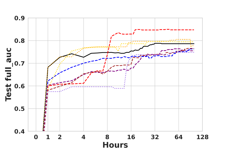
On AIROGS, we also track additional metrics recommended by the authors [22]: AUROC, partial AUROC (${>}$90% specificity) and sensitivity-at-95%-specificity.

Architectures. CNN-based models are popular in medical imaging [25, 66, 67, 28, 27, 5, 48, 26, 39]. We use ResNet-18 [33] on Tissue and PathMNIST, and Wide ResNet-28-2 [70] on TMED-2. We experiment with both ResNet-18 and 50 on AIROGS to assess architectural differences.

Training with early stopping. For each training phase, we perform minibatch gradient descent on Eq. (1) with Adam [45] optimizer and a cosine learning rate schedule [58]. Each training phase proceeds for up to 200 epochs, where one epoch represents enough minibatch updates to process the equivalent of the entire dataset $\mathcal{L}\bigcup\mathcal{U}$. After every epoch, we record balanced accuracy on the validation set. If this value plateaus for 20 consecutive epochs, we stop the current training phase early.

Hyperparameters. Semi- and self-supervised learning can both be sensitive to hyperparameters [60, 64]. Our evaluations tune both shared variables (e.g. learning rates, weight decay, unlabeled loss weight $\lambda^{U}$) as well as hyperparameters unique to each algorithm. See App. F.1 for details on all hyperparameters for all methods.

Unified procedure for training and hyperparameter tuning. We formulate a unified procedure mindful of realistic hardware and runtime constraints for a non-industrial-scale lab working on a new medical dataset. We assume each algorithm has access to one NVIDIA A100 GPU for a fixed number of hours. Within the alotted compute budget, for each algorithm we execute a serial random search over hyperparameters, sequentially sampling each new configuration and then training until the early stopping or maximum epoch is reached. We track the best-so-far classifier in terms of validation-set performance every epoch. Algorithm D.1 provides pseudocode for the procedure. Each time a new hyperparameter configuration is needed, we sample each hyperparameter value independently from a distribution designed to cover its common settings in prior literature (App. F.1). Our choice of random search on a budget is thought to yield better performance than grid search [3], fairly expends the same effort to train all methods regardless of their cost-per-epoch or hyperparameter complexity, and does not assume industrial-scale access to 1000 cloud-computing trials as in Oliver et al. [54]. As a rule of thumb, we find that performance saturates after about 25 hours per 80000 unlabeled examples. We thus allocate for the total time budget 25 hours for PathMNIST, 50 hours for TissueMNIST, and 100 hours for TMED-2. We allow 100 hours for AIROGS due to its larger resolution. Due to limited resources, we select only a few competitive methods to run on AIROGS based on the results on other datasets.

Self-supervised classification phase. Self-supervised methods by definition do not utilize label information when training representation layer weights $v$. To enable a proper comparison, for all self-SL methods our Alg. D.1 introduces an additional classification layer, training it anew after each epoch, each time using a 10 trial random search for an L2-penalty regularization hyperparameter. We retain the best performing weights $w$ on the validation set. We emphasize that $w$ does not impact overall self-supervised training of $v$.

Data augmentation. Following common practice, random flip and crop augmentations are used for all semi-supervised methods as well as Sup and MixUp. MixMatch also utilizes MixUp [74], while RandAugment [20] is used by FixMatch and FlexMatch. For each self-supervised method as well as SupCon, we apply the same SimCLR augmentation: random flip, crop, color jitter, and grayscale.

Multiple trials. We repeat Alg. D.1 for each method across 5 separate trials (distinct random seeds). We record the mean balanced accuracy on valid and test sets of these trials every 60 minutes (every 30 min. for Tissue and Path).

Figure 1: Balanced accuracy over time profiles of semi- and self-supervised methods across all 4 datasets. At each time, we report the test set bal. acc. of each method (mean over 5 trials of Alg. D.1). Best viewed electronically. Top Row: On these 3 datasets, we compare all 6 semi- and 7 self- methods (see legend in lower right, citations in Sec. 2), to 3 labeled-set-only baselines. Bottom Row: On larger AIROGS dataset, we compare selected methods representative of the best in the top row. Thin lines show final performance to ease comparison. From these charts, we suggest that our unified training and tuning (Alg. D.1) is effective, as all methods show gains over time.

6 RESULTS & ANALYSIS

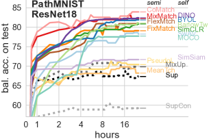
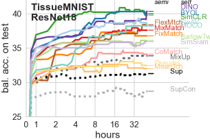
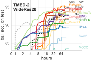
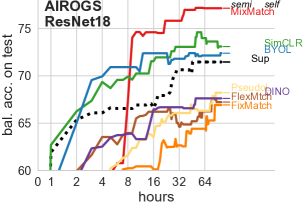
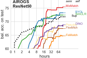
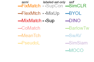
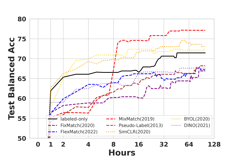
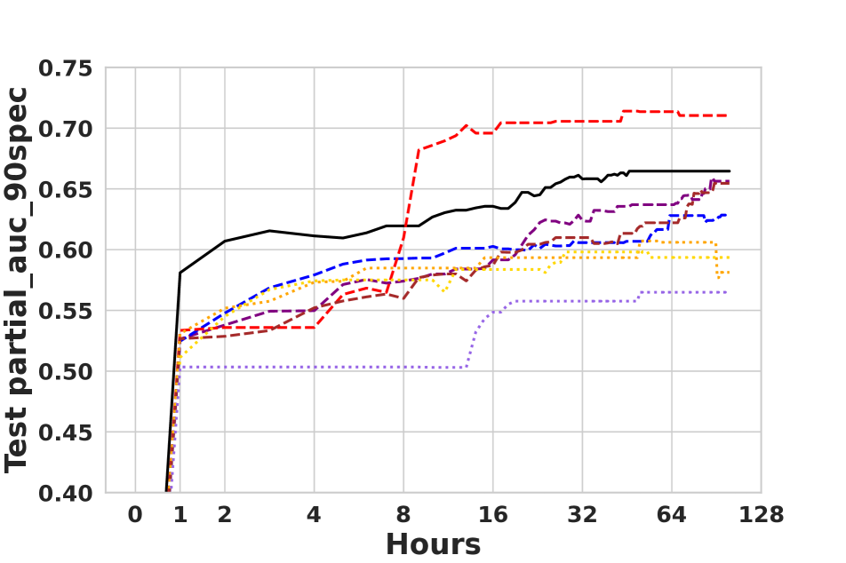
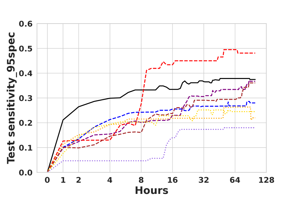
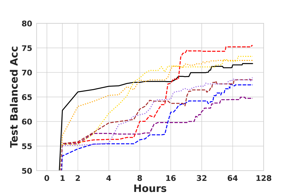
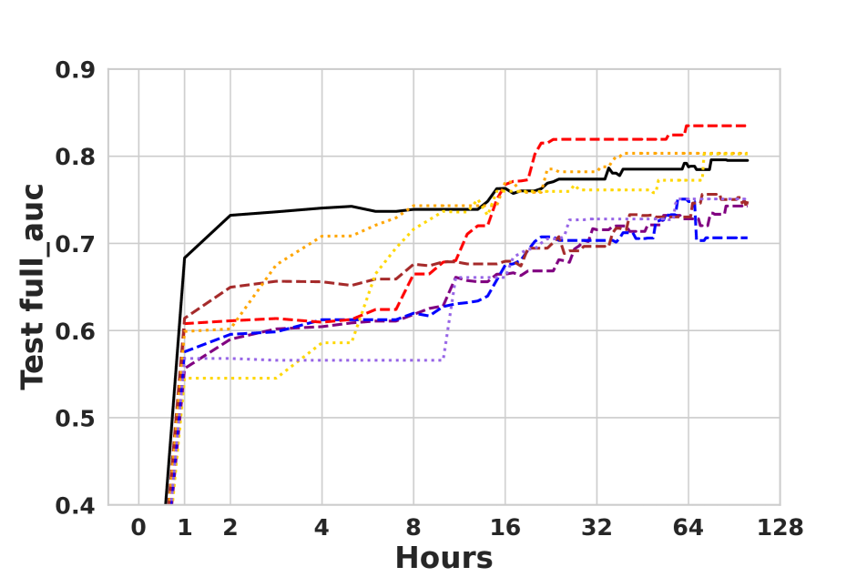
In each panel of Fig. 1, we focus on one dataset and architecture, plotting for each algorithm one line showing test set balanced accuracy (averaged across 5 trials) as a function of time spent running Alg. D.1. Variance across trials are presented in Fig C.4. Extra results on AIROGS showing other performance metrics over time (AUROC, partial AUROC and Sensitivity at 95% specificity) are found in Fig. C.3. We emphasize that following best practice, each checkpoint represents the best hyperparameters as selected on the validation set; we then just report that checkpoint’s test set performance. These results help us answer two key questions:

Is hyperparameter tuning worthwhile for SSL methods when validation set sizes cannot be larger than the train set? Across Fig. 1 and C.3, all 16 algorithms show roughly monotonic improvements in test performance over time, despite using a realistic-sized validation set. The final performance of every algorithm and dataset shows improvement due to our unified training and tuning procedure (further discussion in App. E.1.1). Therefore, we answer: Yes, realistically-sized validation sets for hyperparameter tuning and checkpoint selection can be effective.

What are the best SSL methods?. Among the many methods we study in Fig. 1, no method clearly outperforms others across all datasets. On Path, CoMatch, MixMatch, DINO, and BYOL perform best. On Tissue, self-supervised methods like DINO, BYOL, and SimCLR score well. On TMED-2, ultimately only FixMatch and MixMatch are competitive with the MixUp baseline. On AIROGS, only MixMatch, SimCLR and BYOL beat the Sup baseline.

Across all semi- and self- SSL methods, Tab. 3 reports the gain provided over the best labeled-set-only baseline. We conclude that MixMatch represents the best overall choice as it consistently performs at or near the top across all tasks, and is the only method to never deliver notably worse results than the best labeled-set-only baseline. However, hyperparameter tuning is necessary for MixMatch to succeed given a new dataset (see AIROGS result in Tab. 4).

	Gain in Bal. Acc. over best labeled-set-only
name	Path	Tissue	TMED	AIROGS	median	worst
MixMatch	12.4	3.7	-0.2	5.7	4.7	-0.2
MOCO	7.9	4.4	-11.3	n/a	4.4	-11.3
SwAV	8.4	4.3	-8.2	n/a	4.3	-8.2
SimCLR	11.0	5.9	-3.4	1.6	3.8	-3.4
BYOL	12.1	6.2	-5.6	0.9	3.5	-5.6
BarlowTw	11.2	2.2	-1.9	n/a	2.2	-1.9
DINO	12.6	6.5	-2.2	-3.8	2.2	-3.8
SimSiam	1.9	2.1	-12.9	n/a	1.9	-12.9
FlexMtch	11.1	4.5	-1.1	-4.2	1.7	-4.2
FixMatch	9.3	2.9	0.2	-4.5	1.6	-4.5
CoMatch	14.1	0.2	-3.0	n/a	0.2	-3.0
MeanTch	-1.6	-1.9	-1.2	n/a	-1.6	-1.9
PseudoL	0.6	-1.4	-4.4	-3.2	-2.3	-4.4
ref acc.	69.8	33.9	94.9	71.5

Table 3: Gains from SSL methods over only using labeled set, across 4 datasets. Self (italicized), Semi (normal). We report gains in percentage balanced accuracy (higher is better) in the mean final test set performance (averaged over 5 runs of Alg. D.1) over a reference value that represents the best labeled-set-only run among Sup (minimize cross entropy), SupCon, and MixUp. MixMatch has the highest median gain, and is the only method to never score notably worse ($>$ 1 point) than the best labeled set only run.

Pretraining vs. from scratch. Plots in App. C show accuracy-over-time profiles using initial weights pretrained on ImageNet. Compared to training from scratch, we do not see notable gains in ultimate test-set accuracy when top methods use pretrained weights. With this in mind, pretraining’s benefits still include improved convergence speed and reduced variance across trials.

ResNet-18 vs. ResNet-50. The bottom row of Fig 1 compares ResNet-18 and ResNet-50 architectures on AIROGS. We broadly find that the method rankings are similar. More notably, ResNet-50 is not substantially better than ResNet-18 in this task when compared using the same runtime budget. Profiles of other performance metrics in App C.3 suggest the same conclusions.

Tuning vs. Transfer Hypers from another Dataset. To make the most of limited labeled data, one potential strategy is to use the entire labeled set for training, reserving no validation set at all. This approach relies on pre-established “best” hyperparameters sourced from other datasets, obviating the need for data-specific hyperparameter tuning. Su et al. [60] employed this strategy in their benchmark, suggesting tuning on small-validation sets would likely yield unreliable or suboptimal accuracy. However, this claim was not supported by any direct experimental comparison in their work. Here in Tab. 4, we directly compare our hyperparameter tuning strategy (Alg. D.1) with Su et al.’s transfer strategy. We train the latter on the combined train + validation sets (100 epochs on PathMNIST and AIROGS, and 80 epochs on TMED2). Training is terminated early if the train loss does not improve over 20 consecutive epochs (full details in App. D.2). Empirically, we observe that all models which did not trigger early stopping reached a plateau in training loss. We report the final test-set balanced accuracy of each strategy on the PathMNIST, TMED-2 and AIROGS.

		PathMNIST				TMED-2				AIROGS
Hyperparam. strategy:		Search	Best from	Best from		Search	Best from	Best from		Search	Best from	Best from
			Tissue	CIFAR-10			Tissue	CIFAR-10			Tissue	CIFAR-10
semi	MixMatch	82.24	83.87	73.51		94.71	92.67	74.73		77.14	61.75	Diverged
	CoMatch	83.95	80.51	86.42		91.87	92.51	92.67
	FixMatch	79.11	82.64	79.73		95.06	95.12	95.73		66.92	66.31	65.50
	FlexMatch	80.91	78.70	80.23		93.77	93.97	93.70		67.23	72.82	74.52
	Pseudo-Label	70.42	66.12	64.71		90.52	88.78	82.13		68.21	64.43	66.93
	Mean-Teacher	68.21	55.90	56.13		93.70	91.21	58.26
self	SimCLR	81.05	79.86	80.05		91.50	86.37	91.17		73.01	67.15	67.95
	BYOL	81.79	80.35	80.16		89.26	90.65	89.08		72.40	70.13	70.63
	SwAV	77.90	78.24	81.30		86.72	81.23	83.19
	MoCo	77.73	79.95	79.12		83.55	81.15	80.23
	SimSiam	71.78	68.62	70.44		81.97	79.05	82.16
	BT	80.85	72.79	80.25		92.98	92.52	88.48
	DINO	82.52	77.50	80.67		92.71	92.02	94.28		67.61	66.46	67.13

Table 4: Hyperparameter strategy evaluation. Table reports ultimate test-set balanced accuracy as percentage (mean over 5 trials, higher is better) on three target datasets: PathMNIST, TMED-2, and AIROGS. 3 different hyperparameter strategies are compared for each SSL method. Note that due to computation constraints, we only select a few algorithms to run on AIROGS, explained in Sec 5. Search strategy: tuning for best hyperparameters via our proposed Alg. D.1 for 100 (TMED-2 and AIROGS) and 25 hours (PathMNIST), using provided train/validation split. Best from Tissue/CIFAR-10 strategy: just one training phase on the target dataset using the “best” hyperparameters selected from the named source data. These runs combine train and validation data for fitting following Su et al. [60], and typically take 1-4/5-30/10-40 hours on Path/TMED-2/AIROGS depending on the algorithm and whether early stopping is triggered. To highlight which strategies are most effective, we bold the best strategy within each dataset-specific row, and color cells relative to this bold value as green (within 2.5 of best), yellow (within 5 of best), and red (worse by 5 or more points).

From Tab. 4, we see that our hyperparameter search is competitive across all datasets. (see all the green cells under “Search”). However, it does require the greatest runtime. On the other hand, transferring hyperparameters from another dataset without the use of a validation set may occasionally yield reasonable results. However, there is no guarantee of good performance, as evidenced by the inferior cases highlighted in yellow and red. Additionally, there is no consistent distinction between transferring from Tissue (arguably a more related medical dataset) and transferring from CIFAR10, underscoring the challenge of identifying a “closely related” dataset for hyperparameter transfer.

Overall, we recommend researchers with a new task at hand should adopt our hyperparameter tuning strategy. Using all data for training (reserving no validation set) by adopting off-the-shelf hyperparameter does not necessarily guarantee good performance. Even with somewhat compatible off-the-shelf hyperparameter, no validation set makes checkpoint selection challenging. Adjacent epochs that exhibit similar low training losses may differ by over 5% in test accuracy in our experiments. How to tranfer from existing hyperparameter to new task is an interesting further direction of research.

7 DISCUSSION & CONCLUSION

We have contributed a benchmark that helps practioners quantify what gains in a classification task are possible from the addition of unlabeled data and which methods help achieve them. We offer a unified approach to training and hyperparameter selection of semi-supervised methods, self-supervised methods, and supervised baselines that is both affordable and realistic for research labs tackling new challenges without industrial-scale resources.

Limitations. Use caution when extrapolating our findings beyond the dataset sizes, modalities, resolutions and class compositions studied here. We deliberately focused on a modest number of labeled examples (30 - 1000) per class, motivated by projects where substantive effort has already gone into labeled data collection. Applications in more scarce-label regimes (e.g. zero-shot or few-shot methods) may need to also consult other benchmarks, as should those looking at hundreds of fine-grained classes.

To enable thorough experiments, we focused on moderate ResNet architectures that have proven effective in clinical applications [66, 67]. It would be valuable to understand if similar findings hold with vision transformer architectures, though we leave this to future work due to the substantial effort required. Additionally, our results would ideally be verified across multiple train-validation splits; however the resources needed remain prohibitive.

Even for the datasets and architectures we study, our analysis here is limited to understanding the performance-over-time of balanced accuracy and sensitivity-specificity metrics (for AIROGS). Other clinically useful metrics, such as AUPRC, calibration or net benefit, are often needed to decide if a classifier is appropriate for deployment [59]. For medical applications, it is also key to understand fairness of methods across subpopulations [12] to avoid propagating structural disadvantages.

Broader impact. All data analyzed here represent fully-deidentified open-access images approved for widespread use by their creators. We think the benefit of promoting these medical tasks to advance ML research outweighs the slight risk of patient reidentification by a bad actor.

Outlook. Our experiments show that real benefits from the addition of unlabeled data are sometimes possible: our recommended methods see gains of +5 points of balanced accuracy on TissueMNIST, +10 points on PathMNIST, and +5 points on AIROGS against strong labeled-set-only baselines. In contrast, most tested methods do not add significant gains on TMED-2, perhaps due to that benchmark’s uncurated nature [38]. We hope our code release enables the medical research community to convert decades of effort on SSL into improved patient outcomes and better scientific understanding of disease and possible treatments. We further hope that our benchmark inspires those that pursue improved methodological contributions to favor realistic evaluation protocols.

[sections]

Appendix Contents

[sections]l1

Appendix A Code and Data Splits for Reproducibility

All code resources needed to reproduce our analysis can be found in our github repo

https://github.com/tufts-ml/SSL-vs-SSL-benchmark

The exact splits of the TissueMNIST, PathMNIST, TMED-2, AIROGS we used will also be provided upon acceptance.

Our codebase builds upon the open-source PyTorch repo by Suzuki [61]. We added many additional algorithms (we added MixMatch, FixMatch, FlexMatch, and CoMatch, as well as all 7 self-supervised methods) and customized the experiments, especially providing a runtime-budgeted hyperparameter tuning strategy as outlined in App. D.

Suzuki’s code was intended as a reimplementation in PyTorch of Oliver et al. [54]’s benchmark of semi-supervised learning (while Oliver et al’s original repo was in Tensorflow, we prefer PyTorch).

In a way, this makes our repo a “cousin” of the codebase of Su et al. [60]’s fine-grained classification benchmark, because their github repo also credits Suzuki’s repo as an ancestor.

Appendix B Dataset Details

B.1 Dataset Selection

We selected PathMNIST and TissueMNIST from 12 candidate datasets in the MedMNIST collections [68, 69] by matching two criteria: (i) contains at least 5 imbalanced classes; (ii) can build a large unlabeled set (at least 50000 images). Prior experiments from dataset creator Yang et al. [69] suggest 28x28 resolution is a reasonable choice. They report that a larger resolution (224x224) does not yield much more accurate classifiers for these two datasets.

B.2 Class Description

TissueMNIST contains images of human kidney cortex cells. The dataset contains 8 classes. See  [69] for more details.

Class ID	Abbreviation	Description
0	CD/CT	Collecting Duct, Connecting Tubule
1	DCT	Distal Convoluted Tubule
2	GE	Glomerular endothelial cells
3	IE	Interstitial endothelial cells
4	LEU	Leukocytes
5	POD	Podocytes
6	PT	Proximal Tubule Segments
7	TAL	Thick Ascending Limb

PathMNIST contains patches from colorectal cancer histology slides that comprise of 9 tissue types. See [69, 42] for more details.

Class ID	Abbreviation	Description
0	ADI	adipose
1	BACK	background
2	DEB	debris
3	LYM	lymphocytes
4	MUC	mucus
5	MUS	smooth muscle
6	NORM	normal colon mucosa
7	STR	cancer-associated stroma
8	TUM	colorectal adenocarcinoma epithelium

TMED-2 contains 2D grayscale images captured from routine echocardiogram scans. In this study, we adopt the view classification task from  [36]. For more detail please see [36, 37]

Class ID	Abbreviation	Description
0	PLAX	parasternal long axis
1	PSAX	parasternal short axis
2	A2C	apical 2-chamber
3	A4C	apical 4-chamber

AIROGS is a dataset of color image of the retina. The binary classification task is to differentiate between referable glaucoma and no referable glaucoma [22].

Class ID	Abbreviation	Description
0	No Glauc.	no referable glaucoma
1	Glaucoma	referable glaucoma

Appendix C Additional Results

C.1 Impact of pretraining on accuracy-over-time profiles

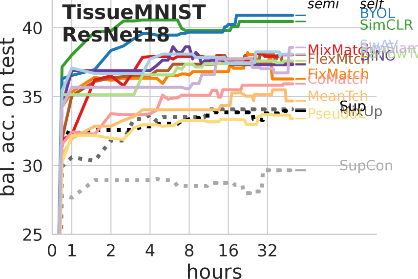
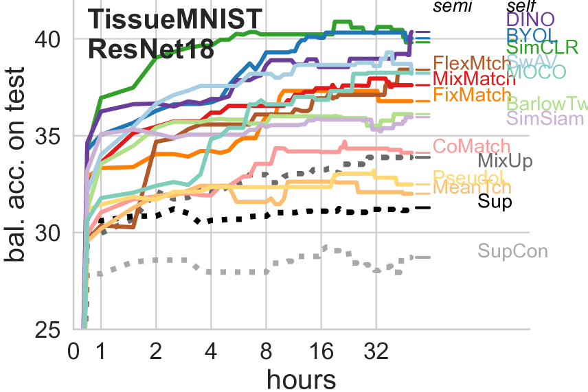
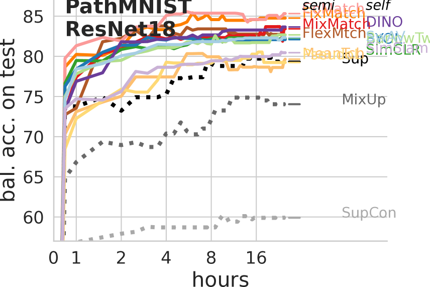
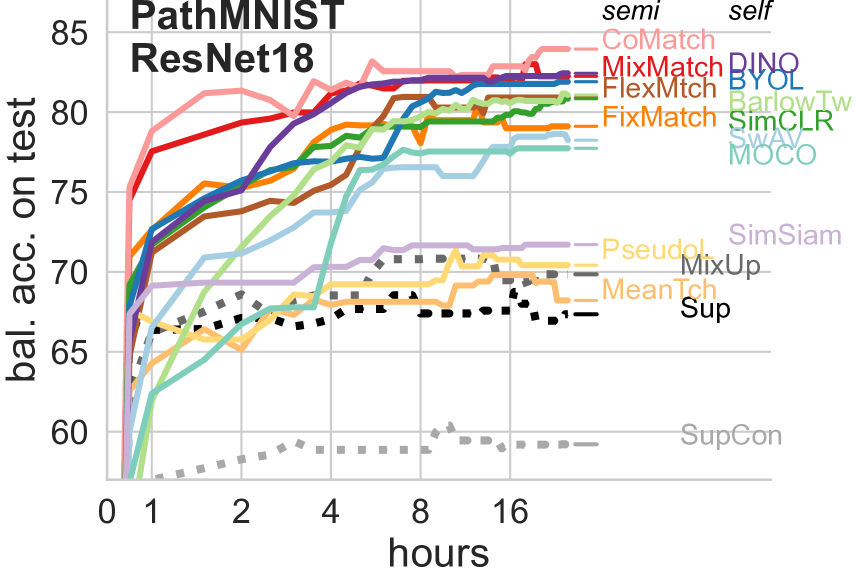
To study the impact of pretraining, we compare the accuracy-over-time profiles of TissueMNIST and PathMNIST based on the two different initialization strategy.

Fig. C.1 left column shows pretraining on ImageNet strategy, right column shows random initialization. On TissueMNIST, SimCLR (green) and BYOL (blue) are the top two methods in both cases. On PathMNIST, semi-supervised methods seem better: FixMatch and CoMatch are best on the pretraining case, with MixMatch and Flexmatch only a few points of balanced accuracy lower. MixMatch and CoMatch are best in the random initialization case.

Across both plots, pretraining does not seem to impact the top-performing methods’ ultimate accuracy by much. (e.g. by more than a few points of accuracy). However, with more limited time budgets (e.g. after only a few hours), we do see initialization from pretraining understandably tends to improve some methods. Pretraining time on a source dataset is NOT counted to the runtime reported in x-axis.

(a) TissueMNIST : pretrained initial weights

(b) TissueMNIST : random initial weights

(c) PathMNIST : pretrained initial weights

(d) PathMNIST: random initial weights

Figure C.1: Balanced accuracy on test set over time for semi- and self-supervised methods, with (left) and without (right) initial weight pretraining on ImageNet. Curves represent mean of each method at each time over 5 trials of Alg.  D.1.

C.2 Comparing validation profiles of accuracy-over-time

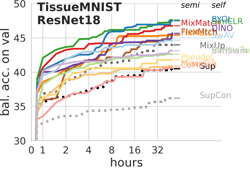
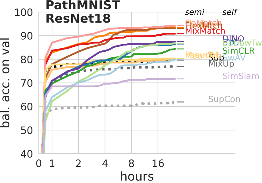
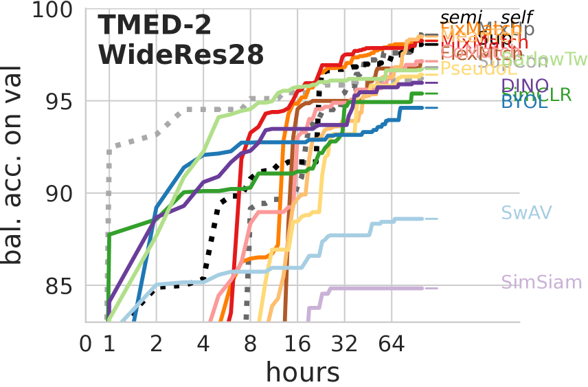
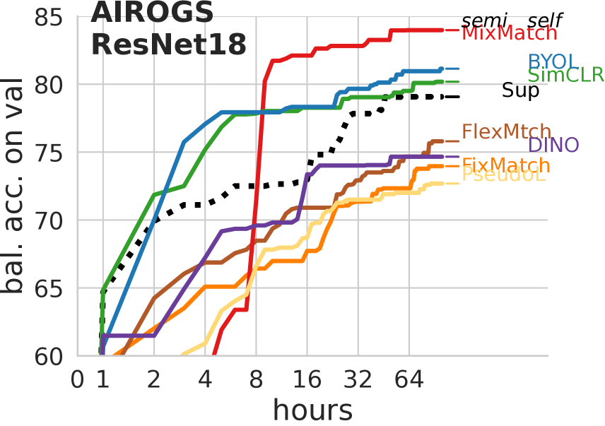
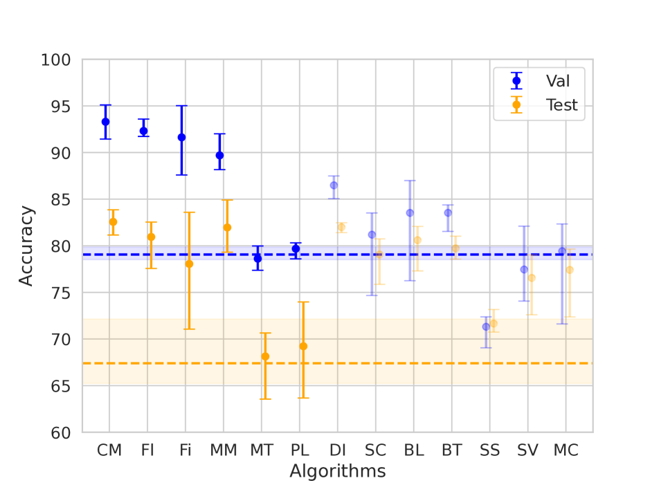
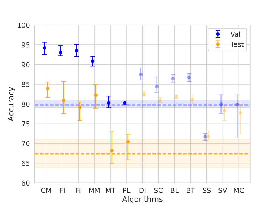
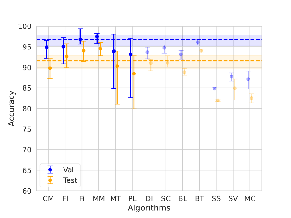
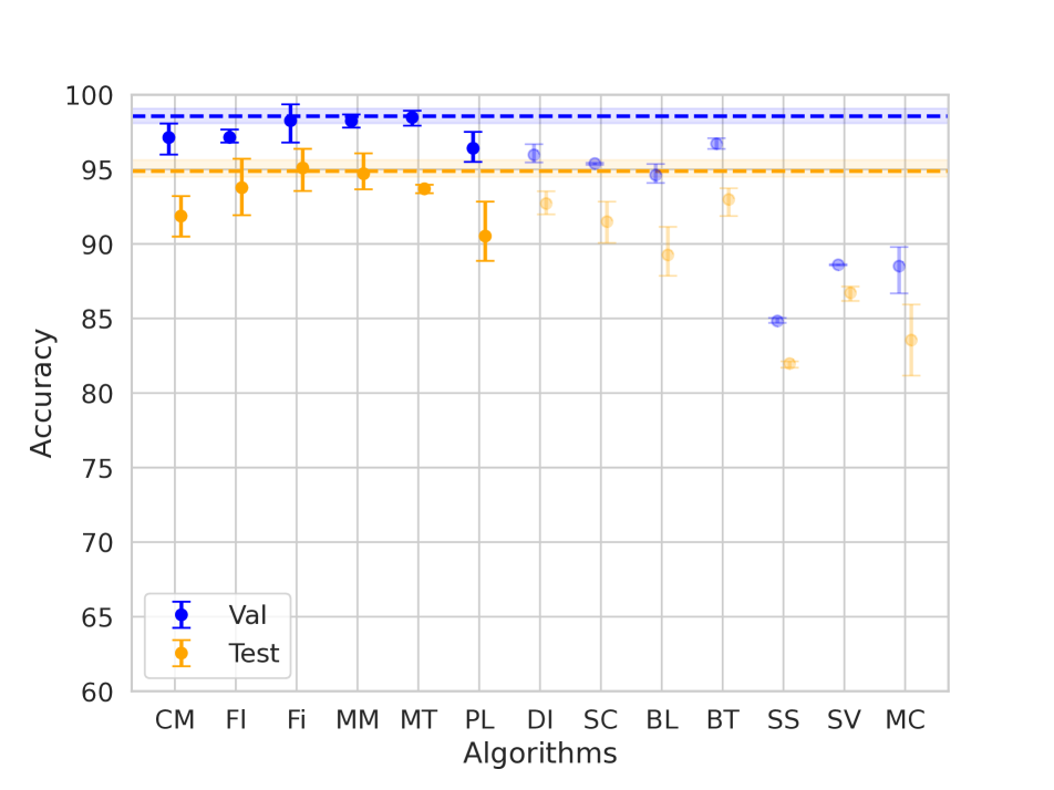
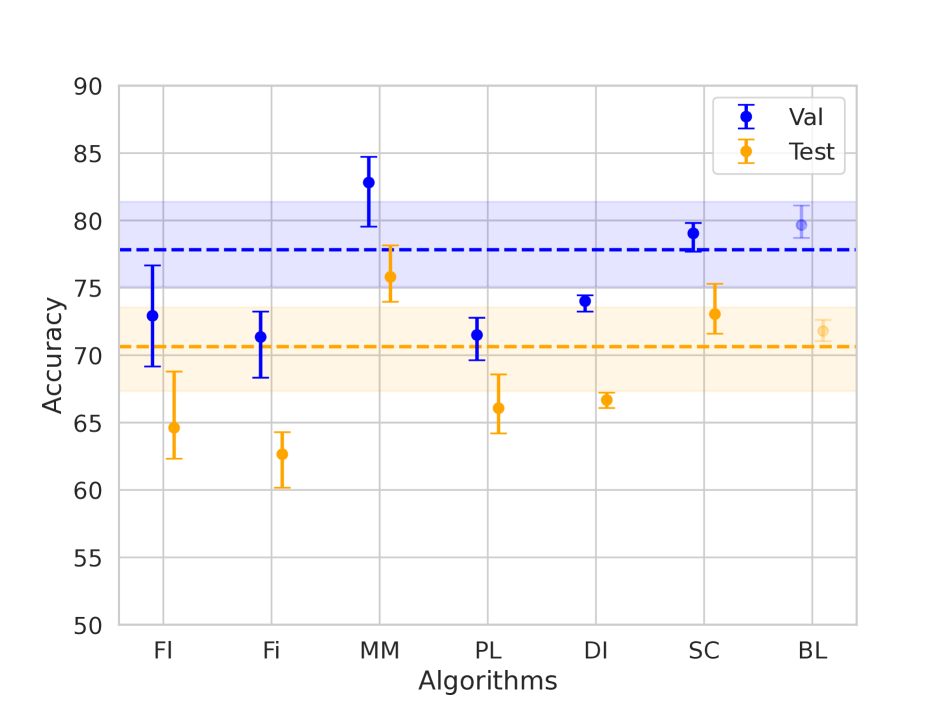
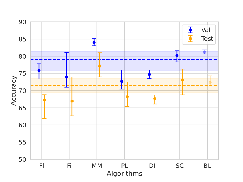
Fig. C.2 shows profiles of accuracy over time on the validation set, in contrast to the test set performance shown in the main paper’s Fig. 1.

All curves here by definition must be monotonically increasing, because our unified algorithm selects new checkpoints only when they improve the validation-set balanced accuracy metric. The important insight our work reveals is that the same model checkpoints selected here, based on validation-set accuracy, also tend to produce improved test-set accuracy over time (in Fig. 1). This helps provide empirical confidence in using realistically-sized validation sets.

(a) TissueMNIST

(b) PathMNIST

(c) TMED2

(d) AIROGS

Figure C.2: VALIDATION accuracy over time profiles of semi- and self-supervised methods on 4 datasets (panels a-d).All curves here by definition must be monotonically increasing. We see that the increasing validation set performance translate to increasing test set performance in Fig. 1.

C.3 Additional Evaluation Metrics

(a) Balanced Acc

(b) full auc

(c) Partial AUC

(d) Sensitivity

(e) Balanced Acc

(f) full auc

(g) Partial AUC

(h) Sensitivity

Figure C.3: Upper: Res18. Lower: Res50. The figure from left to right are Test Performance over time profiles of semi- and self-supervised methods on AIROGS dataset across 4 metircs: Balanced Accuracy, AUC, Partial AUC for 90% - 100% specificity and Sensitivity at 95% specificity (panels a-c). At each time, we report mean of each method over 5 trials of Alg. D.1.

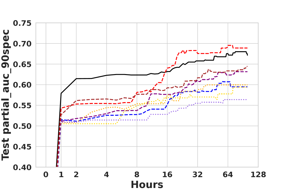
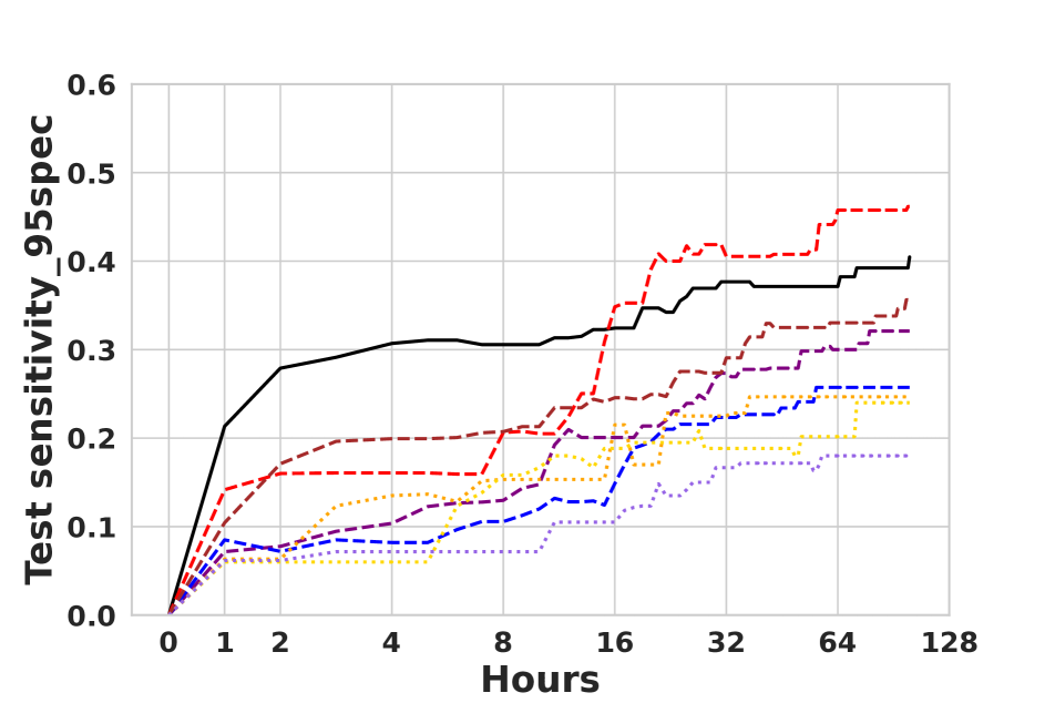
C.4 Variance Across Trials

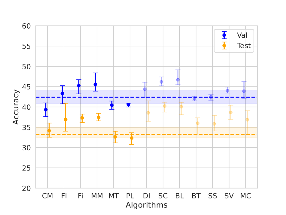
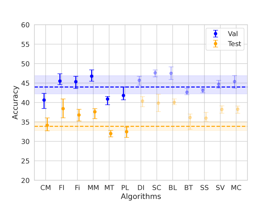
In Fig. C.4 below, we explicitly visualize the variability in performance of each method across the 5 separate trials of Alg. D.1 (most other figures show the mean of these 5 trials for visual clarity).

(a) TissueMNIST after 16h

(b) TissueMNIST after 50h

(c) PathMNIST after 8h

(d) PathMNIST after 25h

(e) TMED-2 after 32h

(f) TMED-2 after 100h

(g) AIROGS(res18) after 32h

(h) AIROGS(res18) after 100h

Figure C.4: Balanced accuracy of different methods across 2 time budgets (columns) and four datasets (rows). For each method, the interval indicates the low and high performance of 5 separate trials of Alg. D.1, while dot indicates the mean performance. Horizontal lines indicate the best labeled-set-only baseline at that time. Abbreviation: CM, Fl, Fi, MM, MT, PL, DI, SC, BL, BT, SS, SV, MC denote CoMatch, FlexMatch, FixMatch, MixMatch, Mean Teacher, Pseudo Label, DINO, SimCLR, BYOL, Barlow Twins, SimSiam, SwAV, MOCO (v2).

Appendix D Algorithms Details

D.1 Algorithm : Random Hyperparameter search on a budget

Algorithm D.1 outlines our uniform hyperparameter tuning procedures used across all algorithms under comparison. The algorithm requires three sources of data: a labeled training set $\mathcal{L}=\{X,Y\}$, an unlabeled set for training $\mathcal{U}=X^{U}$, and a separate realistically-sized labeled validation set $\{X^{val},Y^{val}\}$. We further require some budget restrictions: a common computational budget $T$ (maximum number of hours), and a maximum training epoch per hyperparameter configuration $E$.

We proceed as follows: We begin by randomly sampling a hyperparameter configuration from a defined range (see Appendix F.1 for details). A model is then initialized and trained using the ADAM optimizer with the sampled hyperparameters. Each configuration is trained for a maximum of $E$ (200) epochs or stopped early if the validation performance does not improve for 20 consecutive epochs. The model’s performance on the validation set is measured using balanced accuracy. Upon completion of training for a given hyperparameter configuration (either after reaching maximum epoch $E$ or after early stopping), a new configuration is sampled and the process repeats until the total compute budget $T$ is expended.

We track the best-so-far model performance every 30 minutes, and save the best-so-far model and its corresponding validation and test performance. Semi-supervised algorithms simultaneously train the representation layers $v$ and classifier layer $w$, while self-supervised algorithms train the representation layers $v$ for each epoch and then fine-tune a linear classifier with weights $w$ anew at the end of each epoch using sklearn logistic regression model [56] with representation parameters $v$ frozen.

Algorithm D.1 Unified Procedure for Training + Hyperparameter selection via random search

Input:

• Train set of features $\mathbf{X}$ paired with labels $\mathbf{Y}$, with extra unlabeled features $\mathbf{U}$

• Validation set of features $\mathbf{X}^{\text{val}}$ and labels $\mathbf{Y}^{\text{val}}$

• Runtime budget $T$, Max Epoch $E$

Output: Trained weights $\{v,w\}$, where $v$ is the representation module, $w$ is the classifier layer

1:while time elapsed $<$ T do

2:     $\lambda\sim\textsc{DrawHypers}$ $\triangleright$ Sample hyperparameters for pre-defined range

3:     $\xi\leftarrow\textsc{CreateOptim}(\lambda)$ $\triangleright$ Initialize stateful optimizer e.g., ADAM

4:     $\{v,w\}\sim\textsc{InitWeights}$ $\triangleright$ Initialize model weights

5:     for epoch $e$ in $1,2,\ldots,E$ do

6:         if self-supervised then

7:              $v\leftarrow\textsc{TrainOneEpoch}(\mathbf{U},v,\lambda,\xi)$ $\triangleright$ Optimize Eq. with $\lambda^{L}=0$

8:              $w\leftarrow\textsc{TrainClassifier}(\mathbf{Y},f_{v}(\mathbf{X}))$

9:         else if semi-supervised then

10:              $v,w\leftarrow\textsc{TrainOneEpoch}(\mathbf{X},\mathbf{Y},\mathbf{U},v,w,\lambda,\xi)$ $\triangleright$ Optimize Eq.

11:         else

12:              $v,w\leftarrow\textsc{TrainOneEpoch}(\mathbf{X},\mathbf{Y},v,w,\lambda,\xi)$ $\triangleright$ Optimize Eq. with $\lambda^{U}=0$

13:         end if

14:         $m_{e}\leftarrow\textsc{CalcBalAcc}(\mathbf{X}^{\text{val}},\mathbf{Y}^{\text{val}},v,w)$ $\triangleright$ Record performance metric on val.

15:         if first try or $m_{e}>m_{*}$ then

16:              $v_{*},w_{*}\leftarrow v,w$; $\lambda_{*}\leftarrow\lambda$; $m_{*}\leftarrow m_{e}$ $\triangleright$ Update best config found so far

17:         end if

18:         if EarlyStop($m_{1},m_{2},\ldots,m_{e}$) or time elapsed $>T$ then

19:              break

20:         end if

21:     end for

22:end while

23:return $v_{*},w_{*},\lambda_{*},m_{*}$

D.2 Hyperparameter transfer strategy

To make the most of limited labeled data, one potential strategy is to use the entire labeled set for training, reserving no validation set at all, and thus relies on pre-established hyperparameters from other dataset/experiments. In this study, we experiment with two scenarios: using pre-determined hyperparameters from 1. CIFAR-10, or 2. TissueMNIST. The CIFAR-10 hyperparameters are sourced from public repositories, we ensure that our CIFAR-10 hyperparameter choices on our re-implementation of the algorithms matches previously reported results in the literature. The TissueMNIST hyperparameters originate from our experiments as depicted in Figure C.2 ($a$).

D.3 Semi-supervised method details.

Semi-supervised learning trains on the labeled and unlabeled data simultaneously, usually with the total loss being a weighted sum of a labeled loss term and an unlabeled loss term. Different methods mainly differs in how unlabeled data is used to form training signals. Many approaches have been proposed and refined over the past decades. These include co-training, which involves training multiple classifiers on various views of the input data [6, 53]; graph-structure-based models [76, 40]; generative models [46, 47]; consistency regularization-based models that enforce consistent model outputs [49, 62, 4]; pseudo label-based models that impute labels for unlabeled data  [50, 11]; and hybrid models that combines several methods [58]. Comprehensive reviews can be found in Zhu [77], Chapelle et al. [13], Van Engelen and Hoos [63].

Among the deep classifier methods following Eq. (1), below we describe each method we selected and how its specific unlabeled loss is constructed.

Pseudo-Labeling

uses the current model to assign class probabilities to each sample in the unlabeled batch. If, for an unlabeled sample, the maximum class probability $P(y_{i})$ exceeds a certain threshold $\tau$, this sample contributes to the calculation of the unlabeled loss for the current batch. The cross-entropy loss is computed as if the true label of this sample is class $i$.

Mean-Teacher

constructs the unlabeled loss by enforcing consistency between the model’s output for a given sample and the output of the same sample from the Exponential Moving Average (EMA) model.

MixMatch

uses the MixUp [74] technique on both labeled data (features and labels) and unlabeled data (features and guessed labels) within each batch to produce transformed labeled and unlabeled data. The labeled and unlabeled losses are then calculated using these transformed samples. Specifically, the unlabeled loss is derived from the mean squared error between the model’s output for the transformed unlabeled samples and their corresponding transformed guessed labels.

FixMatch

generates two augmentation of an unlabeled sample, one with weak augmentation and the other using strong augmentations (e.g., RandAug [20]). The unlabeled loss is then formulated by enforcing the model’s output for the strongly augmented sample to closely resemble that of the weakly augmented sample using cross-entropy loss.

FlexMatch

builds directly upon FixMatch by incorporating a class-specific threshold on the unlabeled samples during training.

CoMatch

marks the first introduction of contrastive learning into semi-supervised learning. The model is equipped with two distinct heads: a classification head, which outputs class probabilities for a given sample, and a projection head, which maps the sample into a low-dimensional embedding. These two components interact in a unique manner. The projection head-derived embeddings inform the similarities between different samples, which are then used to refine the pseudo-labels against which the classification head is trained. Subsequently, these pseudo-labels constitute a pseudo-label graph that trains the embedding graph produced by the projection head.

D.4 Self-supervised method details

In recent years, self-supervised learning algorithms have emerged rapidly and are known as one of the most popular field of machine learning. These include contrastive learning, which involves learning representations by maximizing agreement between differently augmented views of the same data [15, 34]; predictive models that forecast future instances in the data sequence [55]; generative models that learn to generate new data similar to the input [14]; clustering-based approaches that learn representations by grouping similar instances [8, 9]; context-based models that predict a specific part of the data from other parts [23, 7]; and hybrid models that combine various methods for more robust learning [16]. A more comprehensive review can be found in [41, 78].

Below, we provide for each selected self-supervised method a summary of its internal workings.

SimCLR

generates two augmented versions of each image. Then feed these pairs of images into a base encoder network to generate image embeddings. This encoder is followed by a projection head, which is a multilayer neural network, to map these embeddings to a space where contrastive loss can be applied. Next, calculate the contrastive loss. The idea is to make the embeddings of augmented versions of the same image (positive pairs) as similar as possible and to push apart embeddings from different images (negative pairs). The loss function used is NCE loss.

MOCO V2

creates two augmented versions of each image. These pairs are processed by two encoder networks: a query encoder, and a key encoder updated by a moving average of the query encoder. The contrastive loss is computed by comparing a positive pair (the query and corresponding key) against numerous negative pairs drawn from a large queue of keys.

Note on runtime: We notice that the performance on MoCo can be increased when Shuffling BN across multiple GPUs. However, to ensure a fair comparison given our single-GPU setup, we refrained from employing any techniques to simulate multiple GPUs on one, as this would change the encoder’s structure.

SwAV

begins by creating multiple augmented versions of each image. Then, these versions are input into a deep neural network to generate embeddings. Uses a clustering approach, called online stratified sampling, to predict assignments of each view’s prototypes (or cluster centers) to others, encouraging the model to match the representations of different augmentations of the same image.

Note on runtime: We’ve observed that applying multiple augmentations can enhance the effectiveness of various methods. To prevent the results from being influenced by these augmentations, we’ve standardized the number of augmentations to two in SwAV, in line with the approach taken by other methods.

BYOL

starts by creating two differently augmented versions of each image. These versions are processed through two identical neural networks, known as the target and online networks, which include a backbone and a projection head. The online network is updated through backpropagation, while the target network’s weights are updated as a moving average of the online network’s weights. The unique aspect of BYOL is that it learns representations without the need for negative samples.

SimSiam

creates two differently augmented versions of each image. These versions are passed through two identical networks: one predictor network and one encoder network. The encoder network contains a backbone and a projection head.

DINO

utilizes two differently augmented images, processed by a student and a teacher network. The teacher’s weights evolve as a moving average of the student’s. The key idea is self-distillation, where the student’s outputs match the teacher’s for one view but differ for the other, without traditional negative samples.

Barlow Twins

processes two augmented views of an image through identical networks. The aim is to have similar representations between these networks while minimizing redundancy in their components, sidestepping the need for contrasting positive and negative pairs.

Appendix E Additional Analysis

E.1 Hyperparameter Tuning and Model selection with realistic validation set

E.1.1 Effectivness of Hyperparameter Tuning

While Oliver et al. [54] caution that extensive hyperparameter search may be futile with realistic validation set. Our experiments on the 4 dataset show that the validation set performance for each examined algorithm rise substantially over the course of hyperparameter tuning. This increase in validation set performance further translates to increased test set performance.

This means that for a chosen algorithm on a new dataset, following our hyperparameter tuning protocol (even with limited labeling budget and computation budget), we can obtain better generalization (measured by test set performance).

E.1.2 Differentiating Between Models

Oliver et al. [54] in their Fig 5 and 6 show that on SVHN, between 10 random samples of the validation set across several level of validation set size (1000, 500, 250, 100), the validation accuracy of the trained Pi-model, VAT, Pseudo-labeling and Mean Teacher model has substantial variability and overlap with each other. Thus, they caution that differentiating between models might be infeasible with realistic validation set size.

In this study, we employ a relaxed notion of “realistic validation set”, by letting the validation set to be at most as large as the training set. Our experiments cover validation set size 235 (TMED), 400 (Tissue), 450 (Path), 600 (AIROGS); test set size 2019 (TMED2), 47280 (Tissue), 7180 (Path), 6000 (AIROGS). Our experiment shows that within the wide range of methods considered, differentiating between some models are possible. For example, we can see that MixMatch is clearly better than Mean Teacher in TissueMNIST and PathMNIST, in both the validation set and test set, without overlap on the intervals. The field of semi-supervised learning has made significant advancements in recent years. It is crucial to reevaluate previous conclusions in light of the new developments.

E.1.3 Theoretical Analysis

Here, we show that the performance gain we observe on the test set are real. We perform the same theoretical analysis using the Hoeffding’s inequality Hoeffding [35] as in Oliver et al. [54].

$$\mathbf{P}(|\bar{V}-\mathbb{E}[V]|<p)>1-2\exp(-2np^{2})$$ (3)

where $\bar{V}$ is the empirical estimate of some model performance metric, $\mathbb{E}[V]$ is its hypothetical true value, $p$ is the desired maximum deviation between our estimate and the true value, and $n$ is the number of examples used.

On TissueMNIST, we have 47280 test samples, we will be more than 99.98% confident that the test accuracy is within 1% of its true value. On Path, we have 7180 test samples, we will be more than 99% confident that the test accuracy is within 2% its true value.

In Fig 1, we see that after hyperparameter tuning, the final test accuracy of each algorithms improves much more than 1% on TissueMNIST and 2% on PathMNIST showing the efficacy of hyperparameter tuning.

Similarly, we can see that the difference between top-performing algorithms (e.g., MixMatch) and worst-performaning alogrithm (e.g., Mean Teacher) is clearly larger then 1% on TissueMNIST, 2% on PathMNIST. Thus we can argue that differentiation between certain methods are viable. Same analysis can also be applied to TMED-2 and AIROGS.

Appendix F Hyperparameter Details

F.1 Search Range

Below we show the search range of each hyperparameter.

.

Shared By All
Optimizer	Adam
Learning rate schedule	Cosine

Labeled only
Batch size	64
Learning rate	$3\times 10^{x},X\sim\text{Uniform}(-5,-2)$
Weight decay	$4\times 10^{x},X\sim\text{Uniform}(-6,-3)$

MixUp
Batch size	64
Learning rate	$3\times 10^{x},X\sim\text{Uniform}(-5,-2)$
Weight decay	$4\times 10^{x},X\sim\text{Uniform}(-6,-3)$
Beta shape $\alpha$	$x,X\sim\text{Uniform}(0.1,10)$

Sup Contrast
Batch size	256
Learning rate	$3\times 10^{x},X\sim\text{Uniform}(-5.5,-1.5)$
Weight decay	$4\times 10^{x},X\sim\text{Uniform}(-7.5,-3.5)$
Temperature	$x,X\sim\text{Uniform}(0.05,0.15)$

FlexMatch
Labeled batch size	64
Unlabeled batch size	448
Learning rate	$3\times 10^{x},X\sim\text{Uniform}(-5,-2)$
Weight decay	$4\times 10^{x},X\sim\text{Uniform}(-6,-3)$
Unlabeled loss coefficient	$10^{x},X\sim\text{Uniform}(-1,1)$
Unlabeled loss warmup schedule	No warmup
Pseudo-label threshold	0.95
Sharpening temperature	1.0

FixMatch
Labeled batch size	64
Unlabeled batch size	448
Learning rate	$3\times 10^{x},X\sim\text{Uniform}(-5,-2)$
Weight decay	$4\times 10^{x},X\sim\text{Uniform}(-6,-3)$
Unlabeled loss coefficient	$10^{x},X\sim\text{Uniform}(-1,1)$
Unlabeled loss warmup schedule	No warmup
Pseudo-label threshold	0.95
Sharpening temperature	1.0

CoMatch
Labeled batch size	64
Unlabeled batch size	448
Learning rate	$3\times 10^{x},X\sim\text{Uniform}(-5,-2)$
Weight decay	$4\times 10^{x},X\sim\text{Uniform}(-6,-3)$
Unlabeled loss coefficient	$10^{x},X\sim\text{Uniform}(-1,1)$
Unlabeled loss warmup schedule	No warmup
Contrastive loss coefficient	$5\times 10^{x},X\sim\text{Uniform}(-1,1)$
Pseudo-label threshold	0.95
Sharpening temperature	0.2

MixMatch
Labeled batch size	64
Unlabeled batch size	64
Learning rate	$3\times 10^{x},X\sim\text{Uniform}(-5,-2)$
Weight decay	$4\times 10^{x},X\sim\text{Uniform}(-6,-3)$
Beta shape $\alpha$	$x,X\sim\text{Uniform}(0.1,1)$
Unlabeled loss coefficient	$7.5\times 10^{x},X\sim\text{Uniform}(0,2)$
Unlabeled loss warmup schedule	linear
Sharpening temperature	0.5

Mean Teacher
Labeled batch size	64
Unlabeled batch size	64
Learning rate	$3\times 10^{x},X\sim\text{Uniform}(-5,-2)$
Weight decay	$4\times 10^{x},X\sim\text{Uniform}(-6,-3)$
Unlabeled loss coefficient	$8\times 10^{x},X\sim\text{Uniform}(-1,1)$
Unlabeled loss warmup schedule	linear

Pseudo-label
Labeled batch size	64
Unlabeled batch size	64
Learning rate	$3\times 10^{x},X\sim\text{Uniform}(-5,-2)$
Weight decay	$4\times 10^{x},X\sim\text{Uniform}(-6,-3)$
Unlabeled loss coefficient	$10^{x},X\sim\text{Uniform}(-1,1)$
Unlabeled loss warmup schedule	Linear
Pseudo-label threshold	0.95

SwAV
Batch size	256
Learning rate	$1\times 10^{x},X\sim\text{Uniform}(-4.5,-1.5)$
Weight decay	$1\times 10^{x},X\sim\text{Uniform}(-6.5,-3.5)$
Temperature	$x,X\sim\text{Uniform}(0.07,0.12)$
number of prototypes	$1\times 10^{x},X\sim\text{Uniform}(1,3)$

MoCo
Batch size	256
Learning rate	$1\times 10^{x},X\sim\text{Uniform}(-4.5,-1.5)$
Weight decay	$1\times 10^{x},X\sim\text{Uniform}(-6.5,-3.5)$
Temperature	$x,X\sim\text{Uniform}(0.07,0.12)$
Momentum	$x,X\sim\text{Uniform}(0.99,0.9999)$

SimCLR
Batch size	256
Learning rate	$1\times 10^{x},X\sim\text{Uniform}(-4.5,-1.5)$
Weight decay	$1\times 10^{x},X\sim\text{Uniform}(-6.5,-3.5)$
Temperature	$x,X\sim\text{Uniform}(0.07,0.12)$

SimSiam
Batch size	256
Learning rate	$1\times 10^{x},X\sim\text{Uniform}(-4.5,-1.5)$
Weight decay	$1\times 10^{x},X\sim\text{Uniform}(-6.5,-3.5)$

BYOL
Batch size	256
Learning rate	$1\times 10^{x},X\sim\text{Uniform}(-4.5,-1.5)$
Weight decay	$1\times 10^{x},X\sim\text{Uniform}(-6.5,-3.5)$
Temperature	$x,X\sim\text{Uniform}(0.07,0.12)$
Momentum	$x,X\sim\text{Uniform}(0.99,0.9999)$

DINO
Batch size	256
Learning rate	$1\times 10^{x},X\sim\text{Uniform}(-4.5,-1.5)$
Weight decay	$1\times 10^{x},X\sim\text{Uniform}(-6.5,-3.5)$
Temperature	$x,X\sim\text{Uniform}(0.07,0.12)$
Momentum	$x,X\sim\text{Uniform}(0.99,0.9999)$

Barlow Twins
Batch size	256
Learning rate	$1\times 10^{x},X\sim\text{Uniform}(-4.5,-1.5)$
Weight decay	$1\times 10^{x},X\sim\text{Uniform}(-6.5,-3.5)$
Temperature	$x,X\sim\text{Uniform}(0.07,0.12)$
Momentum	$x,X\sim\text{Uniform}(0.99,0.9999)$

F.2 Chosen Hyperparameters on TissueMNIST Used for Hyperparameter Transfer Experiments

Below we report the chosen hyperparameters on TissueMNIST that are used in the hyperparameter transfer experiments.

FlexMatch
	seed0	seed1	seed2	seed3	seed4
Learning rate	0.00036	0.00016	0.00016	0.00068	0.00006
Weight decay	0.00259	0.00001	0.00371	0.00023	0.002103
Unlabeled loss coefficient	2.22	0.82	5.00	1.94	6.09

FixMatch
	seed0	seed1	seed2	seed3	seed4
Learning rate	0.00074	0.00034	0.00392	0.00102	0.00037
Weight decay	0.00045	0.00315	0.00001	0.00005	0.00058
Unlabeled loss coefficient	3.08	6.70	1.85	1.46	0.47

CoMatch
	seed0	seed1	seed2	seed3	seed4
Learning rate	0.00124	0.00145	0.00061	0.00026	0.00113
Weight decay	0.00042	0.00009	0.00005	0.00009	0.00017
Unlabeled loss coefficient	0.30	1.71	1.26	2.74	0.46
Contrastive loss coefficient	1.26	2.21	3.71	0.56	1.37

MixMatch
	seed0	seed1	seed2	seed3	seed4
Learning rate	0.00028	0.00003	0.00018	0.00009	0.00005
Weight decay	0.000005	0.00195	0.00005	0.00085	0.00082
Beta shape $\alpha$	0.2	0.9	0.9	0.8	0.7
Unlabeled loss coefficient	9.13	37.96	8.06	25.16	11.17

Mean Teacher
	seed0	seed1	seed2	seed3	seed4
Learning rate	0.00062	0.00022	0.00005	0.00128	0.00125
Weight decay	0.00189	0.00001	0.00008	0.00001	0.00001
Unlabeled loss coefficient	67.67	0.87	1.25	7.60	13.56

Pseudo-label
	seed0	seed1	seed2	seed3	seed4
Learning rate	0.00007	0.00021	0.00005	0.00063	0.00060
Weight decay	0.00033	0.00093	0.00383	0.00005	0.00087
Unlabeled loss coefficient	0.19	0.16	8.73	0.82	0.25

SwAV
	seed0	seed1	seed2	seed3	seed4
Learning rate	0.00065	0.00325	0.00012	0.00086	0.00196
Weight decay	0.0001497	0.0000056	0.0000006	0.0000021	0.0000003
Number of prototypes	845	131	36	201	59

MoCo
	seed0	seed1	seed2	seed3	seed4
Learning rate	0.00288	0.00023	0.00043	0.00005	0.02629
Weight decay	0.000002	0.0000008	0.0000003	0.0000005	0.0000004
temperature	0.09331	0.07097	0.10987	0.07414	0.07080
Momentum	0.99242	0.99672	0.99267	0.99950	0.99538

SimCLR
	seed0	seed1	seed2	seed3	seed4
Learning rate	0.00217	0.00131	0.000640	0.00380	0.00136
Weight decay	0.00002	0.00001	0.00001	0.00001	0.00001
temperature	0.11719	0.10426	0.08652	0.07784	0.11478

SimSiam
	seed0	seed1	seed2	seed3	seed4
Learning rate	0.0002	0.00056	0.00013	0.00338	0.00098
Weight decay	0.000066	0.000046	0.000023	0.000001	0.000001

BYOL
	seed0	seed1	seed2	seed3	seed4
Learning rate	0.000245	0.001308	0.000371	0.001653	0.001959
Weight decay	0.0000007	0.0000057	0.0000004	0.000003	0.000001
Momentum	0.9928618	0.996167	0.9988484	0.9940063	0.9934791

DINO
	seed0	seed1	seed2	seed3	seed4
Learning rate	0.000245	0.001308	0.000371	0.001653	0.001959
Weight decay	0.0000007	0.0000057	0.0000004	0.000003	0.000001
Momentum	0.9928618	0.996167	0.9988484	0.9940063	0.9934791

Barlow Twins
	seed0	seed1	seed2	seed3	seed4
Learning rate	0.000245	0.001308	0.000371	0.001653	0.001959
Weight decay	0.0000007	0.0000057	0.0000004	0.000003	0.000001
Momentum	0.9928618	0.996167	0.9988484	0.9940063	0.9934791

References

- Azizi et al. [2021] Shekoofeh Azizi, Basil Mustafa, Fiona Ryan, Zachary Beaver, Jan Freyberg, Jonathan Deaton, Aaron Loh, Alan Karthikesalingam, Simon Kornblith, Ting Chen, Vivek Natarajan, and Mohammad Norouzi. Big Self-Supervised Models Advance Medical Image Classification. In International Conference on Computer Vision (ICCV). arXiv, 2021.
- Azizi et al. [2023] Shekoofeh Azizi, Laura Culp, Jan Freyberg, Basil Mustafa, Sebastien Baur, Simon Kornblith, Ting Chen, Nenad Tomasev, Jovana Mitrović, Patricia Strachan, S. Sara Mahdavi, Ellery Wulczyn, Boris Babenko, Megan Walker, Aaron Loh, Po-Hsuan Cameron Chen, Yuan Liu, Pinal Bavishi, Scott Mayer McKinney, Jim Winkens, Abhijit Guha Roy, Zach Beaver, Fiona Ryan, Justin Krogue, Mozziyar Etemadi, Umesh Telang, Yun Liu, Lily Peng, Greg S. Corrado, Dale R. Webster, David Fleet, Geoffrey Hinton, Neil Houlsby, Alan Karthikesalingam, Mohammad Norouzi, and Vivek Natarajan. Robust and data-efficient generalization of self-supervised machine learning for diagnostic imaging. Nature Biomedical Engineering, 7(6):756–779, 2023.
- Bergstra and Bengio [2012] James Bergstra and Yoshua Bengio. Random search for hyper-parameter optimization. Journal of machine learning research, 13(2), 2012.
- Berthelot et al. [2019] David Berthelot, Nicholas Carlini, Ian Goodfellow, Nicolas Papernot, Avital Oliver, and Colin A Raffel. Mixmatch: A holistic approach to semi-supervised learning. Advances in neural information processing systems, 32, 2019.
- Billot et al. [2022] Benjamin Billot, Colin Magdamo, Steven E Arnold, Sudeshna Das, and Juan Eugenio Iglesias. Robust segmentation of brain mri in the wild with hierarchical cnns and no retraining. In International Conference on Medical Image Computing and Computer-Assisted Intervention, pages 538–548. Springer, 2022.
- Blum and Mitchell [1998] Avrim Blum and Tom Mitchell. Combining labeled and unlabeled data with co-training. In Proceedings of the eleventh annual conference on Computational learning theory, pages 92–100, 1998.
- Brown et al. [2020] Tom Brown, Benjamin Mann, Nick Ryder, Melanie Subbiah, Jared D Kaplan, Prafulla Dhariwal, Arvind Neelakantan, Pranav Shyam, Girish Sastry, Amanda Askell, et al. Language models are few-shot learners. Advances in neural information processing systems, 33:1877–1901, 2020.
- Caron et al. [2018] Mathilde Caron, Piotr Bojanowski, Armand Joulin, and Matthijs Douze. Deep clustering for unsupervised learning of visual features. In Proceedings of the European conference on computer vision (ECCV), pages 132–149, 2018.
- Caron et al. [2020] Mathilde Caron, Ishan Misra, Julien Mairal, Priya Goyal, Piotr Bojanowski, and Armand Joulin. Unsupervised learning of visual features by contrasting cluster assignments. Advances in neural information processing systems, 33:9912–9924, 2020.
- Caron et al. [2021] Mathilde Caron, Hugo Touvron, Ishan Misra, Hervé Jégou, Julien Mairal, Piotr Bojanowski, and Armand Joulin. Emerging properties in self-supervised vision transformers. In Proceedings of the IEEE/CVF international conference on computer vision, pages 9650–9660, 2021.
- Cascante-Bonilla et al. [2021] Paola Cascante-Bonilla, Fuwen Tan, Yanjun Qi, and Vicente Ordonez. Curriculum labeling: Revisiting pseudo-labeling for semi-supervised learning. In Proceedings of the AAAI Conference on Artificial Intelligence, 2021.
- Celi et al. [2022] Leo Anthony Celi, Jacqueline Cellini, Marie-Laure Charpignon, Edward Christopher Dee, Franck Dernoncourt, Rene Eber, William Greig Mitchell, Lama Moukheiber, Julian Schirmer, et al. Sources of bias in artificial intelligence that perpetuate healthcare disparities—A global review. PLOS Digital Health, 1(3), 2022.
- Chapelle et al. [2009] Olivier Chapelle, Bernhard Scholkopf, and Alexander Zien. Semi-supervised learning (chapelle, o. et al., eds.; 2006)[book reviews]. IEEE Transactions on Neural Networks, 20(3):542–542, 2009.
- Chen et al. [2020a] Mark Chen, Alec Radford, Rewon Child, Jeffrey Wu, Heewoo Jun, David Luan, and Ilya Sutskever. Generative pretraining from pixels. In International conference on machine learning, pages 1691–1703. PMLR, 2020a.
- Chen et al. [2020b] Ting Chen, Simon Kornblith, Mohammad Norouzi, and Geoffrey Hinton. A simple framework for contrastive learning of visual representations. In International conference on machine learning, pages 1597–1607. PMLR, 2020b.
- Chen et al. [2020c] Ting Chen, Simon Kornblith, Kevin Swersky, Mohammad Norouzi, and Geoffrey E Hinton. Big self-supervised models are strong semi-supervised learners. Advances in neural information processing systems, 33:22243–22255, 2020c.
- Chen and He [2021] Xinlei Chen and Kaiming He. Exploring simple siamese representation learning. In Proceedings of the IEEE/CVF conference on computer vision and pattern recognition, pages 15750–15758, 2021.
- Chen et al. [2020d] Xinlei Chen, Haoqi Fan, Ross Girshick, and Kaiming He. Improved baselines with momentum contrastive learning. arXiv preprint arXiv:2003.04297, 2020d.
- Chen et al. [2022] Yanbei Chen, Massimiliano Mancini, Xiatian Zhu, and Zeynep Akata. Semi-supervised and unsupervised deep visual learning: A survey. IEEE Transactions on Pattern Analysis and Machine Intelligence, 2022.
- Cubuk et al. [2020] Ekin D Cubuk, Barret Zoph, Jonathon Shlens, and Quoc V Le. Randaugment: Practical automated data augmentation with a reduced search space. In Proceedings of the IEEE/CVF conference on computer vision and pattern recognition workshops, pages 702–703, 2020.
- Da Costa et al. [2022] Victor Guilherme Turrisi Da Costa, Enrico Fini, Moin Nabi, Nicu Sebe, and Elisa Ricci. solo-learn: A library of self-supervised methods for visual representation learning. J. Mach. Learn. Res., 23(56):1–6, 2022.
- de Vente et al. [2023] Coen de Vente, Koenraad A. Vermeer, Nicolas Jaccard, He Wang, Hongyi Sun, Firas Khader, Daniel Truhn, Temirgali Aimyshev, Yerkebulan Zhanibekuly, Tien-Dung Le, Adrian Galdran, Miguel Ángel González Ballester, Gustavo Carneiro, Devika R. G, Hrishikesh P. S, Densen Puthussery, Hong Liu, Zekang Yang, Satoshi Kondo, Satoshi Kasai, Edward Wang, Ashritha Durvasula, Jónathan Heras, Miguel Ángel Zapata, Teresa Araújo, Guilherme Aresta, Hrvoje Bogunović, Mustafa Arikan, Yeong Chan Lee, Hyun Bin Cho, Yoon Ho Choi, Abdul Qayyum, Imran Razzak, Bram van Ginneken, Hans G. Lemij, and Clara I. Sánchez. AIROGS: Artificial Intelligence for RObust Glaucoma Screening Challenge, 2023.
- Devlin et al. [2018] Jacob Devlin, Ming-Wei Chang, Kenton Lee, and Kristina Toutanova. Bert: Pre-training of deep bidirectional transformers for language understanding. arXiv preprint arXiv:1810.04805, 2018.
- Ericsson et al. [2021] Linus Ericsson, Henry Gouk, and Timothy M Hospedales. How well do self-supervised models transfer? In Proceedings of the IEEE/CVF Conference on Computer Vision and Pattern Recognition, pages 5414–5423, 2021.
- Esteva et al. [2017] Andre Esteva, Brett Kuprel, Roberto A Novoa, Justin Ko, Susan M Swetter, Helen M Blau, and Sebastian Thrun. Dermatologist-level classification of skin cancer with deep neural networks. nature, 542(7639):115–118, 2017.
- Gaur et al. [2023] Loveleen Gaur, Ujwal Bhatia, NZ Jhanjhi, Ghulam Muhammad, and Mehedi Masud. Medical image-based detection of covid-19 using deep convolution neural networks. Multimedia systems, 29(3):1729–1738, 2023.
- Ghayvat et al. [2023] Hemant Ghayvat, Muhammad Awais, AK Bashir, Sharnil Pandya, Mohd Zuhair, Mamoon Rashid, and Jamel Nebhen. Ai-enabled radiologist in the loop: novel ai-based framework to augment radiologist performance for covid-19 chest ct medical image annotation and classification from pneumonia. Neural Computing and Applications, 35(20):14591–14609, 2023.
- Ghorbani et al. [2020] Amirata Ghorbani, David Ouyang, Abubakar Abid, Bryan He, Jonathan H Chen, Robert A Harrington, David H Liang, Euan A Ashley, and James Y Zou. Deep learning interpretation of echocardiograms. NPJ digital medicine, 3(1):10, 2020.
- Goyal et al. [2019] Priya Goyal, Dhruv Mahajan, Abhinav Gupta, and Ishan Misra. Scaling and benchmarking self-supervised visual representation learning. In Proceedings of the ieee/cvf International Conference on computer vision, pages 6391–6400, 2019.
- Grandini et al. [2020] Margherita Grandini, Enrico Bagli, and Giorgio Visani. Metrics for multi-class classification: an overview. arXiv preprint arXiv:2008.05756, 2020.
- Grill et al. [2020] Jean-Bastien Grill, Florian Strub, Florent Altché, Corentin Tallec, Pierre Richemond, Elena Buchatskaya, Carl Doersch, Bernardo Avila Pires, Zhaohan Guo, Mohammad Gheshlaghi Azar, et al. Bootstrap your own latent-a new approach to self-supervised learning. Advances in neural information processing systems, 33:21271–21284, 2020.
- Guyon et al. [2015] Isabelle Guyon, Kristin Bennett, Gavin Cawley, Hugo Jair Escalante, Sergio Escalera, Tin Kam Ho, Núria Macià, Bisakha Ray, Mehreen Saeed, Alexander Statnikov, et al. Design of the 2015 ChaLearn AutoML challenge. In 2015 International Joint Conference on Neural Networks (IJCNN), pages 1–8. IEEE, 2015.
- He et al. [2016] Kaiming He, Xiangyu Zhang, Shaoqing Ren, and Jian Sun. Deep residual learning for image recognition. In Proceedings of the IEEE conference on computer vision and pattern recognition, pages 770–778, 2016.
- He et al. [2020] Kaiming He, Haoqi Fan, Yuxin Wu, Saining Xie, and Ross Girshick. Momentum contrast for unsupervised visual representation learning. In Proceedings of the IEEE/CVF conference on computer vision and pattern recognition, pages 9729–9738, 2020.
- Hoeffding [1994] Wassily Hoeffding. Probability inequalities for sums of bounded random variables. The collected works of Wassily Hoeffding, pages 409–426, 1994.
- Huang et al. [2021] Zhe Huang, Gary Long, Benjamin Wessler, and Michael C Hughes. A new semi-supervised learning benchmark for classifying view and diagnosing aortic stenosis from echocardiograms. In Proceedings of the Machine Learning for Healthcare Conference. PMLR, 2021.
- Huang et al. [2022] Zhe Huang, Gary Long, Benjamin S Wessler, and Michael C Hughes. TMED 2: A dataset for semi-supervised classification of echocardiograms. In DataPerf: Benchmarking Data for Data-Centric AI Workshop, 2022.
- Huang et al. [2023] Zhe Huang, Mary-Joy Sidhom, Benjamin S Wessler, and Michael C Hughes. Fix-a-step: Semi-supervised learning from uncurated unlabeled data. In Proceedings of The 26th International Conference on Artificial Intelligence and Statistics (AISTATS), 2023.
- Huo et al. [2023] Tongtong Huo, Yi Xie, Ying Fang, Ziyi Wang, Pengran Liu, Yuyu Duan, Jiayao Zhang, Honglin Wang, Mingdi Xue, Songxiang Liu, et al. Deep learning-based algorithm improves radiologists’ performance in lung cancer bone metastases detection on computed tomography. Frontiers in Oncology, 13:1125637, 2023.
- Iscen et al. [2019] Ahmet Iscen, Giorgos Tolias, Yannis Avrithis, and Ondrej Chum. Label propagation for deep semi-supervised learning. In Proceedings of the IEEE/CVF conference on computer vision and pattern recognition, pages 5070–5079, 2019.
- Jing and Tian [2020] Longlong Jing and Yingli Tian. Self-supervised visual feature learning with deep neural networks: A survey. IEEE transactions on pattern analysis and machine intelligence, 43(11):4037–4058, 2020.
- Kather et al. [2019] Jakob Nikolas Kather, Johannes Krisam, Pornpimol Charoentong, Tom Luedde, Esther Herpel, Cleo-Aron Weis, Timo Gaiser, Alexander Marx, Nektarios A Valous, Dyke Ferber, et al. Predicting survival from colorectal cancer histology slides using deep learning: A retrospective multicenter study. PLoS medicine, 16(1):e1002730, 2019.
- Khosla et al. [2020] Prannay Khosla, Piotr Teterwak, Chen Wang, Aaron Sarna, Yonglong Tian, Phillip Isola, Aaron Maschinot, Ce Liu, and Dilip Krishnan. Supervised contrastive learning. Advances in neural information processing systems, 33:18661–18673, 2020.
- Kim et al. [2021] Byoungjip Kim, Jinho Choo, Yeong-Dae Kwon, Seongho Joe, Seungjai Min, and Youngjune Gwon. Selfmatch: Combining contrastive self-supervision and consistency for semi-supervised learning. arXiv preprint arXiv:2101.06480, 2021.
- Kingma and Ba [2014] Diederik P Kingma and Jimmy Ba. Adam: A method for stochastic optimization. arXiv preprint arXiv:1412.6980, 2014.
- Kingma et al. [2014] Durk P Kingma, Shakir Mohamed, Danilo Jimenez Rezende, and Max Welling. Semi-supervised learning with deep generative models. Advances in neural information processing systems, 27, 2014.
- Kumar et al. [2017] Abhishek Kumar, Prasanna Sattigeri, and Tom Fletcher. Semi-supervised learning with gans: Manifold invariance with improved inference. Advances in neural information processing systems, 30, 2017.
- Kushnure et al. [2023] Devidas T Kushnure, Shweta Tyagi, and Sanjay N Talbar. Lim-net: Lightweight multi-level multiscale network with deep residual learning for automatic liver segmentation in ct images. Biomedical Signal Processing and Control, 80:104305, 2023.
- Laine and Aila [2016] Samuli Laine and Timo Aila. Temporal ensembling for semi-supervised learning. arXiv preprint arXiv:1610.02242, 2016.
- Lee [2013] Dong-Hyun Lee. Pseudo-label: The simple and efficient semi-supervised learning method for deep neural networks. In Workshop on challenges in representation learning at ICML, 2013.
- Li et al. [2021] Junnan Li, Caiming Xiong, and Steven CH Hoi. Comatch: Semi-supervised learning with contrastive graph regularization. In Proceedings of the IEEE/CVF international conference on computer vision, pages 9475–9484, 2021.
- Madani et al. [2018] Ali Madani, Ramy Arnaout, Mohammad Mofrad, and Rima Arnaout. Fast and accurate view classification of echocardiograms using deep learning. NPJ digital medicine, 1(1):6, 2018.
- Min et al. [2020] Shaobo Min, Xuejin Chen, Hongtao Xie, Zheng-Jun Zha, and Yongdong Zhang. A mutually attentive co-training framework for semi-supervised recognition. IEEE Transactions on Multimedia, 23:899–910, 2020.
- Oliver et al. [2018] Avital Oliver, Augustus Odena, Colin A Raffel, Ekin Dogus Cubuk, and Ian Goodfellow. Realistic evaluation of deep semi-supervised learning algorithms. Advances in neural information processing systems, 31, 2018.
- Oord et al. [2018] Aaron van den Oord, Yazhe Li, and Oriol Vinyals. Representation learning with contrastive predictive coding. arXiv preprint arXiv:1807.03748, 2018.
- Pedregosa et al. [2011] Fabian Pedregosa, Gaël Varoquaux, Alexandre Gramfort, Vincent Michel, Bertrand Thirion, Olivier Grisel, Mathieu Blondel, Peter Prettenhofer, Ron Weiss, Vincent Dubourg, et al. Scikit-learn: Machine learning in python. the Journal of machine Learning research, 12:2825–2830, 2011.
- Qi and Luo [2020] Guo-Jun Qi and Jiebo Luo. Small data challenges in big data era: A survey of recent progress on unsupervised and semi-supervised methods. IEEE Transactions on Pattern Analysis and Machine Intelligence, 44(4):2168–2187, 2020.
- Sohn et al. [2020] Kihyuk Sohn, David Berthelot, Nicholas Carlini, Zizhao Zhang, Han Zhang, Colin A Raffel, Ekin Dogus Cubuk, Alexey Kurakin, and Chun-Liang Li. Fixmatch: Simplifying semi-supervised learning with consistency and confidence. Advances in neural information processing systems, 33:596–608, 2020.
- Steyerberg and Vergouwe [2014] Ewout W Steyerberg and Yvonne Vergouwe. Towards better clinical prediction models: seven steps for development and an abcd for validation. European Heart Journal, 35(29), 2014.
- Su et al. [2021] Jong-Chyi Su, Zezhou Cheng, and Subhransu Maji. A realistic evaluation of semi-supervised learning for fine-grained classification. In Proceedings of the IEEE/CVF Conference on Computer Vision and Pattern Recognition, pages 12966–12975, 2021.
- Suzuki [2020] Teppei Suzuki. Consistency regularization for semi-supervised learning with pytorch. https://github.com/perrying/pytorch-consistency-regularization, 2020.
- Tarvainen and Valpola [2017] Antti Tarvainen and Harri Valpola. Mean teachers are better role models: Weight-averaged consistency targets improve semi-supervised deep learning results. Advances in neural information processing systems, 30, 2017.
- Van Engelen and Hoos [2020] Jesper E Van Engelen and Holger H Hoos. A survey on semi-supervised learning. Machine learning, 109(2):373–440, 2020.
- Wagner et al. [2022] Diane Wagner, Fabio Ferreira, Danny Stoll, Robin Tibor Schirrmeister, Samuel Müller, and Frank Hutter. On the importance of hyperparameters and data augmentation for self-supervised learning. arXiv preprint arXiv:2207.07875, 2022.
- Wang et al. [2022] Yidong Wang, Hao Chen, Yue Fan, Wang Sun, Ran Tao, Wenxin Hou, Renjie Wang, Linyi Yang, Zhi Zhou, Lan-Zhe Guo, et al. Usb: A unified semi-supervised learning benchmark for classification. Advances in Neural Information Processing Systems, 35:3938–3961, 2022.
- Wessler et al. [2023] Benjamin S Wessler, Zhe Huang, Gary M Long Jr, Stefano Pacifici, Nishant Prashar, Samuel Karmiy, Roman A Sandler, Joseph Z Sokol, Daniel B Sokol, Monica M Dehn, et al. Automated detection of aortic stenosis using machine learning. Journal of the American Society of Echocardiography, 36(4):411–420, 2023.
- Wu et al. [2019] Nan Wu, Jason Phang, Jungkyu Park, Yiqiu Shen, Zhe Huang, Masha Zorin, Stanisław Jastrzębski, Thibault Févry, Joe Katsnelson, Eric Kim, et al. Deep neural networks improve radiologists’ performance in breast cancer screening. IEEE transactions on medical imaging, 39(4):1184–1194, 2019.
- Yang et al. [2021] Jiancheng Yang, Rui Shi, and Bingbing Ni. Medmnist classification decathlon: A lightweight automl benchmark for medical image analysis. In 2021 IEEE 18th International Symposium on Biomedical Imaging (ISBI), pages 191–195. IEEE, 2021.
- Yang et al. [2023] Jiancheng Yang, Rui Shi, Donglai Wei, Zequan Liu, Lin Zhao, Bilian Ke, Hanspeter Pfister, and Bingbing Ni. Medmnist v2-a large-scale lightweight benchmark for 2d and 3d biomedical image classification. Scientific Data, 10(1):41, 2023.
- Zagoruyko and Komodakis [2016] Sergey Zagoruyko and Nikos Komodakis. Wide residual networks. In Proceedings of the British Machine Vision Conference (BMVC), 2016.
- Zbontar et al. [2021] Jure Zbontar, Li Jing, Ishan Misra, Yann LeCun, and Stéphane Deny. Barlow twins: Self-supervised learning via redundancy reduction. In International Conference on Machine Learning, pages 12310–12320. PMLR, 2021.
- Zhai et al. [2019] Xiaohua Zhai, Avital Oliver, Alexander Kolesnikov, and Lucas Beyer. S4l: Self-supervised semi-supervised learning. In Proceedings of the IEEE/CVF international conference on computer vision, pages 1476–1485, 2019.
- Zhang et al. [2021] Bowen Zhang, Yidong Wang, Wenxin Hou, Hao Wu, Jindong Wang, Manabu Okumura, and Takahiro Shinozaki. Flexmatch: Boosting semi-supervised learning with curriculum pseudo labeling. Advances in Neural Information Processing Systems, 34:18408–18419, 2021.
- Zhang et al. [2017] Hongyi Zhang, Moustapha Cisse, Yann N Dauphin, and David Lopez-Paz. mixup: Beyond empirical risk minimization. arXiv preprint arXiv:1710.09412, 2017.
- Zheng et al. [2022] Mingkai Zheng, Shan You, Lang Huang, Fei Wang, Chen Qian, and Chang Xu. Simmatch: Semi-supervised learning with similarity matching. In Proceedings of the IEEE/CVF Conference on Computer Vision and Pattern Recognition, pages 14471–14481, 2022.
- Zhu et al. [2003] Xiaojin Zhu, Zoubin Ghahramani, and John D Lafferty. Semi-supervised learning using gaussian fields and harmonic functions. In Proceedings of the 20th International conference on Machine learning (ICML-03), pages 912–919, 2003.
- Zhu [2005] Xiaojin Jerry Zhu. Semi-supervised learning literature survey. 2005.
- Zhuang et al. [2020] Fuzhen Zhuang, Zhiyuan Qi, Keyu Duan, Dongbo Xi, Yongchun Zhu, Hengshu Zhu, Hui Xiong, and Qing He. A comprehensive survey on transfer learning. Proceedings of the IEEE, 109(1):43–76, 2020.