Asymmetric Feedback Learning in
Online Convex Games

Abstract

This paper considers online convex games involving multiple agents that aim to minimize their own cost functions using locally available feedback. A common assumption in the study of such games is that the agents are symmetric, meaning that they have access to the same type of information or feedback. Here we lift this assumption, which is often violated in practice, and instead consider asymmetric agents; specifically, we assume some agents have access to first-order gradient feedback and others have access to the zeroth-order oracles (cost function evaluations). We propose an asymmetric feedback learning algorithm that combines the agent feedback mechanisms. We analyze the regret and Nash equilibrium convergence of this algorithm for convex games and strongly monotone games, respectively. Specifically, we show that our algorithm always performs between pure first-order and zeroth-order methods, and can match the performance of these two extremes by adjusting the number of agents with access to zeroth-order oracles. Therefore, our algorithm incorporates the pure first-order and zeroth-order methods as special cases. We provide numerical experiments on an online market problem for both deterministic and risk-averse games to demonstrate the performance of the proposed algorithm.

I Introduction

Online convex optimization [1, 2, 3, 4] models decision-making problems where cost functions are not fixed and decisions are made sequentially relying on incomplete information. Recently, online convex optimization has been employed in multi-agent games with applications in traffic routing [5] and market optimization [6]. In these applications, agents are usually assumed rational with the goal to minimize their own cost functions by leveraging limited information received from the environment, which falls into the category of online convex games [7, 8].

The performance of online optimization algorithms for online convex games is typically evaluated using the notion of regret [2], which captures the difference between agents’ online actions and the achievable best action in hindsight. An algorithm is said to achieve no-regret learning if the regret of a sequence of online actions generated by the algorithm is sub-linear in the total number of episodes $T$, meaning that agents are able to eventually learn the optimal decisions. Another important measure of performance in online games is that of a Nash equilibrium, which is defined as a point at which no agent has incentive to change its decision. Recently, there is a growing literature in online games focusing on designing algorithms that achieve no-regret learning [9, 10, 5, 11] or Nash equilibrium convergence [12, 13, 14, 8, 15, 16, 17, 18, 19]. Common in these works is the assumption that the agents have access to similar or symmetric type of information. However, in many real-world settings, agents are asymmetric, meaning that they have access to different types or amounts of information; for instance, in financial markets, investment banks typically have access to more information compared to individual investors. Similarly, in some multi-agent computer games, such as Starcraft II [20] and Avalon [21], the game mechanisms introduce asymmetric information. In these cases, the asymmetric information gives rise to asymmetric update strategies for the agents.

To the best of our knowledge, asymmetric learning in online games has not been explored in the literature. Most closely related to our study is symmetric online learning in games [8, 22, 23, 24, 25, 26, 27, 28, 29, 30, 31, 32, 33], where authors have proposed methods for no-regret learning and/or Nash equilibrium convergence. Specifically, when gradient information is available, the work [22] develops optimistic gradient methods for continuous games with noisy gradient feedback that achieve constant regret under multiplicative noise. Similarly, the authors in [23] propose an online first-order gradient descent algorithm for $\lambda$-coercive games with unconstrained continuous action sets, which attains the last-iterate convergence to a Nash equilibrium. Assuming bandit feedback, i.e., agents only have access to zeroth-order oracles, [8] shows Nash equilibrium convergence for strongly monotone games, which is a special class of convex games. The convergence rate of the zeroth-order method in [8] is further improved in [30] relying on the additional assumption that the Jacobian of the gradient function is Lipschitz continuous. Common in these works is that the agents perform symmetric updates using the same kind of information feedback. The methods cannot be directly extended to asymmetric agents.

The effect of asymmetric information in multi-agent games has been explored in [34, 35, 36, 37]. For example, [34] considers information asymmetry in Stacklberg games, where one agent (leader) can observe the action of the other agent (follower), and proposes a learning method that utilizes the theory of Markov games. Subsequently, the authors in [35] propose an asymmetric Q-learning algorithm for two-agent Markov games and discuss the existence of Nash equilibria and convergence. In [37], Bayesian Stackelberg games are analyzed under double-sided information asymmetry where the leader hides its action from the follower and the follower holds information about its payoff private. It is shown that the leader can improve its payoff by strategically revealing part of the action to the follower. We note that all the works above focus on Stackelberg games or Markov games with two agents acting consecutively, which differ from the online convex games considered by us.

In this paper, we consider asymmetry in the gradient feedback available to the agents during the learning process. Specifically, we assume that some agents have access to zeroth-order oracles, while other agents additionally have access to first-order gradient feedback. This situation may arise when some agents can observe other agents’ actions and thus can compute the first-order gradient while the remaining agents have only access to cost function evaluations at each episode. Asymmetric feedback also arises in stochastic games involving both risk-neutral and risk-averse agents. When Conditional Value at Risk (CVaR) is used as a risk measure, the CVaR gradient can rarely be explicitly derived even if the form of the stochastic cost function is known [38]. The risk-averse agents cannot easily have access to gradient feedback unlike the risk-neutral agents.

To solve this class of games with asymmetric agents, we propose an asymmetric feedback learning algorithm: agents that have access to only zeroth-order oracles play perturbed actions and update their actions using zeroth-order optimization techniques; while the other agents update their actions using first-order gradient feedback. We show that no-regret learning is achieved for every agent for convex games, and Nash equilibrium convergence is guaranteed for strongly monotone games. The performance of the asymmetric feedback learning algorithm is between the first-order and zeroth-order methods, and depends on the number of agents with access to only zeroth-order oracles. Therefore, the algorithm subsumes both first-order and zeroth-order methods. Experimentally, we validate our algorithm on an online market, specifically, a deterministic and a risk-averse Cournot game. In the latter case, the cost of each agent is stochastic and agents may be risk-neutral or risk-averse to avoid catastrophically high costs. We show that when there are risk-neutral agents, our asymmetric feedback learning algorithm converges faster compared to the pure zeroth-order method in [6].

To the best of our knowledge, this is the first paper to address asymmetric agent updates in online convex games with theoretical results on regret analysis and Nash equilibrium convergence. Perhaps closest to the method proposed here is the one in [39], which addresses a distributed consensus optimization problem where the agents perform either Newton- or gradient-type updates. Linear convergence is shown for strongly convex objective functions regardless of updates. We note that the games considered here are different than the consensus optimization problems in [39], as is also the type of asymmetric information. As a result, the techniques in [39] cannot be applied to analyze the asymmetric games considered here.

The rest of this paper is organized as follows. In Section II, we formally define asymmetric online games and provide some basic notation. The asymmetric feedback learning algorithm is proposed in Section III. In Section IV, we analyze the regret of the algorithm for convex games. Section V provides the convergence analysis for strongly monotone games of the asymmetric algorithm and the pure first-order and zeroth-order algorithms. Section VI experimentally illustrates the algorithm in the application to deterministic and risk-averse Cournot games. Finally, we conclude the paper in Section VII.

II Problem Definition

Consider a repeated game with $N$ non-cooperative agents, whose goals are to learn the best actions that minimize their own cost functions. For each agent $i\in\mathcal{N}:=\{1,\ldots,N\}$, the cost function is denoted $\mathcal{C}_{i}(x_{i},x_{-i}):\mathcal{X}\rightarrow\mathbb{R}$, where $x_{i}\in\mathcal{X}_{i}$ is the action of agent $i$, $x_{-i}$ the actions of all agents except for agent $i$, and the joint action space is defined as $\mathcal{X}=\Pi_{i=1}^{N}\mathcal{X}_{i}$, where $\mathcal{X}_{i}\subset\mathbb{R}^{d}$, $d>0$, is a convex set. We write $x:=(x_{1},\ldots,x_{N})$ as the collection of all agents’ actions. We assume that $\mathcal{C}_{i}(x_{i},x_{-i})$ is convex in $x_{i}$ for all $x_{-i}\in\mathcal{X}_{-i}$, where $\mathcal{X}_{-i}=\Pi_{j=1,j\neq i}^{N}\mathcal{X}_{j}$. Moreover, we assume that $\mathcal{X}_{i}$ contains the origin and has a bounded diameter $D>0$, for all $i$. The goal of each agent $i$ is to minimize its individual cost function, i.e.,

$$\mathop{{\rm{minimize}}}_{x_{i}\in\mathcal{X}_{i}}\;\mathcal{C}_{i}(x_{i},x_{-i}).$$ (1)

We assume that agents have access to asymmetric information feedback. Specifically, there are $N_{z}\geq 0$ agents that only have access to zeroth-order oracles, and $(N-N_{z})$ agents that have access to first-order gradient feedback. We index the agents that only have access to zeroth-order oracles by $i_{z}\in\mathcal{N}_{z}:=\{1,\ldots,N_{z}\}$ and the agents that have access to first-order gradient feedback by $i_{f}\in\mathcal{N}_{f}:=\{N_{z}+1,\ldots,N\}$. When $N_{z}=0$, we denote $\mathcal{N}_{z}=\emptyset$ and when $N_{z}=N$, $\mathcal{N}_{f}=\emptyset$. Define the vectors $x_{z}:=(x_{1},\ldots,x_{N_{z}})$ and $x_{f}:=(x_{N_{z}+1},\ldots,x_{N})$ which capture the action profile of the agents that have access to zeroth-order oracles and first-order gradient feedback, respectively. Finally, we use the notation $-i_{z}$ to represent all agents that have access to zeroth-order oracles except for the agent $i_{z}$.

As shown in [40], there always exists at least one Nash equilibrium in a convex game (1). We denote by $x^{*}$ such a Nash equilibrium. By definition, we have that

$$\qquad\qquad\mathcal{C}_{i}(x^{*})\leq\mathcal{C}_{i}(x_{i},x_{-i}^{*}),\;{\rm{for\;all}}\;x_{i}\in\mathcal{X}_{i},i\in\mathcal{N}.$$

At a Nash equilibrium point, no agent can reduce the cost by unilaterally changing its action. Since every agent’s cost function is convex in its own action, the Nash equilibrium can be characterized using the first-order optimality condition

$$\qquad\langle\nabla_{i}\mathcal{C}_{i}(x^{*}),x_{i}-x_{i}^{*}\rangle\geq 0,\;{\rm{for\;all}}\;x_{i}\in\mathcal{X}_{i},\;i\in\mathcal{N},$$

where we write $\nabla_{i}\mathcal{C}_{i}(x)$ instead of $\nabla_{x_{i}}\mathcal{C}_{i}(x)$ for the ease of notation and the symbol $\nabla_{x_{i}}$ means taking the gradient with respect to $x_{i}$.

We make the following assumptions on the game (1).

Assumption 1.

For each agent $i\in\mathcal{N}$, there exists $U>0$ such that $|\mathcal{C}_{i}(x)|\leq U$.

Assumption 2.

For each agent $i\in\mathcal{N}$, there exists $L_{0}>0$ such that $\left\|\nabla_{i}\mathcal{C}_{i}(x)\right\|\leq L_{0}$, and $\mathcal{C}_{i}(x)$ is $L_{0}$-Lipschitz continuous in $x$, i.e.,

$$|\mathcal{C}_{i}(x)-\mathcal{C}_{i}(y)|\leq L_{0}\left\|x-y\right\|,\;\forall x,y\in\mathcal{X}.$$

Assumption 3.

For each agent $i\in\mathcal{N}$, there exists $L_{1}>0$ such that $\nabla_{i}\mathcal{C}_{i}(x)$ is $L_{1}$-Lipschitz continuous in $x$, i.e.,

$$\left\|\nabla_{i}\mathcal{C}_{i}(x)-\nabla_{i}\mathcal{C}_{i}(y)\right\|\leq L_{1}\left\|x-y\right\|,\;\forall x,y\in\mathcal{X}.$$

These assumptions are common in the literature and hold in many applications, e.g., Cournot games and Kelly Auctions [8, 41, 29].

Convergence analysis for games with multiple Nash equilibria is in general hard. For this reason, recent research has focused on so-called strongly monotone games, which are shown in [40] to admit a unique Nash equilibrium. The game (1) is said to be $m$-strongly monotone, $m>0$, if for all $x,x^{\prime}\in\mathcal{X}$ it satisfies

$$\sum_{i=1}^{N}\langle\nabla_{i}\mathcal{C}_{i}(x)-\nabla_{i}\mathcal{C}_{i}(x^{\prime}),x_{i}-x_{i}^{\prime}\rangle\geq m\left\|x-x^{\prime}\right\|^{2}.$$ (2)

The ability of agents to efficiently learn their optimal actions can be quantified using the notion of regret, which captures the difference between the agents’ online actions and the achievable best action in hindsight. Given the sequences of actions $\{x_{i,t}\}_{t=1}^{T},i=1,\ldots,N$, the regret of agent $i$ is defined as

$${\rm{Reg}}_{i}=\sum_{t=1}^{T}\mathcal{C}_{i}(x_{i,t},x_{-i,t})-\mathop{\rm{min}}_{x_{i}\in\mathcal{X}_{i}}\sum_{t=1}^{T}\mathcal{C}_{i}(x_{i},x_{-i,t}).$$ (3)

An algorithm is said to be no-regret if the regret of each agent is sub-linear in the number of total episodes $T$, i.e., if for some $a\in(0,1)$, ${\rm{Reg}}_{i}=\mathcal{O}(T^{a})$, for all $i\in\mathcal{N}$.

Our goal is to design an asymmetric learning algorithm to solve the game (1), when the zeroth-order agents $i_{z}\in\mathcal{N}_{z}$ and the first-order agents $i_{f}\in\mathcal{N}_{f}$ update their actions using the specific type feedback that is available to them. We aim to show that the proposed algorithm achieves no-regret learning and Nash equilibrium convergence for convex games and strongly monotone games, respectively.

III An Asymmetric Feedback Learning Algorithm

1:  Input: Initial value $x_{1}$, positive sequences $\eta_{f,t}$, $\eta_{z,t}$, $\delta_{t}$, parameters $N_{z}$, $N$, $T$.

2:  for $episode\;t=1,\ldots,T$ do

3:     Agents play their actions:

4:     for agent $i=1,\ldots,N$ do

5:        Agent $i_{z}$ samples $u_{i_{z},t}\in\mathbb{S}^{d}$ and plays $\hat{x}_{i_{z},t}=x_{i_{z},t}+\delta u_{i_{z},t}$, $i_{z}=1,\ldots,N_{z}$

6:        Agent $i_{f}$ plays $x_{i_{f},t}$, $i_{f}=N_{z}+1,\ldots,N$

7:     end for

8:     Agents receive feedback:

9:     for agent $i=1,\ldots,N$ do

10:        Agent $i_{z}$ obtains $\mathcal{C}_{i_{z}}(\hat{x}_{z,t},x_{f,t})$, $i_{z}=1,\ldots,N_{z}$

11:        Agent $i_{f}$ obtains $\nabla_{i_{f}}\mathcal{C}_{i_{f}}(x_{f,t},\hat{x}_{z,t})$, $i_{f}=N_{z}+1,\ldots,N$

12:     end for

13:     Agents perform updates:

14:     for agent $i=1,\ldots,N$ do

15:        Agent $i_{z}$ updates: $x_{i_{z},t+1}\leftarrow\mathcal{P}_{\mathcal{X}_{i_{z}}^{\delta_{t}}}(x_{i_{z},t}-\eta_{z,t}{g}_{i_{z},t})$, where $g_{i_{z},t}=\frac{d}{\delta_{t}}\mathcal{C}_{i_{z}}(\hat{x}_{z,t},x_{f,t})u_{i_{z},t}$, $i_{z}=1,\ldots,N_{z}$

16:        Agent $i_{f}$ updates: $x_{i_{f},t+1}\leftarrow\mathcal{P}_{\mathcal{X}_{i_{f}}}(x_{i_{f},t}-\eta_{f,t}\nabla_{i_{f}}\mathcal{C}_{i_{f}}(x_{f,t},\hat{x}_{z,t}))$, $i_{f}=N_{z}+1,\ldots,N$

17:     end for

18:  end for

19:  Output: $\{x_{t}\}$.

Algorithm 1 Asymmetric feedback learning

In this section, we propose an asymmetric feedback learning algorithm that allows the agents to update their actions using first-order or zeroth-order gradient information, whichever is available to them.

By saying that agent $i$ has access to the first-order gradient, we mean that agent $i$ can compute the gradient $\nabla_{i}C_{i}$. If agent $i$ only has access to zeroth-order oracle, then the available information for agent $i$ is its function evaluation $C_{i}$. We assume that the agents are rational in the sense that agents that have access to first-order gradient feedback always use first-order feedback to update their actions, while the remaining agents that only have access to zeroth-order gradient feedback use zeroth-order feedback to update their actions.

The detailed algorithm is presented as Algorithm 1. At each time step $t$, every agent $i_{z}\in\mathcal{N}_{z}$ that has access to a zeroth-order oracle perturbs its action by an amount of $\delta_{t}u_{i_{z},t}$ and plays the perturbed action $\hat{x}_{i_{z},t}=x_{i_{z},t}+\delta_{t}u_{i_{z},t}$, where $u_{i_{z},t}\in\mathbb{S}^{d}$ is a random perturbation direction sampled from a unit sphere $\mathbb{S}^{d}\subset\mathbb{R}^{d}$ and $\delta_{t}$ is the size of this perturbation. In contrast, each agent $i_{f}\in\mathcal{N}_{f}$ with first-order gradient feedback plays the action $x_{i_{f},t}$. Here we collect the actions of all agents that have access to zeroth-order oracles in a vector $\hat{x}_{z,t}:=(\hat{x}_{1,t},\ldots,\hat{x}_{N_{z},t})$, and the actions of all agents that have access to first-order gradient feedback in a vector $x_{f,t}:=(x_{N_{z}+1,t},\ldots,x_{N,t})$. After all agents have played their actions, they receive their own asymmetric feedback. Specifically, given the played action profile $(\hat{x}_{z,t},x_{f,t})$ at time step $t$, each agent $i_{z}$ obtains the returned function evaluation $\mathcal{C}_{i_{z}}(\hat{x}_{z,t},x_{f,t})$ while each agent $i_{f}$ gets the first-order gradient feedback $\nabla_{i_{f}}\mathcal{C}_{i_{f}}(x_{f,t},\hat{x}_{z,t})$. Then, each agent $i_{z}$ performs the following projected update

$$x_{i_{z},t+1} \leftarrow\mathcal{P}_{\mathcal{X}_{i_{z}}^{\delta_{t}}}\Big{(}x_{i_{z},t}-\eta_{z,t}{g}_{i_{z},t}\Big{)},$$ (4)

where the zeroth-order gradient estimate is constructed as

$$g_{i_{z},t}=\frac{d}{\delta_{t}}\mathcal{C}_{i_{z}}(\hat{x}_{z,t},x_{f,t})u_{i_{z},t}.$$ (5)

The projection set $\mathcal{X}_{i_{z}}^{\delta_{t}}$ is defined as $\mathcal{X}_{i_{z}}^{\delta_{t}}=(1-\delta_{t})\mathcal{X}_{i_{z}}$ in order to guarantee the feasibility of the played action at the next time step. Each agent $i_{f}$ performs the action update

$$x_{i_{f},t+1} \leftarrow\mathcal{P}_{\mathcal{X}_{i_{f}}}\Big{(}x_{i_{f},t}-\eta_{f,t}\nabla_{i_{f}}\mathcal{C}_{i_{f}}(x_{f,t},\hat{x}_{z,t})\Big{)}.$$ (6)

Note that each agent $i_{z}\in\mathcal{N}_{z}$ with no access to first-order gradients plays a randomly perturbed action $\hat{x}_{i_{z},t}$, as in standard zeroth-order optimization [42]. Then, the agents with access to the first-order gradients obtain gradient feedback at the random point $(x_{f,t},\hat{x}_{z,t})$ rather than $(x_{f,t},{x}_{z,t})$. In other words, the presence of agents with access to zeroth-order oracles introduces randomness to the action updates of agents with first-order gradient feedback. This randomness does not exist in the pure first-order method since all agents obtain gradient feedback at a deterministic point $x_{t}$. In this way, asymmetric updates provide more complex interactions among agents.

Although Algorithm 1 may appear to be a straightforward combination of the pure first-order and zeroth-order methods, the analysis of these two methods cannot be directly applied to our algorithm. On one hand, as stated above, the presence of asymmetric updates complicate the interactions. On the other hand, the properties of the smoothed functions of the original cost functions used to analyze the pure zeroth-order method do not longer hold in the case of asymmetric feedback. In fact, as we show in Sections IV and V, this smoothed function needs to be reconstructed to make the analysis of the asymmetric game feasible.

IV Convergence Results for Convex Games

In this section, we present a regret analysis for each agent of Algorithm 1 given that the game (1) is convex.

To facilitate the analysis, we first provide some definitions. Specifically, $\mathcal{C}_{i_{z},t}(x_{z}):=\mathcal{C}_{i_{z}}(x_{z},x_{f,t})$ and the smoothed function $\mathcal{C}^{\delta_{t}}_{i_{z},t}(x_{z}):=\mathop{\mathbb{E}}_{w_{i_{z}}\sim\mathbb{B},u_{-i_{z}}\sim\mathbb{S}_{-i_{z}}}\mathcal{C}_{i_{z},t}(x_{i_{z}}+\delta_{t}w_{i_{z}},x_{-i_{z}}+\delta_{t}u_{-i_{z}})$ which is an approximation of $\mathcal{C}_{i_{z},t}(x_{z})$, where $\mathbb{B}$, $\mathbb{S}$ denote the unit ball and unit sphere in $\mathbb{R}^{d}$, respectively, and $\mathbb{S}_{-{i_{z}}}=\Pi_{j=1}^{N_{z}-1}\mathbb{S}$. It can be shown that the function $\mathcal{C}^{\delta_{t}}_{i_{z},t}(x_{z})$ has the following properties. The proof can be found in Appendix -A.

Lemma 1.

Suppose that the game (1) is convex. Let Assumption 2 hold. Then, we have that for all $t\geq 1$

1. $\mathcal{C}_{i_{z},t}^{\delta_{t}}(x_{i_{z}},x_{-i_{z}})$ is convex in $x_{i_{z}}$;

2. $\mathcal{C}_{i_{z},t}^{\delta_{t}}(x_{z})$ is $L_{0}$-Lipschitz continuous in $x_{z}$;

3. $|\mathcal{C}_{i_{z},t}^{\delta_{t}}(x_{z})-\mathcal{C}_{i_{z},t}(x_{z})|\leq\delta_{t}L_{0}\sqrt{N_{z}}$;

4. $\mathbb{E}\left[\frac{d}{\delta_{t}}\mathcal{C}_{i_{z},t}(\hat{x}_{z})u_{i_{z}}\right]=\nabla_{i_{z}}\mathcal{C}^{\delta_{t}}_{i_{z},t}(x_{z})$.

The smoothed function $\mathcal{C}_{i_{z},t}^{\delta_{t}}$ is defined as a time-varying cost function of the actions of all agents that have access to zeroth-order oracles, which is different from the cost function in the pure zeroth-order method. Despite its time-varying nature, Lemma 1 shows that some properties of the function $\mathcal{C}_{i_{z},t}^{\delta_{t}}$ still hold for any $x_{f,t}$. Note that the last property in Lemma 1 shows that the term $\frac{d}{\delta_{t}}\mathcal{C}_{i_{z},t}(\hat{x}_{z})u_{i_{z}}$ is an unbiased estimate of the gradient of the smoothed function $\mathcal{C}^{\delta_{t}}_{i_{z},t}(x_{z})$. This result lays the foundation for our subsequent analysis.

Given a sequence of agent actions $\{\hat{x}_{i_{z},t}\}_{t=1}^{T}$, $i_{z}\in\mathcal{N}_{z}$, and $\{x_{i_{f},t}\}_{t=1}^{T}$, $i_{f}\in\mathcal{N}_{f}$, we define the regret of agent $i_{z}\in\mathcal{N}_{z}$ as

$${\rm{R}}_{i_{z}}= \sum_{t=1}^{T}\mathcal{C}_{i_{z}}(\hat{x}_{z,t},x_{f,t})$$

$$-\mathop{\rm{min}}_{x_{i_{z}}\in\mathcal{X}_{i_{z}}}\sum_{t=1}^{T}\mathcal{C}_{i_{z}}(x_{i_{z}},\hat{x}_{-i_{z},t},x_{f,t}),$$

and the regret of agent $i_{f}\in\mathcal{N}_{f}$ as

$${\rm{R}}_{i_{f}}= \sum_{t=1}^{T}\mathcal{C}_{i_{f}}(x_{f,t},\hat{x}_{z,t})$$

$$-\mathop{\rm{min}}_{x_{i_{f}}\in\mathcal{X}_{i_{f}}}\sum_{t=1}^{T}\mathcal{C}_{i_{f}}(x_{i_{f}},x_{-i_{f},t},\hat{x}_{z,t}).$$

By appropriately selecting the parameters $\eta_{f,t}$, $\eta_{z,t}$ and $\delta_{t}$, we show that Algorithm 1 achieves no-regret learning. The formal result is presented in the following theorem, in which the notion $\mathcal{O}$ hides all constant factors except for $N$, $N_{z}$ and $T$. The proof can be found in Appendix -B.

Theorem 1.

Suppose that the game (1) is convex. Let Assumptions 1 and 2 hold, and select $\delta_{t}=\frac{1}{N_{z}^{1/4}t^{1/4}}$, $\eta_{z,t}=\frac{1}{N_{z}^{1/4}t^{3/4}}$, $\eta_{f,t}=\frac{1}{\sqrt{t}}$, for all $t=1,\ldots,T$. Then, Algorithm 1 achieves regrets

$${\rm{R}}_{i_{z}}=\mathcal{O}\left(N_{z}^{1/4}T^{3/4}\right),\;\forall i_{z}\in\mathcal{N}_{z};$$

$${\rm{R}}_{i_{f}}=\mathcal{O}\left(T^{1/2}\right),\;\forall i_{f}\in\mathcal{N}_{f}.$$ (7)

Note that the design of the positive sequences $\eta_{z,t}$, $\eta_{f,t}$ and $\delta_{t}$ does not require the knowledge of the total number of episodes $T$. Using these sequences, Theorem 1 shows that Algorithm 1 achieves no-regret learning for all agents, although agents that have access to first-order gradient information have a smaller regret bound in terms of $T$ compared to agents with access to zeroth-order oracles.

Algorithm 1 is a combination of the pure first-order and zeroth-order methods. Using similar techniques as in [2], one can show that the pure first-order method achieves a regret of $\mathcal{O}\left(T^{1/2}\right)$ while the pure zeroth-order method achieves a regret of $\mathcal{O}\left(N^{1/4}T^{3/4}\right)$. For the agents with access to zeroth-order oracles, the regret bound achieved by Algorithm 1 is always better than that achieved by the pure zeroth-order method. Therefore, Algorithm 1 not only ensures that the agents with access to first-order gradient feedback inherit the lower regret bound $\mathcal{O}\left(T^{1/2}\right)$ of the pure first-order method, but also improves the regret bound of the agents with access to zeroth-order oracles, compared to the regret achieved by the pure zeroth-order method. Let the total regret denote the sum of every agent’s regret, which we denote by $R=\sum_{i_{z}\in\mathcal{N}_{z}}R_{i_{z}}+\sum_{i_{f}\in\mathcal{N}_{f}}R_{i_{f}}$. The total regret achieved by Algorithm 1 is lower bounded by that of the pure zeroth-order method and upper bounded by that of the pure first-order method.

V Convergence Results for Strongly Monotone Games

In this section, we analyze a Nash equilibrium convergence given that the game (1) is strongly monotone. It is well-known that the Nash equilibrium is unique in strongly monotone games [40], which we denote by $x^{*}$. In what follows, we first present a convergence analysis for the pure first-order and zeroth-order methods. Then, we provide a last-iterate Nash equilibrium convergence result for Algorithm 1.

V-A Nash Equilibrium Convergence for Pure First-order and Zeroth-order Methods

In this section, we provide the convergence results of the two extreme cases: all the agents use either the first-order method ($N_{z}=0$) or the zeroth-order method ($N_{z}=N$). Although the convergence analysis of the first-order and zeroth-order methods has already been given in some works, see [8, 22], they are not capable of showing the impact of the number of agents on the convergence rate. In what follows, we look back the classical first-order and zeroth-order methods and give the corresponding theoretical analysis.

First, we analyze the first-order method and present the convergence result which also includes the order of the number of the agents. Specifically, at each time step $t$, the first-order method performs the following update

$$x_{i,t+1} \leftarrow\mathcal{P}_{\mathcal{X}_{i}}\Big{(}x_{i,t}-\eta_{t}\nabla_{i}\mathcal{C}_{i}(x_{t})\Big{)}.$$ (8)

The formal result of the first-order method is presented in the following proposition. The proof can be found in Appendix -C.

Proposition 1.

Suppose that the game (1) is $m$-strongly monotone. Let Assumption 2 hold and select $\eta_{t}=\frac{1}{mt}$, for all $t=1,\ldots,T$. Then, the first-order method (8) satisfies

$$\left\|x_{T}-x^{*}\right\|^{2}=\mathcal{O}\Big{(}T^{-1}N\Big{)}.$$ (9)

In what follows, we analyze the convergence rate of the pure zeroth-order method. Specifically, at each time step $t$, each agent perturbs the action $x_{i,t}$ by an amount of $\delta_{t}u_{i,t}$, where $u_{i,t}\in\mathbb{S}$ is a random variable sampled from the unit sphere $\mathbb{S}\subset\mathbb{R}^{d}$ and $\delta_{t}$ is the size of this perturbation. All agents simultaneously play their actions $\hat{x}_{i,t}=x_{i,t}+\delta_{t}u_{i,t}$ and thereafter receive the cost feedback $\mathcal{C}_{i}(\hat{x}_{t})$. Then, the zeroth-order method performs the following update

$$x_{i,t+1} \leftarrow\mathcal{P}_{\mathcal{X}_{i}^{\delta_{t}}}\Big{(}x_{i,t}-\eta_{t}{G}_{i,t}\Big{)},$$ (10)

where $G_{i,t}=\frac{d_{i}}{\delta_{t}}\mathcal{C}_{i}(\hat{x}_{t})u_{i,t}$ and the projection set is chosen as $\mathcal{X}_{i}^{\delta_{t}}=(1-\delta_{t})\mathcal{X}_{i}$. To analyze the zeroth-order method, we define the smoothed approximation of $\mathcal{C}_{i}$ as $C_{i}^{\delta_{t}}(x)=\mathbb{E}_{w_{i}\sim\mathbb{B},u_{-i}\sim\mathbb{S}_{-i}}[C_{i}(x_{i}+\delta_{t}w_{i},x_{-i}+\delta_{t}u_{-i})]$, where $\mathbb{S}_{-i}=\Pi_{j=1}^{N-1}\mathbb{S}$, and $\mathbb{B}$, $\mathbb{S}$ denote the unit ball and unit sphere in $\mathbb{R}^{d}$, respectively.

It has been shown by [8] that the function $\mathcal{C}_{i}^{\delta_{t}}(x)$ has the following properties.

Lemma 2.

Let Assumption 3 hold. Then, we have that

1. $\mathbb{E}[\frac{d_{i}}{\delta_{t}}\mathcal{C}_{i}(\hat{x}_{t})u_{i,t}]=\nabla_{i}\mathcal{C}_{i}^{\delta_{t}}(x_{t})$;

2. $\left\|\nabla_{i}\mathcal{C}_{i}(x)-\nabla_{i}\mathcal{C}_{i}^{\delta_{t}}(x)\right\|\leq L_{1}\delta_{t}\sqrt{N}$.

Now we are ready for presenting the convergence result of the zeroth-order method. The proof can be found in Appendix -D.

Proposition 2.

Suppose that the game (1) is $m$-strongly monotone. Let Assumptions 1 and 3 hold, and select $\eta_{t}=\frac{1}{mt}$ and $\delta_{t}=\frac{1}{N^{\frac{1}{6}}t^{\frac{1}{3}}}$, for all $t=1,\ldots,T$. Then, the zeroth-order method (10) satisfies that

$$\mathbb{E}[\left\|x_{T}-x^{*}\right\|^{2}]=\mathcal{O}\Big{(}T^{-\frac{1}{3}}N^{\frac{4}{3}}\Big{)}.$$ (11)

From Propositions 1 and 2, we observe that the zeroth-order method converges at a slower rate compared to the first-order method in terms of the total number of episodes $T$ and the number of agents $N$. In the following section, we will show that the performance of the asymmetric method, in which some agents use the first-order method while other agents use the zeroth-order method, is between the pure first-order and zeroth-order methods.

V-B Nash Equilibrium Convergence for Algorithm 1

In this section, we analyze the Nash equilibrium convergence of Algorithm 1.

The convergence result is presented in the following theorem.

Theorem 2.

Suppose that the game (1) is $m$-strongly monotone. Let Assumptions 1, 2 and 3 hold, and select $\delta_{t}=\frac{N_{z}^{1/6}}{N^{1/3}t^{1/3}}$ , $\eta_{z,t}=\eta_{f,t}=\frac{1}{mt}$, for all $t=1,\ldots,T$. Then, Algorithm 1 satisfies

$$\mathbb{E}[\left\|x_{T}-x^{*}\right\|^{2}]$$

$$=\mathcal{O}\Big{(}N_{z}^{2/3}N^{2/3}T^{-1/3}+(N-N_{z})T^{-1}\Big{)}.$$ (12)

Theorem 2 shows that Algorithm 1 achieves the last-iterate Nash equilibrium convergence for strongly monotone games with diminishing smoothing parameters $\delta_{t}$ and diminishing step sizes $\eta_{f,t}$ and $\eta_{z,t}$. Note that the design of diminishing parameters does not require the information of the total number of episodes $T$. Moreover, Nash equilibrium convergence implies no-regret learning for each agent since the strongly monotone game is a special case of convex games.

Propositions 1 and 2 show that the pure first-order and zeroth-order methods achieve the convergence rates $\mathcal{O}\Big{(}NT^{-1}\Big{)}$ and $\mathcal{O}\Big{(}N^{4/3}T^{-1/3}\Big{)}$, respectively. We observe that the convergence rate of Algorithm 1 is between the pure first-order and zeroth-order methods. Moreover, in the case that $N_{z}=0$, i.e., all agents use the first-order gradient-descent update, the term $N_{z}^{2/3}N^{2/3}T^{-1/3}$ disappears and the convergence rate in (2) is equivalent to that of the pure first-order method. In the other extreme case that $N_{z}=N$, i.e., all agents have only access to zeroth-order oracles, the term $(N-N_{z})T^{-1}$ equals $0$ and the result in (2) is equivalent to that of the pure zeroth-order method.

To end this section, we would like to briefly explain the challenges in the proof of Algorithm  1. Algorithm 1 is a combination of the pure first-order and zeroth-order methods in the sense that some agents use the first-order method while others use the zeroth-order method. However, the Nash equilibrium convergence analysis of Algorithm 1 cannot be obtained by directly combining the results of the pure first-order and zeroth-order methods, since the dynamics of the two groups of agents, i.e., agents with first-order gradient feedback and zeroth-order oracles, are coupled together. This locally coupled effect, combined with the setting of diminishing parameters, complicates the analysis of Nash equilibrium convergence of the whole system. As shown in the proof, we need to reconstruct the smoothed function and analyze the new dynamics for the asymmetric agents.

VI Numerical Experiments

In this section we use a Cournot game to illustrate the performance of Algorithm 1. Consider a market problem with $N$ agents. Suppose that each agent $i$ supplies the market with quantity $x_{i}$ and the total supply of all agents decides the price of the goods in the market. Given the price, each agent $i$ has the cost $\mathcal{C}_{i}(x)$. Each agent aims to minimize its own cost through repeated learning in the game. In what follows, we consider two cases, a deterministic game and a stochastic game with risk-averse agents.

VI-A Deterministic Cournot Game

Consider a market with $N=10$ agents. The cost function of each agent is given by $\mathcal{C}_{i}(x)=x_{i}(\frac{a_{i}x_{i}}{2}+b_{i}\sum_{j\neq i}x_{j}-e_{i})+1$, where $a_{i}>0$, $b_{i}$, $e_{i}$ are constant parameters. It is easy to verify that $\nabla_{i}\mathcal{C}_{i}(x)=a_{i}x_{i}+b_{i}x_{-i}-e_{i}$. The parameters are selected as

$$a =[2,2,1.5,1.8,2,1.8,2,1.4,1.8,2],$$

$$b =[0.2,0.3,0.3,0.2,0.3,0.2,0.3,0.2,0.3,0.3],$$

$$e =[1.8,1.9,1.5,1.6,1.8,1.3,1.2,1.5,1.8,1.6].$$

It can be verified that the game is $m$-strongly monotone with $m=1.284$, and the Nash equilibrium is $x^{*}=[0.57,0.44,0.29,0.52,0.38,0.33,0.026,0.61,0.43,0.26]$. The projection set is defined as $\mathcal{X}_{i}=[0,3]$.

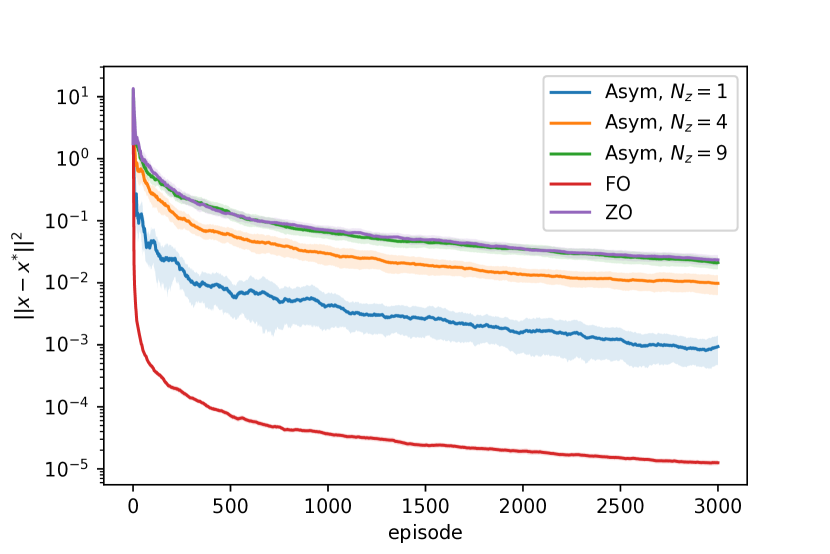
Figure 1: Nash equilibrium convergence achieved by the pure first-order method (FO) and the pure zeroth-order method (ZO), and our asymmetric feedback learning algorithm (Asym) with different values of $N_{z}$. The solid lines and shades are averages and standard deviations over 50 runs.

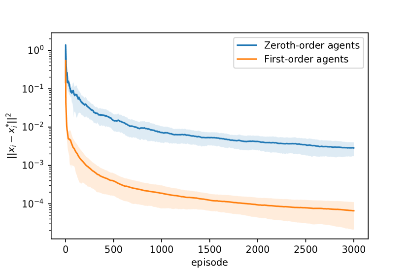
Figure 2: Average error to Nash equilibrium point of first-order agents and zeroth-order agents achieved by Algorithm 1 when $N_{z}=5$. The solid lines and shades are averages and standard deviations over 50 runs.

We run Algorithm 1 with different values of $N_{z}$, as well as the pure first-order method in (8) and the pure zeroth-order method in (10). We choose the step sizes $\eta_{f,t}=\eta_{z,t}=\frac{0.6}{t}$ and the parameter $\delta=\frac{0.5}{t}$. Fig. 1 illustrates the convergence rate of these algorithms. We observe that our asymmetric feedback learning algorithm with different values of $N_{z}$ always performs worse than the pure first-order method but better than the pure zeroth-order method, which agrees with Theorem 2. Besides, a larger value of $N_{z}$, which means that fewer agents have access to first-order gradient feedback, leads to a slower convergence rate; when $N_{z}$ approaches $N$, the convergence rate is similar to that of the pure zeroth-order method.

Fig. 2 illustrates the error between the action $x_{i}$ and the corresponding Nash equilibrium $x^{*}_{i}$ for every agent $i$. We term the agents with access to first-order gradient feedback and zeroth-order oracles as first-order agents and zeroth-order agents, respectively. We select $N_{z}=5$ and compute the average error to the Nash equilibrium for first-order agents and zeroth-order agents. As shown in Fig. 2, the agents with access to first-order gradient feedback converge faster than the agents that ony have access to zeroth-order oracles.

VI-B Risk-averse Cournot Game

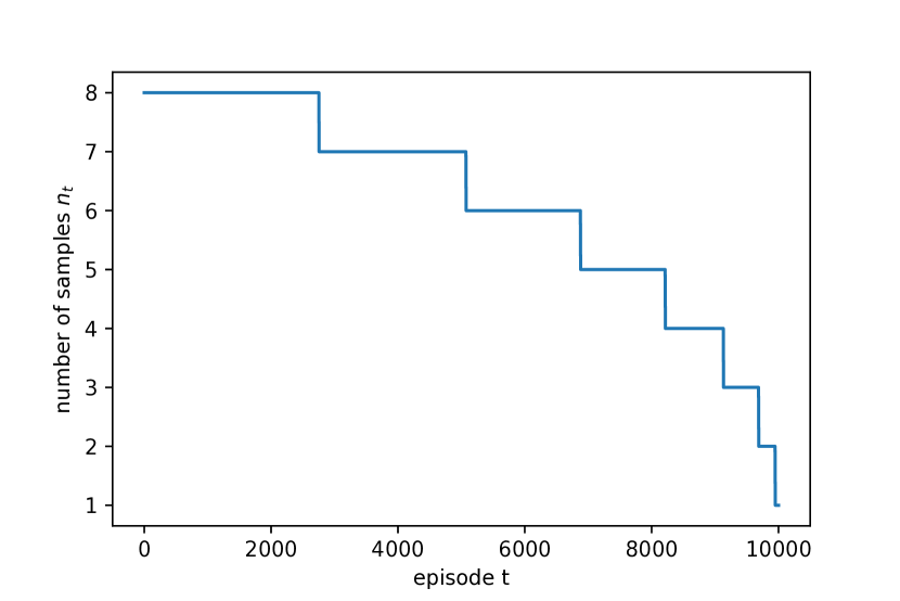
Figure 3: The number of samples of Algorithm 1 and the pure zeroth-order method (Algorithm 1 in [6]).

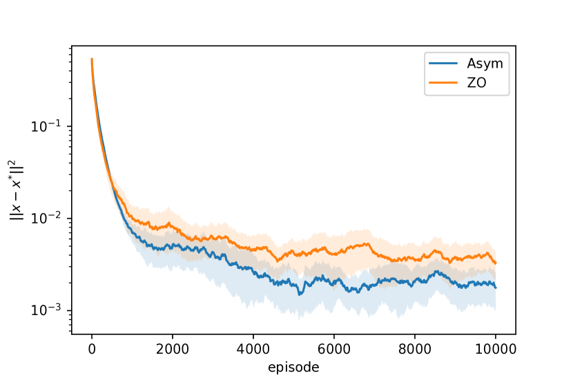
Figure 4: Error to Nash equilibrium point achieved by Algorithm 1 and the pure zeroth-order method (ZO) in risk-averse games. The solid lines and shades are averages and standard deviations over 50 runs.

Consider a market with two agents, i.e., $N=2$. Each agent decides the quantity $x_{i}$, $i=1,2$. The stochastic cost of each agent is defined by $J_{i}(x)=-(2-\sum_{j=1}^{2}x_{j})x_{i}+0.2x_{i}+\xi_{i}x_{i}+1$, where $\xi_{i}$ is a random variable used to represent the uncertainty in the market. Agents aim to minimize the risk of incurring high costs, i.e., agents are risk-averse. We use CVaR as the risk measure and denote the risk level of each agent $i$ by $\alpha_{i}$. It is well known that the CVaR value represents the average of the worst $\alpha_{i}$ percent of the stochastic cost, and when $\alpha_{i}=1$, it is equivalent to the risk-neutral case. Let agent $1$ select the risk level $\alpha_{1}=0.5$ while agent $2$ is risk-neutral, so $\alpha_{2}=1$. The objective functions of these two agents are $\mathcal{C}_{1}(x):={\rm{CVaR}}_{\alpha_{1}}[J_{1}(x,\xi_{1})]$, $\mathcal{C}_{2}(x):=\mathbb{E}[J_{2}(x,\xi_{2})]$, respectively.

The gradient of the CVaR function is hard to compute in most cases even when the function $J_{1}(x,\xi_{1})$ is completely known [40]. We assume that given the played action profile $x$, the risk-averse agent does not have access to gradient feedback but only to the cost feedback $J_{1}(x,\xi_{1})$. The risk-neutral agent has access to gradient feedback $\nabla_{2}\mathcal{C}_{2}(x)$.

Since the CVaR value cannot be estimated from only one sample, we use the sampling strategy proposed in [6] that uses a decreasing number of samples with the number of iterations. The number of samples $n_{t}$ chosen here is shown in Fig. 3. With this sampling strategy, the agents have $n_{t}$ samples at episode $t$ to estimate the CVaR values.

Let $\xi_{i}\sim U(0,0.4)$ be a uniform random variable. Then, we can obtain an explicit expression of the cost function $\mathcal{C}_{1}(x)$. Further, using the first-order optimality condition we can compute the Nash equilibrium to be $(0.4667,0.5667)$. We run Algorithm 1 and the pure zeroth-order algorithm (Algorithm 1 in [6]), and select the step size $\eta_{t}=\frac{0.005}{t}$ and the parameter $\delta=\frac{0.5}{t}$ for both algorithms. Fig. 4 shows that our asymmetric feedback learning algorithm converges faster than the pure zeroth-order method.

VII Conclusion

In this work, we proposed a asymmetric feedback learning algorithm for online convex games in which the agents update their actions using either first-order gradient feedback or zeroth-order oracles. We showed that our algorithm achieves no-regret learning for convex games and last-iterate Nash equilibrium convergence for strongly monotone games. Moreover, we theoretically showed that the performance of our algorithm always lies between that of the pure first-order method and the zeroth-order method. We illustrated our algorithm on deterministic and stochastic risk-averse Cournot games. Future research includes the study of a general framework for asymmetric algorithms where the agents can follow multiple strategies.

-A Proof of Lemma 1

1) Since the function $\mathcal{C}_{i}(x)$ is convex in $x_{i}$ for any fixed $x_{-i}$, we have that $\mathcal{C}_{i_{z}}(x_{z},x_{f,t})$ is convex in $x_{i_{z}}$ and thus $\mathcal{C}_{i_{z},t}(x_{z})$ is convex in $x_{i_{z}}$. Therefore, for any $p_{1},p_{2}\in\mathcal{X}_{i_{z}}^{\delta_{t}}$ and $\theta\in[0,1]$, we have that $\mathcal{C}_{i_{z},t}(\theta p_{1}+(1-\theta)p_{2},x_{-i_{z}})\leq\theta\mathcal{C}_{i_{z},t}(p_{1},x_{-i_{z}})+(1-\theta)\mathcal{C}_{i_{z},t}(p_{2},x_{-i_{z}})$. Based on this, it gives that

$$\mathcal{C}_{i_{z},t}^{\delta_{t}}(\theta p_{1}+(1-\theta)p_{2},x_{-i_{z}})$$

$$=\mathbb{E}\big{[}\mathcal{C}_{i_{z},t}(\theta p_{1}+(1-\theta)p_{2}+\delta_{t}w_{i_{z}},x_{-i_{z}}+\delta_{t}u_{-i_{z}})\big{]}$$

$$=\mathbb{E}\big{[}\mathcal{C}_{i_{z},t}(\theta(p_{1}+\delta_{t}w_{i_{z}})+(1-\theta)(p_{2}+\delta_{t}w_{i_{z}}),$$

$$\quad x_{-i_{z}}+\delta_{t}u_{-i_{z}})\big{]}$$

$$\leq\mathbb{E}\big{[}\theta\mathcal{C}_{i_{z},t}(p_{1}+\delta_{t}w_{i_{z}},x_{-i_{z}}+\delta_{t}u_{-i_{z}})$$

$$\quad+(1-\theta)\mathcal{C}_{i_{z},t}(p_{2}+\delta_{t}w_{i_{z}},x_{-i_{z}}+\delta_{t}u_{-i_{z}})\big{]}$$

$$=\theta\mathcal{C}_{i_{z},t}^{\delta_{t}}(p_{1},x_{-i_{z}})+(1-\theta)\mathcal{C}_{i_{z},t}^{\delta_{t}}(p_{2},x_{-i_{z}}),$$

where the expectations above are taken with respect to $w_{i_{z}}\sim\mathbb{B}$ and $u_{-i_{z}}\sim\mathbb{S}_{-i_{z}}$. The proof is complete.

2) Since the function $\mathcal{C}_{i}(x)$ is $L_{0}$-Lipschitz continuous in $x$, we have that $\mathcal{C}_{i_{z},t}(x_{z})$ is $L_{0}$-Lipschitz continuous in $x_{z}$. Thus, for arbitrary two points $x_{z},x_{z}^{\prime}\in$ we have that $|\mathcal{C}_{i_{z},t}^{\delta_{t}}(x_{z})-\mathcal{C}_{i_{z},t}^{\delta_{t}}(x_{z}^{\prime})|=|\mathop{\mathbb{E}}_{w_{i_{z}}\sim\mathbb{B},u_{-i_{z}}\sim\mathbb{S}_{-i_{z}}}[\mathcal{C}_{i_{z},t}(x_{i_{z}}+\delta_{t}w_{i_{z}},x_{-i_{z}}+\delta_{t}u_{-i_{z}})-\mathcal{C}_{i_{z},t}(x_{i_{z}}^{\prime}+\delta_{t}w_{i_{z}},x_{-i_{z}}^{\prime}+\delta_{t}u_{-i_{z}})]|\leq\mathop{\mathbb{E}}_{w_{i_{z}}\sim\mathbb{B},u_{-i_{z}}\sim\mathbb{S}_{-i_{z}}}[L_{0}\left\|x_{z}-x_{z}^{\prime}\right\|]\leq L_{0}\left\|x_{z}-x_{z}^{\prime}\right\|$. The proof is complete.

3) From the definition of $\mathcal{C}_{i_{z},t}$, it directly follows that $|\mathcal{C}_{i_{z},t}^{\delta_{t}}(x_{z})-\mathcal{C}_{i_{z},t}(x_{z})|=|\mathop{\mathbb{E}}_{w_{i_{z}}\sim\mathbb{B},u_{-i_{z}}\sim\mathbb{S}_{-i_{z}}}[\mathcal{C}_{i_{z},t}(x_{i_{z}}+\delta_{t}w_{i_{z}},x_{-i_{z}}+\delta_{t}u_{-i_{z}})-\mathcal{C}_{i_{z},t}(x_{z})]|\leq|\mathop{\mathbb{E}}_{w_{i_{z}}\sim\mathbb{B},u_{-i_{z}}\sim\mathbb{S}_{-i_{z}}}\left\|L_{0}\delta_{t}(w_{i_{z}},u_{-i_{z}})\right\||\leq L_{0}\delta_{t}\sqrt{N_{z}}$.

4) The proof of this claim can be directly adapted from Lemma C.1 in [8] and thus omitted.

-B Proof of Theorem 1

We first focus on the regret analysis of agents with first-order gradient feedback. Define $y_{i_{f}}^{*}:=\mathop{\rm{argmin}}_{x_{i_{f}}\in\mathcal{X}_{i_{f}}}\sum_{t=1}^{T}\mathcal{C}_{i_{f}}(x_{i_{f}},x_{-i_{f},t},\hat{x}_{z,t})$. From the update rule (6), we have that

$$\left\|x_{i_{f},t+1}-y_{i_{f}}^{*}\right\|^{2}$$

$$=\left\|\mathcal{P}_{\mathcal{X}_{i_{f}}}\Big{(}x_{i_{f},t}-\eta_{f,t}\nabla_{i_{f}}\mathcal{C}_{i_{f}}(x_{f,t},\hat{x}_{z,t})\Big{)}-y_{i_{f}}^{*}\right\|^{2}$$

$$\leq\left\|x_{i_{f},t}-\eta_{f,t}\nabla_{i_{f}}\mathcal{C}_{i_{f}}(x_{f,t},\hat{x}_{z,t})-y_{i_{f}}^{*}\right\|^{2}$$

$$\leq\left\|x_{i_{f},t}-y_{i_{f}}^{*}\right\|^{2}+\eta_{f,t}^{2}\left\|\nabla_{i_{f}}\mathcal{C}_{i_{f}}(x_{f,t},\hat{x}_{z,t})\right\|^{2}$$

$$\quad-2\eta_{f,t}\left\langle\nabla_{i_{f}}\mathcal{C}_{i_{f}}(x_{f,t},\hat{x}_{z,t}),x_{i_{f},t}-y_{i_{f}}^{*}\right\rangle,$$ (13)

where the first inequality is due to the facts that $\mathcal{P}_{\mathcal{X}_{i_{f}}}(y_{i_{f}}^{*})=y_{i_{f}}^{*}$ and the projection operator is non-expansive. From the convexity of the function $\mathcal{C}_{i_{f}}(x)$ in $x_{i_{f}}$, we have that

$${\rm{R}}_{i_{f}}=\sum_{t=1}^{T}\mathcal{C}_{i_{f}}(x_{f,t},\hat{x}_{z,t})-\sum_{t=1}^{T}\mathcal{C}_{i_{f}}(y_{i_{f}}^{*},x_{-i_{f},t},\hat{x}_{z,t})$$

$$\leq\sum_{t=1}^{T}\left\langle\nabla_{i_{f}}\mathcal{C}_{i_{f}}(x_{f,t},\hat{x}_{z,t}),x_{i_{f},t}-y_{i_{f}}^{*}\right\rangle$$

$$\leq\sum_{t=1}^{T}\frac{1}{2\eta_{f,t}}\Big{(}\left\|x_{i_{f},t}-y_{i_{f}}^{*}\right\|^{2}-\left\|x_{i_{f},t+1}-y_{i_{f}}^{*}\right\|^{2}$$

$$\quad+\eta_{f,t}^{2}\left\|\nabla_{i_{f}}\mathcal{C}_{i_{f}}(x_{f,t},\hat{x}_{z,t})\right\|^{2}\Big{)}$$

$$\leq\sum_{t=1}^{T}\left\|x_{i_{f},t}-y_{i_{f}}^{*}\right\|^{2}\Big{(}\frac{1}{2\eta_{f,t}}-\frac{1}{2\eta_{f,t-1}}\Big{)}+\sum_{t=1}^{T}\frac{\eta_{f,t}L_{0}^{2}}{2}$$

$$\leq\frac{D^{2}}{2}\sum_{t=1}^{T}\Big{(}\frac{1}{\eta_{f,t}}-\frac{1}{\eta_{f,t-1}}\Big{)}+\sum_{t=1}^{T}\frac{\eta_{f,t}L_{0}^{2}}{2}$$

$$\leq\frac{D^{2}}{2\eta_{f,T}}+\sum_{t=1}^{T}\frac{\eta_{f,t}L_{0}^{2}}{2}$$

$$\leq\frac{\sqrt{T}}{2}(D^{2}+2L_{0}^{2}),$$

where the second inequality follows from (-B) and the last inequality follows since $\eta_{f,t}=\frac{1}{\sqrt{t}}$ and $\sum_{t=1}^{T}\frac{1}{\sqrt{t}}\leq 2\sqrt{T}$. The proof for the agents with first-order gradient feedback is complete.

Next we turn to the regret analysis of the agents with zeroth-order oracles. Define $y_{i_{z}}^{*}:=\mathop{\rm{argmin}}_{x_{i_{z}}\in\mathcal{X}_{i_{z}}}\sum_{t=1}^{T}\mathcal{C}_{i_{z}}(x_{i_{z}},\hat{x}_{-i_{z},t},x_{f,t})$ and $y_{i_{z}}^{\delta_{t}}:=(1-\delta_{t})y_{i_{z}}^{*}$. Since $y_{i_{z}}^{*}\in\mathcal{X}_{i_{z}}$, we have $y_{i_{z}}^{\delta_{t}}\in\mathcal{X}_{i_{z}}^{\delta_{t}}$.

By virtue of the update rule (4), we have that

$$\left\|x_{i_{z},t+1}-y_{i_{z}}^{\delta_{t}}\right\|^{2}$$

$$=\left\|\mathcal{P}_{\mathcal{X}_{i_{z}}^{\delta_{t}}}\Big{(}x_{i_{z},t}-\eta_{z,t}{g}_{i_{z},t}\Big{)}-y_{i_{z}}^{\delta_{t}}\right\|^{2}$$

$$\leq\left\|x_{i_{z},t}-y_{i_{z}}^{\delta_{t}}\right\|^{2}+\eta_{z,t}^{2}\left\|{g}_{i_{z},t}\right\|^{2}$$

$$\quad-2\eta_{z,t}\left\langle x_{i_{z},t}-y_{i_{z}}^{\delta_{t}},g_{i_{z},t}\right\rangle,$$ (14)

where the last inequality is due to the fact that $\mathcal{P}_{\mathcal{X}_{i_{z}}^{\delta_{t}}}(y_{i_{z}}^{\delta_{t}})=y_{i_{z}}^{\delta_{t}}$. Taking expectations of both sides on the inequality (-B), we obtain that

$$\mathbb{E}\left\|x_{i_{z},t+1}-y_{i_{z}}^{\delta_{t}}\right\|^{2}\leq\mathbb{E}\left\|x_{i_{z},t}-y_{i_{z}}^{\delta_{t}}\right\|^{2}+\frac{\eta_{z,t}^{2}d^{2}U^{2}}{\delta_{t}^{2}}$$

$$-2\eta_{z,t}\mathbb{E}\left[\left\langle x_{i_{z},t}-y_{i_{z}}^{\delta_{t}},\nabla_{i_{z}}\mathcal{C}_{i_{z},t}^{\delta_{t}}(x_{z,t})\right\rangle\right],$$ (15)

where the inequality follows from the fact that $\left\|g_{i_{z},t}\right\|=\left\|\frac{d}{\delta_{t}}\mathcal{C}_{i_{z}}(\hat{x}_{z,t},x_{f,t})u_{i_{z},t}\right\|\leq\frac{dU}{\delta_{t}}$. Then, we have that

$${\rm{R}}_{i_{z}}=\sum_{t=1}^{T}\mathcal{C}_{i_{z}}(\hat{x}_{z,t},x_{f,t})-\sum_{t=1}^{T}\mathcal{C}_{i_{z}}(y_{i_{z}}^{*},\hat{x}_{-i_{z},t},x_{f,t})$$

$$=\sum_{t=1}^{T}\Big{(}\mathcal{C}_{i_{z},t}(\hat{x}_{z,t})-\mathcal{C}_{i_{z},t}(y_{i_{z}}^{*},\hat{x}_{-i_{z},t})-\mathcal{C}_{i_{z},t}({x}_{z,t})$$

$$\quad+\mathcal{C}_{i_{z},t}({x}_{z,t})-\mathcal{C}_{i_{z},t}(y_{i_{z}}^{*},{x}_{-i_{z},t})+\mathcal{C}_{i_{z},t}(y_{i_{z}}^{*},{x}_{-i_{z},t})\Big{)}$$

$$\leq\sum_{t=1}^{T}\Big{(}\mathcal{C}_{i_{z},t}({x}_{z,t})-\mathcal{C}_{i_{z},t}(y_{i_{z}}^{*},{x}_{-i_{z},t})+2L_{0}\delta_{t}\sqrt{N_{z}}\Big{)}$$

$$\leq\sum_{t=1}^{T}\Big{(}\mathcal{C}_{i_{z},t}^{\delta_{t}}({x}_{z,t})-\mathcal{C}_{i_{z},t}^{\delta_{t}}(y_{i_{z}}^{*},{x}_{-i_{z},t})+4L_{0}\delta_{t}\sqrt{N_{z}}\Big{)}$$

$$=\sum_{t=1}^{T}\Big{(}\mathcal{C}_{i_{z},t}^{\delta_{t}}({x}_{z,t})-\mathcal{C}_{i_{z},t}^{\delta_{t}}(y_{i_{z}}^{\delta_{t}},{x}_{-i_{z},t})+\mathcal{C}_{i_{z},t}^{\delta_{t}}(y_{i_{z}}^{\delta_{t}},{x}_{-i_{z},t})$$

$$\quad-\mathcal{C}_{i_{z},t}^{\delta_{t}}(y_{i_{z}}^{*},{x}_{-i_{z},t})+4L_{0}\delta_{t}\sqrt{N_{z}}\Big{)}$$

$$\leq\sum_{t=1}^{T}\Big{(}\mathcal{C}_{i_{z},t}^{\delta_{t}}({x}_{z,t})-\mathcal{C}_{i_{z},t}^{\delta_{t}}(y_{i_{z}}^{\delta_{t}},{x}_{-i_{z},t})+L_{0}\delta_{t}D$$

$$\quad+4L_{0}\delta_{t}\sqrt{N_{z}}\Big{)}$$

$$\leq\sum_{t=1}^{T}\left\langle x_{i_{z},t}-y_{i_{z}}^{\delta_{t}},\nabla_{i_{z}}\mathcal{C}_{i_{z},t}^{\delta}(x_{z,t})\right\rangle$$

$$\quad+L_{0}(D+4\sqrt{N_{z}})\sum_{t=1}^{T}\delta_{t},$$ (16)

where the first inequality follows from the second item in Lemma 1, the second inequality follows from the third item in Lemma 1, and the third inequality follows since $|\mathcal{C}_{i_{z},t}^{\delta_{t}}(y_{i_{z}}^{\delta_{t}},{x}_{-i_{z},t})-\mathcal{C}_{i_{z},t}^{\delta_{t}}(y_{i_{z}}^{*},{x}_{-i_{z},t})|\leq L_{0}\delta_{t}\left\|y_{i_{z}}^{*}\right\|\leq L_{0}\delta_{t}D$. The last inequality follows from the first item in Lemma 1. Define $\frac{1}{\eta_{z,0}}=0$. Substituting the inequality (-B) into the inequality (-B), we have that

$${\rm{R}}_{i_{z}}$$

$$\leq\sum_{t=1}^{T}\frac{1}{2\eta_{z,t}}\Big{(}\mathbb{E}\left\|x_{i_{z},t}-y_{i_{z}}^{\delta_{t}}\right\|^{2}-\mathbb{E}\left\|x_{i_{z},t+1}-y_{i_{z}}^{\delta_{t}}\right\|^{2}\Big{)}$$

$$\quad+\sum_{t=1}^{T}\frac{\eta_{z,t}d^{2}U^{2}}{2\delta_{t}^{2}}+L_{0}(D+4\sqrt{N_{z}})\sum_{t=1}^{T}\delta_{t}$$

$$=\sum_{t=1}^{T}\frac{1}{2\eta_{z,t}}\Big{(}\mathbb{E}\left\|x_{i_{z},t}-y_{i_{z}}^{\delta_{t}}\right\|^{2}-\mathbb{E}\left\|x_{i_{z},t+1}-y_{i_{z}}^{\delta_{t+1}}\right\|^{2}$$

$$\quad+\mathbb{E}\left\|x_{i_{z},t+1}-y_{i_{z}}^{\delta_{t+1}}\right\|^{2}-\mathbb{E}\left\|x_{i_{z},t+1}-y_{i_{z}}^{\delta_{t}}\right\|^{2}\Big{)}$$

$$\quad+L_{0}(D+4\sqrt{N_{z}})\sum_{t=1}^{T}\delta_{t}$$

$$\leq\frac{1}{2}\sum_{t=1}^{T}\mathbb{E}\left\|x_{i_{z},t}-y_{i_{z}}^{\delta_{t}}\right\|^{2}(\frac{1}{\eta_{z,t}}-\frac{1}{\eta_{z,t-1}})$$

$$\quad+\sum_{t=1}^{T}\frac{1}{2\eta_{z,t}}\mathbb{E}\left[\langle y_{i_{z}}^{\delta_{t+1}}-y_{i_{z}}^{\delta_{t}},y_{i_{z}}^{\delta_{t}}+y_{i_{z}}^{\delta_{t+1}}-2x_{i_{z},t+1}\rangle\right]$$

$$\quad+L_{0}(D+4\sqrt{N_{z}})\sum_{t=1}^{T}\delta_{t}$$

$$\leq\frac{D^{2}}{2\eta_{z,T}}+L_{0}(D+4\sqrt{N_{z}})\sum_{t=1}^{T}\delta_{t}$$

$$\quad+\sum_{t=1}^{T}\frac{1}{2\eta_{z,t}}\left\|y_{i_{z}}^{\delta_{t+1}}-y_{i_{z}}^{\delta_{t}}\right\|2D$$

$$\leq\frac{D^{2}}{2\eta_{z,T}}+L_{0}(D+4\sqrt{N_{z}})\sum_{t=1}^{T}\delta_{t}+\sum_{t=1}^{T}\frac{(\delta_{t}-\delta_{t+1})D^{2}}{\eta_{z,t}}$$

$$\leq\frac{D^{2}}{2\eta_{z,T}}+L_{0}(D+4\sqrt{N_{z}})\sum_{t=1}^{T}\delta_{t}$$

$$\quad+D^{2}\sum_{t=1}^{T}\delta_{t}\Big{(}\frac{1}{\eta_{z,t}}-\frac{1}{\eta_{z,t-1}}\Big{)},$$ (17)

where in the second and last inequalities we use the definition $\frac{1}{\eta_{z,0}}=0$. The fourth inequality holds since $\left\|y_{i_{z}}^{\delta_{t+1}}-y_{i_{z}}^{\delta_{t}}\right\|=\left\|(\delta_{t+1}-\delta_{t})y_{i_{z}}^{*}\right\|\leq(\delta_{t}-\delta_{t+1})D$. Substituting $\eta_{z,t}=\frac{1}{N_{z}^{\frac{1}{4}}t^{\frac{3}{4}}}$ and $\delta_{t}=\frac{1}{N_{z}^{\frac{1}{4}}t^{\frac{1}{4}}}$ into the inequality (-B), we have

$${\rm{R}}_{i_{z}}$$

$$\leq\frac{D^{2}N_{z}^{\frac{1}{4}}T^{\frac{3}{4}}}{2}+\frac{L_{0}(D+4\sqrt{N_{z}})}{N_{z}^{\frac{1}{4}}}\sum_{t=1}^{T}\frac{1}{t^{\frac{1}{4}}}$$

$$\quad+D^{2}\sum_{t=1}^{T}\frac{1}{t^{\frac{1}{4}}}\big{(}t^{\frac{3}{4}}-(t-1)^{\frac{3}{4}}\big{)}$$

$$\leq\frac{D^{2}N_{z}^{\frac{1}{4}}T^{\frac{3}{4}}}{2}+\frac{L_{0}(D+4\sqrt{N_{z}})}{N_{z}^{\frac{1}{4}}}\sum_{t=1}^{T}\frac{1}{t^{\frac{1}{4}}}+D^{2}\sum_{t=1}^{T}\frac{1}{t^{\frac{1}{4}}}$$

$$\leq\frac{D^{2}N_{z}^{\frac{1}{4}}T^{\frac{3}{4}}}{2}+\frac{4L_{0}(D+4\sqrt{N_{z}})}{3N_{z}^{\frac{1}{4}}}T^{\frac{3}{4}}+\frac{4D^{2}}{3}T^{\frac{3}{4}}$$

$$=\mathcal{O}\left(N_{Z}^{\frac{1}{4}}T^{\frac{3}{4}}\right),$$

where the last inequality follows from the fact that $\sum_{t=1}^{T}t^{-\frac{1}{4}}\leq 1+\int_{1}^{T}t^{-\frac{1}{4}}dt\leq\frac{4}{3}T^{\frac{3}{4}}$. The second inequality holds since $f(t):=t^{\frac{3}{4}}-(t-1)^{\frac{3}{4}}\leq 1$ for all $t\geq 1$, which is easily verified through computing the derivative of $f(t)$. The proof is complete.

-C Proof of Proposition 1

From the update rule (8), we have that

$$\left\|x_{i,t+1}-x_{i}^{*}\right\|^{2}$$

$$\leq\left\|x_{i,t}-x_{i}^{*}\right\|^{2}+\eta_{t}^{2}\left\|\nabla_{i}\mathcal{C}_{i}(x_{t})\right\|^{2}$$

$$\quad-2\eta_{t}\langle x_{i,t}-x_{i}^{*},\nabla_{i}\mathcal{C}_{i}(x_{t})\rangle$$

$$\leq\left\|x_{i,t}-x_{i}^{*}\right\|^{2}+\eta_{t}^{2}\left\|\nabla_{i}\mathcal{C}_{i}(x_{t})\right\|^{2}$$

$$\quad-2\eta_{t}\langle x_{i,t}-x_{i}^{*},\nabla_{i}\mathcal{C}_{i}(x_{t})-\nabla_{i}\mathcal{C}_{i}(x^{*})\rangle,$$ (18)

where the last inequality follows from the first-order optimality condition. Summing the inequality (-C) over $i=1,\ldots,N$ and using the strong monotonicity condition (2), it gives

$$\left\|x_{t+1}-x^{*}\right\|^{2}\leq(1-2m\eta_{t})\left\|x_{t}-x^{*}\right\|^{2}+\eta_{t}^{2}L_{0}^{2}N.$$ (19)

Substituting $\eta_{t}=\frac{1}{mt}$ into the inequality (19), we have that

$$\left\|x_{t+1}-x^{*}\right\|^{2}\leq(1-\frac{2}{t})\left\|x_{t}-x^{*}\right\|^{2}+\frac{L_{0}^{2}N}{m^{2}t^{2}}.$$ (20)

In what follows, we prove that the inequality (20) implies that

$$\left\|x_{t}-x^{*}\right\|^{2}\leq\frac{L_{0}^{2}N}{m^{2}t}+\frac{D^{2}}{t},\;\forall t\geq 1.$$ (21)

We use the mathematical inductive method. Firstly, since $A_{1}\leq D^{2}$, the statement for the base case holds. Secondly, assuming that the statement holds at time step $t$, it gives that

$$\left\|x_{t+1}-x^{*}\right\|^{2}\leq (1-\frac{2}{t})\Big{(}\frac{L_{0}^{2}N}{m^{2}t}+\frac{D^{2}}{t}\Big{)}+\frac{L_{0}^{2}N}{m^{2}t^{2}}$$

$$= (1-\frac{1}{t})\frac{L_{0}^{2}N}{m^{2}t}+(1-\frac{2}{t})\frac{D^{2}}{t}$$

$$\leq (1-\frac{1}{t})\frac{c_{1}L_{0}^{2}N}{m^{2}t}+(1-\frac{1}{t})\frac{D^{2}}{t}$$

$$\leq \frac{c_{1}L_{0}^{2}N}{m^{2}(t+1)}+\frac{D^{2}}{t+1},$$

where the last inequality holds since $(1-\frac{1}{t})=\frac{t-1}{t}\leq\frac{t}{t+1}$. It shows that the statement also holds at time step $t+1$ and therefore we can conclude that the statement (21) holds for all $t\geq 1$. Replacing $t$ with $T$ in (21), we can obtain the desired result. The proof is complete.

-D Proof of Proposition 2

Let $x_{t}^{*}:=(1-\delta_{t})x^{*}$ and $x_{i,t}^{*}=(1-\delta_{t})x_{i}^{*}$. Since $x_{i}^{*}\in\mathcal{X}_{i}$, we have $x_{i,t}^{*}\in\mathcal{X}_{i}^{\delta_{t}}$. From the update rule (10), we have

$$\left\|x_{i,t+1}-x_{i,t}^{*}\right\|^{2}$$

$$=\left\|\mathcal{P}_{\mathcal{X}_{i}^{\delta_{t}}}\Big{(}x_{i,t}-\eta_{t}{G}_{i,t}\Big{)}-x_{i,t}^{*}\right\|^{2}$$

$$\leq\left\|x_{i,t}-\eta_{t}{G}_{i,t}-x_{i,t}^{*}\right\|^{2}$$

$$=\left\|x_{i,t}-x_{i,t}^{*}\right\|^{2}+\eta_{t}^{2}\left\|G_{i,t}\right\|^{2}-2\eta_{t}\langle x_{i,t}-x_{i,t}^{*},G_{i,t}\rangle,$$ (22)

where the inequality holds since the projection operator is non-expansive. Taking expectations of both sides on the inequality (-D), it follows that

$$\mathbb{E}[\left\|x_{i,t+1}-x_{i,t}^{*}\right\|^{2}]$$

$$\leq\mathbb{E}[\left\|x_{i,t}-x_{i,t}^{*}\right\|^{2}]-2\eta_{t}\mathbb{E}\Big{[}\left\langle x_{i,t}-x_{i,t}^{*},\nabla_{i}\mathcal{C}_{i}^{{\delta_{t}}}(x_{t})\right\rangle\Big{]}$$

$$\quad+\eta_{t}^{2}\mathbb{E}[\left\|G_{i,t}\right\|^{2}]$$

$$\leq\mathbb{E}[\left\|x_{i,t}-x_{i,t}^{*}\right\|^{2}]+\frac{\eta_{t}^{2}d^{2}U^{2}}{{\delta_{t}^{2}}}-2\eta_{t}\mathbb{E}\Big{[}\langle x_{i,t}-x_{i,t}^{*},$$

$$\quad\nabla_{i}\mathcal{C}_{i}^{{\delta_{t}}}(x_{t})-\nabla_{i}\mathcal{C}_{i}(x_{t})+\nabla_{i}\mathcal{C}_{i}(x_{t})\rangle\Big{]}$$

$$\leq\mathbb{E}[\left\|x_{i,t}-x_{i,t}^{*}\right\|^{2}]+\frac{\eta_{t}^{2}d^{2}U^{2}}{{\delta_{t}^{2}}}+2\eta_{t}L_{1}{\delta_{t}}\sqrt{N}D$$

$$\quad-2\eta_{t}\mathbb{E}[\left\langle x_{i,t}-x_{i,t}^{*},\nabla_{i}\mathcal{C}_{i}(x_{t})\right\rangle]$$

$$=\mathbb{E}[\left\|x_{i,t}-x_{i,t}^{*}\right\|^{2}]+\frac{\eta_{t}^{2}d^{2}U^{2}}{{\delta_{t}^{2}}}+2\eta_{t}L_{1}{\delta_{t}}\sqrt{N}D$$

$$\quad-2\eta_{t}\mathbb{E}[\left\langle x_{i,t}-x_{i,t}^{*},\nabla_{i}\mathcal{C}_{i}(x_{t})-\nabla_{i}\mathcal{C}_{i}(x_{t}^{*})\right\rangle]$$

$$\quad-2\eta_{t}\mathbb{E}[\left\langle x_{i,t}-x_{i,t}^{*},\nabla_{i}\mathcal{C}_{i}(x_{t}^{*})-\nabla_{i}\mathcal{C}_{i}(x^{*})\right\rangle]$$

$$\quad-2\eta_{t}\mathbb{E}[\left\langle x_{i,t}-x_{i,t}^{*},\nabla_{i}\mathcal{C}_{i}(x^{*})\right\rangle]$$

$$\leq\mathbb{E}[\left\|x_{i,t}-x_{i,t}^{*}\right\|^{2}]+\frac{\eta_{t}^{2}d^{2}U^{2}}{{\delta_{t}^{2}}}+2\eta_{t}L_{1}{\delta_{t}}\sqrt{N}D$$

$$\quad-2\eta_{t}\mathbb{E}[\left\langle x_{i,t}-x_{i,t}^{*},\nabla_{i}\mathcal{C}_{i}(x_{t})-\nabla_{i}\mathcal{C}_{i}(x_{t}^{*})\right\rangle]$$

$$\quad-2\eta_{t}\mathbb{E}[\left\langle x_{i,t}-x_{i}^{*}+x_{i}^{*}-x_{i,t}^{*},\nabla_{i}\mathcal{C}_{i}(x^{*})\right\rangle]$$

$$\quad+2\eta_{t}L_{1}\delta_{t}D^{2}$$

$$\leq\mathbb{E}[\left\|x_{i,t}-x_{i,t}^{*}\right\|^{2}]+\frac{\eta_{t}^{2}d^{2}U^{2}}{{\delta_{t}^{2}}}+2\eta_{t}L_{1}{\delta_{t}}\sqrt{N}D$$

$$\quad-2\eta_{t}\mathbb{E}[\left\langle x_{i,t}-x_{i,t}^{*},\nabla_{i}\mathcal{C}_{i}(x_{t})-\nabla_{i}\mathcal{C}_{i}(x_{t}^{*})\right\rangle]$$

$$\quad+2\eta_{t}L_{1}\delta_{t}D^{2}+2\eta_{t}\delta_{t}L_{0}D,$$ (23)

where the third inequality can be obtained by Lemma 2 and the fourth inequality holds since $\left\|\nabla_{i}\mathcal{C}_{i}(x_{t})-\nabla_{i}\mathcal{C}_{i}(x_{t}^{*})\right\|\leq L_{1}\left\|x_{t}-x_{t}^{*}\right\|=L_{1}\delta_{t}\left\|x^{*}\right\|\leq L_{1}\delta_{t}D$. The last inequality follows from the Nash equilibrium first-order optimality condition and the fact that $\left\|x_{i}^{*}-x_{i,t}^{*}\right\|\leq\delta_{t}D$. Summing the inequality (-D) over $i=1,\ldots,N$ and using the strong monotonity condition (2), we have that

$$\mathbb{E}[\left\|x_{t+1}-x_{t}^{*}\right\|^{2}]$$

$$\leq(1-2m\eta_{t})\mathbb{E}[\left\|x_{t}-x_{t}^{*}\right\|^{2}]+\frac{\eta_{t}^{2}d^{2}U^{2}N}{{\delta_{t}^{2}}}$$

$$\quad+2\eta_{t}{\delta_{t}}\big{(}N^{\frac{3}{2}}L_{1}D+NL_{1}D^{2}+NL_{0}D\big{)}.$$ (24)

Define $x_{0}^{*}:=x^{*}$, $\delta_{0}=0$ and recall $\delta_{t}=\frac{1}{N^{\frac{1}{6}}t^{\frac{1}{3}}}$. Then, for all $t\geq 1$, it holds that

$$\left\|x_{t}-x_{t}^{*}\right\|^{2}$$

$$=\left\|x_{t}-x_{t-1}^{*}+x_{t-1}^{*}-x_{t}^{*}\right\|^{2}$$

$$\leq\left\|x_{t}-x_{t-1}^{*}\right\|^{2}+\left\|x_{t-1}^{*}-x_{t}^{*}\right\|^{2}$$

$$\quad+2\left\|x_{t}-x_{t-1}^{*}\right\|\left\|x_{t-1}^{*}-x_{t}^{*}\right\|$$

$$\leq\left\|x_{t}-x_{t-1}^{*}\right\|^{2}+|\delta_{t-1}-\delta_{t}|^{2}D^{2}+2|\delta_{t-1}-\delta_{t}|D^{2},$$ (25)

where the first inequality holds due to the Cauchy–Schwarz inequality. The second inequality holds at $t=1$ since $\left\|x_{0}^{*}-x_{1}^{*}\right\|=\left\|x^{*}-x_{1}^{*}\right\|=\left\|\delta_{1}x^{*}\right\|\leq\delta_{1}D=|\delta_{0}-\delta_{1}|D$. When $t\geq 2$, it is easy to verify that $|\delta_{t-1}-\delta_{t}|=\frac{1}{N^{\frac{1}{6}}}\Big{(}\frac{1}{(t-1)^{\frac{1}{3}}}-\frac{1}{t^{\frac{1}{3}}}\Big{)}\leq\frac{1}{N^{\frac{1}{6}}t^{\frac{4}{3}}}$. When $t=1$, we have $|\delta_{0}-\delta_{1}|=|\delta_{1}|=\frac{1}{N^{\frac{1}{6}}}$. Hence, for all $t\geq 1$, it holds that

$$|\delta_{t-1}-\delta_{t}|\leq\frac{1}{N^{\frac{1}{6}}t^{\frac{4}{3}}}.$$ (26)

Substituting $\eta_{t}=\frac{1}{mt}$, $\delta_{t}=\frac{1}{N^{\frac{1}{6}}t^{\frac{1}{3}}}$, (-D) and (26) into (-D), we have

$$\mathbb{E}[\left\|x_{t+1}-x_{t}^{*}\right\|^{2}]$$

$$\leq(1-2m\eta_{t})\mathbb{E}[\left\|x_{t}-x_{t-1}^{*}\right\|^{2}]+|\delta_{t-1}-\delta_{t}|^{2}D^{2}$$

$$\quad+2|\delta_{t-1}-\delta_{t}|D^{2}+\frac{\eta_{t}^{2}d^{2}U^{2}N}{{\delta_{t}^{2}}}$$

$$\quad+2\eta_{t}{\delta_{t}}\big{(}N^{\frac{3}{2}}L_{1}D+NL_{1}D^{2}+NL_{0}D\big{)}$$

$$\leq(1-\frac{2}{t})\mathbb{E}[\left\|x_{t}-x_{t-1}^{*}\right\|^{2}]+\frac{D^{2}}{N^{\frac{1}{3}}t^{\frac{8}{3}}}+\frac{2D^{2}}{N^{\frac{1}{6}}t^{\frac{4}{3}}}+\frac{N^{\frac{4}{3}}d^{2}U^{2}}{m^{2}t^{\frac{4}{3}}}$$

$$\quad+\frac{2}{mt^{\frac{4}{3}}N^{\frac{1}{6}}}\big{(}N^{\frac{3}{2}}L_{1}D+NL_{1}D^{2}+NL_{0}D\big{)}$$

$$\leq(1-\frac{2}{t})\mathbb{E}[\left\|x_{t}-x_{t-1}^{*}\right\|^{2}]+\frac{3D^{2}}{t^{\frac{4}{3}}}+\frac{N^{\frac{4}{3}}d^{2}U^{2}}{m^{2}t^{\frac{4}{3}}}$$

$$\quad+\frac{2}{mt^{\frac{4}{3}}N^{\frac{1}{6}}}\big{(}N^{\frac{3}{2}}L_{1}D+NL_{1}D^{2}+NL_{0}D\big{)},$$ (27)

for all $t\geq 1$. In what follows, we prove that the inequality (-D) implies the following statement for all $t\geq 1$

$$\mathbb{E}[\left\|x_{t}-x_{t-1}^{*}\right\|^{2}]\leq\frac{1}{t^{\frac{1}{3}}}\Big{(}3D^{2}+\frac{N^{\frac{4}{3}}d^{2}U^{2}}{m^{2}}\Big{)}+\frac{D^{2}}{t}$$

$$\quad+\frac{2}{mt^{\frac{1}{3}}N^{\frac{1}{6}}}\big{(}N^{\frac{3}{2}}L_{1}D+NL_{1}D^{2}+NL_{0}D\big{)}.$$ (28)

We still use the mathematical inductive method. Firstly, the statement for the base case naturally holds since $\left\|x_{1}-x^{*}\right\|^{2}\leq D^{2}$. In what follows, we show that if the inequality holds at time step $t$, it also holds at time step $t+1$. Specifically, (-D) and (-D) yield

$$\mathbb{E}[\left\|x_{t+1}-x_{t}^{*}\right\|^{2}]$$

$$\leq(1-\frac{2}{t})\frac{1}{t^{\frac{1}{3}}}\Big{(}3D^{2}+\frac{N^{\frac{4}{3}}d^{2}U^{2}}{m^{2}}\Big{)}+(1-\frac{2}{t})\frac{D^{2}}{t}$$

$$\quad+(1-\frac{2}{t})\frac{2}{mt^{\frac{1}{3}}N^{\frac{1}{6}}}\big{(}N^{\frac{3}{2}}L_{1}D+NL_{1}D^{2}+NL_{0}D\big{)}$$

$$\quad+\frac{2}{mt^{\frac{4}{3}}N^{\frac{1}{6}}}\big{(}N^{\frac{3}{2}}L_{1}D+NL_{1}D^{2}+NL_{0}D\big{)}$$

$$\quad+\frac{3D^{2}}{t^{\frac{4}{3}}}+\frac{N^{\frac{4}{3}}d^{2}U^{2}}{m^{2}t^{\frac{4}{3}}}$$

$$=(1-\frac{1}{t})\frac{1}{t^{\frac{1}{3}}}\Big{(}3D^{2}+\frac{N^{\frac{4}{3}}d^{2}U^{2}}{m^{2}}\Big{)}+(1-\frac{2}{t})\frac{D^{2}}{t}$$

$$\quad+(1-\frac{1}{t})\frac{2}{mt^{\frac{1}{3}}N^{\frac{1}{6}}}\big{(}N^{\frac{3}{2}}L_{1}D+NL_{1}D^{2}+NL_{0}D\big{)}$$

$$\leq\frac{1}{(t+1)^{\frac{1}{3}}}\Big{(}3D^{2}+\frac{N^{\frac{4}{3}}d^{2}U^{2}}{m^{2}}\Big{)}+(1-\frac{2}{t})\frac{D^{2}}{t}$$

$$\quad+\frac{2}{m(t+1)^{\frac{1}{3}}N^{\frac{1}{6}}}\big{(}N^{\frac{3}{2}}L_{1}D+NL_{1}D^{2}+NL_{0}D\big{)}$$

$$\leq\frac{1}{(t+1)^{\frac{1}{3}}}\Big{(}3D^{2}+\frac{N^{\frac{4}{3}}d^{2}U^{2}}{m^{2}}\Big{)}+\frac{D^{2}}{t+1}$$

$$\quad+\frac{2}{m(t+1)^{\frac{1}{3}}N^{\frac{1}{6}}}\big{(}N^{\frac{3}{2}}L_{1}D+NL_{1}D^{2}+NL_{0}D\big{)},$$ (29)

where the second inequality follows from the fact that

$$(1-\frac{1}{t})\frac{1}{t^{\frac{1}{3}}}=\frac{t-1}{t}\frac{1}{t^{\frac{1}{3}}}<\frac{t}{t+1}\frac{1}{t^{\frac{1}{3}}}<\frac{1}{(t+1)^{\frac{1}{3}}}.$$

The last inequality holds since $(1-\frac{2}{t})\frac{1}{t}\leq\frac{t-1}{t^{2}}\leq\frac{1}{t+1}$. The inequality (-D) shows that the statement also holds at time step $t+1$ and thus the statement (-D) holds for all $t\geq 1$. Recalling the definition of $x_{t}^{*}$, when $t\geq 2$, (-D) yields

$$\mathbb{E}[\left\|x_{t}-x^{*}\right\|^{2}]$$

$$=\mathbb{E}[\left\|x_{t}-x_{t-1}^{*}+x_{t-1}^{*}-x^{*}\right\|^{2}]$$

$$\leq\mathbb{E}[2\left\|x_{t}-x_{t-1}^{*}\right\|^{2}+2\left\|x_{t-1}^{*}-x^{*}\right\|^{2}]$$

$$\leq\frac{2}{t^{\frac{1}{3}}}\Big{(}3D^{2}+\frac{N^{\frac{4}{3}}d^{2}U^{2}}{m^{2}}\Big{)}+\frac{2D^{2}}{t}+\frac{2D^{2}}{(t-1)^{\frac{2}{3}}N^{\frac{1}{3}}}$$

$$\quad+\frac{4}{mt^{\frac{1}{3}}}\big{(}N^{\frac{4}{3}}L_{1}D+N^{\frac{5}{6}}L_{1}D^{2}+N^{\frac{5}{6}}L_{0}D\big{)}.$$ (30)

Replacing $t$ with $T$ in (-D) completes the proof.

-E Proof of Theorem 2

Let

$$x^{*} =(x_{z}^{*},x_{f}^{*}),\;x_{z}^{*}=(x_{1}^{*},x_{2}^{*},\ldots,x_{N_{z}}^{*}),$$

$$x_{f}^{*} =(x_{N_{z}+1}^{*},x_{N_{z}+2}^{*},\ldots,x_{N}^{*}),\;x_{t}=(x_{z,t},x_{f,t}),$$

$$x_{z,t} =(x_{1,t},\ldots,x_{N_{z},t}),\;x_{f,t}=(x_{N_{z}+1,t},\ldots,x_{N,t}),$$

$$x_{t}^{*} =(x_{z,t}^{*},x_{f}^{*}),\;x_{z,t}^{*}=(1-\delta_{t})x_{z}^{*},$$

$$A_{i_{z},t}: =\left\|x_{i_{z},t}-x_{i_{z}}^{*}\right\|^{2},\;A_{i_{f},t}:=\left\|x_{i_{f},t}-x_{i_{f}}^{*}\right\|^{2},$$

$$\bar{A}_{i_{z},t}: =\left\|x_{i_{z},t}-x_{i_{z},t-1}^{*}\right\|^{2},\;\hat{A}_{i_{z},t}:=\left\|x_{i_{z},t}-x_{i_{z},t}^{*}\right\|^{2},$$

$$A_{t}: =\sum_{i_{z}=1}^{N_{z}}A_{i_{z},t}+\sum_{i_{f}=N_{z}+1}^{N}A_{i_{f},t}=\left\|x_{t}-x^{*}\right\|^{2},$$

$$\bar{A}_{t}: =\sum_{i_{z}=1}^{N_{z}}\bar{A}_{i_{z},t}+\sum_{i_{f}=N_{z}+1}^{N}A_{i_{f},t}=\left\|x_{t}-x_{t-1}^{*}\right\|^{2},$$

$$\hat{A}_{t}: =\sum_{i_{z}=1}^{N_{z}}\hat{A}_{i_{z},t}+\sum_{i_{f}=N_{z}+1}^{N}A_{i_{f},t}=\left\|x_{t}-x_{t}^{*}\right\|^{2}.$$

We first focus on the evolution of $A_{i_{f},t}$, i.e., the error dynamics of the agents with first-order gradient feedback. From the update rule (6), we have that

$$A_{i_{f},t+1}=\left\|x_{i_{f},t+1}-x_{i_{f}}^{*}\right\|^{2}$$

$$=\left\|\mathcal{P}_{\mathcal{X}_{i_{f}}}\Big{(}x_{i_{f},t}-\eta_{f,t}\nabla_{i_{f}}\mathcal{C}_{i_{f}}(x_{f,t},\hat{x}_{z,t})\Big{)}-x_{i_{f}}^{*}\right\|^{2}$$

$$\leq\left\|x_{i_{f},t}-\eta_{f,t}\nabla_{i_{f}}\mathcal{C}_{i_{f}}(x_{f,t},\hat{x}_{z,t})-x_{i_{f}}^{*}\right\|^{2}$$

$$\leq\left\|x_{i_{f},t}-x_{i_{f}}^{*}\right\|^{2}+\eta_{f,t}^{2}\left\|\nabla_{i_{f}}\mathcal{C}_{i_{f}}(x_{f,t},\hat{x}_{z,t})\right\|^{2}$$

$$\quad-2\eta_{f,t}\left\langle\nabla_{i_{f}}\mathcal{C}_{i_{f}}(x_{f,t},\hat{x}_{z,t}),x_{i_{f},t}-x_{i_{f}}^{*}\right\rangle$$

$$\leq A_{i_{f},t}-2\eta_{f,t}\left\langle\nabla_{i_{f}}\mathcal{C}_{i_{f}}(x_{f,t},\hat{x}_{z,t}),x_{i_{f},t}-x_{i_{f}}^{*}\right\rangle$$

$$\quad+\eta_{f,t}^{2}L_{0}^{2},$$ (31)

where the first inequality is due to the fact that $\mathcal{P}_{\mathcal{X}_{i_{f}}}(x_{i_{f}}^{*})=x_{i_{f}}^{*}$. Since $x^{*}$ is a Nash equilibrium of the convex game (1), we have that $\langle\nabla_{i_{f}}\mathcal{C}_{i_{f}}(x^{*}),x_{i_{f},t}-x_{i_{f}}^{*}\rangle\geq 0$, $i=1,\ldots,N$. Combining this Nash equilibrium condition with the inequality (-E), we have that

$$A_{i_{f},t+1}$$

$$\leq A_{i_{f},t}+\eta_{f,t}^{2}L_{0}^{2}+2\eta_{f,t}\left\langle\nabla_{i_{f}}\mathcal{C}_{i_{f}}(x^{*}),x_{i_{f},t}-x_{i_{f}}^{*}\right\rangle$$

$$\quad-2\eta_{f,t}\left\langle\nabla_{i_{f}}\mathcal{C}_{i_{f}}(x_{f,t},\hat{x}_{z,t}),x_{i_{f},t}-x_{i_{f}}^{*}\right\rangle$$

$$=A_{i_{f},t}-2\eta_{f,t}\Big{\langle}\nabla_{i_{f}}\mathcal{C}_{i_{f}}(x_{f,t},\hat{x}_{z,t})-\nabla_{i_{f}}\mathcal{C}_{i_{f}}(x_{t}),$$

$$\quad\;x_{i_{f},t}-x_{i_{f}}^{*}\Big{\rangle}+\eta_{f,t}^{2}L_{0}^{2}$$

$$\quad-2\eta_{f,t}\left\langle\nabla_{i_{f}}\mathcal{C}_{i_{f}}(x_{t})-\nabla_{i_{f}}\mathcal{C}_{i_{f}}(x_{t}^{*}),x_{i_{f},t}-x_{i_{f}}^{*}\right\rangle$$

$$\quad-2\eta_{f,t}\left\langle\nabla_{i_{f}}\mathcal{C}_{i_{f}}(x_{t}^{*})-\nabla_{i_{f}}\mathcal{C}_{i_{f}}(x^{*}),x_{i_{f},t}-x_{i_{f}}^{*}\right\rangle$$

$$\leq A_{i_{f},t}+\eta_{f,t}^{2}L_{0}^{2}+2\eta_{f,t}L_{1}\delta_{t}\sqrt{N_{z}}D+2\eta_{f,t}L_{1}\delta_{t}D^{2}$$

$$\quad-2\eta_{f,t}\left\langle\nabla_{i_{f}}\mathcal{C}_{i_{f}}(x_{t})-\nabla_{i_{f}}\mathcal{C}_{i_{f}}(x_{t}^{*}),x_{i_{f},t}-x_{i_{f}}^{*}\right\rangle,$$ (32)

where the last inequality follows from the facts that $\left\|\nabla_{i_{f}}\mathcal{C}_{i_{f}}(x_{f,t},\hat{x}_{z,t})-\nabla_{i_{f}}\mathcal{C}_{i_{f}}(x_{t})\right\|\leq L_{1}\left\|\hat{x}_{z,t}-x_{z,t}\right\|\leq L_{1}\delta_{t}\sqrt{N_{z}}$ and $\left\|\nabla_{i_{f}}\mathcal{C}_{i_{f}}(x_{t}^{*})-\nabla_{i_{f}}\mathcal{C}_{i_{f}}(x^{*})\right\|\leq L_{1}\left\|x_{t}^{*}-x^{*}\right\|=L_{1}\left\|x_{z,t}^{*}-x_{z}^{*}\right\|\leq L_{1}\delta_{t}D$.

Next we turn our attention on the evolution of $\bar{A}_{i_{z},t}$. Similarly, from the update equation (4), we obtain that

$$\bar{A}_{i_{z},t+1}=\left\|x_{i_{z},t+1}-x_{i_{z},t}^{*}\right\|^{2}$$

$$=\left\|\mathcal{P}_{\mathcal{X}_{i_{z}}^{\delta_{t}}}\Big{(}x_{i_{z},t}-\eta_{z,t}g_{i_{z},t}\Big{)}-x_{i_{z},t}^{*}\right\|^{2}$$

$$\leq\left\|x_{i_{z},t}-\eta_{z,t}g_{i_{z},t}-x_{i_{z},t}^{*}\right\|^{2}$$

$$=\hat{A}_{i_{z},t}+\eta_{f,t}^{2}\left\|g_{i_{z},t}\right\|^{2}-2\eta_{z,t}\left\langle g_{i_{z},t},x_{i_{z},t}-x_{i_{z},t}^{*}\right\rangle$$

$$\leq\hat{A}_{i_{z},t}+\frac{\eta_{f,t}^{2}d^{2}U^{2}}{\delta_{t}^{2}}-2\eta_{z,t}\left\langle g_{i_{z},t},x_{i_{z},t}-x_{i_{z},t}^{*}\right\rangle,$$ (33)

where the first inequality follows from the fact that $\mathcal{P}_{\mathcal{X}_{i_{z}}^{\delta_{t}}}\Big{(}x_{i_{z},t}^{*}\Big{)}=x_{i_{z},t}^{*}$ and the projection operator is non-expansive. Taking expectation of both sides of the above inequality (-E), we have that

$$\mathbb{E}[\bar{A}_{i_{z},t+1}]$$

$$\leq\mathbb{E}[\hat{A}_{i_{z},t}]-2\eta_{z,t}\mathbb{E}\left\langle\nabla_{i_{z}}\mathcal{C}^{\delta_{t}}_{i_{z},t}(x_{z,t}),x_{i_{z},t}-x_{i_{z},t}^{*}\right\rangle$$

$$\quad+\frac{\eta_{f,t}^{2}d^{2}U^{2}}{\delta_{t}^{2}}$$

$$\leq\mathbb{E}[\hat{A}_{i_{z},t}]+\frac{\eta_{f,t}^{2}d^{2}U^{2}}{\delta_{t}^{2}}$$

$$\quad-2\eta_{z,t}\mathbb{E}\left\langle\nabla_{i_{z}}\mathcal{C}^{\delta_{t}}_{i_{z},t}(x_{z,t})-\nabla_{i_{z}}\mathcal{C}_{i_{z}}(x_{t}),x_{i_{z},t}-x_{i_{z},t}^{*}\right\rangle$$

$$\quad-2\eta_{z,t}\mathbb{E}\left\langle\nabla_{i_{z}}\mathcal{C}_{i_{z}}(x_{t})-\nabla_{i_{z}}\mathcal{C}_{i_{z}}(x_{t}^{*}),x_{i_{z},t}-x_{i_{z},t}^{*}\right\rangle$$

$$\quad-2\eta_{z,t}\mathbb{E}\left\langle\nabla_{i_{z}}\mathcal{C}_{i_{z}}(x_{t}^{*})-\nabla_{i_{z}}\mathcal{C}_{i_{z}}(x^{*}),x_{i_{z},t}-x_{i_{z},t}^{*}\right\rangle$$

$$\leq\mathbb{E}[\hat{A}_{i_{z},t}]+\frac{\eta_{f,t}^{2}d^{2}U^{2}}{\delta_{t}^{2}}+2\eta_{z,t}L_{1}\delta_{t}D^{2}$$

$$\quad-2\eta_{z,t}\mathbb{E}\left\langle\nabla_{i_{z}}\mathcal{C}^{\delta_{t}}_{i_{z},t}(x_{z,t})-\nabla_{i_{z}}\mathcal{C}_{i_{z}}(x_{t}),x_{i_{z},t}-x_{i_{z},t}^{*}\right\rangle$$

$$\quad-2\eta_{z,t}\mathbb{E}\left\langle\nabla_{i_{z}}\mathcal{C}_{i_{z}}(x_{t})-\nabla_{i_{z}}\mathcal{C}_{i_{z}}(x_{t}^{*}),x_{i_{z},t}-x_{i_{z},t}^{*}\right\rangle,$$ (34)

where the first inequality follows from Lemma 1, the second inequality is due to the Nash equilibrium first-order optimality condition and the last inequality follows since $\left\|\nabla_{i_{z}}\mathcal{C}_{i_{z}}(x_{t}^{*})-\nabla_{i_{z}}\mathcal{C}_{i_{z}}(x^{*})\right\|\leq L_{1}\left\|x_{t}^{*}-x^{*}\right\|\leq L_{1}\delta_{t}D$.

Now we are in a position to bound the term $\left\|\nabla_{i_{z}}C^{\delta_{t}}_{i_{z},t}(x_{z,t})-\nabla_{i_{z}}C_{i_{z}}(x_{t})\right\|$. Since $\mathcal{C}_{i_{z}}$ is bounded and continuous for all $i_{z}\in\mathcal{N}_{z}$, by Lebesgue’s dominated convergence theorem (Chapter 4 in [43]), the order of integration and differentiation can be interchanged. Then, it follows that

$$\nabla_{i_{z}}C^{\delta_{t}}_{i_{z},t}(x_{z,t})$$

$$=\nabla_{i_{z}}\mathbb{E}\left[C_{i_{z},t}(x_{i_{z},t}+\delta_{t}w_{i_{z},t},x_{-i_{z},t}+\delta_{t}u_{-i_{z},t})\right]$$

$$=\mathbb{E}\left[\nabla_{i_{z}}C_{i_{z},t}(x_{i_{z},t}+\delta_{t}w_{i_{z},t},x_{-i_{z},t}+\delta_{t}u_{-i_{z},t})\right]$$

$$=\mathbb{E}\left[\nabla_{i_{z}}C_{i_{z}}(x_{i_{z},t}+\delta_{t}w_{i_{z},t},x_{-i_{z},t}+\delta_{t}u_{-i_{z},t},x_{f,t})\right],$$

where the expectations in the above inequality are taken w.r.t $w_{i_{z},t}\sim\mathbb{B}$ and $u_{-i_{z},t}\sim\mathbb{S}_{-i_{z}}$. Then, we have that

$$\left\|\nabla_{i_{z}}C^{\delta_{t}}_{i_{z},t}(x_{z,t})-\nabla_{i_{z}}C_{i_{z}}(x_{t})\right\|$$

$$\leq L_{1}\delta_{t}\left\|(w_{i_{z},t},u_{-i_{z},t})\right\|\leq L_{1}\delta_{t}\sqrt{N_{z}}.$$ (35)

Substituting (-E) into (-E), we obtain that

$$\mathbb{E}[\bar{A}_{i_{z},t+1}]$$

$$\leq\mathbb{E}[\hat{A}_{i_{z},t}]+\frac{\eta_{f,t}^{2}d^{2}U^{2}}{\delta_{t}^{2}}+2\eta_{z,t}L_{1}\delta_{t}D^{2}$$

$$\quad-2\eta_{z,t}\mathbb{E}\left\langle\nabla_{i_{z}}C_{i_{z}}(x_{t})-\nabla_{i_{z}}\mathcal{C}_{i_{z}}(x_{t}^{*}),x_{i_{z},t}-x_{i_{z},t}^{*}\right\rangle$$

$$\quad+2\eta_{z,t}L_{1}\delta_{t}\sqrt{N_{z}}D.$$ (36)

Define $\delta_{0}=0$ and $x_{i_{z},0}^{*}=x_{i_{z}}^{*}$. From the definition of $\hat{A}_{i_{z},t}$ and $\bar{A}_{i_{z},t}$, we have

$$\hat{A}_{i_{z},t}=\left\|x_{i_{z},t}-x_{i_{z},t-1}^{*}+x_{i_{z},t-1}^{*}-x_{i_{z},t}^{*}\right\|^{2}$$

$$=\bar{A}_{i_{z},t}+\left\|x_{i_{z},t-1}^{*}-x_{i_{z},t}^{*}\right\|^{2}$$

$$\quad+2\langle x_{i_{z},t}-x_{i_{z},t-1}^{*},x_{i_{z},t-1}^{*}-x_{i_{z},t}^{*}\rangle$$

$$\leq\bar{A}_{i_{z},t}+|\delta_{t-1}-\delta_{t}|^{2}D^{2}+2|\delta_{t-1}-\delta_{t}|D^{2},$$ (37)

for all $t\geq 1$. The inequality (-E) holds at $t=1$ since $\left\|x_{i_{z},0}^{*}-x_{i_{z},1}^{*}\right\|=\delta_{1}x_{i_{z}}^{*}\leq|\delta_{0}-\delta_{1}|D$. Substituting (-E) into (-E), we have

$$\mathbb{E}[\bar{A}_{i_{z},t+1}]$$

$$\leq\mathbb{E}[\bar{A}_{i_{z},t}]+|\delta_{t-1}-\delta_{t}|^{2}D^{2}+2|\delta_{t-1}-\delta_{t}|D^{2}$$

$$\quad-2\eta_{z,t}\mathbb{E}\left\langle\nabla_{i_{z}}C_{i_{z}}(x_{t})-\nabla_{i_{z}}\mathcal{C}_{i_{z}}(x_{t}^{*}),x_{i_{z},t}-x_{i_{z},t}^{*}\right\rangle$$

$$\quad+\frac{\eta_{f,t}^{2}d^{2}U^{2}}{\delta_{t}^{2}}+2\eta_{z,t}L_{1}\delta_{t}D^{2}+2\eta_{z,t}L_{1}\delta_{t}\sqrt{N_{z}}D.$$ (38)

Summing (-E) over $i_{f}=N_{z}+1,\ldots,N$ and (-E) over $i_{z}=1,\ldots,N_{z}$ altogether, and setting $\eta_{z,t}=\eta_{f,t}=\eta_{t}$ we have that

$$\mathbb{E}[\bar{A}_{t+1}]=\sum_{i_{z}=1}^{N_{z}}\mathbb{E}\left[\bar{A}_{i_{z},t+1}\right]+\sum_{i_{f}=N_{z}+1}^{N}\mathbb{E}\left[A_{i_{f},t+1}\right]$$

$$\leq\sum_{i_{z}=1}^{N_{z}}\Big{(}\mathbb{E}[\bar{A}_{i_{z},t}]+|\delta_{t-1}-\delta_{t}|^{2}D^{2}+2|\delta_{t-1}-\delta_{t}|D^{2}$$

$$\quad-2\eta_{t}\mathbb{E}\left\langle\nabla_{i_{z}}C_{i_{z}}(x_{t})-\nabla_{i_{z}}\mathcal{C}_{i_{z}}(x_{t}^{*}),x_{i_{z},t}-x_{i_{z},t}^{*}\right\rangle$$

$$\quad+\frac{\eta_{t}^{2}d^{2}U^{2}}{\delta_{t}^{2}}+2\eta_{t}L_{1}\delta_{t}D^{2}+2\eta_{t}L_{1}\delta_{t}\sqrt{N_{z}}D\Big{)}$$

$$\quad+\sum_{i_{f}=N_{z}+1}^{N}\Big{(}\mathbb{E}[A_{i_{f},t}]+\eta_{t}^{2}L_{0}^{2}+2\eta_{t}L_{1}\delta_{t}\sqrt{N_{z}}D$$

$$\quad-2\eta_{t}\mathbb{E}\left\langle\nabla_{i_{f}}\mathcal{C}_{i_{f}}(x_{t})-\nabla_{i_{f}}\mathcal{C}_{i_{f}}(x_{t}^{*}),x_{i_{f},t}-x_{i_{f}}^{*}\right\rangle$$

$$\quad+2\eta_{t}L_{1}\delta_{t}D^{2}\Big{)}$$

$$\leq\mathbb{E}[\bar{A}_{t}]+N_{z}|\delta_{t-1}-\delta_{t}|^{2}D^{2}+2N_{z}|\delta_{t-1}-\delta_{t}|D^{2}$$

$$\quad-2\eta_{t}\sum_{i=1}^{N}\mathbb{E}\left\langle\nabla_{i}C_{i}(x_{t})-\nabla_{i}\mathcal{C}_{i}(x_{t}^{*}),x_{i,t}-x_{i,t}^{*}\right\rangle$$

$$\quad+N_{z}\Big{(}\frac{\eta_{t}^{2}d^{2}U^{2}}{\delta_{t}^{2}}+2\eta_{t}L_{1}\delta_{t}D^{2}+2\eta_{t}L_{1}\delta_{t}\sqrt{N_{z}}D\Big{)}$$

$$\quad+(N-N_{z})\Big{(}\eta_{t}^{2}L_{0}^{2}+2\eta_{t}L_{1}\delta_{t}\sqrt{N_{z}}D+2\eta_{t}L_{1}\delta_{t}D^{2}\Big{)}$$

$$\leq(1-2m\eta_{t})\mathbb{E}[\bar{A}_{t}]+2N_{z}|\delta_{t-1}-\delta_{t}|D^{2}$$

$$\quad+N_{z}|\delta_{t-1}-\delta_{t}|^{2}D^{2}+\frac{\eta_{t}^{2}N_{z}d^{2}U^{2}}{\delta_{t}^{2}}+(N-N_{z})\eta_{t}^{2}L_{0}^{2}$$

$$\quad+2\eta_{t}\delta_{t}NL_{1}(D^{2}+\sqrt{N_{z}}D),$$ (39)

where the last inequality follows from the strong monotonicity condition (2). Recalling $\delta_{t}=\frac{N_{z}^{\frac{1}{6}}}{N^{\frac{1}{3}}t^{\frac{1}{3}}}$, it is easy to verify that

$$|\delta_{t-1}-\delta_{t}|\leq\frac{N_{z}^{\frac{1}{6}}}{N^{\frac{1}{3}}t^{\frac{4}{3}}},$$ (40)

for all $t\geq 1$. The inequality (40) holds at $t=1$ since $|\delta_{0}-\delta_{1}|=\delta_{1}$. Substituting $\eta_{t}=\frac{1}{mt}$, $\delta_{t}=\frac{N_{z}^{\frac{1}{6}}}{N^{\frac{1}{3}}t^{\frac{1}{3}}}$ and (40) into the inequality (-E), we have that

$$\mathbb{E}[\bar{A}_{t+1}]$$

$$\leq(1-\frac{2}{t})\mathbb{E}[\bar{A}_{t}]+\frac{2N_{z}^{\frac{7}{6}}D^{2}}{N^{\frac{1}{3}}t^{\frac{4}{3}}}+\frac{N_{z}^{\frac{4}{3}}D^{2}}{N^{\frac{2}{3}}t^{\frac{8}{3}}}+\frac{d^{2}U^{2}N_{z}^{\frac{2}{3}}N^{\frac{2}{3}}}{m^{2}t^{\frac{4}{3}}}$$

$$\quad+\frac{2N_{z}^{\frac{1}{6}}N^{\frac{2}{3}}L_{1}}{mt^{\frac{4}{3}}}(D^{2}+\sqrt{N_{z}}D)+(N-N_{z})\frac{L_{0}^{2}}{m^{2}t^{2}}$$

$$\leq(1-\frac{2}{t})\mathbb{E}[\bar{A}_{t}]+\frac{2N_{z}^{\frac{2}{3}}N^{\frac{1}{6}}D^{2}}{t^{\frac{4}{3}}}+\frac{N_{z}^{\frac{2}{3}}D^{2}}{t^{\frac{8}{3}}}+\frac{d^{2}U^{2}N_{z}^{\frac{2}{3}}N^{\frac{2}{3}}}{m^{2}t^{\frac{4}{3}}}$$

$$\quad+\frac{2N_{z}^{\frac{1}{6}}N^{\frac{2}{3}}L_{1}}{mt^{\frac{4}{3}}}(D^{2}+\sqrt{N_{z}}D)+(N-N_{z})\frac{L_{0}^{2}}{m^{2}t^{2}}$$

$$\leq(1-\frac{2}{t})\mathbb{E}[\bar{A}_{t}]+\frac{N_{z}^{\frac{2}{3}}N^{\frac{2}{3}}}{t^{\frac{4}{3}}}\Big{(}3D^{2}+\frac{d^{2}D^{2}}{m^{2}}\Big{)}$$

$$\quad+\frac{2N_{z}^{\frac{1}{6}}N^{\frac{2}{3}}L_{1}}{mt^{\frac{4}{3}}}(D^{2}+\sqrt{N_{z}}D)+(N-N_{z})\frac{L_{0}^{2}}{m^{2}t^{2}},$$ (41)

where the second inequality follows since $N_{z}\leq N$. In what follows, we use the standard mathematical inductive method to prove that for all $t\geq 1$, the following inequality holds:

$$\mathbb{E}[\bar{A}_{t}]\leq \frac{N_{z}^{\frac{2}{3}}N^{\frac{2}{3}}}{t^{\frac{1}{3}}}\Big{(}3D^{2}+\frac{d^{2}D^{2}}{m^{2}}\Big{)}+(N-N_{z})\frac{L_{0}^{2}}{m^{2}t}$$

$$+\frac{2N_{z}^{\frac{1}{6}}N^{\frac{2}{3}}L_{1}}{mt^{\frac{1}{3}}}(D^{2}+\sqrt{N_{z}}D)+\frac{D^{2}}{t}.$$ (42)

Obviously, the inequality (-E) holds at the initial time step $t=1$ since $\bar{A}_{1}\leq D^{2}$. In the following analysis, we show that, if the statement (-E) holds at $t$ time step, it must also hold for the next time step $t+1$. To do so, we combine the inequalities (-E) and (-E), yielding that

$$\mathbb{E}[\bar{A}_{t+1}]$$

$$\leq(1-\frac{2}{t})\Big{(}\frac{N_{z}^{\frac{2}{3}}N^{\frac{2}{3}}}{t^{\frac{1}{3}}}\Big{(}3D^{2}+\frac{d^{2}D^{2}}{m^{2}}\Big{)}+(N-N_{z})\frac{L_{0}^{2}}{m^{2}t}$$

$$\quad+\frac{2N_{z}^{\frac{1}{6}}N^{\frac{2}{3}}L_{1}}{mt^{\frac{1}{3}}}(D^{2}+\sqrt{N_{z}}D)+\frac{D^{2}}{t}\Big{)}$$

$$\quad+\frac{N_{z}^{\frac{2}{3}}N^{\frac{2}{3}}}{t^{\frac{4}{3}}}\Big{(}3D^{2}+\frac{d^{2}D^{2}}{m^{2}}\Big{)}+(N-N_{z})\frac{L_{0}^{2}}{m^{2}t^{2}}$$

$$\quad+\frac{2N_{z}^{\frac{1}{6}}N^{\frac{2}{3}}L_{1}}{mt^{\frac{4}{3}}}(D^{2}+\sqrt{N_{z}}D)$$

$$=(1-\frac{1}{t})\Big{(}\frac{N_{z}^{\frac{2}{3}}N^{\frac{2}{3}}}{t^{\frac{1}{3}}}\Big{(}3D^{2}+\frac{d^{2}D^{2}}{m^{2}}\Big{)}+(N-N_{z})\frac{L_{0}^{2}}{m^{2}t}$$

$$\quad+\frac{2N_{z}^{\frac{1}{6}}N^{\frac{2}{3}}L_{1}}{mt^{\frac{1}{3}}}(D^{2}+\sqrt{N_{z}}D)\Big{)}+(1-\frac{2}{t})\frac{D^{2}}{t}$$

$$\leq\frac{N_{z}^{\frac{2}{3}}N^{\frac{2}{3}}}{(t+1)^{\frac{1}{3}}}\Big{(}3D^{2}+\frac{d^{2}D^{2}}{m^{2}}\Big{)}+(N-N_{z})\frac{L_{0}^{2}}{m^{2}(t+1)}$$

$$\quad+\frac{2N_{z}^{\frac{1}{6}}N^{\frac{2}{3}}L_{1}}{m(t+1)^{\frac{1}{3}}}(D^{2}+\sqrt{N_{z}}D)+\frac{D^{2}}{t+1},$$ (43)

where the last inequality follows since $(1-\frac{1}{t})\frac{1}{t^{\frac{1}{3}}}\leq\frac{t}{t+1}\frac{1}{t^{\frac{1}{3}}}\leq\frac{1}{(t+1)^{\frac{1}{3}}}$ and $(1-\frac{2}{t})\frac{1}{t}\leq(1-\frac{1}{t})\frac{1}{t}\leq\frac{1}{t+1}$. The inequality (-E) shows that the statement (-E) also holds at $t+1$ given that it holds at $t$, and thus we can conclude that the statement (-E) holds for all $t\geq 1$. Finally, we have

$$\mathbb{E}[A_{T}]=\mathbb{E}[\left\|x_{T}-x^{*}\right\|^{2}]$$

$$=\mathbb{E}[\left\|x_{T}-x_{T-1}^{*}+x_{T-1}^{*}-x^{*}\right\|^{2}]$$

$$\leq\mathbb{E}[2\bar{A}_{T}+2\left\|x_{T-1}^{*}-x^{*}\right\|^{2}]$$

$$\leq\frac{2N_{z}^{\frac{2}{3}}N^{\frac{2}{3}}}{T^{\frac{1}{3}}}\Big{(}3D^{2}+\frac{d^{2}D^{2}}{m^{2}}\Big{)}+(N-N_{z})\frac{2L_{0}^{2}}{m^{2}T}$$

$$\quad+\frac{4N_{z}^{\frac{1}{6}}N^{\frac{2}{3}}L_{1}}{mt^{\frac{1}{3}}}(D^{2}+\sqrt{N_{z}}D)+\frac{2D^{2}}{T}+\frac{2N_{z}^{\frac{1}{3}}D^{2}}{N^{\frac{2}{3}}(T-1)^{\frac{2}{3}}}$$

$$=\mathcal{O}\Big{(}N_{z}^{\frac{2}{3}}N^{\frac{2}{3}}T^{-\frac{1}{3}}+(N-N_{z})T^{-1}\Big{)}.$$

The proof is complete.

References

- [1] Martin Zinkevich. Online convex programming and generalized infinitesimal gradient ascent. In Proceedings of International Conference on Machine Learning, pages 928–936, 2003.
- [2] Elad Hazan. Introduction to online convex optimization. Foundations and Trends in Optimization, 2(3-4):157–325, 2016.
- [3] Shai Shalev-Shwartz. Online learning and online convex optimization. Foundations and Trends in Machine Learning, 4(2):107–194, 2012.
- [4] Yurii Nesterov. Lectures on convex optimization, volume 137. Springer, 2018.
- [5] Pier Giuseppe Sessa, Ilija Bogunovic, Maryam Kamgarpour, and Andreas Krause. No-regret learning in unknown games with correlated payoffs. In Proceedings of Advances in Neural Information Processing Systems, pages 13624–13633, 2019.
- [6] Zifan Wang, Yi Shen, and Michael Zavlanos. Risk-averse no-regret learning in online convex games. In Proceedings of International Conference on Machine Learning, pages 22999–23017, 2022.
- [7] Kaiqing Zhang, Zhuoran Yang, and Tamer Başar. Multi-agent reinforcement learning: A selective overview of theories and algorithms. Handbook of Reinforcement Learning and Control, pages 321–384, 2021.
- [8] Mario Bravo, David Leslie, and Panayotis Mertikopoulos. Bandit learning in concave n-person games. In Proceedings of Advances in Neural Information Processing Systems, pages 5666–5676, 2018.
- [9] Panayotis Mertikopoulos, Christos Papadimitriou, and Georgios Piliouras. Cycles in adversarial regularized learning. In Proceedings of the Twenty-Ninth Annual ACM-SIAM Symposium on Discrete Algorithms, pages 2703–2717, 2018.
- [10] Zifan Wang, Yi Shen, Zachary I Bell, Scott Nivison, Michael M Zavlanos, and Karl H Johansson. A zeroth-order momentum method for risk-averse online convex games. In Proceedings of IEEE Conference on Decision and Control, pages 5179–5184, 2022.
- [11] Yu-Guan Hsieh, Kimon Antonakopoulos, and Panayotis Mertikopoulos. Adaptive learning in continuous games: Optimal regret bounds and convergence to Nash equilibrium. In Proceedings of Conference on Learning Theory, pages 2388–2422, 2021.
- [12] Giuseppe Belgioioso, Angelia Nedić, and Sergio Grammatico. Distributed generalized nash equilibrium seeking in aggregative games on time-varying networks. IEEE Transactions on Automatic Control, 66(5):2061–2075, 2020.
- [13] Chung-Wei Lee, Christian Kroer, and Haipeng Luo. Last-iterate convergence in extensive-form games. In Proceedings of Advances in Neural Information Processing Systems, pages 14293–14305, 2021.
- [14] Sebastian Bervoets, Mario Bravo, and Mathieu Faure. Learning with minimal information in continuous games. Theoretical Economics, 15(4):1471–1508, 2020.
- [15] Tatiana Tatarenko and Maryam Kamgarpour. Bandit online learning of Nash equilibria in monotone games. arXiv preprint arXiv:2009.04258, 2020.
- [16] Tatiana Tatarenko and Maryam Kamgarpour. Learning generalized Nash equilibria in a class of convex games. IEEE Transactions on Automatic Control, 64(4):1426–1439, 2018.
- [17] Dario Paccagnan, Basilio Gentile, Francesca Parise, Maryam Kamgarpour, and John Lygeros. Nash and wardrop equilibria in aggregative games with coupling constraints. IEEE Transactions on Automatic Control, 64(4):1373–1388, 2018.
- [18] Paul Frihauf, Miroslav Krstic, and Tamer Basar. Nash equilibrium seeking in noncooperative games. IEEE Transactions on Automatic Control, 57(5):1192–1207, 2011.
- [19] Hamidou Tembine, Quanyan Zhu, and Tamer Başar. Risk-sensitive mean-field games. IEEE Transactions on Automatic Control, 59(4):835–850, 2013.
- [20] Oriol Vinyals, Igor Babuschkin, Wojciech M Czarnecki, Michaël Mathieu, Andrew Dudzik, Junyoung Chung, David H Choi, Richard Powell, Timo Ewalds, and Petko Georgiev. Grandmaster level in StarCraft II using multi-agent reinforcement learning. Nature, 575(7782):350–354, 2019.
- [21] Jack Serrino, Max Kleiman-Weiner, David C Parkes, and Josh Tenenbaum. Finding friend and foe in multi-agent games. In Proceedings of Advances in Neural Information Processing Systems, pages 1251––1261, 2019.
- [22] Yu-Guan Hsieh, Kimon Antonakopoulos, Volkan Cevher, and Panayotis Mertikopoulos. No-regret learning in games with noisy feedback: Faster rates and adaptivity via learning rate separation. In Proceedings of Advances in Neural Information Processing Systems, pages 6544–6556, 2022.
- [23] Tianyi Lin, Zhengyuan Zhou, Panayotis Mertikopoulos, and Michael Jordan. Finite-time last-iterate convergence for multi-agent learning in games. In Proceedings of International Conference on Machine Learning, pages 6161–6171, 2020.
- [24] Noah Golowich, Sarath Pattathil, and Constantinos Daskalakis. Tight last-iterate convergence rates for no-regret learning in multi-player games. In Proceedings of Advances in neural information processing systems, pages 20766–20778, 2020.
- [25] Panayotis Mertikopoulos and Zhengyuan Zhou. Gradient-free online learning in games with delayed rewards. In Proceedings of International Conference on Machine Learning, pages 4172–4181, 2020.
- [26] Panayotis Mertikopoulos and Mathias Staudigl. Equilibrium tracking and convergence in dynamic games. In Proceedings of IEEE Conference on Decision and Control, pages 930–935, 2021.
- [27] Panayotis Mertikopoulos and Zhengyuan Zhou. Learning in games with continuous action sets and unknown payoff functions. Mathematical Programming, 173(1):465–507, 2019.
- [28] Adhyyan Narang, Evan Faulkner, Dmitriy Drusvyatskiy, Maryam Fazel, and Lillian Ratliff. Learning in stochastic monotone games with decision-dependent data. In Proceedings of International Conference on Artificial Intelligence and Statistics, pages 5891–5912, 2022.
- [29] Benoit Duvocelle, Panayotis Mertikopoulos, Mathias Staudigl, and Dries Vermeulen. Multiagent online learning in time-varying games. Mathematics of Operations Research, 48(2):914–941, 2023.
- [30] Dmitriy Drusvyatskiy, Maryam Fazel, and Lillian J Ratliff. Improved rates for derivative free gradient play in strongly monotone games. In Proceedings of IEEE Conference on Decision and Control, pages 3403–3408, 2022.
- [31] David Balduzzi, Sebastien Racaniere, James Martens, Jakob Foerster, Karl Tuyls, and Thore Graepel. The mechanics of n-player differentiable games. In Proceedings of International Conference on Machine Learning, pages 354–363, 2018.
- [32] Benjamin Chasnov, Lillian Ratliff, Eric Mazumdar, and Samuel Burden. Convergence analysis of gradient-based learning in continuous games. In Proceedings of Uncertainty in artificial intelligence, pages 935–944, 2020.
- [33] Eric Mazumdar, Lillian J Ratliff, and S Shankar Sastry. On gradient-based learning in continuous games. SIAM Journal on Mathematics of Data Science, 2(1):103–131, 2020.
- [34] Ville Könönen. Asymmetric multiagent reinforcement learning. Web Intelligence and Agent Systems: An International Journal, 2(2):105–121, 2004.
- [35] Ezra Tampubolon, Haris Ceribasic, and Holger Boche. On information asymmetry in competitive multi-agent reinforcement learning: convergence and optimality. arXiv preprint arXiv:2010.10901, 2020.
- [36] Haifeng Xu, Zinovi Rabinovich, Shaddin Dughmi, and Milind Tambe. Exploring information asymmetry in two-stage security games. In Proceedings of AAAI Conference on Artificial Intelligence, pages 1057–1063, 2015.
- [37] Tao Li and Quanyan Zhu. Commitment with signaling under double-sided information asymmetry. arXiv preprint arXiv:2212.11446, 2022.
- [38] R Tyrrell Rockafellar and Stanislav Uryasev. Optimization of conditional value-at-risk. Journal of Risk, 2:21–42, 2000.
- [39] Xiaochun Niu and Ermin Wei. Dish: A distributed hybrid primal-dual optimization framework to utilize system heterogeneity. arXiv preprint arXiv:2206.03624, 2022.
- [40] J Ben Rosen. Existence and uniqueness of equilibrium points for concave n-person games. Econometrica: Journal of the Econometric Society, pages 520–534, 1965.
- [41] Tianyi Lin, Zhengyuan Zhou, Wenjia Ba, and Jiawei Zhang. Doubly optimal no-regret online learning in strongly monotone games with bandit feedback. arXiv preprint arXiv:2112.02856, 2021.
- [42] Abraham D Flaxman, Adam Tauman Kalai, and H Brendan McMahan. Online convex optimization in the bandit setting: gradient descent without a gradient. arXiv preprint cs/0408007, 2004.
- [43] Halsey Lawrence Royden and Patrick Fitzpatrick. Real Analysis, volume 32. Macmillan New York, 1988.