Bjet_MCMC: A new tool to automatically fit the broadband SEDs of blazars

Abstract

Multiwavelength observations are now the norm for studying blazars’ various states of activity, classifying them, and determining possible underlying physical processes driving their emission. Broadband emission models became unavoidable tools for testing emission scenarios and setting values to physical quantities such as the magnetic field strength, Doppler factor, or shape of the particle distribution of the emission zone(s). We announce here the first public release of a new tool, Bjet_MCMC, that can automatically fit broadband spectral energy distributions (SEDs) of blazars. The complete code is available on GitHub and allows testing leptonic synchrotron self-Compton models (SSC), with or without external inverse-Compton processes from the thermal environment of supermassive black holes (accretion disk and broad line region). The code is designed to be user-friendly and computationally efficient. It contains a core written in C++ and a fully parallelized SED fitting method. The original multi-SSC zones model of Bjet is also available on GitHub but is not included in the MCMC fitting process at the moment. We present the features, performance, and results of Bjet_MCMC, as well as user advice.

1 Introduction: History, features and main results of Bjet

The model Bjet, which stands for “Blob-in-Jet”, takes its root in the quick developments of synchrotron-self-Compton (SSC) models in the second half of the 90’s. It corresponds to a period where observational evidence of a compact non-thermal zone flaring in active galactic nuclei (AGN) jets was well established (e.g. Marscher & Gear, 1985), general consensus was reached on the AGN unification schemes (e.g. Maraschi & Rovetti, 1994; Urry & Padovani, 1995) and the first generation of gamma-ray space telescopes (CGRO) and ground-based very-high-energy atmospheric Cherenkov telescopes (Whipple, CAT) were reaching maturity. This new generation of telescopes led for the first time to precisely building multiwavelength spectral energy distributions (SEDs) from radio to gamma-rays of the brightest blazars.

Two main families of synchrotron self-Compton (SSC) models were developed:

• One-zone “pure SSC” models, which were mostly relevant for the blazar subclass of high-frequency synchrotron peaked BL Lacs (HBLs). This class of source was first defined in 1995 as “high-energy cutoff BL Lacs,” in replacement to previous instrumentally-based classification such as X-ray– and Radio-selected BL Lacs (Padovani & Giommi, 1995). We note here that the first SSC theoretical setup can be traced as far back as late 60’s (Ginzburg & Syrovatskii, 1965, 1969).

• Models with thermal external inverse-Compton (EIC) from the interaction of high energy particles of the jet with the thermal ambient radiation field surrounding the nucleus due to the accretion disk emission reprocessed by the broad-lines region (BLR). These SSC+EIC models were primarily used in the modeling of flat spectrum radio quasars (FSRQs) such as 3C 279 (Sikora et al., 1994; Ghisellini & Madau, 1996; Inoue & Takahara, 1996).

In all cases, the high energy emission zone is assumed to be characterized by a compact spherical zone, further referenced as a “blob”, relatively close to the nucleus and moving along the jet at relativistic speed. This blob is isotropically filled with high-energy particles (usually simplified as an electron population) and a tangled magnetic field. The blob radiation in its reference frame is also considered isotropic. Most of the SSC models follow the spherical radiation transfer formula set by Gould (1979). The particle distribution within the blob $\rho(E)$ is characterized by a power-law-like spectrum, with many possible flavors, presenting an average index $\alpha\sim 2-3$ (considering $\rho(E)\propto E^{-\alpha})$. Such a distribution is mostly justified by a process of diffuse shock acceleration (e.g. Section 21.4 in Longair, 1994).

Bjet is part of a second generation of models, called “multi-zone” (e.g. Ghisellini et al., 2005; Tavecchio et al., 2011). A known issue of one-zone models is that they usually poorly picture broadband SEDs below the infrared energy range. It is understood that most of the radio emission of jetted AGN is produced by large emission zones, which can be observed in radio very-long baseline interferometry as pc-to-kpc radio core and radio-knots. The very extended emission ($>100$ kpc) is mostly contributing below the cm wavelengths energy range.

The C++ code foundation that was later used to build Bjet was developed in the early 2000s for a study of the blazar Mrk 501 (Katarzyński et al., 2001). In order to explain the low-frequency radiation of Mrk 501, they assumed an inhomogeneous model in a conical geometry with a constant bulk Lorentz factor and a power-law decrease of the magnetic field and particle density along the jet. The SSC of an inhomogeneous jet, discretized in homogeneous slices was first developed by Marscher (1980) and Ghisellini et al. (1985). The approach of Katarzyński et al. (2001) consisted of two distinct models, one for the blob “Sblob” and one for the conical jet “Sjet.” Bjet primary goal was to merge these two models into a consistent multi-zone framework for the study of the low-frequency-peaked BL Lac (LBL) AP Librae. AP Librae is a blazar that displays a multiwavelength SED with features inconsistent with one-zone models, such as a very broad and relatively flat inverse-Compton emission component from X-rays to very-high-energies (VHE, $E>100$ GeV). This issue was tackled with the self-consistent multi-zone model Bjet that includes radiative interaction between the blob and the conical jet, such as synchrotron self-absorption, radiative absorption by pair creation, and the external inverse-Compton emission produced by the interaction of the blob’s particles onto the jet photons (Hervet et al., 2015), see Figure 1, Right.

In addition to AP Librae, Bjet has been used for modeling several jetted AGN emitting in VHE, such as PKS 0625–354, HESS J1943+213, 1ES 1215+303, PKS 1222+216 and TON 599 (HESS Collaboration et al., 2018; Archer et al., 2018; Valverde et al., 2020; Adams et al., 2022). It has undergone multiple improvements since its first usage, in optimizing the computation time, but also in its scientific completeness, such as

• Better radiation transfer for large angles with the line of sight

• External inverse Compton from the blob’s particles onto the direct disk radiation

• Radial density profile of the broad line region for the thermal EIC and its associated gamma-ray absorption by pair creation. The density profile is based on Nalewajko et al. (2014).

A geometrical scheme of Bjet (not to scale) is presented in Figure 1, Left. In this paper, we do not review the detail of the radiative processes and formula used in the code. They are described in Katarzyński et al. (2001); Hervet et al. (2015) and, for complementary details, in the Ph.D. thesis (Hervet, 2015, in French).

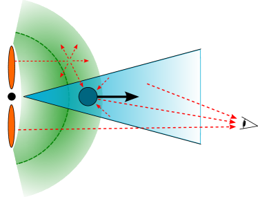
Figure 1: Left: Scheme of the Bjet model, dashed lines show the considered radiative transfers. Right: Example of an application of the Bjet model on the SED of the blazar AP Librae (Hervet et al., 2015).

2 Motivations for Bjet_MCMC

As mentioned above, Bjet has been used in multiple papers since its first development in 2015 and has shown its capability in modeling various types of blazars (HBLs, IBLs, LBLs, FSRQs) and a radiogalaxy candidate (PKS 0625–354). The main purpose of the project Bjet_MCMC is to provide this tool to the scientific community through an open GitHub project. Users can have access to the full Bjet code and perform one-zone pure SSC, one-zone SSC with thermal nucleus interactions (EIC + pair absorption), and multi-SSC zones with thermal nucleus interactions (blob + jet + nucleus).

The second motivation was to make a tool that automatically fits the multiwavelength SEDs and which is user-friendly and computationally efficient. SSC models are notorious for being challenging for standard $\chi^{2}$ minimization methods. They have high dimensionalities, parameter degeneracies, local minima, and model-dependant parameter boundaries. To illustrate this last point, let’s consider the particle distribution spectrum within the blob, which is set in our model as a broken power law.

$$N_{e}(\gamma)=\left\{\begin{array}[]{ll}N_{e}^{(1)}\gamma^{-n_{1}}&\mathrm{for}~{}\gamma_{\mathrm{min}}\leqslant\gamma\leqslant\gamma_{\mathrm{brk}}\\ N_{e}^{(2)}\gamma^{-n_{2}}&\mathrm{for}~{}\gamma_{\mathrm{brk}}\leqslant\gamma\leqslant\gamma_{\mathrm{max}}\end{array}\right.,$$ (1)

with $\gamma_{\mathrm{min}}$, $\gamma_{\mathrm{brk}}$ and $\gamma_{\mathrm{max}}$, the Lorentz factors of the radiating particles a the minimum, break, and maximum of their distribution. In this equation, $N_{e}^{(2)}=N_{e}^{(1)}\gamma_{\rm{brk}}^{(n_{2}-n_{1})}$, and $N_{e}^{(1)}$ the particle density factor set as $N_{e}^{(1)}=N_{e}(1)$.

Keeping free $\gamma_{\mathrm{min}}$, $\gamma_{\mathrm{brk}}$ and $\gamma_{\mathrm{max}}$ in a standard $\chi^{2}$ minimization algorithm will certainly create issues since the following condition $\gamma_{\mathrm{min}}<\gamma_{\mathrm{brk}}<\gamma_{\mathrm{max}}$ has to be respected. These constraints let us consider Markov-Chain Monte-Carlo (MCMC) methods as the most suited to perform a SED fit and explore the parameter space. Indeed, MCMCs have the advantage of building the best solution from posterior probability distributions, which is by default less impacted by discontinuity or non-linearity of the parameter space. We note here that this MCMC fitting approach of SSC models is relatively known in the community and has been implemented and used in multiple studies (e.g. Tramacere et al., 2011; Zabalza, 2015; Qin et al., 2018; Jiménez-Fernández & van Eerten, 2021)

In this paper, we do not intend to describe the general statistical concepts behind the MCMC methods. The literature on the subject is quite vast, we can recommend MacKay (2003), for example.

3 Implementing the MCMC method

For our project, we used the MCMC emcee package, which is a handy Python tool allowing a relatively simple implementation (Foreman-Mackey et al., 2013). emcee requires a user-defined probability function to evaluate the goodness of a fit. It then automatically builds the posterior probability density function following a given number of steps, walkers, and a defined burning sample. There are multiple flavors available on what type of move a walker can do on the parameter space, we use the default “StretchMove,” developed by Goodman & Weare (2010). A few other moves – or combinations of moves – were tested but did not display significant improvements compared to the proposed default method.

3.1 Probability function and free parameters

Our probability function is based on the $\chi^{2}$ value of the model on all considered SED spectral points. Asymmetric error bars are fully implemented in our $\chi^{2}$ calculation. We highlight here that flux upper limits are not considered in the fit, but can still be included in the input SED data file for display purposes only. A general advice is to merge constraining upper limits together into larger energy bins until we have a statistically significant data point before fitting the SED. As the emcee package requires a log probability, our probability function is defined as $\ln P=-\chi^{2}/2$.

The MCMC method is implemented for the single-zone SSC + thermal EIC model (blob + accretion disk + BLR). It includes up to 13 free parameters, as detailed in the sections below. The full Bjet model currently has 23 free parameters when including the SSC jet. We quickly realized that the computation time required to fit the full multi-zone model is not reasonable for user-friendly usage. In Bjet_MCMC, the user can decide to fix or free any of the 13 parameters. For pure SSC model fit, the user can deactivate the EIC option to save computation time.

3.2 Defining the $1\sigma$ parameter space and contour on the SED

The posterior distribution of probability allows us to define the parameter range corresponding to the $1\sigma$ confidence level ($\sim 68\%$) around the best solution. We follow the general solution proposed by Lampton et al. (1976); Avni (1976) based on the $\chi^{2}$ cumulative distribution function $\chi^{2}_{\mathrm{cdf}}$, or more precisely on the percent point function $\chi^{2}_{\mathrm{ppf}}$ which returns the $\chi^{2}$ value associated with a probability $P$ and a number of degrees of freedom $k$ of the $\chi^{2}_{\mathrm{cdf}}$. In this approach, we consider all models which have $\chi^{2}<\chi^{2}_{\mathrm{min}}+\Delta\chi^{2}$ as within $1\sigma$ of the best value, where $\chi^{2}_{\mathrm{min}}$ is our best solution and $\Delta\chi^{2}=\chi^{2}_{\mathrm{ppf}}(0.682,k)$. $k$ is the number of free parameters in our model that can range from 1 to 13.

Bjet_MCMC draws the $1\sigma$ contour in the SED associated with the parameter uncertainties. Solutions to get the exact contours were ruled out as too computing and disk-space demanding. For example, one can save all SED points for all models tested during the MCMC process, or run through thousands of randomly picked models within the $1\sigma$ parameter space. In order to save computation time, this contour is built by picking up models with extremum parameter values at the $1\sigma$ confidence level. We call it the “min-max method.” This allows us to build relatively good contours by re-running the code Bjet only twice the number of free parameters, which typically takes up to a few minutes with all 13 parameters free. Hence we must warn the user that the contours on the SED plots are an approximation and do not extend to the full theoretical space covered by the parameters uncertainties.

3.3 Parameters boundaries

The pure SSC model has 9 free parameters by default, in addition to 3 fixed parameters:

• The redshift $z$ is set by the user.

• The cosmology is set by default as a flat $\Lambda$CDM with H0 = 69.6 km s^-1 Mpc^-1, $\Omega M$ = 0.286, and $\Omega\Lambda$ = 0.714 (Bennett et al., 2014).

• The angle between the jet direction and the observer line of sight $\theta$ is fixed at 0.57 degrees to satisfy the Doppler boosted regime $\delta\sin{\theta}<1$, with the Doppler factor $\delta\leqslant 100$.

Table 1: Parameters and bounds.

	Range	Description	Scale
SSC Blob
$\delta$	[1 , 100]+	Doppler factor	linear
$N_{e}^{(1)}$	[0 , 8]	particle density factor [cm-3]	log10
$n_{1}$	[1 , 5]+	first index	linear
$n_{2}$	[1.5 , 7.5]+	second index	linear
$\gamma_{\mathrm{min}}$	[0 , 5]+	low-energy cutoff	log10
$\gamma_{\mathrm{max}}$	[3 , 8]+	high-energy cutoff	log10
$\gamma_{\mathrm{break}}$	[2 , 7]+	energy break	log10
$B$	[-4 , 0]	magnetic field strength [G]	log10
$R$	[14 , 19]+	blob radius [cm]	log10
Additional parameters for thermal EIC
$T_{\mathrm{disk}}$	[3.5 , 6]	disk temperature [K]	log10
$L_{\mathrm{disk}}$	[40 , 50]	disk luminosity [erg/s]	log10
$\epsilon_{\mathrm{BLR}}$	[-5 , 0]	covering factor of the BLR	log10
$D_{\mathrm{BH}}$*	[15 , 21]+	Distance blob - SMBH [cm]	log10
* Host galaxy frame.
+ Parameters with additional constraints.

In the MCMC implementation, we set minimum and maximum values for each of the parameters, as shown in Table 1. We intentionally use wide ranges for parameters to make as few assumptions as possible. Many parameters are in log scale to ease walkers’ moves through multiple orders of magnitude.

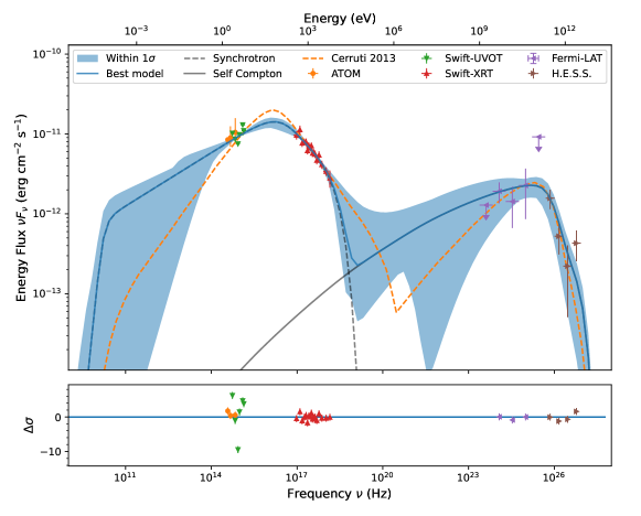
Figure 2: Results of Bjet_MCMC on the SED fit of the blazar 1RXS J101015.9-311909. The model applied was a one-zone pure SSC, including a gamma-ray EBL absorption following the model of Franceschini & Rodighiero (2017). The SED data points have been shared by the authors of Cerruti et al. (2013), while their model line itself has been manually digitized from the original paper.

Within our MCMC method, parameter boundaries mean that the posterior probability $\ln{P}=0$ for the fit with any parameter outside the given parameter range. The MCMC algorithm acts as an acceptance/reject method only based on the change of the posterior probability value from one walker step to the other. If a walker moves outside the parameter range, the move will be automatically rejected and the walker will try again. From the emcee package, a good acceptance rate is about 0.2. Given the additional parameter constraints developed below, Bjet_MCMC shows an acceptance rate in the order of $\sim 0.05-0.1$ from previous tests.

As highlighted in Table 1, multiple parameters have fluctuating boundaries intertwined with other parameter values. The particle spectrum, for example, must follow the condition of $\gamma_{\mathrm{min}}<\gamma_{\mathrm{brk}}<\gamma_{\mathrm{max}}$, and $n_{2}>n_{1}$. The fastest observed variability $\Delta t_{\mathrm{obs,min}}$ is also used to constrain the Doppler factor and size of the emitting region. From the simple argument that in the jet frame, the fastest variation cannot happen faster than the time the light takes to cross the blob radius, we apply the condition $R\leq{c\delta\Delta t_{\mathrm{obs,min}}}/(1+z)$. Finally, a last condition is applied, specifying that the blob diameter cannot be larger than the jet cross-section. From a radio study of a large sample of blazars, it can be noted that the intrinsic jet half-opening angle $\alpha_{\mathrm{jet}/2}$ is no more than 5 degrees. (e.g. Hervet et al., 2016). Using this conical jet approximation we set the condition $\alpha_{\mathrm{jet}/2}=\arctan(R/D_{\mathrm{BH}})180/\pi<5$.

4 Pure SSC validation on the HBL 1RXS J101015.9-311909

Table 2: Best fit and parameter comparison for 1RXS J101015.9-311909

	Cerruti et al. 2013		Bjet_MCMC
Parameter	Best Value	$1\sigma$ Range	Best Value	$1\sigma$ Range
$\delta$	96.83	32.07–99.53	83.8	35.8 – 100
$N_{e}^{(1)}$ [cm-3]	undefined	undefined	4.24$\times 10^{3}$	2.18$\times 10^{2}$ – $1.0\times 10^{6}$
$n_{1}$	2.0	fixed	2.56	2.31 – 2.74
$n_{2}$	4.0	fixed	3.75	3.25 – 4.24
$\gamma_{min}$	100	fixed	9.22	1.00 – $1.49\times 10^{4}$
$\gamma_{max}$	5$\times 10^{6}$	fixed	1.99$\times 10^{6}$	2.57$\times 10^{5}$ – 9.99$\times 10^{7}$
$\gamma_{break}$	5.31$\times 10^{4}$	(3.48–13.15)$\times 10^{4}$	2.13$\times 10^{5}$	2.40$\times 10^{4}$ – 3.93$\times 10^{5}$
$B$ [G]	0.015	(0.51 – 4.089)$\times 10^{-2}$	1.71$\times 10^{-3}$	7.92$\times 10^{-4}$ – 1.42$\times 10^{-1}$
$R$ [cm]	1.3$\times 10^{16}$	(0.49–11.57)$\times 10^{16}$	1.40$\times 10^{17}$	1.71$\times 10^{15}$ – 2.21$\times 10^{17}$
$\chi^{2}_{\mathrm{red}}$ total	260.6/27 = 9.65		187.1/24= 7.80
$\chi^{2}_{\mathrm{red}}$ X-ray – $\gamma$-ray	18.6/18 = 1.04		15.0/15= 1.00

The blazar 1RXS J101015.9-311900 is a high-frequency peaked BL Lac (HBL) with a redshift of $z=0.143$ that has been discovered emitting up to a few TeV by the H.E.S.S. Collaboration after an observing campaign between 2006 and 2010 (H.E.S.S. Collaboration et al., 2012). The multiwavelength SED of this source has been successfully fitted with a one-zone SSC model by Cerruti et al. (2013). In their study, they developed a fitting algorithm that relies on a strong parametrization of the SED features such as slopes and peaks, and extended the approach made by Tavecchio et al. (1998). They also probed the parameter space of their SSC model by discretizing it in a grid, each free parameter is divided into 10 points, with the exception of the particle index $n_{1}$ in only 3 points. This kind of probing method quickly becomes very computationally heavy for large dimensionality and has only 6 parameters that can be considered free to mitigate the computation time. On these parameters, they used a different definition of the blob density, which does not allow a straightforward comparison with our results.

Nevertheless, this multiwavelength SED is ideal for a validation test of Bjet_MCM and allows a partial comparison of results with the work of Cerruti et al. (2013). For this model, we considered 100 walkers, 5000 steps, and a burning phase of 200 steps. We ran it over 15 parallelized threads over a full time of 5h 45min. First, we can visually compare the two models on Figure 2. We see notable differences but a relatively equally good fit at first glance. We however achieved a better $\chi^{2}_{\mathrm{red}}$ considering the full dataset, or only the X-ray to gamma-ray dataset as used by Cerruti et al. (2013). These values are reported in Table 3. We observe a good agreement within errors on our free parameters. A notable difference is that the best value found of $n_{1}$ with Bjet_MCMC is outside the probed parameter range of Cerruti et al. (2013). Overall this comparison fully validates our approach for single-zone pure SSC models by providing to date the best SED fit and parameter characterization on the blazar 1RXS J101015.9-311909.

5 Fitting the FSRQ PKS 1222+216 with SSC + thermal EIC

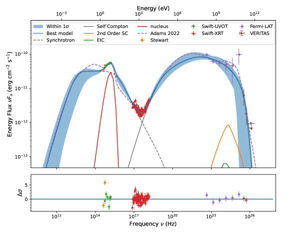
Figure 3: Results of Bjet_MCMC on the SED fit of the blazar PKS 1222+216. The model applied was a one-zone SSC + thermal EIC from the disk and BLR radiative interaction, including a gamma-ray EBL absorption by the model of Franceschini & Rodighiero (2017). The SED data points have been shared by the authors of Adams et al. (2022), while their model line itself has been manually digitized from the original paper.

Table 3: Best fit and parameter comparison for PKS 1222+216

	Adams et al. 2022	Bjet_MCMC
Parameter	Best Value	Best Value	$1\sigma$ Range
$\delta$	40	31.5	26.0 – 42.3
$N_{e}^{(1)}$ [cm-3]	2.0$\times 10^{4}$	1.12$\times 10^{7}$	3.41$\times 10^{5}$ – $9.97\times 10^{7}$
$n_{1}$	2.1	2.98	2.51 – 3.12
$n_{2}$	3.9	4.45	4.14 – 4.83
$\gamma_{min}$	$5.5\times 10^{2}$	$7.94\times 10^{2}$	$(3.43-9.51)\times 10^{2}$
$\gamma_{max}$	3.0$\times 10^{5}$	5.15$\times 10^{6}$	9.42$\times 10^{4}$ – 9.96$\times 10^{8}$
$\gamma_{break}$	5.0$\times 10^{3}$	3.09$\times 10^{4}$	4.40$\times 10^{3}$ - 5.22$\times 10^{4}$
$B$ [G]	3.0$\times 10^{-2}$	3.92$\times 10^{-2}$	1.25$\times 10^{-2}$ – 8.06$\times 10^{-1}$
$R$ [cm]	5.5$\times 10^{16}$	7.10$\times 10^{16}$	1.94$\times 10^{15}$ – 1.99$\times 10^{17}$
$T_{\mathrm{disk}}$ [K]	2.8$\times 10^{4}$	2.7$\times 10^{4}$	$(2.23-3.35)\times 10^{4}$
$L_{\mathrm{disk}}$ [erg s-1]	2.8$\times 10^{46}$	2.8$\times 10^{46}$	fixed
$\epsilon_{\mathrm{BLR}}$	2.0$\times 10^{-2}$*	2.0$\times 10^{-2}$	fixed
$D_{\mathrm{BH}}$ [cm]	1.10$\times 10^{19}$	4.56$\times 10^{19}$	$2.96\times 10^{18}-1.00\times 10^{21}$
$\chi^{2}_{\mathrm{red}}$	197.5/66 = 3.04	138.6/67 = 2.07

In order to further display the capabilities of Bjet_MCMC, we performed a test on the FSRQ PKS 1222+216 (z = 0.432), which is known to display bright gamma-ray outbursts (e.g. Tavecchio et al., 2011; Adams et al., 2022). It has been noticed that this blazar was a good candidate for SSC + thermal EIC models as EIC was proposed as the main source of VHE gamma-rays. However, without a proper fitting method, it is challenging to fully discard the one-zone pure SSC. This point may actually be the most critical in the relevance of Bjet_MCMC as it is to date likely the first public code that can provide a fit with a full SSC+EIC model (13 free parameters). As pure SSC and SSC+EIC models are nested, Bjet_MCMC can provide a statistical test that allows to reject the pure SSC hypothesis.

It has to be noted that MCMC methods can still struggle in complicated parameter spaces and be stuck in local minima. Eventually, a proper MCMC algorithm should always end up in the real best solution. The computation time needed can however be unachievable with standard computers.

In this section, we compare the results of Bjet_MCMC on the 2014 flare SED of PKS 1222+216 published by Adams et al. (2022). In their paper, the SED model was manually crafted through a “fit by eye” model using Bjet. Being fitted with the same core code (with only minor updates since then), we can have a proper parameter-by-parameter check on how the results of Bjet_MCMC differ from the previous model.

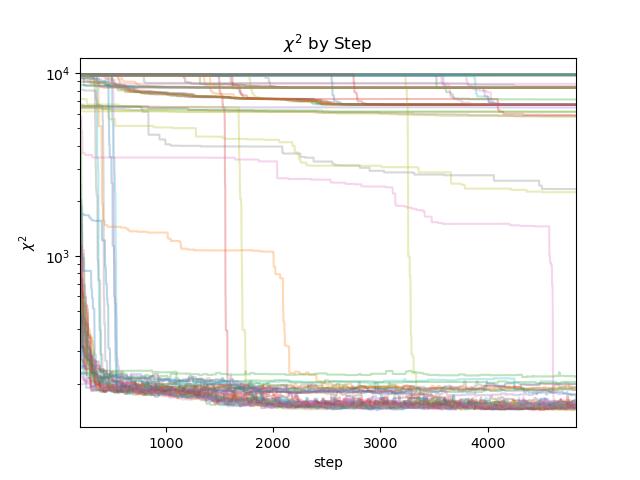
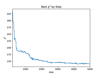
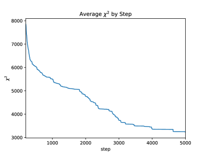
Figure 6: Bjet_MCMC $\chi^{2}$ values of walkers at each step for the SED fit of PKS 1222+216. Upper-left: all walkers, Upper-right: smallest $\chi^{2}$, Bottom: average $\chi^{2}$.

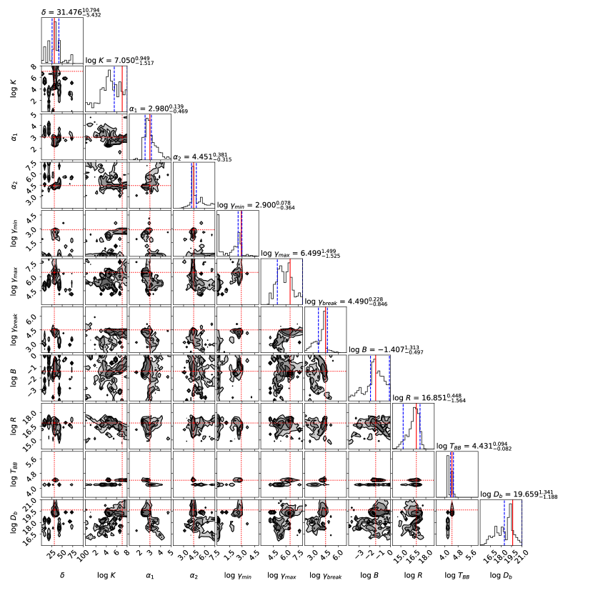
Figure 7: Corner plot of the posterior probability distribution of the free parameters from the SED fit of PKS 1222+216.

For this fit, we used the same MCMC setup as for 1RXS J101015.9-311900 (100 walkers, 5000 steps, 200 steps of burning phase, 15 computing threads). Activating the interaction with the thermal nucleus emission significantly increases the computation time for each step. The full MCMC chain took a total of 12h to run. After noticing multiple $\chi^{2}$ local minima, we fixed two parameters to the Adams et al. (2022) value which are the BLR covering factor $\epsilon_{\mathrm{BLR}}=1\times 10^{-2}$ and the accretion disk luminosity $L_{\mathrm{disk}}=2.8\times 10^{46}$ erg s^-1. As seen in Figure 3, the best fit is visually convincing. We also observe in Figure 6 that the MCMC walkers display a good general $\chi^{2}$ convergence. However, we still have hints of local minima, such as in Figure 6, Top-left, where a small fraction of walkers get stuck away from the best fit. They also appear as “islands” in the parameter space corner plot (see Figure 7).

Results of Bjet_MCMC show better fit $\chi^{2}$ compared to the model of Adams et al. (2022). It is interesting to notice that the best solution of Bjet_MCMC does not favor any significant contribution for EIC emission in gamma rays. However, it does not rule out a strong EIC emission either. In the study of Adams et al. (2022), it was estimated that the distance to the SMBH should be at least about one parsec to avoid too much gamma-gamma absorption from the BLR. This is relatively consistent with the estimated distance of $D_{\mathrm{BH}}$ from our fit which is found at above 0.96 pc from the SMBH.

6 Computational performances and general using advice

Bjet_MCMC makes full use of the paralellized capability of the emcee package. By running several tests, we observed a roughly linear improvement in the computation time following the number of parallel threads used for the fitting process. We have not performed extensive testing to check if this linear relation was holding true at more than about a dozen of threads. It is expected that I/O processes will diminish the relevance of large parallelization at some point. We recommend using a large number of computing threads if available, likely at least 4 for the pure SSC and at least 15 for SSC+EIC if a user wants to get results overnight. Bjet_MCMC will be the most relevant if used in a computing center with several tens of available computing threads.

6.1 Quality checks and length of MCMC chains

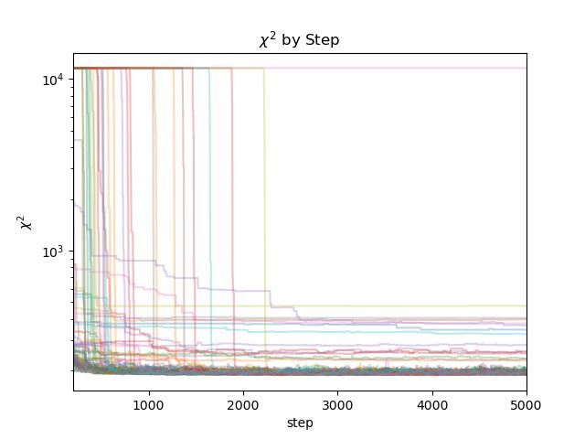
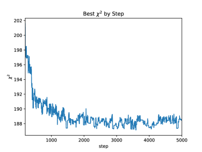
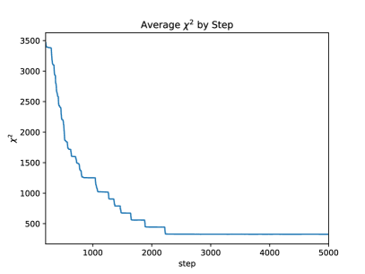
Figure 4: Bjet_MCMC $\chi^{2}$ values of walkers at each step for the SED fit of 1RXS J101015.9-311900. Upper-left: all walkers, Upper-right: smallest $\chi^{2}$, Bottom: average $\chi^{2}$.

We propose a few ways to estimate if a user gets enough walkers and steps to be confident in the output of Bjet_MCMC, with some warnings and advice. The favored test to check if the fit is optimal is to get a look at the “average $\chi^{2}$ per step” plot. For example, one can see in Figure 4 for 1RXS J101015.9-311909 that the average $\chi^{2}$ plateaued at about 2500 steps. We can confidently deduce that only 3000 steps would have been enough for this fit as no further improvements are observed afterward. Now looking at the same plot from PKS 1222+216 in Figure 6, we observe a good convergence of the average $\chi^{2}$ but not a full plateauing yet. This means that the full extent of the 1-sigma parameter space is likely going to change marginally. This is usually not a big issue, but one should avoid drawing too firm a conclusion from the exact number of the error associated with parameters. A good practice would be to add an extra 20% on the parameter errors to get a more conservative parameter range when the average $\chi^{2}$ curve does not fully flatten out. If the average $\chi^{2}$ curve does not show any sign of asymptotical behavior, then the number of steps and/or walkers needs to be increased.

Note that the best $\chi^{2}$ always converges faster than the average $\chi^{2}$ (see Figures 4, 6). The best $\chi^{2}$ convergence gives a confidence estimation on the best model while the average $\chi^{2}$ convergence gives a confidence estimation of the associated parameter errors. The plot “$\chi^{2}$ per step” gives a view of the entirety of walkers. It is a relatively efficient way of checking for local $\chi^{2}$ minima in the parameter space. As soon as most walkers converge toward the best solution, this should not have significant consequences in the results. If most of the walkers appear to be stuck in local minima, then your SED dataset is not constraining enough for the complexity of the model. You can run a longer chain to hope for the MCMC method to eventually converge, or reduce the model complexity by freezing parameters.

emcee considers unsafe a number of steps fewer than 50 times the integrated autocorrelation time $\tau_{\mathrm{corr}}$ (in steps). We find this boundary challenging to achieve in most of our tests, but also not systematically leading to better results when met. The value $\tau_{\mathrm{corr}}$ is given as an output of Bjet_MCMC. We generally advise a safe boundary of $n_{\mathrm{steps}}\geq 10\tau_{\mathrm{corr}}$. However, a general check on the $\chi^{2}$ convergence plots and a visual check on the SED itself should always be given to assess the fit quality.

6.2 Advice in building a MWL SED

Blazars showing great variability should be treated with caution when building their MWL SED. Bjet_MCMC is a stationary model, which means that within the period considered for the SED, we assume an equilibrium between particle injection and cooling mechanisms. The code cannot model any flux variation or describe any time lags between flares observed at different energies. It is possible to model the SED of a flare with Bjet_MCMC, such as PKS 1222+216 in Fig. 3, but we need to ensure that the time period used for modeling can be considered as steady. It is done, for example, by using a time period much smaller than the duration of the flare. Longer integration times are often used for lower-sensitivity instruments, and non-simultaneous datasets are often used to build a more detailed SED. There is no single way of building a MWL SED since most of the time, it consists of finding the best trade-off between data quantity and quality. In any case, datasets, time periods, and assumptions used to build SEDs should be documented by users of Bjet_MCMC. The modeling results are as relevant as the prior assumptions used to build a SED.

Some spectral points with very small errors may be overconstraining the fit to the detriment of another energy range. For example, a 10% model flux variation in optical may be as constraining as a factor 2 for gamma rays. From a statistical point of view, this is exactly how we expect the fit to behave following the error bars of spectral points. However, the flux “real” errors are often widely underestimated in low energies. The error in each spectral point should reflect the flux variations during the integration period used to build the SED. We advise users to use the RMS error of flux variation instead of the statistical error of individual observations, when larger. It appears that both optical SEDs used in this paper likely have overconstraining error bars.

6.3 Other considerations

A full version of the multi-zone Bjet code is available to be used through the package Bjet_MCMC, but contains a full amount of 23 free parameters, and consequently is not included in the MCMC method. The multi-zone model is recommended to be used only by scientists who have a deep knowledge of blazar emission models as there are significant risks of having an inconsistent or unphysical set of parameters. This risk has been mitigated for the pure SSC and SSC+EIC models through parameter constraints, but the final assessment of interpreting the quality and relevance of Bjet_MCMC results is the responsibility of the user.

7 Conclusion

Bjet_MCMC is a new tool in the growing family of SSC models of blazars. Its full version includes 2 SSC zones + EIC, based on Hervet et al. (2015). However, only the one-zone pure SSC and one-zone SSC+EIC are fully implemented in the automatic MCMC fitting method. Bjet_MCMC is aimed to be a user-friendly tool that only requires minimal input from the user, namely a configuration file and a SED data file. It is fully parallelized and can take advantage of computing clusters. The code works as intended and produces consistent results. There are other publicly available SSC models at this time that contain SED fitting algorithms. Among the most known are AGNpy (Nigro et al., 2022), JetSet (Tramacere et al., 2011), and Naima (Zabalza, 2015). We do not provide any comparison between Bjet_MCMC and these models in terms of consistency of results, performances, and capabilities. This will be addressed in further studies. However, it has to be noted that Bjet_MCMC appears to be at the current time the only public tool with an automatic fitting that can handle a full SSC+EIC model with up to 13 free parameters. It needs to be noted that excellent broadband energy coverage of the SED has to be built in order to obtain a good convergence of all parameters for the most extensive model version. This tool needs the user to have some knowledge of the blazar emission processes to understand the limits of SSC models and infer scientific interpretation from their outputs. Finally, we highlight that the model is still having frequent updates, and some information mentioned in this paper may be quickly outdated. One of our priorities is to explore routes to reduce further the computation time, such as reducing I/O and further optimizing the energy discretization of the radiative components. The most updated version with relevant information is available publicly on Github.

Appendix A Additional Bjet_MCMC outputs for 1RXS J101015.9-311900

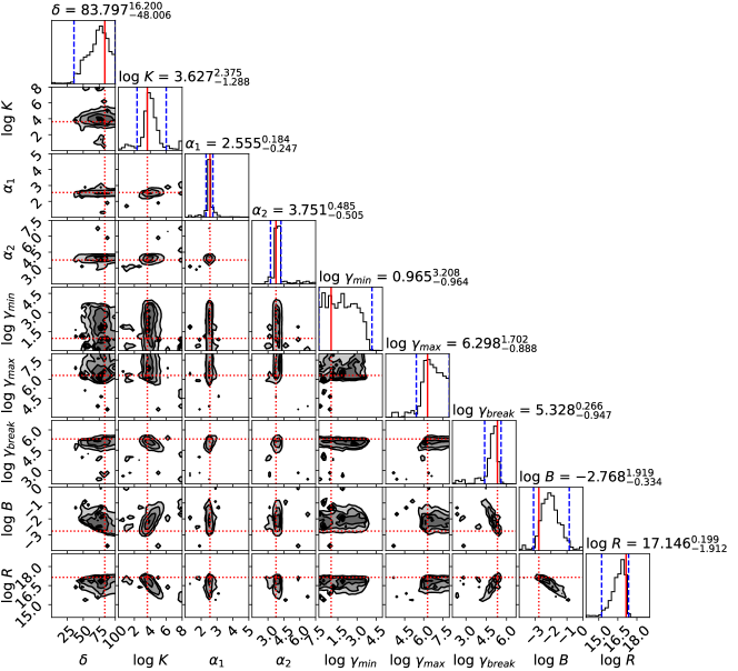
Figure 5: Corner plot of the posterior probability distribution of the free parameters from the SED fit of 1RXS J101015.9-311900.

Appendix B Additional Bjet_MCMC outputs for PKS 1222+216

References

- Adams et al. (2022) Adams, C. B., Batshoun, J., Benbow, W., et al. 2022, ApJ, 924, 95, doi: 10.3847/1538-4357/ac32bd
- Archer et al. (2018) Archer, A., Benbow, W., Bird, R., et al. 2018, ApJ, 862, 41, doi: 10.3847/1538-4357/aacbd0
- Astropy Collaboration et al. (2013) Astropy Collaboration, Robitaille, T. P., Tollerud, E. J., et al. 2013, A&A, 558, A33, doi: 10.1051/0004-6361/201322068
- Avni (1976) Avni, Y. 1976, ApJ, 210, 642, doi: 10.1086/154870
- Bennett et al. (2014) Bennett, C. L., Larson, D., Weiland, J. L., & Hinshaw, G. 2014, ApJ, 794, 135, doi: 10.1088/0004-637X/794/2/135
- Cerruti et al. (2013) Cerruti, M., Boisson, C., & Zech, A. 2013, A&A, 558, A47, doi: 10.1051/0004-6361/201220963
- Foreman-Mackey et al. (2013) Foreman-Mackey, D., Hogg, D. W., Lang, D., & Goodman, J. 2013, PASP, 125, 306, doi: 10.1086/670067
- Franceschini & Rodighiero (2017) Franceschini, A., & Rodighiero, G. 2017, A&A, 603, A34, doi: 10.1051/0004-6361/201629684
- Ghisellini & Madau (1996) Ghisellini, G., & Madau, P. 1996, MNRAS, 280, 67, doi: 10.1093/mnras/280.1.67
- Ghisellini et al. (1985) Ghisellini, G., Maraschi, L., & Treves, A. 1985, A&A, 146, 204
- Ghisellini et al. (2005) Ghisellini, G., Tavecchio, F., & Chiaberge, M. 2005, A&A, 432, 401, doi: 10.1051/0004-6361:20041404
- Ginzburg & Syrovatskii (1965) Ginzburg, V. L., & Syrovatskii, S. I. 1965, ARA&A, 3, 297, doi: 10.1146/annurev.aa.03.090165.001501
- Ginzburg & Syrovatskii (1969) —. 1969, ARA&A, 7, 375, doi: 10.1146/annurev.aa.07.090169.002111
- Goodman & Weare (2010) Goodman, J., & Weare, J. 2010, Communications in Applied Mathematics and Computational Science, 5, 65, doi: 10.2140/camcos.2010.5.65
- Gould (1979) Gould, R. J. 1979, A&A, 76, 306
- Hervet (2015) Hervet, O. 2015, Theses, Observatoire de paris. https://hal.science/tel-01240215
- Hervet et al. (2015) Hervet, O., Boisson, C., & Sol, H. 2015, A&A, 578, A69, doi: 10.1051/0004-6361/201425330
- Hervet et al. (2016) —. 2016, A&A, 592, A22, doi: 10.1051/0004-6361/201628117
- H.E.S.S. Collaboration et al. (2012) H.E.S.S. Collaboration, Abramowski, A., Acero, F., et al. 2012, A&A, 542, A94, doi: 10.1051/0004-6361/201218910
- HESS Collaboration et al. (2018) HESS Collaboration, Abdalla, H., Abramowski, A., et al. 2018, MNRAS, 476, 4187, doi: 10.1093/mnras/sty439
- Hunter (2007) Hunter, J. D. 2007, Computing in Science & Engineering, 9, 90, doi: 10.1109/MCSE.2007.55
- Inoue & Takahara (1996) Inoue, S., & Takahara, F. 1996, ApJ, 463, 555, doi: 10.1086/177270
- Jiménez-Fernández & van Eerten (2021) Jiménez-Fernández, B., & van Eerten, H. J. 2021, MNRAS, 500, 3613, doi: 10.1093/mnras/staa3163
- Jones et al. (2001–) Jones, E., Oliphant, T., Peterson, P., et al. 2001–, SciPy: Open source scientific tools for Python. http://www.scipy.org/
- Katarzyński et al. (2001) Katarzyński, K., Sol, H., & Kus, A. 2001, A&A, 367, 809, doi: 10.1051/0004-6361:20000538
- Lampton et al. (1976) Lampton, M., Margon, B., & Bowyer, S. 1976, ApJ, 208, 177, doi: 10.1086/154592
- Longair (1994) Longair, M. S. 1994, High energy astrophysics. Vol.2: Stars, the galaxy and the interstellar medium, Vol. 2
- MacKay (2003) MacKay, D. J. C. 2003, Information Theory, Inference, and Learning Algorithms (Cambridge University Press). http://www.cambridge.org/0521642981
- Maraschi & Rovetti (1994) Maraschi, L., & Rovetti, F. 1994, ApJ, 436, 79, doi: 10.1086/174882
- Marscher (1980) Marscher, A. P. 1980, ApJ, 235, 386, doi: 10.1086/157642
- Marscher & Gear (1985) Marscher, A. P., & Gear, W. K. 1985, ApJ, 298, 114, doi: 10.1086/163592
- Nalewajko et al. (2014) Nalewajko, K., Begelman, M. C., & Sikora, M. 2014, ApJ, 789, 161, doi: 10.1088/0004-637X/789/2/161
- Nigro et al. (2022) Nigro, C., Sitarek, J., Gliwny, P., et al. 2022, A&A, 660, A18, doi: 10.1051/0004-6361/202142000
- Padovani & Giommi (1995) Padovani, P., & Giommi, P. 1995, ApJ, 444, 567, doi: 10.1086/175631
- Qin et al. (2018) Qin, L., Wang, J., Yang, C., et al. 2018, PASJ, 70, 5, doi: 10.1093/pasj/psx150
- Sikora et al. (1994) Sikora, M., Begelman, M. C., & Rees, M. J. 1994, ApJ, 421, 153, doi: 10.1086/173633
- Tavecchio et al. (2011) Tavecchio, F., Becerra-Gonzalez, J., Ghisellini, G., et al. 2011, A&A, 534, A86, doi: 10.1051/0004-6361/201117204
- Tavecchio et al. (1998) Tavecchio, F., Maraschi, L., & Ghisellini, G. 1998, ApJ, 509, 608, doi: 10.1086/306526
- Tramacere et al. (2011) Tramacere, A., Massaro, E., & Taylor, A. M. 2011, ApJ, 739, 66, doi: 10.1088/0004-637X/739/2/66
- Urry & Padovani (1995) Urry, C. M., & Padovani, P. 1995, PASP, 107, 803, doi: 10.1086/133630
- Valverde et al. (2020) Valverde, J., Horan, D., Bernard, D., et al. 2020, ApJ, 891, 170, doi: 10.3847/1538-4357/ab765d
- Walt et al. (2011) Walt, S. v. d., Colbert, S. C., & Varoquaux, G. 2011, Computing in Science & Engineering, 13, 22, doi: 10.1109/MCSE.2011.37
- Zabalza (2015) Zabalza, V. 2015, Proc. of International Cosmic Ray Conference 2015, 922