11institutetext: Instituto de Física Teórica UAM/CSIC, Calle Nicolás Cabrera 13-15, 28049 Madrid, Spain22institutetext: Departamento de Física Teórica, Universidad Autónoma de Madrid, Campus de Cantoblanco, 28049 Madrid, Spain

Pseudospectra of Holographic Quasinormal Modes

Daniel Areán 1,2    David García Fariña 1    Karl Landsteiner daniel.arean@uam.es david.garciafarinna@estudiante.uam.es karl.landsteiner@csic.es
Abstract

Quasinormal modes and frequencies are the eigenvectors and eigenvalues of a non-Hermitian differential operator. They hold crucial significance in the physics of black holes. The analysis of quasinormal modes of black holes in asymptotically Anti-de Sitter geometries plays also a key role in the study of strongly coupled quantum many-body systems via gauge/gravity duality. In contrast to normal Sturm-Liouville operators, the eigenvalues of non-Hermitian (and non-normal) operators generally exhibit instability under small perturbations. This research focuses on the stability analysis of quasinormal frequencies pertaining to asymptotically planar AdS black holes, employing pseudospectrum analysis. Specifically, we concentrate on the pseudospectra of scalar and transverse gauge fields, shedding light on their relevance within the framework of gauge/gravity duality.

preprint: IFT-UAM/CSIC-23-091

1 Introduction

Quasinormal modes are the solutions of linear differential equations on an open domain. The openness is encoded in outgoing boundary conditions. Such boundary conditions arise naturally in many branches of physics from the study of black holes to optics. The quasinormal modes can be thought of as the eigenmodes of linear differential operators. Due to the open boundary conditions the differential operator is non-Hermitian and the eigenvalues are complex.

In gravitational physics, quasinormal modes are of utmost importance in the theory of black holes. Famously, a black hole horizon acts as a perfectly absorbing membrane. Therefore, solving a wave equation in a black hole background leads naturally to outgoing boundary conditions. In asymptotically flat space, radiation is also outgoing at infinity. The quasinormal modes that arise in asymptotically flat spacetimes are supposed to describe the late time ringdown of perturbed black holes. They arise for example in black hole mergers and are of highest interest for gravitational wave physics Nollert:1999ji ; Kokkotas:1999bd ; Berti:2009kk ; Franchini:2023eda .

The importance of quasinormal modes in asymptotically Anti de-Sitter (AdS) spaces derives from gauge/gravity duality Maldacena:1997re ; Aharony:1999ti ; BigJ ; zaanen2015holographic ; Hartnoll:2018xxg . Famously gauge/gravity duality is conjectured to describe certain strongly coupled quantum many-body systems. While up to date no concrete physical system has been found that indeed is modelled in all detail by gauge/gravity duality, it has lead to important insights into areas such as hydrodynamics and transport theory in the relativistic regime Policastro:2001yc ; Baier:2007ix ; Bhattacharyya:2007vjd . Some key results are the extremely low specific shear viscosity of holographic models of the quark gluon plasma Kovtun:2004de or phase transitions towards superconducting states Gubser:2008px ; Hartnoll:2008vx as well as strongly coupled quantum critical phases Herzog:2007ij . Quasinormal modes are a key ingredient in this development as they can be understood as the poles of the retarded Green’s functions of the strongly coupled quantum many-body system Horowitz:1999jd ; Birmingham:2001pj ; Kovtun:2005ev . The shear viscosity can be read off from a quasinormal mode corresponding to momentum diffusion Policastro:2002se1 and second order phase transitions arise as a quasinormal frequency moves into the upper half plane thus indicating an instability of the ground state Herzog:2009ci ; Amado:2009ts .

In particular the modern way of understanding relativistic hydrodynamics is very much influenced by the properties of quasinormal modes in asymptotically AdS black holes. Relativistic hydrodynamics can be understood as an effective field theory organised in a derivative expansion Kovtun:2012rj . As an effective field theory it has a limited range of validity. This limit can be set as the wavelength at which the first non-hydrodynamic modes decays at a slower rate than the hydrodynamic mode Amado:2008ji . More recently it is conjectured that the limit is set by the radius in the complex plane at which the lowest hydrodynamic quasinormal modes collide with the first non-hydrodynamic mode Withers:2018srf ; Grozdanov:2019 ; GrozdanovKovtun:2019 .

A question that so far has not been investigated in the context of gauge/gravity duality is the stability of the quasinormal frequencies under small perturbations of the background geometry. In asymptotically flat space such studies have a long history Nollert:1996rf ; Nollert:1998ys and recently the issue has been taken up in Jaramillo:2020tuu ; Destounis:2021lum ; Sarkar:2023rhp ; Cheung:2021bol ; Berti:2022xfj ; Konoplya:2022pbc ; Courty:2023rxk (see also Boyanov:2022ark for horizonless compact objects). The key new development of these recent studies is the application of the method of pseudospectra Trefethen:2005 .

The eigenvalues of Hermitian operators are stable in a technical sense. In fact, this stability is what makes perturbation theory successful in quantum physics. On the other hand, the eigenvalues of non-Hermitian and non-normal operators generically are unstable. This means they can be displaced large distances by even small perturbations of the original operator. Here stability and smallness of a perturbation have precise meanings and we will give exact definitions later on.

Concretely, in the case of quasinormal modes the instability appears as a consequence of the non-conservative nature of the system, associated with the eventual damping of the fluctuations as they fall into the black hole (and radiate away to infinite in asymptotically flat spacetime). AdS at large distances from the black hole horizon acts as a confining box but it is still true that fluctuations are damped as they fall into the black hole.

Thus the damping of fluctuations in black hole geometries is independent of the asymptotics of the spacetime. It is then reasonable to expect that such quasinormal modes and frequencies are also inherently unstable as occurs in asymptotically flat space. The motivation for investigating this question is twofold. Firstly, it would serve as increasing evidence of the independence of the instability on the asymptotic behaviour of the spacetime. And secondly, it would shed a completely new light on the behaviour of strongly coupled quantum many-body systems modelled by gauge/gravity duality. The instability of the quasinormal mode spectrum would indicate that also the excitation spectrum of the dual quantum field theories would be unstable under perturbations. In turn, this might rise questions about the robustness of conclusions for quantum many-body physics drawn from the behavior of quasinormal modes. Let us add here that despite the theoretically well established instability of the quasinormal mode spectrum in the asymptotically flat case, extraction of overtones from gravitational wave signals have been reported in Isi:2019aib ; Giesler:2019uxc ; Capano:2021etf ; Capano:2022zqm .

To probe the stability of the quasinormal mode frequency (QNF) we follow the example of Jaramillo:2020tuu and turn to pseudospectrum analysis Trefethen:2005 . Broadly speaking, pseudospectrum provides insight on how much perturbations of a given size can displace the spectrum of an operator. Accordingly, once the physically motivated notion of size is defined, pseudospectra serve as a powerful tool to discuss spectral stability or lack thereof.

In this work we initiate a systematic study of the stability of quasinormal frequencies in AdS. We focus on two very simple cases: a real scalar field and a transverse gauge field in a Schwarzschild AdS4+1 black brane (SAdS4+1). By the gauge gravity duality these correspond to a scalar operator and a conserved R𝑅R-current of the strongly coupled maximally symmetric 𝒩=4𝒩4\mathcal{N}=4 Yang-Mills theory Maldacena:1997re . Our choice of fluctuations is motivated by two main reasons. Firstly, we consider the SAdS4+1 background because it is the archetypical example for gauge/gravity duality. Secondly, we choose a real scalar and a transverse gauge field for their simplicity and their lack of a hydro mode. Hydro modes dominate the low energy spectrum of the dual QFT as their corresponding QNF goes to zero as the momentum goes to zero. Consequently, analyzing the stability of hydro modes is akin to studying the stability of the hydrodynamic description of the dual quantum field theory Kovtun:2005 . As the study of hydrodynamic modes involves additional technical complexities due to the presence of gauge symmetries and the corresponding constraints, we will leave this topic for a follow-up work.

The organisation of this paper is as follows. Since the method of pseudospectra is relatively new and perhaps little known in the context of gauge/gravity duality we spend the first few sections reviewing some of the underlying mathematics. Here we draw heavily from Trefethen:2005 and also from a previous work on asymptotically flat space Jaramillo:2020tuu . In particular we define the pseudospectrum and review its most important properties in section 2.

In section 3 we focus specifically on the application of pseudspectra to quasinormal modes. We point out the importance of chosing the proper coordinates. Following Warnick:2013hba we chose a coordinate slice which we call regular. These coordinates have the important property that the equal time slices are spacelike outside the horizon but coincide with infalling Eddington-Finkelstein coordinates at the horizon.111We note that infalling coordinates are very well suited to impose outgoing boundary conditions. We discuss the importance of the choice of norm and give a physical reasoning why the chosen energy norm is the relevant one in the holographic context. Indeed, the energy in regular coordinates is not conserved due to outflow on the horizon.

In section 4 we construct the specific differential operators that describe the fluctuations of scalar and transverse gauge fields in an AdS black hole background. We show explicitly that the non-Hermiticity is concentrated on the horizon. As we discuss in detail this leads to a clear picture of the local origin of the non-Hermiticity and non-normality.

In section 5 we first outline our numerical methods which are based on pseudospectral methods Trefethen:2000 ; boyd . Next, we introduce the selective pseudospectrum which tests the stability under random local potential perturbations. And finally, to further explore the aforementioned stability, we construct specific potentials to test some relevant regimes.

Section 6 is the core of the paper and contains the results of our pseudospectrum calculations. We mostly concentrate on the results for the energy norm but, to illustrate the norm dependence, we also present the result for the L2superscript𝐿2L^{2} norm in appendix C. Indeed it turns out that the pseudospectrum for both the scalar field and the transverse vector show the typical open contour lines indicating instability.

In section 7 we summarize our findings, present our conclusions and give an outlook on further studies in particular the highly interesting case of hydrodynamic modes.

Some of the more technical details on the calculation of the adjoint differential operators and the numerical methods are presented in the appendices A, B and E. The numerical values of the quasinormal frequencies are presented in appendix D.

2 Pseudospectrum and Stability

In this section we collect relevant theorems and definitions of the pseudospectrum of linear operators. We next specialize them to finite dimensional operators (matrices) and illustrate some key notions through the example of a 2×2222\times 2 matrix. For additional details, we refer the reader to Trefethen:2000 .

Given a closed linear operator L𝐿L acting on a Hilbert space \mathcal{H} with domain 𝒟(L)𝒟𝐿\mathcal{D}(L), its spectrum σ(L)𝜎𝐿\sigma\left(L\right) is defined as the set of points in the complex plane, z𝑧z, where its resolvent:222Recall that a closed linear operator L𝐿L is a linear operator such that if a sequence {xn}subscript𝑥𝑛\{x_{n}\} in \mathcal{H} converges to x𝑥x, then the sequence {Lxn}𝐿subscript𝑥𝑛\{Lx_{n}\} converges to y𝑦y, where Lx=y𝐿𝑥𝑦Lx=y. From now on, when talking about operators, we implicitly assume that they are both closed and linear.

(z;L)=(Lz)1,𝑧𝐿superscript𝐿𝑧1\displaystyle\mathcal{R}(z;L)=(L-z)^{-1}\,, (1)

does not exist as a bounded operator on \mathcal{H}.

Within σ(L)𝜎𝐿\sigma\left(L\right), we define the eigenvalues {λi}subscript𝜆𝑖\{\lambda_{i}\} through the eigenvalue equation:

Lui=λiui,𝐿subscript𝑢𝑖subscript𝜆𝑖subscript𝑢𝑖Lu_{i}=\lambda_{i}u_{i}\,, (2)

where ui𝒟(L)subscript𝑢𝑖𝒟𝐿u_{i}\in\mathcal{D}(L) is the eigenvector corresponding to the eigenvalue λisubscript𝜆𝑖\lambda_{i}. Note that with our definitions, the eigenvalues correspond to isolated points in the spectrum (regions of dimension 0). Nonetheless, it is important to stress that, in general, the spectrum also contains regions of higher dimension, such as branch cuts (regions of dimension 1). That said, Warnick:2013hba proved that in the case of Schwarzschild AdS black holes the spectrum of quasinormal frequencies indeed consists of isolated points.

A particularly important property of eigenvalues is that as long as the operator is self-adjoint (or, in more physical terms, the system is conservative), the spectral theorem ensures that if we perturb the system with a bounded operator of size ε𝜀\varepsilon the eigenvalues of the perturbed operator cannot suffer a displacement greater than ε𝜀\varepsilon kato2013perturbation ; Courant:1989 .333The notion of size here is quite nontrivial and we shall discuss it in greater detail later. In general, we will consider that the size is given by the norm of the operator, which is inherited from the function norm in \mathcal{H}. More generally, this property holds for any normal operator A𝐴A satisfying [A,A]=0𝐴superscript𝐴0\left[A,A^{\dagger}\right]=0, with Asuperscript𝐴A^{\dagger} the adjoint of A𝐴A. Physically, this ensures that any statement made relying on eigenvalue analysis is guaranteed to be right up to corrections of the same size as the error implicitly made when assuming a particular model.

However, many physical systems are inherently non-conservative. In these systems, normality of the relevant operators is not guaranteed and therefore eigenvalues are, in general, no longer protected by the spectral theorem; meaning that small perturbations could potentially alter the spectrum in a significant manner. As any description of a physical system is always a model and consequently has some inherent error associated with it, one can conclude Trefethen:2005 that eigenvalue analysis is insufficient when dealing with non-conservative systems defined through non-self-adjoint (and potentially non-normal) operators as eigenvalues may not be stable.

In order to characterize the stability of eigenvalues we need to introduce the notion of ε𝜀\varepsilon-pseudospectrum, which can be defined in three mathematically equivalent ways Trefethen:2005 :

Def. 2.1 (Resolvent norm approach).

Given a closed linear operator L𝐿L acting on a Hilbert space \mathcal{H} with domain 𝒟(L)𝒟𝐿\mathcal{D}(L), and ε>0𝜀0\varepsilon>0, the ε𝜀\varepsilon-pseudospectrum σε(L)subscript𝜎𝜀𝐿\sigma_{\varepsilon}(L) is

σε(L)={z:(z;L)>1/ε},subscript𝜎𝜀𝐿conditional-set𝑧delimited-∥∥𝑧𝐿1𝜀\sigma_{\varepsilon}(L)=\{z\in\mathbb{C}:\lVert\mathcal{R}(z;L)\rVert>1/\varepsilon\}\,, (3)

with the convention (z;L)=delimited-∥∥𝑧𝐿\lVert\mathcal{R}(z;L)\rVert=\infty for zσ(L)𝑧𝜎𝐿z\in\sigma(L).

Def. 2.2 (Perturbative approach).

Given a closed linear operator L𝐿L acting on a Hilbert space \mathcal{H} with domain 𝒟(L)𝒟𝐿\mathcal{D}(L), and ε>0𝜀0\varepsilon>0, the ε𝜀\varepsilon-pseudospectrum σε(L)subscript𝜎𝜀𝐿\sigma_{\varepsilon}(L) is

σε(L)={z,V,V<ε:zσ(L+V)}.\sigma_{\varepsilon}(L)=\{z\in\mathbb{C},\exists V,\rVert V\lVert<\varepsilon:z\in\sigma(L+V)\}\,. (4)
Def. 2.3 (Pseudoeigenvalue approach).

Given a closed linear operator L𝐿L acting on a Hilbert space \mathcal{H} with domain 𝒟(L)𝒟𝐿\mathcal{D}(L), and ε>0𝜀0\varepsilon>0, the ε𝜀\varepsilon-pseudospectrum σε(L)subscript𝜎𝜀𝐿\sigma_{\varepsilon}(L) is

σε(L)={z,uε𝒟(L):(Lz)uε<εuε},\sigma_{\varepsilon}(L)=\{z\in\mathbb{C},\exists u^{\varepsilon}\in\mathcal{D}(L):\;\rVert(L-z)u^{\varepsilon}\lVert<\varepsilon\lVert u^{\varepsilon}\rVert\}\,, (5)

where uεsuperscript𝑢𝜀u^{\varepsilon} is a ε𝜀\varepsilon-pseudoeigenvector with ε𝜀\varepsilon-pseudoeigenvalue z𝑧z.

Note that, contrary to the spectrum, the pseudospectrum depends on the operator norm as it needs a notion of what constitutes a large or small perturbation to quantify stability.

Def. 2.4 (Operator norm).

Given a bounded linear operator V𝑉V acting on a Hilbert space \mathcal{H} equipped with a function norm delimited-∥∥\lVert\cdot\rVert, we define its norm Vdelimited-∥∥𝑉\lVert V\rVert as:

V=maxuVuu.norm𝑉𝑢norm𝑉𝑢norm𝑢\norm{V}=\underset{u\in\mathcal{H}}{\max}\frac{\norm{Vu}}{\norm{u}}\,. (6)

Definition 2.2 corresponds to the physical intuition we were seeking: the ε𝜀\varepsilon-pseudospectrum constitutes the maximal region containing all possible displacements of the eigenvalues under perturbations of size ε𝜀\varepsilon. It is then quite natural to represent the pseudospectrum as a contour map indicating the boundaries of these regions for multiple values of ε𝜀\varepsilon (see e.g. figure 1 for one such a map corresponding to a 2×2222\times 2 matrix).

On the other hand, definition 2.1, despite lacking such a clear physical interpretation, is significantly more powerful as it allows us to establish a few relevant theorems whose proofs can be found in chapter 4 of Trefethen:2005 :

Thm. 2.1.

Given a closed linear operator L𝐿L acting on a Hilbert space \mathcal{H} with domain 𝒟(L)𝒟𝐿\mathcal{D}(L), the ε𝜀\varepsilon-pseudospectrum σε(L)subscript𝜎𝜀𝐿\sigma_{\varepsilon}(L) is a nonempty open set of \,\mathbb{C}, and any bounded connected component of σε(L)subscript𝜎𝜀𝐿\sigma_{\varepsilon}(L) has a nonempty intersection with σ(L)𝜎𝐿\sigma(L).

Thm. 2.2.

Given a closed linear operator L𝐿L acting on a Hilbert space \mathcal{H} with domain 𝒟(L)𝒟𝐿\mathcal{D}(L), the pseudospectra are strictly nested supersets of the spectrum: ε>0σε(L)=σ(L)subscript𝜀0subscript𝜎𝜀𝐿𝜎𝐿\cap_{\varepsilon>0}\,\sigma_{\varepsilon}(L)=\sigma(L), and conversely, for any δ>0𝛿0\delta>0, σε+δ(L)σε(L)+Δδsubscript𝜎𝜀𝐿subscriptΔ𝛿subscript𝜎𝜀𝛿𝐿\sigma_{\varepsilon+\delta}(L)\supseteq\sigma_{\varepsilon}(L)+\Delta_{\delta} with ΔδsubscriptΔ𝛿\Delta_{\delta} the open disk of radius δ𝛿\delta.

Thm. 2.3.

Given a closed linear operator L𝐿L acting on a Hilbert space \mathcal{H} with domain 𝒟(L)𝒟𝐿\mathcal{D}(L), z𝑧z\in\mathbb{C} and ε>0𝜀0\varepsilon>0, we have (z¯;L)=(z;L)norm¯𝑧superscript𝐿norm𝑧𝐿\norm{\mathcal{R}(\overline{z};L^{\dagger})}=\norm{\mathcal{R}(z;L)}, σ(L)=σ(L)¯𝜎superscript𝐿¯𝜎𝐿\sigma(L^{\dagger})=\overline{\sigma(L)} and σε(L)=σε(L)¯subscript𝜎𝜀superscript𝐿¯subscript𝜎𝜀𝐿\sigma_{\varepsilon}(L^{\dagger})=\overline{\sigma_{\varepsilon}(L)}.444Regarding notation, we denote the complex conjugate with a bar and complex conjugate transpose with an asterisk.

Definition 2.3 hints at the numerical difficulties arising when obtaining eigenvalues and eigenvectors of non-normal operators. When operating at a precision of ε𝜀\varepsilon we are unable to distinguish between an ε𝜀\varepsilon-pseudoeigenvalue and a genuine eigenvalue, which, by virtue of definition 2.2, implies that we cannot obtain the spectrum of the desired operator but instead that of a perturbed one. Thus, in the absence of normality, one needs to be especially careful when employing numerical methods to prevent loss of predictivity. One practical consequence is that even numerical errors can lead to displacements and therefore it is often necessary in numerical approximations to compute quasinormal frequencies with (much) higher precision than the typical double precision floating-point machine numbers.

Besides pseudospectra, the condition numbers {κi}subscript𝜅𝑖\{\kappa_{i}\} are another useful tool to study the stability of eigenvalues. They quantify the effect of perturbations of size ε𝜀\varepsilon through the knowledge of the orthogonality between the eigenvectors of the unperturbed operator and its adjoint (often referred to as right- and left-eigenvectors, respectively). Heuristically, the condition numbers exploit the lack of orthogonality between left- and right-eigenvectors in non-normal operators to look for potential instabilities. Drawing from Trefethen:2005 , we formalize this in the following definition and theorem:

Def. 2.5 (Condition numbers).

Given a closed linear operator L𝐿L acting on a Hilbert space \mathcal{H} and its adjoint Lsuperscript𝐿L^{\dagger}, we define the condition number κisubscript𝜅𝑖\kappa_{i} associated with the eigenvalue λisubscript𝜆𝑖\lambda_{i} of L𝐿L as:

κi=viui|vi,ui|,subscript𝜅𝑖normsubscript𝑣𝑖normsubscript𝑢𝑖expectation-valuesubscript𝑣𝑖subscript𝑢𝑖\kappa_{i}=\frac{\norm{v_{i}}\norm{u_{i}}}{|\expectationvalue{v_{i},u_{i}}|}\,, (7)

where ,expectation-value\expectationvalue{\cdot,\cdot} is the inner product associated with the norm norm\norm{\cdot}, uisubscript𝑢𝑖u_{i} is the right-eigenvector satisfying Lui=λiui𝐿subscript𝑢𝑖subscript𝜆𝑖subscript𝑢𝑖Lu_{i}=\lambda_{i}u_{i} and visubscript𝑣𝑖v_{i} is the left-eigenvector satisfying Lvi=λi¯visuperscript𝐿subscript𝑣𝑖¯subscript𝜆𝑖subscript𝑣𝑖L^{\dagger}v_{i}=\overline{\lambda_{i}}v_{i}

Thm. 2.4 (Stability and condition numbers).

Given a closed linear operator L𝐿L acting on a Hilbert space \mathcal{H}, whose spectrum contains a set of eigenvalues {λi}subscript𝜆𝑖\{\lambda_{i}\}, and a bounded perturbation V𝑉V with V=εnorm𝑉𝜀\norm{V}=\varepsilon we have:

|λi(ε)λi|εκi,subscript𝜆𝑖𝜀subscript𝜆𝑖𝜀subscript𝜅𝑖|\lambda_{i}(\varepsilon)-\lambda_{i}|\leq\varepsilon\kappa_{i}\,, (8)

where {λi(ε)}subscript𝜆𝑖𝜀\{\lambda_{i}(\varepsilon)\} are the eigenvalues of the perturbed operator L(ε)=L+V𝐿𝜀𝐿𝑉L(\varepsilon)=L+V

Proof.

Let us consider a closed operator L𝐿L, its adjoint Lsuperscript𝐿L^{\dagger} and uisubscript𝑢𝑖u_{i}, visubscript𝑣𝑖v_{i} such that:

Lui=λiui,Lvi=λi¯vi.formulae-sequence𝐿subscript𝑢𝑖subscript𝜆𝑖subscript𝑢𝑖superscript𝐿subscript𝑣𝑖¯subscript𝜆𝑖subscript𝑣𝑖Lu_{i}=\lambda_{i}u_{i}\,,\qquad L^{\dagger}v_{i}=\overline{\lambda_{i}}v_{i}\,. (9)

Defining the perturbed operator L(ε)=L+V𝐿𝜀𝐿𝑉L(\varepsilon)=L+V with V=εnorm𝑉𝜀\norm{V}=\varepsilon, the perturbed right-eigenvector ui(ε)=ui+εδui+𝒪(ε2)subscript𝑢𝑖𝜀subscript𝑢𝑖𝜀𝛿subscript𝑢𝑖𝒪superscript𝜀2u_{i}(\varepsilon)=u_{i}+\varepsilon\delta u_{i}+\mathcal{O}\left(\varepsilon^{2}\right) satisfies:

L(ε)ui(ε)=λi(ε)ui(ε),𝐿𝜀subscript𝑢𝑖𝜀subscript𝜆𝑖𝜀subscript𝑢𝑖𝜀L(\varepsilon)u_{i}(\varepsilon)=\lambda_{i}(\varepsilon)u_{i}(\varepsilon)\,, (10)

with λi(ε)subscript𝜆𝑖𝜀\lambda_{i}(\varepsilon) the corresponding perturbed eigenvalue. Then, keeping only the leading order in ε𝜀\varepsilon we have:

λi(ε)subscript𝜆𝑖𝜀\displaystyle\lambda_{i}(\varepsilon) =vi,L(ε)ui(ε)vi,ui(ε)=vi,Lui+vi,Vui+εvi,Lδuivi,ui+εvi,δuiabsentexpectation-valuesubscript𝑣𝑖𝐿𝜀subscript𝑢𝑖𝜀expectation-valuesubscript𝑣𝑖subscript𝑢𝑖𝜀expectation-valuesubscript𝑣𝑖𝐿subscript𝑢𝑖expectation-valuesubscript𝑣𝑖𝑉subscript𝑢𝑖𝜀expectation-valuesubscript𝑣𝑖𝐿𝛿subscript𝑢𝑖expectation-valuesubscript𝑣𝑖subscript𝑢𝑖𝜀expectation-valuesubscript𝑣𝑖𝛿subscript𝑢𝑖\displaystyle=\frac{\expectationvalue{v_{i},L(\varepsilon)u_{i}(\varepsilon)}}{\expectationvalue{v_{i},u_{i}(\varepsilon)}}=\frac{\expectationvalue{v_{i},Lu_{i}}+\expectationvalue{v_{i},Vu_{i}}+\varepsilon\expectationvalue{v_{i},L\delta u_{i}}}{\expectationvalue{v_{i},u_{i}}+\varepsilon\expectationvalue{v_{i},\delta u_{i}}}
=λi+εLvi,δuivi,uiελivi,δuivi,ui+vi,Vuivi,uiabsentsubscript𝜆𝑖𝜀expectation-valuesuperscript𝐿subscript𝑣𝑖𝛿subscript𝑢𝑖expectation-valuesubscript𝑣𝑖subscript𝑢𝑖𝜀subscript𝜆𝑖expectation-valuesubscript𝑣𝑖𝛿subscript𝑢𝑖expectation-valuesubscript𝑣𝑖subscript𝑢𝑖expectation-valuesubscript𝑣𝑖𝑉subscript𝑢𝑖expectation-valuesubscript𝑣𝑖subscript𝑢𝑖\displaystyle=\lambda_{i}+\varepsilon\frac{\expectationvalue{L^{\dagger}v_{i},\delta u_{i}}}{\expectationvalue{v_{i},u_{i}}}-\varepsilon\lambda_{i}\frac{\expectationvalue{v_{i},\delta u_{i}}}{\expectationvalue{v_{i},u_{i}}}+\frac{\expectationvalue{v_{i},Vu_{i}}}{\expectationvalue{v_{i},u_{i}}}
=λi+ελivi,δuivi,uiελivi,δuivi,ui+vi,Vuivi,ui=λi+vi,Vuivi,ui,absentsubscript𝜆𝑖𝜀subscript𝜆𝑖expectation-valuesubscript𝑣𝑖𝛿subscript𝑢𝑖expectation-valuesubscript𝑣𝑖subscript𝑢𝑖𝜀subscript𝜆𝑖expectation-valuesubscript𝑣𝑖𝛿subscript𝑢𝑖expectation-valuesubscript𝑣𝑖subscript𝑢𝑖expectation-valuesubscript𝑣𝑖𝑉subscript𝑢𝑖expectation-valuesubscript𝑣𝑖subscript𝑢𝑖subscript𝜆𝑖expectation-valuesubscript𝑣𝑖𝑉subscript𝑢𝑖expectation-valuesubscript𝑣𝑖subscript𝑢𝑖\displaystyle=\lambda_{i}+\varepsilon\lambda_{i}\frac{\expectationvalue{v_{i},\delta u_{i}}}{\expectationvalue{v_{i},u_{i}}}-\varepsilon\lambda_{i}\frac{\expectationvalue{v_{i},\delta u_{i}}}{\expectationvalue{v_{i},u_{i}}}+\frac{\expectationvalue{v_{i},Vu_{i}}}{\expectationvalue{v_{i},u_{i}}}=\lambda_{i}+\frac{\expectationvalue{v_{i},Vu_{i}}}{\expectationvalue{v_{i},u_{i}}}\,, (11)

from where we recover the result we wanted to prove:

|λi(ε)λi|=|vi,Vuivi,ui||viVuivi,ui||viVuivi,ui|=εκi.subscript𝜆𝑖𝜀subscript𝜆𝑖expectation-valuesubscript𝑣𝑖𝑉subscript𝑢𝑖expectation-valuesubscript𝑣𝑖subscript𝑢𝑖normsubscript𝑣𝑖norm𝑉subscript𝑢𝑖expectation-valuesubscript𝑣𝑖subscript𝑢𝑖normsubscript𝑣𝑖norm𝑉normsubscript𝑢𝑖expectation-valuesubscript𝑣𝑖subscript𝑢𝑖𝜀subscript𝜅𝑖|\lambda_{i}(\varepsilon)-\lambda_{i}|=\left|\frac{\expectationvalue{v_{i},Vu_{i}}}{\expectationvalue{v_{i},u_{i}}}\right|\leq\left|\frac{\norm{v_{i}}\norm{Vu_{i}}}{\expectationvalue{v_{i},u_{i}}}\right|\leq\left|\frac{\norm{v_{i}}\norm{V}\norm{u_{i}}}{\expectationvalue{v_{i},u_{i}}}\right|=\varepsilon\kappa_{i}\,. (12)

For a normal operator all eigenvalues are stable and have condition number 1.555For a normal operator L𝐿L and its adjoint Lsuperscript𝐿L^{\dagger} can be simultaneously diagonalized and thus vi=uisubscript𝑣𝑖subscript𝑢𝑖v_{i}=u_{i} and vi,ui=viuiexpectation-valuesubscript𝑣𝑖subscript𝑢𝑖normsubscript𝑣𝑖normsubscript𝑢𝑖\expectationvalue{v_{i},u_{i}}=\norm{v_{i}}\norm{u_{i}}. Interestingly enough, even for non-normal operators some eigenvalues may have condition number 1 and thus be stable; these are referred to as normal eigenvalues.

Lastly, we note that throughout this section we have assumed ε𝜀\varepsilon to be small, but we have yet to give a formal description of smallness. As indicated by definition 2.2, pseudospectrum analysis is, in spirit, equivalent to a problem of perturbation theory in Quantum Mechanics and thus we decide to inherit the latter’s definition of smallness:

Def. 2.6 (Smallness).

Given a closed linear operator and a perturbation of size ε𝜀\varepsilon, we say that ε𝜀\varepsilon is small if it is negligible when compared to the minimum distance between disconnected regions of the spectrum.

2.1 Matrix Pseudospectrum

Throughout this work, we will limit ourselves to studying pseudospectra of matrices arising from the discretization of differential operators. Consequently, in this subsection, we present some relevant results specified to matrices. Note that all previous theorems and definitions still hold since N×N𝑁𝑁N\times N matrices are bounded linear operators acting on an N𝑁N dimensional Hilbert space comprised of vectors with N𝑁N components.

We begin by constructing a more practical definition of matrix norm using definition 2.4:

Thm. 2.5 (Matrix norm).

Given an N𝑁N-dimensional Hilbert space 𝒱𝒱\mathcal{V} equipped with a norm norm\norm{\cdot} and an N×N𝑁𝑁N\times N matrix M𝑀M; the norm of M𝑀M is:

M=ρ(MM),norm𝑀𝜌superscript𝑀𝑀\norm{M}=\sqrt{\rho\left(M^{\dagger}M\right)}\,, (13)

with ρ𝜌\rho the spectral radius:

ρ(A)=maxλσ(A){|λ|}.𝜌𝐴𝜆𝜎𝐴𝜆\rho(A)=\underset{\lambda\in\sigma\left(A\right)}{\max}\left\{|\lambda|\right\}\,. (14)
Proof.

We begin by pointing out that, for matrices, all elements in the spectrum are eigenvalues. Then, by definition 2.4, we have:

M=maxu𝒱Muu=maxu𝒱Mu,Muu=maxu𝒱u,MMuu=maxu𝒱MMu,uu,norm𝑀𝑢𝒱norm𝑀𝑢norm𝑢𝑢𝒱expectation-value𝑀𝑢𝑀𝑢norm𝑢𝑢𝒱expectation-value𝑢superscript𝑀𝑀𝑢norm𝑢𝑢𝒱expectation-valuesuperscript𝑀𝑀𝑢𝑢norm𝑢\norm{M}=\underset{u\in\mathcal{V}}{\max}\frac{\norm{Mu}}{\norm{u}}=\underset{u\in\mathcal{V}}{\max}\frac{\sqrt{\expectationvalue{Mu,Mu}}}{\norm{u}}=\underset{u\in\mathcal{V}}{\max}\frac{\sqrt{\expectationvalue{u,M^{\dagger}Mu}}}{\norm{u}}=\underset{u\in\mathcal{V}}{\max}\frac{\sqrt{\expectationvalue{M^{\dagger}Mu,u}}}{\norm{u}}\,, (15)

where ,expectation-value\expectationvalue{\cdot,\cdot} is the inner product associated with the norm and Msuperscript𝑀M^{\dagger} the adjoint with respect to the aforementioned inner product.

As MMsuperscript𝑀𝑀M^{\dagger}M is non-negative definite and self-adjoint, we can find an orthogonal basis {ei}subscript𝑒𝑖\{e_{i}\} satisfying MMei=λieisuperscript𝑀𝑀subscript𝑒𝑖subscript𝜆𝑖subscript𝑒𝑖M^{\dagger}Me_{i}=\lambda_{i}e_{i} with λisubscript𝜆𝑖\lambda_{i} real positive eigenvalues. Choosing λn=max{λi}subscript𝜆𝑛subscript𝜆𝑖\lambda_{n}=\max\{\lambda_{i}\}, we then have:

u,MMu=i,jui¯ujei,MMej=iui¯uiλiiλnui¯ui=λnu2=|λn|u2,expectation-value𝑢superscript𝑀𝑀𝑢subscript𝑖𝑗¯superscript𝑢𝑖superscript𝑢𝑗expectation-valuesubscript𝑒𝑖superscript𝑀𝑀subscript𝑒𝑗subscript𝑖¯superscript𝑢𝑖superscript𝑢𝑖subscript𝜆𝑖subscript𝑖subscript𝜆𝑛¯superscript𝑢𝑖superscript𝑢𝑖subscript𝜆𝑛superscriptnorm𝑢2subscript𝜆𝑛superscriptnorm𝑢2\expectationvalue{u,M^{\dagger}Mu}=\sum_{i,j}\overline{u^{i}}u^{j}\expectationvalue{e_{i},M^{\dagger}Me_{j}}=\sum_{i}\overline{u^{i}}u^{i}\lambda_{i}\leq\sum_{i}\lambda_{n}\,\overline{u^{i}}u^{i}=\lambda_{n}\norm{u}^{2}=|\lambda_{n}|\norm{u}^{2}\,, (16)

which implies:

M=maxu𝒱u,MMuu=|λn|=maxλσ(MM){|λ|}=ρ(MM).norm𝑀𝑢𝒱expectation-value𝑢superscript𝑀𝑀𝑢norm𝑢subscript𝜆𝑛𝜆𝜎superscript𝑀𝑀𝜆𝜌superscript𝑀𝑀\norm{M}=\underset{u\in\mathcal{V}}{\max}\frac{\sqrt{\expectationvalue{u,M^{\dagger}Mu}}}{\norm{u}}=\sqrt{|\lambda_{n}|}=\sqrt{\underset{\lambda\in\sigma\left(M^{\dagger}M\right)}{\max}\left\{|\lambda|\right\}}=\sqrt{\rho\left(M^{\dagger}M\right)}\,. (17)

Using this expression of the matrix norm, we can rewrite definition 2.1 in terms of the minimum generalized singular value. We formalize this statement in the following theorem:

Thm. 2.6.

Given an N×N𝑁𝑁N\times N matrix M𝑀M acting on an N𝑁N-dimensional Hilbert space 𝒱𝒱\mathcal{V} equipped with a norm norm\norm{\cdot}, the ε𝜀\varepsilon-pseudospectrum σε(M)subscript𝜎𝜀𝑀\sigma_{\varepsilon}(M) is

σε(M)={z:smin(Mz)<ε},subscript𝜎𝜀𝑀conditional-set𝑧subscript𝑠𝑀𝑧𝜀\sigma_{\varepsilon}(M)=\{z\in\mathbb{C}:s_{\min}(M-z)<\varepsilon\}\,, (18)

where sminsubscript𝑠s_{\min} is the smallest generalized singular value:

smin(A)=minλσ(AA)|λ|.subscript𝑠𝐴𝜆𝜎superscript𝐴𝐴𝜆s_{\min}(A)=\sqrt{\underset{\lambda\in\sigma(A^{\dagger}A)}{\min}{|\lambda|}}\,. (19)
Proof.

First, we note that given an invertible matrix A𝐴A, we have:

maxλσ(A1){|λ|}=(minλσ(A){|λ|})1,𝜆𝜎superscript𝐴1𝜆superscript𝜆𝜎𝐴𝜆1\underset{\lambda\in\sigma(A^{-1})}{\max}\{|\lambda|\}=\left(\underset{\lambda\in\sigma(A)}{\min}\{|\lambda|\}\right)^{-1}\,, (20)

which follows trivially from the diagonalization of A𝐴A. Then, the norm of the inverse can be written as follows:

A1=(minλσ(A){|λ|})1/2=[smin(A)]1.normsuperscript𝐴1superscript𝜆𝜎𝐴𝜆12superscriptdelimited-[]subscript𝑠𝐴1\norm{A^{-1}}=\left(\underset{\lambda\in\sigma(A)}{\min}\{|\lambda|\}\right)^{-1/2}=\left[s_{\min}(A)\right]^{-1}\,. (21)

Note that we can consistently define the norm of the inverse of a non-invertible matrix to be \infty, thereby extending this proof to arbitrary matrices. Now, specializing to the resolvent, we have:

(z;M)=[smin(Mz)]1(z;M)<1/εsmin(Mz)>ε,norm𝑧𝑀superscriptdelimited-[]subscript𝑠𝑀𝑧1norm𝑧𝑀1𝜀subscript𝑠𝑀𝑧𝜀\norm{\mathcal{R}(z;M)}=\left[s_{\min}(M-z)\right]^{-1}\Longrightarrow\norm{\mathcal{R}(z;M)}<1/\varepsilon\Leftrightarrow s_{\min}(M-z)>\varepsilon\,, (22)

which, applying definition 2.1, implies that the theorem holds. ∎

Having expressed the pseudospectrum in terms of the generalized singular values, we can now establish the following corollary of theorem 2.2:

Cor. 2.1.

Given an N×N𝑁𝑁N\times N normal matrix M𝑀M acting on an N𝑁N-dimensional Hilbert space 𝒱𝒱\mathcal{V} equipped with a norm norm\norm{\cdot}, its ε𝜀\varepsilon-pseudospectrum σε(M)subscript𝜎𝜀𝑀\sigma_{\varepsilon}(M) is

σε(M)=σ(M)+Δε,subscript𝜎𝜀𝑀𝜎𝑀subscriptΔ𝜀\sigma_{\varepsilon}(M)=\sigma(M)+\Delta_{\varepsilon}\,, (23)

with ΔεsubscriptΔ𝜀\Delta_{\varepsilon} the open disk of radius ε𝜀\varepsilon.

Proof.

Let us consider a normal matrix M𝑀M and its adjoint Msuperscript𝑀M^{\dagger}. As M𝑀M and Msuperscript𝑀M^{\dagger} commute, they can be simultaneously diagonalized. Furthermore, theorem 2.3 implies that the eigenvalues of M𝑀M and Msuperscript𝑀M^{\dagger} are complex conjugate to each other, i.e., λi=λi¯superscriptsubscript𝜆𝑖¯subscript𝜆𝑖\lambda_{i}^{\dagger}=\overline{\lambda_{i}} for λiσ(M)subscript𝜆𝑖𝜎𝑀\lambda_{i}\in\sigma(M) and λiσ(M)superscriptsubscript𝜆𝑖𝜎superscript𝑀\lambda_{i}^{\dagger}\in\sigma(M^{\dagger}). Then, the eigenvalues of (Mz)(Mz)superscript𝑀𝑧𝑀𝑧(M-z)^{\dagger}(M-z), {λ~}~𝜆\left\{\tilde{\lambda}\right\} are given by:

{λ~}=σ(MMzM+z¯M+|z|2)={|λ|2zλ¯z¯λ+|z|2}={|zλ|2},~𝜆𝜎superscript𝑀𝑀𝑧superscript𝑀¯𝑧𝑀superscript𝑧2superscript𝜆2𝑧¯𝜆¯𝑧𝜆superscript𝑧2superscript𝑧𝜆2\left\{\tilde{\lambda}\right\}=\sigma\left(M^{\dagger}M-zM^{\dagger}+\overline{z}M+|z|^{2}\right)=\left\{|\lambda|^{2}-z\overline{\lambda}-\overline{z}\lambda+|z|^{2}\right\}=\left\{|z-\lambda|^{2}\right\}\,, (24)

where {λ}=σ(M)𝜆𝜎𝑀\left\{\lambda\right\}=\sigma(M); and, consequently, smin(Mz)subscript𝑠𝑀𝑧s_{\min}(M-z) is:

smin(Mz)=|zλi|,subscript𝑠𝑀𝑧𝑧subscript𝜆𝑖s_{\min}(M-z)=|z-\lambda_{i}|\,, (25)

for some λi{λ}subscript𝜆𝑖𝜆\lambda_{i}\in\left\{\lambda\right\}.

Lastly, recalling theorem 2.6, we conclude that the ε𝜀\varepsilon-pseudospectrum is given by:

σε(Mz)={z,λiσ(M):|zλi|<ε}=σ(M)+Δε.subscript𝜎𝜀𝑀𝑧conditional-setformulae-sequence𝑧subscript𝜆𝑖𝜎𝑀𝑧subscript𝜆𝑖𝜀𝜎𝑀subscriptΔ𝜀\sigma_{\varepsilon}(M-z)=\{z\in\mathbb{C},\lambda_{i}\in\sigma(M):|z-\lambda_{i}|<\varepsilon\}=\sigma(M)+\Delta_{\varepsilon}\,. (26)

Up to this point, we have been totally generic and have not assumed any particular norm. However, when working with N×N𝑁𝑁N\times N matrices it is particularly convenient to choose the N×N𝑁𝑁N\times N matrix 2superscript2\ell^{2}-norm (N2subscriptsuperscript2𝑁\ell^{2}_{N}-norm) defined as:

u2=a=1N|ua|2.subscriptnorm𝑢2superscriptsubscript𝑎1𝑁superscriptsuperscript𝑢𝑎2\norm{u}_{2}=\sqrt{\sum_{a=1}^{N}|u^{a}|^{2}}\,. (27)

As we will discuss later, the N2subscriptsuperscript2𝑁\ell^{2}_{N} norm allows for significant optimization of the pseudospectrum algorithm, thus it is convenient to always employ it. However, we have a preferred norm, the one induced by the discretization of the original Hilbert space where the differential operator acts. Then, to exploit the advantages of the N2subscriptsuperscript2𝑁\ell^{2}_{N}-norm, we need to establish a connection between both norms.666Relating definitions in a generic norm to the N2subscriptsuperscript2𝑁\ell^{2}_{N}-norm is identical to performing a change of basis in the Hilbert space from a ”coordinate” basis with nontrivial metric to an ”orthogonal” basis with euclidean metric.

Thm. 2.7.

Given the N2subscriptsuperscript2𝑁\ell^{2}_{N}-norm 2subscriptnorm2\norm{\cdot}_{2} and generic G𝐺G-norm Gsubscriptnorm𝐺\norm{\cdot}_{G} such that:

v,uG=Gijvi¯uj,subscriptexpectation-value𝑣𝑢𝐺subscript𝐺𝑖𝑗¯superscript𝑣𝑖superscript𝑢𝑗\expectationvalue{v,u}_{G}=G_{ij}\overline{v^{i}}u^{j}\,, (28)

with G=FF𝐺superscript𝐹𝐹G=F^{*}F a symmetric positive definite N×N𝑁𝑁N\times N matrix.

  • The ε𝜀\varepsilon-pseudospectrum of a matrix M𝑀M in the G𝐺G-norm σεG(M)superscriptsubscript𝜎𝜀𝐺𝑀\sigma_{\varepsilon}^{G}(M) satisfies

    σεG(M)=σεN2(FMF1),superscriptsubscript𝜎𝜀𝐺𝑀superscriptsubscript𝜎𝜀subscriptsuperscript2𝑁𝐹𝑀superscript𝐹1\sigma_{\varepsilon}^{G}(M)=\sigma_{\varepsilon}^{\ell^{2}_{N}}\left(FMF^{-1}\right)\,, (29)

    with σεN2(M)superscriptsubscript𝜎𝜀subscriptsuperscript2𝑁𝑀\sigma_{\varepsilon}^{\ell^{2}_{N}}(M) the pseudospectrum in the N2subscriptsuperscript2𝑁\ell^{2}_{N}-norm.

  • The condition numbers of the eigenvalue λisubscript𝜆𝑖\lambda_{i} of a matrix M𝑀M in the G-norm κiGsuperscriptsubscript𝜅𝑖𝐺\kappa_{i}^{G} satisfy:

    κiG=v~i2u~i2|v~i,u~i2|,superscriptsubscript𝜅𝑖𝐺subscriptnormsubscript~𝑣𝑖2subscriptnormsubscript~𝑢𝑖2subscriptexpectation-valuesubscript~𝑣𝑖subscript~𝑢𝑖2\kappa_{i}^{G}=\frac{\norm{\tilde{v}_{i}}_{2}\norm{\tilde{u}_{i}}_{2}}{|\expectationvalue{\tilde{v}_{i},\tilde{u}_{i}}_{2}|}\,, (30)

    where u~isubscript~𝑢𝑖\tilde{u}_{i} and v~isubscript~𝑣𝑖\tilde{v}_{i} fulfill:

    FMF1u~i=λiu~i,(FMF1)v~i=λi¯v~i.formulae-sequence𝐹𝑀superscript𝐹1subscript~𝑢𝑖subscript𝜆𝑖subscript~𝑢𝑖superscript𝐹𝑀superscript𝐹1subscript~𝑣𝑖¯subscript𝜆𝑖subscript~𝑣𝑖FMF^{-1}\tilde{u}_{i}=\lambda_{i}\tilde{u}_{i}\,,\qquad\left(FMF^{-1}\right)^{*}\tilde{v}_{i}=\overline{\lambda_{i}}\tilde{v}_{i}\,. (31)
Proof.

First, let us assume an N𝑁N-dimensional Hilbert space 𝒱𝒱\mathcal{V} equipped with the G𝐺G-norm Gsubscriptnorm𝐺\norm{\cdot}_{G} that induces the following inner product:

v,uG=vGu.subscriptexpectation-value𝑣𝑢𝐺superscript𝑣𝐺𝑢\expectationvalue{v,u}_{G}=v^{*}Gu\,. (32)

For this to represent a well-defined inner product, the matrix G𝐺G has to be symmetric and positive definite; thus it can always be expressed as G=FF𝐺superscript𝐹𝐹G=F^{*}F using a Cholesky decomposition (for a proof see, for instance, ch. 4 of Horn:2017 ).777In the language of differential geometry, performing a Cholesky decomposition is equivalent to choosing triangular vielbeins. For any metric, this can always be achieved by exploiting the internal O(N𝑁N) symmetry of the ”orthogonal” coordinates.

  • Considering now an N×N𝑁𝑁N\times N matrix A𝐴A, we have:

    AG2superscriptsubscriptnorm𝐴𝐺2\displaystyle\norm{A}_{G}^{2} =maxu𝒱Au,AuGu,uG=maxu𝒱(Au)GAuuGu=maxu𝒱uAFFAuuFFuabsent𝑢𝒱subscriptexpectation-value𝐴𝑢𝐴𝑢𝐺subscriptexpectation-value𝑢𝑢𝐺𝑢𝒱superscript𝐴𝑢𝐺𝐴𝑢superscript𝑢𝐺𝑢𝑢𝒱superscript𝑢superscript𝐴superscript𝐹𝐹𝐴𝑢superscript𝑢superscript𝐹𝐹𝑢\displaystyle=\underset{u\in\mathcal{V}}{\max}\frac{\expectationvalue{Au,Au}_{G}}{\expectationvalue{u,u}_{G}}=\underset{u\in\mathcal{V}}{\max}\frac{\left(Au\right)^{*}GAu}{u^{*}Gu}=\underset{u\in\mathcal{V}}{\max}\frac{u^{*}A^{*}F^{*}FAu}{u^{*}F^{*}Fu}
    =maxu𝒱FAu,FAu2Fu,Fu2=maxu~𝒱FAF1u~,FAF1u~2u~,u~2=FAF122,absent𝑢𝒱subscriptexpectation-value𝐹𝐴𝑢𝐹𝐴𝑢2subscriptexpectation-value𝐹𝑢𝐹𝑢2~𝑢𝒱subscriptexpectation-value𝐹𝐴superscript𝐹1~𝑢𝐹𝐴superscript𝐹1~𝑢2subscriptexpectation-value~𝑢~𝑢2superscriptsubscriptnorm𝐹𝐴superscript𝐹122\displaystyle=\underset{u\in\mathcal{V}}{\max}\frac{\expectationvalue{FAu,FAu}_{2}}{\expectationvalue{Fu,Fu}_{2}}=\underset{\tilde{u}\in\mathcal{V}}{\max}\frac{\expectationvalue{FAF^{-1}\tilde{u},FAF^{-1}\tilde{u}}_{2}}{\expectationvalue{\tilde{u},\tilde{u}}_{2}}=\norm{FAF^{-1}}_{2}^{2}\,, (33)

    where we have introduced u~=Fu~𝑢𝐹𝑢\tilde{u}=Fu. This relates the G𝐺G-norm to the N2subscriptsuperscript2𝑁\ell^{2}_{N} norm for any generic matrix. In particular, for the resolvent of a matrix M𝑀M:

    (z;M)Gsubscriptnorm𝑧𝑀𝐺\displaystyle\norm{\mathcal{R}(z;M)}_{G} =F(z;M)F12=F(Mz)1F12absentsubscriptnorm𝐹𝑧𝑀superscript𝐹12subscriptnorm𝐹superscript𝑀𝑧1superscript𝐹12\displaystyle=\norm{F\mathcal{R}(z;M)F^{-1}}_{2}=\norm{F(M-z)^{-1}F^{-1}}_{2}
    =(FMF1z)12=(z;FMF1)2,absentsubscriptnormsuperscript𝐹𝑀superscript𝐹1𝑧12subscriptnorm𝑧𝐹𝑀superscript𝐹12\displaystyle=\norm{(FMF^{-1}-z)^{-1}}_{2}=\norm{\mathcal{R}(z;FMF^{-1})}_{2}\,, (34)

    and using definition 2.1 we trivially recover (29).

  • Now we assume an N×N𝑁𝑁N\times N matrix M𝑀M with left- and right-eigenvalues visubscript𝑣𝑖v_{i} and uisubscript𝑢𝑖u_{i}:

    Mui=λiui,Mvi=λi¯vi.formulae-sequence𝑀subscript𝑢𝑖subscript𝜆𝑖subscript𝑢𝑖superscript𝑀subscript𝑣𝑖¯subscript𝜆𝑖subscript𝑣𝑖Mu_{i}=\lambda_{i}u_{i}\,,\qquad M^{\dagger}v_{i}=\overline{\lambda_{i}}v_{i}\,. (35)

    The condition number κiGsuperscriptsubscript𝜅𝑖𝐺\kappa_{i}^{G} corresponding to the eigenvalue λisubscript𝜆𝑖\lambda_{i} is then given by:

    κiG=viGviuiGui|viGui|=(Fvi)Fvi(Fui)Fui|(Fvi)Fui|=v~i2u~i2|v~i,u~i2|,superscriptsubscript𝜅𝑖𝐺superscriptsubscript𝑣𝑖𝐺subscript𝑣𝑖superscriptsubscript𝑢𝑖𝐺subscript𝑢𝑖superscriptsubscript𝑣𝑖𝐺subscript𝑢𝑖superscript𝐹subscript𝑣𝑖𝐹subscript𝑣𝑖superscript𝐹subscript𝑢𝑖𝐹subscript𝑢𝑖superscript𝐹subscript𝑣𝑖𝐹subscript𝑢𝑖subscriptnormsubscript~𝑣𝑖2subscriptnormsubscript~𝑢𝑖2subscriptexpectation-valuesubscript~𝑣𝑖subscript~𝑢𝑖2\kappa_{i}^{G}=\frac{\sqrt{v_{i}^{*}Gv_{i}}\sqrt{u_{i}^{*}Gu_{i}}}{|v_{i}^{*}Gu_{i}|}=\frac{\sqrt{(Fv_{i})^{*}Fv_{i}}\sqrt{(Fu_{i})^{*}Fu_{i}}}{|(Fv_{i})^{*}Fu_{i}|}=\frac{\norm{\tilde{v}_{i}}_{2}\norm{\tilde{u}_{i}}_{2}}{|\expectationvalue{\tilde{v}_{i},\tilde{u}_{i}}_{2}|}\,, (36)

    where we have introduced u~i=Fuisubscript~𝑢𝑖𝐹subscript𝑢𝑖\tilde{u}_{i}=Fu_{i} and v~i=Fvisubscript~𝑣𝑖𝐹subscript𝑣𝑖\tilde{v}_{i}=Fv_{i}.

    Now, we note that Msuperscript𝑀M^{\dagger} in the G norm is defined as:

    M=(GMG1)=F1(FMF1)F,superscript𝑀superscript𝐺𝑀superscript𝐺1superscript𝐹1superscript𝐹𝑀superscript𝐹1𝐹M^{\dagger}=\left(GMG^{-1}\right)^{*}=F^{-1}\left(FMF^{-1}\right)^{*}F\,, (37)

    which trivially follows from the definition of adjoint:

    Mg,fG=g,MfGg(M)Gf=gGMf(M)G=GM,subscriptexpectation-valuesuperscript𝑀𝑔𝑓𝐺subscriptexpectation-value𝑔𝑀𝑓𝐺superscript𝑔superscriptsuperscript𝑀𝐺𝑓superscript𝑔𝐺𝑀𝑓superscriptsuperscript𝑀𝐺𝐺𝑀\expectationvalue{M^{\dagger}g,f}_{G}=\expectationvalue{g,Mf}_{G}\Rightarrow g^{*}\left(M^{\dagger}\right)^{*}Gf=g^{*}GMf\Rightarrow\left(M^{\dagger}\right)^{*}G=GM\,, (38)

    with f𝑓f and g𝑔g two arbitrary vectors.

    Then, we can rewrite (35) in terms of u~isubscript~𝑢𝑖\tilde{u}_{i} and v~isubscript~𝑣𝑖\tilde{v}_{i} as:

    MF1u~i=F1λiu~iFMF1u~i=λiu~i,𝑀superscript𝐹1subscript~𝑢𝑖superscript𝐹1subscript𝜆𝑖subscript~𝑢𝑖𝐹𝑀superscript𝐹1subscript~𝑢𝑖subscript𝜆𝑖subscript~𝑢𝑖\displaystyle MF^{-1}\tilde{u}_{i}=F^{-1}\lambda_{i}\tilde{u}_{i}\Rightarrow FMF^{-1}\tilde{u}_{i}=\lambda_{i}\tilde{u}_{i}\,, (39)
    F1(FMF1)FF1v~i=F1λi¯v~i(FMF1)v~i=F1λi¯v~i,superscript𝐹1superscript𝐹𝑀superscript𝐹1𝐹superscript𝐹1subscript~𝑣𝑖superscript𝐹1¯subscript𝜆𝑖subscript~𝑣𝑖superscript𝐹𝑀superscript𝐹1subscript~𝑣𝑖superscript𝐹1¯subscript𝜆𝑖subscript~𝑣𝑖\displaystyle F^{-1}\left(FMF^{-1}\right)^{*}FF^{-1}\tilde{v}_{i}=F^{-1}\overline{\lambda_{i}}\tilde{v}_{i}\Rightarrow\left(FMF^{-1}\right)^{*}\tilde{v}_{i}=F^{-1}\overline{\lambda_{i}}\tilde{v}_{i}\,, (40)

    thus concluding the proof.

Lastly, let us address a nontrivial subtlety of the discretization process. Definition 2.2 of the ε𝜀\varepsilon-pseudospectrum assumes bounded perturbations, or, in more physical terms, potential perturbations. However, in a discretized setting all operators become bounded and one cannot distinguish the discretized version of an originally bounded operator from that of an originally unbounded one. Then, in many cases it will be more interesting to probe a particular type of perturbations using definition 2.2, either choosing an specific form of the perturbation matrix or generating random matrices satisfying some physically motivated constraints.

2.1.1 Norm Dependence in a Simple Example

In order to make the formalism of this section a bit more transparent, we present the pseudospectrum of a 2×2222\times 2 matrix A𝐴A

A=(10502),𝐴matrix10502A=\begin{pmatrix}-1&0\\ -50&-2\end{pmatrix}\,, (41)

with eigenvalues ω1=2subscript𝜔12\omega_{1}=-2 and ω2=1subscript𝜔21\omega_{2}=-1.

Furthermore, to make the norm dependence explicit, we present the analysis in two norms, the 22subscriptsuperscript22\ell^{2}_{2}-norm and the G𝐺G-norm:

uG=Gijui¯uj,subscriptnorm𝑢𝐺subscript𝐺𝑖𝑗¯superscript𝑢𝑖superscript𝑢𝑗\norm{u}_{G}=G_{ij}\overline{u^{i}}u^{j}\,, (42)

with G𝐺G

G=(210450501)=(1002012278)(1002122078)=FF.𝐺2superscript1045050110020122781002122078superscript𝐹𝐹G=\left(\begin{array}[]{cc}2\cdot 10^{4}&50\\ 50&1\\ \end{array}\right)=\left(\begin{array}[]{cc}100\sqrt{2}&0\\[6.0pt] \frac{1}{2\sqrt{2}}&\sqrt{\frac{7}{8}}\end{array}\right)\left(\begin{array}[]{cc}100\sqrt{2}&\frac{1}{2\sqrt{2}}\\[6.0pt] 0&\sqrt{\frac{7}{8}}\end{array}\right)=F^{*}F\,. (43)
  • 22subscriptsuperscript22\ell^{2}_{2}-norm:

    In this case, the adjoint of A𝐴A is its complex conjugate transpose

    A=(15002),superscript𝐴matrix15002A^{\dagger}=\begin{pmatrix}-1&-50\\ 0&-2\end{pmatrix}\,, (44)

    and A𝐴A is not normal:

    AAAA=(250050502500)0.superscript𝐴𝐴𝐴superscript𝐴2500505025000A^{\dagger}A-AA^{\dagger}=\left(\begin{array}[]{cc}-2500&-50\\ -50&2500\\ \end{array}\right)\neq 0\,. (45)

    Then, one could potentially find instabilities associated with non-normality. A suspicion confirmed by the condition numbers

    κ1=250150,κ2=250150,formulae-sequencesubscript𝜅1250150subscript𝜅2250150\kappa_{1}=\sqrt{2501}\approx 50\,,\qquad\kappa_{2}=\sqrt{2501}\approx 50\,, (46)

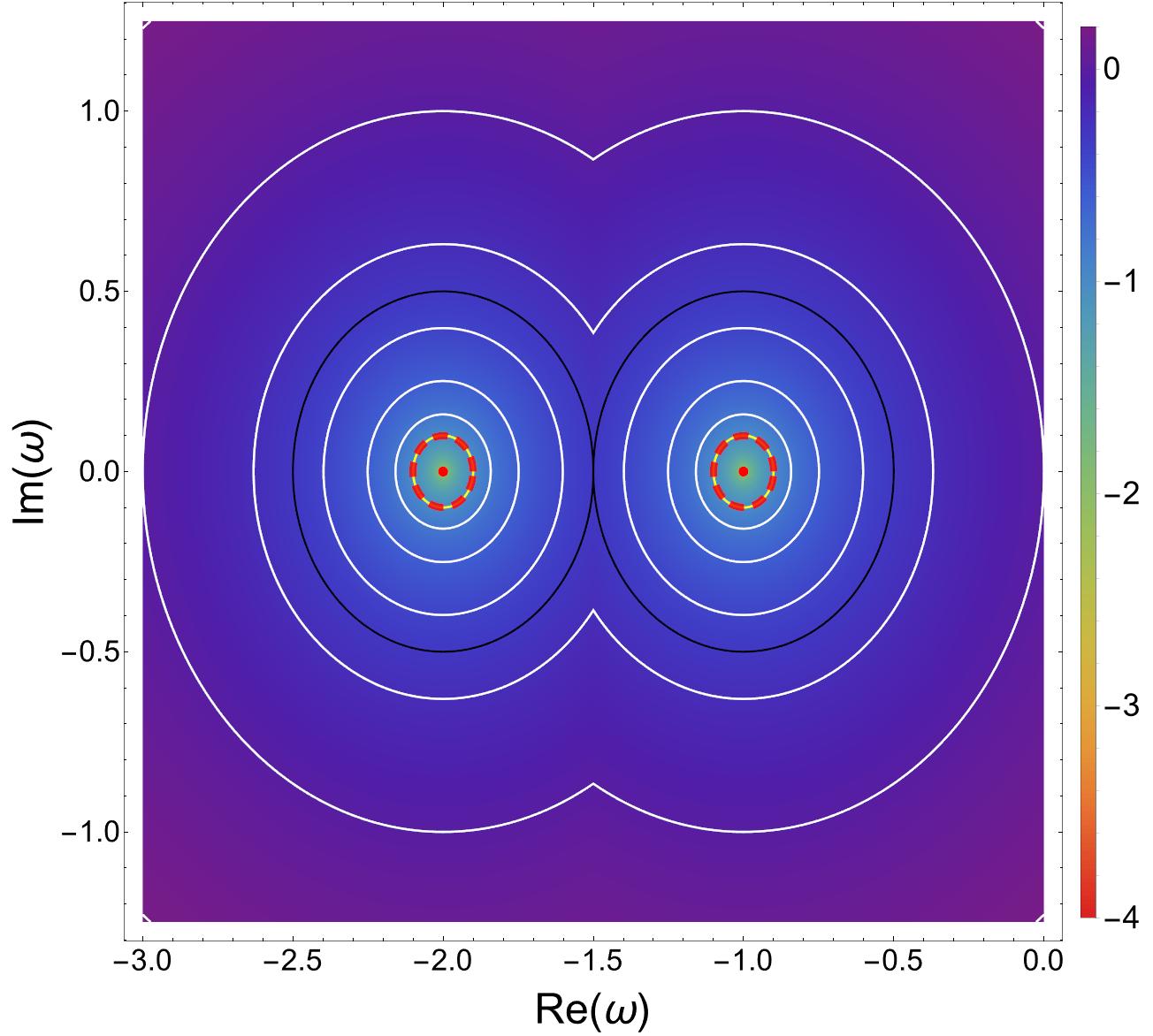
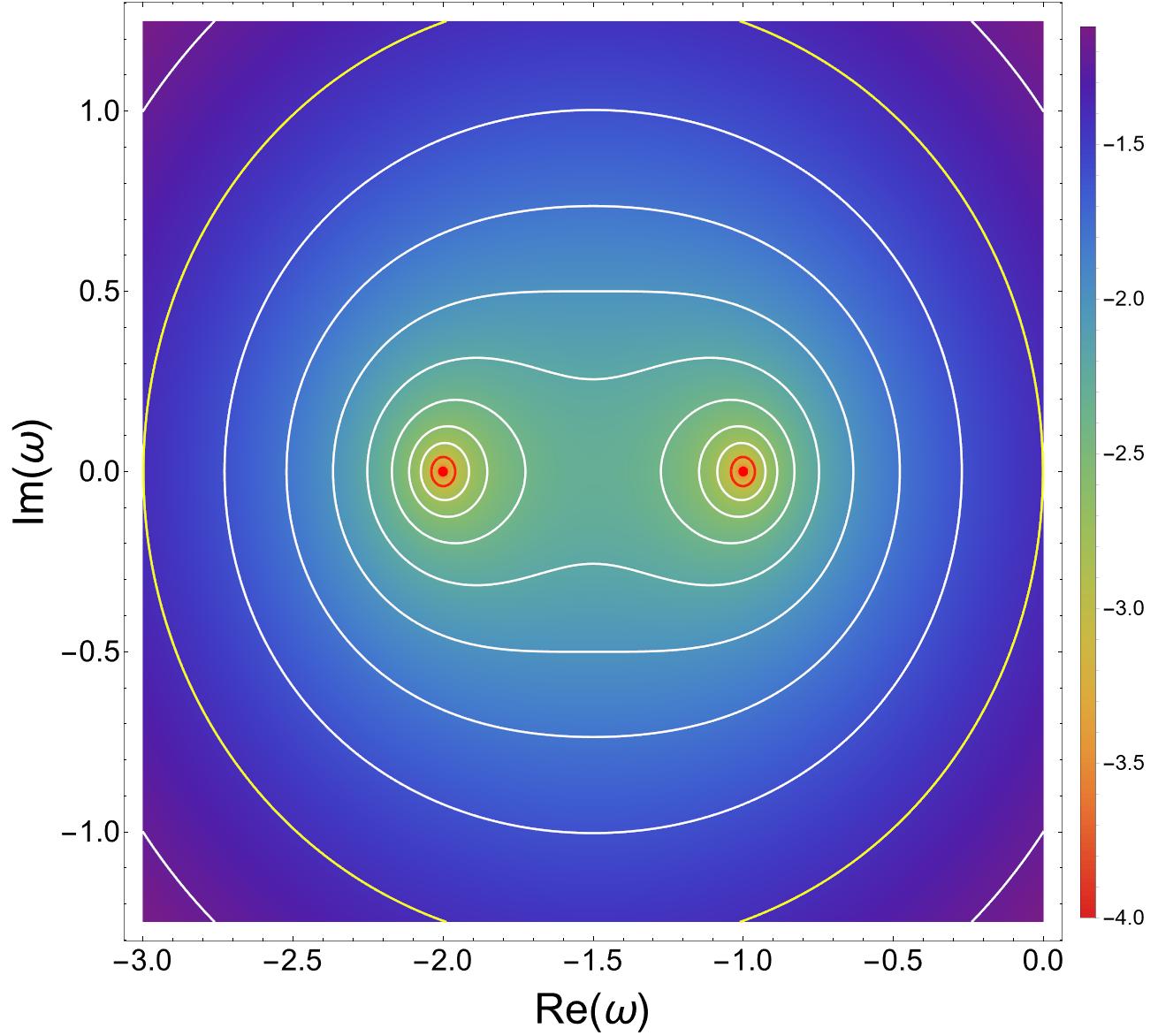
    which differ greatly from 1, and the pseudospectrum of figure 1(a), which is characterized by extended ε𝜀\varepsilon-pseudospectrum boundaries that eventually engulf both eigenvalues for small values of ε𝜀\varepsilon.

  • G𝐺G-norm:

    In this case, A𝐴A is self-adjoint:

    A=G1AG¯=(10502)=A,superscript𝐴¯superscript𝐺1𝐴𝐺matrix10502𝐴A^{\dagger}=\overline{G^{-1}AG}=\begin{pmatrix}-1&0\\ -50&-2\end{pmatrix}=A\,, (47)

    and consequently stable.

    Here, the condition numbers are

    κ1=1,κ2=1,formulae-sequencesubscript𝜅11subscript𝜅21\kappa_{1}=1\,,\qquad\kappa_{2}=1\,, (48)

    and the pseudospectrum is characterized by concentric circles of radius ε𝜀\varepsilon around the eigenvalues (figure 1(b)), both denoting stability.

As expected, the choice of norm is nontrivial; the notion of stability depends on the definition of small perturbations. It is also interesting to remark that figures 1(a) and 1(b) show very common features of the pseudospectrum of non-normal and normal operators, respectively. In general, the ε𝜀\varepsilon-pseudospectrum of a normal operator is a set disks of radius ε𝜀\varepsilon centered on the eigenvalues (as indicated by corollary 2.1); while for a non-normal operator it presents extended regions that may contain multiple eigenvalues.888Note that for normal operators the ε𝜀\varepsilon-pseudospectrum does engulf multiple eigenvalues if ε𝜀\varepsilon is large. As expected, this behaviour appears for ε𝜀\varepsilon larger than half the distance between the two eigenvalues.
Refer to caption
(a) 22subscriptsuperscript22\ell^{2}_{2}-norm
Refer to caption
(b) G𝐺G-norm
Figure 1: Pseudospectrum of the A𝐴A matrix (41) in two different norms. In both figures the red dots correspond to the eigenvalues, the white lines to boundaries of different ε𝜀\varepsilon-pseudospectra and the heat map to the logarithm of the inverse of the resolvent. In (a) the solid red and yellow lines represent the boundaries of σ(A)+Δ0.04𝜎𝐴subscriptΔ0.04\sigma(A)+\Delta_{0.04} and σ0.04(A)subscript𝜎0.04𝐴\sigma_{0.04}(A), respectively; note the great discrepancy associated with the non-normality. On the other hand, in (b) the dashed red line and the solid yellow line are superimposed and correspond to the boundaries of σ(A)+Δ0.1𝜎𝐴subscriptΔ0.1\sigma(A)+\Delta_{0.1} and σ0.1(A)subscript𝜎0.1𝐴\sigma_{0.1}(A), respectively. The solid black line in (b) represents the boundary of σ0.5(A)subscript𝜎0.5𝐴\sigma_{0.5}(A).

3 Quasinormal Modes and Pseudospectra

Quasinormal modes (QNMs) in AdS are solutions to the linearized equations of motion in a black hole background with well-defined quasinormal frequencies (QNFs), subject to outgoing boundary conditions on the horizon and normalizable boundary conditions on the AdS boundary Berti:2009kk .999Imposing normalizable boundary conditions corresponds to choosing source-less excitations in the dual QFT or, equivalently, to selecting solutions where the leading term on the AdS boundary vanishes. Note that in some cases the subleading mode can also be identified with the source; this corresponds to a different choice of quantization scheme in the dual QFT Klebanov:1999tb . For simplicity, in the present work we do not consider that possibility. QNMs are small excitations of the black hole spacetime that eventually fall into the horizon and die out, provided the spacetime is stable.101010Here, stability of the spacetime entails that the perturbation decays as opposed to growing exponentially. From the dual QFT perspective, they correspond to excitations over the thermal equilibrium that eventually thermalize. The decaying behaviour is reflected in the associated QNFs, which are complex as the system is inherently non-conservative.

As argued in the previous section, the spectra of non-conservative systems are potentially unstable. One thus needs to complement the study of QNFs with pseudospectrum analysis. In order to achieve this, we need to cast the problem of finding QNFs as an eigenvalue equation and define a physically motivated norm. In this section we implement these two steps to determine the pseudospectrum of fluctuations in asymptotic AdS black hole geometries.

Specifically, as a background we consider a static (d+1)d1(\text{d}+1)-dimensional AdS planar black hole (black brane) spacetime, whose dual is a d-dimensional strongly coupled QFT in thermal equilibrium at temperature given by the Hawking temperature of the black brane. The corresponding metric in Poincaré coordinates is given by:

ds2=r2l2(f(r)dt2+δijdxidxj)+l2r2dr2f(r),𝑑superscript𝑠2superscript𝑟2superscript𝑙2𝑓𝑟𝑑superscript𝑡2subscript𝛿𝑖𝑗𝑑superscript𝑥𝑖𝑑superscript𝑥𝑗superscript𝑙2superscript𝑟2𝑑superscript𝑟2𝑓𝑟ds^{2}=\frac{r^{2}}{l^{2}}\left(-f(r)dt^{2}+\delta_{ij}dx^{i}dx^{j}\right)+\frac{l^{2}}{r^{2}}\frac{dr^{2}}{f(r)}\,, (49)

where l𝑙l is the AdS radius and f(r)𝑓𝑟f(r) is the blackening factor whose largest zero we denote by rhsubscript𝑟r_{h}. In these coordinates, the Hawking temperature T𝑇T is given by:

T=rh24πl2df(r)dr|r=rh,𝑇evaluated-atsuperscriptsubscript𝑟24𝜋superscript𝑙2𝑑𝑓𝑟𝑑𝑟𝑟subscript𝑟T=\frac{r_{h}^{2}}{4\pi l^{2}}\left.\frac{df(r)}{dr}\right|_{r=r_{h}}\,, (50)

and the AdS boundary and the horizon are located at r=𝑟r=\infty and r=rh𝑟subscript𝑟r=r_{h}, respectively.

3.1 Construction of the Eigenvalue Problem

Our approach relies on utilizing regular coordinates, as introduced in Warnick:2013hba , to express the linearized equations of motion as an eigenvalue problem while also implementing the outgoing boundary conditions as regularity conditions on the horizon.111111Regular coordinates are the AdS equivalent to the hyperboloidal ones used in asymptotically flat spacetimes (see Bizon:2020qnd and PanossoMacedo:2023qzp for a recent overview.).

For the sake of completeness, in this subsection we present the approach in a general setting, only assuming a black brane background.121212Throughout this subsection we will not address the normalizable boundary conditions. As we will see later, these can be easily implemented as Dirichlet or Neumann boundary conditions with an adequate rescaling of the QNMs. In 3.1.1, we specialize this discussion to a scalar in an AdS4+1 Schwarzschild black brane (SAdS4+1) background, hoping to shed more light on the nature of the approach.

In general, we consider linearized equations of motion of the form:

[MM+KMM+U]Φ=0,delimited-[]subscript𝑀superscript𝑀superscript𝐾𝑀subscript𝑀𝑈Φ0\left[-\nabla_{M}\nabla^{M}+K^{M}\nabla_{M}+U\right]\Phi=0\,, (51)

with ΦΦ\Phi a multi-component field, KMsuperscript𝐾𝑀K^{M} and U𝑈U functions and Msubscript𝑀\nabla_{M} the covariant derivative.

Exploiting the symmetries of the black brane, we choose coordinates {𝓉,𝔁,𝓇}𝓉𝔁𝓇\{\mathscr{t},\boldsymbol{\mathscr{x}},\mathscr{r}\} such that the linear operator of equation (51) only depends on 𝓇𝓇\mathscr{r}. Furthermore, in order to eliminate 𝔁𝔁\boldsymbol{\mathscr{x}} derivatives we express ΦΦ\Phi as a superposition of Fourier modes:

Φ(𝓉,𝔁,𝓇)=dd1k(2π)d1Φ(𝓉,𝐤,𝓇)ei𝐤𝔁,Φ𝓉𝔁𝓇superscript𝑑d1𝑘superscript2𝜋d1Φ𝓉𝐤𝓇superscript𝑒𝑖𝐤𝔁\Phi(\mathscr{t},\boldsymbol{\mathscr{x}},\mathscr{r})=\int\frac{d^{\text{d}-1}k}{(2\pi)^{\text{d}-1}}\Phi(\mathscr{t},\mathbf{k},\mathscr{r})e^{i\mathbf{k}\boldsymbol{\mathscr{x}}}\,, (52)

and solve for Φ(𝓉,𝐤,𝓇)Φ𝓉𝐤𝓇\Phi(\mathscr{t},\mathbf{k},\mathscr{r}) instead. We can then rewrite equation (51) as

g𝓉𝓉𝓉2Φ(𝓉,𝐤,𝓇)=F1[𝓇2,𝓇;𝐤,r]Φ(𝓉,𝐤,𝓇)+F2[𝓇;𝐤,r]𝓉Φ(𝓉,𝐤,𝓇),superscript𝑔𝓉𝓉superscriptsubscript𝓉2Φ𝓉𝐤𝓇subscript𝐹1superscriptsubscript𝓇2subscript𝓇𝐤𝑟Φ𝓉𝐤𝓇subscript𝐹2subscript𝓇𝐤𝑟subscript𝓉Φ𝓉𝐤𝓇g^{\mathscr{t}\mathscr{t}}\partial_{\mathscr{t}}^{2}\Phi(\mathscr{t},\mathbf{k},\mathscr{r})=F_{1}\left[\partial_{\mathscr{r}}^{2},\partial_{\mathscr{r}};\mathbf{k},r\right]\Phi(\mathscr{t},\mathbf{k},\mathscr{r})+F_{2}\left[\partial_{\mathscr{r}};\mathbf{k},r\right]\partial_{\mathscr{t}}\Phi(\mathscr{t},\mathbf{k},\mathscr{r})\,, (53)

where F1[𝓇2,𝓇;𝐤,r]subscript𝐹1superscriptsubscript𝓇2subscript𝓇𝐤𝑟F_{1}\left[\partial_{\mathscr{r}}^{2},\partial_{\mathscr{r}};\mathbf{k},r\right] and F2[𝓇;𝐤,r]subscript𝐹2subscript𝓇𝐤𝑟F_{2}\left[\partial_{\mathscr{r}};\mathbf{k},r\right] are differential operators on 𝓇𝓇\mathscr{r} of second and first order, respectively. Then, as long as the 𝓉𝓉\mathscr{t}-hypersurfaces are not null (g𝓉𝓉0superscript𝑔𝓉𝓉0g^{\mathscr{t}\mathscr{t}}\neq 0), we can introduce the auxiliary variable Ψ=𝓉ΦΨsubscript𝓉Φ\Psi=\partial_{\mathscr{t}}\Phi and rewrite the equations of motion (53) as:131313For notational convenience, we refer to the xM=constsuperscript𝑥𝑀constx^{M}=\text{const} hypersurface as xMsuperscript𝑥𝑀x^{M}-hypersurface.

𝓉(Φ(𝓉,𝐤,𝓇)Ψ(𝓉,𝐤,𝓇))=(01L1[𝓇2,𝓇;𝐤,r]L2[𝓇;𝐤,r])(Φ(𝓉,𝐤,𝓇)Ψ(𝓉,𝐤,𝓇)),subscript𝓉matrixΦ𝓉𝐤𝓇Ψ𝓉𝐤𝓇matrix01subscript𝐿1superscriptsubscript𝓇2subscript𝓇𝐤𝑟subscript𝐿2subscript𝓇𝐤𝑟matrixΦ𝓉𝐤𝓇Ψ𝓉𝐤𝓇\partial_{\mathscr{t}}\begin{pmatrix}\Phi(\mathscr{t},\mathbf{k},\mathscr{r})\\ \Psi(\mathscr{t},\mathbf{k},\mathscr{r})\end{pmatrix}=\begin{pmatrix}0&1\\ L_{1}\left[\partial_{\mathscr{r}}^{2},\partial_{\mathscr{r}};\mathbf{k},r\right]&L_{2}\left[\partial_{\mathscr{r}};\mathbf{k},r\right]\end{pmatrix}\begin{pmatrix}\Phi(\mathscr{t},\mathbf{k},\mathscr{r})\\ \Psi(\mathscr{t},\mathbf{k},\mathscr{r})\end{pmatrix}\,, (54)

where we have defined Li=(g𝓉𝓉)1Fisubscript𝐿𝑖superscriptsuperscript𝑔𝓉𝓉1subscript𝐹𝑖L_{i}=\left(g^{\mathscr{t}\mathscr{t}}\right)^{-1}F_{i}.

Recalling that a QNM Φ(𝓉,𝐤,𝓇)Φ𝓉𝐤𝓇\Phi(\mathscr{t},\mathbf{k},\mathscr{r}) has a well-defined QNF ω𝜔\omega or, equivalently, that it is an eigenfunction of the Killing vector associated with stationarity, 𝔱=𝓉𝔱subscript𝓉\mathfrak{t}=\partial_{\mathscr{t}}:

𝔱(Φ(𝓉,𝐤,𝓇)Ψ(𝓉,𝐤,𝓇))=𝓉(Φ(𝓉,𝐤,𝓇)Ψ(𝓉,𝐤,𝓇))=iω(Φ(𝓉,𝐤,𝓇)Ψ(𝓉,𝐤,𝓇)),𝔱matrixΦ𝓉𝐤𝓇Ψ𝓉𝐤𝓇subscript𝓉matrixΦ𝓉𝐤𝓇Ψ𝓉𝐤𝓇𝑖𝜔matrixΦ𝓉𝐤𝓇Ψ𝓉𝐤𝓇\mathfrak{t}\begin{pmatrix}\Phi(\mathscr{t},\mathbf{k},\mathscr{r})\\ \Psi(\mathscr{t},\mathbf{k},\mathscr{r})\end{pmatrix}=\partial_{\mathscr{t}}\begin{pmatrix}\Phi(\mathscr{t},\mathbf{k},\mathscr{r})\\ \Psi(\mathscr{t},\mathbf{k},\mathscr{r})\end{pmatrix}=-i\omega\begin{pmatrix}\Phi(\mathscr{t},\mathbf{k},\mathscr{r})\\ \Psi(\mathscr{t},\mathbf{k},\mathscr{r})\end{pmatrix}\,, (55)

we can cast expression (54) as a standard eigenvalue problem:

ω(Φ(𝓉,𝐤,𝓇)Ψ(𝓉,𝐤,𝓇))=i(01L1[𝓇2,𝓇;𝐤,r]L2[𝓇;𝐤,r])(Φ(𝓉,𝐤,𝓇)Ψ(𝓉,𝐤,𝓇)).𝜔matrixΦ𝓉𝐤𝓇Ψ𝓉𝐤𝓇𝑖matrix01subscript𝐿1superscriptsubscript𝓇2subscript𝓇𝐤𝑟subscript𝐿2subscript𝓇𝐤𝑟matrixΦ𝓉𝐤𝓇Ψ𝓉𝐤𝓇\omega\begin{pmatrix}\Phi(\mathscr{t},\mathbf{k},\mathscr{r})\\ \Psi(\mathscr{t},\mathbf{k},\mathscr{r})\end{pmatrix}=i\begin{pmatrix}0&1\\ L_{1}\left[\partial_{\mathscr{r}}^{2},\partial_{\mathscr{r}};\mathbf{k},r\right]&L_{2}\left[\partial_{\mathscr{r}};\mathbf{k},r\right]\end{pmatrix}\begin{pmatrix}\Phi(\mathscr{t},\mathbf{k},\mathscr{r})\\ \Psi(\mathscr{t},\mathbf{k},\mathscr{r})\end{pmatrix}\,. (56)

Note that to write the equations of motion as an eigenvalue problem it is fundamental that the 𝓉𝓉\mathscr{t}-hypersurfaces are spacelike as opposed to null. Otherwise, we would obtain a generalized eigenvalue equation of the form:

ωF2[𝓇;𝐤,r]Φ(𝓉,𝐤,𝓇)=iF1[𝓇2,𝓇;𝐤,r]Φ(𝓉,𝐤,𝓇),𝜔subscript𝐹2subscript𝓇𝐤𝑟Φ𝓉𝐤𝓇𝑖subscript𝐹1superscriptsubscript𝓇2subscript𝓇𝐤𝑟Φ𝓉𝐤𝓇\omega F_{2}\left[\partial_{\mathscr{r}};\mathbf{k},r\right]\Phi(\mathscr{t},\mathbf{k},\mathscr{r})=-iF_{1}\left[\partial_{\mathscr{r}}^{2},\partial_{\mathscr{r}};\mathbf{k},r\right]\Phi(\mathscr{t},\mathbf{k},\mathscr{r})\,, (57)

instead of the standard eigenvalue problem discussed in section 2.141414Technically, one can extend the formalism presented in section 2 to also hold for generalized eigenvalue problems of the form (LλA)u=0𝐿𝜆𝐴𝑢0\left(L-\lambda A\right)u=0. However, the adequate notion of ε𝜀\varepsilon-pseudospectrum becomes unclear as one has to choose whether to perturb L𝐿L, A𝐴A or both (see Chapter 45 of Trefethen:2005 and references therein for an extensive discussion).

Regarding the boundary conditions, we seek to choose {𝓉,𝔁,𝓇}𝓉𝔁𝓇\{\mathscr{t},\boldsymbol{\mathscr{x}},\mathscr{r}\} such that demanding regularity on the horizon is equivalent to imposing outgoing boundary conditions. This is typically achieved working with infalling Eddington Finkenstein (IEF) coordinates {u,𝐱~,r~}𝑢~𝐱~𝑟\{u,\tilde{\mathbf{x}},\tilde{r}\}, which, in terms of the Poincaré coordinates {t,𝐱,r}𝑡𝐱𝑟\{t,\mathbf{x},r\}, are given by:

u=t+drf(r)(lr)2,𝐱~=𝐱,r~=r.formulae-sequence𝑢𝑡𝑑𝑟𝑓𝑟superscript𝑙𝑟2formulae-sequence~𝐱𝐱~𝑟𝑟u=t+\int\frac{dr}{f(r)}\left(\frac{l}{r}\right)^{2}\,,\qquad\tilde{\mathbf{x}}=\mathbf{x}\,,\qquad\tilde{r}=r\,. (58)

However, writing the metric (49) in IEF coordinates:

ds2=r~2l2(f(r~)du2+δijdxidxj)+2dudr~,𝑑superscript𝑠2superscript~𝑟2superscript𝑙2𝑓~𝑟𝑑superscript𝑢2subscript𝛿𝑖𝑗𝑑superscript𝑥𝑖𝑑superscript𝑥𝑗2𝑑𝑢𝑑~𝑟ds^{2}=\frac{\tilde{r}^{2}}{l^{2}}\left(-f(\tilde{r})du^{2}+\delta_{ij}dx^{i}dx^{j}\right)+2dud\tilde{r}\,, (59)

we conclude that the u𝑢u-hypersurfaces are null and thus IEF coordinates are ill-suited for pseudospectrum analysis.

Nonetheless, we can define regular coordinates that resemble the IEF ones near the horizon having spacelike 𝓉𝓉\mathscr{t}-hypersurfaces outside the horizon. More concretely, we construct regular coordinates such that the spacelike 𝓉𝓉\mathscr{t}-hypersurfaces match the null IEF u𝑢u-hypersurfaces exactly on the horizon. A particularly simple choice is given by:

𝓉=ul2rh(1rhr~)=tl2rh(1rhr)+drf(r)(lr)2,𝔁=𝐱~=𝐱,𝓇=r~=r,formulae-sequence𝓉𝑢superscript𝑙2subscript𝑟1subscript𝑟~𝑟𝑡superscript𝑙2subscript𝑟1subscript𝑟𝑟𝑑𝑟𝑓𝑟superscript𝑙𝑟2𝔁~𝐱𝐱𝓇~𝑟𝑟\mathscr{t}=u-\frac{l^{2}}{r_{h}}\left(1-\frac{r_{h}}{\tilde{r}}\right)=t-\frac{l^{2}}{r_{h}}\left(1-\frac{r_{h}}{r}\right)+\int\frac{dr}{f(r)}\left(\frac{l}{r}\right)^{2}\,,\qquad\boldsymbol{\mathscr{x}}=\tilde{\mathbf{x}}=\mathbf{x}\,,\qquad\mathscr{r}=\tilde{r}=r\,, (60)

in terms of which the metric (49) is:

ds2=𝓇2l2(f(𝓇)d𝓉2+δijd𝓍id𝓍j)+2(1f(𝓇))d𝓉d𝓇+l2𝓇2(2f(𝓇))d𝓇2.𝑑superscript𝑠2superscript𝓇2superscript𝑙2𝑓𝓇𝑑superscript𝓉2subscript𝛿𝑖𝑗𝑑superscript𝓍𝑖𝑑superscript𝓍𝑗21𝑓𝓇𝑑𝓉𝑑𝓇superscript𝑙2superscript𝓇22𝑓𝓇𝑑superscript𝓇2ds^{2}=\frac{\mathscr{r}^{2}}{l^{2}}\left(-f(\mathscr{r})d\mathscr{t}^{2}+\delta_{ij}d\mathscr{x}^{i}d\mathscr{x}^{j}\right)+2\left(1-f(\mathscr{r})\right)d\mathscr{t}d\mathscr{r}+\frac{l^{2}}{\mathscr{r}^{2}}\left(2-f(\mathscr{r})\right)d\mathscr{r}^{2}\,. (61)

In practice, for most numerical applications it is more convenient to introduce a dimensionless compactified radial coordinate ρ𝜌\rho:

ρ=1rh𝓇,𝜌1subscript𝑟𝓇\rho=1-\frac{r_{h}}{\mathscr{r}}\,, (62)

such that the horizon is mapped to ρ=0𝜌0\rho=0 and the AdS boundary to ρ=1𝜌1\rho=1. In terms of these compactified regular coordinates {𝓉,𝔁,ρ}𝓉𝔁𝜌\{\mathscr{t},\boldsymbol{\mathscr{x}},\rho\}, the black brane metric (49) takes the form:

ds2=l2zh2(1ρ)2(𝒻(ρ)d𝓉2+δijd𝓍id𝓍j+2(1𝒻(ρ))zhd𝓉dρ+(2𝒻(ρ))zh2dρ2).𝑑superscript𝑠2superscript𝑙2superscriptsubscript𝑧2superscript1𝜌2𝒻𝜌𝑑superscript𝓉2subscript𝛿𝑖𝑗𝑑superscript𝓍𝑖𝑑superscript𝓍𝑗21𝒻𝜌subscript𝑧𝑑𝓉𝑑𝜌2𝒻𝜌superscriptsubscript𝑧2𝑑superscript𝜌2ds^{2}=\frac{l^{2}}{z_{h}^{2}(1-\rho)^{2}}\left(-\mathscr{f}(\rho)d\mathscr{t}^{2}+\delta_{ij}d\mathscr{x}^{i}d\mathscr{x}^{j}+2\left(1-\mathscr{f}(\rho)\right)z_{h}d\mathscr{t}d\rho+\left(2-\mathscr{f}(\rho)\right)z_{h}^{2}d\rho^{2}\right)\,. (63)

where 𝒻(ρ)=f(r(ρ))𝒻𝜌𝑓𝑟𝜌\mathscr{f}(\rho)=f\left(r\left(\rho\right)\right) and zh=l2/rhsubscript𝑧superscript𝑙2subscript𝑟z_{h}=l^{2}/r_{h}.

It is worth stressing that the components of the Killing vector 𝔱=𝓉=t𝔱subscript𝓉subscript𝑡\mathfrak{t}=\partial_{\mathscr{t}}=\partial_{t} are invariant under the change of coordinates from regular to Poincaré coordinates. Consequently, the QNFs defined as the eigenvalues of tsubscript𝑡\partial_{t} and 𝓉subscript𝓉\partial_{\mathscr{t}} match. In gauge/gravity duality, this is actually important, as the holographic dictionary identifies the poles of the retarded propagators with the eigenvalues of tsubscript𝑡\partial_{t}.151515Here, by the holographic dictionary we refer to the standard one formulated in Poincaré coordinates. Note that one can always formulate a new holographic dictionary in a different coordinate set and identify the QNFs with the poles of the retarded propagators.

Before moving on to a concrete example we summarize the core principles behind the regular coordinates: Given an AdSd+1d1{}_{\text{d}+1} black brane spacetime whose metric in Poincaré coordinates is given by equation (49) a regular coordinate set {𝓉,𝔁,𝓇}𝓉𝔁𝓇\{\mathscr{t},\boldsymbol{\mathscr{x}},\mathscr{r}\} is one that fulfils the following three requirements: the metric components are functions only of 𝓇𝓇\mathscr{r}, 𝓉𝓉\mathscr{t}-hypersurfaces are spacelike outside the horizon, and those 𝓉𝓉\mathscr{t}-hypersurfaces match the IEF u𝑢u-hypersurfaces on the horizon. With these coordinates imposing outgoing boundary conditions corresponds to demanding regularity on the horizon. Moreover, equations of motion for the QNMs of the form (51) can be written as a standard eigenvalue problem.

3.1.1 Example: Real Scalar in SAdS4+1subscriptSAdS41\text{SAdS}_{4+1}

To better clarify the role played by the regular coordinates in the construction of the eigenvalue problem, here we specialize the discussion to a real scalar field ϕitalic-ϕ\phi with action

𝒮[ϕ]=12d4+1xg(MϕMϕ+m2ϕ2),𝒮delimited-[]italic-ϕ12superscript𝑑41𝑥𝑔subscript𝑀italic-ϕsuperscript𝑀italic-ϕsuperscript𝑚2superscriptitalic-ϕ2\mathcal{S}[\phi]=-\frac{1}{2}\int d^{4+1}x\sqrt{-g}\,\,\left(\partial_{M}\phi\partial^{M}\phi+m^{2}\phi^{2}\right)\,, (64)

in a SAdS4+1 background. The corresponding linearized equations of motion are given by:

[MM+m2]ϕ=0.delimited-[]subscript𝑀superscript𝑀superscript𝑚2italic-ϕ0\left[-\nabla_{M}\nabla^{M}+m^{2}\right]\phi=0\,. (65)

For better emphasis on the key aspects of our approach, we present this discussion in Poincaré, IEF and compactified regular coordinates.

Poincaré Coordinates: the SAdS4+1 metric in Poincaré coordinates is given by (49) with f(r)=1(rhr)4𝑓𝑟1superscriptsubscript𝑟𝑟4f(r)=1-\left(\frac{r_{h}}{r}\right)^{4} and {i,j}=1,2,3𝑖𝑗123\{i,j\}=1,2,3. In terms of the Fourier modes ϕ(t,𝐤,r)italic-ϕ𝑡𝐤𝑟\phi(t,\mathbf{k},r), the linearized equation of motion (65) for a QNM trivially produces the following eigenvalue problem:

ω2ϕ(t,𝐤,r)=f(r)[𝐤2+m2r2l2(r5f(r))rl4rr4f(r)l4r2]ϕ(t,𝐤,r),superscript𝜔2italic-ϕ𝑡𝐤𝑟𝑓𝑟delimited-[]superscript𝐤2superscript𝑚2superscript𝑟2superscript𝑙2superscriptsuperscript𝑟5𝑓𝑟𝑟superscript𝑙4subscript𝑟superscript𝑟4𝑓𝑟superscript𝑙4superscriptsubscript𝑟2italic-ϕ𝑡𝐤𝑟\omega^{2}\,\phi(t,\mathbf{k},r)=f(r)\left[\mathbf{k}^{2}+\frac{m^{2}r^{2}}{l^{2}}-\frac{\left(r^{5}f(r)\right)^{\prime}}{rl^{4}}\partial_{r}-\frac{r^{4}f(r)}{l^{4}}\partial_{r}^{2}\right]\phi(t,\mathbf{k},r)\,, (66)

where we have used that the QNM is an eigenfunction of tsubscript𝑡\partial_{t} with QNF ω𝜔\omega.

In order to impose outgoing boundary conditions, we first analyze the behaviour near the horizon r=rh𝑟subscript𝑟r=r_{h}. Solving the equations of motion with a Frobenius series, we find:

ϕ(t,𝐤,r)=eiωt{c1exp[iωl24rhlog(rrh)](1+)+c2exp[iωl24rhlog(rrh)](1+)}.italic-ϕ𝑡𝐤𝑟superscript𝑒𝑖𝜔𝑡subscript𝑐1𝑖𝜔superscript𝑙24subscript𝑟𝑟subscript𝑟1subscript𝑐2𝑖𝜔superscript𝑙24subscript𝑟𝑟subscript𝑟1\phi(t,\mathbf{k},r)=e^{-i\omega t}\left\{c_{1}\exp\left[-i\frac{\omega l^{2}}{4r_{h}}\log(r-r_{h})\right]\left(1+...\right)+c_{2}\exp\left[i\frac{\omega l^{2}}{4r_{h}}\log(r-r_{h})\right]\left(1+...\right)\right\}\,. (67)

Then, as the outgoing solution corresponds to fixing c2=0subscript𝑐20c_{2}=0, imposing outgoing boundary conditions correspond to fixing a near-horizon behaviour:

ϕ(t,𝐤,rrh)c1exp[iω(t+l24rhlog(rrh))].italic-ϕ𝑡𝐤𝑟subscript𝑟subscript𝑐1𝑖𝜔𝑡superscript𝑙24subscript𝑟𝑟subscript𝑟\phi(t,\mathbf{k},r\rightarrow r_{h})\approx c_{1}\exp\left[-i\omega\left(t+\frac{l^{2}}{4r_{h}}\log(r-r_{h})\right)\right]\,. (68)

Note that this choice for the outgoing solution matches our physical interpretation of a mode that falls into the horizon. Defining the tortoise coordinate rsubscript𝑟r_{*}

r=l22rh[arctan(rrh)arctanh(rhr)]=l24rhlog(rrh)+𝒪((rrh)0),subscript𝑟superscript𝑙22subscript𝑟delimited-[]arctangent𝑟subscript𝑟arctanhsubscript𝑟𝑟superscript𝑙24subscript𝑟𝑟subscript𝑟𝒪superscript𝑟subscript𝑟0r_{*}=\frac{l^{2}}{2r_{h}}\left[\arctan\left(\frac{r}{r_{h}}\right)-\operatorname{arctanh}\left(\frac{r_{h}}{r}\right)\right]=\frac{l^{2}}{4r_{h}}\log(r-r_{h})+\mathcal{O}\left((r-r_{h})^{0}\right)\,, (69)

the near-horizon behaviour can be written as two modes, one falling towards the brane and one exiting it:

ϕ(t,𝐤,rrh)c1exp[iω(t+r)]+c2exp[iω(tr)],italic-ϕ𝑡𝐤𝑟subscript𝑟subscript𝑐1𝑖𝜔𝑡subscript𝑟subscript𝑐2𝑖𝜔𝑡subscript𝑟\phi(t,\mathbf{k},r\rightarrow r_{h})\approx c_{1}\exp\left[-i\omega\left(t+r_{*}\right)\right]+c_{2}\exp\left[-i\omega\left(t-r_{*}\right)\right]\,, (70)

and choosing a QNM that falls into the horizon corresponds to discarding the ingoing mode, i.e., taking c2=0subscript𝑐20c_{2}=0.

IEF Coordinates: the SAdS4+1 metric in IEF coordinates is given by (59) with f(r~)=1(rhr~)4𝑓~𝑟1superscriptsubscript𝑟~𝑟4f(\tilde{r})=1-\left(\frac{r_{h}}{\tilde{r}}\right)^{4} and {i,j}=1,2,3𝑖𝑗123\{i,j\}=1,2,3. The linearized equation of motion for a QNM (65) reads:

ω[3r~+2r~]ϕ(u,𝐤,r~)=i[𝐤2l2r~2+m2(r~5f(r~))r~3l2r~r~2f(r~)l2r~2]ϕ(u,𝐤,r~),𝜔delimited-[]3~𝑟2subscript~𝑟italic-ϕ𝑢𝐤~𝑟𝑖delimited-[]superscript𝐤2superscript𝑙2superscript~𝑟2superscript𝑚2superscriptsuperscript~𝑟5𝑓~𝑟superscript~𝑟3superscript𝑙2subscript~𝑟superscript~𝑟2𝑓~𝑟superscript𝑙2superscriptsubscript~𝑟2italic-ϕ𝑢𝐤~𝑟\omega\left[\frac{3}{\tilde{r}}+2\partial_{\tilde{r}}\right]\phi(u,\mathbf{k},\tilde{r})=i\left[\frac{\mathbf{k}^{2}l^{2}}{\tilde{r}^{2}}+m^{2}-\frac{\left(\tilde{r}^{5}f(\tilde{r})\right)^{\prime}}{\tilde{r}^{3}l^{2}}\partial_{\tilde{r}}-\frac{\tilde{r}^{2}f(\tilde{r})}{l^{2}}\partial_{\tilde{r}}^{2}\right]\phi(u,\mathbf{k},\tilde{r})\,, (71)

and it cannot be cast as a standard eigenvalue problem due to the derivative term. The near-horizon solution is given by:

ϕ(u,𝐤,r~)=eiωu{c1(1+)+c2exp[iωl22rhlog(r~rh)](1+)},italic-ϕ𝑢𝐤~𝑟superscript𝑒𝑖𝜔𝑢subscript𝑐11subscript𝑐2𝑖𝜔superscript𝑙22subscript𝑟~𝑟subscript𝑟1\phi(u,\mathbf{k},\tilde{r})=e^{-i\omega u}\left\{c_{1}\left(1+...\right)+c_{2}\exp\left[i\frac{\omega l^{2}}{2r_{h}}\log(\tilde{r}-r_{h})\right]\left(1+...\right)\right\}\,, (72)

with the outgoing solution corresponding to fixing c2=0subscript𝑐20c_{2}=0.161616This follows from the Poincaré result noting that under the coordinate transformation (58) we have: eiωu=exp[iω(t+l24rhlog(rrh))]+𝒪((rrh)0).superscript𝑒𝑖𝜔𝑢𝑖𝜔𝑡superscript𝑙24subscript𝑟𝑟subscript𝑟𝒪superscript𝑟subscript𝑟0e^{-i\omega u}=\exp\left[-i\omega\left(t+\frac{l^{2}}{4r_{h}}\log\left(r-r_{h}\right)\right)\right]+\mathcal{O}\left((r-r_{h})^{0}\right)\,. Consequently, imposing outgoing boundary conditions corresponds to demanding regularity on the horizon:

ϕ(t,𝐤,r~rh)c1eiωu.italic-ϕ𝑡𝐤~𝑟subscript𝑟subscript𝑐1superscript𝑒𝑖𝜔𝑢\phi(t,\mathbf{k},\tilde{r}\rightarrow r_{h})\approx c_{1}e^{-i\omega u}\,. (73)

Compactified Regular Coordinates: the SAdS4+1 metric in compactified regular coordinates {𝓉,𝔁,ρ}𝓉𝔁𝜌\{\mathscr{t},\boldsymbol{\mathscr{x}},\rho\} is given by (63) with 𝒻(ρ)=1(1ρ)4𝒻𝜌1superscript1𝜌4\mathscr{f}(\rho)=1-\left(1-\rho\right)^{4} and {i,j}=1,2,3𝑖𝑗123\{i,j\}=1,2,3. Then, the linearized equation of motion for a QNM (65) is:

zh2ω2[𝒻(ρ)2]ϕ(𝓉,𝐤,𝓇)=izhω[(1ρ)3(𝒻(ρ)1(1ρ)3)+2(𝒻(ρ)1)ρ]ϕ(𝓉,𝐤,𝓇)superscriptsubscript𝑧2superscript𝜔2delimited-[]𝒻𝜌2italic-ϕ𝓉𝐤𝓇𝑖subscript𝑧𝜔delimited-[]superscript1𝜌3superscript𝒻𝜌1superscript1𝜌32𝒻𝜌1subscript𝜌italic-ϕ𝓉𝐤𝓇\displaystyle z_{h}^{2}\omega^{2}\left[\mathscr{f}(\rho)-2\right]\phi(\mathscr{t},\mathbf{k},\mathscr{r})=iz_{h}\omega\left[(1-\rho)^{3}\left(\frac{\mathscr{f}(\rho)-1}{(1-\rho)^{3}}\right)^{\prime}+2\left(\mathscr{f}(\rho)-1\right)\partial_{\rho}\right]\phi(\mathscr{t},\mathbf{k},\mathscr{r})
[m2l2(1ρ)2+zh2𝐤2(1ρ)3(𝒻(ρ)(1ρ)3)ρ𝒻(ρ)ρ2]ϕ(𝓉,𝐤,𝓇),delimited-[]superscript𝑚2superscript𝑙2superscript1𝜌2superscriptsubscript𝑧2superscript𝐤2superscript1𝜌3superscript𝒻𝜌superscript1𝜌3subscript𝜌𝒻𝜌superscriptsubscript𝜌2italic-ϕ𝓉𝐤𝓇\displaystyle-\left[\frac{m^{2}l^{2}}{(1-\rho)^{2}}+z_{h}^{2}\mathbf{k}^{2}-(1-\rho)^{3}\left(\frac{\mathscr{f}(\rho)}{(1-\rho)^{3}}\right)^{\prime}\partial_{\rho}-\mathscr{f}(\rho)\partial_{\rho}^{2}\right]\phi(\mathscr{t},\mathbf{k},\mathscr{r})\,, (74)

and, introducing the dimensionless variables

𝔴=zhω=ωπT,𝖖=zh𝐤=𝐤πT,formulae-sequence𝔴subscript𝑧𝜔𝜔𝜋𝑇𝖖subscript𝑧𝐤𝐤𝜋𝑇\mathfrak{w}=z_{h}\omega=\frac{\omega}{\pi T}\,,\quad\boldsymbol{\mathfrak{q}}=z_{h}\mathbf{k}=\frac{\mathbf{k}}{\pi T}\,, (75)

and the auxiliary field ψ(𝓉,𝐤,𝓇)=zh𝓉ϕ(𝓉,𝐤,𝓇)𝜓𝓉𝐤𝓇subscript𝑧subscript𝓉italic-ϕ𝓉𝐤𝓇\psi(\mathscr{t},\mathbf{k},\mathscr{r})=z_{h}\partial_{\mathscr{t}}\phi(\mathscr{t},\mathbf{k},\mathscr{r}), equation (3.1.1) can be written as an eigenvalue problem 171717One could cast the eigenvalue problem without introducing the dimensionless variables 𝔴𝔴\mathfrak{w} and 𝖖𝖖\boldsymbol{\mathfrak{q}}. However, it is convenient to use them as they allows us to remove all zhsubscript𝑧z_{h} dependence and thus reduce the parameter space.

𝔴(ϕ(𝓉,𝐤,ρ)ψ(𝓉,𝐤,ρ))=i(01L1[ρ2,ρ;𝖖,ρ]L2[ρ;𝖖,ρ])(ϕ(𝓉,𝐤,ρ)ψ(𝓉,𝐤,ρ)),𝔴matrixitalic-ϕ𝓉𝐤𝜌𝜓𝓉𝐤𝜌𝑖matrix01subscript𝐿1superscriptsubscript𝜌2subscript𝜌𝖖𝜌subscript𝐿2subscript𝜌𝖖𝜌matrixitalic-ϕ𝓉𝐤𝜌𝜓𝓉𝐤𝜌\mathfrak{w}\begin{pmatrix}\phi(\mathscr{t},\mathbf{k},\rho)\\ \psi(\mathscr{t},\mathbf{k},\rho)\end{pmatrix}=i\begin{pmatrix}0&1\\ L_{1}\left[\partial_{\mathscr{\rho}}^{2},\partial_{\mathscr{\rho}};\boldsymbol{\mathfrak{q}},\rho\right]&L_{2}\left[\partial_{\rho};\boldsymbol{\mathfrak{q}},\rho\right]\end{pmatrix}\begin{pmatrix}\phi(\mathscr{t},\mathbf{k},\rho)\\ \psi(\mathscr{t},\mathbf{k},\rho)\end{pmatrix}\,, (76)

where the differential operators L1subscript𝐿1L_{1} and L2subscript𝐿2L_{2} take the form:

L1[ρ2,ρ;𝖖,ρ]subscript𝐿1superscriptsubscript𝜌2subscript𝜌𝖖𝜌\displaystyle L_{1}\left[\partial_{\rho}^{2},\partial_{\rho};\boldsymbol{\mathfrak{q}},\rho\right] =[𝒻(ρ)2]1[m2l2(1ρ)2+𝖖2(1ρ)3(𝒻(ρ)(1ρ)3)ρ𝒻(ρ)ρ2],absentsuperscriptdelimited-[]𝒻𝜌21delimited-[]superscript𝑚2superscript𝑙2superscript1𝜌2superscript𝖖2superscript1𝜌3superscript𝒻𝜌superscript1𝜌3subscript𝜌𝒻𝜌superscriptsubscript𝜌2\displaystyle=\left[\mathscr{f}(\rho)-2\right]^{-1}\left[\frac{m^{2}l^{2}}{(1-\rho)^{2}}+\boldsymbol{\mathfrak{q}}^{2}-(1-\rho)^{3}\left(\frac{\mathscr{f}(\rho)}{(1-\rho)^{3}}\right)^{\prime}\partial_{\rho}-\mathscr{f}(\rho)\partial_{\rho}^{2}\right]\,, (77)
L2[ρ;𝖖,ρ]subscript𝐿2subscript𝜌𝖖𝜌\displaystyle L_{2}\left[\partial_{\rho};\boldsymbol{\mathfrak{q}},\rho\right] =[𝒻(ρ)2]1[(1ρ)3(𝒻(ρ)1(1ρ)3)+2(𝒻(ρ)1)ρ].absentsuperscriptdelimited-[]𝒻𝜌21delimited-[]superscript1𝜌3superscript𝒻𝜌1superscript1𝜌32𝒻𝜌1subscript𝜌\displaystyle=\left[\mathscr{f}(\rho)-2\right]^{-1}\left[(1-\rho)^{3}\left(\frac{\mathscr{f}(\rho)-1}{(1-\rho)^{3}}\right)^{\prime}+2\left(\mathscr{f}(\rho)-1\right)\partial_{\rho}\right]\,. (78)

With regard to the near-horizon behaviour, we have:

ϕ(𝓉,𝐤,ρ)=eiω𝓉{c1(1+)+c2ρexp[izhω2log(ρ)](1+)},italic-ϕ𝓉𝐤𝜌superscript𝑒𝑖𝜔𝓉subscript𝑐11subscript𝑐2𝜌𝑖subscript𝑧𝜔2𝜌1\phi(\mathscr{t},\mathbf{k},\rho)=e^{-i\omega\mathscr{t}}\left\{c_{1}\left(1+...\right)+c_{2}\rho\exp\left[i\frac{z_{h}\omega}{2}\log(\rho)\right]\left(1+...\right)\right\}\,, (79)

with the outgoing solution corresponding to fixing c2=0subscript𝑐20c_{2}=0.181818Once again, this follows from the Poincaré result as under the coordinate transformation (60) we have: eiω𝓉=exp[iω(t+l24rhlog(rrh))]+𝒪((rrh)0).superscript𝑒𝑖𝜔𝓉𝑖𝜔𝑡superscript𝑙24subscript𝑟𝑟subscript𝑟𝒪superscript𝑟subscript𝑟0e^{-i\omega\mathscr{t}}=\exp\left[-i\omega\left(t+\frac{l^{2}}{4r_{h}}\log\left(r-r_{h}\right)\right)\right]+\mathcal{O}\left((r-r_{h})^{0}\right)\,. Then, imposing outgoing boundary conditions corresponds to demanding regularity on the horizon:

ϕ(𝓉,𝐤,ρ0)c1eiω𝓉.italic-ϕ𝓉𝐤𝜌0subscript𝑐1superscript𝑒𝑖𝜔𝓉\phi(\mathscr{t},\mathbf{k},\rho\rightarrow 0)\approx c_{1}e^{-i\omega\mathscr{t}}\,. (80)

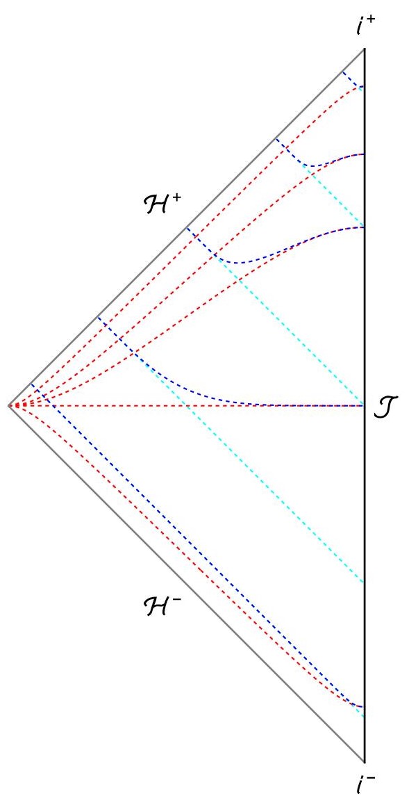
Therefore, it is clear that the regular coordinates constitute a sort of middle ground between IEF and Poincaré coordinates. They exploit the regular behaviour on the horizon of the IEF coordinates while maintaining the spacelike character of the constant time hypersurfaces found in Poincaré coordinates. In fact, with our particular choice of regular coordinates, the 𝓉𝓉\mathscr{t}-hypersurfaces can be thought of as interpolating between u𝑢u- and t𝑡t-hypersurfaces (see figure 2).

Refer to caption
Figure 2: Penrose Diagram of SAdS4+1. The AdS boundary is denoted by 𝒥𝒥\mathcal{J}, +superscript\mathcal{H}^{+} (superscript\mathcal{H}^{-}) represents the future (past) horizon and i+superscript𝑖i^{+} (isuperscript𝑖i^{-}) denotes the future (past) time-like infinity. The dashed blue lines correspond to regular 𝓉𝓉\mathscr{t}-hypersurfaces and the red and cyan dashed lines represent Poincaré t𝑡t and IEF u𝑢u-hypersurfaces, respectively.

3.2 Choice of Norm

As discussed in section 2, pseudospectra are norm dependent. Moreover, we concluded that the spectrum of an operator may be unstable in one norm but not in a different one (as illustrated in figure 1), which shows the nontrivial role of the norm. Ideally, we want to find a physically motivated norm such that our physical notion of smallness matches the mathematical one.

Implicitly, we have been assuming that the QNMs are fluctuations small enough not to affect the background, or equivalently, that their backreaction is negligible.191919This is the underlying assumption behind studying their linearized equations of motion on a fixed background. Consequently, the physically motivated notion of size for the QNMs is their contribution to the energy-momentum tensor, which is directly related to their backreaction. Thus, the adequate norm is the energy norm Esubscriptnorm𝐸\norm{\cdot}_{E}, introduced in Jaramillo:2020tuu ; Gasperin:2021kfv , which defines the norm of a QNM ΦΦ\Phi as its energy in a constant time hypersurface:

ΦE2=𝓉=constJ[Φ],superscriptsubscriptnormΦ𝐸2subscript𝓉const𝐽delimited-[]Φ\norm{\Phi}_{E}^{2}=-\int_{\mathscr{t}=\text{const}}\star J\left[\Phi\right]\,, (81)

where J[Φ]absent𝐽delimited-[]Φ\star J\left[\Phi\right] is the Hodge dual of the current 1-form

J[Φ]=𝔱MTMN[Φ]dxN,𝐽delimited-[]Φsuperscript𝔱𝑀subscript𝑇𝑀𝑁delimited-[]Φ𝑑superscript𝑥𝑁J\left[\Phi\right]=\mathfrak{t}^{M}T_{MN}\left[\Phi\right]dx^{N}\,, (82)

with TMN[Φ]subscript𝑇𝑀𝑁delimited-[]ΦT_{MN}\left[\Phi\right] the QNM’s leading order contribution to the energy-momentum tensor.

Therefore, the energy norm is generically given by:202020Note that the leading order contribution of the fluctuations to the energy momentum tensor is quadratic. This occurs because the linear contribution vanishes as it is proportional to the equations of motion of the background.

ΦE2=𝓉=constddxΦ(𝓉,𝔁,𝓇)superscriptsubscriptnormΦ𝐸2subscript𝓉constsuperscript𝑑d𝑥superscriptΦ𝓉𝔁𝓇\displaystyle\norm{\Phi}_{E}^{2}=\int_{\mathscr{t}=\text{const}}d^{\text{d}}x\,\,\Phi^{*}(\mathscr{t},\boldsymbol{\mathscr{x}},\mathscr{r}) [MH1(𝓇)M+HM(𝓇)M+\displaystyle\left[\overleftarrow{\partial}_{M}H_{1}(\mathscr{r})\overrightarrow{\partial}^{M}+H_{M}(\mathscr{r})\overrightarrow{\partial}^{M}+\right.
+MHM(𝓇)+H2(𝓇)]Φ(𝓉,𝔁,𝓇),\displaystyle\left.+\overleftarrow{\partial}^{M}H_{M}^{*}(\mathscr{r})+H_{2}(\mathscr{r})\right]\Phi(\mathscr{t},\boldsymbol{\mathscr{x}},\mathscr{r})\,, (83)

where H1(𝓇),H2(𝓇),HM(𝓇)subscript𝐻1𝓇subscript𝐻2𝓇subscript𝐻𝑀𝓇H_{1}(\mathscr{r}),H_{2}(\mathscr{r}),H_{M}(\mathscr{r}) are functions respecting the black brane symmetries. Expression (3.2) can be further simplified decomposing into Fourier modes and introducing the auxiliary field Ψ(𝓉,𝐤,𝓇)=tΦ(𝓉,𝐤,𝓇)Ψ𝓉𝐤𝓇subscript𝑡Φ𝓉𝐤𝓇\Psi(\mathscr{t},\mathbf{k},\mathscr{r})=\partial_{t}\Phi(\mathscr{t},\mathbf{k},\mathscr{r}), obtaining:

ΦE2=𝓉=constdd1k(2π)d1𝑑𝓇(Φ(𝓉,𝐤,𝓇)Ψ(𝓉,𝐤,𝓇))𝒢[r,r;𝐤,𝓇](Φ(𝓉,𝐤,𝓇)Ψ(𝓉,𝐤,𝓇)),superscriptsubscriptnormΦ𝐸2subscript𝓉constsuperscript𝑑d1𝑘superscript2𝜋d1differential-d𝓇matrixsuperscriptΦ𝓉𝐤𝓇superscriptΨ𝓉𝐤𝓇𝒢subscript𝑟subscript𝑟𝐤𝓇matrixΦ𝓉𝐤𝓇Ψ𝓉𝐤𝓇\norm{\Phi}_{E}^{2}=\int_{\mathscr{t}=\text{const}}\frac{d^{\text{d}-1}{k}}{(2\pi)^{\text{d}-1}}\,d\mathscr{r}\,\,\begin{pmatrix}\Phi^{*}(\mathscr{t},\mathbf{k},\mathscr{r})&\Psi^{*}(\mathscr{t},\mathbf{k},\mathscr{r})\end{pmatrix}\mathcal{G}\left[\overleftarrow{\partial}_{r},\overrightarrow{\partial}_{r};\mathbf{k},\mathscr{r}\right]\begin{pmatrix}\Phi(\mathscr{t},\mathbf{k},\mathscr{r})\\[6.0pt] \Psi(\mathscr{t},\mathbf{k},\mathscr{r})\end{pmatrix}\,, (84)

where we have defined

𝒢[𝓇,𝓇;𝐤,𝓇]=(𝒢11[𝓇,𝓇;𝐤,𝓇]𝒢12[𝓇;𝐤,𝓇]𝒢21[𝓇;𝐤,𝓇]𝒢11[𝓇]),𝒢subscript𝓇subscript𝓇𝐤𝓇matrixsubscript𝒢11subscript𝓇subscript𝓇𝐤𝓇subscript𝒢12subscript𝓇𝐤𝓇subscript𝒢21subscript𝓇𝐤𝓇subscript𝒢11delimited-[]𝓇\mathcal{G}\left[\overleftarrow{\partial}_{\mathscr{r}},\overrightarrow{\partial}_{\mathscr{r}};\mathbf{k},\mathscr{r}\right]=\begin{pmatrix}\mathcal{G}_{11}\left[\overleftarrow{\partial}_{\mathscr{r}},\overrightarrow{\partial}_{\mathscr{r}};\mathbf{k},\mathscr{r}\right]&\mathcal{G}_{12}\left[\overleftarrow{\partial}_{\mathscr{r}};\mathbf{k},\mathscr{r}\right]\\[6.0pt] \mathcal{G}_{21}\left[\overrightarrow{\partial}_{\mathscr{r}};\mathbf{k},\mathscr{r}\right]&\mathcal{G}_{11}[\mathscr{r}]\end{pmatrix}\,, (85)

with 𝒢absubscript𝒢𝑎𝑏\mathcal{G}_{ab} differential operators on 𝓇𝓇\mathscr{r}.

As discussed in the previous section, we present the eigenvalue problem for the Fourier modes, i.e., we work out the stability of the operator acting on the subspace of QNMs with well-defined momentum 𝐤𝐤\mathbf{k}. Consequently, as we do not consider mixing between subspaces, we can drop the integral over 𝐤𝐤\mathbf{k} and introduce a constant prefactor C𝐶C instead. Furthermore, as we are mainly interested in the operator norm (which is independent of constant prefactors by virtue of definition 2.4), we can set C=1𝐶1C=1 without losing any generality. With all these considerations, the relevant inner product can be written as:

Φ1,Φ2E=𝓉=const𝑑𝓇(Φ1(𝓉,𝐤,𝓇)Ψ1(𝓉,𝐤,𝓇))𝒢[r,r;𝐤,𝓇](Φ2(𝓉,𝐤,𝓇)Ψ2(𝓉,𝐤,𝓇)).subscriptexpectation-valuesubscriptΦ1subscriptΦ2𝐸subscript𝓉constdifferential-d𝓇matrixsuperscriptsubscriptΦ1𝓉𝐤𝓇superscriptsubscriptΨ1𝓉𝐤𝓇𝒢subscript𝑟subscript𝑟𝐤𝓇matrixsubscriptΦ2𝓉𝐤𝓇subscriptΨ2𝓉𝐤𝓇\expectationvalue{\Phi_{1},\Phi_{2}}_{E}=\int_{\mathscr{t}=\text{const}}d\mathscr{r}\,\,\begin{pmatrix}\Phi_{1}^{*}(\mathscr{t},\mathbf{k},\mathscr{r})&\Psi_{1}^{*}(\mathscr{t},\mathbf{k},\mathscr{r})\end{pmatrix}\mathcal{G}\left[\overleftarrow{\partial}_{r},\overrightarrow{\partial}_{r};\mathbf{k},\mathscr{r}\right]\begin{pmatrix}\Phi_{2}(\mathscr{t},\mathbf{k},\mathscr{r})\\[6.0pt] \Psi_{2}(\mathscr{t},\mathbf{k},\mathscr{r})\end{pmatrix}\,. (86)

Lastly, note that one needs to explicitly check that the energy norm is positive definite; otherwise, it would not be a well-defined norm. Whether this condition is satisfied depends on the particular choice of Hilbert space. Consequently, one must select a function space that enforces the desired asymptotic behaviour for the QNMs while also ensuring that all functions residing in the aforementioned space have positive energy. In section 4 we discuss this topic in detail for our particular model.

3.2.1 The Nature of the Energy Norm

In this subsection we address the coordinate dependence of the energy norm. Definition (81) depends on the selection of constant time hypersurfaces, and consequently, one could wonder if regular 𝓉𝓉\mathscr{t}-hypersurfaces actually represent a well-motivated choice.

A physically well-defined energy should decay over time, as the fluctuations fall into the black brane. In order to showcase that the energy norm (81) satisfies this property, we consider the simple model introduced in subsection 3.1.1. In particular, to stress the importance of choosing regular 𝓉𝓉\mathscr{t}-hypersurfaces, we compute the time derivative of energy for the real scalar field in Poincaré, IEF and compactified regular coordinates.

Poincaré Coordinates: the energy of a QNM in Poincaré coordinates is given by

E[ϕ]=12l5t=constd3𝕩𝑑rr3[m2l2ϕ2+l4r2(𝕩ϕ)2+r2f(r)(rϕ)2+l4r2f(r)(tϕ)2],𝐸delimited-[]italic-ϕ12superscript𝑙5subscript𝑡constsuperscript𝑑3𝕩differential-d𝑟superscript𝑟3delimited-[]superscript𝑚2superscript𝑙2superscriptitalic-ϕ2superscript𝑙4superscript𝑟2superscriptsubscript𝕩italic-ϕ2superscript𝑟2𝑓𝑟superscriptsubscript𝑟italic-ϕ2superscript𝑙4superscript𝑟2𝑓𝑟superscriptsubscript𝑡italic-ϕ2E[\phi]=\frac{1}{2l^{5}}\int_{t=\text{const}}d^{3}\mathbb{x}\,dr\,\,r^{3}\,\left[m^{2}l^{2}\phi^{2}+\frac{l^{4}}{r^{2}}\left(\partial_{\mathbb{x}}\phi\right)^{2}+r^{2}f(r)\left(\partial_{r}\phi\right)^{2}+\frac{l^{4}}{r^{2}f(r)}\left(\partial_{t}\phi\right)^{2}\right]\,, (87)

where, for notational convenience, we omit the dependence of the field ϕitalic-ϕ\phi on the coordinates. Then, using the conservation equation of the current (82):

dJ=0,𝑑𝐽0d\star J=0\,, (88)

we can conclude that the time derivative of the energy vanishes

ddtE[ϕ]=rh5l5f(rh)r=rhd3𝕩tϕrϕ=0𝑑𝑑𝑡𝐸delimited-[]italic-ϕsuperscriptsubscript𝑟5superscript𝑙5𝑓subscript𝑟subscript𝑟subscript𝑟superscript𝑑3𝕩subscript𝑡italic-ϕsubscript𝑟italic-ϕ0\frac{d}{dt}E[\phi]=\frac{r_{h}^{5}}{l^{5}}f(r_{h})\int_{r=r_{h}}d^{3}\mathbb{x}\,\,\partial_{t}\phi\partial_{r}\phi=0\, (89)

as it is proportional to the blackening factor evaluated at the horizon.212121In general, we would also have a term arising from the AdS boundary. However, in all the coordinates studied in this section, this term vanishes due to the normalizable boundary conditions. Physically this behaviour was to be expected, as the AdS boundary behaves as a wall for the QNMs. A quasinormal mode however is an exponentially decaying solution and one would expect the energy to decay as well. The resolution to this puzzle is that in Poincaré coordinates a QNM is actually singular on the horizon and thus the energy is not well defined. We also note that the term proportional to the time derivatives in the energy is singular on the horizon. For these reasons the Poincaré coordinates are not suited to define a norm on which the pseudospectrum analysis could be based.

IEF Coordinates: in IEF coordinates, the energy of a QNM is

E[ϕ]=12l5u=constd3𝕩~𝑑r~r~3[m2l2ϕ2+l4r~2(𝕩~ϕ)2+r~2f(r~)(r~ϕ)2],𝐸delimited-[]italic-ϕ12superscript𝑙5subscript𝑢constsuperscript𝑑3~𝕩differential-d~𝑟superscript~𝑟3delimited-[]superscript𝑚2superscript𝑙2superscriptitalic-ϕ2superscript𝑙4superscript~𝑟2superscriptsubscript~𝕩italic-ϕ2superscript~𝑟2𝑓~𝑟superscriptsubscript~𝑟italic-ϕ2E[\phi]=\frac{1}{2l^{5}}\int_{u=\text{const}}d^{3}\tilde{\mathbb{x}}\,d\tilde{r}\,\,\tilde{r}^{3}\,\left[m^{2}l^{2}\phi^{2}+\frac{l^{4}}{\tilde{r}^{2}}\left(\partial_{\tilde{\mathbb{x}}}\phi\right)^{2}+\tilde{r}^{2}f(\tilde{r})\left(\partial_{\tilde{r}}\phi\right)^{2}\right]\,, (90)

and its time derivative is:

dduE[ϕ]=rh5l5r~=rhd3𝕩~(uϕ)2<0.𝑑𝑑𝑢𝐸delimited-[]italic-ϕsuperscriptsubscript𝑟5superscript𝑙5subscript~𝑟subscript𝑟superscript𝑑3~𝕩superscriptsubscript𝑢italic-ϕ20\frac{d}{du}E[\phi]=-\frac{r_{h}^{5}}{l^{5}}\int_{\tilde{r}=r_{h}}d^{3}\tilde{\mathbb{x}}\,\,(\partial_{u}\phi)^{2}<0\,. (91)

Thus, we conclude that in IEF, the decay rate of the energy is a function of the time derivative of the QNMs. Indeed, this was the picture we expected, proving that the IEF coordinates are well suited to define a physically motivated energy. However, when dealing with pseudospectrum, as we already discussed, IEF coordinates do not generate a standard eigenvalue problem; and thus, we discard using them.

Compactified Regular Coordinates: in compactified regular coordinates, the energy of a QNM associated with a real scalar with action (64) is

E[ϕ]=l32zh3𝓉=constd3𝔁dρ(1ρ)3[\displaystyle E[\phi]=\frac{l^{3}}{2z_{h}^{3}}\int_{\mathscr{t}=\text{const}}d^{3}\boldsymbol{\mathscr{x}}\,\frac{d\rho}{(1-\rho)^{3}}\,\,\Biggl{[} (m2l2zh(1ρ)2ϕ2+zh(𝔁ϕ)2)+𝒻(ρ)zh(ρϕ)2superscript𝑚2superscript𝑙2subscript𝑧superscript1𝜌2superscriptitalic-ϕ2subscript𝑧superscriptsubscript𝔁italic-ϕ2𝒻𝜌subscript𝑧superscriptsubscript𝜌italic-ϕ2\displaystyle\left(\frac{m^{2}l^{2}}{z_{h}(1-\rho)^{2}}\phi^{2}+z_{h}\left(\partial_{\boldsymbol{\mathscr{x}}}\phi\right)^{2}\right)+\frac{\mathscr{f}(\rho)}{z_{h}}\left(\partial_{\rho}\phi\right)^{2}
+zh(2𝒻(ρ))(𝓉ϕ)2],\displaystyle+z_{h}\left(2-\mathscr{f}(\rho)\right)\left(\partial_{\mathscr{t}}\phi\right)^{2}\Biggr{]}\,, (92)

and its time derivative is

dd𝓉E[ϕ]=l3zh3ρ=0d3𝔁(𝓉ϕ)2<0,𝑑𝑑𝓉𝐸delimited-[]italic-ϕsuperscript𝑙3superscriptsubscript𝑧3subscript𝜌0superscript𝑑3𝔁superscriptsubscript𝓉italic-ϕ20\frac{d}{d\mathscr{t}}E[\phi]=-\frac{l^{3}}{z_{h}^{3}}\int_{\rho=0}d^{3}\boldsymbol{\mathscr{x}}\,\,(\partial_{\mathscr{t}}\phi)^{2}<0\,, (93)

which, as IEF coordinates, does not vanish. Since the compactified regular coordinates also allow to compute the QNMs from a standard eigenvalue problem it is the best suited coordinate system for the pseudospectrum analysis.

Completely analogous considerations hold in the case of the transverse gauge field.

3.2.2 Time Independence of the Operator Norm

Since we have found that the energy norm in regular coordinates is time dependent, one could ask what 𝓉𝓉\mathscr{t}-hypersurface we should choose to define it. This is however not a relevant question for the pseudospectrum analysis. Pseudospectra depend on the norm (3.2) only trough the operator norm (6), which, by virtue of its definition is time independent.

For functions belonging to the relevant function space defined by the boundary conditions, the energy norm indeed defines a positive definite inner product and thus promotes the function space to a Hilbert space. A QNM changes over time as it moves around in Hilbert space. However, the Hilbert space itself does not evolve, as it contains all possible function configurations. Consequently, noting that the operator norm is defined as the maximum value of the norm of the operator acting on a normalized member of the aforementioned Hilbert space, we can trivially conclude that the operator norm is time independent and thus, we need not worry about choosing one particular 𝓉𝓉\mathscr{t}-hypersurface or another.

4 Holographic Model

After presenting the general formalism, we now proceed to construct the specific fluctuations whose stability we are going to study. We seek to probe the spectral stability in the case of a real scalar ϕitalic-ϕ\phi and of the transverse components of a U(1)𝑈1U(1) gauge field AMsubscript𝐴𝑀A_{M} in a SAdS4+1 background with compactified regular coordinates {𝓉,𝔁,ρ}𝓉𝔁𝜌\{\mathscr{t},\boldsymbol{\mathscr{x}},\rho\} and metric (63). Their respective actions are given by:

𝒮[ϕ]=12d4+1xg(MϕMϕ+m2ϕ2),𝒮delimited-[]italic-ϕ12superscript𝑑41𝑥𝑔subscript𝑀italic-ϕsuperscript𝑀italic-ϕsuperscript𝑚2superscriptitalic-ϕ2\mathcal{S}[\phi]=-\frac{1}{2}\int d^{4+1}x\,\,\sqrt{-g}\left(\partial_{M}\phi\partial^{M}\phi+m^{2}\phi^{2}\right)\,, (94)
𝒮[A]=14d4+1xg(FMNFMN),𝒮delimited-[]𝐴14superscript𝑑41𝑥𝑔subscript𝐹𝑀𝑁superscript𝐹𝑀𝑁\mathcal{S}[A]=-\frac{1}{4}\int d^{4+1}x\,\,\sqrt{-g}\left(F_{MN}F^{MN}\right)\,, (95)

where FMN=MANNAMsubscript𝐹𝑀𝑁subscript𝑀subscript𝐴𝑁subscript𝑁subscript𝐴𝑀F_{MN}=\partial_{M}A_{N}-\partial_{N}A_{M} is the field strength tensor and m𝑚m is the scalar mass, which we assume to be above the Breitenlohner-Freedman (BF) bound (m2l2>4superscript𝑚2superscript𝑙24m^{2}l^{2}>-4) Breitenlohner:1982bm . This latter requirement ensures that the QNM is normalizable and that the dual QFT is unitary Aharony:1999ti .

4.1 Real Scalar

The eigenvalue problem for a real scalar field with action (94) has already been presented in equations (76)-(78) of example 3.1.1; concluding that the relevant operator L𝐿L, whose stability we seek to study, is:

L=i(01L1[ρ2,ρ;𝖖,ρ]L2[ρ;𝖖,ρ]).𝐿𝑖matrix01subscript𝐿1superscriptsubscript𝜌2subscript𝜌𝖖𝜌subscript𝐿2subscript𝜌𝖖𝜌L=i\begin{pmatrix}0&1\\ L_{1}\left[\partial_{\mathscr{\rho}}^{2},\partial_{\mathscr{\rho}};\boldsymbol{\mathfrak{q}},\rho\right]&L_{2}\left[\partial_{\rho};\boldsymbol{\mathfrak{q}},\rho\right]\end{pmatrix}\,. (96)

With respect to the boundary conditions, we note that, as indicated in section 3.1, the outgoing behaviour is automatically satisfied as long as we demand regularity on the horizon. On the other hand, normalizable boundary conditions have to be imposed manually, discarding the leading mode on the AdS boundary. In order to identify the aforementioned mode, we solve the equation of motion (65) near the AdS boundary using a Frobenius series, obtaining the following solution:

ϕ(𝓉,𝐤,ρ)=eiω𝓉{c(ρ1)Δ(1+)+c+(ρ1)Δ+(1+)},italic-ϕ𝓉𝐤𝜌superscript𝑒𝑖𝜔𝓉subscript𝑐superscript𝜌1subscriptΔ1subscript𝑐superscript𝜌1subscriptΔ1\phi(\mathscr{t},\mathbf{k},\rho)=e^{-i\omega\mathscr{t}}\left\{c_{-}(\rho-1)^{\Delta_{-}}(1+...)+c_{+}(\rho-1)^{\Delta_{+}}(1+...)\right\}\,, (97)

with Δ±=2±4+m2l2subscriptΔplus-or-minusplus-or-minus24superscript𝑚2superscript𝑙2\Delta_{\pm}=2\pm\sqrt{4+m^{2}l^{2}}. Imposing normalizable boundary conditions corresponds to fixing c=0subscript𝑐0c_{-}=0.

Regarding the energy norm, we have the following expression for the inner product:222222We have eliminated all constant prefactors from the energy norm (98) as they play no role in the operator norm.

ϕ1,ϕ2E=𝓉=const𝑑ρ(ϕ1¯(𝓉,𝐤,ρ)ψ1¯(𝓉,𝐤,ρ))𝒢[ρ,ρ;𝖖,ρ](ϕ2(𝓉,𝐤,ρ)ψ2(𝓉,𝐤,ρ)),subscriptexpectation-valuesubscriptitalic-ϕ1subscriptitalic-ϕ2𝐸subscript𝓉constdifferential-d𝜌matrix¯subscriptitalic-ϕ1𝓉𝐤𝜌¯subscript𝜓1𝓉𝐤𝜌𝒢subscript𝜌subscript𝜌𝖖𝜌matrixsubscriptitalic-ϕ2𝓉𝐤𝜌subscript𝜓2𝓉𝐤𝜌\expectationvalue{\phi_{1},\phi_{2}}_{E}=\int_{\mathscr{t}=\text{const}}d\rho\,\,\begin{pmatrix}\overline{\phi_{1}}(\mathscr{t},\mathbf{k},\rho)&\overline{\psi_{1}}(\mathscr{t},\mathbf{k},\rho)\end{pmatrix}\mathcal{G}\left[\overleftarrow{\partial}_{\rho},\overrightarrow{\partial}_{\rho};\boldsymbol{\mathfrak{q}},\rho\right]\begin{pmatrix}\phi_{2}(\mathscr{t},\mathbf{k},\rho)\\[6.0pt] \psi_{2}(\mathscr{t},\mathbf{k},\rho)\end{pmatrix}\,, (98)
𝒢[ρ,ρ;𝖖,ρ]=(m2l2(1ρ)5+𝖖2(1ρ)3+ρ𝒻(ρ)(1ρ)3ρ002𝒻(ρ)(1ρ)3),𝒢subscript𝜌subscript𝜌𝖖𝜌matrixsuperscript𝑚2superscript𝑙2superscript1𝜌5superscript𝖖2superscript1𝜌3subscript𝜌𝒻𝜌superscript1𝜌3subscript𝜌002𝒻𝜌superscript1𝜌3\mathcal{G}\left[\overleftarrow{\partial}_{\rho},\overrightarrow{\partial}_{\rho};\boldsymbol{\mathfrak{q}},\rho\right]=\begin{pmatrix}\frac{m^{2}l^{2}}{(1-\rho)^{5}}+\frac{\boldsymbol{\mathfrak{q}}^{2}}{(1-\rho)^{3}}+\overleftarrow{\partial}_{\rho}\frac{\mathscr{f}(\rho)}{(1-\rho)^{3}}\overrightarrow{\partial}_{\rho}&0\\[6.0pt] 0&\frac{2-\mathscr{f}(\rho)}{(1-\rho)^{3}}\end{pmatrix}\,, (99)

derived from the subsequent energy-momentum tensor:

TMN=MϕNϕ12gMN[SϕSϕ+m2ϕ2].subscript𝑇𝑀𝑁subscript𝑀italic-ϕsubscript𝑁italic-ϕ12subscript𝑔𝑀𝑁delimited-[]subscript𝑆italic-ϕsuperscript𝑆italic-ϕsuperscript𝑚2superscriptitalic-ϕ2T_{MN}=\nabla_{M}\phi\nabla_{N}\phi-\frac{1}{2}g_{MN}\left[\nabla_{S}\phi\nabla^{S}\phi+m^{2}\phi^{2}\right]\,. (100)

In order to ensure that the energy norm (98) is positive definite, while also enforcing the adequate asymptotic behaviour for the QNMs, we chose to work in the space of regular functions with the following behaviour on the AdS boundary:

ϕ(𝓉,𝐤,ρ1)=A(𝓉,𝐤)(ρ1)n,n>2.formulae-sequenceitalic-ϕ𝓉𝐤𝜌1𝐴𝓉𝐤superscript𝜌1𝑛𝑛2\phi(\mathscr{t},\mathbf{k},\rho\rightarrow 1)=A(\mathscr{t},\mathbf{k})\,(\rho-1)^{n}\,,\qquad n>2\,. (101)

With this choice, for masses above the BF bound, the leading mode in (97) is automatically discarded and the energy norm is positive definite Breitenlohner:1982bm . It is worth pointing out that the chosen function space, besides being mathematically convenient, is also the physically relevant one as it contains all possible asymptotic behaviours for scalar QNMs with masses above the BF bound.

In view of the above, in order to select functions belonging to the chosen Hilbert space, it is convenient to work with the rescaled fields

(ϕ~ψ~)=(1ρ)2(ϕψ),matrix~italic-ϕ~𝜓superscript1𝜌2matrixitalic-ϕ𝜓\begin{pmatrix}\tilde{\phi}\\ \tilde{\psi}\end{pmatrix}=(1-\rho)^{-2}\begin{pmatrix}\phi\\ \psi\end{pmatrix}\,, (102)

for which imposing the asymptotic behaviour (101) amounts to fixing Dirichlet boundary conditions on the AdS boundary.

Lastly, note that, given the analytical expression of the adjoint of L𝐿L with respect to the energy norm Lsuperscript𝐿L^{\dagger}:232323The explicit computation of Lsuperscript𝐿L^{\dagger} can be found in appendix A.1.

L=L+(0002iδ(ρ)𝒻(ρ)1𝒻(ρ)2),superscript𝐿𝐿matrix0002𝑖𝛿𝜌𝒻𝜌1𝒻𝜌2L^{\dagger}=L+\begin{pmatrix}0&0\\[6.0pt] 0&-2i\delta(\rho)\frac{\mathscr{f}(\rho)-1}{\mathscr{f}(\rho)-2}\end{pmatrix}\,, (103)

we can conclude that L𝐿L is non-normal and that this non-normality is associated with the existence of a horizon. This matches our initial physical intuition, the system is non-conservative because the fluctuations eventually fall into the horizon and die out.

4.2 Transverse Gauge Field

The linearized equations of motion for a gauge field with action (95) are:

MFMN=0.superscript𝑀subscript𝐹𝑀𝑁0\nabla^{M}F_{MN}=0\,. (104)

Decomposing into Fourier modes Aμ(𝓉,𝐤,ρ)subscript𝐴𝜇𝓉𝐤𝜌A_{\mu}(\mathscr{t},\mathbf{k},\rho) and assuming the momentum 𝐤𝐤\mathbf{k} to be oriented in the 𝓍3subscript𝓍3\mathscr{x}_{3} direction, the equations of motion decouple into two sectors: transverse {A1,A2}subscript𝐴1subscript𝐴2\{A_{1},A_{2}\} and longitudinal {A𝓉,A3,A𝓇}subscript𝐴𝓉subscript𝐴3subscript𝐴𝓇\{A_{\mathscr{t}},A_{3},A_{\mathscr{r}}\}. The members of the transverse channel transform as vectors under the unbroken O(2)𝑂2O(2) symmetry, while the components of the longitudinal sector are invariants Kovtun:2005 .

In the present work, we only study the transverse sector, i.e., we consider QNMs a(𝓉,𝐤,ρ)𝑎𝓉𝐤𝜌a(\mathscr{t},\mathbf{k},\rho) satisfying the following eigenvalue problem:

𝔴(a(𝓉,𝐤,ρ)α(𝓉,𝐤,ρ))𝔴matrix𝑎𝓉𝐤𝜌𝛼𝓉𝐤𝜌\displaystyle\mathfrak{w}\begin{pmatrix}a(\mathscr{t},\mathbf{k},\rho)\\ \alpha(\mathscr{t},\mathbf{k},\rho)\end{pmatrix} =i(01L1[ρ2,ρ;𝖖,ρ]L2[ρ;𝖖,ρ])(a(𝓉,𝐤,ρ)α(𝓉,𝐤,ρ)),absent𝑖matrix01subscript𝐿1superscriptsubscript𝜌2subscript𝜌𝖖𝜌subscript𝐿2subscript𝜌𝖖𝜌matrix𝑎𝓉𝐤𝜌𝛼𝓉𝐤𝜌\displaystyle=i\begin{pmatrix}0&1\\ L_{1}\left[\partial_{\mathscr{\rho}}^{2},\partial_{\mathscr{\rho}};\boldsymbol{\mathfrak{q}},\rho\right]&L_{2}\left[\partial_{\rho};\boldsymbol{\mathfrak{q}},\rho\right]\end{pmatrix}\begin{pmatrix}a(\mathscr{t},\mathbf{k},\rho)\\ \alpha(\mathscr{t},\mathbf{k},\rho)\end{pmatrix}\,, (105)
L1[ρ2,ρ;𝖖,ρ]subscript𝐿1superscriptsubscript𝜌2subscript𝜌𝖖𝜌\displaystyle L_{1}\left[\partial_{\rho}^{2},\partial_{\rho};\boldsymbol{\mathfrak{q}},\rho\right] =[𝒻(ρ)2]1[𝖖2(1ρ)(𝒻(ρ)1ρ)ρ𝒻(ρ)ρ2],absentsuperscriptdelimited-[]𝒻𝜌21delimited-[]superscript𝖖21𝜌superscript𝒻𝜌1𝜌subscript𝜌𝒻𝜌superscriptsubscript𝜌2\displaystyle=\left[\mathscr{f}(\rho)-2\right]^{-1}\left[\boldsymbol{\mathfrak{q}}^{2}-(1-\rho)\left(\frac{\mathscr{f}(\rho)}{1-\rho}\right)^{\prime}\partial_{\rho}-\mathscr{f}(\rho)\partial_{\rho}^{2}\right]\,, (106)
L2[ρ;𝖖,ρ]subscript𝐿2subscript𝜌𝖖𝜌\displaystyle L_{2}\left[\partial_{\rho};\boldsymbol{\mathfrak{q}},\rho\right] =[𝒻(ρ)2]1[(1ρ)(𝒻(ρ)1(1ρ))+2(𝒻(ρ)1)ρ],absentsuperscriptdelimited-[]𝒻𝜌21delimited-[]1𝜌superscript𝒻𝜌11𝜌2𝒻𝜌1subscript𝜌\displaystyle=\left[\mathscr{f}(\rho)-2\right]^{-1}\left[(1-\rho)\left(\frac{\mathscr{f}(\rho)-1}{(1-\rho)}\right)^{\prime}+2\left(\mathscr{f}(\rho)-1\right)\partial_{\rho}\right]\,, (107)

where we used again the dimensionless variables 𝔴=zhω𝔴subscript𝑧𝜔\mathfrak{w}=z_{h}\omega, 𝖖=zh𝐤𝖖subscript𝑧𝐤\boldsymbol{\mathfrak{q}}=z_{h}\mathbf{k} and introduced the auxiliary field α(𝓉,𝐤,ρ)=zh𝓉a(𝓉,𝐤,ρ)=i𝔴a(𝓉,𝐤,ρ)𝛼𝓉𝐤𝜌subscript𝑧subscript𝓉𝑎𝓉𝐤𝜌𝑖𝔴𝑎𝓉𝐤𝜌\alpha(\mathscr{t},\mathbf{k},\rho)=z_{h}\partial_{\mathscr{t}}a(\mathscr{t},\mathbf{k},\rho)=-i\mathfrak{w}a(\mathscr{t},\mathbf{k},\rho).

It is important to stress that the transverse sector is gauge invariant, as we can eliminate the {𝓍1,𝓍2}subscript𝓍1subscript𝓍2\{\mathscr{x}_{1},\mathscr{x}_{2}\} dependence of all functions given the symmetries of the problem. Explicitly, we have that the gauge transformation of the transverse gauge field is the following:

aa+dχ=a𝑎𝑎𝑑𝜒𝑎a\rightarrow a+d\chi=a (108)

where, as indicated, we disregard any possible dependence of χ𝜒\mathscr{\chi} on {𝓍1,𝓍2}subscript𝓍1subscript𝓍2\{\mathscr{x}_{1},\mathscr{x}_{2}\}. This ensures that the pseudospectrum and the condition numbers only probe stability under gauge-invariant perturbations. In fact, the gauge invariant electric field is simply E1,2=i𝔴A1,2subscript𝐸12𝑖𝔴subscript𝐴12E_{1,2}=i\mathfrak{w}A_{1,2}.

As with the scalar, outgoing boundary conditions are automatically satisfied demanding regularity on the horizon, while normalizable boundary conditions have to be imposed explicitly. Solving the equations of motion (104) with a Frobenius series, we obtain the following near-AdS boundary behaviour:

a(𝓉,𝐤,ρ)=eiω𝓉{c(1+)+c+(1ρ)2(1+)},𝑎𝓉𝐤𝜌superscript𝑒𝑖𝜔𝓉subscript𝑐1subscript𝑐superscript1𝜌21a(\mathscr{t},\mathbf{k},\rho)=e^{-i\omega\mathscr{t}}\left\{c_{-}(1+...)+c_{+}(1-\rho)^{2}(1+...)\right\}\,, (109)

and thus, imposing normalizable boundary conditions corresponds to fixing c=0subscript𝑐0c_{-}=0.

With regards to the energy norm, we recall that the energy-momentum tensor for a gauge field with action (95) is given by:

TMN=FMS\tensorFNS14gMNFSP\tensorF,SPT_{MN}=F_{MS}\tensor{F}{{}_{N}^{S}}-\frac{1}{4}g_{MN}F_{SP}\tensor{F}{{}^{S}{}^{P}}\,, (110)

which yields the following inner product:

a1,a2E=𝓉=const𝑑ρ(a1¯(𝓉,𝐤,ρ)α1¯(𝓉,𝐤,ρ))𝒢[ρ,ρ;𝖖,ρ](a2(𝓉,𝐤,ρ)α2(𝓉,𝐤,ρ)),subscriptexpectation-valuesubscript𝑎1subscript𝑎2𝐸subscript𝓉constdifferential-d𝜌matrix¯subscript𝑎1𝓉𝐤𝜌¯subscript𝛼1𝓉𝐤𝜌𝒢subscript𝜌subscript𝜌𝖖𝜌matrixsubscript𝑎2𝓉𝐤𝜌subscript𝛼2𝓉𝐤𝜌\expectationvalue{a_{1},a_{2}}_{E}=\int_{\mathscr{t}=\text{const}}d\rho\,\,\begin{pmatrix}\overline{a_{1}}(\mathscr{t},\mathbf{k},\rho)&\overline{\alpha_{1}}(\mathscr{t},\mathbf{k},\rho)\end{pmatrix}\mathcal{G}\left[\overleftarrow{\partial}_{\rho},\overrightarrow{\partial}_{\rho};\boldsymbol{\mathfrak{q}},\rho\right]\begin{pmatrix}a_{2}(\mathscr{t},\mathbf{k},\rho)\\[6.0pt] \alpha_{2}(\mathscr{t},\mathbf{k},\rho)\end{pmatrix}\,, (111)
𝒢[ρ,ρ;𝖖,ρ]=(𝖖21ρ+ρ𝒻(ρ)1ρρ002𝒻(ρ)1ρ).𝒢subscript𝜌subscript𝜌𝖖𝜌matrixsuperscript𝖖21𝜌subscript𝜌𝒻𝜌1𝜌subscript𝜌002𝒻𝜌1𝜌\mathcal{G}\left[\overleftarrow{\partial}_{\rho},\overrightarrow{\partial}_{\rho};\boldsymbol{\mathfrak{q}},\rho\right]=\begin{pmatrix}\frac{\boldsymbol{\mathfrak{q}}^{2}}{1-\rho}+\overleftarrow{\partial}_{\rho}\frac{\mathscr{f}(\rho)}{1-\rho}\overrightarrow{\partial}_{\rho}&0\\[6.0pt] 0&\frac{2-\mathscr{f}(\rho)}{1-\rho}\end{pmatrix}\,. (112)

In this case, as we have no mass term, the energy norm is always positive definite. Thus, we consider the function space comprised of functions satisfying outgoing boundary conditions on the horizon with the following behaviour on the AdS boundary:

a(𝓉,𝐤,ρ1)=A(𝓉,𝐤)(ρ1)n,n>1,formulae-sequence𝑎𝓉𝐤𝜌1𝐴𝓉𝐤superscript𝜌1𝑛𝑛1a(\mathscr{t},\mathbf{k},\rho\rightarrow 1)=A(\mathscr{t},\mathbf{k})(\rho-1)^{n}\,,\qquad n>1\,, (113)

which ensures the desired asymptotic behaviour for the QNMs while also guaranteeing that the norm is non-divergent. Similarly to the case of the scalar, we find it more convenient to work with the rescaled fields:

(a~α~)=(1ρ)1(aα),matrix~𝑎~𝛼superscript1𝜌1matrix𝑎𝛼\begin{pmatrix}\tilde{a}\\ \tilde{\alpha}\end{pmatrix}=(1-\rho)^{-1}\begin{pmatrix}a\\ \alpha\end{pmatrix}\,, (114)

for which imposing the asymptotic behaviour (113) amounts to fixing Dirichlet boundary conditions on the AdS boundary.

To conclude, we note that, identically to what we found for the scalar field, L𝐿L is non-normal with respect to the energy norm. Its adjoint with respect to the aforementioned norm is given by

L=L+(0002iδ(ρ)𝒻(ρ)1𝒻(ρ)2),superscript𝐿𝐿matrix0002𝑖𝛿𝜌𝒻𝜌1𝒻𝜌2L^{\dagger}=L+\begin{pmatrix}0&0\\[6.0pt] 0&-2i\delta(\rho)\frac{\mathscr{f}(\rho)-1}{\mathscr{f}(\rho)-2}\end{pmatrix}\,, (115)

which once again, relates the non-normality to the existence of a horizon.242424The explicit computation of Lsuperscript𝐿L^{\dagger} can be found in appendix A.2.

5 Numerical method

We approach the stability analysis numerically; discretizing the radial coordinate ρ𝜌\rho in a Chebyshev grid with points:

ρj=12[1cos(jπN)],j=0,1,,N,formulae-sequencesubscript𝜌𝑗12delimited-[]1𝑗𝜋𝑁𝑗01𝑁\rho_{j}=\frac{1}{2}\left[1-\cos\left(\frac{j\pi}{N}\right)\right]\,,\qquad j=0,1,...,N\,, (116)

which in turn allows us to discretize the differential operators using the corresponding Chebyshev differentiation matrices Trefethen:2000 . This choice is equivalent to approximating the QNMs by a series of Chebyshev polynomials Tnsubscript𝑇𝑛T_{n} with n={0,1,,N}𝑛01𝑁n=\{0,1,...,N\}.

Regarding the energy norm we proceed as indicated in Jaramillo:2020tuu and construct a GEsubscript𝐺𝐸G_{E} matrix defined as the discretized version of the original energy norm. Labelling by u𝑢u the rescaled scalar doublet (ϕ~,ψ~)Tsuperscript~italic-ϕ~𝜓𝑇\left(\tilde{\phi},\,\tilde{\psi}\right)^{T} and the rescaled gauge field doublet (a~,α~)Tsuperscript~𝑎~𝛼𝑇\left(\tilde{a},\,\tilde{\alpha}\right)^{T}, we construct GEsubscript𝐺𝐸G_{E} such that:

limNuNGEuN=u,uE,subscript𝑁superscriptsubscript𝑢𝑁subscript𝐺𝐸subscript𝑢𝑁subscriptexpectation-value𝑢𝑢𝐸\displaystyle\lim_{N\rightarrow\infty}u_{N}^{*}G_{E}u_{N}=\expectationvalue{u,u}_{E}\,, (117)

where uNsubscript𝑢𝑁u_{N} is the vector arising form the disctretization of u𝑢u.252525There is an important subtlety in the construction of GEsubscript𝐺𝐸G_{E} that should be addressed. One needs to construct GEsubscript𝐺𝐸G_{E} in a grid of at least twice the size of the original one and, at the end, interpolate back. This ensures consistency with the discretization process; when working in a grid with N+1𝑁1N+1 points the maximum resolution is given by polynomials of degree N+1𝑁1N+1, thus, for the discretized norm to be exact for polynomials of such degree, one needs to construct it on a grid with at least 2(N+1)2𝑁12(N+1) points. A detailed discussion on the construction of the GEsubscript𝐺𝐸G_{E} matrix can be found in appendix B.

To conclude the discretization process, we need to numerically impose the function spaces introduced in the previous section. Note that, in any numerical method, we can only get regular solutions. Consequently, the discretization immediately selects the space of regular functions, and thus we only need to ensure the adequate behaviour on the AdS boundary. This corresponds to imposing Dirichlet boundary conditions for the rescaled scalar and gauge fields, which can be achieved by removing the rows and columns corresponding to the AdS boundary from all discretized operators, including the GEsubscript𝐺𝐸G_{E} matrix.262626This is equivalent to reducing the space in which the matrices act to that of vectors vanishing on the AdS boundary.

With the original system fully discretized, we can proceed to study the spectral stability. We use Wolfram Engine to compute condition numbers and pseudospectra as indicated in theorem 2.7. It is particularly convenient to rewrite the problem in terms of the matrix 2superscript2\ell^{2}-norm as it reduces the computation of the pseudospectrum to obtaining the smallest eigenvalue of a Hermitian matrix; which we locate using Arnoldi iteration (see e.g. ch. 28 of Trefethen:2005 ). With this procedure, we achieve 𝒪(N2)𝒪superscript𝑁2\mathcal{O}\left(N^{2}\right) runtime for each point z𝑧z in the complex plane where we compute the norm of the resolvent.

In order to gain greater insight into the nature of the (in)stability, we also explore the selective pseudospectra associated with potential perturbations to the original equations of motion. Concretely, we consider perturbations to equations (65) and (104) of the form:

[MM+m2+V(ρ)l2]ϕ=0,MFMNV(ρ)l2AN=0,formulae-sequencedelimited-[]subscript𝑀superscript𝑀superscript𝑚2𝑉𝜌superscript𝑙2italic-ϕ0superscript𝑀subscript𝐹𝑀𝑁𝑉𝜌superscript𝑙2subscript𝐴𝑁0\left[-\nabla_{M}\nabla^{M}+m^{2}+\frac{V(\rho)}{l^{2}}\right]\phi=0\,,\qquad\nabla^{M}F_{MN}-\frac{V(\rho)}{l^{2}}A_{N}=0\,, (118)

where, in order to preserve the asymptotic behaviour on the AdS boundary, we choose potentials vanishing on the aforementioned boundary V(1)=0𝑉10V(1)=0. Note that the potential term added to the gauge field dynamics does, in general, break gauge invariance. Nonetheless, as a transverse gauge field AMsubscript𝐴𝑀A_{M} is gauge invariant, the chosen potential term preserves the gauge symmetry.

The main difference between full and selective pseudospectra lies in the kind of stability each of them probes; the former explores the stability under generic bounded perturbations, while the latter only considers local perturbations. Physically, these local perturbations can be interpreted as effective interactions arising from small deviations from the perfect SAdS4+1 background; and thus, probing the stability under them is akin to determining the underlying model dependence of the system.272727In general, we consider that corrections arising from deformations of the perfect SAdS4+1 background (associated, for instance, with the existence of extra fields or non-minimal couplings in the action) appear as non-local interactions. Nonetheless, we assume that the leading order behaviour can be modelled with a local potential (a very common picture in effective field theories). Under this interpretation, and recalling that we have no control over the nature of the perturbations entering the full pseudospectrum, we consider the selective pseudospectrum to be slightly more physically motivated.

The selective pseudospectrum is computed using definition 2.2 with randomly generated potential perturbations. This is complemented with the computation of the QNFs for the perturbed system with the following deterministic potentials:

V1(ρ)subscript𝑉1𝜌\displaystyle V_{1}(\rho) =A1(1ρ)cos(2πρ),absentsubscript𝐴11𝜌2𝜋𝜌\displaystyle=A_{1}(1-\rho)\cos(2\pi\rho)\,, (119a)
V2(ρ)subscript𝑉2𝜌\displaystyle V_{2}(\rho) =A2(1ρ)cos(90πρ),absentsubscript𝐴21𝜌90𝜋𝜌\displaystyle=A_{2}(1-\rho)\cos(90\pi\rho)\,, (119b)
V3(ρ)subscript𝑉3𝜌\displaystyle V_{3}(\rho) =A3(1ρ){1tanh[20ρ]},absentsubscript𝐴31𝜌120𝜌\displaystyle=A_{3}(1-\rho)\left\{1-\tanh\left[20\rho\right]\right\}\,, (119c)
V4(ρ)subscript𝑉4𝜌\displaystyle V_{4}(\rho) =A4(1ρ){1tanh[20(1ρ)]},absentsubscript𝐴41𝜌1201𝜌\displaystyle=A_{4}(1-\rho)\left\{1-\tanh\left[20(1-\rho)\right]\right\}\,, (119d)

which shed light on a few interesting regimes. With V1subscript𝑉1V_{1} and V2subscript𝑉2V_{2}, we probe the effect of long and short ρ𝜌\rho-wavelength (wavelength in the ρ𝜌\rho direction) perturbations, while with V3subscript𝑉3V_{3} and V4subscript𝑉4V_{4}, we analyze the stability under localized perturbations near the horizon (IR of the dual QFT) and the boundary (UV of the dual QFT). Note that we have introduced normalization constants {Ai}subscript𝐴𝑖\{A_{i}\} to fix the magnitude of the perturbation. We plot these potentials in figure 3.
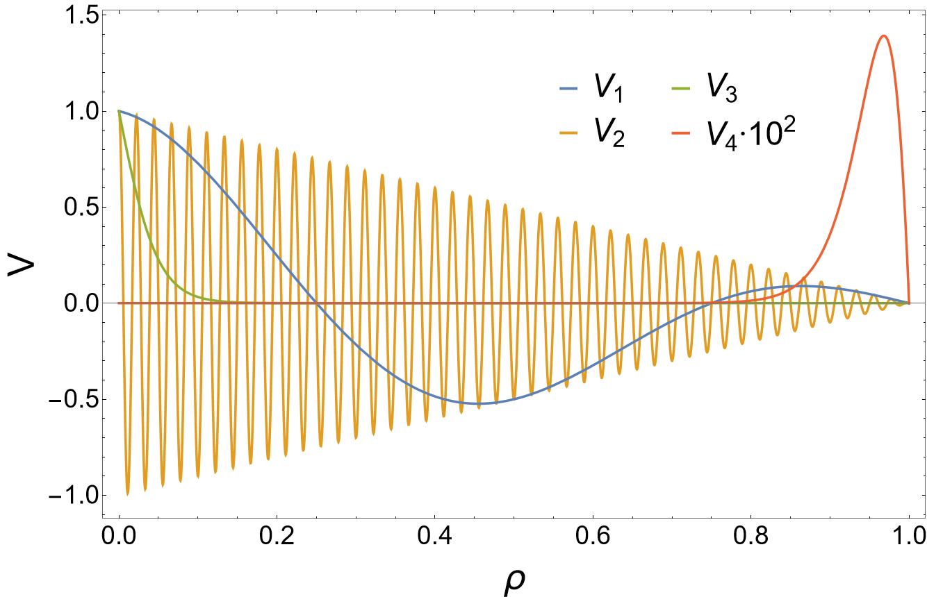
Refer to caption
Figure 3: Deterministic potentials (119) with Ai=1subscript𝐴𝑖1A_{i}=1. Recall that the horizon is at ρ=0𝜌0\rho=0 and the boundary at ρ=1𝜌1\rho=1.

Interestingly, for the pseudospectrum (both full and selective), the grid establishes a cutoff for the ρ𝜌\rho-wavelength of the perturbations. Thus, as a byproduct of the discretization, we are only truly sensitive to the stability under perturbations above the cutoff. Nonetheless, these grid effects are expected to be small; otherwise, the values of the QNFs would depend greatly on the grid and no numerical method would be reliable.

Finally, to stress the nontrivial nature of the norm, we also consider the pseudospectrum in the L2superscript𝐿2L^{2}-norm

uL2=𝑑ρu(𝓉,𝐤,ρ)u(𝓉,𝐤,ρ).subscriptnorm𝑢superscript𝐿2differential-d𝜌superscript𝑢𝓉𝐤𝜌𝑢𝓉𝐤𝜌\norm{u}_{L^{2}}=\int d\rho\,\,u^{*}(\mathscr{t},\mathbf{k},\rho)u(\mathscr{t},\mathbf{k},\rho)\,. (120)

Although the physical relevance of this norm for the present problem is less clear, it might be informative to compare the general features of the pseudospectra in the energy norm to those in the L2superscript𝐿2L^{2}-norm. We direct the interested reader to Appendix C where we present the pseudospectrum analysis in the L2superscript𝐿2L^{2}-norm.

6 Results

Here, we present the results of the analysis described in the previous sections. Our numerical simulations are performed in a grid of 120 points with a precision 5×5\timesMachinePrecision.

Refer to caption
(a) Scalar with m2l2=0superscript𝑚2superscript𝑙20m^{2}l^{2}=0 and 𝖖2=0superscript𝖖20\boldsymbol{\mathfrak{q}}^{2}=0.
Refer to caption
(b) Transverse Gauge Field with 𝖖2=0superscript𝖖20\boldsymbol{\mathfrak{q}}^{2}=0.
Figure 4: Convergence test for QNFs computed with 5×5\timesMachinePrecision. The error is defined as |1|𝔴||𝔴ref||1𝔴subscript𝔴ref\left|1-\frac{|\mathfrak{w}|}{|\mathfrak{w}_{\text{ref}}|}\right|, with 𝔴refsubscript𝔴ref\mathfrak{w}_{\text{ref}} the reference value obtained with 10×10\timesMachinePrecision in grid of 400400400 points. The missing points are such that their error is below the numerical accuracy.

It is important to note that we require large grids and high precision to ensure that the numerical procedure does not heavily affect our results. Physically, the discretization and numerical round-offs can be understood as perturbations to the original problem and, as we want to analyze the stability of the latter, we need to be especially careful and avoid undesired effects associated with them. As we are mainly interested in the stability of the three or four lowest-lying QNFs, in figure 4 we test the validity of our numerics by computing those QNFs in our setup and comparing them to the ones obtained using 10×10\timesMachinePrecision in a grid of 400 points.282828Henceforth, we abuse notation and denote by QNF the pair {𝔴,𝔴}𝔴superscript𝔴\{\mathfrak{w},-\mathfrak{w}^{*}\}. Note that, as the equations of motion are invariant under simultaneous conjugation and multiplication by 11-1, the spectrum (and pseudospectrum) is symmetric under reflections along the imaginary axis and consequently the eigenvalues always appear in pairs {𝔴,𝔴}𝔴superscript𝔴\{\mathfrak{w},-\mathfrak{w}^{*}\}. Furthermore, we choose to order the QNFs by their imaginary part such the first QNF is the one with the largest imaginary part. Thus, we conclude that with our choice of parameters, we are ensuring that the effect of the numerics on the first four QNFs is smaller than 1050superscript105010^{-50} in all cases. It is interesting to note that the need for such large grids and precisions is a good indicator of the underlying instability of the problem. Small perturbations associated with the numerics have effects much larger than their typical scale (see figure 5).
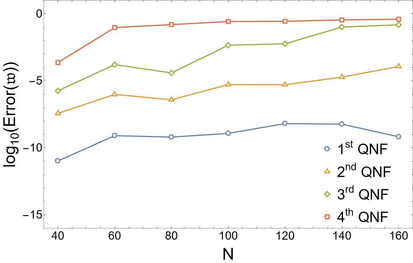
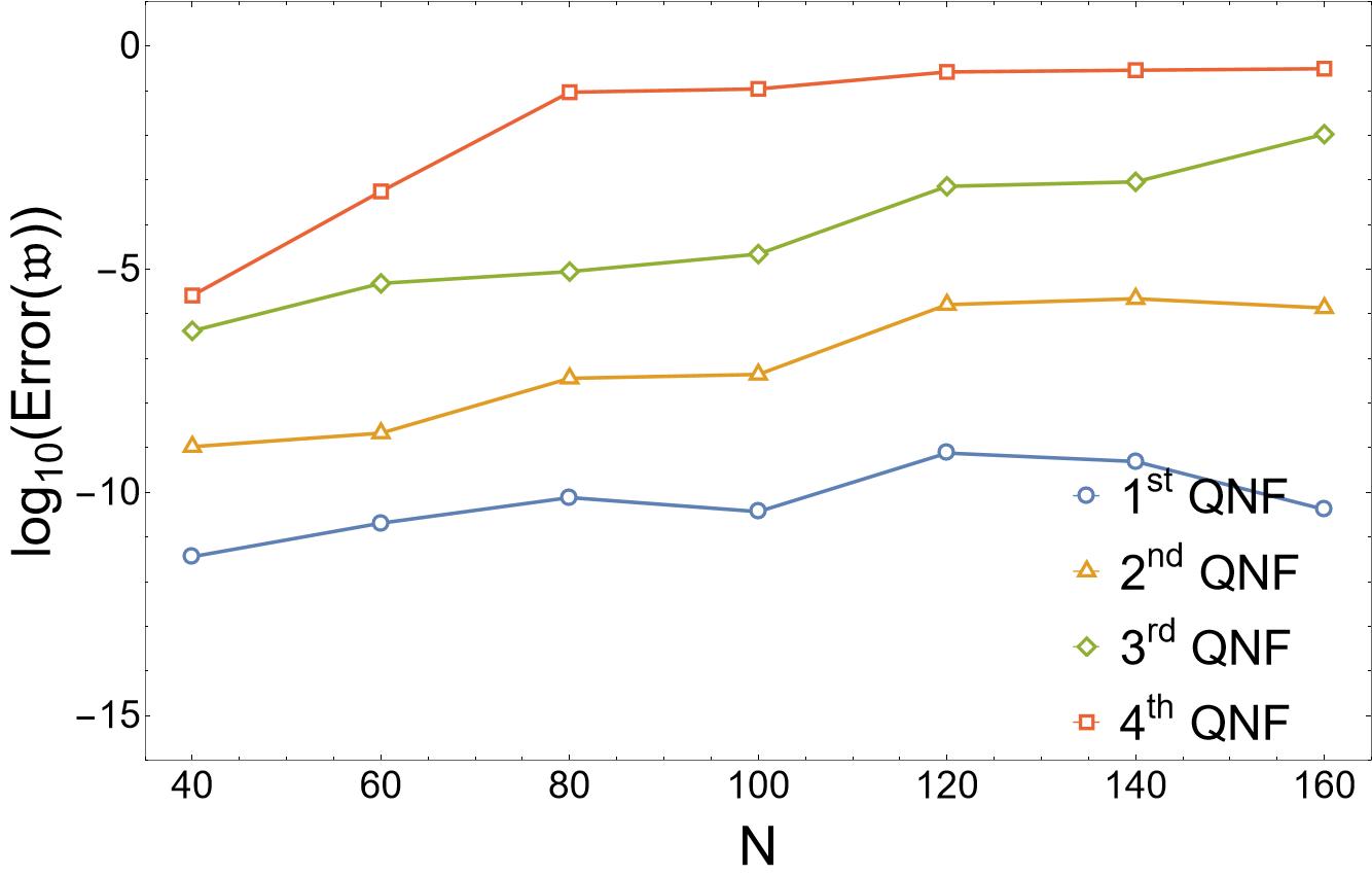
Refer to caption
(a) Scalar with m2l2=0superscript𝑚2superscript𝑙20m^{2}l^{2}=0 and 𝖖2=0superscript𝖖20\boldsymbol{\mathfrak{q}}^{2}=0.
Refer to caption
(b) Transverse Gauge Field with 𝖖2=0superscript𝖖20\boldsymbol{\mathfrak{q}}^{2}=0.
Figure 5: Convergence test for QNFs computed with MachinePrecision. The error is defined as |1|𝔴||𝔴ref||1𝔴subscript𝔴ref\left|1-\frac{|\mathfrak{w}|}{|\mathfrak{w}_{\text{ref}}|}\right|, with 𝔴refsubscript𝔴ref\mathfrak{w}_{\text{ref}} the reference value obtained with 10×10\timesMachinePrecision in grid of 400400400 points. The large error of the fourth QNF hints towards spectral instability.

6.1 Real Scalar in SAdS4+1subscriptSAdS41\text{SAdS}_{4+1}

Refer to caption
(a) m2l2=0superscript𝑚2superscript𝑙20m^{2}l^{2}=0, 𝔮=0𝔮0\mathfrak{q}=0.
Refer to caption
(b) m2l2=0superscript𝑚2superscript𝑙20m^{2}l^{2}=0, 𝔮=10𝔮10\mathfrak{q}=10.
Refer to caption
(c) m2l2=3superscript𝑚2superscript𝑙23m^{2}l^{2}=-3, 𝔮=0𝔮0\mathfrak{q}=0.
Refer to caption
(d) m2l2=3superscript𝑚2superscript𝑙23m^{2}l^{2}=-3, 𝔮=10𝔮10\mathfrak{q}=10.
Figure 6: Close-up of the scalar pseudospectrum in the energy norm around the first QNF for different values of 𝔮𝔮\mathfrak{q} and m2l2superscript𝑚2superscript𝑙2m^{2}l^{2}. The red dot corresponds to the QNF, the white lines represent the boundaries of various full ε𝜀\varepsilon-pseudospectra, and the dashed blue circle symbolizes a circle with a radius of 101superscript10110^{-1} centered on the QNF. The heat map corresponds to the logarithm in base 10 of the inverse of the resolvent, while the blue and cyan dots indicate selective ε𝜀\varepsilon-pseudospectra computed with random local potential perturbations of size 101superscript10110^{-1} and 103superscript10310^{-3}, respectively. Remarkably, only in (a) do we observe instability of the first QNF under local potential perturbations.

In figures 6 and 7, we present full and selective pseudospectra and the corresponding condition numbers in the energy norm for different values of m2l2superscript𝑚2superscript𝑙2m^{2}l^{2} and 𝔮=𝖖2𝔮superscript𝖖2\mathfrak{q}=\sqrt{\boldsymbol{\mathfrak{q}}^{2}}. Recall that throughout this section we are working in units of zh=(πT)1subscript𝑧superscript𝜋𝑇1z_{h}=(\pi\,T)^{-1}. The ε𝜀\varepsilon-pseudospectra exhibit extended open regions denoting instability.292929Note that all QNFs are contained within some region of the ε𝜀\varepsilon-pseudospectra. However, due to limited resolution in the plots, not all regions of the ε𝜀\varepsilon-pseudospectrum are observable. For example, in the full pseudospectrum shown in figure 7(a), we cannot appreciate the 107superscript10710^{-7}-pseudospectrum around the first QNF observable in figure 6(a). The same limitation applies to the selective pseudospectra, where small regions are covered by the red dots representing the QNFs (e.g., the selective 103superscript10310^{-3}-pseudospectrum observed around the first QNF in figure 6(a) is covered by a red dot in figure 7(a)). As observed in asymptotically flat Jaramillo:2020tuu ; Destounis:2021lum and de Sitter spacetimes Sarkar:2023rhp , the instability increases the further away the QNFs are from the real axis; which, for the dual quantum field theory, implies that excitations are progressively unstable the more short-lived they are.

Interestingly, we find that one needs perturbations of size 100.40.4similar-toabsentsuperscript100.4similar-to0.4\sim 10^{-0.4}\sim 0.4 to drive the QNFs to the upper half of the complex plane, as indicated by the full pseudospectra in figure 7. Noting that the typical distance between eigenvalues is 2similar-toabsent2\sim 2, this implies that all backgrounds arising as a small deviation from SAdS4+1 are stable, i.e., they do not have exponentially growing QNMs. For the dual QFT, this indicates that the ground state is stable despite the spectrum being unstable.
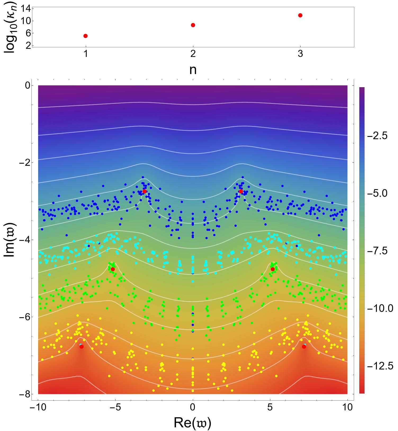
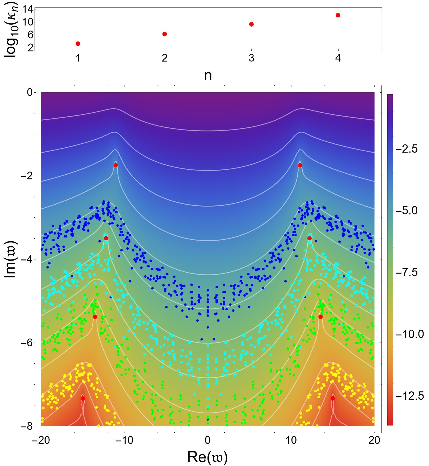
Refer to caption
(a) m2l2=0superscript𝑚2superscript𝑙20m^{2}l^{2}=0, 𝔮=0𝔮0\mathfrak{q}=0.
Refer to caption
(b) m2l2=0superscript𝑚2superscript𝑙20m^{2}l^{2}=0, 𝔮=10𝔮10\mathfrak{q}=10.
Refer to caption
(c) m2l2=3superscript𝑚2superscript𝑙23m^{2}l^{2}=-3, 𝔮=0𝔮0\mathfrak{q}=0.
Refer to caption
(d) m2l2=3superscript𝑚2superscript𝑙23m^{2}l^{2}=-3, 𝔮=10𝔮10\mathfrak{q}=10.
Figure 7: Scalar pseudospectrum in the energy norm for different values of 𝔮𝔮\mathfrak{q} and m2l2superscript𝑚2superscript𝑙2m^{2}l^{2}. In the lower panels, we present selective and full pseudospectra. The red dots represent the (unperturbed) QNFs in the typical “Christmas Tree” configuration. The white lines denote the boundaries of different full ε𝜀\varepsilon-pseudospectra. The heat map corresponds to the logarithm in base 10 of the inverse of the resolvent, while the blue, cyan, green, and yellow dots indicate different selective ε𝜀\varepsilon-pseudospectra computed with random local potential perturbations of size 101superscript10110^{-1}, 103superscript10310^{-3}, 105superscript10510^{-5}, and 107superscript10710^{-7}; respectively. In the upper panels, we represent the condition numbers. Most notably, for small values of ε𝜀\varepsilon, the full ε𝜀\varepsilon-pseudospectra present open regions containing multiple QNFs, which signals spectral instability.

Focusing now on the selective pseudospectrum, we note that its structure seems to resemble the structure of the full pseudospectrum. Nonetheless, the scales clearly do not match; the selective pseudospectrum shows significantly more stability. Hence, we can conclude that most of the instability arises from perturbations which cannot be interpreted as local potential perturbations.

Regarding the mass and momentum dependence, stability decreases with mass and increases with momentum (see figures 8 and 9). Such behaviour can be understood in the context of the instability being related to the distance to the real axis: the imaginary part of the QNFs is reduced as mass (momentum) decreases (increases), and thus we observe more stability. For the QFT this implies that high-momentum fluctuations of operators with small scaling dimension are more stable.
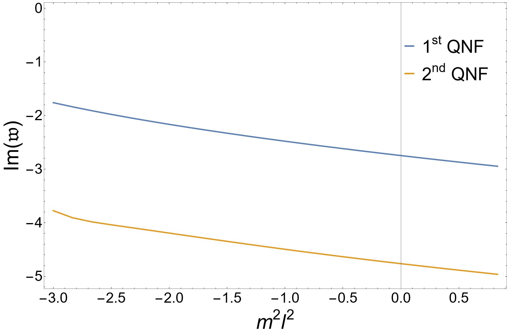
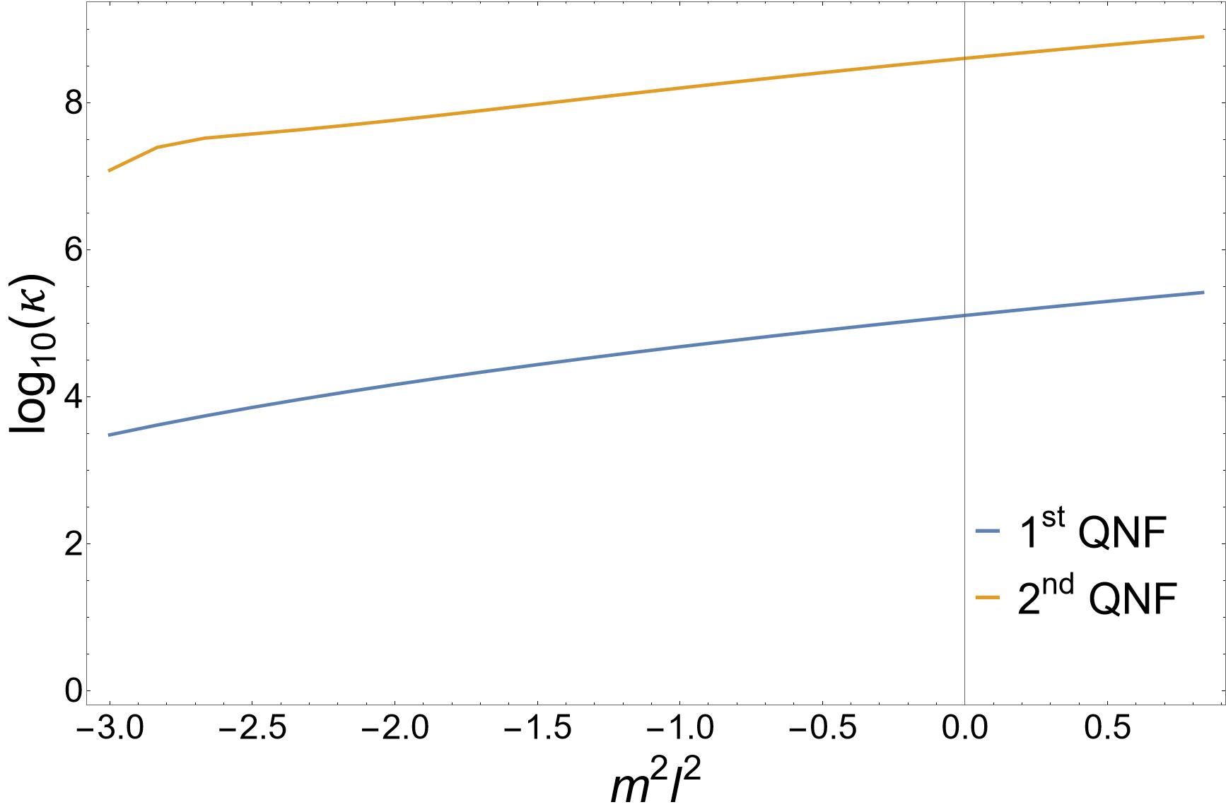
Refer to caption
(a) Imaginary part of the QNFs for 𝔮=0𝔮0\mathfrak{q}=0.
Refer to caption
(b) Condition numbers for 𝔮=0𝔮0\mathfrak{q}=0.
Refer to caption
(c) Imaginary part of the QNFs for 𝔮=10𝔮10\mathfrak{q}=10.
Refer to caption
(d) Condition numbers for 𝔮=10𝔮10\mathfrak{q}=10.
Figure 8: Mass dependence in the energy norm for the scalar fluctuations.
Refer to caption
(a) Imaginary part of the QNFs for m2l2=0superscript𝑚2superscript𝑙20m^{2}l^{2}=0.
Refer to caption
(b) Condition numbers for m2l2=0superscript𝑚2superscript𝑙20m^{2}l^{2}=0.
Refer to caption
(c) Imaginary part of the QNFs for m2l2=3superscript𝑚2superscript𝑙23m^{2}l^{2}=-3.
Refer to caption
(d) Condition numbers for m2l2=3superscript𝑚2superscript𝑙23m^{2}l^{2}=-3.
Figure 9: Momentum dependence in the energy norm for the scalar fluctuations.
Refer to caption
(a) m2l2=0superscript𝑚2superscript𝑙20m^{2}l^{2}=0, 𝔮=0𝔮0\mathfrak{q}=0.
Refer to caption
(b) m2l2=0superscript𝑚2superscript𝑙20m^{2}l^{2}=0, 𝔮=10𝔮10\mathfrak{q}=10.
Refer to caption
(c) m2l2=3superscript𝑚2superscript𝑙23m^{2}l^{2}=-3, 𝔮=0𝔮0\mathfrak{q}=0.
Refer to caption
(d) m2l2=3superscript𝑚2superscript𝑙23m^{2}l^{2}=-3, 𝔮=10𝔮10\mathfrak{q}=10.
Figure 10: Effect on the first scalar QNF of the deterministic perturbations (119) with size ViE=101subscriptnormsubscript𝑉𝑖𝐸superscript101\norm{V_{i}}_{E}=10^{-1}. The unperturbed QNF is shown in red, while the perturbed QNFs are depicted in blue. The dashed blue line represents the circle of radius 101superscript10110^{-1} centered in the unperturbed QNF. Remarkably, only for 𝔮=0𝔮0\mathfrak{q}=0 do we observe instability under near-horizon perturbations (V3subscript𝑉3V_{3}).
Refer to caption
(a) m2l2=0superscript𝑚2superscript𝑙20m^{2}l^{2}=0, 𝔮=0𝔮0\mathfrak{q}=0.
Refer to caption
(b) m2l2=0superscript𝑚2superscript𝑙20m^{2}l^{2}=0, 𝔮=10𝔮10\mathfrak{q}=10.
Refer to caption
(c) m2l2=3superscript𝑚2superscript𝑙23m^{2}l^{2}=-3, 𝔮=0𝔮0\mathfrak{q}=0.
Refer to caption
(d) m2l2=3superscript𝑚2superscript𝑙23m^{2}l^{2}=-3, 𝔮=10𝔮10\mathfrak{q}=10.
Figure 11: Effect on the spectrum of the scalar of the deterministic perturbations (119) with size ViE=101subscriptnormsubscript𝑉𝑖𝐸superscript101\norm{V_{i}}_{E}=10^{-1}. In the lower panels we present the spectra and in the upper ones the condition numbers for the lowest QNFs. The unperturbed QNFs are shown in red, while the perturbed ones are depicted in blue. The plotted region of the spectra is stable under long ρ𝜌\rho-wavelength perturbations (V1subscript𝑉1V_{1}) and near-boundary perturbations (V4subscript𝑉4V_{4}). Note also that, as indicated by the condition numbers, the perturbed QNFs associated with V2subscript𝑉2V_{2} and V3subscript𝑉3V_{3} are more stable than the unperturbed QNFs.

We now focus on the first QNF (see figure 6), which has the smallest imaginary part and thus dominates the low energy spectrum of the QFT. Remarkably, we find that for sufficiently large mass and small momentum, it is unstable under local potential perturbations as the selective ε𝜀\varepsilon-pseudospectra extends beyond the circle of radius ε𝜀\varepsilon centered around the QNF. To further explore the nature of this instability, in figure 10 we analyze the effect of the deterministic potential perturbations (119) to the first QNF. We observe that the instability is only present for near-horizon perturbations, concluding that it is mainly associated with deformations of the IR of the dual QFT. Moreover, we also find that, although we did not have statistical evidence in the selective pseudospectra, the first QNF is actually unstable under local potential perturbations for m2l2=3superscript𝑚2superscript𝑙23m^{2}l^{2}=-3 (figure 10(c)).

Continuing our exploration of the effect of the deterministic potentials, in figure 11 we present the spectrum and the condition numbers for the first 3 perturbed QNFs. We observe that large ρ𝜌\rho-wavelength (V1subscript𝑉1V_{1}) and near-boundary (V4subscript𝑉4V_{4}) perturbations have very little effect on the spectrum. On the other hand, short ρ𝜌\rho-wavelength (V2subscript𝑉2V_{2}) and near-horizon perturbations (V3subscript𝑉3V_{3}) displace the QNFs significantly, generating new branching structures. Remarkably, these perturbed QNFs are more stable than the unperturbed ones, indicating that the spectra of poles of Green’s functions in strongly coupled holographic field theories might have some preference for branching structures over the unperturbed "Christmas Tree" configuration.

We end this section by briefly addressing the results for the pseudospectrum of the scalar field in the L2superscript𝐿2L^{2}-norm. We refer the reader to Appendix C and here we simply point out that the pseudospectra are qualitatively similar to those in the energy norm. However, in the L2superscript𝐿2L^{2}-norm we find that the stability is enhanced under local potential perturbations and reduced under generic perturbations.

6.2 Transverse Gauge Field in SAdS4+1subscriptSAdS41\text{SAdS}_{4+1}
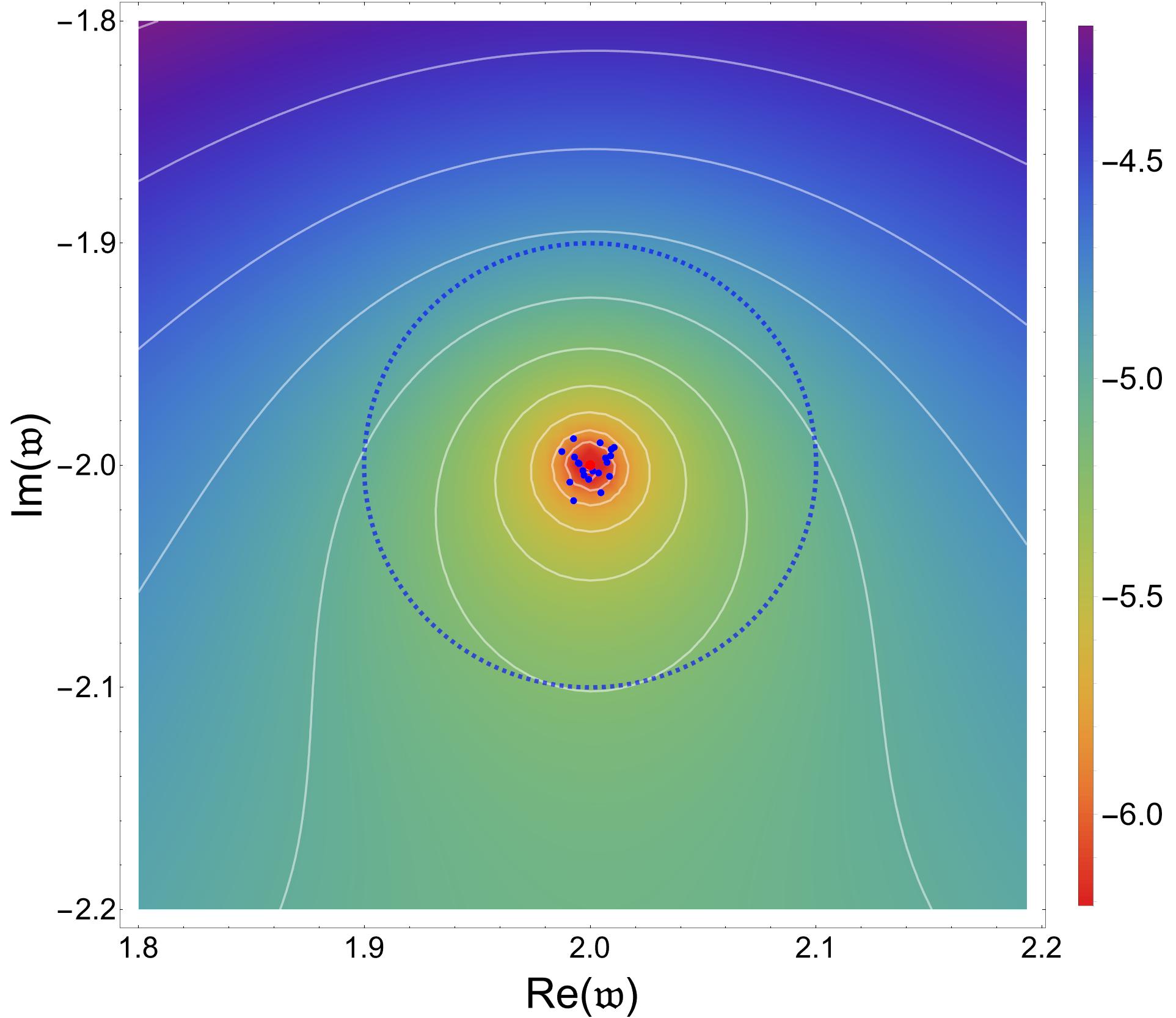
Refer to caption
(a) 𝔮=0𝔮0\mathfrak{q}=0.
Refer to caption
(b) 𝔮=10𝔮10\mathfrak{q}=10.
Figure 12: Close-up of the transverse gauge field pseudospectrum in the energy norm around the first QNF for different values of 𝔮𝔮\mathfrak{q}. The red dot corresponds to the QNF, the white lines represent the boundaries of various full ε𝜀\varepsilon-pseudospectra, and the dashed blue circle symbolizes a circle with a radius of 101superscript10110^{-1} centered on the QNF. The heat map corresponds to the logarithm in base 10 of the inverse of the resolvent, while the blue dots indicate selective ε𝜀\varepsilon-pseudospectra computed with random local potential perturbations.
Refer to caption
(a) 𝔮=0𝔮0\mathfrak{q}=0.
Refer to caption
(b) 𝔮=10𝔮10\mathfrak{q}=10.
Figure 13: Transverse gauge field pseudospectrum in the energy norm for different values of 𝔮𝔮\mathfrak{q}. In the lower panels, we present selective and full pseudospectra. The red dots represent the QNFs, and the white lines denote the boundaries of different full ε𝜀\varepsilon-pseudospectra. The heat map corresponds to the logarithm in base 10 of the inverse of the resolvent, while the blue, cyan, green, and yellow dots indicate different selective ε𝜀\varepsilon-pseudospectra computed with random local potential perturbations of size 101superscript10110^{-1}, 103superscript10310^{-3}, 105superscript10510^{-5}, and 107superscript10710^{-7}; respectively. In the upper panels, we represent the condition numbers.
Refer to caption
(a) 𝔮=0𝔮0\mathfrak{q}=0.
Refer to caption
(b) 𝔮=10𝔮10\mathfrak{q}=10.
Refer to caption
(c) 𝔮=0𝔮0\mathfrak{q}=0.
Refer to caption
(d) 𝔮=10𝔮10\mathfrak{q}=10.
Figure 14: Effect on the transverse gauge field spectrum of the deterministic perturbations (119) with size ViE=101subscriptnormsubscript𝑉𝑖𝐸superscript101\norm{V_{i}}_{E}=10^{-1}. The unperturbed QNF is shown in red, while the perturbed QNFs are depicted in blue. In (a) and (b) the dashed blue line represents the circle of radius 101superscript10110^{-1} centered in the unperturbed QNF. In the upper panels of (c) and (d) we present the condition numbers for the lowest QNFs.
Refer to caption
(a) Imaginary part of the QNFs.
Refer to caption
(b) Condition numbers.
Figure 15: Momentum dependence in the energy norm for the transverse gauge field.

In this section we present the pseudospectrum of the fluctuations of the transverse gauge field introduced in section 4.2. As we detail in the following, we observe the same generic features as for the real scalar. In particular we find the QNFs of the gauge field to be unstable.

First, in figures 12 and 13 we display the pseudospectrum of the transverse gauge field. The presence of open contour lines around the QNFs indicates that they are unstable under generic perturbations. However, for the first QNF we have not found statistical evidence of its instability under random local perturbations (see the selective pseudospectra in figure 12(a)). It is interesting to note that this is similar to what we found for the scalar field of mass m2l2=3superscript𝑚2superscript𝑙23m^{2}l^{2}=-3 (see figure 6(c)). From the conformal field theory point of view both of these fields correspond to operators of conformal dimension three.

In order to further characterize the nature of the instability, in figure 14 we show the effect of the deterministic perturbations (119) on the QNF spectrum. At zero momentum all QNFs we study are unstable under these perturbations. In particular in figure 14(a) the first QNF is shown to be unstable under near-horizon perturbations. Moreover, from studying the evolution of the condition numbers shown in that figure, one can conclude that near-horizon and short ρ𝜌\rho-wavelength perturbations result in less unstable QNFs.

As in the previous section it is also interesting to analyze the dependence of the stability of QNFs on the momentum of the fluctuation. Therefore, in figure 15 we plot the momentum dependence of the QNFs and their condition numbers. The QNFs get closer to the real axis as momentum increases, and, as for the real scalar, we observe that their condition numbers decrease in the process (although staying above one for the range of momentum studied).

Despite the qualitative similarities, it is worth noting that the actual values of the pseudospectra do not match the cases studied in the previous subsection. Specifically, we observe that the gauge field is more stable than the massless scalar and less stable than the scalar with mass m2l2=3superscript𝑚2superscript𝑙23m^{2}l^{2}=-3. This agrees with the instability being related to the imaginary part of the QNFs. The gauge field QNFs are closer to the real axis than those of the massless scalar and further away than those of the scalar with mass m2l2=3superscript𝑚2superscript𝑙23m^{2}l^{2}=-3.

Finally, it is illustrative to analyze the pseudospectrum in the L2superscript𝐿2L^{2}-norm. We present our results in appendix C. Again, we observe that in the L2superscript𝐿2L^{2}-norm we find the stability is enhanced under local potential perturbations and reduced under generic perturbations.

7 Conclusions

In this work we have initiated the study of the spectral stability of quasinormal modes in asymptotically AdS black hole geometries. Gauge/gravity duality maps the frequencies of those modes (QNFs) to the spectrum of collective excitations of a strongly coupled quantum many-body system. Therefore, probing the spectral stability of QNFs is akin to probing the stability of the spectra of strongly coupled holographic field theories.

Following previous works in asymptotically flat Jaramillo:2020tuu ; Destounis:2021lum and de Sitter spacetimes Sarkar:2023rhp , we probed spectral stability through pseudospectra and condition numbers. To construct the pseudospectra, we needed to choose a physically motivated norm and cast the equations of motion for the quasinormal modes in the form of an eigenvalue problem. Consequently, in section 3 we proposed a generic approach valid for static black brane backgrounds, a family of spacetimes very prominent in the literature. Our approach relied on two cornerstones. First, the regular coordinates, which enabled us to write the equations of motion as an eigenvalue problem while also translating outgoing boundary conditions to regularity conditions on the horizon. And second, the energy norm, which represents the physically relevant notion of size for the QNMs.

After discussing the general approach, we proceeded to study the stability of a real scalar field and a transverse gauge field in SAdS4+1. As previously observed in asymptotically flat Jaramillo:2020tuu ; Destounis:2021lum and dS spacetimes Sarkar:2023rhp , we found that the QNFs are unstable and that the instability is associated with the existence of a horizon. Moreover, we observed that QNFs are less unstable the closer they are to the real axis, a feature also present in the aforementioned spacetimes.

Regarding the scalar, we found an increase in stability at high momenta and small masses. This implies that in the dual QFT the instability is milder for high-momentum fluctuations of operators with small mass dimension. In order to further study the nature of the instability we probed the spectrum of QNFs with local potential perturbations, which could arise as effective interactions representing deviations from the exact SAdS4+1 background. Remarkably, we inferred that only a small portion of the total instability is associated with these perturbations. Moreover, we concluded that small perturbations cannot drive the QNFs to the upper half of the complex plane. We also found that for small momenta, the first QNF is unstable, with the instability arising from localized perturbations near the horizon. Thus, small deformations of the IR can destabilize even the lowest QNF.

With respect to the gauge field, we conclude that its pseudospectrum is qualitatively very similar to that of the scalar field. This is even more pronounced for the scalar of mass m2l2=3superscript𝑚2superscript𝑙23m^{2}l^{2}=-3. In that case both the scalar and the transverse gauge field correspond to operators with the same conformal dimension. Actually the resemblance between the pseudospectra of the scalar and the gauge field might be due to the fact that the spectra of both fields are very similar. Exploring this potential connection would indicate a degree of universality, which would be intriguing to investigate in future research.

We have proven that AdS spacetimes also present spectral instability associated with the existence of an event horizon. This supports the physical intuition that the observed instability is a direct consequence of the non-conservative character of black holes and thus is independent of the asymptotic behaviour of the spacetime.

With regard to gauge/gravity duality, our results imply that thermal excitation spectra of strongly coupled quantum field theories dual to SAdS4+1 (or some small deviation from it) are unstable. This suggests that a mathematical model would not be able to accurately represent the actual spectra of the real physical system. That said, it is important to remark that the instability decreases with the decay width of the fluctuations. We expect the imprint of the aforementioned instability to be less pronounced for modes near the real axis. We want to stress the importance of this result; in a practical setting it implies that, at most, one can hope to be able to capture the leading order behaviour (dominated by the longest-lived excitation). On the other hand it might not be possible to model the subleading features of decay trustfully as the higher QNFs are increasingly unstable.

The pseudospectral analysis in asymptotic AdS geometries has many applications, with potentially deep implications, in the realm of gauge/gravity duality. We list some of them in the following.

  • Study the stability of hydrodynamic modes. As we have seen, the closer a QNF is to the real axis, the less unstable it becomes. In particular that might indicate that hydrodynamic modes enjoy privileged stability properties in the pseudospectrum. On the other hand, if this effect is not sufficiently pronounced it would be interesting to see whether small local perturbations at zero momentum could drive the hydro mode’s QNF to the upper half plane indicating instabilities of flow patterns. In fact such instabilities have been argued to arise in Navier-Stokes equations and explain the early onset of turbulence trefethen1993hydrodynamic .

  • Study the stability of the collision between the hydro mode’s QNF and the first non-hydro mode’s QNF. This would shed a new perspective on the validity of the hydrodynamic approximation. Currently, the hydrodynamic expansion is postulated to be valid up to the energy where the aforementioned collision happens Withers:2018srf ; GrozdanovKovtun:2019 ; Grozdanov:2019 ; consequently, finding instability would indicate that the limit of validity itself is unstable. A similar comment applies to pole skipping points. These are points at which the residue of a QNM as pole of a holgraphic Green’s function vanishes Amado:2007yr ; Amado:2008ji . Such points are of particular interest in relation to quantum chaos Grozdanov:2017ajz ; Blake:2017ris ; Blake:2018leo .

  • Study the stability of the phase transition in the holographic superconductor model Hartnoll:2008vx . It would be interesting to see whether the critical temperature is stable under the generic perturbations captured by the pseudospectrum.

  • Study the spectral stability of AdS Reissner-Nordström black branes. The pseudospectrum analysis of charged black branes might have important consequences for the dual description of quantum critical phases of matter zaanen2015holographic ; Hartnoll:2018xxg .

  • Study the spectral stability of other solutions frequently used in holography. Beyond completing the current literature of QNFs in AdS spacetimes, it would be interesting to explore the existence of some degree of universality in the pseudospectrum. In particular, as spectra in AdS typically share the "Christmas Tree" structure observed in the current work (see, for instance, Kovtun:2005 ; Amado:2009ts ), this study would answer whether the overarching features observed here are fundamental to the structure of the spectrum or depend heavily on the particular setup.

  • It has recently been suggested that quasinormal modes can serve as a signature for having successfully simulated (quantum) gravity on a (quantum) computer Biggs:2023sqw ; Maldacena:2023acv . In view of our results this idea suffers from similar problems as the idea of black hole spectroscopy from gravitational wave signals. If such (quantum) simulations can be realized then the task of identifying the quasinormal modes will be subject to similar difficulties as for astrophysical black holes (see Jaramillo:2021tmt for a relevant discussion of this issue).

  • A different way of studying the poles of holographic Green’s functions is to look for complex solutions for the momenta upon fixing the frequency to be a real number Amado:2007pv . This is particularly important for the diffusive mode and has implications for causality Landsteiner:2012gn (see also the recent preprint Gavassino:2023mad ). It would be interesting to study the pseudospectra of these complex momentum modes.

Acknowledgements

The work of D.A and K.L. is supported through the grants CEX2020-001007-S and PID2021-123017NB-100, PID2021-127726NB-I00 funded by MCIN/AEI/10.13039/501100011033 and by ERDF “A way of making Europe". The work of D.G.F. is supported by JAEIntroICU-2022-IFT-02.

Appendix A Computation of Lsuperscript𝐿L^{\dagger}

Here we present a detailed computation of the adjoint operator Lsuperscript𝐿L^{\dagger} for the real scalar field (equation (103)) and transverse gauge field (equation (115)).

A.1 Real Scalar Field

For the real scalar field, the differential operator L𝐿L is given by

L=i(01L1[ρ2,ρ;𝖖,ρ]L2[ρ;𝖖,ρ]),𝐿𝑖matrix01subscript𝐿1superscriptsubscript𝜌2subscript𝜌𝖖𝜌subscript𝐿2subscript𝜌𝖖𝜌L=i\begin{pmatrix}0&1\\ L_{1}\left[\partial_{\mathscr{\rho}}^{2},\partial_{\mathscr{\rho}};\boldsymbol{\mathfrak{q}},\rho\right]&L_{2}\left[\partial_{\rho};\boldsymbol{\mathfrak{q}},\rho\right]\end{pmatrix}\,, (121)

with

L1[ρ2,ρ;𝖖,ρ]subscript𝐿1superscriptsubscript𝜌2subscript𝜌𝖖𝜌\displaystyle L_{1}\left[\partial_{\rho}^{2},\partial_{\rho};\boldsymbol{\mathfrak{q}},\rho\right] =[𝒻(ρ)2]1[m2l2(1ρ)2+𝖖2(1ρ)3(𝒻(ρ)(1ρ)3)ρ𝒻(ρ)ρ2],absentsuperscriptdelimited-[]𝒻𝜌21delimited-[]superscript𝑚2superscript𝑙2superscript1𝜌2superscript𝖖2superscript1𝜌3superscript𝒻𝜌superscript1𝜌3subscript𝜌𝒻𝜌superscriptsubscript𝜌2\displaystyle=\left[\mathscr{f}(\rho)-2\right]^{-1}\left[\frac{m^{2}l^{2}}{(1-\rho)^{2}}+\boldsymbol{\mathfrak{q}}^{2}-(1-\rho)^{3}\left(\frac{\mathscr{f}(\rho)}{(1-\rho)^{3}}\right)^{\prime}\partial_{\rho}-\mathscr{f}(\rho)\partial_{\rho}^{2}\right]\,, (122)
L2[ρ;𝖖,ρ]subscript𝐿2subscript𝜌𝖖𝜌\displaystyle L_{2}\left[\partial_{\rho};\boldsymbol{\mathfrak{q}},\rho\right] =[𝒻(ρ)2]1[(1ρ)3(𝒻(ρ)1(1ρ)3)+2(𝒻(ρ)1)ρ],absentsuperscriptdelimited-[]𝒻𝜌21delimited-[]superscript1𝜌3superscript𝒻𝜌1superscript1𝜌32𝒻𝜌1subscript𝜌\displaystyle=\left[\mathscr{f}(\rho)-2\right]^{-1}\left[(1-\rho)^{3}\left(\frac{\mathscr{f}(\rho)-1}{(1-\rho)^{3}}\right)^{\prime}+2\left(\mathscr{f}(\rho)-1\right)\partial_{\rho}\right]\,, (123)

and the inner product induced by the energy norm is:

ϕ1,ϕ2E=subscriptexpectation-valuesubscriptitalic-ϕ1subscriptitalic-ϕ2𝐸absent\displaystyle\expectationvalue{\phi_{1},\phi_{2}}_{E}= 01dρ(1ρ)3[(m2l2(1ρ)2+𝖖2)ϕ1¯(𝓉,𝐤,ρ)ϕ2(𝓉,𝐤,ρ)+\displaystyle\int_{0}^{1}\frac{d\rho}{(1-\rho)^{3}}\Biggl{[}\left(\frac{m^{2}l^{2}}{(1-\rho)^{2}}+\boldsymbol{\mathfrak{q}}^{2}\right)\overline{\phi_{1}}(\mathscr{t},\mathbf{k},\rho)\phi_{2}(\mathscr{t},\mathbf{k},\rho)+
+𝒻(ρ)ρϕ1¯(𝓉,𝐤,ρ)ρϕ2(𝓉,𝐤,ρ)(𝒻(ρ)2)ψ1¯(𝓉,𝐤,ρ)ψ2(𝓉,𝐤,ρ)].\displaystyle+\mathscr{f}(\rho)\partial_{\rho}\overline{\phi_{1}}(\mathscr{t},\mathbf{k},\rho)\partial_{\rho}\phi_{2}(\mathscr{t},\mathbf{k},\rho)-\left(\mathscr{f}(\rho)-2\right)\overline{\psi_{1}}(\mathscr{t},\mathbf{k},\rho)\psi_{2}(\mathscr{t},\mathbf{k},\rho)\Biggr{]}\,. (124)

For notational convenience, we drop the explicit dependence of all functions and denote ρ𝜌\rho derivatives with a prime.

Now, recalling the equality:

L[ϕ1],ϕ2E=ϕ1,L[ϕ2]E,subscriptexpectation-valuesuperscript𝐿delimited-[]subscriptitalic-ϕ1subscriptitalic-ϕ2𝐸subscriptexpectation-valuesubscriptitalic-ϕ1𝐿delimited-[]subscriptitalic-ϕ2𝐸\expectationvalue{L^{\dagger}\left[\phi_{1}\right],\phi_{2}}_{E}=\expectationvalue{\phi_{1},L\left[\phi_{2}\right]}_{E}\,, (125)

we can compute Lsuperscript𝐿L^{\dagger} integrating by parts

ϕ1,L[ϕ2]E=subscriptexpectation-valuesubscriptitalic-ϕ1𝐿delimited-[]subscriptitalic-ϕ2𝐸absent\displaystyle\expectationvalue{\phi_{1},L\left[\phi_{2}\right]}_{E}= i01dρ(1ρ)3[(m2l2(1ρ)2+𝖖2)ϕ1¯ψ2+ϕ1¯𝒻ψ2ψ1¯{(m2l2(1ρ)2+𝖖2)ϕ2\displaystyle\,i\int_{0}^{1}\frac{d\rho}{(1-\rho)^{3}}\Biggl{[}\left(\frac{m^{2}l^{2}}{(1-\rho)^{2}}+\boldsymbol{\mathfrak{q}}^{2}\right)\overline{\phi_{1}}\psi_{2}+\overline{\phi_{1}}^{\prime}\mathscr{f}\psi_{2}^{\prime}-\overline{\psi_{1}}\left\{\left(\frac{m^{2}l^{2}}{(1-\rho)^{2}}+\boldsymbol{\mathfrak{q}}^{2}\right)\phi_{2}\right.
(1ρ)3(𝒻ϕ2(1ρ)3)+(1ρ)3((𝒻1)ψ2(1ρ)3)+(𝒻1)ψ2}]\displaystyle\left.-(1-\rho)^{3}\left(\frac{\mathscr{f}\phi_{2}^{\prime}}{(1-\rho)^{3}}\right)^{\prime}+(1-\rho)^{3}\left(\frac{(\mathscr{f}-1)\psi_{2}}{(1-\rho)^{3}}\right)^{\prime}+\left(\mathscr{f}-1\right)\psi_{2}^{\prime}\right\}\Biggr{]}
=\displaystyle= i01dρ(1ρ)3[(m2l2(1ρ)2+𝖖2)ϕ2ψ1¯+ϕ2𝒻ψ1¯ψ2{(m2l2(1ρ)2+𝖖2)ϕ1¯\displaystyle-i\int_{0}^{1}\frac{d\rho}{(1-\rho)^{3}}\Biggl{[}\left(\frac{m^{2}l^{2}}{(1-\rho)^{2}}+\boldsymbol{\mathfrak{q}}^{2}\right)\phi_{2}\overline{\psi_{1}}+\phi_{2}^{\prime}\mathscr{f}\overline{\psi_{1}}^{\prime}-\psi_{2}\left\{\left(\frac{m^{2}l^{2}}{(1-\rho)^{2}}+\boldsymbol{\mathfrak{q}}^{2}\right)\overline{\phi_{1}}\right.
(1ρ)3(𝒻ϕ1¯(1ρ)3)+(1ρ)3((𝒻1)ψ1¯(1ρ)3)+(𝒻1)ψ1¯}]\displaystyle\left.-(1-\rho)^{3}\left(\frac{\mathscr{f}\overline{\phi_{1}}^{\prime}}{(1-\rho)^{3}}\right)^{\prime}+(1-\rho)^{3}\left(\frac{(\mathscr{f}-1)\overline{\psi_{1}}}{(1-\rho)^{3}}\right)^{\prime}+\left(\mathscr{f}-1\right)\overline{\psi_{1}}^{\prime}\right\}\Biggr{]}
+i𝒻ϕ1¯ψ2(1ρ)3|ρ=0ρ=1+i𝒻ψ1¯ϕ2(1ρ)3|ρ=0ρ=12i(𝒻1)ψ1¯ψ2(1ρ)3|ρ=0ρ=1evaluated-at𝑖𝒻superscript¯subscriptitalic-ϕ1subscript𝜓2superscript1𝜌3𝜌0𝜌1evaluated-at𝑖𝒻¯subscript𝜓1superscriptsubscriptitalic-ϕ2superscript1𝜌3𝜌0𝜌1evaluated-at2𝑖𝒻1¯subscript𝜓1subscript𝜓2superscript1𝜌3𝜌0𝜌1\displaystyle+\left.i\frac{\mathscr{f}\overline{\phi_{1}}^{\prime}\psi_{2}}{(1-\rho)^{3}}\right|_{\rho=0}^{\rho=1}+\left.i\frac{\mathscr{f}\overline{\psi_{1}}\phi_{2}^{\prime}}{(1-\rho)^{3}}\right|_{\rho=0}^{\rho=1}-\left.2i\frac{(\mathscr{f}-1)\overline{\psi_{1}}\psi_{2}}{(1-\rho)^{3}}\right|_{\rho=0}^{\rho=1}
=\displaystyle= L[ϕ1],ϕ2E+i𝒻ϕ1¯ψ2(1ρ)3|ρ=0ρ=1+i𝒻ψ1¯ϕ2(1ρ)3|ρ=0ρ=12i(𝒻1)ψ1¯ψ2(1ρ)3|ρ=0ρ=1subscriptexpectation-value𝐿delimited-[]subscriptitalic-ϕ1subscriptitalic-ϕ2𝐸evaluated-at𝑖𝒻superscript¯subscriptitalic-ϕ1subscript𝜓2superscript1𝜌3𝜌0𝜌1evaluated-at𝑖𝒻¯subscript𝜓1superscriptsubscriptitalic-ϕ2superscript1𝜌3𝜌0𝜌1evaluated-at2𝑖𝒻1¯subscript𝜓1subscript𝜓2superscript1𝜌3𝜌0𝜌1\displaystyle\expectationvalue{L\left[\phi_{1}\right],\phi_{2}}_{E}+\left.i\frac{\mathscr{f}\overline{\phi_{1}}^{\prime}\psi_{2}}{(1-\rho)^{3}}\right|_{\rho=0}^{\rho=1}+\left.i\frac{\mathscr{f}\overline{\psi_{1}}\phi_{2}^{\prime}}{(1-\rho)^{3}}\right|_{\rho=0}^{\rho=1}-\left.2i\frac{(\mathscr{f}-1)\overline{\psi_{1}}\psi_{2}}{(1-\rho)^{3}}\right|_{\rho=0}^{\rho=1}
=\displaystyle= L[ϕ1],ϕ2E.subscriptexpectation-valuesuperscript𝐿delimited-[]subscriptitalic-ϕ1subscriptitalic-ϕ2𝐸\displaystyle\expectationvalue{L^{\dagger}\left[\phi_{1}\right],\phi_{2}}_{E}\,. (126)

The boundary terms vanish for ρ=1𝜌1\rho=1 as the chosen function space satisfies the boundary condition (101). However at ρ=0𝜌0\rho=0, we have 𝒻(0)=0𝒻00\mathscr{f}(0)=0, and we get a non-zero contribution arising from the last term. Then, the final expression for (A.1) is given by:

ϕ1,L[ϕ2]E=subscriptexpectation-valuesubscriptitalic-ϕ1𝐿delimited-[]subscriptitalic-ϕ2𝐸absent\displaystyle\expectationvalue{\phi_{1},L\left[\phi_{2}\right]}_{E}= L[ϕ1],ϕ2E2i(𝒻1)ψ1¯ψ2(1ρ)3|ρ=0subscriptexpectation-value𝐿delimited-[]subscriptitalic-ϕ1subscriptitalic-ϕ2𝐸evaluated-at2𝑖𝒻1¯subscript𝜓1subscript𝜓2superscript1𝜌3𝜌0\displaystyle\expectationvalue{L\left[\phi_{1}\right],\phi_{2}}_{E}-\left.2i\frac{(\mathscr{f}-1)\overline{\psi_{1}}\psi_{2}}{(1-\rho)^{3}}\right|_{\rho=0}
=\displaystyle= L[ϕ1],ϕ2Ei01dρ(1ρ)3(𝒻2)[2δ(ρ)𝒻(ρ)1𝒻(ρ)2]ψ1¯ψ2subscriptexpectation-value𝐿delimited-[]subscriptitalic-ϕ1subscriptitalic-ϕ2𝐸𝑖superscriptsubscript01𝑑𝜌superscript1𝜌3𝒻2delimited-[]2𝛿𝜌𝒻𝜌1𝒻𝜌2¯subscript𝜓1subscript𝜓2\displaystyle\expectationvalue{L\left[\phi_{1}\right],\phi_{2}}_{E}-i\int_{0}^{1}\frac{d\rho}{(1-\rho)^{3}}(\mathscr{f}-2)\left[2\delta(\rho)\frac{\mathscr{f}(\rho)-1}{\mathscr{f}(\rho)-2}\right]\overline{\psi_{1}}\psi_{2}
=\displaystyle= L[ϕ1],ϕ2E+δL[ϕ1],ϕ2E=L[ϕ1],ϕ2E,subscriptexpectation-value𝐿delimited-[]subscriptitalic-ϕ1subscriptitalic-ϕ2𝐸subscriptexpectation-value𝛿𝐿delimited-[]subscriptitalic-ϕ1subscriptitalic-ϕ2𝐸subscriptexpectation-valuesuperscript𝐿delimited-[]subscriptitalic-ϕ1subscriptitalic-ϕ2𝐸\displaystyle\expectationvalue{L\left[\phi_{1}\right],\phi_{2}}_{E}+\expectationvalue{\delta L\left[\phi_{1}\right],\phi_{2}}_{E}=\expectationvalue{L^{\dagger}\left[\phi_{1}\right],\phi_{2}}_{E}\,, (127)

from where we recover the expression for the adjoint given in equation (103):

L=L+δL=L+(0002iδ(ρ)𝒻(ρ)1𝒻(ρ)2).superscript𝐿𝐿𝛿𝐿𝐿matrix0002𝑖𝛿𝜌𝒻𝜌1𝒻𝜌2L^{\dagger}=L+\delta L=L+\begin{pmatrix}0&0\\[6.0pt] 0&-2i\delta(\rho)\frac{\mathscr{f}(\rho)-1}{\mathscr{f}(\rho)-2}\end{pmatrix}\,. (128)

A.2 Transverse Gauge Field

For the transverse gauge field, the differential operator L𝐿L is given by

L=i(01L1[ρ2,ρ;𝖖,ρ]L2[ρ;𝖖,ρ]),𝐿𝑖matrix01subscript𝐿1superscriptsubscript𝜌2subscript𝜌𝖖𝜌subscript𝐿2subscript𝜌𝖖𝜌L=i\begin{pmatrix}0&1\\ L_{1}\left[\partial_{\mathscr{\rho}}^{2},\partial_{\mathscr{\rho}};\boldsymbol{\mathfrak{q}},\rho\right]&L_{2}\left[\partial_{\rho};\boldsymbol{\mathfrak{q}},\rho\right]\end{pmatrix}\,, (129)

with

L1[ρ2,ρ;𝖖,ρ]subscript𝐿1superscriptsubscript𝜌2subscript𝜌𝖖𝜌\displaystyle L_{1}\left[\partial_{\rho}^{2},\partial_{\rho};\boldsymbol{\mathfrak{q}},\rho\right] =[𝒻(ρ)2]1[𝖖2(1ρ)(𝒻(ρ)1ρ)ρ𝒻(ρ)ρ2],absentsuperscriptdelimited-[]𝒻𝜌21delimited-[]superscript𝖖21𝜌superscript𝒻𝜌1𝜌subscript𝜌𝒻𝜌superscriptsubscript𝜌2\displaystyle=\left[\mathscr{f}(\rho)-2\right]^{-1}\left[\boldsymbol{\mathfrak{q}}^{2}-(1-\rho)\left(\frac{\mathscr{f}(\rho)}{1-\rho}\right)^{\prime}\partial_{\rho}-\mathscr{f}(\rho)\partial_{\rho}^{2}\right]\,, (130)
L2[ρ;𝖖,ρ]subscript𝐿2subscript𝜌𝖖𝜌\displaystyle L_{2}\left[\partial_{\rho};\boldsymbol{\mathfrak{q}},\rho\right] =[𝒻(ρ)2]1[(1ρ)(𝒻(ρ)1(1ρ))+2(𝒻(ρ)1)ρ],absentsuperscriptdelimited-[]𝒻𝜌21delimited-[]1𝜌superscript𝒻𝜌11𝜌2𝒻𝜌1subscript𝜌\displaystyle=\left[\mathscr{f}(\rho)-2\right]^{-1}\left[(1-\rho)\left(\frac{\mathscr{f}(\rho)-1}{(1-\rho)}\right)^{\prime}+2\left(\mathscr{f}(\rho)-1\right)\partial_{\rho}\right]\,, (131)

and the inner product induced by the energy norm is:

a1,a2E=subscriptexpectation-valuesubscript𝑎1subscript𝑎2𝐸absent\displaystyle\expectationvalue{a_{1},a_{2}}_{E}= 01dρ(1ρ)[𝖖2a1¯(𝓉,𝐤,ρ)a2(𝓉,𝐤,ρ)+𝒻(ρ)ρa1¯(𝓉,𝐤,ρ)ρa2(𝓉,𝐤,ρ)\displaystyle\int_{0}^{1}\frac{d\rho}{(1-\rho)}\Bigl{[}\boldsymbol{\mathfrak{q}}^{2}\overline{a_{1}}(\mathscr{t},\mathbf{k},\rho)a_{2}(\mathscr{t},\mathbf{k},\rho)+\mathscr{f}(\rho)\partial_{\rho}\overline{a_{1}}(\mathscr{t},\mathbf{k},\rho)\partial_{\rho}a_{2}(\mathscr{t},\mathbf{k},\rho)
(𝒻(ρ)2)α1¯(𝓉,𝐤,ρ)α2(𝓉,𝐤,ρ)].\displaystyle-\left(\mathscr{f}(\rho)-2\right)\overline{\alpha_{1}}(\mathscr{t},\mathbf{k},\rho)\alpha_{2}(\mathscr{t},\mathbf{k},\rho)\Bigr{]}\,. (132)

As with the scalar, we drop the explicit dependence of all functions and denote ρ𝜌\rho derivatives with a prime and compute Lsuperscript𝐿L^{\dagger} integrating by parts:

a1,L[a2]E=subscriptexpectation-valuesubscript𝑎1𝐿delimited-[]subscript𝑎2𝐸absent\displaystyle\expectationvalue{a_{1},L\left[a_{2}\right]}_{E}= i01dρ(1ρ)3[𝖖2a1¯α2+a1¯𝒻α2α1¯{𝖖2a2(1ρ)(𝒻a2(1ρ))\displaystyle i\int_{0}^{1}\frac{d\rho}{(1-\rho)^{3}}\Biggl{[}\boldsymbol{\mathfrak{q}}^{2}\overline{a_{1}}\alpha_{2}+\overline{a_{1}}^{\prime}\mathscr{f}\alpha_{2}^{\prime}-\overline{\alpha_{1}}\left\{\boldsymbol{\mathfrak{q}}^{2}a_{2}-(1-\rho)\left(\frac{\mathscr{f}a_{2}^{\prime}}{(1-\rho)}\right)^{\prime}\right.
+(1ρ)((𝒻1)α2(1ρ))+(𝒻1)α2}]\displaystyle\left.+(1-\rho)\left(\frac{(\mathscr{f}-1)\alpha_{2}}{(1-\rho)}\right)^{\prime}+\left(\mathscr{f}-1\right)\alpha_{2}^{\prime}\right\}\Biggr{]}
=\displaystyle= i01dρ(1ρ)3[𝖖2a2α1¯+a2𝒻α1α2{𝖖2a1¯(1ρ)(𝒻a1¯(1ρ))\displaystyle-i\int_{0}^{1}\frac{d\rho}{(1-\rho)^{3}}\Biggl{[}\boldsymbol{\mathfrak{q}}^{2}a_{2}\overline{\alpha_{1}}+a_{2}^{\prime}\mathscr{f}\alpha_{1}^{\prime}-\alpha_{2}\left\{\boldsymbol{\mathfrak{q}}^{2}\overline{a_{1}}-(1-\rho)\left(\frac{\mathscr{f}\overline{a_{1}}^{\prime}}{(1-\rho)}\right)^{\prime}\right.
+(1ρ)((𝒻1)α1¯(1ρ))+(𝒻1)α1¯}]\displaystyle\left.+(1-\rho)\left(\frac{(\mathscr{f}-1)\overline{\alpha_{1}}}{(1-\rho)}\right)^{\prime}+\left(\mathscr{f}-1\right)\overline{\alpha_{1}}^{\prime}\right\}\Biggr{]}
+i𝒻a1¯α2(1ρ)|ρ=0ρ=1+i𝒻α1¯a2(1ρ)|ρ=0ρ=12i(𝒻1)α1¯α2(1ρ)|ρ=0ρ=1evaluated-at𝑖𝒻superscript¯subscript𝑎1subscript𝛼21𝜌𝜌0𝜌1evaluated-at𝑖𝒻¯subscript𝛼1superscriptsubscript𝑎21𝜌𝜌0𝜌1evaluated-at2𝑖𝒻1¯subscript𝛼1subscript𝛼21𝜌𝜌0𝜌1\displaystyle+\left.i\frac{\mathscr{f}\overline{a_{1}}^{\prime}\alpha_{2}}{(1-\rho)}\right|_{\rho=0}^{\rho=1}+\left.i\frac{\mathscr{f}\overline{\alpha_{1}}a_{2}^{\prime}}{(1-\rho)}\right|_{\rho=0}^{\rho=1}-\left.2i\frac{(\mathscr{f}-1)\overline{\alpha_{1}}\alpha_{2}}{(1-\rho)}\right|_{\rho=0}^{\rho=1}
=\displaystyle= L[a1],a2E+i𝒻a1¯α2(1ρ)|ρ=0ρ=1+i𝒻α1¯a2(1ρ)|ρ=0ρ=12i(𝒻1)α1¯α2(1ρ)|ρ=0ρ=1subscriptexpectation-value𝐿delimited-[]subscript𝑎1subscript𝑎2𝐸evaluated-at𝑖𝒻superscript¯subscript𝑎1subscript𝛼21𝜌𝜌0𝜌1evaluated-at𝑖𝒻¯subscript𝛼1superscriptsubscript𝑎21𝜌𝜌0𝜌1evaluated-at2𝑖𝒻1¯subscript𝛼1subscript𝛼21𝜌𝜌0𝜌1\displaystyle\expectationvalue{L\left[a_{1}\right],a_{2}}_{E}+\left.i\frac{\mathscr{f}\overline{a_{1}}^{\prime}\alpha_{2}}{(1-\rho)}\right|_{\rho=0}^{\rho=1}+\left.i\frac{\mathscr{f}\overline{\alpha_{1}}a_{2}^{\prime}}{(1-\rho)}\right|_{\rho=0}^{\rho=1}-\left.2i\frac{(\mathscr{f}-1)\overline{\alpha_{1}}\alpha_{2}}{(1-\rho)}\right|_{\rho=0}^{\rho=1}
=\displaystyle= L[a1],a2E.subscriptexpectation-valuesuperscript𝐿delimited-[]subscript𝑎1subscript𝑎2𝐸\displaystyle\expectationvalue{L^{\dagger}\left[a_{1}\right],a_{2}}_{E}\,. (133)

The boundary terms vanish for ρ=1𝜌1\rho=1 as the chosen function space satisfies the boundary condition (113). Nonetheless, at ρ=0𝜌0\rho=0, we have 𝒻(0)=0𝒻00\mathscr{f}(0)=0, and we get a non-zero contribution arising from the last term. Then, the final expression for (A.2) is given by:

a1,L[a2]E=subscriptexpectation-valuesubscript𝑎1𝐿delimited-[]subscript𝑎2𝐸absent\displaystyle\expectationvalue{a_{1},L\left[a_{2}\right]}_{E}= L[a1],a2Ei01dρ(1ρ)(𝒻2)[2δ(ρ)𝒻(ρ)1𝒻(ρ)2]α1¯α2subscriptexpectation-value𝐿delimited-[]subscript𝑎1subscript𝑎2𝐸𝑖superscriptsubscript01𝑑𝜌1𝜌𝒻2delimited-[]2𝛿𝜌𝒻𝜌1𝒻𝜌2¯subscript𝛼1subscript𝛼2\displaystyle\expectationvalue{L\left[a_{1}\right],a_{2}}_{E}-i\int_{0}^{1}\frac{d\rho}{(1-\rho)}(\mathscr{f}-2)\left[2\delta(\rho)\frac{\mathscr{f}(\rho)-1}{\mathscr{f}(\rho)-2}\right]\overline{\alpha_{1}}\alpha_{2}
=\displaystyle= L[a1],a2E+δL[a1],a2E=L[a1],a2E,subscriptexpectation-value𝐿delimited-[]subscript𝑎1subscript𝑎2𝐸subscriptexpectation-value𝛿𝐿delimited-[]subscript𝑎1subscript𝑎2𝐸subscriptexpectation-valuesuperscript𝐿delimited-[]subscript𝑎1subscript𝑎2𝐸\displaystyle\expectationvalue{L\left[a_{1}\right],a_{2}}_{E}+\expectationvalue{\delta L\left[a_{1}\right],a_{2}}_{E}=\expectationvalue{L^{\dagger}\left[a_{1}\right],a_{2}}_{E}\,, (134)

from where we recover the expression for the adjoint given in equation (115):

L=L+δL=L+(0002iδ(ρ)𝒻(ρ)1𝒻(ρ)2).superscript𝐿𝐿𝛿𝐿𝐿matrix0002𝑖𝛿𝜌𝒻𝜌1𝒻𝜌2L^{\dagger}=L+\delta L=L+\begin{pmatrix}0&0\\[6.0pt] 0&-2i\delta(\rho)\frac{\mathscr{f}(\rho)-1}{\mathscr{f}(\rho)-2}\end{pmatrix}\,. (135)

Appendix B Discretization in the Chebyshev grid

In this section we give some more details regarding the discretization process. This discussion is based on the appendix C of Jaramillo:2020tuu .

B.1 Collocation Method

Working in the Chebyshev grid (116) with N+1𝑁1N+1 points is equivalent to approximating a function f(ρ)𝑓𝜌f(\rho) by a power series

f(ρ)n=0NcnTn(2ρ1),𝑓𝜌superscriptsubscript𝑛0𝑁subscript𝑐𝑛subscript𝑇𝑛2𝜌1f(\rho)\approx\sum_{n=0}^{N}c_{n}T_{n}(2\rho-1)\,, (136)

where Tnsubscript𝑇𝑛T_{n} are the Chebyshev polynomials

Tn(x)=cos(narccos(x)).subscript𝑇𝑛𝑥𝑛arccosine𝑥T_{n}(x)=\cos\left(n\arccos\left(x\right)\right)\,. (137)

However, in the numerical method we do not work with the coefficients {cn}subscript𝑐𝑛\{c_{n}\} but instead with the values of f(ρ)𝑓𝜌f(\rho) in the points of the grid (116). In order to connect both descriptions, we note that in our grid we have the following orthogonality relation

01dρ1(2ρ1)2Tm(2ρ1)Tn(2ρ1)superscriptsubscript01𝑑𝜌1superscript2𝜌12subscript𝑇𝑚2𝜌1subscript𝑇𝑛2𝜌1\displaystyle\int_{0}^{1}\frac{d\rho}{\sqrt{1-(2\rho-1)^{2}}}\,\,T_{m}(2\rho-1)T_{n}(2\rho-1) =π01𝑑θTm(cos(θπ))Tn(cos(θπ))absent𝜋superscriptsubscript01differential-d𝜃subscript𝑇𝑚𝜃𝜋subscript𝑇𝑛𝜃𝜋\displaystyle=\pi\int_{0}^{1}d\theta\,\,T_{m}\left(\cos(\theta\pi)\right)T_{n}\left(\cos(\theta\pi)\right)
πNj=0NTm(cos(jπN))Tn(cos(jπN))1+δj0+δjNabsent𝜋𝑁superscriptsubscript𝑗0𝑁subscript𝑇𝑚𝑗𝜋𝑁subscript𝑇𝑛𝑗𝜋𝑁1subscript𝛿𝑗0subscript𝛿𝑗𝑁\displaystyle\approx\frac{\pi}{N}\sum_{j=0}^{N}\frac{T_{m}\left(\cos\left(\frac{j\pi}{N}\right)\right)T_{n}\left(\cos\left(\frac{j\pi}{N}\right)\right)}{1+\delta_{j0}+\delta_{jN}}
=πNj=0NTm(2ρj1)Tn(2ρj1)1+δj0+δjNabsent𝜋𝑁superscriptsubscript𝑗0𝑁subscript𝑇𝑚2subscript𝜌𝑗1subscript𝑇𝑛2subscript𝜌𝑗11subscript𝛿𝑗0subscript𝛿𝑗𝑁\displaystyle=\frac{\pi}{N}\sum_{j=0}^{N}\frac{T_{m}\left(2\rho_{j}-1\right)T_{n}\left(2\rho_{j}-1\right)}{1+\delta_{j0}+\delta_{jN}}
π2δmn(1+δn0+δnN),absent𝜋2subscript𝛿𝑚𝑛1subscript𝛿𝑛0subscript𝛿𝑛𝑁\displaystyle\approx\frac{\pi}{2}\delta_{mn}\left(1+\delta_{n0}+\delta_{nN}\right)\,, (138)

which allows us to the approximate the coefficients {cn}subscript𝑐𝑛\{c_{n}\} as

cnsubscript𝑐𝑛\displaystyle c_{n} =21+δn0+δnN01𝑑θf(1212cos(θπ))Tn(cos(θπ))absent21subscript𝛿𝑛0subscript𝛿𝑛𝑁superscriptsubscript01differential-d𝜃𝑓1212𝜃𝜋subscript𝑇𝑛𝜃𝜋\displaystyle=\frac{2}{1+\delta_{n0}+\delta_{nN}}\int_{0}^{1}d\theta\,\,f\left(\frac{1}{2}-\frac{1}{2}\cos\left(\theta\pi\right)\right)T_{n}\left(\cos(\theta\pi)\right)
2/N1+δn0+δnNj=0Nf(ρj)Tn(2ρj1)1+δj0+δjN.absent2𝑁1subscript𝛿𝑛0subscript𝛿𝑛𝑁superscriptsubscript𝑗0𝑁𝑓subscript𝜌𝑗subscript𝑇𝑛2subscript𝜌𝑗11subscript𝛿𝑗0subscript𝛿𝑗𝑁\displaystyle\approx\frac{2/N}{1+\delta_{n0}+\delta_{nN}}\sum_{j=0}^{N}\frac{f\left(\rho_{j}\right)T_{n}\left(2\rho_{j}-1\right)}{1+\delta_{j0}+\delta_{jN}}\,. (139)

B.2 Construction of the GEsubscript𝐺𝐸G_{E} matrix

Knowing how to express the functions in the grid as a sum of Chebyshev polynomials, we can now turn to discussing how to discretize a generic integral

01𝑑ρf¯(ρ)g(ρ).superscriptsubscript01differential-d𝜌¯𝑓𝜌𝑔𝜌\int_{0}^{1}d\rho\,\,\overline{f}(\rho)g(\rho)\,. (140)

In order to do so, we first we note that for the Chebyshev polynomials we have

01𝑑ρTn(2ρ1)={0n odd.11n2n even.superscriptsubscript01differential-d𝜌subscript𝑇𝑛2𝜌1cases0𝑛 odd.11superscript𝑛2𝑛 even.\int_{0}^{1}d\rho\,\,T_{n}(2\rho-1)=\begin{dcases}0&\quad n\text{ odd.}\\[6.0pt] \frac{1}{1-n^{2}}&\quad n\text{ even.}\end{dcases} (141)

Then, using expression (B.1), we can approximate the integral (140) by

01𝑑ρf¯(ρ)g(ρ)superscriptsubscript01differential-d𝜌¯𝑓𝜌𝑔𝜌\displaystyle\int_{0}^{1}d\rho\,\,\overline{f}(\rho)g(\rho) n=0n evenN11n22/N1+δn0+δnNj=0Nf¯(ρj)g(ρj)Tn(2ρj1)1+δj0+δjNabsentsuperscriptsubscript𝑛0𝑛 even𝑁11superscript𝑛22𝑁1subscript𝛿𝑛0subscript𝛿𝑛𝑁superscriptsubscript𝑗0𝑁¯𝑓subscript𝜌𝑗𝑔subscript𝜌𝑗subscript𝑇𝑛2subscript𝜌𝑗11subscript𝛿𝑗0subscript𝛿𝑗𝑁\displaystyle\approx\sum_{\begin{subarray}{c}n=0\\ n\text{ even}\end{subarray}}^{N}\frac{1}{1-n^{2}}\frac{2/N}{1+\delta_{n0}+\delta_{nN}}\sum_{j=0}^{N}\frac{\overline{f}\left(\rho_{j}\right)g\left(\rho_{j}\right)T_{n}\left(2\rho_{j}-1\right)}{1+\delta_{j0}+\delta_{jN}}
j=0Nf¯(ρj)[n=0n evenN11n22/N1+δn0+δnNj=0NTn(2ρj1)1+δj0+δjN]g(ρj)absentsuperscriptsubscript𝑗0𝑁¯𝑓subscript𝜌𝑗delimited-[]superscriptsubscript𝑛0𝑛 even𝑁11superscript𝑛22𝑁1subscript𝛿𝑛0subscript𝛿𝑛𝑁superscriptsubscript𝑗0𝑁subscript𝑇𝑛2subscript𝜌𝑗11subscript𝛿𝑗0subscript𝛿𝑗𝑁𝑔subscript𝜌𝑗\displaystyle\approx\sum_{j=0}^{N}\overline{f}\left(\rho_{j}\right)\left[\sum_{\begin{subarray}{c}n=0\\ n\text{ even}\end{subarray}}^{N}\frac{1}{1-n^{2}}\frac{2/N}{1+\delta_{n0}+\delta_{nN}}\sum_{j=0}^{N}\frac{T_{n}\left(2\rho_{j}-1\right)}{1+\delta_{j0}+\delta_{jN}}\right]g\left(\rho_{j}\right)
=i=0Nj=0Nμijf¯(ρi)g(ρk),absentsuperscriptsubscript𝑖0𝑁superscriptsubscript𝑗0𝑁subscript𝜇𝑖𝑗¯𝑓subscript𝜌𝑖𝑔subscript𝜌𝑘\displaystyle=\sum_{i=0}^{N}\sum_{j=0}^{N}\mu_{ij}\overline{f}\left(\rho_{i}\right)g\left(\rho_{k}\right)\,, (142)

where we have defined the weight matrix μ𝜇\mu as

μij=δijn=0n evenN11n22/N1+δn0+δnNj=0NTn(2ρj1)1+δj0+δjN.subscript𝜇𝑖𝑗subscript𝛿𝑖𝑗superscriptsubscript𝑛0𝑛 even𝑁11superscript𝑛22𝑁1subscript𝛿𝑛0subscript𝛿𝑛𝑁superscriptsubscript𝑗0𝑁subscript𝑇𝑛2subscript𝜌𝑗11subscript𝛿𝑗0subscript𝛿𝑗𝑁\mu_{ij}=\delta_{ij}\sum_{\begin{subarray}{c}n=0\\ n\text{ even}\end{subarray}}^{N}\frac{1}{1-n^{2}}\frac{2/N}{1+\delta_{n0}+\delta_{nN}}\sum_{j=0}^{N}\frac{T_{n}\left(2\rho_{j}-1\right)}{1+\delta_{j0}+\delta_{jN}}\,. (143)

With all this, we can now easily construct the matrix GEsubscript𝐺𝐸G_{E}. Firstly, we factorize the operator 𝒢𝒢\mathcal{G} introduced in equation (85) as a part acting on the left side and another acting on the right side:

𝒢[ρ,ρ;𝕜,ρ]=(~11[ρ;𝕜,ρ]~12[ρ;𝐤,ρ]~21[𝐤,ρ]~22[𝐤,ρ])(11[ρ;𝕜,ρ]12[𝐤,ρ]21[ρ;𝐤,ρ]22[𝐤,ρ]).𝒢subscript𝜌subscript𝜌𝕜𝜌matrixsubscript~11subscript𝜌𝕜𝜌subscript~12subscript𝜌𝐤𝜌subscript~21𝐤𝜌subscript~22𝐤𝜌matrixsubscript11subscript𝜌𝕜𝜌subscript12𝐤𝜌subscript21subscript𝜌𝐤𝜌subscript22𝐤𝜌\mathcal{G}\left[\overleftarrow{\partial}_{\rho},\overrightarrow{\partial}_{\rho};\mathbb{k},\rho\right]=\begin{pmatrix}\tilde{\mathcal{H}}_{11}\left[\overleftarrow{\partial}_{\rho};\mathbb{k},\rho\right]&\tilde{\mathcal{H}}_{12}\left[\overleftarrow{\partial}_{\rho};\mathbf{k},\rho\right]\\[6.0pt] \tilde{\mathcal{H}}_{21}\left[\mathbf{k},\rho\right]&\tilde{\mathcal{H}}_{22}\left[\mathbf{k},\rho\right]\end{pmatrix}\begin{pmatrix}\mathcal{H}_{11}\left[\overrightarrow{\partial}_{\rho};\mathbb{k},\rho\right]&\mathcal{H}_{12}\left[\mathbf{k},\rho\right]\\[6.0pt] \mathcal{H}_{21}\left[\overrightarrow{\partial}_{\rho};\mathbf{k},\rho\right]&\mathcal{H}_{22}\left[\mathbf{k},\rho\right]\end{pmatrix}\,. (144)

Secondly, we disctretize the differential operators ~absubscript~𝑎𝑏\tilde{\mathcal{H}}_{ab} and absubscript𝑎𝑏\mathcal{H}_{ab}, obtaining the (N+1)×(N+1)𝑁1𝑁1(N+1)\times(N+1) matrices H~absubscript~𝐻𝑎𝑏\tilde{H}_{ab} and Habsubscript𝐻𝑎𝑏H_{ab}. And finally, we construct the GEsubscript𝐺𝐸G_{E} as

GE=(H~11H~12H~21H~22)(μ00μ)(H11H12H21H22).subscript𝐺𝐸matrixsubscript~𝐻11subscript~𝐻12subscript~𝐻21subscript~𝐻22matrix𝜇00𝜇matrixsubscript𝐻11subscript𝐻12subscript𝐻21subscript𝐻22G_{E}=\begin{pmatrix}\tilde{H}_{11}&\tilde{H}_{12}\\ \tilde{H}_{21}&\tilde{H}_{22}\end{pmatrix}\begin{pmatrix}\mu&0\\[6.0pt] 0&\mu\end{pmatrix}\begin{pmatrix}H_{11}&H_{12}\\ H_{21}&H_{22}\end{pmatrix}\,. (145)

Note that, as we wanted, with this definition we first act with 𝒢𝒢\mathcal{G} on the vectors and then integrate (introducing the μ𝜇\mu matrix).

B.3 Interpolation Between Grids

When integrating as discussed in the previous subsection, we are losing information about the original functions. This can easily be seen from the fact that, despite needing 2(N+1)2𝑁12(N+1) coefficients to describe the approximates of the functions f(ρ)𝑓𝜌f(\rho) and g(ρ)𝑔𝜌g(\rho), we have constructed the integral (140) in a grid of (N+1)𝑁1(N+1) points.

To minimize this effect on GEsubscript𝐺𝐸G_{E}, we proceed to construct it in a grid with M+1𝑀1M+1 points and then interpolate to the original grid. To achieve this we need to construct the interpolation matrix I~~𝐼\tilde{I} which connects both grids. Denoting by ϱitalic-ϱ\varrho the points of the new grid, I~~𝐼\tilde{I} is defined through the following equation

j=0NI~ijf(ρj)=f(ϱi)=n=0N2/N1+δn0+δnNj=0Nf(ρj)Tn(2ρj1)1+δj0+δjNTn(2ϱi1),superscriptsubscript𝑗0𝑁subscript~𝐼𝑖𝑗𝑓subscript𝜌𝑗𝑓subscriptitalic-ϱ𝑖superscriptsubscript𝑛0𝑁2𝑁1subscript𝛿𝑛0subscript𝛿𝑛𝑁superscriptsubscript𝑗0𝑁𝑓subscript𝜌𝑗subscript𝑇𝑛2subscript𝜌𝑗11subscript𝛿𝑗0subscript𝛿𝑗𝑁subscript𝑇𝑛2subscriptitalic-ϱ𝑖1\sum_{j=0}^{N}\tilde{I}_{ij}f(\rho_{j})=f(\varrho_{i})=\sum_{n=0}^{N}\frac{2/N}{1+\delta_{n0}+\delta_{nN}}\sum_{j=0}^{N}\frac{f\left(\rho_{j}\right)T_{n}\left(2\rho_{j}-1\right)}{1+\delta_{j0}+\delta_{jN}}T_{n}(2\varrho_{i}-1)\,, (146)

concluding that

I~ij=n=0N2/N1+δn0+δnNTn(2ϱi1)Tn(2ρj1)1+δj0+δjN.subscript~𝐼𝑖𝑗superscriptsubscript𝑛0𝑁2𝑁1subscript𝛿𝑛0subscript𝛿𝑛𝑁subscript𝑇𝑛2subscriptitalic-ϱ𝑖1subscript𝑇𝑛2subscript𝜌𝑗11subscript𝛿𝑗0subscript𝛿𝑗𝑁\tilde{I}_{ij}=\sum_{n=0}^{N}\frac{2/N}{1+\delta_{n0}+\delta_{nN}}\frac{T_{n}(2\varrho_{i}-1)T_{n}\left(2\rho_{j}-1\right)}{1+\delta_{j0}+\delta_{jN}}\,. (147)

Then, defining by GE(M)superscriptsubscript𝐺𝐸𝑀G_{E}^{(M)} as the GEsubscript𝐺𝐸G_{E} matrix constructed in the grid with M+1𝑀1M+1 points, our final expression for the GEsubscript𝐺𝐸G_{E} matrix in the original grid with (N+1)𝑁1(N+1) points is:

GE=(I~00I~)tGE(M)(I~00I~).subscript𝐺𝐸superscriptmatrix~𝐼00~𝐼𝑡superscriptsubscript𝐺𝐸𝑀matrix~𝐼00~𝐼G_{E}=\begin{pmatrix}\tilde{I}&0\\[6.0pt] 0&\tilde{I}\end{pmatrix}^{t}\,G_{E}^{(M)}\begin{pmatrix}\tilde{I}&0\\[6.0pt] 0&\tilde{I}\end{pmatrix}\,. (148)

Appendix C Pseudospectra in the L2superscript𝐿2L^{2}-norm

In this appendix we present results for the pseudospectra of the same models as in the main text, now in the L2superscript𝐿2L^{2}-norm

uL2=𝑑ρu(𝓉,𝐤,ρ)u(𝓉,𝐤,ρ).subscriptnorm𝑢superscript𝐿2differential-d𝜌superscript𝑢𝓉𝐤𝜌𝑢𝓉𝐤𝜌\norm{u}_{L^{2}}=\int d\rho\,\,u^{*}(\mathscr{t},\mathbf{k},\rho)\,u(\mathscr{t},\mathbf{k},\rho)\,. (149)

We shall first consider the real scalar in SAdS4+1 introduced in section 4.1. In figures 16 and 17 we present the condition numbers and the full and selective pseudospectra in the L2superscript𝐿2L^{2}-norm. We still observe an increasing instability the further away the QNF is from the real axis. The pseudospectra are qualitatively very similar to those observed in the energy norm. However, the overall instability is larger in the L2superscript𝐿2L^{2}-norm (in the full pseudospectrum we observe larger regions for the same value of ε𝜀\varepsilon). Remarkably, the spectrum is significantly more stable under local potential perturbations.
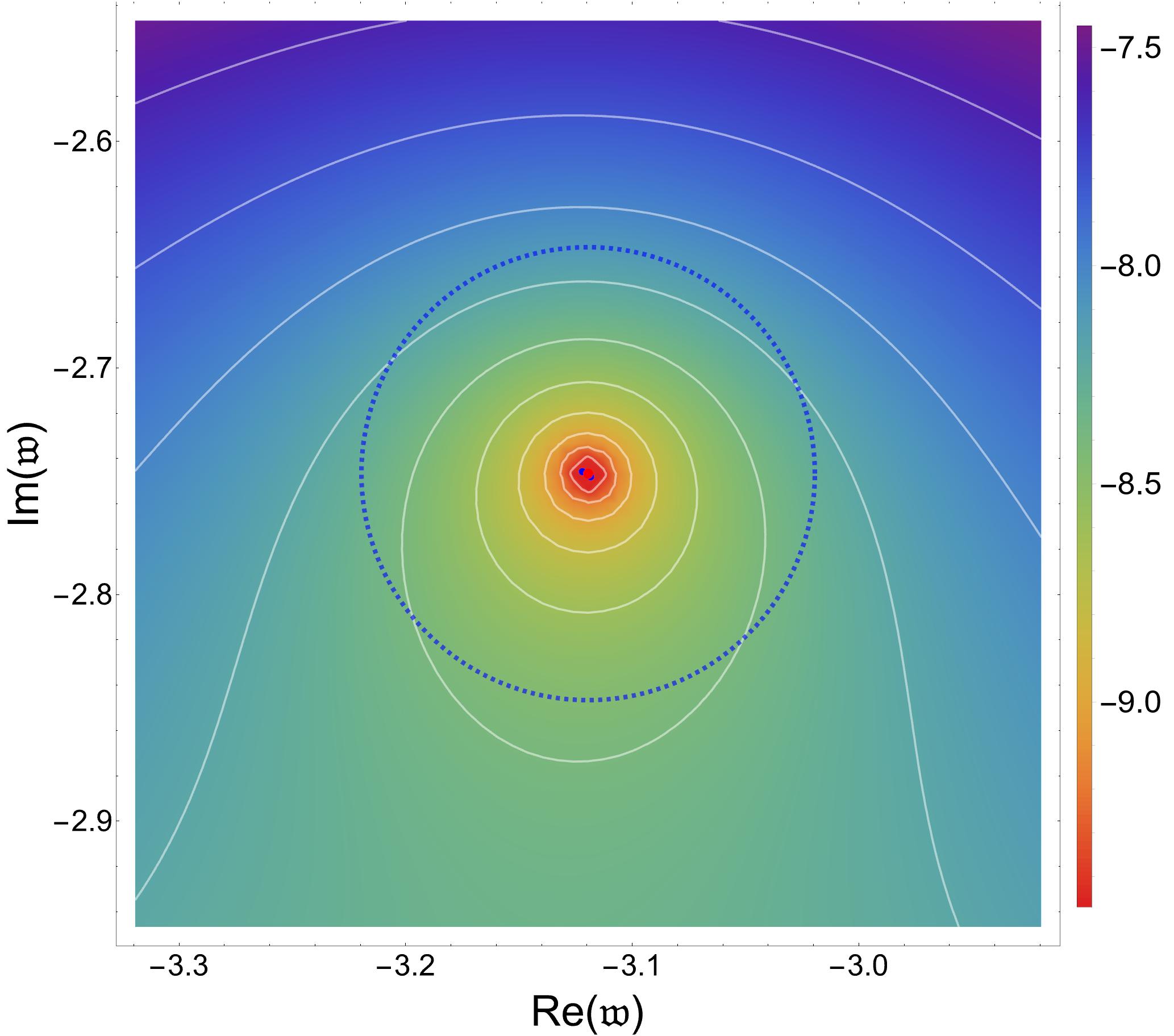
Refer to caption
(a) m2l2=0superscript𝑚2superscript𝑙20m^{2}l^{2}=0, 𝔮=0𝔮0\mathfrak{q}=0.
Refer to caption
(b) m2l2=0superscript𝑚2superscript𝑙20m^{2}l^{2}=0, 𝔮=10𝔮10\mathfrak{q}=10.
Refer to caption
(c) m2l2=3superscript𝑚2superscript𝑙23m^{2}l^{2}=-3, 𝔮=0𝔮0\mathfrak{q}=0.
Refer to caption
(d) m2l2=3superscript𝑚2superscript𝑙23m^{2}l^{2}=-3, 𝔮=10𝔮10\mathfrak{q}=10.
Figure 16: Close-up of the scalar pseudospectrum in the L2superscript𝐿2L^{2}-norm around the first QNF for different values of 𝔮𝔮\mathfrak{q} and m2l2superscript𝑚2superscript𝑙2m^{2}l^{2}. The red dot corresponds to the QNF, the white lines represent the boundaries of various full ε𝜀\varepsilon-pseudospectra, and the dashed blue circle symbolizes a circle with a radius of 101superscript10110^{-1} centered on the QNF. The heat map corresponds to the logarithm in base 10 of the inverse of the resolvent. Here the selective pseudospectra computed with random local potential perturbations of size 101superscript10110^{-1} is denoted by blue dots hidden behind the QNF.
Refer to caption
(a) m2l2=0superscript𝑚2superscript𝑙20m^{2}l^{2}=0, 𝔮=0𝔮0\mathfrak{q}=0.
Refer to caption
(b) m2l2=0superscript𝑚2superscript𝑙20m^{2}l^{2}=0, 𝔮=10𝔮10\mathfrak{q}=10.
Refer to caption
(c) m2l2=3superscript𝑚2superscript𝑙23m^{2}l^{2}=-3, 𝔮=0𝔮0\mathfrak{q}=0.
Refer to caption
(d) m2l2=3superscript𝑚2superscript𝑙23m^{2}l^{2}=-3, 𝔮=10𝔮10\mathfrak{q}=10.
Figure 17: Scalar pseudospectrum in the L2superscript𝐿2L^{2}-norm for different values of 𝔮𝔮\mathfrak{q} and m2l2superscript𝑚2superscript𝑙2m^{2}l^{2}. In the lower panels, we present selective and full pseudospectra. The red dots represent the QNFs, and the white lines denote the boundaries of different full ε𝜀\varepsilon-pseudospectra. The heat map corresponds to the logarithm in base 10 of the inverse of the resolvent, while the blue, cyan, green, and yellow dots indicate different selective ε𝜀\varepsilon-pseudospectra computed with random local potential perturbations of size 101superscript10110^{-1}, 103superscript10310^{-3}, 105superscript10510^{-5}, and 107superscript10710^{-7}; respectively. In the upper panels, we represent the condition numbers.

Next we move on to the transverse gauge field of section 4.2 and display the results for its pseudospectrum in the L2superscript𝐿2L^{2}-norm. In figure 18 we zoom in on the first QNF, while in figure 19 we show the pseudospectrum down to the position of the fourth QNF. We again observe open contour lines indicating instability under generic perturbations. As for the scalar field, the qualitative shape of the pseudospectra is very similar to what we found in the energy norm. However, we once again find that in the L2superscript𝐿2L^{2}-norm the spectrum is more unstable under generic perturbations and more stable under local potential perturbations. This becomes clear upon comparing the pseudospectra in figure 19 to those in figure 13 corresponding to the energy norm.
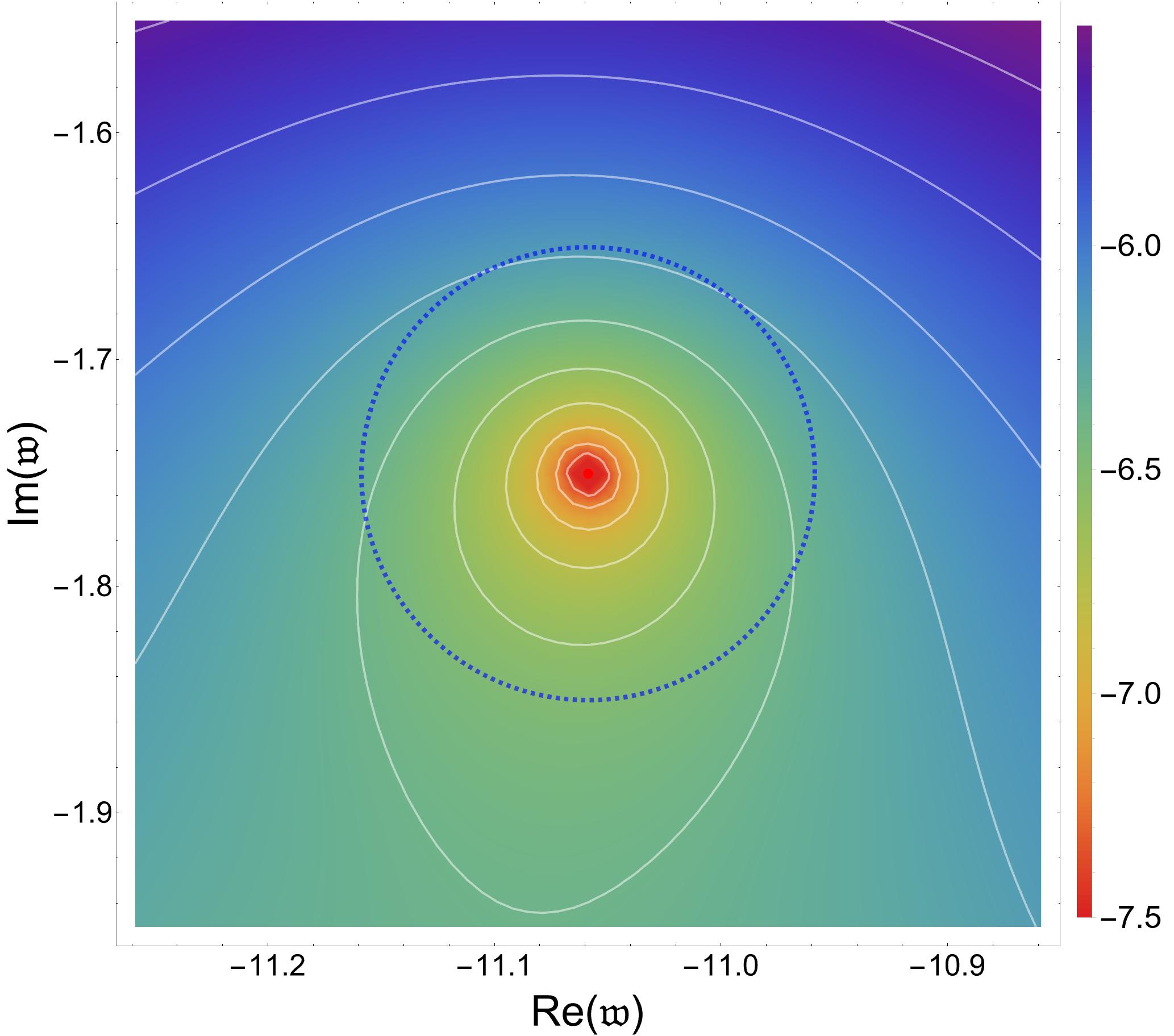
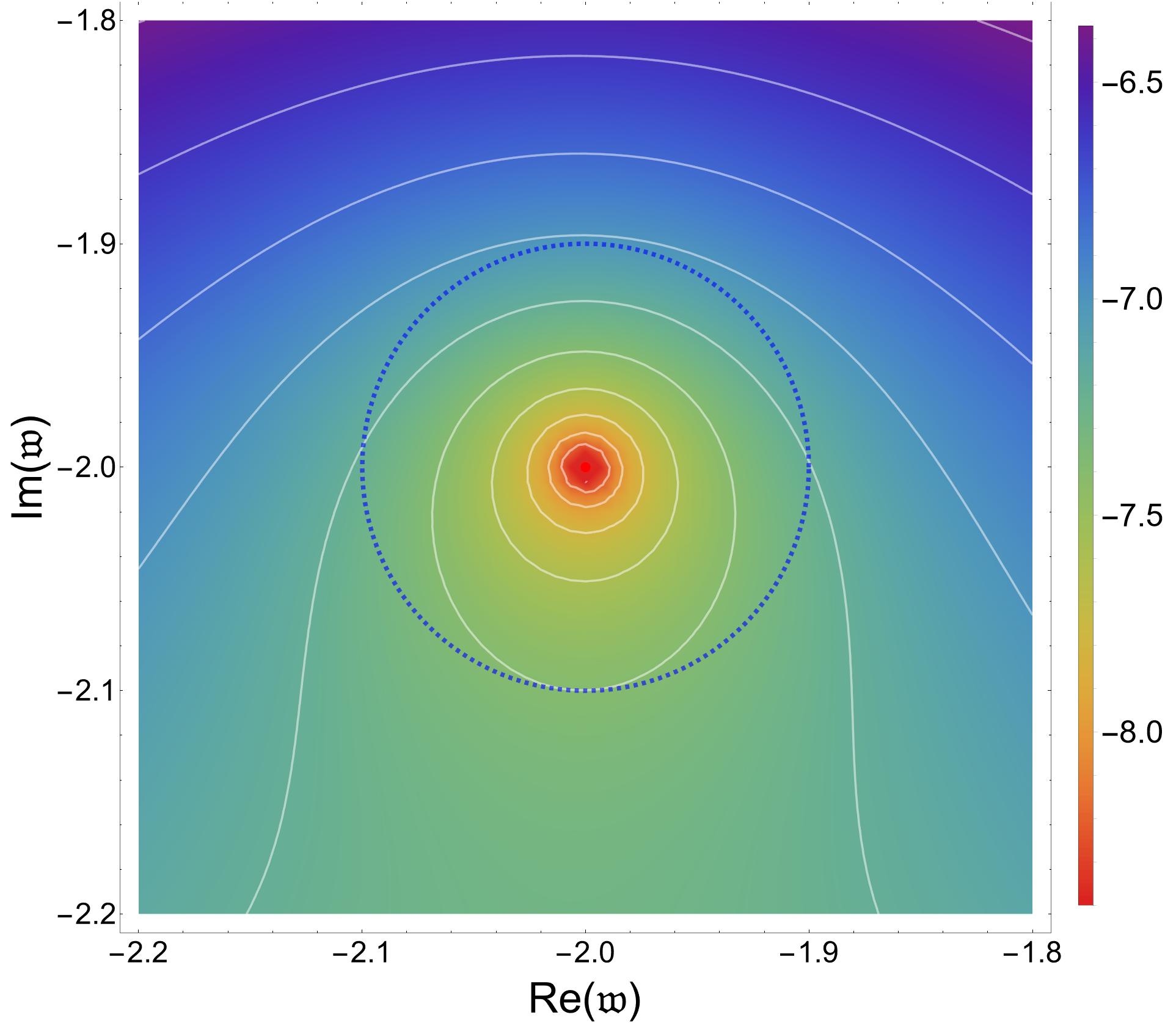
Refer to caption
(a) 𝔮=0𝔮0\mathfrak{q}=0.
Refer to caption
(b) 𝔮=10𝔮10\mathfrak{q}=10.
Figure 18: Close-up of the transverse gauge field pseudospectrum in the L2superscript𝐿2L^{2}-norm around the first QNF for different values of 𝔮𝔮\mathfrak{q}. The red dot corresponds to the QNF, the white lines represent the boundaries of various full ε𝜀\varepsilon-pseudospectra, and the dashed blue circle symbolizes a circle with a radius of 101superscript10110^{-1} centered on the QNF. The heat map corresponds to the logarithm in base 10 of the inverse of the resolvent. Here the selective pseudospectra computed with random local potential perturbations of size 101superscript10110^{-1} is hidden by the QNF.
Refer to caption
(a) 𝔮=0𝔮0\mathfrak{q}=0.
Refer to caption
(b) 𝔮=10𝔮10\mathfrak{q}=10.
Figure 19: Transverse gauge field pseudospectrum in the L2superscript𝐿2L^{2}-norm for different values of 𝔮𝔮\mathfrak{q}. In the lower panels, we present selective and full pseudospectra. The red dots represent the QNFs, and the white lines denote the boundaries of different full ε𝜀\varepsilon-pseudospectra. The heat map corresponds to the logarithm in base 10 of the inverse of the resolvent, while the blue, cyan, green, and yellow dots indicate different selective ε𝜀\varepsilon-pseudospectra computed with random local potential perturbations of size 101superscript10110^{-1}, 103superscript10310^{-3}, 105superscript10510^{-5}, and 107superscript10710^{-7}; respectively. In the upper panels, we represent the condition numbers.

We end this section by pointing out that while qualitatively similar, the pseudospectra in the energy and L2superscript𝐿2L^{2}-norm are quantitatively different. Indeed, although the shape of the contour map for the same model is very similar in both norms the quantitative value of the pseudospectrum as illustrated by the color code varies markedly from the energy to the L2superscript𝐿2L^{2}-norm. This observation further stresses the importance of properly defining a physically motivated norm: the discrepancy in the definition of size of the potential perturbations between the L2superscript𝐿2L^{2} and energy norms results in quantitatively different phenomenology.

Appendix D Numerical Values of the QNFs

In this appendix we provide the numerical values of the first 10 quasinormal frequencies for the models discussed in the main text. For purposes of presentation we limit the precision to 15 significant figures.

n𝑛n Re(𝔴n)Resubscript𝔴𝑛\mathrm{Re}(\mathfrak{w}_{n}) Im(𝔴n)Imsubscript𝔴𝑛\mathrm{Im}(\mathfrak{w}_{n})
111 ±3.11945159116590plus-or-minus3.11945159116590\pm 3.11945159116590 2.746675744340612.74667574434061-2.74667574434061
222 ±5.16952097576223plus-or-minus5.16952097576223\pm 5.16952097576223 4.763570116920464.76357011692046-4.76357011692046
333 ±7.18793082599961plus-or-minus7.18793082599961\pm 7.18793082599961 6.769564909076206.76956490907620-6.76956490907620
444 ±9.19719929048412plus-or-minus9.19719929048412\pm 9.19719929048412 8.772481103020298.77248110302029-8.77248110302029
555 ±11.2026757899702plus-or-minus11.2026757899702\pm 11.2026757899702 10.774162396509710.7741623965097-10.7741623965097
666 ±13.2062465176047plus-or-minus13.2062465176047\pm 13.2062465176047 12.775238982840412.7752389828404-12.7752389828404
777 ±15.2087360641333plus-or-minus15.2087360641333\pm 15.2087360641333 14.775979302574714.7759793025747-14.7759793025747
888 ±17.2105584199107plus-or-minus17.2105584199107\pm 17.2105584199107 16.776515358650916.7765153586509-16.7765153586509
999 ±19.2119427139029plus-or-minus19.2119427139029\pm 19.2119427139029 18.776918993919918.7769189939199-18.7769189939199
101010 ±21.2130253291193plus-or-minus21.2130253291193\pm 21.2130253291193 20.777232384586020.7772323845860-20.7772323845860
Table 1: Neutral scalar QNFs for m2l2=0superscript𝑚2superscript𝑙20m^{2}l^{2}=0 and 𝔮=0𝔮0\mathfrak{q}=0.
n𝑛n Re(𝔴n)Resubscript𝔴𝑛\mathrm{Re}(\mathfrak{w}_{n}) Im(𝔴n)Imsubscript𝔴𝑛\mathrm{Im}(\mathfrak{w}_{n})
111 ±11.0586349863470plus-or-minus11.0586349863470\pm 11.0586349863470 1.750385668264341.75038566826434-1.75038566826434
222 ±12.2041502935249plus-or-minus12.2041502935249\pm 12.2041502935249 3.498278561730633.49827856173063-3.49827856173063
333 ±13.5234927685557plus-or-minus13.5234927685557\pm 13.5234927685557 5.379969975519635.37996997551963-5.37996997551963
444 ±14.9758148001587plus-or-minus14.9758148001587\pm 14.9758148001587 7.336293053802627.33629305380262-7.33629305380262
555 ±16.5292996000810plus-or-minus16.5292996000810\pm 16.5292996000810 9.333515525954149.33351552595414-9.33351552595414
666 ±18.1599632430830plus-or-minus18.1599632430830\pm 18.1599632430830 11.352704612790711.3527046127907-11.3527046127907
777 ±19.8500241826712plus-or-minus19.8500241826712\pm 19.8500241826712 13.383251941324113.3832519413241-13.3832519413241
888 ±21.5863602228304plus-or-minus21.5863602228304\pm 21.5863602228304 15.419202070274215.4192020702742-15.4192020702742
999 ±23.3592481371511plus-or-minus23.3592481371511\pm 23.3592481371511 17.457208867977917.4572088679779-17.4572088679779
101010 ±25.1614156884878plus-or-minus25.1614156884878\pm 25.1614156884878 19.495401980353619.4954019803536-19.4954019803536
Table 2: Neutral scalar QNFs for m2l2=0superscript𝑚2superscript𝑙20m^{2}l^{2}=0 and 𝔮=10𝔮10\mathfrak{q}=10.
n𝑛n Re(𝔴n)Resubscript𝔴𝑛\mathrm{Re}(\mathfrak{w}_{n}) Im(𝔴n)Imsubscript𝔴𝑛\mathrm{Im}(\mathfrak{w}_{n})
111 ±2.19881456585250plus-or-minus2.19881456585250\pm 2.19881456585250 1.759534627133001.75953462713300-1.75953462713300
222 ±4.21189720328773plus-or-minus4.21189720328773\pm 4.21189720328773 3.774888235786663.77488823578666-3.77488823578666
333 ±6.21554314901884plus-or-minus6.21554314901884\pm 6.21554314901884 5.777257013165145.77725701316514-5.77725701316514
444 ±8.21716723825394plus-or-minus8.21716723825394\pm 8.21716723825394 7.778080219543007.77808021954300-7.77808021954300
555 ±10.2180612360290plus-or-minus10.2180612360290\pm 10.2180612360290 9.778473884006589.77847388400658-9.77847388400658
666 ±12.2186177048135plus-or-minus12.2186177048135\pm 12.2186177048135 11.778697471480811.7786974714808-11.7786974714808
777 ±14.2189931785234plus-or-minus14.2189931785234\pm 14.2189931785234 13.778838929051413.7788389290514-13.7788389290514
888 ±16.2192614139935plus-or-minus16.2192614139935\pm 16.2192614139935 15.778935284886715.7789352848867-15.7789352848867
999 ±18.2194613734973plus-or-minus18.2194613734973\pm 18.2194613734973 17.779004534316017.7790045343160-17.7790045343160
101010 ±20.2196154334378plus-or-minus20.2196154334378\pm 20.2196154334378 19.779056366930519.7790563669305-19.7790563669305
Table 3: Neutral scalar QNFs for m2l2=3superscript𝑚2superscript𝑙23m^{2}l^{2}=-3 and 𝔮=0𝔮0\mathfrak{q}=0.
n𝑛n Re(𝔴n)Resubscript𝔴𝑛\mathrm{Re}(\mathfrak{w}_{n}) Im(𝔴n)Imsubscript𝔴𝑛\mathrm{Im}(\mathfrak{w}_{n})
111 ±10.6370087422563plus-or-minus10.6370087422563\pm 10.6370087422563 1.063562414004801.06356241400480-1.06356241400480
222 ±11.6542293745917plus-or-minus11.6542293745917\pm 11.6542293745917 2.664761739798282.66476173979828-2.66476173979828
333 ±12.8816366495948plus-or-minus12.8816366495948\pm 12.8816366495948 4.468559503057454.46855950305745-4.46855950305745
444 ±14.2652641255372plus-or-minus14.2652641255372\pm 14.2652641255372 6.381404088812566.38140408881256-6.38140408881256
555 ±15.7667370212845plus-or-minus15.7667370212845\pm 15.7667370212845 8.353839817580538.35383981758053-8.35383981758053
666 ±17.3576290472434plus-or-minus17.3576290472434\pm 17.3576290472434 10.358750113784110.3587501137841-10.3587501137841
777 ±19.0169202769993plus-or-minus19.0169202769993\pm 19.0169202769993 12.381047271568612.3810472715686-12.3810472715686
888 ±20.7291315800900plus-or-minus20.7291315800900\pm 20.7291315800900 14.412265812665114.4122658126651-14.4122658126651
999 ±22.4828389281553plus-or-minus22.4828389281553\pm 22.4828389281553 16.447626656090616.4476266560906-16.4476266560906
101010 ±24.2695453187766plus-or-minus24.2695453187766\pm 24.2695453187766 18.484426107211518.4844261072115-18.4844261072115
Table 4: Neutral scalar QNFs for m2l2=3superscript𝑚2superscript𝑙23m^{2}l^{2}=-3 and 𝔮=10𝔮10\mathfrak{q}=10.
n𝑛n Re(𝔴n)Resubscript𝔴𝑛\mathrm{Re}(\mathfrak{w}_{n}) Im(𝔴n)Imsubscript𝔴𝑛\mathrm{Im}(\mathfrak{w}_{n})
111 ±2.00000000000000plus-or-minus2.00000000000000\pm 2.00000000000000 2.000000000000002.00000000000000-2.00000000000000
222 ±4.00000000000000plus-or-minus4.00000000000000\pm 4.00000000000000 4.000000000000004.00000000000000-4.00000000000000
333 ±6.00000000000000plus-or-minus6.00000000000000\pm 6.00000000000000 6.000000000000006.00000000000000-6.00000000000000
444 ±8.00000000000000plus-or-minus8.00000000000000\pm 8.00000000000000 8.000000000000008.00000000000000-8.00000000000000
555 ±10.0000000000000plus-or-minus10.0000000000000\pm 10.0000000000000 10.000000000000010.0000000000000-10.0000000000000
666 ±12.0000000000000plus-or-minus12.0000000000000\pm 12.0000000000000 12.000000000000012.0000000000000-12.0000000000000
777 ±14.0000000000000plus-or-minus14.0000000000000\pm 14.0000000000000 14.000000000000014.0000000000000-14.0000000000000
888 ±16.0000000000000plus-or-minus16.0000000000000\pm 16.0000000000000 16.000000000000016.0000000000000-16.0000000000000
999 ±18.0000000000000plus-or-minus18.0000000000000\pm 18.0000000000000 18.000000000000018.0000000000000-18.0000000000000
101010 ±20.0000000000000plus-or-minus20.0000000000000\pm 20.0000000000000 20.000000000000020.0000000000000-20.0000000000000
Table 5: Transverse gauge field QNFs for 𝔮=0𝔮0\mathfrak{q}=0.
n𝑛n Re(𝔴n)Resubscript𝔴𝑛\mathrm{Re}(\mathfrak{w}_{n}) Im(𝔴n)Imsubscript𝔴𝑛\mathrm{Im}(\mathfrak{w}_{n})
111 ±10.6311305880202plus-or-minus10.6311305880202\pm 10.6311305880202 1.074010863419591.07401086341959-1.07401086341959
222 ±11.6456703226270plus-or-minus11.6456703226270\pm 11.6456703226270 2.680580572683962.68058057268396-2.68058057268396
333 ±12.8710360299982plus-or-minus12.8710360299982\pm 12.8710360299982 4.488910909327084.48891090932708-4.48891090932708
444 ±14.2530488610374plus-or-minus14.2530488610374\pm 14.2530488610374 6.405630353115996.40563035311599-6.40563035311599
555 ±15.7531754716734plus-or-minus15.7531754716734\pm 15.7531754716734 8.381445828895878.38144582889587-8.38144582889587
666 ±17.3428934333756plus-or-minus17.3428934333756\pm 17.3428934333756 10.389355154694710.3893551546947-10.3893551546947
777 ±19.0011254785217plus-or-minus19.0011254785217\pm 19.0011254785217 12.414353642225812.4143536422258-12.4143536422258
888 ±20.7123581254599plus-or-minus20.7123581254599\pm 20.7123581254599 14.448036653819214.4480366538192-14.4480366538192
999 ±22.4651463361787plus-or-minus22.4651463361787\pm 22.4651463361787 16.485670017242516.4856700172425-16.4856700172425
101010 ±24.2509798299875plus-or-minus24.2509798299875\pm 24.2509798299875 18.524583557341718.5245835573417-18.5245835573417
Table 6: Transverse gauge field QNFs for 𝔮=10𝔮10\mathfrak{q}=10.

Appendix E Pseudospectrum Algorithm

In this appendix we give a more explicit description of the algorithm employed when computing the full pseudospectrum and condition numbers using theorem 2.7. For the sake of clarity, we do not present here the code but instead the following illustrative flowchart:

[Uncaptioned image]

References

  • (1) H.-P. Nollert, TOPICAL REVIEW: Quasinormal modes: the characteristic ‘sound’ of black holes and neutron stars, Class. Quant. Grav. 16 (1999) R159–R216.
  • (2) K. D. Kokkotas and B. G. Schmidt, Quasinormal modes of stars and black holes, Living Rev. Rel. 2 (1999) 2 [gr-qc/9909058].
  • (3) E. Berti, V. Cardoso and A. O. Starinets, Quasinormal modes of black holes and black branes, Class. Quant. Grav. 26 (2009) 163001 [0905.2975].
  • (4) N. Franchini and S. H. Völkel, Testing General Relativity with Black Hole Quasi-Normal Modes, 2305.01696.
  • (5) J. M. Maldacena, The Large N limit of superconformal field theories and supergravity, Adv. Theor. Math. Phys. 2 (1998) 231–252 [hep-th/9711200].
  • (6) O. Aharony, S. S. Gubser, J. M. Maldacena, H. Ooguri and Y. Oz, Large N field theories, string theory and gravity, Phys. Rept. 323 (2000) 183–386 [hep-th/9905111].
  • (7) M. Ammon and J. Erdmenger, Gauge/gravity duality: Foundations and applications. Cambridge University Press, Cambridge, 4, 2015.
  • (8) J. Zaanen, Y. Liu, Y. Sun and K. Schalm, Holographic Duality in Condensed Matter Physics. Cambridge University Press, 2015.
  • (9) S. A. Hartnoll, A. Lucas and S. Sachdev, Holographic Quantum Matter. MIT Press, 2018.
  • (10) G. Policastro, D. T. Son and A. O. Starinets, The Shear viscosity of strongly coupled N=4 supersymmetric Yang-Mills plasma, Phys. Rev. Lett. 87 (2001) 081601 [hep-th/0104066].
  • (11) R. Baier, P. Romatschke, D. T. Son, A. O. Starinets and M. A. Stephanov, Relativistic viscous hydrodynamics, conformal invariance, and holography, JHEP 04 (2008) 100 [0712.2451].
  • (12) S. Bhattacharyya, V. E. Hubeny, S. Minwalla and M. Rangamani, Nonlinear Fluid Dynamics from Gravity, JHEP 02 (2008) 045 [0712.2456].
  • (13) P. Kovtun, D. T. Son and A. O. Starinets, Viscosity in strongly interacting quantum field theories from black hole physics, Phys. Rev. Lett. 94 (2005) 111601 [hep-th/0405231].
  • (14) S. S. Gubser, Breaking an Abelian gauge symmetry near a black hole horizon, Phys. Rev. D 78 (2008) 065034 [0801.2977].
  • (15) S. A. Hartnoll, C. P. Herzog and G. T. Horowitz, Building a Holographic Superconductor, Phys. Rev. Lett. 101 (2008) 031601 [0803.3295].
  • (16) C. P. Herzog, P. Kovtun, S. Sachdev and D. T. Son, Quantum critical transport, duality, and M-theory, Phys. Rev. D 75 (2007) 085020 [hep-th/0701036].
  • (17) G. T. Horowitz and V. E. Hubeny, Quasinormal modes of AdS black holes and the approach to thermal equilibrium, Phys. Rev. D 62 (2000) 024027 [hep-th/9909056].
  • (18) D. Birmingham, I. Sachs and S. N. Solodukhin, Conformal field theory interpretation of black hole quasinormal modes, Phys. Rev. Lett. 88 (2002) 151301 [hep-th/0112055].
  • (19) P. K. Kovtun and A. O. Starinets, Quasinormal modes and holography, Phys. Rev. D 72 (2005) 086009 [hep-th/0506184].
  • (20) G. Policastro, D. T. Son and A. O. Starinets, From AdS / CFT correspondence to hydrodynamics, JHEP 09 (2002) 043 [hep-th/0205052].
  • (21) C. P. Herzog and S. S. Pufu, The Second Sound of SU(2), JHEP 04 (2009) 126 [0902.0409].
  • (22) I. Amado, M. Kaminski and K. Landsteiner, Hydrodynamics of Holographic Superconductors, JHEP 05 (2009) 021 [0903.2209].
  • (23) P. Kovtun, Lectures on hydrodynamic fluctuations in relativistic theories, J. Phys. A 45 (2012) 473001 [1205.5040].
  • (24) I. Amado, C. Hoyos-Badajoz, K. Landsteiner and S. Montero, Hydrodynamics and beyond in the strongly coupled N=4 plasma, JHEP 07 (2008) 133 [0805.2570].
  • (25) B. Withers, Short-lived modes from hydrodynamic dispersion relations, JHEP 06 (2018) 059 [1803.08058].
  • (26) S. Grozdanov, P. K. Kovtun, A. O. Starinets and P. Tadić, The complex life of hydrodynamic modes, Journal of High Energy Physics 2019 (nov, 2019).
  • (27) S. Grozdanov, P. K. Kovtun, A. O. Starinets and P. Tadić, Convergence of the gradient expansion in hydrodynamics, Physical Review Letters 122 (jun, 2019).
  • (28) H.-P. Nollert, About the significance of quasinormal modes of black holes, Phys. Rev. D 53 (1996) 4397–4402 [gr-qc/9602032].
  • (29) H.-P. Nollert and R. H. Price, Quantifying excitations of quasinormal mode systems, J. Math. Phys. 40 (1999) 980–1010 [gr-qc/9810074].
  • (30) J. L. Jaramillo, R. P. Macedo and L. Al Sheikh, Pseudospectrum and Black Hole Quasinormal Mode Instability, Phys. Rev. X 11 (2021), no. 3 031003 [2004.06434].
  • (31) K. Destounis, R. P. Macedo, E. Berti, V. Cardoso and J. L. Jaramillo, Pseudospectrum of Reissner-Nordström black holes: Quasinormal mode instability and universality, Phys. Rev. D 104 (2021), no. 8 084091 [2107.09673].
  • (32) S. Sarkar, M. Rahman and S. Chakraborty, Perturbing the perturbed: Stability of quasi-normal modes in presence of a positive cosmological constant, 2304.06829.
  • (33) M. H.-Y. Cheung, K. Destounis, R. P. Macedo, E. Berti and V. Cardoso, Destabilizing the Fundamental Mode of Black Holes: The Elephant and the Flea, Phys. Rev. Lett. 128 (2022), no. 11 111103 [2111.05415].
  • (34) E. Berti, V. Cardoso, M. H.-Y. Cheung, F. Di Filippo, F. Duque, P. Martens and S. Mukohyama, Stability of the fundamental quasinormal mode in time-domain observations against small perturbations, Phys. Rev. D 106 (2022), no. 8 084011 [2205.08547].
  • (35) R. A. Konoplya and A. Zhidenko, First few overtones probe the event horizon geometry, 2209.00679.
  • (36) A. Courty, K. Destounis and P. Pani, Quasinormal mode (in)stability and strong cosmic censorship, 2307.11155.
  • (37) V. Boyanov, K. Destounis, R. Panosso Macedo, V. Cardoso and J. L. Jaramillo, Pseudospectrum of horizonless compact objects: A bootstrap instability mechanism, Phys. Rev. D 107 (2023), no. 6 064012 [2209.12950].
  • (38) L. N. Trefethen and M. Embree, Spectra and Pseudospectra. Princeton University Press, Princeton, 2005.
  • (39) M. Isi, M. Giesler, W. M. Farr, M. A. Scheel and S. A. Teukolsky, Testing the no-hair theorem with GW150914, Phys. Rev. Lett. 123 (2019), no. 11 111102 [1905.00869].
  • (40) M. Giesler, M. Isi, M. A. Scheel and S. Teukolsky, Black Hole Ringdown: The Importance of Overtones, Phys. Rev. X 9 (2019), no. 4 041060 [1903.08284].
  • (41) C. D. Capano, M. Cabero, J. Westerweck, J. Abedi, S. Kastha, A. H. Nitz, Y.-F. Wang, A. B. Nielsen and B. Krishnan, Observation of a multimode quasi-normal spectrum from a perturbed black hole, 2105.05238.
  • (42) C. D. Capano, J. Abedi, S. Kastha, A. H. Nitz, J. Westerweck, Y.-F. Wang, M. Cabero, A. B. Nielsen and B. Krishnan, Statistical validation of the detection of a sub-dominant quasi-normal mode in GW190521, 2209.00640.
  • (43) P. K. Kovtun and A. O. Starinets, Quasinormal modes and holography, Physical Review D 72 (oct, 2005).
  • (44) C. M. Warnick, On quasinormal modes of asymptotically anti-de Sitter black holes, Commun. Math. Phys. 333 (2015), no. 2 959–1035 [1306.5760].
  • (45) L. N. Trefethen, Spectral Methods in MATLAB. Society for Industrial and Applied Mathematics, USA, 2000.
  • (46) J. P. Boyd, Chebyshev and Fourier spectral methods. Dover Publications Inc., 2000.
  • (47) T. Kato, Perturbation theory for linear operators, vol. 132. Springer Science & Business Media, 2013.
  • (48) D. H. Richard Courant, Methods of Mathematical Physics Volume 1. Wiley-VCH, 1 ed., 1989.
  • (49) R. A. Horn and C. R. Johnson, Matrix analysis. Cambridge University Press, second ed., 2013.
  • (50) I. R. Klebanov and E. Witten, AdS / CFT correspondence and symmetry breaking, Nucl. Phys. B 556 (1999) 89–114 [hep-th/9905104].
  • (51) P. Bizoń, T. Chmaj and P. Mach, A toy model of hyperboloidal approach to quasinormal modes, Acta Phys. Polon. B 51 (2020) 1007 [2002.01770].
  • (52) R. Panosso Macedo, Hyperboloidal approach for static spherically symmetric spacetimes: a didactical introduction and applications in black-hole physics, 2307.15735.
  • (53) E. Gasperin and J. L. Jaramillo, Energy scales and black hole pseudospectra: the structural role of the scalar product, Class. Quant. Grav. 39 (2022), no. 11 115010 [2107.12865].
  • (54) P. Breitenlohner and D. Z. Freedman, Positive Energy in anti-De Sitter Backgrounds and Gauged Extended Supergravity, Phys. Lett. B 115 (1982) 197–201.
  • (55) L. N. Trefethen, A. E. Trefethen, S. C. Reddy and T. A. Driscoll, Hydrodynamic stability without eigenvalues, Science 261 (1993), no. 5121 578–584.
  • (56) I. Amado, C. Hoyos-Badajoz, K. Landsteiner and S. Montero, Residues of correlators in the strongly coupled N=4 plasma, Phys. Rev. D 77 (2008) 065004 [0710.4458].
  • (57) S. Grozdanov, K. Schalm and V. Scopelliti, Black hole scrambling from hydrodynamics, Phys. Rev. Lett. 120 (2018), no. 23 231601 [1710.00921].
  • (58) M. Blake, H. Lee and H. Liu, A quantum hydrodynamical description for scrambling and many-body chaos, JHEP 10 (2018) 127 [1801.00010].
  • (59) M. Blake, R. A. Davison, S. Grozdanov and H. Liu, Many-body chaos and energy dynamics in holography, JHEP 10 (2018) 035 [1809.01169].
  • (60) A. Biggs and J. Maldacena, Scaling similarities and quasinormal modes of D0 black hole solutions, 2303.09974.
  • (61) J. Maldacena, A simple quantum system that describes a black hole, 2303.11534.
  • (62) J. L. Jaramillo, R. Panosso Macedo and L. A. Sheikh, Gravitational Wave Signatures of Black Hole Quasinormal Mode Instability, Phys. Rev. Lett. 128 (2022), no. 21 211102 [2105.03451].
  • (63) I. Amado, C. Hoyos-Badajoz, K. Landsteiner and S. Montero, Absorption lengths in the holographic plasma, JHEP 09 (2007) 057 [0706.2750].
  • (64) K. Landsteiner, The Sound of Strongly Coupled Field Theories: Quasinormal Modes In AdS, AIP Conf. Proc. 1458 (2012), no. 1 174–189 [1202.3550].
  • (65) L. Gavassino, M. M. Disconzi and J. Noronha, Dispersion relations alone cannot guarantee causality, 2307.05987.