Intuitionistic Fuzzy Broad Learning System: Enhancing Robustness Against Noise and Outliers

Abstract

In the realm of data classification, broad learning system (BLS) has proven to be a potent tool that utilizes a layer-by-layer feed-forward neural network. It consists of feature learning and enhancement segments, working together to extract intricate features from input data. The traditional BLS treats all samples as equally significant, which makes it less robust and less effective for real-world datasets with noises and outliers. To address this issue, we propose the fuzzy BLS (F-BLS) model, which assigns a fuzzy membership value to each training point to reduce the influence of noises and outliers. In assigning the membership value, the F-BLS model solely considers the distance from samples to the class center in the original feature space without incorporating the extent of non-belongingness to a class. We further propose a novel BLS based on intuitionistic fuzzy theory (IF-BLS). The proposed IF-BLS utilizes intuitionistic fuzzy numbers based on fuzzy membership and non-membership values to assign scores to training points in the high-dimensional feature space by using a kernel function. We evaluate the performance of proposed F-BLS and IF-BLS models on $44$ UCI benchmark datasets across diverse domains. Furthermore, Gaussian noise is added to some UCI datasets to assess the robustness of the proposed F-BLS and IFBLS models. Experimental results demonstrate superior generalization performance of the proposed F-BLS and IF-BLS models compared to baseline models, both with and without Gaussian noise. Additionally, we implement the proposed F-BLS and IF-BLS models on the Alzheimer’s Disease Neuroimaging Initiative (ADNI) dataset, and promising results showcase the model’s effectiveness in real-world applications. The proposed methods offer a promising solution to enhance the BLS framework’s ability to handle noise and outliers. It holds potential for applications in various classification problems, highlighting its versatility and practicality.

I Introduction

The structure and operations of biological neurons in the brain serve as the basis for the class of machine learning techniques known as artificial neural networks (ANNs). ANNs are composed of interconnected nodes (neurons) that use mathematical operations to process and transfer information. ANNs are designed to discover patterns and correlations in data and then utilize that knowledge to make predictions. Deep learning is one of the most prominent branches of machine learning that employs ANNs with multiple layers to perform complex tasks such as speech recognition [1], natural language processing [2], image recognition [3] and so on.

One of the prime advantages of deep learning is its capacity to automatically extract high-level features from raw data, eliminating the need for manual feature engineering. Deep learning also has the upper hand of being able to generalize effectively to new data, which allows it to make correct predictions even on data that has never been shown to it before. Apart from many advantages, there are some drawbacks of deep learning architectures. Deep learning models include several layers, millions of parameters, and an iterative learning process, making them extremely complicated. It can be computationally overloaded and time-consuming to train such models iteratively to determine a huge number of parameters. Deep learning models demand powerful hardware, such as GPUs or TPUs. A lack of such materials might stymie the training process. These disadvantages severely limit the potential uses of deep learning models beyond speech and image recognition and give space to other models to spread their wings.

Randomized neural networks (RNNs) [4, 5] are neural network that incorporates randomness in the topology and learning process of the model. This randomness allows RNNs to learn with fewer tunable parameters, in less computational time, and without the requirement of savvy hardware. Extreme learning machine (ELM) [6, 7] and random vector functional link neural network (RVFLNN) [8, 9] are two popular RNNs. In both networks, the parameters (weights and biases) of the hidden layer are randomly initialized from a suitable continuous probability distribution and stay untouched during the entire training period. Both ELM and RVFLNN uses the least-square method (provides a closed-form solution) to determine the output parameters. The direct links from the input layer to the output layer in RVFLNN significantly improve the generalization performance by functioning as a regularization tool [10]. In addition, RVFLNN provides quick training speed and universal approximation capability [11].

Recently, the broad learning system (BLS) [12] (inspired by RVFLNN), a class of flat neural networks, was proposed. BLS employs a layer-by-layer approach to extract informative features from the input data. BLS has three primary segments: a feature learning segment, an enhancement segment, and the output segment. In the feature learning and enhancement segment, the input data is transformed into a high-dimensional feature space using a set of projection mappings. These projections are produced by a collection of Gaussian matrices that are independently and identically distributed (IID) and initialized at random. As a result of the feature learning and enhancement segment, a collection of high-dimensional features is produced that effectively extract important information from the input data. To train the BLS model, only the output layer parameters need to be computed by the least-squares method. In comparison to traditional deep neural networks (DNNs), BLS has several advantages. For example, it does not need backpropagation, which might simplify the training process and lessen the likelihood of overfitting; its ability to learn from a small number of training samples; and faster training speed due to closed form solution. The universal approximation capability of BLS [13] makes it more promising among researchers. The adaptable topology of BLS makes it possible to train and update the model effectively in an incremental way [12], and when training data is scarce, BLS may have superior generalization performance than deep learning techniques [14].

The BLS has been applied in various applications. In [15], recurrent-BLS (R-BLS) and gated-BLS (G-BLS) models were developed and applied for text classification. In [16], a limited penetrable visibility graph (LPVG)-based BLS method was used for the visual evoked potential (VEP)-based Brain–computer interface (BCI) system. The graph convolutional broad network (GCB-net) and BLS were employed collaboratively in recognizing emotions through EEG signals in [17]. Using a knowledge module and a broad selective sampling module, Wang et al. [18] suggested a knowledge-augmented BLS (KABLS) that offers a multichannel selective sampling network to decouple the mixed-type pattern defects of wafer maps. In order to increase communication efficiency and lower communication costs in a communication distributed architecture, Liang et al. [19] introduced the decentralized learning communication-efficient algorithm for elastic-net BLS.

There has been a range of distinct variants of the BLS architecture proposed in the literature, each with its unique features, advantages, and limitations. The double-kernelized weighted broad learning system (DKWBLS) [20] was developed to manage the imbalanced data. Wang et al. [21] proposed a BLS-based multi-modal material identification paradigm. This technique lowers the joint feature dimensionality by optimizing the correlation between two features of the input samples with the assistance of unsupervised feature extraction. In [22], the authors proposed a time-varying iterative learning algorithm utilizing gradient descent (GD) for optimizing the parameters in the enhancement layer, feature layer, and output layer. Feng and Chen [23] proposed a hybrid system known as neuro-fuzzy BLS (NeuroFBLS). NeuroFBLS is created by combining a human-like reasoning approach based on a set of IF-THEN fuzzy rules from the fuzzy inference system with the learning and linking structure of the BLS. NeuroFBLS employs the k-means clustering technique to create fuzzy subsystems, resulting in an increase in the computational burden of the model.

BLS has a number of benefits over conventional machine learning and deep learning models [24]. However, each sample in the BLS model is given a uniform weight when creating the optimal classifier, which makes it susceptible to noise and outliers. Outliers are data points that deviate greatly from the majority of the data points, whereas noise refers to random abnormalities or oscillations in the data [25]. When noise and outliers are present in the dataset, they can skew the learning process and results in poor generalization performance of the BLS model.

Fuzzy theory is successfully employed in machine learning models [26, 27] to ameliorate the adverse effects of noise or outliers on model performance. The fuzzy theory uses the distance between the sample and the corresponding class center to generate a degree membership function. This membership scheme enables the model to deal with outliers and noise. In [28], intuitionistic fuzzy (IF) membership was presented as an advanced version of the fuzzy membership scheme. The IF theory uses the membership and non-membership functions to assign an IF score to each sample to deal with the noise and outliers efficiently. Membership and non-membership values of a sample measure the degree of belongingness and non-belongingness of that sample to a particular class.

To get motivated by the remarkable ability of fuzzy theory to handle the noise and outliers in the data, in this paper we amalgamate the fuzzy and intuitionistic fuzzy theory with the BLS model. We propose two novel models, namely fuzzy BLS (F-BLS) and intuitionistic fuzzy BLS (IF-BLS) to cope with the noisy samples and the outliers that have trespassed in the dataset. The following are the main contributions of this paper:

1. We propose a novel fuzzy broad learning system (F-BLS). The fuzzy membership assigns a different weightage to each sample based on its distance from the class center to address the issue of noise and outliers. Due to this, the sample near the class center gets a higher weightage, whereas the sample far from the class center gets a lower weightage. Therefore, it easily handles the issue of outliers present in the datasets.

2. We propose a novel intuitionistic fuzzy broad learning system (IF-BLS). By employing a kernel function, IF-BLS uses membership and non-membership functions to assign an IF number to each sample in the high-dimensional feature space. Based on the IF number, finally, a fuzzy score is assigned to each sample in the dataset. IF sets allow for a more wide representation of uncertainty than traditional fuzzy theory and can handle the noise and outliers efficiently.

3. The experiments are conducted over $44$ UCI benchmark datasets from various domains. The outcomes of the experiments demonstrate that the proposed IF-BLS has superior performance and beats the compared baseline models, and F-BLS shows a competitive nature when it comes to handling noise and outliers.

4. The proposed F-BLS and IF-BLS models are rigorously tested by adding Gaussian noise to six diverse UCI datasets for comparative analysis. The experiments, conducted under noisy conditions, provide additional evidence highlighting the significance of the proposed F-BLS and IF-BLS models as robust approaches in situations where noise and outliers pose significant challenges.

5. As an application, the proposed F-BLS and IF-BLS models are applied to detect Alzheimer’s disease. The experimental results demonstrate that the proposed F-BLS and IF-BLS models outperform the baseline models in terms of accuracy.

The remaining structure of the paper is organized as follows. In Section II, we provide a brief overview of BLS, fuzzy membership schemes, and intuitionistic fuzzy membership (IFM). In Section III, we derive the mathematical formulation of the proposed F-BLS and IF-BLS models. In Section IV, the discussion of the experimental results and statistical comparisons are made with the existing state-of-the-art models on various UCI datasets with and without Gaussian noise and on the ADNI dataset. Finally, we conclude the paper in Section V by suggesting directions for future research.

II Related Works

In this section, we go through the architecture of BLS along with its mathematical formulation, fuzzy membership schemes, and intuitionistic fuzzy membership. Let $\bigl{\{}\left(X,T\right)|\,X\in\mathbb{R}^{N\times D},\,T\in\mathbb{R}^{N\times C}\big{\}}$ be the training data where $X$ is the matrix of input samples and $T$ is the target matrix. Here, there are total $N$ training samples, each of which has dimension (no. of features) $D$ and $C$ number of classes. Let $x_{r}\in X$ and $t_{r}\in T$, then $x_{r}=\left(x_{r1},x_{r2},\ldots,x_{rD}\right)$ and $t_{r}=\left(t_{r1},t_{r2},\ldots,t_{rC}\right)$, and both are row vectors.

II-A Broad Learning System (BLS) [12]

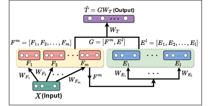
Figure 1: The architecture of the BLS model.

The architecture of the BLS is shown in Figure 1. We briefly give the mathematical formulations of BLS segment by segment.
Segment-1: Here, original input features are transformed into random feature spaces. Let there be $m$ groups and each feature group having $p$ nodes in the feature space. Then

$$F_{i}=\mathcal{F}_{i}\left(XW_{F_{i}}+\beta_{F_{i}}\right)\in\mathbb{R}^{N\times p},\leavevmode\nobreak\ \leavevmode\nobreak\ i=1,2,\ldots,m,$$ (1)

where $\mathcal{F}i$, $W_{F_{i}}\in\mathbb{R}^{D\times p}$ and $\beta_{F_{i}}\in\mathbb{R}^{N\times p}$ are feature map, randomly generated weight matrix, and bias matrix for the $i^{th}$ feature group, respectively. The augmented output of the $m$ feature groups is:

$$F^{m}=[F_{1},F_{2},\ldots,F_{m}]\in\mathbb{R}^{N\times mp}.$$ (2)

Segment-2: Augmented feature matrix $(F^{m})$ is projected to enhancement spaces via random transformations followed by the activation functions. Let $l$ be the number of enhancement groups, and each enhancement group has $q$ nodes. Then

$$E_{j}=\chi_{j}\left(F^{m}W_{E_{j}}+\beta_{E_{j}}\right)\in\mathbb{R}^{N\times q},\leavevmode\nobreak\ \leavevmode\nobreak\ j=1,2,\ldots,l.$$ (3)

Where $\chi_{j}$ is the activation function used to generate nonlinear features. $W_{E_{j}}\in\mathbb{R}^{mp\times q}$ is a randomly generated weight matrix connecting the augmented feature matrix $(F^{m})$ to $j^{th}$ enhancement group, and $\beta_{E_{j}}\in\mathbb{R}^{N\times q}$ is the bias matrix corresponding to the $j^{th}$ enhancement group. The resultant output of the $l$ enhancement groups is

$$E^{l}=[E_{1},E_{2},\ldots,E_{l}]\in\mathbb{R}^{N\times lq}.$$ (4)

Segment-3: Finally, the resultant enhancement matrix $(E^{l})$ along with the augmented feature matrix $(F^{m})$ is sent to the output layer and the final outcome is calculated as follows:

$$\hat{T}=[F^{m},E^{l}]W_{T}=GW_{T},$$ (5)

where $G=[F^{m},E^{l}]\in\mathbb{R}^{N\times(mp+lq)}$ is the concatenated matrix and $W_{T}\in\mathbb{R}^{(mp+lq)\times C}$ is the unknown weights matrix connecting the augmented feature layer and resultant enhancement layer to the output layer. The optimization problem of BLS is written as follows:

$$W_{T_{\min}}=\underset{{W_{T}}}{\text{argmin}}\,\frac{C}{2}\|GW_{T}-T\|_{2}^{2}+\frac{1}{2}\|W_{T}\|_{2}^{2},$$ (6)

where $C$ is the regularization parameter. After solving the convex quadratic problem (6), the optimal solution is given as:

$$W_{T_{\min}}=\left\{\begin{array}[]{ll}\left({G}^{t}{G}+\frac{1}{C}I\right)^{-1}{G}^{t}{T},&\text{if}\leavevmode\nobreak\ \leavevmode\nobreak\ (mp+lq)\leq N,\vspace{3mm}\\ {G}^{t}\left({G}{G}^{t}+\frac{1}{C}I\right)^{-1}{T},&\text{if}\leavevmode\nobreak\ \leavevmode\nobreak\ N<(mp+lq),\end{array}\right.$$ (7)

where $I$ is an identity matrix of appropriate dimension and $(.)^{t}$ is the transpose operator.

II-B Fuzzy Membership Scheme [29]

Let $X$ be the crisp set and $\theta:X\rightarrow[0,1]$ be the membership function which assigns fuzzy membership values to each sample $x_{r}\in X$. Define $\mathcal{A}=\bigl{\{}(x_{r},t_{r},\vartheta(x_{r}))|\,x_{r}\in\mathbb{R}^{1\times D},\,t_{r}\in\mathbb{R}^{1\times C},\,r=1,2,\ldots,N\bigl{\}}$ be the fuzzy set. The membership function for each training sample $x_{r}$ is defined as:

$$\vartheta\left(x_{r}\right)=\left\{\begin{array}[]{ll}1-\frac{\left\|x_{r}-C_{pos}\right\|}{R_{pos}+\delta},&t_{r}=+1,\\ 1-\frac{\left\|x_{r}-C_{neg}\right\|}{R_{neg}+\delta},&t_{r}=-1,\end{array}\right.$$ (8)

where $C_{pos}(C_{neg})$ and $R_{pos}(R_{neg})$ are the class center and the the radius of the positive (negative) class, respectively, and $\delta$ is a very small positive parameter. $t_{r}=+1\leavevmode\nobreak\ (-1)$ denotes the positive (negative) class sample. In the original feature space, the membership function takes into account the distance between each sample and its associated class center. The center of each class is defined as:

$$C_{pos}=\frac{1}{N_{pos}}\sum_{t_{r}=+1}x_{r}\leavevmode\nobreak\ \leavevmode\nobreak\ \text{and}\leavevmode\nobreak\ \leavevmode\nobreak\ C_{neg}=\frac{1}{N_{neg}}\sum_{t_{r}=-1}x_{r},$$ (9)

where $N_{pos}$ and $N_{neg}$ are the total number of samples in the positive and negative classes, respectively. And the radii are defined as:

$$R_{pos}=\underset{{t_{r}=+1}}{\max}\|x_{r}-C_{pos}\|\leavevmode\nobreak\ \leavevmode\nobreak\ \text{and}\leavevmode\nobreak\ \leavevmode\nobreak\ R_{neg}=\underset{{t_{r}=-1}}{\max}\|x_{r}-C_{neg}\|.$$ (10)

Finally the score matrix $\mathcal{S}$ for the dataset $X$ is defined as: $\mathcal{S}=\text{$diag$}\left(\vartheta(x_{1}),\vartheta(x_{2}),\ldots,\vartheta(x_{N})\right).$

II-C Intuitionistic Fuzzy Membership (IFM) Scheme [28]

While the fuzzy set was introduced by Zadeh [30] in 1965, whereas the intuitionistic fuzzy set (IFS) was proposed by Atanassov and Atanassov [31] to cope with uncertainty difficulties, and it allows for a precise simulation of the situation using current information and observations [28]. Here, the IFM scheme for the crisp set $X$ at the kernel space is discussed by projecting the dataset $X$ onto a high-dimensional space. An IFS is defined as: $\widetilde{\mathcal{A}}=\bigl{\{}(x_{r},t_{r},\theta(x_{r}),\widetilde{\theta}(x_{r})|\,x_{r}\in\mathbb{R}^{1\times D},\,t_{r}\in\mathbb{R}^{1\times C},\,r=1,2,\ldots,N\bigl{\}},$ where $\theta(x_{r})$ and $\widetilde{\theta}(x_{r})$ are the membership and non-membership values of the sample $x_{r}$.

• The membership mapping: The membership function $\theta:X\rightarrow[0,1]$ is defined as:

  $$\theta\left(x_{r}\right)=\left\{\begin{array}[]{ll}1-\frac{\left\|\psi(x_{r})-C_{pos}\right\|}{R_{pos}+\delta},&t_{r}=+1,\\ 1-\frac{\left\|\psi(x_{r})-C_{neg}\right\|}{R_{neg}+\delta},&t_{r}=-1,\end{array}\right.$$ (11)

  where $\psi$ is the feature (projection) mapping, $C_{pos},\leavevmode\nobreak\ C_{neg},\leavevmode\nobreak\ R_{pos},\leavevmode\nobreak\ R_{neg}$ are defined in the same way as mentioned in Subsection II-B, however, while computing these centers and radii, $\psi(x_{r})$ is taken into account instead of $x_{r}$.

• The non-membership mapping: In the IFM scheme, each training sample $x_{r}$ is additionally allocated a non-membership value (degree) that represents the ratio of heterogeneous data points to all data points in its vicinity. The non-membership function $\widetilde{\theta}:X\rightarrow[0,1]$ is defined as: $\widetilde{\theta}(x_{r})=\big{(}1-\theta(x_{r})\big{)}\Theta(x_{r}),$ where $0\leq\theta(x_{r})+\widetilde{\theta}(x_{r})\leq 1$ and $\Theta$ is calculated as follows:

  $$\Theta(x_{r})=\frac{|\{x_{l}:\|\psi(x_{r})-\psi(x_{l})\|\leq\epsilon,\leavevmode\nobreak\ y_{r}\neq y_{l}\}|}{|\{x_{l}:\|\psi(x_{r})-\psi(x_{l})\|\leq\epsilon\}|},$$ (12)

  where $\epsilon$ is the adjustable parameter used to create a neighborhood and $|.|$ represents the cardinality of a set.

• The score mapping: After calculating the membership and non-membership values (degree) of each sample, an intuitionistic fuzzy score (IFS) function is defined as follows:

  $$\Theta^{\star}(x_{r})=\left\{\begin{array}[]{lll}{\theta(x_{r})},&{\widetilde{\theta}(x_{r})=0},\\ 0,&\theta(x_{r})\leq\widetilde{\theta}(x_{r}),\\ \frac{1-\widetilde{\theta}(x_{r})}{2-\theta(x_{r})-\widetilde{\theta}(x_{r})},&\text{otherwise}.\end{array}\right.$$ (13)

• The score matrix: Finally, the score matrix $\mathcal{S}$ for the dataset $X$ is defined as: $\mathcal{S}=\text{$diag$}\left(\Theta^{\star}(x_{1}),\Theta^{\star}(x_{2}),\ldots,\Theta^{\star}(x_{N})\right).$

The membership and non-membership values are calculated in the kernel space based on the Euclidean norm (the usual inner product). As a result, the kernel technique is explored in Section 1 of the Supplementary Material.

III Proposed Fuzzy Broad Learning System (F-BLS) and Intuitionistic Fuzzy Broad Learning System (IF-BLS)

In traditional machine learning models, including BLS, each data sample is given the same weight irrespective of its nature. Naturally, a dataset is never pure, $i.e.,$ the involvement of noise and outliers in a dataset is a normal phenomenon. Although the occurrence of these noises and outliers is natural, it has a detrimental impact on the traditional BLS. Therefore, to deal with noisy samples and outliers present in the dataset, we propose two models, which are as follows:

1. Fuzzy BLS (F-BLS) by employing the membership scheme discussed in the subsection II-B.

2. Intuitionistic fuzzy BLS (IF-BLS) using the IF scheme discussed in II-C.

The fuzzy membership value in the proposed F-BLS and IF-BLS models is based on how close a sample is to the class center in the original feature space and high-dimensional feature space, respectively. These fuzzy membership values represent the degree to which a sample belongs to a certain class. The fuzzy non-membership value in the proposed IF-BLS is determined by considering the neighborhood information of the sample, expressing the extent of non-belongingness to a particular class.

The optimization problem of the proposed F-BLS and IF-BLS models are defined as follows:

$$W_{T_{\min}}=\underset{{W_{T}}}{\text{argmin}}\,\frac{C}{2}\|\mathcal{S}\zeta\|_{2}^{2}+\frac{1}{2}\|W_{T}\|_{2}^{2},$$

$$\text{s.t.}\leavevmode\nobreak\ \leavevmode\nobreak\ GW_{T}-T=\zeta,$$ (14)

where $\mathcal{S}$ denotes the score matrix. For F-BLS, the score matrix is obtained from the Subsection II-B, whereas for IF-BLS, $\mathcal{S}$ is taken from the Subsection II-C. Here, $\zeta$ refers to the error matrix. Equivalently, the formulation (III) can be written as:

$$W_{T_{\min}}=\underset{{W_{T}}}{\text{argmin}}\,\frac{C}{2}\|\mathcal{S}(GW_{T}-T)\|_{2}^{2}+\frac{1}{2}\|W_{T}\|_{2}^{2}.$$ (15)

Problem (15) is the convex quadratic programming problem (QPP) and hence possesses a unique solution. The Lagrangian of (III) is written as:

$$\mathcal{L}(W_{T},\zeta,\lambda)=\frac{C}{2}\|\mathcal{S}\zeta\|_{2}^{2}+\frac{1}{2}\|W_{T}\|_{2}^{2}-\lambda^{t}(GW_{T}-T-\zeta),$$ (16)

where $\lambda$ is the Lagrangian multiplier and $(.)^{t}$ is the transpose operator. Differentiating $\mathcal{L}$ partially w.r.t. each parameters, $i.e.,W_{T},\zeta\leavevmode\nobreak\ \text{and}\leavevmode\nobreak\ \lambda$; and equating them to zero, we obtain

$$\frac{\partial\mathcal{L}}{\partial W_{T}}=0\Rightarrow W_{T}-G^{t}\lambda=0\Rightarrow W_{T}=G^{t}\lambda,$$ (17)

$$\frac{\partial\mathcal{L}}{\partial\zeta}=0\Rightarrow C\mathcal{S}^{t}(\mathcal{S}\zeta)+\lambda=0\Rightarrow\lambda=-C\mathcal{S}^{t}\mathcal{S}\zeta,$$ (18)

$$\frac{\partial\mathcal{L}}{\partial\lambda}=0\Rightarrow GW_{T}-T-\zeta=0\Rightarrow\zeta=GW_{T}-T.$$ (19)

Substituting Eq. (19) in (18), we get

$$\lambda=-C\mathcal{S}^{t}\mathcal{S}(GW_{T}-T).$$ (20)

On substituting the value of $\lambda$ obtained in Eq. (20) in (17), we obtain

$$W_{T}=G^{t}(-C\mathcal{S}^{t}\mathcal{S}(GW_{T}-T)).$$ (21)

After simplifying Eq. (21), we get

$$W_{T}=\left(G^{t}\mathcal{S}^{2}G+\frac{1}{C}I\right)^{-1}G^{t}\mathcal{S}^{2}T,$$ (22)

where $I$ is the identity matrix of the appropriate dimension. On substituting the values of Eq. (17) and (18) in (19), we obtain

$$\lambda=\left(\frac{1}{C}\left(\mathcal{S}^{t}\mathcal{S}\right)^{-1}+GG^{t}\right)^{-1}T.$$ (23)

Putting the value of $\lambda$ obtained in Eq. (23) in (17), we get

$$W_{T}=G^{t}\left(\frac{1}{C}\left(\mathcal{S}^{t}\mathcal{S}\right)^{-1}+GG^{t}\right)^{-1}T.$$ (24)

Since $\mathcal{S}$ is the diagonal matrix; therefore it is symmetric, i.e., $\mathcal{S}^{t}=\mathcal{S}$. Therefore, Eq. (24) can be rewritten as:

$$W_{T}=G^{t}\left(\frac{1}{C}I+\mathcal{S}^{2}GG^{t}\right)^{-1}\mathcal{S}^{2}T.$$ (25)

We get two distinct formulas, (22) and (25), that can be utilized to determine $W_{T}$. It is worth noting that both formulas involve the calculation of the matrix inverse. However, if the number of features ($mp+lq$) in $G$ is less than the number of samples ($N$), we employ the formula derived in equation (22) to compute $W_{T}$. Conversely, when the number of samples ($N$) is fewer than the number of features ($mp+lq$) in $G$, we opt for the formula derived in equation (25) to calculate $W_{T}$. As a result, we possess the advantage of calculating the matrix inverse either in the feature or sample space, contingent upon the specific scenario. Therefore, the optimal solution of (III) is given as follows:

$$W_{T}=\left\{\begin{array}[]{ll}{\left(G^{t}\mathcal{S}^{2}G+\frac{1}{C}I\right)^{-1}G^{t}\mathcal{S}^{2}T},&\text{if}\leavevmode\nobreak\ \leavevmode\nobreak\ (mp+lq)\leq N,\vspace{3mm}\\ {G^{t}\left(\frac{1}{C}I+\mathcal{S}^{2}GG^{t}\right)^{-1}\mathcal{S}^{2}T},&\text{if}\leavevmode\nobreak\ \leavevmode\nobreak\ N<(mp+lq).\end{array}\right.$$ (26)

Table I: The classification accuracies, standard deviations and the corresponding best hyperparameters of the proposed F-BLS and IF-BLS models along with the existing baseline models, i.e., BLS, ELM, and NeuroFBLS on UCI datasets.

Model	BLS [12]	ELM [6]	NeuroFBLS [23]	F-BLS (Proposed)	IF-BLS (Proposed)
Dataset	Acc. $\pm$ Std.	Acc. $\pm$ Std.	Acc. $\pm$ Std.	Acc. $\pm$ Std.	Acc. $\pm$ Std.
	($C,p,m,q$)	($C,h_{l}$)	($C,N_{fn},N_{fg},q$)	($C,p,m,q$)	($C,\mu,p,m,q$)
acute_inflammation	$\textbf{100.0000}\pm 0.0000$	$\textbf{100.0000}\pm 0.0000$	$\textbf{100.0000}\pm 0.0000$	$\textbf{100.0000}\pm 0.0000$	$\textbf{100.0000}\pm 0.0000$
	($0,5,9,45$)	($0.000001,15$)	($0.000001,5,3,5$)	($0.000001,5,5,35$)	($100,0.03125,5,3,85$)
acute_nephritis	$\textbf{100.0000}\pm 0.0000$	$\textbf{100.0000}\pm 0.0000$	$\textbf{100.0000}\pm 0.0000$	$\textbf{100.0000}\pm 0.0000$	$\textbf{100.0000}\pm 0.0000$
	($1,5,5,35$)	($1,45$)	($0.000001,5,1,45$)	($1,5,3,105$)	($10000,0.03125,15,9,35$)
bank	$89.7366\pm 0.6268$	$89.4051\pm 0.5757$	$89.5817\pm 0.7048$	$\textbf{89.7590}\pm 0.6556$	$89.4051\pm 0.6945$
	($1000000,25,21,85$)	($10000,195$)	($0.000001,15,15,45$)	($1000000,15,15,65$)	($1000000,0.5,45,19,15$)
blood	$77.0389\pm 13.5212$	$77.1732\pm 13.4210$	$76.9056\pm 13.2215$	$75.7002\pm 11.4520$	$\textbf{77.4398}\pm 13.2299$
	($1,15,15,65$)	($0.0001,15$)	($0.0001,5,7,5$)	($100,15,7,65$)	($10000,0.125,20,5,15$)
breast_cancer	$69.8851\pm 24.9547$	$66.6727\pm 34.1162$	$70.1754\pm 44.6249$	$72.2868\pm 27.5906$	$\textbf{83.1579}\pm 26.8828$
	($0,15,3,105$)	($0.000001,15$)	($100,5,1,5$)	($0.000001,40,1,55$)	($1000000,8,5,3,75$)
breast_cancer_wisc	$88.4183\pm 3.9756$	$87.9897\pm 7.7412$	$\textbf{90.7081}\pm 5.2416$	$88.2775\pm 5.6270$	$88.9938\pm 5.3499$
	($1,25,15,85$)	($1,155$)	($1,30,17,55$)	($1,35,13,75$)	($1000000,1,20,21,85$)
breast_cancer_wisc_diag	$\textbf{93.8503}\pm 3.6668$	$92.0882\pm 2.4964$	$89.2750\pm 5.1813$	$93.6749\pm 3.3596$	$93.4964\pm 1.7150$
	($1,40,5,65$)	($0.01,195$)	($0.000001,5,17,5$)	($10000,40,3,5$)	($1000000,0.125,50,17,75$)
breast_cancer_wisc_prog	$79.8462\pm 6.2766$	$79.8077\pm 4.6243$	$79.8590\pm 8.7734$	$78.3077\pm 3.6281$	$\textbf{79.8718}\pm 6.2766$
	($100,15,1,85$)	($0.01,205$)	($1,5,19,55$)	($100,25,1,105$)	($10000,4,30,1,75$)
chess_krvkp	$84.3862\pm 2.4087$	$72.0312\pm 8.7903$	$70.4004\pm 3.6413$	$84.2921\pm 2.6204$	$\textbf{84.9184}\pm 2.4254$
	($0.01,20,3,45$)	($10000,165$)	($0.000001,40,21,15$)	($0.01,40,5,15$)	($1000000,0.03125,30,3,75$)
congressional_voting	$63.6782\pm 3.6889$	$62.7586\pm 2.0880$	$\textbf{63.9080}\pm 3.7774$	$60.2299\pm 5.7815$	$59.5402\pm 4.2544$
	($100,50,7,55$)	($0.01,25$)	($0.01,5,3,25$)	($1,30,9,85$)	($1000000,1,25,21,35$)
conn_bench_sonar_mines_rocks	$69.2451\pm 13.9054$	$60.5807\pm 5.6916$	$60.6272\pm 10.5182$	$69.1521\pm 11.3172$	$\textbf{80.2091}\pm 13.5518$
	($0.01,5,3,95$)	($10000,165$)	($0.0001,10,17,5$)	($0.0001,10,1,95$)	($1,16,50,15,105$)
credit_approval	$87.5362\pm 11.1132$	$85.3623\pm 10.5060$	$84.4928\pm 10.5832$	$86.3768\pm 11.1250$	$\textbf{88.5507}\pm 10.3423$
	($0.01,15,1,5$)	($10000,45$)	($1,5,21,15$)	($0.01,5,15,65$)	($100,4,10,1,85$)
cylinder_bands	$69.9258\pm 3.4408$	$66.2193\pm 3.6640$	$69.5336\pm 6.8956$	$69.1338\pm 3.2817$	$\textbf{72.8536}\pm 1.5525$
	($1,25,1,85$)	($0.01,125$)	($0.01,15,13,95$)	($1,50,13,85$)	($100,4,5,19,65$)
echocardiogram	$83.9316\pm 7.4670$	$83.9031\pm 5.8108$	$80.9402\pm 3.6463$	$84.6724\pm 7.2724$	$\textbf{88.4900}\pm 6.1265$
	($1000000,20,1,15$)	($0.01,155$)	($1,15,3,105$)	($100,10,1,105$)	($1000000,8,50,19,5$)
fertility	$90.0000\pm 10.0000$	$89.0000\pm 9.6177$	$\textbf{92.0000}\pm 6.7082$	$91.0000\pm 8.2158$	$91.0000\pm 8.2158$
	($100,10,1,75$)	($0.000001,55$)	($1,10,9,35$)	($100,45,1,85$)	($1000000,1,40,17,85$)
haberman_survival	$70.2750\pm 7.3768$	$73.4902\pm 8.4751$	$73.4902\pm 8.4751$	$69.6563\pm 10.0681$	$\textbf{75.4574}\pm 8.5088$
	($1,25,21,95$)	($0.000001,5$)	($1,5,1,5$)	($1000000,45,3,5$)	($1000000,16,35,1,75$)
heart_hungarian	$77.5804\pm 9.7137$	$73.4717\pm 10.8177$	$70.3565\pm 16.3687$	$78.9421\pm 9.5844$	$\textbf{83.3255}\pm 12.5494$
	($0.0001,40,1,35$)	($0.0001,75$)	($0.000001,10,1,15$)	($0.0001,5,5,25$)	($1000000,8,35,15,35$)
hepatitis	$85.1613\pm 9.8374$	$83.2258\pm 9.5148$	$\textbf{87.7419}\pm 5.7705$	$84.5161\pm 9.5148$	$\textbf{87.7419}\pm 4.2059$
	($100,5,3,75$)	($0.01,135$)	($0.0001,45,17,55$)	($1,40,19,35$)	($10000,8,30,5,75$)
hill_valley	$\textbf{82.0185}\pm 6.8334$	$77.9706\pm 2.3404$	$78.9583\pm 4.4314$	$81.6002\pm 3.4346$	$79.6249\pm 4.2790$
	($0.01,35,9,5$)	($0.01,205$)	($1,45,21,25$)	($1,25,19,75$)	($1,32,50,5,55$)
horse_colic	$86.1422\pm 4.9082$	$84.7908\pm 2.5627$	$83.9726\pm 2.9113$	$86.1385\pm 6.0478$	$\textbf{86.6938}\pm 2.5582$
	($1,35,1,55$)	($0.01,175$)	($1,5,19,95$)	($1,35,7,85$)	($1000000,2,50,17,15$)
ilpd_indian_liver	$72.0469\pm 5.2564$	$71.5296\pm 4.9025$	$72.3799\pm 5.7510$	$69.4769\pm 4.2284$	$\textbf{72.3843}\pm 6.3894$
	($100,40,1,5$)	($0.0001,15$)	($1,30,1,35$)	($100,5,1,75$)	($1000000,2,25,5,85$)
ionosphere	$88.3541\pm 9.5467$	$86.6318\pm 8.3565$	$\textbf{91.4648}\pm 3.1341$	$88.3501\pm 8.7867$	$89.1871\pm 6.4747$
	($0.01,25,19,75$)	($0.01,155$)	($1,5,21,5$)	($1,30,19,15$)	($100,2,40,17,95$)
mammographic	$78.6712\pm 2.4859$	$79.0889\pm 4.0207$	$79.5040\pm 5.5859$	$78.6744\pm 4.8822$	$\textbf{79.8192}\pm 5.3901$
	($10000,10,21,45$)	($1000000,75$)	($1,15,13,15$)	($10000,30,1,105$)	($1000000,0.25,10,19,85$)
molec_biol_promoter	$83.9394\pm 4.3409$	$68.9610\pm 6.4639$	$65.1515\pm 8.2564$	$84.9351\pm 3.7913$	$\textbf{88.7879}\pm 9.5415$
	($0.01,15,15,105$)	($0.01,205$)	($0.0001,25,3,45$)	($1,20,9,5$)	($100,8,30,7,15$)
monks_1	$75.3314\pm 11.7835$	$83.2497\pm 8.4301$	$\textbf{86.1277}\pm 10.7869$	$77.1396\pm 7.6452$	$77.6705\pm 9.3321$
	($1000000,10,1,95$)	($100,205$)	($1,50,9,75$)	($1000000,10,1,95$)	($1000000,0.5,45,19,85$)
monks_2	$73.7011\pm 4.7864$	$81.5165\pm 6.5196$	$\textbf{86.3375}\pm 8.4765$	$73.1997\pm 5.1045$	$76.1928\pm 8.1462$
	($1000000,40,19,45$)	($10000,195$)	($0.01,40,13,95$)	($1000000,45,19,105$)	($1000000,1,45,21,35$)
monks_3	$88.6241\pm 5.3273$	$90.0753\pm 3.5945$	$\textbf{91.1581}\pm 4.2862$	$87.3612\pm 2.3232$	$83.7396\pm 7.7034$
	($1000000,30,1,105$)	($1,205$)	($1,20,21,85$)	($1000000,50,1,95$)	($1000000,0.5,20,21,55$)
musk_1	$75.8311\pm 11.8581$	$67.8640\pm 4.8493$	$67.8487\pm 8.7957$	$76.6754\pm 7.2500$	$\textbf{78.9846}\pm 7.7547$
	($0.01,10,3,25$)	($0.0001,205$)	($0.01,35,21,5$)	($0.01,30,13,5$)	($10000,16,10,17,65$)
oocytes_merluccius_nucleus_4d	$\textbf{82.7776}\pm 2.5626$	$79.8407\pm 2.8977$	$80.1420\pm 3.7426$	$81.8011\pm 1.5154$	$80.9201\pm 2.2095$
	($1,35,19,55$)	($0.01,175$)	($0.0001,5,21,45$)	($1,30,21,65$)	($1000000,0.0625,40,21,55$)
oocytes_trisopterus_nucleus_2f	$\textbf{78.9371}\pm 4.6837$	$76.4211\pm 3.9279$	$75.9911\pm 2.6206$	$78.6123\pm 3.7965$	$75.9899\pm 2.3332$
	($1000000,30,1,25$)	($0.01,205$)	($0.0001,5,19,15$)	($100,40,1,75$)	($1000000,0.5,45,19,45$)
ozone	$97.1610\pm 2.2599$	$97.1217\pm 2.2639$	$\textbf{97.2401}\pm 2.1733$	$97.2006\pm 2.3139$	$97.1612\pm 2.2937$
	($1,50,17,15$)	($0.000001,5$)	($1,50,21,95$)	($100,25,1,65$)	($1,32,35,1,85$)
parkinsons	$82.5641\pm 16.4583$	$77.9487\pm 17.9121$	$\textbf{82.5641}\pm 14.8851$	$80.0000\pm 15.7437$	$82.0513\pm 9.0655$
	($100,10,3,35$)	($0.01,15$)	($0.01,10,1,25$)	($100,40,3,85$)	($1000000,4,20,15,95$)
pima	$72.0058\pm 2.8966$	$71.4888\pm 2.2956$	$72.7918\pm 4.2047$	$71.4846\pm 3.8226$	$\textbf{73.3079}\pm 1.5777$
	($100,30,1,25$)	($1000000,105$)	($0.01,5,9,65$)	($100,20,1,5$)	($1000000,1,10,9,95$)
pittsburg_bridges_T_OR_D	$89.1905\pm 5.4205$	$88.1429\pm 11.5696$	$90.1429\pm 7.9461$	$88.1905\pm 8.3581$	$\textbf{90.2381}\pm 5.9856$
	($1,30,21,65$)	($0.0001,15$)	($1,40,1,75$)	($100,30,3,15$)	($10000,2,40,5,95$)
planning	$71.9369\pm 9.2169$	$71.3814\pm 8.8534$	$72.4925\pm 9.5262$	$71.4114\pm 9.5837$	$\textbf{74.2342}\pm 8.8350$
	($100,5,1,75$)	($0.000001,5$)	($0.0001,10,1,105$)	($100,5,1,45$)	($10000,2,10,5,35$)
spambase	$89.0021\pm 4.0884$	$87.1125\pm 5.5405$	$83.2657\pm 7.5672$	$89.4582\pm 2.8438$	$\textbf{90.7407}\pm 2.4424$
	($0.01,30,19,65$)	($100,175$)	($0.000001,5,19,75$)	($0.01,10,9,55$)	($1,16,45,19,15$)
spect	$69.4340\pm 8.3745$	$67.9245\pm 3.5299$	$67.9245\pm 6.9325$	$69.4340\pm 2.7986$	$\textbf{72.4528}\pm 7.3802$
	($0.01,5,13,55$)	($0.000001,85$)	($0.01,45,11,55$)	($1,35,5,95$)	($100,16,25,9,25$)
spectf	$79.3431\pm 20.8936$	$79.3431\pm 20.8936$	$\textbf{80.8456}\pm 18.9032$	$78.9727\pm 20.4475$	$79.7345\pm 14.6711$
	($100,5,1,105$)	($0.0001,5$)	($0.01,10,1,65$)	($100,5,1,105$)	($1000000,16,30,1,75$)
statlog_australian_credit	$68.2609\pm 1.4851$	$68.1159\pm 1.1458$	$\textbf{69.2754}\pm 3.1420$	$67.8261\pm 1.5026$	$67.9710\pm 1.8757$
	($10000,35,1,5$)	($100,15$)	($1,5,17,5$)	($100,5,1,95$)	($1000000,4,10,1,45$)
statlog_german_credit	$\textbf{76.8000}\pm 2.0187$	$75.9000\pm 2.4341$	$75.8000\pm 2.8196$	$76.4000\pm 3.9115$	$76.1000\pm 2.6786$
	($1,25,1,85$)	($0.0001,105$)	($0.0001,5,19,15$)	($1000000,45,1,15$)	($1000000,0.5,50,15,95$)
statlog_heart	$82.2222\pm 2.1114$	$80.0000\pm 3.5621$	$80.7407\pm 1.0143$	$82.2222\pm 2.8085$	$\textbf{84.0741}\pm 4.8290$
	($1,30,9,105$)	($0.01,55$)	($1,40,15,105$)	($1,50,7,105$)	($10000,4,25,17,55$)
tic_tac_toe	$\textbf{98.4315}\pm 1.2836$	$86.0068\pm 7.9105$	$82.7623\pm 13.1336$	$97.8081\pm 1.7038$	$97.0768\pm 0.8768$
	($1,15,21,105$)	($10000,205$)	($0.01,35,15,95$)	($1,15,21,45$)	($10000,2,10,21,55$)
titanic	$77.9168\pm 15.5828$	$77.9168\pm 15.5828$	$78.0537\pm 13.6955$	$77.9168\pm 15.5828$	$\textbf{79.0532}\pm 15.0381$
	($10000,10,3,65$)	($0.000001,75$)	($100,5,1,55$)	($0.000001,5,1,5$)	($1,2,15,1,65$)
vertebral_column_2clases	$78.7097\pm 14.6677$	$71.2903\pm 27.1668$	$74.1935\pm 17.8516$	$76.1290\pm 19.7342$	$\textbf{83.2258}\pm 9.0236$
	($0.01,5,1,5$)	($0.000001,105$)	($0.0001,20,1,75$)	($0.01,5,3,15$)	($0.01,0.5,5,1,65$)
Avg. Acc. $\pm$ Avg. Std.	$81.3602\pm 7.116$	$79.3367\pm 7.4427$	$79.9347\pm 7.8797$	$81.009\pm 6.8422$	$\textbf{82.7697}\pm 6.4674$
Here, Avg., Acc. and Std. are used as abbreviations for average, accuracy and standard deviation, respectively.
The boldface in each row denotes the performance of the best model corresponding to the datasets.

IV Experiments and Results Analysis

To test the efficiency of proposed models, i.e., F-BLS and IF-BLS, we compare them to baseline models on publicly available UCI [32] datasets from diverse domains with and without Gaussian noise. Moreover, we implement the proposed models on the Alzheimer’s disease (AD) dataset, available on the Alzheimer’s Disease Neuroimaging Initiative (ADNI) ($adni.loni.usc.edu$).

IV-A Setup for Experiments

The experimental procedures are executed on a computing system possessing MATLAB R2023a software, an 11th Gen Intel(R) Core(TM) i7-11700 processor operating at 2.50GHz with 16.0 GB RAM, and a Windows-11 operating platform. The Gaussian kernel function is employed to project the input samples into a higher-dimensional space. The Gaussian kernel is defined as: $K(x_{1},x_{2})=exp(-\frac{\norm{x_{1}-x_{2}}^{2}}{\mu^{2}})$, where $\mu$ is the kernel parameter and we tune the $\mu$ in the range $\{2^{-5},2^{-4},\cdots,2^{5}\}$. We use the 5-fold cross-validation technique and grid search to fine-tune the hyperparameters of models. This involved splitting the dataset into five distinct, non-overlapping subsets or “folds”. In each iteration, one subset is set aside for testing while the remaining four are utilized for training. For each set of hyperparameters, we calculated the testing accuracy on each fold separately. We then determined the average testing accuracy for each set by taking the mean of these five accuracies. The highest average testing accuracy is selected as the testing accuracy of the models. Each model’s regularization parameters are selected from the set: $C=\{10^{-6},10^{-4},\cdots,10^{4},10^{6}\}$. For BLS, F-BLS, and IF-BLS, the number of feature groups is chosen from the range $m=1:2:21$; the number of feature nodes in each feature group is chosen from the range $p=5:5:50$. For NeuroFBLS, the number of fuzzy groups is chosen from the range $N_{fg}=1:2:21$; and the number of fuzzy nodes in each fuzzy group is chosen from the range $N_{fn}=5:5:50$. The number of enhancement nodes for BLS, NeuroFBLS, F-BLS, and IF-BLS is chosen from the range $q=5:5:50$ by taking the number of enhancement groups equal to $1$. For ELM, the number of hidden nodes is chosen from the range $h_{l}=5:10:205$.

IV-B Evaluation on UCI Dataset

We use 44 benchmark datasets from the UCI repository [32], spanning diverse domains, to demonstrate the efficacy of the proposed models in mitigating the challenges posed by noise and outliers. Our study involves a comparative analysis among the proposed F-BLS and IF-BLS models and the compared baseline models, namely ELM [6], BLS [12] and NeuroFBLS [23].

The performance of these models is assessed using accuracy measurements and is presented in Table I. Additionally, Table I includes the standard deviation values and the corresponding optimal hyperparameters. The average accuracies for the existing models are as follows: BLS with an average accuracy of $81.3602\%$, ELM with $79.3367\%$, and NeuroFBLS with $79.9347\%$. On the other hand, the proposed IF-BLS and F-BLS models achieved accuracies of $82.7697\%$ and $81.009\%$, respectively. In terms of average accuracy, the proposed IF-BLS secured the first position, while the proposed F-BLS ranked third. A notable finding is that the proposed IF-BLS and F-BLS models showed the most minimal standard deviation values among the compared models, with $6.4674$ and $6.8422$, respectively. This shows that the proposed IF-BLS and F-BLS models possess a high degree of certainty in their predictions.

Average accuracy can be a misleading indicator since a model’s superior performance on one dataset may make up for a model’s inferior performance on another. To mitigate the limitations of average accuracies and to determine the significance of the results, we utilized a set of statistical tests recommended by Demšar [33]. These tests are specifically designed for comparing classifiers across multiple datasets, particularly when the conditions necessary for parametric tests are not met. We employed the following tests: ranking test, Friedman test, Nemenyi post hoc test and win-tie loss sign test. By incorporating statistical tests, we aim to assess the performance of the models comprehensively and enable us to draw broad and unbiased conclusions about the models’ effectiveness. In the ranking scheme, each model is ranked based on its performance on individual datasets to evaluate its performances. Higher ranks are assigned to the worst-performing models and lower ranks to the best-performing models. By adopting this methodology, the potential compensatory effect of superior performance on one dataset offsetting inferior performance on others is considered. Suppose $\mathscr{D}$ models are being evaluated using $\mathscr{K}$ datasets, and the $d^{th}$ model’s rank on the $k^{th}$ dataset is denoted by $\mathcal{r}(d,k)$. The $d^{th}$ model’s average rank is determined as follows: $\mathcal{r}(d,*)=\left(\sum_{k=1}^{\mathscr{K}}\mathcal{r}(d,k)\right)/\mathscr{K}$. The average ranks of the models are presented in Table II. The proposed IF-BLS model achieved an average rank of $2.0341$, the lowest among all the models. Since a lower rank indicates a better-performing model, the proposed IF-BLS model emerged as the best-performing model. The Friedman test [34] compares the average ranks of models and determines whether the models have significant differences based on their rankings. The Friedman test is a nonparametric statistical test used to compare the performance of multiple models across different datasets. The models’ average rank is equal under the null hypothesis, assuming they perform equally. The Friedman test follows the chi-squared distribution ($\chi^{2}_{F}$) with $\mathscr{D}-1$ degrees of freedom (d.o.f.) $\chi^{2}_{F}=\frac{12\mathscr{K}}{\mathscr{D}(\mathscr{D}+1)}\left(\sum_{d=1}^{\mathscr{D}}\left(\mathcal{r}(d,*)\right)^{2}-\frac{\mathscr{D}(\mathscr{D}+1)^{2}}{4}\right).$ Iman and Davenport [35] demonstrated that Friedman’s $\chi^{2}_{F}$ statistic could be excessively conservative, and they proposed an alternative $F_{F}$ statistic that yields better results: $F_{F}=\chi_{F}^{2}\left(\frac{(\mathscr{K}-1)}{\mathscr{K}(\mathscr{D}-1)-\chi_{F}^{2}}\right),$ where the distribution of $F_{F}$ has $(\mathscr{D}-1)$ and $(\mathscr{K}-1)(\mathscr{D}-1)$ d.o.f.. For $\mathscr{D}=5$ and $\mathscr{K}=44$, we get $\chi^{2}_{F}=36.7596$ and $F_{F}=11.352$. According to the statistical $F-$distribution table, $F_{F}(4,172)=2.4242$ at $5\%$ level of significance. The null hypothesis is rejected since $11.352>2.4242$. As a result, the models differ significantly. Since the null hypothesis is rejected, we use the Nemenyi post hoc test [33]. Under this test, we can determine that the performance of the proposed model is significantly distinct from existing models if the average ranks differ by at least the critical difference ($C.D.$). The $C.D.$ is defined as: $C.D.=q_{\alpha}\left(\sqrt{\frac{\mathscr{D}(\mathscr{D}+1)}{6\mathscr{K}}}\right),$ where $q_{\alpha}$ is the critical value for the two-tailed Nemenyi test from the precalculated distribution table in [33]. After calculation, we get $C.D.=0.9196$ at $5\%$ level of significance ($i.e.$ at $\alpha=0.05$). As per the average ranks and average accuracy, the proposed IF-BLS emerged as the best-performing model; therefore, we make Table II $w.r.t.$ the best-performing proposed IF-BLS model. Table II presents whether there is a significant difference between the best-performing IF-BLS model and the other models or not. The average rank difference between the proposed IF-BLS is greater than the ranks of the NeuroFBLS, F-BLS, and ELM models. Thus, according to Nemenyi post hoc test, the proposed IF-BLS model differs statistically from NeuroFBLS, F-BLS, and ELM models. Therefore, the proposed IF-BLS has superior performance than the compared models. It is important to note that the proposed IF-BLS does not show the statistical difference with the BLS; however, the proposed IF-BLS model outperformed the BLS model in almost all datasets (refer to Tables I and II for accuracies and average ranks). Also, F-BLS shows a significant difference from the ELM model. Considering all these findings, we can conclude that the proposed F-BLS shows a competitive nature, and the proposed IF-BLS model is superior to the existing BLS, ELM, BLS, and NeuroFBLS models.

In addition, to analyze the models, we use pairwise win-tie-loss sign test. The “win-tie-loss” test is a prominent statistical test in research and data analysis for determining if there is a statistical difference between the outcomes of two or more models. Under the null hypothesis, which assumes that the models perform equally, each model is expected to win on half ($\mathscr{K}/2$) of the datasets out of the total number of datasets ($\mathscr{K}$). For two models to be deemed significantly distinct, it is required that each model achieves a minimum of $\mathscr{K}/2+1.96\sqrt{\mathscr{K}}/2$ victories. In the case of a tie, the score is evenly divided among the models being compared. This criterion ensures that the models’ performances are sufficiently separated to establish a statistically significant difference.

For $\mathscr{K}=44$, the threshold for determining statistical difference according to the win-tie-loss test is equal to $\mathscr{K}/2+1.96\sqrt{\mathscr{K}}/2=44/2+1.96\sqrt{44}/2=28.5006$. The pairwise win-tie-loss of models are noted in Table III. If either of the two models achieves victories in a minimum of $29$ datasets, it establishes a clear statistical distinction between them. Upon careful examination of Table III, we observe that the proposed IF-BLS model wins over the BLS, ELM, and F-BLS models by securing a number of victories: $31$, $35$, and $31$, respectively, out of a total of $44$ datasets. Thereby substantiating the superiority of the proposed IF-BLS model over its existing ELM, BLS, NeuroFBLS, and proposed F-BLS counterparts. However, IF-BLS narrowly misses achieving a statistically significant distinction from the NeuroFBLS model by just a single victory, standing at the precipice of the threshold of $29$ datasets. With a noteworthy performance, the IF-BLS model secures victories in $28$ out of $44$ datasets. Nevertheless, the winning percentage of the IF-BLS model indicates its effectiveness compared to the NeuroFBLS model. This outcome reinforces the notion that the IF-BLS model possesses notable advantages and stands as a compelling choice in terms of its overall effectiveness.

An intriguing finding emerges from comparing the traditional BLS and the proposed F-BLS models. Surprisingly, the traditional BLS outperforms the proposed F-BLS model, suggesting a plausible explanation. The F-BLS model, while assigning fuzzy values to each datapoint, solely considers membership values without incorporating the measure of the extent of non-belongingness to a class. This crucial omission indicates that only relying on fuzzy membership adversely affects the ability of the traditional BLS model to handle noise and outliers effectively. However, the remarkable performance of the IF-BLS model offers a compelling solution. By considering both membership and non-membership values when calculating the degree of fuzzy values, the IF-BLS model demonstrates its indispensability in effectively addressing the challenges posed by noise and outliers. This emphasizes how important it is to take into account both membership and non-membership values in order to combat the impact of noise and outliers.

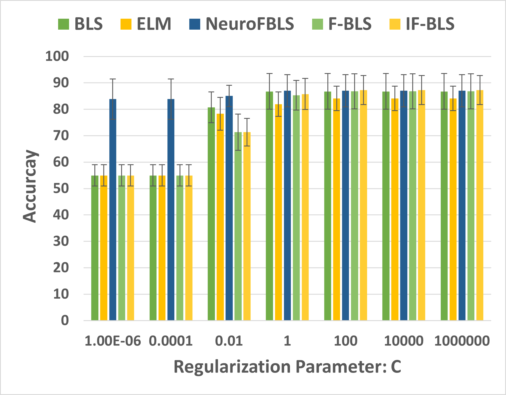
(a)

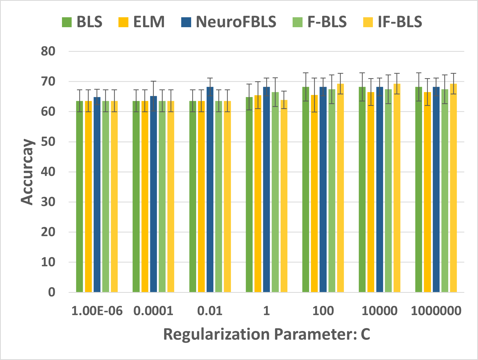
(b)

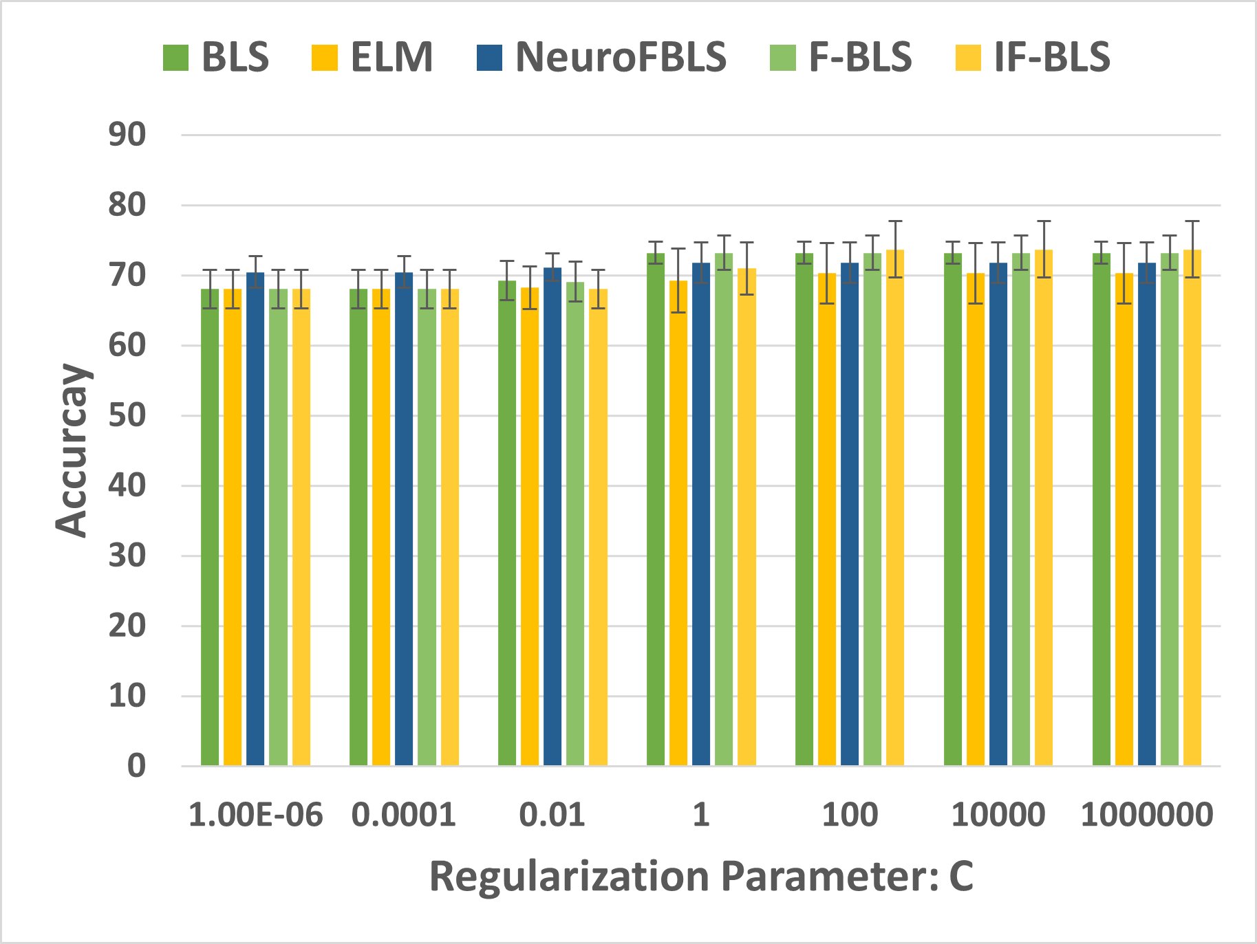
(c)

Figure 2: Accuracy along with the standard deviation (shown in thin lines on the top) of each model with respect to regularization parameter $C$ on ADNI dataset.

Table II: Differences in the rankings of the IF-BLS model against other models on UCI datasets.

Model Name	Average Rank	Rank Difference	Significant Difference (As per Nemnyi post hoc test)
IF-BLS (Proposed)	2.0341	-	N/A
BLS [12]	2.7045	0.6704	✗
NeuroFBLS [23]	3	0.9659	✓
F-BLS (Proposed)	3.2614	1.2273	✓
ELM [6]	4	1.9659	✓

Table III: Pairwise win-tie-loss of proposed and existing models on UCI datasets.

	BLS [12]	ELM [6]	NeuroFBLS [23]	F-BLS (Proposed)
ELM [6]	[$6,4,34$]
NeuroFBLS [23]	[$20,3,21$]	[$27,4,13$]
F-BLS (Proposed)	[$11,5,28$]	[$29,3,12$]	[$20,2,22$]
IF-BLS (Proposed)	[$31,2,11$]	[$35,3,6$]	[$28,3,13$]	[$31,3,10$]

IV-C Evaluation on UCI Datasets with Gaussian Noise

Table IV: The classification accuracies, standard deviations, ranks and the corresponding best parameters of the proposed F-BLS and IF-BLS models along with the existing models, i.e., BLS, ELM, and NeuroFBLS on UCI dataset with varying levels of $5\%$, $10\%$, $15\%$, and $20\%$ Gaussian noise.

Model		BLS [12]	ELM [6]	NeuroFBLS [23]	F-BLS (Proposed)	IF-BLS (Proposed)
Dataset	Noise Percentage	Acc. $\pm$ Std., Rank	Acc. $\pm$ Std., Rank	Acc. $\pm$ Std., Rank	Acc. $\pm$ Std., Rank	Acc. $\pm$ Std., Rank
		($C,p,m,q$)	($C,h_{l}$)	($C,N_{fn},N_{fg},q$)	($C,p,m,q$)	($C,\mu,p,m,q$)
breast_cancer	$5$	$70.2359\pm 26.0578$, $3$	$69.4737\pm 43.5886$, $5$	$70.1754\pm 44.6249$, $4$	$71.2704\pm 27.9532$, $2$	$\textbf{82.8070}\pm 23.9395$, $1$
		($0.0001,10,3,105$)	($0.000001,5$)	($100,5,1,5$)	($0.0001,10,1,95$)	($100,16,5,1,25$)
	$10$	$71.9722\pm 27.5470$, $3$	$67.0175\pm 45.6714$, $5$	$70.1754\pm 44.6249$, $4$	$72.6558\pm 27.6671$, $2$	$\textbf{82.4622}\pm 24.5976$, $1$
		($0,40,1,25$)	($0.000001,5$)	($100,5,1,5$)	($0.000001,25,1,15$)	($1000000,8,10,1,5$)
	$15$	$70.8832\pm 27.0047$, $3$	$66.6667\pm 44.3655$, $5$	$70.5263\pm 43.9368$, $4$	$72.3351\pm 24.3874$, $2$	$\textbf{86.6667}\pm 21.4006$, $1$
		($0,25,1,35$)	($0.0001,5$)	($100,20,1,25$)	($0.0001,5,3,105$)	($1000000,4,5,3,85$)
	$20$	$71.9419\pm 26.8794$, $2$	$67.3926\pm 42.3351$, $5$	$70.5263\pm 44.4418$, $4$	$70.5384\pm 29.7448$, $3$	$\textbf{81.7604}\pm 23.9190$, $1$
		($0,15,1,65$)	($0.0001,5$)	($100,35,17,35$)	($0.0001,15,3,5$)	($10000,4,15,3,45$)
conn_bench_sonar_mines_rocks	$5$	$68.7340\pm 9.8007$, $2$	$57.7003\pm 3.9134$, $5$	$61.5447\pm 7.7724$, $4$	$68.6527\pm 9.4446$, $3$	$\textbf{78.4204}\pm 8.9616$, $1$
		($0.01,10,1,95$)	($100,115$)	($0.0001,15,13,75$)	($0.01,35,3,35$)	($1000000,32,50,1,105$)
	$10$	$67.2009\pm 14.8713$, $2$	$57.2474\pm 12.8776$, $5$	$59.0825\pm 10.5432$, $4$	$66.8293\pm 7.7664$, $3$	$\textbf{78.2695}\pm 13.8660$, $1$
		($0.01,5,9,95$)	($1000000,145$)	($0.000001,10,17,95$)	($10000,40,9,15$)	($100,16,35,11,5$)
	$15$	$67.3171\pm 6.3730$, $3$	$67.3403\pm 7.4754$, $2$	$58.2346\pm 13.0538$, $5$	$65.8653\pm 6.4177$, $4$	$\textbf{77.8513}\pm 8.7652$, $1$
		($0.01,5,3,55$)	($10000,155$)	($0.0001,20,11,95$)	($0.0001,50,1,45$)	($1,32,5,19,15$)
	$20$	$67.7352\pm 12.7508$, $3$	$60.5923\pm 5.4069$, $5$	$61.0221\pm 20.5560$, $4$	$68.2695\pm 8.8397$, $2$	$\textbf{75.4704}\pm 15.2157$, $1$
		($0.01,5,17,95$)	($10000,75$)	($0.0001,15,11,25$)	($10000,35,21,15$)	($10000,32,50,1,55$)
hill_valley	$5$	$81.4359\pm 0.4903$, $3$	$79.0416\pm 2.3907$, $5$	$79.7840\pm 3.1142$, $4$	$\textbf{82.3433}\pm 0.7357$, $1$	$81.9311\pm 3.3660$, $2$
		($0.01,20,17,55$)	($0.01,175$)	($0.000001,10,17,85$)	($1,35,9,85$)	($1000000,0.0625,25,21,75$)
	$10$	$\textbf{80.9417}\pm 2.3794$, $1$	$76.4847\pm 3.7976$, $5$	$78.1356\pm 0.4881$, $4$	$79.4603\pm 3.1585$, $3$	$80.7758\pm 2.0920$, $2$
		($0.01,50,19,55$)	($0.01,205$)	($1,15,19,15$)	($0.01,25,17,75$)	($1000000,0.03125,20,19,25$)
	$15$	$80.2809\pm 1.9610$, $2$	$75.5790\pm 2.4486$, $5$	$76.7354\pm 2.9256$, $4$	$79.3725\pm 1.9428$, $3$	$\textbf{80.3639}\pm 1.9166$, $1$
		($0.01,30,19,25$)	($0.01,205$)	($1,35,17,95$)	($0.01,30,11,105$)	($1000000,0.03125,50,19,95$)
	$20$	$79.2089\pm 2.4190$, $3$	$74.3370\pm 2.1926$, $5$	$76.4837\pm 3.0069$, $4$	$79.4538\pm 2.4648$, $2$	$\textbf{80.0337}\pm 2.2579$, $1$
		($0.01,45,19,95$)	($0.01,195$)	($1,35,21,45$)	($0.01,40,21,55$)	($1000000,0.03125,20,15,25$)
pittsburg_bridges_T_OR_D	$5$	$89.1905\pm 9.5855$, $3$	$86.1429\pm 13.9488$, $5$	$89.2381\pm 9.5615$, $2$	$88.1429\pm 8.4472$, $4$	$\textbf{93.1429}\pm 4.4237$, $1$
		($100,40,1,55$)	($0.000001,5$)	($1,30,5,55$)	($100,15,3,105$)	($100,32,20,1,85$)
	$10$	$88.1905\pm 8.3581$, $4$	$87.2857\pm 10.0785$, $5$	$90.1429\pm 7.9461$, $2$	$88.2381\pm 6.4957$, $3$	$\textbf{92.1429}\pm 5.6944$, $1$
		($1000000,45,1,25$)	($1,115$)	($1,50,1,15$)	($100,30,9,85$)	($100,32,40,3,85$)
	$15$	$88.2381\pm 8.9271$, $2$	$86.1905\pm 11.9712$, $5$	$87.2381\pm 8.3734$, $3$	$87.1905\pm 4.5094$, $4$	$\textbf{92.1429}\pm 4.4639$, $1$
		($100,5,3,65$)	($1000000,35$)	($0.01,15,1,5$)	($100,20,3,45$)	($10000,2,45,11,15$)
	$20$	$87.2381\pm 7.4357$, $4$	$86.1429\pm 13.9488$, $5$	$92.1429\pm 5.6944$, $2$	$90.1429\pm 9.2637$, $3$	$\textbf{92.1905}\pm 5.5185$, $1$
		($100,45,1,25$)	($0.000001,5$)	($1,40,7,15$)	($10000,30,21,45$)	($10000,2,30,5,105$)
statlog_german_credit	$5$	$\textbf{77.0000}\pm 2.8940$, $1$	$76.4000\pm 2.4850$, $3$	$75.4000\pm 1.7103$, $5$	$76.9000\pm 2.5100$, $2$	$76.0000\pm 1.8708$, $4$
		($10000,25,1,35$)	($0.0001,195$)	($0.01,5,19,75$)	($100,45,1,25$)	($1000000,0.0625,50,21,15$)
	$10$	$\textbf{76.6000}\pm 3.0290$, $1$	$75.3000\pm 4.0866$, $5$	$75.8000\pm 2.4135$, $3.5$	$76.3000\pm 2.5642$, $2$	$75.8000\pm 4.1923$, $3.5$
		($1,40,1,45$)	($0.0001,165$)	($1,5,21,35$)	($1,40,1,85$)	($1000000,0.0625,45,21,105$)
	$15$	$\textbf{76.5000}\pm 1.6583$, $1.5$	$75.4000\pm 1.7819$, $4$	$74.9000\pm 2.3292$, $5$	$76.2000\pm 2.3875$, $3$	$\textbf{76.5000}\pm 1.6956$, $1.5$
		($1,20,1,65$)	($0.0001,185$)	($1,5,19,45$)	($1,45,1,105$)	($1000000,0.25,35,21,95$)
	$20$	$76.2000\pm 3.8177$, $2.5$	$75.7000\pm 1.9558$, $4$	$74.5000\pm 2.5495$, $5$	$\textbf{76.9000}\pm 1.7819$, $1$	$76.2000\pm 2.4135$, $2.5$
		($10000,40,1,15$)	($10000,105$)	($0.01,5,19,45$)	($1,25,15,5$)	($1000000,0.125,50,19,105$)
tic_tac_toe	$5$	$\textbf{97.7018}\pm 2.4968$, $1$	$81.9181\pm 20.0315$, $5$	$83.3922\pm 9.7246$, $4$	$97.2840\pm 2.1695$, $3$	$97.3882\pm 1.6115$, $2$
		($1,10,21,105$)	($1,175$)	($0.000001,15,19,25$)	($100,10,19,75$)	($1000000,1,30,21,105$)
	$10$	$\textbf{97.3893}\pm 2.0868$, $1$	$83.5951\pm 11.8785$, $4$	$80.8901\pm 10.5162$, $5$	$97.3887\pm 1.1720$, $2$	$97.2846\pm 1.6671$, $3$
		($1,15,21,105$)	($1000000,185$)	($0.000001,15,19,35$)	($100,35,19,105$)	($1000000,1,40,21,105$)
	$15$	$96.0318\pm 2.3264$, $2$	$82.4689\pm 9.2264$, $4$	$78.9998\pm 13.3383$, $5$	$95.9271\pm 3.0788$, $3$	$\textbf{96.4480}\pm 1.5491$, $1$
		($1,25,21,95$)	($100,195$)	($0.01,25,13,65$)	($1,25,21,85$)	($1000000,1,25,21,75$)
	$20$	$94.6755\pm 2.0997$, $2$	$79.2174\pm 14.1505$, $4$	$76.8161\pm 14.1961$, $5$	$93.9431\pm 3.3620$, $3$	$\textbf{95.8246}\pm 1.9521$, $1$
		($1,25,21,105$)	($1,185$)	($0.000001,20,15,55$)	($100,10,19,75$)	($1000000,1,10,21,75$)
Avg. Acc. $\pm$ Avg. Std., Avg. Rank		$80.1185\pm 8.8854$, $2.29$	$74.7764\pm 13.8336$, $4.58$	$75.4953\pm 13.6434$, $3.98$	$80.0668\pm 8.2610$, $2.63$	$\textbf{84.4949}\pm 7.8063$, $1.52$
Here, Avg., Acc. and Std. are used as abbreviations for average, accuracy and standard deviation, respectively. The boldface in each row denotes the performance of the best model corresponding to the datasets.

While the UCI datasets utilized in our study reflect real-world scenarios, it is worth noting that the presence of impurities or noise in collected data can increase for various reasons. In such circumstances, it becomes imperative to develop a robust model capable of effectively handling such challenging scenarios. To demonstrate the superiority of the proposed IF-BLS model even in adverse situations, we intentionally introduced Gaussian noise to selected UCI datasets. We have chosen $6$ diverse UCI datasets for our comparative analysis. These datasets include breast_cancer, conn_bench_sonar_mines_rocks, hill_valley, pittsburg_bridges_T_OR_D, statlog_german_credit, and tic_tac_toe, each representing a different domain. In order to ensure fairness in evaluating the models, we have selected $3$ datasets where the best-performing proposed IF-BLS model does not achieve the highest performance at the noise level of $0\%$ (indicating a loss for the proposed IF-BLS model) as per Table I. Additionally, we have chosen $3$ datasets where the proposed IF-BLS model outperforms other models at the $0\%$ noise level (indicating a win for the proposed IF-BLS model). For detailed information about the selected datasets, please refer to Table 1 of Supplementary Material. To conduct a comprehensive analysis, we introduced Gaussian noise with varying levels of $5\%$, $10\%$, $15\%$, and $20\%$ to corrupt the features of these datasets.

Comparative analysis: The accuracy and the ranks of all the models in the chosen datasets with $5\%$, $10\%$, $15\%$, and $20\%$ noise are presented in Table IV.

1. The proposed model, IF-BLS, consistently achieved the top position in the conn_bench_sonar_mines_rocks, pittsburg_bridges_T_OR_D, and breast_cancer, even without any noise. Remarkably, it maintained its superior performance even when noise is introduced. In the breast_cancer dataset, the IF-BLS model demonstrated a minimum accuracy of $81.7604\%$ at $20\%$ noise, whereas the accuracy of the second-best performing model, BLS, dropped to $71.9419\%$ at the same noise level. This comparison highlights the effectiveness of the IF-BLS model, as even its lowest accuracy remains approximately $10\%$ higher than the next best alternative, i.e., BLS. Similar results are observed in the conn_bench_sonar_mines_rocks and pittsburg_bridges_T_OR_D datasets.

2. In Table IV, we observe interesting patterns in the datasets hill_valley, statlog_german_credit, and tic_tac_toe. Initially, the proposed F-BLS and IF-BLS models did not secure the top positions at 0% noise. However, as the level of Gaussian noise increased, these models began to outperform the existing baselines. For instance, in the tic_tac_toe dataset, the proposed models initially struggled to secure top positions at $0\%$, $5\%$, and $10\%$ noise levels. However, at $15\%$ and $20\%$ noise, the proposed IF-BLS model emerged as the first-place winner. Similarly, in the hill_valley dataset, the proposed F-BLS model achieved the top rank at $5\%$ noise, while the proposed IF-BLS model secured the second rank. At $15\%$ and $20\%$ noise, the proposed IF-BLS model outperformed all baselines and the proposed F-BLS model. Furthermore, in the statlog_german_credit dataset, although the proposed models did not initially secure the first position at $0\%$, $5\%$, and $10\%$ noise levels, IF-BLS and F-BLS demonstrated their robustness by claiming the first positions at $15\%$ and $20\%$ noise, respectively.

3. The proposed IF-BLS and F-BLS models have achieved better results compared to the baseline models, securing the first and third positions in terms of average accuracy with values of $84.4949\%$ and $80.0668\%$, respectively. Furthermore, these models demonstrate superior robustness, as evidenced by their low standard deviations of $7.8063$ and $8.2610$, respectively. The combination of high average accuracy and low standard deviation indicates that the proposed IF-BLS and F-BLS models are less sensitive to noise and exhibit robust performance in handling varying conditions.

4. The proposed IF-BLS model stands out with the lowest rank of $1.52$ among all the models, and the proposed F-BLS model has a rank $2.63$. In comparison, the ELM model lags behind with a rank of $4.58$. This stark contrast in rankings demonstrates the superior performance and effectiveness of the proposed IF-BLS and F-BLS model over the existing baseline model.

By subjecting the model to challenging conditions, we aim to showcase the proposed F-BLS and IF-BLS models’ superior performance and ability to outshine other models in unfavorable scenarios. The above observations highlight the significance of the proposed F-BLS and IF-BLS models as robust models with better interpretability. They can adeptly navigate and excel in scenarios where noise and impurities pose significant challenges.

IV-D Evaluation on ADNI Dataset

Table V: The classification accuracies of the proposed F-BLS and IF-BLS models along with the existing models, i.e., BLS, ELM, RVFL and NeuroFBLS on ADNI dataset.

Model	BLS [12]	ELM [6]	NeuroFBLS [23]	F-BLS (Proposed)	IF-BLS (Proposed)
Case	Acc. $\pm$ Std.	Acc. $\pm$ Std.	Acc. $\pm$ Std.	Acc. $\pm$ Std.	Acc. $\pm$ Std.
	($C,p,m,q$)	($C,h_{l}$)	($C,N_{fn},N_{fg},q$)	($C,p,m,q$)	($C,\mu,p,m,q$)
CN_VS_AD	88.4337$\pm$6.9525	86.747$\pm$5.0401	88.6747$\pm$5.8157	88.6387$\pm$2.9016	88.8137$\pm$5.224
	(1,30,11,35)	(100,95)	(0.01,10,9,85)	(10000,35,3,55)	(100,2,15,19,95)
CN_VS_MCI	70.7695$\pm$3.093	69.0108$\pm$6.3513	70.4495$\pm$3.0157	70.2883$\pm$4.9702	71.0844$\pm$4.0305
	(100,35,19,55)	(10000,105)	(0.0001,30,3,95)	(100,45,17,105)	(10000,4,30,7,15)
MCI_VS_AD	75.0427$\pm$1.7516	73.3333$\pm$3.3866	74.5299$\pm$1.4044	74.8718$\pm$2.2288	76.2437$\pm$2.9235
	(1,40,9,45)	(1,125)	(1,10,5,85)	(1,35,21,45)	(100,16,30,3,65)
Avg. Acc. $\pm$ Avg Std.	78.0820$\pm$3.9324	76.3637$\pm$4.926	77.8847$\pm$3.412	77.9329$\pm$3.3669	78.7139$\pm$4.0593
Here, Avg., Acc. and Std. are used as abbreviations for average, accuracy and standard deviation, respectively.
The boldface in each row denotes the performance of the best model corresponding to the case.

Alzheimer’s Disease (AD) is a degenerative neurological disorder that leads to the gradual deterioration of the brain and is the primary cause of dementia, accounting for $60$-$80\%$ of dementia cases [36]. Predominantly affecting individuals aged $60$ and older, it primarily impairs memory and various cognitive functions [37]. The disease initially manifests in the region of the brain responsible for learning and subsequently progresses to cause symptoms such as confusion, mood fluctuations, and increasingly severe memory impairment. AD can lead to profound changes in behavior, personality, and overall quality of life [38]. Despite decades of research, there is currently no cure for Alzheimer’s disease, and available treatments only provide temporary symptomatic relief [39]. Therefore, understanding the complex underlying mechanisms of the disease remains a critical area of investigation to alleviate the burden of Alzheimer’s disease on individuals, families, and societies.

To train the proposed F-BLS and IF-BLS models, we utilize scans from the Alzheimer’s Disease Neuroimaging Initiative (ADNI) dataset, which can be accessed at $adni.loni.usc.edu$. The inception of the ADNI project dates back to 2003 as a public-private partnership led by Principal Investigator Michael W. Weiner, MD.. Wherein its fundamental objective centered around the thorough examination and exploration of diverse neuroimaging techniques, encompassing magnetic resonance imaging (MRI), positron emission tomography (PET), and other diagnostic assessments, to elucidate the intricate nuances of Alzheimer’s disease (AD) at its early stage, characterized by mild cognitive impairment (MCI). The dataset encapsulates three distinctive scenarios, specifically the comparative analysis of control normal (CN) versus moderate cognitive impairment (MCI) (CN_VS_MCI), MCI versus AD (MCI_VS_AD), and CN versus AD (CN_VS_AD ).

Table V shows the accuracies achieved by different models for diagnosing AD. The proposed IF-BLS excels with a maximum average testing accuracy of $78.7139\%$, surpassing other models, whereas the proposed F-BLS secures third position with an average accuracy of $77.9329\%$. The proposed IF-BLS model has the highest accuracy $88.8137\%$ for the CN_VS_AD case, followed by NeuroFBLS and F-BLS with accuracy $88.6747\%$ and $88.6387\%$, respectively. For the CN_VS_MCI case, the proposed IF-BLS again comes out on top with the average testing accuracy of $71.0844\%$. In the case of the MCI_VS_AD case, the proposed IF-BLS model achieves the highest accuracy of $76.2437\%$. The F-BLS model also performs well, achieving an accuracy of $74.8718\%$ and securing third place in terms of accuracy for this case. In the overall comparison, the proposed IF-BLS model emerges as a top-performing model by consistently achieving high accuracies across different cases, and the proposed F-BLS shows a competitive nature. On the other hand, the ELM model exhibits the lowest accuracies in all cases. These findings highlight the effectiveness of the IF-BLS and F-BLS models in accurately distinguishing individuals with CN, MCI, and AD cases.

Figure 2 shows the testing accuracy along with the standard deviation (shown in thin lines on the top) of each model with respect to the regularization parameter $C$ on the ADNI dataset. For each case, we fix the other hyperparameters equal to the best values, which are listed in Table V. From Figure 2, we observe that, with the increase in values of $C$, testing accuracies of each model are also increasing. At $C=10^{6}$, with the highest testing accuracy in each case, the proposed IF-BLS outperforms the other models. For more details on sensitivity analysis, see Supplementary Material’s Section 2. Therefore, more attention is required in choosing the hyperparameters.

V Conclusion and Future Work

The BLS model is negatively impacted by noise and outliers present in the datasets, which leads to reduced robustness and potentially biased outcomes during the training phase. To address this issue, we propose the fuzzy BLS (F-BLS) model. However, the F-BLS model only considers the distance from samples to the class center in the sample space without considering its neighborhood information. Furthermore, we propose a novel intuitionistic fuzzy BLS (IF-BLS) model. IF-BLS uses intuitionistic fuzzy theory and a kernel function to assign scores to training points in the high-dimensional feature space. The effectiveness of the proposed F-BLS and IF-BLS models in handling noise and outliers is demonstrated by applying them to $44$ standard benchmark datasets obtained from the UCI repository. Through statistical analyses such as average accuracy, ranking scheme, Friedman test, Nemenyi post-hoc test, and win-tie-loss sign test, both the proposed F-BLS and IF-BLS models exhibit superiority over compared classifiers. To further test the robustness of the proposed F-BLS and IF-BLS model, we introduced Gaussian noise to 6 diverse UCI datasets. The proposed models again excel in navigating and performing well in situations where noise and impurities present substantial challenges. The generic nature of the proposed F-BLS and IF-BLS models was tested on the ADNI dataset for Alzheimer’s disease detection. The proposed F-BLS shows a competitive nature and the IF-BLS model achieved the highest average accuracy as well as the highest classification accuracy across all three cases (AD_VS_MCI, AD_VS_CN, and CN_VS_MCI). In line with the research findings [40], the MCI_VS_AD case was identified as the most challenging case in Alzheimer’s disease diagnosis. However, the proposed F-BLS and IF-BLS models attained the top positions even in this scenario. The proposed F-BLS and IF-BLS models consistently exhibit lower standard deviations compared to the baseline models. This finding confirms that the proposed models are less susceptible to noise and outliers, more accurate, and demonstrate robust performance in diverse conditions. However, because of the kernel function in the IFM scheme, the parameter $\mu$ gets added to the set of the model’s tunable parameter. This additional parameter increases the time complexity of the proposed IF-BLS model. Exploring the extension of the proposed models by proposing an IFM scheme without any additional parameters is an interesting avenue for future work.

References

- Hinton et al. [2012] G. Hinton, L. Deng, D. Yu, G. E. Dahl, A.-r. Mohamed, N. Jaitly, A. Senior, V. Vanhoucke, P. Nguyen, T. N. Sainath, and B. Kingsbury, “Deep neural networks for acoustic modeling in speech recognition: The shared views of four research groups,” IEEE Signal Processing Magazine, vol. 29, no. 6, pp. 82–97, 2012.
- Devlin et al. [2018] J. Devlin, M.-W. Chang, K. Lee, and K. Toutanova, “Bert: Pre-training of deep bidirectional transformers for language understanding,” arXiv preprint arXiv:1810.04805, 2018.
- Simonyan and Zisserman [2014] K. Simonyan and A. Zisserman, “Very deep convolutional networks for large-scale image recognition,” arXiv preprint arXiv:1409.1556, 2014.
- Cao et al. [2018] W. Cao, X. Wang, Z. Ming, and J. Gao, “A review on neural networks with random weights,” Neurocomputing, vol. 275, pp. 278–287, 2018.
- Zhang and Suganthan [2016a] L. Zhang and P. N. Suganthan, “A survey of randomized algorithms for training neural networks,” Information Sciences, vol. 364, pp. 146–155, 2016.
- Huang et al. [2006] G.-B. Huang, Q.-Y. Zhu, and C.-K. Siew, “Extreme learning machine: theory and applications,” Neurocomputing, vol. 70, no. 1-3, pp. 489–501, 2006.
- Wang et al. [2022] J. Wang, S. Lu, S.-H. Wang, and Y.-D. Zhang, “A review on extreme learning machine,” Multimedia Tools and Applications, vol. 81, no. 29, pp. 41 611–41 660, 2022.
- Pao et al. [1994] Y.-H. Pao, G.-H. Park, and D. J. Sobajic, “Learning and generalization characteristics of the random vector functional-link net,” Neurocomputing, vol. 6, no. 2, pp. 163–180, 1994.
- Malik et al. [2023] A. K. Malik, R. Gao, M. A. Ganaie, M. Tanveer, and P. N. Suganthan, “Random vector functional link network: recent developments, applications, and future directions,” Applied Soft Computing, Elsevier, 2023.
- Zhang and Suganthan [2016b] L. Zhang and P. N. Suganthan, “A comprehensive evaluation of random vector functional link networks,” Information Sciences, vol. 367, pp. 1094–1105, 2016.
- Igelnik and Pao [1995] B. Igelnik and Y.-H. Pao, “Stochastic choice of basis functions in adaptive function approximation and the functional-link net,” IEEE transactions on Neural Networks, vol. 6, no. 6, pp. 1320–1329, 1995.
- Chen and Liu [2017] C. P. Chen and Z. Liu, “Broad learning system: An effective and efficient incremental learning system without the need for deep architecture,” IEEE Transactions on Neural Networks and Learning Systems, vol. 29, no. 1, pp. 10–24, 2017.
- Chen et al. [2018] C. P. Chen, Z. Liu, and S. Feng, “Universal approximation capability of broad learning system and its structural variations,” IEEE Transactions on Neural Networks and Learning Systems, vol. 30, no. 4, pp. 1191–1204, 2018.
- Yu and Zhao [2019] W. Yu and C. Zhao, “Broad convolutional neural network based industrial process fault diagnosis with incremental learning capability,” IEEE Transactions on Industrial Electronics, vol. 67, no. 6, pp. 5081–5091, 2019.
- Du et al. [2020] J. Du, C.-M. Vong, and C. P. Chen, “Novel efficient RNN and LSTM-like architectures: Recurrent and gated broad learning systems and their applications for text classification,” IEEE Transactions on Cybernetics, vol. 51, no. 3, pp. 1586–1597, 2020.
- Gao et al. [2021] Z. Gao, W. Dang, M. Liu, W. Guo, K. Ma, and G. Chen, “Classification of EEG signals on vep-based bci systems with broad learning,” IEEE Transactions on Systems, Man, and Cybernetics: Systems, vol. 51, no. 11, pp. 7143–7151, 2021.
- Zhang et al. [2019] T. Zhang, X. Wang, X. Xu, and C. P. Chen, “Gcb-net: Graph convolutional broad network and its application in emotion recognition,” IEEE Transactions on Affective Computing, vol. 13, no. 1, pp. 379–388, 2019.
- Wang et al. [2023] J. Wang, P. Gao, J. Zhang, C. Lu, and B. Shen, “Knowledge augmented broad learning system for computer vision based mixed-type defect detection in semiconductor manufacturing,” Robotics and Computer-Integrated Manufacturing, vol. 81, p. 102513, 2023.
- Liang et al. [2023] J. Liang, W. Ai, H. Chen, and G. Tang, “Communication-efficient decentralized elastic-net broad learning system based on quantized and censored communications,” Applied Soft Computing, p. 109999, 2023.
- Chen et al. [2022] W. Chen, K. Yang, W. Zhang, Y. Shi, and Z. Yu, “Double-kernelized weighted broad learning system for imbalanced data,” Neural Computing and Applications, vol. 34, no. 22, pp. 19 923–19 936, 2022.
- Wang et al. [2021] Z. Wang, H. Liu, X. Xu, and F. Sun, “Multi-modal broad learning for material recognition,” Cognitive Computation and Systems, vol. 3, no. 2, pp. 123–130, 2021.
- Feng and Chen [2018a] S. Feng and C. P. Chen, “Broad learning system for control of nonlinear dynamic systems,” in 2018 IEEE International Conference on Systems, Man, and Cybernetics (SMC). IEEE, 2018, pp. 2230–2235.
- Feng and Chen [2018b] ——, “Fuzzy broad learning system: A novel neuro-fuzzy model for regression and classification,” IEEE Transactions on Cybernetics, vol. 50, no. 2, pp. 414–424, 2018.
- Gong et al. [2021] X. Gong, T. Zhang, C. P. Chen, and Z. Liu, “Research review for broad learning system: Algorithms, theory, and applications,” IEEE Transactions on Cybernetics, 2021.
- Smiti [2020] A. Smiti, “A critical overview of outlier detection methods,” Computer Science Review, vol. 38, p. 100306, 2020.
- Lin and Wang [2002a] C.-F. Lin and S.-D. Wang, “Fuzzy support vector machines,” IEEE Transactions on Neural Networks, vol. 13, no. 2, pp. 464–471, 2002.
- Malik et al. [2022] A. K. Malik, M. A. Ganaie, M. Tanveer, P. N. Suganthan, and A. D. N. I. Initiative, “Alzheimer’s disease diagnosis via intuitionistic fuzzy random vector functional link network,” IEEE Transactions on Computational Social Systems, 2022.
- Ha et al. [2013] M. Ha, C. Wang, and J. Chen, “The support vector machine based on intuitionistic fuzzy number and kernel function,” Soft Computing, vol. 17, no. 4, pp. 635–641, 2013.
- Lin and Wang [2002b] C. F. Lin and S. D. Wang, “Fuzzy support vector machines,” IEEE Transactions on Neural Networks, vol. 13, pp. 464–471, 3 2002.
- Zadeh [1965] L. A. Zadeh, “Fuzzy sets,” Information and Control, vol. 8, no. 3, pp. 338–353, 1965.
- Atanassov and Atanassov [1999] K. T. Atanassov and K. T. Atanassov, Intuitionistic fuzzy sets. Springer, 1999.
- Dua and Graff [2017] D. Dua and C. Graff, “UCI machine learning repository,” 2017.
- Demšar [2006] J. Demšar, “Statistical comparisons of classifiers over multiple data sets,” The Journal of Machine Learning Research, vol. 7, pp. 1–30, 2006.
- Friedman [1937] M. Friedman, “The use of ranks to avoid the assumption of normality implicit in the analysis of variance,” Journal of the American Statistical Association, vol. 32, no. 200, pp. 675–701, 1937.
- Iman and Davenport [1980] R. L. Iman and J. M. Davenport, “Approximations of the critical region of the fbietkan statistic,” Communications in Statistics-Theory and Methods, vol. 9, no. 6, pp. 571–595, 1980.
- Zhang et al. [2020] L. Zhang, M. Wang, M. Liu, and D. Zhang, “A survey on deep learning for neuroimaging-based brain disorder analysis,” Frontiers in Neuroscience, vol. 14, p. 779, 2020.
- Kingston et al. [2018] A. Kingston, A. Comas-Herrera, C. Jagger et al., “Forecasting the care needs of the older population in england over the next 20 years: estimates from the population ageing and care simulation (pacsim) modelling study,” The Lancet Public Health, vol. 3, no. 9, pp. e447–e455, 2018.
- Galle et al. [2020] S. A. Galle, I. K. Geraedts, J. B. Deijen, M. V. Milders, and M. L. Drent, “The interrelationship between insulin-like growth factor 1, apolipoprotein e 4, lifestyle factors, and the aging body and brain,” The Journal of Prevention of Alzheimer’s Disease, vol. 7, pp. 265–273, 2020.
- Srivastava et al. [2021] S. Srivastava, R. Ahmad, and S. K. Khare, “Alzheimer’s disease and its treatment by different approaches: A review,” European Journal of Medicinal Chemistry, vol. 216, p. 113320, 2021.
- Tanveer et al. [2020] M. Tanveer, B. Richhariya, R. U. Khan, A. H. Rashid, P. Khanna, M. Prasad, and C. T. Lin, “Machine learning techniques for the diagnosis of Alzheimer’s disease: A review,” ACM Transactions on Multimedia Computing, Communications, and Applications (TOMM), vol. 16, no. 1s, pp. 1–35, 2020.