Pair then Relation: Pair-Net for
Panoptic Scene Graph Generation

Abstract

Panoptic Scene Graph (PSG) is a challenging task in Scene Graph Generation (SGG) that aims to create a more comprehensive scene graph representation using panoptic segmentation instead of boxes. Compared to SGG, PSG has several challenging problems: pixel-level segment outputs and full relationship exploration (It also considers thing and stuff relation). Thus, current PSG methods have limited performance, which hinders downstream tasks or applications. The goal of this work aims to design a novel and strong baseline for PSG. To achieve that, we first conduct an in-depth analysis to identify the bottleneck of the current PSG models, finding that inter-object pair-wise recall is a crucial factor that was ignored by previous PSG methods. Based on this and the recent query-based frameworks, we present a novel framework: Pair then Relation (Pair-Net), which uses a Pair Proposal Network (PPN) to learn and filter sparse pair-wise relationships between subjects and objects. Moreover, we also observed the sparse nature of object pairs for both Motivated by this, we design a lightweight Matrix Learner within the PPN, which directly learn pair-wised relationships for pair proposal generation. Through extensive ablation and analysis, our approach significantly improves upon leveraging the segmenter solid baseline. Notably, our method achieves new state-of-the-art results on the PSG benchmark, with over 10% absolute gains compared to PSGFormer. The code of this paper is publicly available at https://github.com/king159/Pair-Net.

1 Introduction

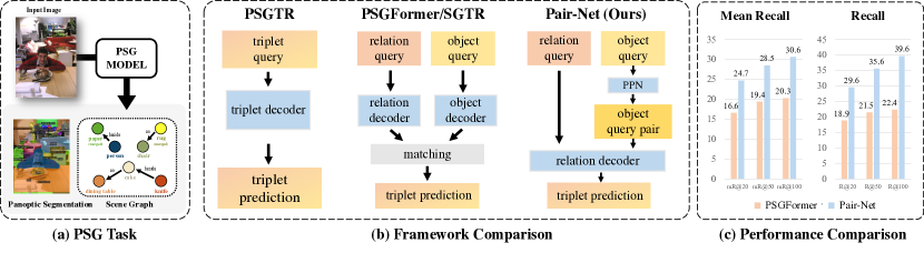
Figure 1: An illustration of Panoptic Scene Graph (PSG) task, framework and performance comparisons. (a) The Panoptic Scene Graph (PSG) task involves generating object-background relations and their masks. (b) Frameworks compared include PSGTR [1], PSGFormer [1], and SGTR [2]. Our Pair-Net uses Pair Proposal Network (PPN) to learn object query pairs first, and then extract relations between targeted subjects and objects. (c) Performance comparison shows significant improvement over previous methods, demonstrating the effectiveness of Pair-Net.

Scene graph generation (SGG) [3] is an essential task in scene understanding that involves generating a graph-structured representation from an input image. This representation captures the locations of a pair of objects (a subject and an object) and their relationship, forming a higher-level abstraction of the image content. SGG has become a fundamental component of several downstream tasks, including image captioning [4, 5, 6, 7], visual question answering [8, 9, 10], and visual reasoning [11, 12].

However, current box-based SGG approaches suffer from two primary limitations. Firstly, they rely on a coarse object localization provided by a bounding box, which may include noisy foreground pixels belonging to one class. Secondly, they do not consider the relationships between background stuff and their context, which is a crucial aspect of scene understanding. To address these limitations, Panoptic Scene Graph generation (PSG) was proposed [1]. PSG, as depicted in Figure 1(a), leverages a more fine-grained scene mask representation and defines relationships for background stuff, thus offering a more comprehensive understanding of the scene. PSG also provides two one-stage baseline methods, PSGTR and PSGFormer, depicted in Figure 1(b). Although these methods outperform their two-stage counterparts, their average (triplet) recall rates are only around 10%. The unsatisfactory performance could fall short of the requirements for downstream applications.

To identify the bottlenecks of the current PSG one-stage models [1], we conducted an in-depth analysis of the calculation of the main recall@K protocol [1] of the PSG task. Notice that a successful recall requires a mask-based IOU of over 0.5 for both the subject and object and correct classifications for all elements in the triplet {Subject, Relation, Object}, we firstly investigated the segmentation quality of query-based segmenters for isolated subjects/objects to determine their impact on PSG performance. Our experiments demonstrate that a query-based segmenter can recall individual subjects/objects satisfactorily, even without relation training. Therefore, we naturally turn to conjecture that the connectivity of subjects and objects, specifically the recall of subject-object pairing, may affect PSG performance. We obtain evidence for this assumption from experimental results, indicating that the recall of PSG has a strong positive correlation with pair-wise recall, and the absolute pair recall value is far from saturation, suggesting that improving the accuracy of subject-object pairing may be critical for improving PSG performance. The complete analysis is illustrated in Section 3.2.

These observations motivate us to propose a new framework for PSG tasks with the goal of learning accurate pair-wised relation maps. In this paper, we present Pair-Net, a novel end-to-end PSG framework, as shown in Figure 2. In Pair-Net, we first apply a query-based segmenter to generate panoptic segmentation for subjects/objects and corresponding object queries without bells and whistles. We then design a Pair-Proposal Network (PPN) that models the object-level interactions between each object, taking the encoded object queries from the segmenter as input and producing feasible subject-object pairs. By systematic analysis of the statistics from the existing scene graph datasets, we notice the strong sparsity of pair-wised relations, which may hinder learning. To acquire sparse and feasible object pairs, we employ a matrix learner to filter the dense pairing relationship map into a considerably sparse one. The frequency count from the ground truth scene graph is used to supervise the output of the matrix learner, significantly improving the sparsity of the filtered map. Based on the filtered map, we select Top-K subject-object pairs as inputs to our Relation Fusion module, which predicts the relations from the context information in the given pairs. This module utilizes context information from subject-object pairs and facilitates interactions through a cross-attention mechanism. In this way, we eventually generate {Subject, Relation, Object} triplets.

We also conduct comprehensive experiments on the PSG dataset. Our method outperforms a strong baseline and achieves a new state-of-the-art performance. In particular, as depicted in Figure 1 (c), we achieve over 10.2% improvement compared with PSGFormer [1]. Through extensive studies, we demonstrate the effectiveness and efficiency of our proposed model.

In sum, this paper provides the following valuable contributions to the PSG community in the hope of advancing the research in this field:

1. Comprehensive analysis of pairwise relations in PSG. We find that although the individual recall for the objects is already saturated for the PSG task, pairwise recall is a significant factor for final recall through systematic experiments.

2. A novel strategy pair-then-relation for solving PSG task. We explore the pair and then relation generation order and propose a simple but effective PPN for explicit pairing modeling, leading to more precise relationship identification.

3. Significant improvement on all metrics of PSG dataset. Through extensive experiments, Pair-Net outperforms existing PSG methods by a large margin and achieves new state-of-the-art performance on the PSG dataset.

2 Related Work

Scene Graph Generation. The existing works for SGG can be divided into the two-stage pipeline and the one-stage pipeline. The two-stage pipeline generally consists of an object detection part and a pairwise predicate estimation part. Many approaches [13, 14, 15, 16, 17, 18] model the contextual information between objects. However, these methods are constrained by the high time complexity due to the pairwise predicate estimation, which is infeasible in complex scenarios with many objects but few relations. One-stage pipelines [19, 20, 21, 22] focus on the one-stage relation detection. However, many still focus on improving detection performance and do not fully use the sparse and semantic priors for SGG. For query-based methods such as RelPN [23] and Graph-RCNN [18], they generate subject, object, and relation separately and measure triplet compatibility score directly. Also, the ROI-based feature extraction methods make them not able to encode information of stuff. Since the queries given by the segmenter have encoded global semantic information, the relation could be naturally and purely conditioned on the concatenated pair query. Meanwhile, there are also several works for Video Scene Graph Generation  [24, 25, 26, 27, 28] and long-tailed problems [29, 30, 31, 32, 33, 34, 35, 36, 17, 26] in SGG. In summary, the methods SGG only handle instance level relation in coarse box format, which lacks pixel-level fine-grained information.

Panoptic Scene Graph Generation. One core limitation of SGG is the missing reasoning on the background context. Introducing background information into the scene graph generation process using panoptic segmentation not only increases the localization level of the labeling from bounding box to mask but also brings the following three benefits: 1) It addresses and reduces some labeling issues introduced by the de facto SGG datasets, i.e., VG-150 [37]. These issues include noisy and overlapping bounding boxes, redundant (e.g., alongside, besides), and ambiguous labels of the relation, redundant and trivial classes (e.g., woman-has-hair), and inconsistent and repeated labeling of the same objects (creating many isolated nodes in the scene graph). 2) A rich and complete visual understanding of an image could not only restrict to only a subset of pixels but all pixels of the image [38]. Also, the interaction (defined as a relation in the scene graph) between background objects (stuff) and foreground objects (thing) is crucial to the understanding of the scene. Given the example in the PSG paper [1], the pavement region is important for understanding the context but is completely ignored. 3) It increases the difficulty of the SGG task. In SGG, the relation could only be defined between thing and thing. Compared with only 1 kind of relation in SGG, in PSG, the scene graph is much more informative and coherent since it can capture and define a total of 4 kinds of relations: stuff-stuff, thing-stuff, stuff-thing, and thing-thing.

To fill the gap mentioned above, Panoptic Scene Graph Generation [1] is proposed. They propose the PSG dataset along with two baselines, including PSGTR and PSGFormer. PSGTR [1] used a triplet query to model the relations in the scene graph as Subject, Relation, Object pairs, while PSGFormer [1] applied both object query and relation query to model the nodes and edges in the scene graph separately, then applied a relation-based fetching to find the most relevant object queries through some interaction modules to build the scene graph. Nonetheless, without explicit modeling of objects, the triplet pair approaches require heavy hand-designed post-processing modules to merge all triplets into a single graph, which may fail to keep the consistent entity-relation structure. As for relation-based fetching, such an approach is not effective and straightforward.

Panoptic Segmentation. This task unifies the semantic segmentation and instance segmentation into one framework with a single metric named Panoptic Quality (PQ) [38]. Lots of works have been proposed to solve this task with various approaches. However, most works [39, 40, 41, 42, 43] separate thing and stuff prediction as individual tasks. Recently, several approaches [44, 45, 46, 25, 47, 48, 49, 50] unify both thing and stuff prediction as a mask-based set prediction problem. Our method is based on the unified model. However, as shown in Table II, better segmentation quality does not mean a better panoptic scene graph result. We pay more attention to the panoptic scene graph generation, with the main focus on pair-wised relation detection.

Detection Transformer. Starting from DETR [51], object query-based detectors [52, 53] are designed using object queries to encode each object and model object detection as a set prediction problem. Several approaches generalize the idea of using object queries for other domains, such as segmentation [54, 46, 44], tracking [55, 56, 57, 58, 25, 49], and scene graph generation [2, 1, 20]. In particular, SS-RCNN [22] uses triplet queries to directly output sparse relation detections. However, the relationship between objects and subjects is not explicitly learned or well explored. Moreover, it can not generalize into PSG directly since the limited mask resolution results by RoI align [59].

3 Methods

In this section, we will first formulate the problem setting of PSG in Section 3.1. Then, we will present our findings from three different aspects in Section 3.2: enough capability of current segmenters, the importance of pair recall, and the sparsity of pair-wise relations. Following this, we will illustrate the detail of our Pair-Net architecture in Section 3.3, including Panoptic Segmentation Network, Pair Proposal Network, and Relation Fusion module. Finally, we will provide the training and inference procedures in Section 3.4.

TABLE I: IoU and Recall_0.5 of COCO-pretrained detectors on PSG. IoU and Recall_0.5 are averaged at the triplet level of the scene graph. It shows the excellency of object-level recall.

Model	sub-IoU	obj-IoU	sub-R0.5	obj-R0.5
DETR [51]	0.74	0.73	0.87	0.84
Mask2Former [44]	0.79	0.78	0.91	0.90

TABLE II: Pair recall@20, triplet recall@20 and PQ of different models on PSG. PSGFormer⁺ denotes that the detector of PSGFormer is changed from DETR to Mask2Former. The table shows that different models have a similar ability in panoptic segmentation (PQ), but Pair Recall is strongly correlated to Triplet Recall.

Model	Pair R@20	R@20	PQ
MOTIFS [14]	36.7	20.0	40.4
VCTree [15]	37.2	20.6	40.4
GPS-Net [16]	34.3	17.8	40.4
PSGFormer [1]	26.6	18.0	36.8
PSGFormer+ [1, 44]	28.6	18.9	43.8
Pair-Net (Ours)	52.7	29.6	40.2

3.1 Problem Setting

A scene graph $\mathbf{S}$ is defined as a set of {Subject, Relation, Object} triplets. In the task of Scene Graph Generation (SGG), the distribution of a scene graph can be summarized in the following two steps:

$$p(\mathbf{S}|\mathbf{I})=p(\mathbf{B},\mathbf{A}|\mathbf{I})p(\mathbf{R}|\mathbf{B},\mathbf{A},\mathbf{I})$$ (1)

Here, $\mathbf{I}\in\mathbb{R}^{H\times W\times 3}$ is the input image, and $\mathbf{B}=\left\{b_{1},\ldots,b_{n}\right\}$ and $\mathbf{A}=\left\{a_{1},\ldots,a_{n}\right\}$ represent the bounding box coordinates and class labels of $n$ objects in the image, respectively. $\mathbf{R}=\left\{r_{1},\ldots,r_{m}\right\}$ represents the relations between objects given $\mathbf{B}$ and $\mathbf{A}$. Here, $a\in\mathbb{Z}^{x}$ and $r\in\mathbb{Z}^{y}$ refer to one of the pre-defined $x$ object and $y$ relation classes. The values of $n$ and $m$ are arbitrary numbers depending on the context of the image.

Instead of localizing only (foreground) objects using the annotation at the level of bounding box coordinates, Panoptic Scene Graph Generation (PSG) grounds each foreground object (thing) with the more fine-grained panoptic segmentation mask annotation. It incorporates information from background objects (stuff) into the consideration of a scene graph. Formally, the model is trained to learn the following distribution:

$$p(\mathbf{S}|\mathbf{I})=p(\mathbf{M},\mathbf{A}|\mathbf{I})p(\mathbf{R}|\mathbf{M},\mathbf{A},\mathbf{I})$$ (2)

In this case, $\mathbf{M}=\left\{m_{1},\ldots,m_{n}\right\}$ and $m_{i}\in{0,1}^{H\times W}$ represent the panoptic segmentation masks corresponding to both foreground and background objects in the image.

Compared to SGG, the difference between $\mathbf{B}$ and $\mathbf{M}$ in Equation 1 and Equation 2 introduces more challenges in PSG. Since all pixels in the image are categorized into specific class labels, it dramatically increases the number of $n$ and $x$, which makes previous RoI-based SGG models [23, 18] fail for this task. Consequently, since relations $r$ are built not only between things and things but between all combinations of things and stuff, the pre-defined relation classes $r\in\mathbb{Z}^{y}$ become more varied and complex, and the generation process of $r$ requires the model to have a more robust and deeper understanding of the image.

3.2 Motivation

Query-based Segmenter is Good Enough for PSG. To learn the pair-wised relation between different entities in PSG, we first study the question, ‘whether the query-based segmenter can encode semantic information of corresponding subject or object using object queries?’ In this way, scene graph generation could be simplified into learning the pair-wised relationship between subjects and objects and classifying object queries to subject and object, respectively. We use COCO-pre-trained models to test both mean mask IoU and Recall of each subject and object depicted in the scene graph. The results, presented in Table I, show that both DETR [51] and Mask2Former [44] are effective in recalling. Given their high Recall_0.5 and IoU, we argue that the quality of panoptic segmentation is already good enough to support the following pair then relation generation, and the performance of PSG models is not bounded by object segmenters. Additionally, this also suggests that object queries, which are used for mask and class prediction, can be utilized as a good predicate to learn the pairwise relationships between entities in PSG directly.

Better Pair Recall, Better Triplet Recall in PSG. In Table II, we test different PSG methods in cases of their recall (main metric of PSG) and pairwise recall. The pair recall is calculated by jointly considering object and subject predictions and omitting the relation classification correctness, which shares the similar thought of Region Proposal Network (RPN) [59] to recall all possible foreground objects. We find pair recall is more important than segmentation quality, while different methods with similar PQ have various recalls. This motivates us to design a model to directly enhance the recall of PSG in pairs rather than improving segmentation quality, which is already good enough for SGG tasks.

TABLE III: Scene graph statistics on PSG. Connectivity measures the ratio between the number of edges that are selected in a scene graph and the number of all possible edges of objects given an image.

Dataset	# avg. obj	# avg. rel	connectivity
VG-150 [37]	10.6	5.7	8.9%
PSG [1]	11.0	5.6	13.5%

Property of Pairing: Sparsity. To further explore the property of pairs in the dataset, we calculate statistics and find an important characteristic: sparsity. The number of edges of a complete graph $C$ that is formed by $N$ instances is $\frac{N(N-1)}{2}$, denoted as $|E|_{C}$. And, we denote the number of edges of the scene graph as $|E|_{sg}$. We define the connectivity in Table III as the ratio between $|E|_{sg}$ and $|E|_{C}$, which could be used as a sparsity measurement. Following mathematical reduction, it could also represent the average proportion of nodes that one node is connected with. As shown in Table III, we find that the connectivity of PSG is 13.5%, which indicates that it is a very sparse dataset. To be specific, on average, one object connects with one object in the graph $C$. This observation strongly motivates us for the design of Matrix Learner and the supervision in Section 3.3.2, to handle the sparsity of the data.

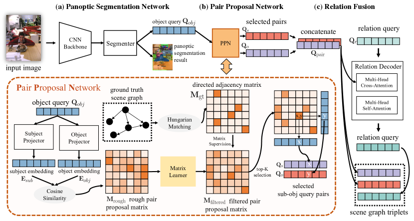
Figure 2: An illustration of our proposed Pair-Net. It mainly contains three parts: (a) Panoptic Segmentation Network uses a query-based object segmenter to generate panoptic segmentation and object queries. (b) Pair Proposal Network generates subject-object pairs from object queries, with Matrix Learner to ensure the sparsity property. (c) Relation Fusion module models the interaction between pair-wised queries and relation queries and predicts final relation labels.

3.3 Pair-Net Architecture

As shown in Figure 2, our Pair-Net mainly contains three parts. Firstly, we use the Mask2Former baseline to extract the object queries. Then we use the proposed Pair Proposal Network to recall all confident subject-object pairs and select the best pairs. Finally, we use the Relation Fusion module to decode the final relation prediction between subjects and objects.

3.3.1 Panoptic Segmentation Network

We adopt strong Mask2Former [44] as our segmenter in the panoptic segmentation network. Mask2Former contains a transformer encoder-decoder architecture with a set of object queries, where the object queries interact with encoder features via masked cross-attention. Unlike RelPN [23] separately generates proposals for subjects, objects, and relations with bounding boxes using 3 branches, the segmenter jointly produces panoptic segmentation of the subjects and objects, without consideration of relation. Given an image $\mathbf{I}$, during the inference, the Mask2Former directly outputs a set of object queries $\mathbf{Q_{\text{obj}}}=q_{\{i\}},i=1\ldots N$, where each object query $q_{i}$ represent one entity. We denote it as $\mathbf{Q}_{\text{obj}}\in\mathbb{R}^{N_{\text{obj}}\times d}$, where $N_{obj}$ is the number of object queries and $d$ is the embedding dimensions. Each object query is matched to ground truth masks during training via masked-based bipartite matching. The loss function is $\mathcal{L}_{\text{mask}}=\lambda_{cls}\mathcal{L}_{cls}+\lambda_{ce}\mathcal{L}_{ce}+\lambda_{dice}\mathcal{L}_{dice}$, where $\mathcal{L}_{cls}$ is Cross Entropy (CE) loss for mask classification, and $\mathcal{L}_{ce}$ and $\mathcal{L}_{dice}$ are CE loss and Dice loss [60] for segmentation, respectively.

3.3.2 Pair Proposal Network

Our Pair Proposal Network (PPN) focuses on predicting the relative importance of subject/object queries and then selects top-k subject-object pairs according to the index of the top-k value in the pair proposal matrix.

As shown in Figure 2, our PPN consists of a subject projector, an object projector, and a matrix learner. The projector layer is an MLP that will generate subject and object embedding $\mathbf{E}_{\text{sub}},\ \mathbf{E}_{\text{obj}}\in\mathbb{R}^{N_{\text{obj}}\times d}$ respectively from input $\mathbf{Q}_{\text{obj}}$. After that, cosine similarity between $\mathbf{E}_{\text{sub}}$ and $\mathbf{E}_{\text{obj}}$ is calculated, i.e., a rough sketch of Pair Proposal Matrix $\mathbf{M}_{\text{rough}}\in\mathbb{R}^{N_{\text{obj}}\times N_{\text{obj}}}$. Finally, a Matrix Learner is applied to further filter the rough sketch of Pair Proposal Matrix $\mathbf{M}_{\text{rough}}$, generating a more precise prediction of importance in the Pair Proposal Matrix. To avoid ambiguity, such interaction is the pairing step between objects, following our pair-then-relation generation order. It is not relevant to the design of RelPN [23], which directly calculates the visual and spatial compatibility among subjects, objects, and relations.

Matrix Learner. Taking the motivation from Section 3.2, a small network, namely matrix learner, is designed to do further filtration and learn feasible sparse pairs. In particular, we find using simple CNN architecture could achieve better results. Rather than using transformer architecture like ViT [61], we argue that a CNN architecture can well preserve the local details while filtering the redundant noise, as a role of an efficient semantic filter. Its output is a filtered pair proposal matrix $\mathbf{M}_{\text{filtered}}$, which contains the sparser connectivity representation compared to its input matrix $\mathbf{M}_{\text{rough}}$. Finally, a top-k selection is conducted on the $\mathbf{M}_{\text{filtered}}$ to select relatively important subject-object pairs for further relation fusion. They are annotated as $\mathbf{Q}_{s}$ and $\mathbf{Q}_{o}$ respectively. We present detailed ablation studies in the experiment section and visualization of $\mathbf{M}_{\text{filtered}}$ and $\mathbf{M}_{\text{rough}}$ in the visualization section.

To supervise the filtration process of the matrix learner, we introduce additional information about pair-wised relations from the ground truth, which is defined as $\mathbf{M}_{\text{gt}}\in\mathbb{R}^{N_{\text{obj}}\times N_{\text{obj}}}$. Using Hungarian matching, we are able to assign each subject and object in the ground truth scene graph to a specific object query $q_{k}$ based on their segmentation losses. After all ground truth subject-object pairs have been assigned, multiple positions of $\mathbf{M}_{\text{gt}}$ will be assigned to $1$ and the remaining positions will be assigned to $0$.

We use such a matrix to supervise the Matrix Learner with a Binary Cross Entropy loss (BCE). Due to the sparsity of $\mathbf{M}_{\text{gt}}$, We enhance the BCE loss with a positive weight adjustment to ensure stable training. This loss forces the network to produce sparse relationships for both subject and object pairs and we derive our proposal pair loss as:

$$\mathcal{L}_{\mathbf{ppn}}=\text{BCE}(\textbf{M}_{\text{gt}},\text{Sigmoid}(\textbf{M}_{\text{filtered}})).$$ (3)

3.3.3 Relation Fusion

After selecting the top-k queries, we adopt another Transformer decoder to predict their relations. As shown in Figure 2 (c), we term it as Relation Fusion. In this module, we have a relation decoder consisting of transformer decoders in the style of [51]. After selecting sub-query $\mathbf{Q}_{s}$ and obj-query $\mathbf{Q}_{o}$ from the object query $\mathbf{Q}_{\text{obj}}$ via PPN, they are concatenated together to construct a pair query $\mathbf{Q}_{\text{pair}}\in\mathbb{R}^{N_{\text{rel}}\times 2d}$, which are projected as the key and value of cross attention in the relation decoder. We initialize a relation query $\mathbf{Q}_{r}\in\mathbb{R}^{N_{\text{rel}}\times d}$ as the query input. $N_{\text{rel}}$ denotes the number of relation queries and $d$ denotes the embedding size of the decoder.

The cross attention mechanism [62] between $\mathbf{Q}_{r}$ and $\mathbf{Q}_{\text{pair}}$ yields an equivalent matching effect through the dot product in the attention formulation. Such that, the $i^{\text{th}}$ relation query mainly pays its attention to the $i^{\text{th}}$ of the $\mathbf{Q}_{\text{pair}}$ while still gaining some information from the other pairs. Since the relation query is in the same order as the pair query, no further post-processing or matching between pairs and relations is needed in this stage. We annotate the Cross-Entropy (CE) loss of subject and object classification as $\mathcal{L}_{s}$, $\mathcal{L}_{o}$, and relation classification loss as $\mathcal{L}_{r}$ respectively.

3.4 Training and Inference

Long-tailed Distribution on Relation. As SGG tasks, we have observed a long-tailed distribution of relation classes, which can heavily affect the performance of mean AR. From Figure 3, we notice that half of the relation classes (tail classes) only account for about $1\%$ and eight classes (head classes) account for about $80\%$ in the training set in PSG. This clearly indicates the characteristic of a long-tailed distribution. There are several methods to handle long-tailed distributions. At the dataset level, resampling of the original dataset with logit adjustment of relation classes can be applied, generating an augmented dataset with a more balanced distribution of relations. At the loss level, Focal Loss [63] modifies the standard cross entropy loss and applies weighted discrimination on the well-classified classes, which forces the model to focus on wrongly classified classes. Furthermore, Seesaw loss [64] dynamically re-balances gradients of positive and negative samples, which is adopted for relation classification in our framework by default. All these different methods will affect the performance of relation loss $\mathcal{L}_{r}$.

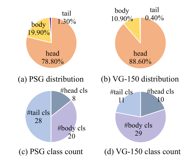
Figure 3: Relation classes distribution of PSG and VG-150. Following [17], we summarize the proportion and number of different classes in the form of head, body, tail of PSG in (a) and (c). We provide results of VG-150 in (b) and (d) for reference. The figure shows the long-tail effect on the distribution of relation classes.

Training Loss. Our Pair-Net can be trained end-to-end as one-stage SGG models. The entire loss contains three classification losses for the subject, object, and relation, one binary classification loss for PPN, and the origin mask loss of Mask2Former. Overall, the loss of our framework is defined as:

$$\mathcal{L}=\lambda_{\text{s}}\mathcal{L}_{\text{s}}+\lambda_{\text{o}}\mathcal{L}_{\text{o}}+\lambda_{\text{r}}\mathcal{L}_{\text{r}}+\lambda_{\text{pp}}\mathcal{L}_{\text{pp}}+\lambda_{\text{mask}}\mathcal{L}_{\text{mask}}.$$ (4)

where we set $\lambda_{\text{o}}=\lambda_{\text{s}}=4,\lambda_{\text{r}}=2,\lambda_{\text{pp}}=5,\lambda_{\text{mask}}=1$.
Inference. The model takes an image as input. Firstly, the segmenter produces object queries $\mathbf{Q}_{\text{obj}}$, the object classification result, and the mask segmentation result. Then, the PPN selects obj-query $\mathbf{Q}_{o}$ and sub-query $\mathbf{Q}_{s}$ based on the top-k index of the filtered pair proposal matrix $\mathbf{M}_{\text{filtered}}$. After concatenation, the selected $\mathbf{Q}_{o}$ and $\mathbf{Q}_{s}$ form as pair query $\mathbf{Q}_{\text{pair}}$ as the key and value function of the relation decoder. Finally, the relation decoder produces a relation query, which is fed into a one-layer perceptron for relation classification. The result triplets are given by the concatenation of subject, object, and relation classification results.

TABLE IV: Different setting comparison with previous SGG and PSG methods.

Method	SGG	PSG	End-to-end	Sparsity	Pair Loss	Background
RelPN [23]	✓
Graph-RCNN [18]	✓			✓
SGTR [2]	✓		✓	✓
PSGTR [1]		✓	✓			✓
PSGFormer [1]		✓	✓			✓
Pair-Net (Ours)	✓	✓	✓	✓	✓	✓

TABLE V: Results on PSG validation dataset. Pair-Net outperforms previous methods by a large margin on all metrics. Our model outperforms prior state-of-the-art models by an absolute 10.2% in mR@20 and 11.6% in R@20.

BackBone	Detector	Model	mR@20	mR@50	mR@100	R@20	R@50	R@100
ResNet-50 [65]	Faster R-CNN [59]	IMP [13]	6.5	7.1	7.2	16.5	18.2	18.6
		MOTIFS [14]	9.1	9.6	9.7	20.0	21.7	22.0
		VCTree [15]	9.7	10.2	10.2	20.6	22.1	22.5
		GPS-Net [16]	7.0	7.5	7.7	17.8	19.6	20.1
	DETR [51]	PSGFormer [1]	14.5	17.4	18.7	18.0	19.6	20.1
	Mask2Former [44]	PSGFormer+ [1]	16.6	19.4	20.3	18.9	21.5	22.4
		Pair-Net (Ours)	24.7	28.5	30.6	29.6	35.6	39.6
Swin-B [66]		Pair-Net† (Ours)	25.4	28.2	29.7	33.3	39.3	42.4

3.5 Relation With Previous SGG Methods

We provide more detailed description and comparison of Pair-Net in Table IV with several feature comparison. Compared with previous works, our proposed Pair-Net support both SGG and PSG, which is also an end-to-end framework. Moreover, we adopt pair loss to drectly optimize the relation different object and subject pairs, which is different from all previous works. As a result, our method lead to sparsity in relation pair within query-based framework. Compared with ReIPN [23] and Graph-RCNN [18], our method also consider the background context.

4 Experiment

Panoptic Scene Graph (PSG) Benchmark [1]. Filtered from COCO [67] and VG datasets [37], the PSG dataset contains 133 object classes including things and stuff and 56 relation classes. This dataset has 46k training images and 2k testing images with panoptic segmentation and scene graph annotation. We follow similar data processing pipelines from [1].

Evaluation Metrics. Since our framework generates triplets directly from the object queries outputted by the object detector, the evaluation matrices based on ground-truth object classification and localization labels such as Predicate Classification (PredCls) and Scene Graph Classification (SGCls) are not suitable for our experiments. Instead, we use Scene Graph Generation (SGGen): given an image, the model performs object segmentation and predicts pair-wise relationships between instances simultaneously. The IoU threshold of a correct mask is set to 0.5 and a correct matching means all elements in the triplet {Subject, Relation, Object} are classified correctly. We report recall@K (R@K) and mean recall@K (mR@K) for K $=20,50,100$ following the definition from [15, 68].

Training Configuration. For the panoptic segmentation task in PSG, we use COCO [67] pre-trained Mask2Former as the object segmenter. Our framework is optimized by AdamW [69] with an initial learning rate of $10^{-4}$, a weight decay of $10^{-4}$, and a batch size of $8$. We train Pair-Net for a total of 12 epochs and reduce the learning rate by a factor of 0.1 at epoch 5 and 10. We set all the positional encoding of the query, key, and value in the Relation Fusion module learnable.

General Framework Hyperparameters. We set the number of object queries to $N_{obj}=100$, size of embedding dimensions, $d=256$ inheriting the design of Mask2Former [44]. The subject projector and object projector are both MLPs with three fully connected layers, with embedding dimension $d=256$ and ReLU as the activation function. For the Matrix Learner, we use a 3-layer CNN with 64 inner channels and a 7 by 7 kernel size. The Relation Fusion consists of a 6-layer DETR-style transformer decoder with $d=256$.

Training Environment. We use Pytorch 1.13.1 [70], MMCV 1.7.0 [71], and MMdetection 2.25.1 [72] complied by CUDA 11.7. The pre-trained Mask2Former is provided by the MMdetection model zoo. Training Pair-Net takes approximately 11 hours for 12 epochs using four NVIDIA 24G GeForce RTX 3090 GPU. We apply no mixed precision during training. We set the seed of all experiments as 10086.

4.1 Main Results

Comparison with Baselines. The previous two-stage models, all of them, choose Faster R-CNN [59] as Detectors. For a fair comparison, we create a stronger baseline method based on PSGFormer [1] using Mask2Former as Detector noted as PSGFormer⁺. As shown in Section 3.2, the segmenter can well detect and segment each subject and object, including thing and stuff. In Table V, we apply Recall@20/50/100 and Mean Recall@20/50/100 as our benchmarks. All models use ResNet-50 for a fair comparison. As shown in Table V, our method Pair-Net achieves 29.6% in R@20 and outperforms the baseline by a 10.7% large margin. Additionally, for R@50 and R@100, the margin is even larger, which proves that our methods can better utilize all 100 proposals and provide reasonable and not self-repeated predictions. Considering mean Recall, our method also outperforms previous SOTA with absolute $10.2\sim 11.9$ gain for $K=20,50,100$.

Pair Recall Improvement. In Table II, our Pair-Net also gains significant improvement on the Pair Recall@20 compared with existing methods. A large 24.1% margin on Pair Recall@20 is obtained compared with the baseline method, PSGFormer⁺. This observation strengthens our assumption that Pair Recall is highly correlated to Recall, and it is a current bottleneck for the PSG model performance.

Categorical Recall@K on PSG. In PSG, which benefited from the panoptic segmentation setting, the relation is constructed not only from thing to thing (TT) class but also from stuff to stuff (SS), stuff to thing (ST), and thing to stuff (TS). To this end, we introduce four new different metrics to evaluate the performance of the model further: TT-Recall@K, SS-Recall@K, ST-Recall@K, and TS-Recall@K. They calculate the recall on the four categories independently. From Table VI, our Pair-Net mainly improves the recall of all the cases. Our findings suggest that we should pay more attention to pair recall for PSG rather than improving segmentation quality.

Stronger Backbone for Pair-Net. We train a larger Pair-Net with Swin-Base [66] as the backbone for future research purposes. A larger backbone could further improve the performance of Pair-Net with absolute $\sim 1\%$ in mean recall and $3\sim 4\%$ in Recall. This indicates the scalability of Pair-Net.

TABLE VI: Four categorical Recall (R)@20 in PSG. We introduce four categorical recalls and report the performance in terms of Recall@20.

Model	TT-R@20	TS-R@20	ST-R@20	SS-R@20
PSGFormer [1]	17.2	21.7	14.9	14.7
PSGFormer+ [1, 44]	19.5	21.5	9.5	18.5
Pair-Net (ours)	25.7	31.5	24.2	34.2

TABLE VII: Pair-Net ablation experiments on PSG. We report mean Recall and Recall with K=20, 50. Our settings are marked in gray.

Linear Embed	Matrix Learner	BCE supervision	mR/R@20	mR/R@50
✓	✓	$\times$	0.5 / 0.4	1.3 / 1.2
✓	$\times$	✓	14.8 / 20.5	21.0 / 29.8
$\times$	✓	✓	14.6 / 22.1	17.8 / 27.9
✓	✓	✓	24.7 / 29.6	28.5 / 35.6

((a))

Architecture	# Para	mR/R@20	mR/R@50
MLP	0.2M	13.0 / 18.8	19.4 / 26.1
MHSA	0.3M	20.6 / 28.1	24.8 / 34.9
CNN-tiny	0.2M	24.7 / 29.6	28.5 / 35.6
CNN-base	30M	23.3 / 33.3	28.2 / 39.3

((b))

Method	mR/R@20	mR/R@50
Cross Entropy Loss	15.4 / 29.0	17.0 / 34.0
Weighted Resampling	12.6 / 21.4	17.6 / 29.3
Focal Loss [63]	19.8 / 28.3	22.1 / 33.6
Seesaw Loss [64]	24.7 / 29.6	28.5 / 35.6

((c))

Input	mR/R@20	mR/R@50
random init	7.3 / 0.7	9.8 / 1.0
image features	1.3 / 2.3	2.6 / 4.1
random pairs	1.1 / 1.2	1.9 / 2.8
concat pairs	24.7 / 29.6	28.5 / 35.6

((d))

# Rel-Query	mR/R@20	mR/R@50
50	23.4 / 26.7	29.7 / 35.7
100	24.7 / 29.6	28.5 / 35.6
200	22.3 / 29.7	25.9 / 35.6

((e))

4.2 Ablation Study

Ablation study on each component of PPN. In Figure 3(a), we first perform ablation studies on the effectiveness of each component of PPN. We find that all three components: linear embedding, matrix learner, and the supervision from directed adjacency matrix are all important to the performance. Notably, without the linear embedding, the model will just diverge and not provide any correct prediction. This is because the object queries only contain the category information and ignore the pair-wised information. The embedding heads force the object queries to distinguish between subject and object. As shown in the second-row of Figure 3(a), a similar situation also happens on the BCE supervision part, which provides vital information about the pair distributions that help pair proposal matrix learning. Adding Matrix Learner further improves the performance by filtering unconfident pairs, as shown in the third-row of Figure 3(a).

Different Architectures for Matrix Learner. In Figure 3(b), we compare different types of architectures for the matrix learner. We select multi-layer perceptrons (MLP), multi-head self-attention (MHSN), and convolutional neural network (CNN-tiny) with model sizes between 0.2M and 0.3M. In addition, we expand the CNN-tiny to CNN-base by two magnitudes (30M) for further comparison. Comparing MLP and attention, CNN achieves the best results since the CNN-based matrix learner can filter out redundant noise and reserve the local details in the matrix, working as an efficient semantic filter. Moreover, increasing CNN parameters does not bring about major changes in the results, proving that the current scale of Matrix Learner is capable of filtering.

Ablation on Relation Loss. To handle the long-tailed problems in Section 3.4, in Figure 3(c), we explore several balanced loss from the existing methods. We set the cross-entropy loss as the baseline. For Focal Loss [63], we test different settings $\gamma=0,0.5,2$ and report the best one. As shown in that table, we choose the Seasaw Loss [64] for our relation classification loss.

Different Input for Key and Value of the Relation Fusion. In Figure 3(d), we select four different levels of information, from low to high, for the input as key and value function of the relation decoder. Random initialization does not provide useful information, while image features have image-level general features. We also try random subject-object pairs, which have contextual information at the object level but do not have a pair-level structure. For our method, the subject-object pair gives both object-level context and pair-level selection. As shown in Figure 3(d), an input with a more specific and richer context can boost the performance of the whole model.

Different Number of Relation Queries. In Figure 3(e), we adjust the number of relation queries from 100 to 50 and 200. We find that the number of relation queries does not greatly affect the result, and our model is robust to the number of relation queries. We set the relation query number to 100 in our model.

TABLE VIII: More Pair-Net ablation experiments on PSG. We report mean Recall and Recall with K=20, 50. Our settings are marked in gray.

Loss weights ($\lambda_{\text{o}}$/ $\lambda_{\text{s}}$/ $\lambda_{\text{r}}$/ $\lambda_{\text{pp}}$)	mR/R@20	mR/R@50
4 / 4 / 2 / 5	24.7 / 29.6	28.5 / 35.6
4 / 4 / 2 / 10	22.0 / 25.7	26.8 / 32.4
4 / 4 / 4 / 5	23.8 / 27.9	26.2 / 32.6
8 / 8 / 2 / 5	22.2 / 26.5	26.7 / 32.9

((f))

Positive weight adjustment	mR/R@20	mR/R@50
$\times$	0.6 / 1.2	1.2 / 2.3
✓	24.7 / 29.6	28.5 / 35.6

((g))

Effect of different loss weights. In Figure 3(f), we adjust the weights of components in the loss function. We find the influence is not significant. It shows that our model design is robust to different loss weight settings.

Positive Weight Adjustment in BCELoss. The positive weight in the PPN is dynamically calculated by the ratio between the total size of $\mathbf{M}_{gt}$ and the number of positive samples in the $\mathbf{M}_{gt}$ hence it is not a hyperparameter. In Figure 3(g), we validate that performance dramatically decreases given the absence of the positive weight adjustment of the BCELoss.

4.3 Qualitative Results and Visualization

Effect of Pair Proposal Network. In Figure 4, the clear diagonal line in $\mathbf{Q}_{obj}\cdot\mathbf{Q}_{obj}^{\top}$ is absent in all other matrices, suggesting that the pairing process in PPN is not based solely on semantic similarity and showing the necessity of the object/subject embedding projection. After further learning with the Matrix Learner, the matrix gets sparse and prone to reflect relational correlation, which depicts the capability of the Matrix Learner on semantic filtering. But it is unnecessary to reach ground-truth sparsity considering unlabeled but reasonable relations and possibly redundant object queries.

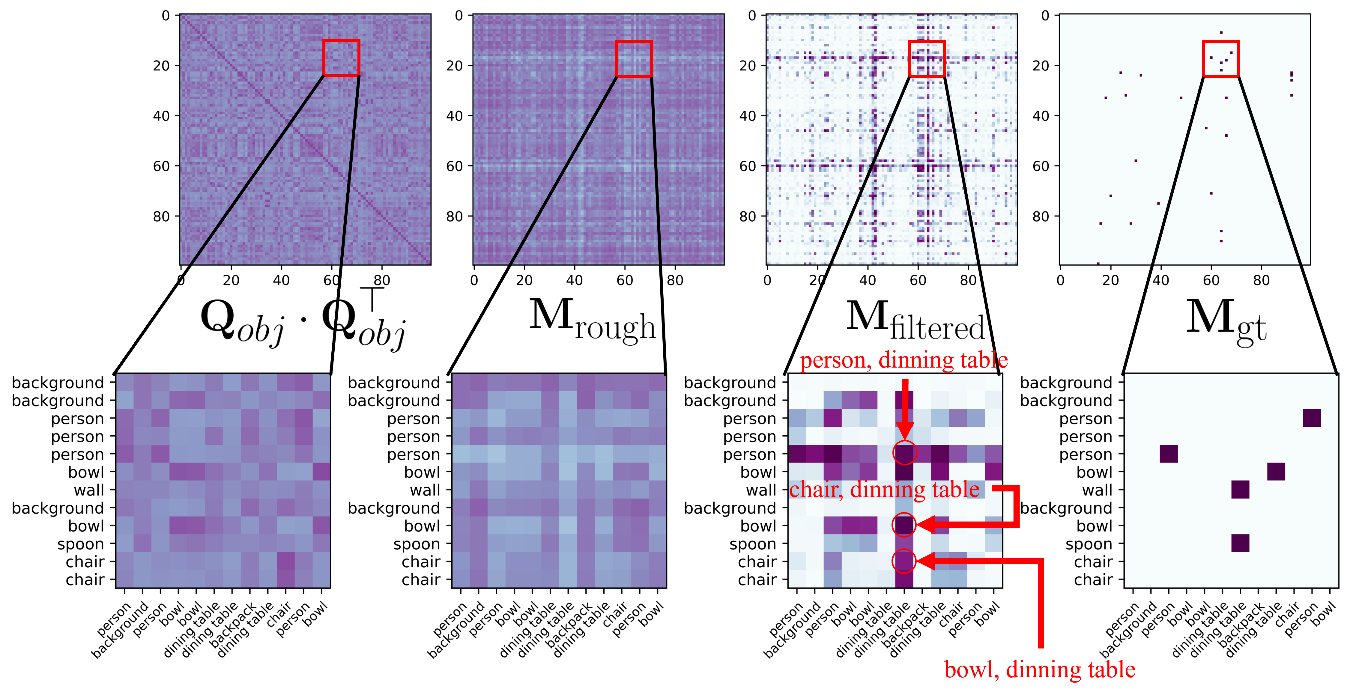
Figure 4: The visualization of Pair Proposal Matrix. Left to right: self-multiplication of object query $\mathbf{Q}_{obj}\cdot\mathbf{Q}_{obj}^{\top}$, $\mathbf{M}_{\text{rough}}$, $\mathbf{M}_{\text{filtered}}$, and $\mathbf{M}_{\text{gt}}$. It reflects that the pairing process in PPN is not based solely on semantic similarity and shows the necessity of the PPN.

Effect of Relation Fusion. In Figure 5, we visualize the averaged cross-attention map of the last layer of the relation decoder. From (a), we notice from values of two diagonals that the $i$-th relation query is heavily weighted from the $i$-th subject query and the $i$-th object query, with minimal information from other queries. From (b) and (c), which shows a $10\times 10$ detailed region from (a) along the diagonals, we can see that the cross attention implicitly performs the matching process between pairs and relation to form the result triplet. This proves the relation fusion module successfully helps relation queries to find the matching subject query and object query.

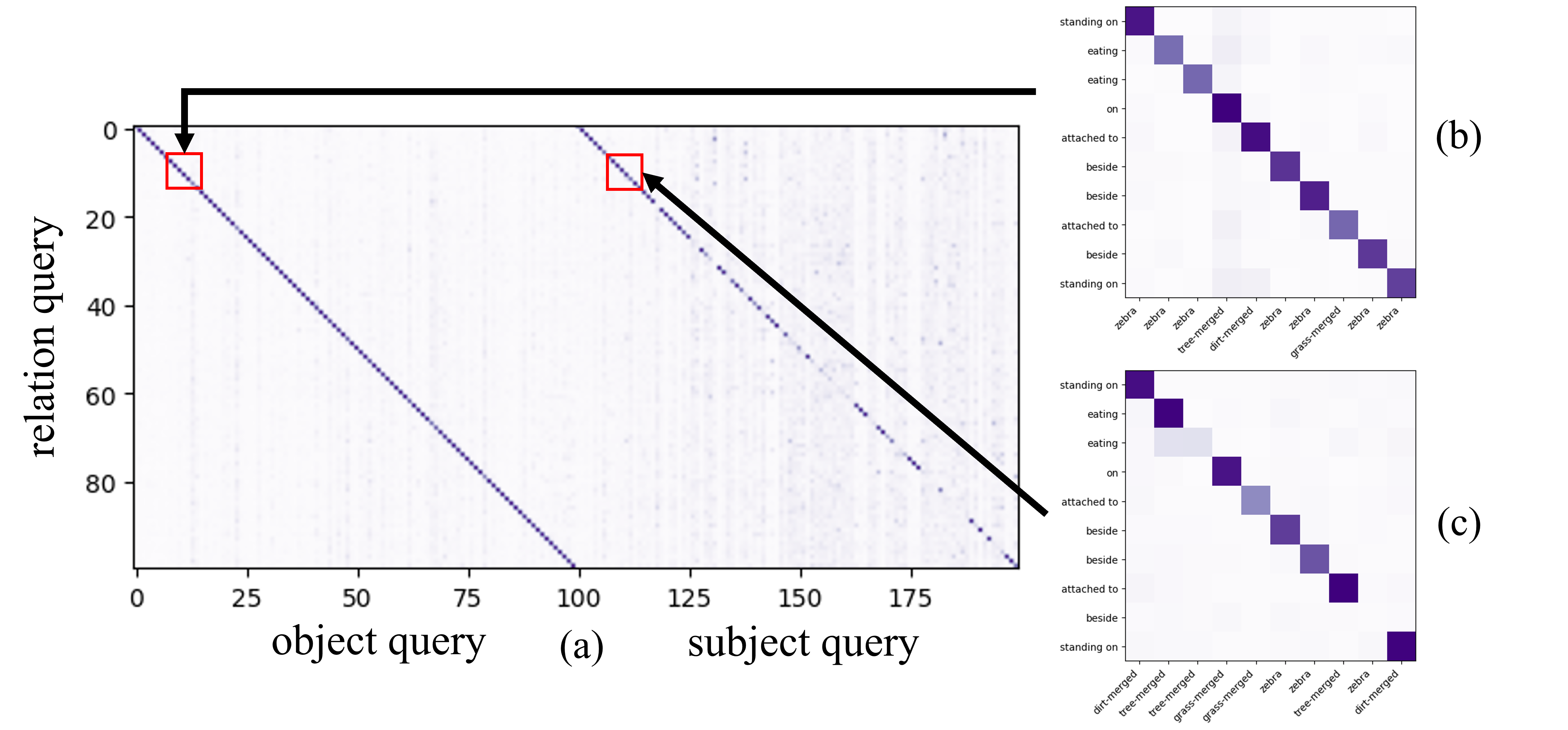
Figure 5: Visualization of the cross-attention map of relation decoder with class annotations. (a) is the overall $N_{\text{rel}}\times 2N_{\text{rel}}$ cross-attention map of the last layer of the relation decoder between the relation query $\mathbf{Q}_{\text{rel}}$ and the pair query $\mathbf{Q}_{\text{pair}}$. (b) and (c) are two selected detailed zones from (a) with class annotations of {Subject, Relation, Object}. The two diagonals in the figure show the strong correlation between the relation query and matched subject / object query.

Visualization of results on PSG. We further visualize the panoptic segmentation and scene graph results for our baseline and Pair-Net. As shown in Figure 6, the results from the baseline model produce many duplications of the same triplets. Such cases downgrade the performance of the model and generate fewer different triplets, thus having lower Recall and Mean Recall. Such duplication case is eliminated in the Pair-Net. This is because of the pair-then-relation approach, which selects the subject-object pair first and does not produce multiple predictions of the same pair.

4.4 Experiments on VG-150

We further report the performance of Pair-Net on VG-150 [37] in Table IX to show that our method could be generalized to a bounding-box-level scene graph dataset and achieves comparable performances with the current specific designed SGG models.

Visual Genome (VG) [37]. We use the most widely used variant of VG [12], namely VG-150, which includes 150 object classes and 50 relation classes. We mainly adopt the data splits and pre-processing from the previous works [13, 14, 17]. After filtering, the VG-150 contains 62k and 26k images for training and testing, respectively.

TABLE IX: Results on VG-150 dataset. Pair-Net achieves comparable performance in recall and mean recall compared with previous transformer-based SOTA works. ’-’ indicates that the data is not reported in the original paper.

Backbone	Detector	Model	mR@20	mR@50	mR@100	R@20	R@50	R@100
VGG[73]	Faster R-CNN[59]	IMP [13]	2.8	4.2	5.3	18.1	25.9	31.2
		MOTIFS [14]	4.1	5.5	6.8	25.1	32.1	36.9
		VCTree [15]	5.4	7.4	8.7	24.5	31.7	36.3
ResNeXt-101 [74]		RelDN [31]	-	6.0	7.3	22.5	31.0	36.7
		GPS-Net [16]	-	7.0	8.6	22.3	28.9	33.2
ResNet-101 [65]	DETR [51]	SGTR [2]	-	12.0	15.2	-	24.6	28.4
	Deformable DETR [53]	Pair-Net-Bbox (Ours)	8.9	12.4	15.4	18.8	24.9	29.3

TABLE X: The performance of object detectors on VG-150. Different models have a similar object detection ability on VG-150 due to the low-quality bounding box label.

Backbone	Detector	Model	AP50
ResNet-101 [65]	DETR [51]	SGTR [2]	31.2
	Deformable DETR [53]	Pair-Net-Bbox (Ours)	31.2

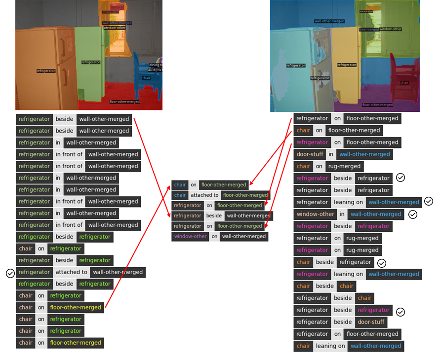
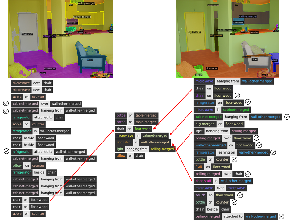
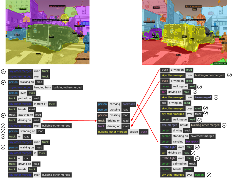
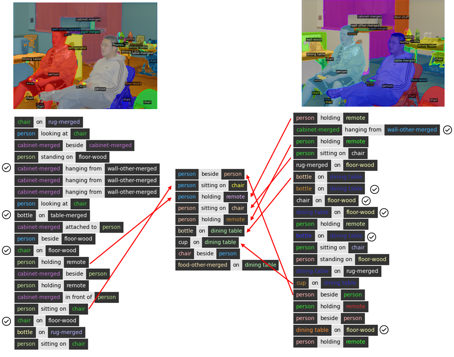
Figure 6: The visualization of scene graph generation of baseline model and Pair-Net. In each image, the left column displays the results from the baseline model, the middle column shows the ground truth, and the right column showcases the results from our proposed Pair-Net.

Training configuration. We fine-tune a 100-query Deformable DETR [53] on VG-150 for the object detection task for 30 epochs. The rest training configurations are the same as training on PSG. To adapt this task, we replace the Mask2Former [44] in Pair-Net to Deformable DETR [53] as the detector, dubbed as Pair-Net-Bbox. We also change the backbone from ResNet-50 to ResNet-101 for a fair comparison with previous work. The rest of the architecture is the same as Pair-Net.

Influence of Object Detector. Shown in Table X, previous SGG SOTA models and ours have a similar ability in object detection in terms of mAP₅₀ on VG-150. Following the previous discussion that the panoptic segmentation performance in terms of PQ is not the key factor to the performance of PSG models, object detection ability is also not the key factor to the performance in SGG task.

Results on VG-150 Benchmark. In Table IX, we apply Recall@20/50/100 and Mean Recall@20/50/100 as our benchmarks. We mainly compare our results with the previous transformer-based VG-150 SOTA model: SGTR [2]. For recall, our methods gain an + 0.3 margin in R@50 and + 0.9 in R@100. Considering mean recall, our method also performs comparably with an additional $0.2\sim 0.4$ improvement. It could be noted that our method is not specially designed for SGG, and we do not perform any extra changes from PSG to SGG. We will put these as our future work.

5 Conclusion

In this work, to tackle the challenging PSG task, we first conduct an in-depth analysis and gain valuable insights for PSG research, and highlight the importance of accurate subject-object pairing. Based on these insights, we propose Pair-Net, a simple and effective framework that achieves state-of-the-art performance on the PSG dataset. We hope this work can help advance research in this field and provide a stronger baseline for PSG’s downstream tasks.

Limitation and Societal Impacts. One limitation of Pair-Net is that we only explore a middle-scale dataset, i.e., PSG. This setting is mainly for a fair comparison with other works [1]. Exploring a larger SGG dataset [75] will be our future work. We hope that other CV domains, like Visual Grounding and Visual Question Answering, can gain some insights from the pair-wised relations.

ACKNOWLEDGMENTS. This work is supported by the National Research Foundation, Singapore under its AI Singapore Programme (AISG Award No: AISG2-PhD-2021-08-019), NTU NAP, MOE AcRF Tier 2 (T2EP20221-0012), and under the RIE2020 Industry Alignment Fund - Industry Collaboration Projects (IAF-ICP) Funding Initiative, as well as cash and in-kind contribution from the industry partner(s).

References

- [1] J. Yang, Y. Z. Ang, Z. Guo, K. Zhou, W. Zhang, and Z. Liu, “Panoptic scene graph generation,” in ECCV (27), 2022.
- [2] R. Li, S. Zhang, and X. He, “SGTR: end-to-end scene graph generation with transformer,” in CVPR, 2022.
- [3] J. Johnson, R. Krishna, M. Stark, L. Li, D. A. Shamma, M. S. Bernstein, and L. Fei-Fei, “Image retrieval using scene graphs,” in CVPR, 2015.
- [4] L. Gao, B. Wang, and W. Wang, “Image captioning with scene-graph based semantic concepts,” in ICMLC, 2018.
- [5] C. Sur, “Tpsgtr: Neural-symbolic tensor product scene-graph-triplet representation for image captioning,” CoRR, 2019.
- [6] S. Chen, Q. Jin, P. Wang, and Q. Wu, “Say as you wish: Fine-grained control of image caption generation with abstract scene graphs,” in CVPR, 2020.
- [7] Y. Zhong, L. Wang, J. Chen, D. Yu, and Y. Li, “Comprehensive image captioning via scene graph decomposition,” in ECCV (14), 2020.
- [8] C. Zhang, W. Chao, and D. Xuan, “An empirical study on leveraging scene graphs for visual question answering,” in BMVC, 2019.
- [9] Z. Yang, Z. Qin, J. Yu, and Y. Hu, “Scene graph reasoning with prior visual relationship for visual question answering,” CoRR, 2018.
- [10] S. Ghosh, G. Burachas, A. Ray, and A. Ziskind, “Generating natural language explanations for visual question answering using scene graphs and visual attention,” CoRR, 2019.
- [11] S. Aditya, Y. Yang, C. Baral, Y. Aloimonos, and C. Fermüller, “Image understanding using vision and reasoning through scene description graph,” Comput. Vis. Image Underst., 2018.
- [12] J. Zhang, Y. Kalantidis, M. Rohrbach, M. Paluri, A. Elgammal, and M. Elhoseiny, “Large-scale visual relationship understanding,” in AAAI, 2019.
- [13] D. Xu, Y. Zhu, C. B. Choy, and L. Fei-Fei, “Scene graph generation by iterative message passing,” in CVPR, 2017.
- [14] R. Zellers, M. Yatskar, S. Thomson, and Y. Choi, “Neural motifs: Scene graph parsing with global context,” in CVPR, 2018.
- [15] K. Tang, H. Zhang, B. Wu, W. Luo, and W. Liu, “Learning to compose dynamic tree structures for visual contexts,” in CVPR, 2019.
- [16] X. Lin, C. Ding, J. Zeng, and D. Tao, “Gps-net: Graph property sensing network for scene graph generation,” in CVPR, 2020.
- [17] R. Li, S. Zhang, B. Wan, and X. He, “Bipartite graph network with adaptive message passing for unbiased scene graph generation,” in CVPR, 2021.
- [18] J. Yang, J. Lu, S. Lee, D. Batra, and D. Parikh, “Graph R-CNN for scene graph generation,” in ECCV (1), 2018.
- [19] Z. Tian, C. Shen, H. Chen, and T. He, “FCOS: fully convolutional one-stage object detection,” in ICCV, 2019.
- [20] Q. Dong, Z. Tu, H. Liao, Y. Zhang, V. Mahadevan, and S. Soatto, “Visual relationship detection using part-and-sum transformers with composite queries,” in ICCV, 2021.
- [21] H. Liu, N. Yan, M. S. Mortazavi, and B. Bhanu, “Fully convolutional scene graph generation,” in CVPR, 2021.
- [22] Y. Teng and L. Wang, “Structured sparse R-CNN for direct scene graph generation,” in CVPR, 2022.
- [23] J. Zhang, M. Elhoseiny, S. Cohen, W. Chang, and A. M. Elgammal, “Relationship proposal networks,” in CVPR, 2017.
- [24] Y. Teng, L. Wang, Z. Li, and G. Wu, “Target adaptive context aggregation for video scene graph generation,” in ICCV, 2021.
- [25] X. Li, W. Zhang, J. Pang, K. Chen, G. Cheng, Y. Tong, and C. C. Loy, “Video k-net: A simple, strong, and unified baseline for video segmentation,” in CVPR, 2022.
- [26] L. Xu, H. Qu, J. Kuen, J. Gu, and J. Liu, “Meta spatio-temporal debiasing for video scene graph generation,” in ECCV (27), 2022.
- [27] K. Gao, L. Chen, Y. Niu, J. Shao, and J. Xiao, “Classification-then-grounding: Reformulating video scene graphs as temporal bipartite graphs,” in CVPR, 2022.
- [28] J. Yang, W. Peng, X. Li, Z. Guo, L. Chen, B. Li, Z. Ma, K. Zhou, W. Zhang, C. C. Loy et al., “Panoptic video scene graph generation,” in CVPR, 2023.
- [29] K. Tang, Y. Niu, J. Huang, J. Shi, and H. Zhang, “Unbiased scene graph generation from biased training,” in CVPR, 2020.
- [30] J. Yu, Y. Chai, Y. Wang, Y. Hu, and Q. Wu, “Cogtree: Cognition tree loss for unbiased scene graph generation,” in IJCAI, 2021.
- [31] J. Zhang, K. J. Shih, A. Elgammal, A. Tao, and B. Catanzaro, “Graphical contrastive losses for scene graph parsing,” in CVPR, 2019.
- [32] A. K. Menon, S. Jayasumana, A. S. Rawat, H. Jain, A. Veit, and S. Kumar, “Long-tail learning via logit adjustment,” in ICLR, 2021.
- [33] S. Abdelkarim, A. Agarwal, P. Achlioptas, J. Chen, J. Huang, B. Li, K. Church, and M. Elhoseiny, “Exploring long tail visual relationship recognition with large vocabulary,” in ICCV, 2021.
- [34] G. Yang, J. Zhang, Y. Zhang, B. Wu, and Y. Yang, “Probabilistic modeling of semantic ambiguity for scene graph generation,” in CVPR, 2021.
- [35] Y. Guo, L. Gao, X. Wang, Y. Hu, X. Xu, X. Lu, H. T. Shen, and J. Song, “From general to specific: Informative scene graph generation via balance adjustment,” in ICCV, 2021.
- [36] M. Chiou, H. Ding, H. Yan, C. Wang, R. Zimmermann, and J. Feng, “Recovering the unbiased scene graphs from the biased ones,” in ACM Multimedia, 2021.
- [37] R. Krishna, Y. Zhu, O. Groth, J. Johnson, K. Hata, J. Kravitz, S. Chen, Y. Kalantidis, L. Li, D. A. Shamma, M. S. Bernstein, and L. Fei-Fei, “Visual genome: Connecting language and vision using crowdsourced dense image annotations,” Int. J. Comput. Vis., 2017.
- [38] A. Kirillov, K. He, R. Girshick, C. Rother, and P. Dollár, “Panoptic segmentation,” in CVPR, 2019.
- [39] B. Cheng, M. D. Collins, Y. Zhu, T. Liu, T. S. Huang, H. Adam, and L. Chen, “Panoptic-deeplab: A simple, strong, and fast baseline for bottom-up panoptic segmentation,” in CVPR, 2020.
- [40] Y. Li, H. Zhao, X. Qi, Y. Chen, L. Qi, L. Wang, Z. Li, J. Sun, and J. Jia, “Fully convolutional networks for panoptic segmentation with point-based supervision,” IEEE Trans. Pattern Anal. Mach. Intell., 2023.
- [41] A. Kirillov, R. B. Girshick, K. He, and P. Dollár, “Panoptic feature pyramid networks,” in CVPR, 2019.
- [42] Y. Xiong, R. Liao, H. Zhao, R. Hu, M. Bai, E. Yumer, and R. Urtasun, “Upsnet: A unified panoptic segmentation network,” in CVPR, 2019.
- [43] Y. Wu, G. Zhang, H. Xu, X. Liang, and L. Lin, “Auto-panoptic: Cooperative multi-component architecture search for panoptic segmentation,” in NeurIPS, 2020.
- [44] B. Cheng, I. Misra, A. G. Schwing, A. Kirillov, and R. Girdhar, “Masked-attention mask transformer for universal image segmentation,” in CVPR, 2022.
- [45] W. Zhang, J. Pang, K. Chen, and C. C. Loy, “K-net: Towards unified image segmentation,” in NeurIPS, 2021.
- [46] B. Cheng, A. G. Schwing, and A. Kirillov, “Per-pixel classification is not all you need for semantic segmentation,” in NeurIPS, 2021.
- [47] H. Yuan, X. Li, Y. Yang, G. Cheng, J. Zhang, Y. Tong, L. Zhang, and D. Tao, “Polyphonicformer: Unified query learning for depth-aware video panoptic segmentation,” in ECCV, 2022.
- [48] X. Li, S. Xu, Y. Yang, H. Yuan, G. Cheng, Y. Tong, Z. Lin, and D. Tao, “Panopticpartformer++: A unified and decoupled view for panoptic part segmentation,” CoRR, 2023.
- [49] X. Li, H. Yuan, W. Zhang, G. Cheng, J. Pang, and C. C. Loy, “Tube-link: A flexible cross tube baseline for universal video segmentation,” ICCV, 2023.
- [50] Y. Han, J. Zhang, Z. Xue, C. Xu, X. Shen, Y. Wang, C. Wang, Y. Liu, and X. Li, “Reference twice: A simple and unified baseline for few-shot instance segmentation,” arxiv, 2023.
- [51] N. Carion, F. Massa, G. Synnaeve, N. Usunier, A. Kirillov, and S. Zagoruyko, “End-to-end object detection with transformers,” in ECCV, 2020.
- [52] P. Sun, R. Zhang, Y. Jiang, T. Kong, C. Xu, W. Zhan, M. Tomizuka, L. Li, Z. Yuan, C. Wang, and P. Luo, “Sparse R-CNN: end-to-end object detection with learnable proposals,” in CVPR, 2021.
- [53] X. Zhu, W. Su, L. Lu, B. Li, X. Wang, and J. Dai, “Deformable DETR: deformable transformers for end-to-end object detection,” in ICLR, 2021.
- [54] H. Wang, Y. Zhu, H. Adam, A. L. Yuille, and L. Chen, “Max-deeplab: End-to-end panoptic segmentation with mask transformers,” in CVPR, 2021.
- [55] M. Chen, Y. Liao, S. Liu, Z. Chen, F. Wang, and C. Qian, “Reformulating HOI detection as adaptive set prediction,” in CVPR, 2021.
- [56] B. Kim, J. Lee, J. Kang, E. Kim, and H. J. Kim, “HOTR: end-to-end human-object interaction detection with transformers,” in CVPR, 2021.
- [57] F. Zeng, B. Dong, Y. Zhang, T. Wang, X. Zhang, and Y. Wei, “MOTR: end-to-end multiple-object tracking with transformer,” in ECCV (27), 2022.
- [58] P. Sun, Y. Jiang, R. Zhang, E. Xie, J. Cao, X. Hu, T. Kong, Z. Yuan, C. Wang, and P. Luo, “Transtrack: Multiple-object tracking with transformer,” CoRR, 2020.
- [59] S. Ren, K. He, R. B. Girshick, and J. Sun, “Faster R-CNN: towards real-time object detection with region proposal networks,” IEEE Trans. Pattern Anal. Mach. Intell., 2017.
- [60] F. Milletari, N. Navab, and S. Ahmadi, “V-net: Fully convolutional neural networks for volumetric medical image segmentation,” in 3DV, 2016.
- [61] A. Dosovitskiy, L. Beyer, A. Kolesnikov, D. Weissenborn, X. Zhai, T. Unterthiner, M. Dehghani, M. Minderer, G. Heigold, S. Gelly, J. Uszkoreit, and N. Houlsby, “An image is worth 16x16 words: Transformers for image recognition at scale,” in ICLR, 2021.
- [62] A. Vaswani, N. Shazeer, N. Parmar, J. Uszkoreit, L. Jones, A. N. Gomez, Ł. Kaiser, and I. Polosukhin, “Attention is all you need,” NeurIPS, 2017.
- [63] T. Lin, P. Goyal, R. B. Girshick, K. He, and P. Dollár, “Focal loss for dense object detection,” in ICCV, 2017.
- [64] J. Wang, W. Zhang, Y. Zang, Y. Cao, J. Pang, T. Gong, K. Chen, Z. Liu, C. C. Loy, and D. Lin, “Seesaw loss for long-tailed instance segmentation,” in CVPR, 2021.
- [65] R. Ferjaoui, M. A. Cherni, F. Abidi, and A. Zidi, “Deep residual learning based on resnet50 for COVID-19 recognition in lung CT images,” in CoDIT, 2022.
- [66] Z. Liu, Y. Lin, Y. Cao, H. Hu, Y. Wei, Z. Zhang, S. Lin, and B. Guo, “Swin transformer: Hierarchical vision transformer using shifted windows,” in ICCV, 2021.
- [67] T. Lin, M. Maire, S. J. Belongie, J. Hays, P. Perona, D. Ramanan, P. Dollár, and C. L. Zitnick, “Microsoft COCO: common objects in context,” in ECCV (5), 2014.
- [68] T. Chen, W. Yu, R. Chen, and L. Lin, “Knowledge-embedded routing network for scene graph generation,” in CVPR, 2019.
- [69] I. Loshchilov and F. Hutter, “Decoupled weight decay regularization,” in ICLR (Poster), 2019.
- [70] A. Paszke, S. Gross, F. Massa, A. Lerer, J. Bradbury, G. Chanan, T. Killeen, Z. Lin, N. Gimelshein, L. Antiga, A. Desmaison, A. Köpf, E. Z. Yang, Z. DeVito, M. Raison, A. Tejani, S. Chilamkurthy, B. Steiner, L. Fang, J. Bai, and S. Chintala, “Pytorch: An imperative style, high-performance deep learning library,” in NeurIPS, 2019.
- [71] M. Contributors, “MMCV: OpenMMLab computer vision foundation,” https://github.com/open-mmlab/mmcv, 2018.
- [72] K. Chen, J. Wang, J. Pang, Y. Cao, Y. Xiong, X. Li, S. Sun, W. Feng, Z. Liu, J. Xu, Z. Zhang, D. Cheng, C. Zhu, T. Cheng, Q. Zhao, B. Li, X. Lu, R. Zhu, Y. Wu, J. Dai, J. Wang, J. Shi, W. Ouyang, C. C. Loy, and D. Lin, “Mmdetection: Open mmlab detection toolbox and benchmark,” CoRR, 2019.
- [73] K. Simonyan and A. Zisserman, “Very deep convolutional networks for large-scale image recognition,” in ICLR, 2015.
- [74] S. Xie, R. B. Girshick, P. Dollár, Z. Tu, and K. He, “Aggregated residual transformations for deep neural networks,” in CVPR, 2017.
- [75] A. Kuznetsova, H. Rom, N. Alldrin, J. R. R. Uijlings, I. Krasin, J. Pont-Tuset, S. Kamali, S. Popov, M. Malloci, A. Kolesnikov, T. Duerig, and V. Ferrari, “The open images dataset V4,” Int. J. Comput. Vis., 2020.