Towards numerical-relativity informed effective-one-body waveforms
for dynamical capture black hole binaries

Abstract

Dynamical captures of black holes may take place in dense stellar media due to the emission of gravitational radiation during a close passage. Detection of such events requires detailed modelling, since their phenomenology qualitatively differs from that of quasi-circular binaries. Very few models can deliver such waveforms, and none includes information from Numerical Relativity (NR) simulations of non quasi-circular coalescences. In this study we present a first step towards a fully NR-informed Effective One Body (EOB) model of dynamical captures. We perform 14 new simulations of single and double encounter mergers, and use this data to inform the merger-ringdown model of the TEOBResumS-Dalì approximant. We keep the initial energy approximately fixed to the binary mass, and vary the mass-rescaled, dimensionless angular momentum in the range $(0.6,1.1)$, the mass ratio in $(1,2.15)$ and aligned dimensionless spins in $(-0.5,0.5)$. We find that the model is able to match NR to $97\%$, improving previous performances, without the need of modifying the base-line template. Upon NR informing the model, this improves to $99\%$ with the exception of one outlier corresponding to a direct plunge. The maximum EOB/NR phase difference at merger for the uninformed model is of 0.15 radians, which is reduced to 0.1 radians after the NR information is introduced. We outline the steps towards a fully informed EOB model of dynamical captures, and discuss future improvements.

I Introduction

The detection and characterization of gravitational waves (GW) requires a multidisciplinary effort that combines instruments of exquisite precision – the LIGO-Virgo-KAGRA (LVK) network of interferometers Aasi et al. (2015); Acernese et al. (2015); Akutsu et al. (2021) – and sophisticated data analysis techniques. Thus far, the most numerous events in the LVK catalogue have been categorized as binary black holes (BBHs) with small or negligible eccentricity Abbott et al. (2021). This type of event is expected to ensue from stellar binaries that have evolved in isolation from their environments and have radiated away their excess angular momentum, thus displaying quasi-circular orbits once they enter the sensitive band. However, some events do not easily fit in this category. In particular, the most massive BBH observed to date, GW190521 Abbott et al. (2020a, b), has been shown to be consistent with a dynamical capture of two nonspinning black holes Gamba et al. (2022). Alternative interpretations of this source are discussed in Romero-Shaw et al. (2020); Bustillo et al. (2021); Gayathri et al. (2022); Shibata et al. (2021).

Dynamical captures may take place in dense stellar media such as globular clusters if the individual black holes radiate gravitational energy during a close passage Rasskazov and Kocsis (2019); Tagawa et al. (2020). Since the phenomenology of these events is sensibly different from the quasi-circular ones Zevin et al. (2019); Samsing and D’Orazio (2018); Nagar et al. (2021a), detailed modeling of the waveforms is required to detect and properly characterize such events through matched filtering. Indeed, if quasi-circular templates are used for the search and analysis of waveforms generated by dynamical captures, the events might be missed or incorrectly analyzed East et al. (2013); Loutrel (2020); Nagar et al. (2021a). Moreover, events of this kind can be detected for farther and heavier black hole systems O’Leary et al. (2009). Dynamical captures are also relevant for next-generation detectors such as LISA Amaro-Seoane (2018) and the Einstein Telescope Punturo et al. (2010). The detectability rate for next-generation, ground-based detectors has been estimated in Ref. Mukherjee et al. (2020).

Numerical Relativity (NR), i.e. the fully fledged evolution of Einstein’s equations, provides the most detailed description of BBH mergers. However, a systematic NR study of dynamical captures is presently missing. Low energy non-spinning encounters have been systematically studied by Gold and Brügmann (2013). Fewer initial data including spin and mass ratio effects have been considered in Refs. East et al. (2013); Nelson et al. (2019); Bae et al. (2020); Gamba et al. (2022). NR simulations for hyperbolic encounters have also been recently considered in Jaraba and Garcia-Bellido (2021) including spin and varying mass ratios. Several new simulations of bound orbits but with large eccentricity and precessing spins have also been recently reported Gayathri et al. (2022); Healy and Lousto (2022). The computational cost involved in spanning the possible orbital configurations for different binaries (mass ratio and spins) makes impractical to directly employ NR for a complete survey and for constructing waveform approximants. Similarly to the circularized orbits case, our strategy is to exploit synergy with analytical relativity.

Reference Nagar et al. (2021a) proposed the first analytical and complete general-relativistic description of the dynamics and waveforms of dynamical captures. The approach of Nagar et al. (2021a) is based on the Effective One Body (EOB) framework TEOBResumS Damour and Nagar (2014); Bernuzzi et al. (2015); Nagar et al. (2017, 2018); Akcay et al. (2019); Nagar et al. (2019, 2020) and in particular on the generic orbits version TEOBResumS-Dalì Chiaramello and Nagar (2020); Nagar et al. (2021b); Nagar and Rettegno (2021). This model was the basis for the analysis of GW190521 reported by Gamba et al. (2022), as well as the eccentric analyses presented in Iglesias et al. (2022). It produces a quantitative predictions for the waveform from the entire orbital parameter space, including spin and mass-ratio effects. Remarkably, despite not being informed by any eccentric NR simulation, TEOBResumS-Dalì shows mismatches below $1\%$ for almost all the available mildly eccentric configurations of the SXS catalog Nagar et al. (2021b) as well as for the RIT catalog Gamba et al. (2022). The accuracy of the EOB dynamics has been also tested in the hyperbolic encounter scenario by comparing the EOB/NR scattering angles for both non-spinning and spinning configurations Damour et al. (2014); Hopper et al. (2022); Damour and Rettegno (2022). Moreover, the accuracy of the fluxes, i.e. the non-conservative part of the dynamics, has been tested both for comparable mass and high-mass ratio systems Albertini et al. (2021, 2022a, 2022b) in the quasi-circular case, and for hyperbolic and eccentric systems with extreme mass ratio Albanesi et al. (2021, 2022a). However, even if a few EOB/NR comparisons for equal mass binaries have been reported in the Supplemental Material of Ref. Gamba et al. (2022), the dynamical capture scenario for comparable mass black holes still needs to be explored in detail. A search for hyperbolic encounters using public data was carried out in Morrás et al. (2022), with results consistent with the false alarm search rate. Observational implications of dynamical captures have recently been considered in Ebersold et al. (2022).

The main goal of this work is to assess the capabilities of the latest version of TEOBResumS-Dalì Nagar et al. (2021b) in the dynamical capture scenario. We carry out a series of new NR simulations of dynamical captures, quantitatively verify some of the key predictions of Nagar et al. (2021a), and propose a first strategy to inform the model with NR data. As we show below, we find that by appropriately informing our model with data coming from NR simulations we are able to obtain waveforms more than $99\%$ faithful to NR in most cases.

This paper is organized as follows: In Sec. II we present our new NR simulations and perform the first comparison between the EinsteinToolkit and GR-Athena++  NR codes. We describe in some detail the configurations chosen, the two codes employed to obtain them and the tests that we performed to ensure convergence. We also discuss the post-processing of the NR data, with a focus on waveform extraction techniques. In Sec. III we briefly introduce the TEOBResumS-Dalì model, discuss the NR-informed parameters that we consider and tackle the issue of connecting NR and EOB initial data. In Sec. IV we perform comparisons between our simulations and TEOBResumS-Dalì, presenting both time-domain phasing comparisons and mismatch computations. Finally, in Sec. V we summarize and discuss our results. Geometric units with $G=c=1$ are employed throughout the text, unless otherwise specified.

II Numerical relativity simulations

II.1 Numerical codes

II.1.1 Einstein Toolkit

For the bulk of this work we use the open source software EinsteinToolkit Löffler et al. (2012). This code is organized as a main driver (Cactus) and a series of modules (thorns) that perform specific tasks. BBH initial data are computed with the TwoPunctures thorn Brandt and Brügmann (1997); Ansorg et al. (2004), which is appropriate to solve the constraint equations on the initial $t=0$ slice for the modest values of spins and mass ratio considered in this work. In the range of parameters we have explored, this algorithm converges to the desired numerical precision within a few iterations. The time evolution is carried out by the MLBSSN thorn which implements the BSSN formulation of vacuum General Relativity Baumgarte and Shapiro (1999); Shibata and Nakamura (1995). We use 6th order finite differences for spatial derivatives and a method-of-lines time integration with a 4th order Runge-Kutta scheme. Moreover, we include Kreiss-Oliger dissipation of order 9 scaled with a factor of $\epsilon=0.1$. The CFL factor for our EinsteinToolkit runs is $0.1$.

Our grid setup consists of a cubic box of edge $L=640M$ (in the coarsest level, the cartesian coordinates range from $-320M$ to $320M$) and spacing at the coarsest level $\delta x=\{3,4,6\}M$, corresponding to (Low, Medium, High) resolutions. Here $M$ is the total mass of the binary, defined as the sum of the individual ADM masses. We have carried out most of our simulations at $\delta x=4M$. We also provide convergence tests for selected simulations consider the low and high resolutions. The code uses Berger-Oliger mesh refinement with 9 overlapping refinement levels in a box-in-box fashion, with the two most refined boxes containing the two punctures. The boxes follow the two punctures, whose position is determined during the evolution with the PunctureTracker thorn. This setting results in a puncture resolution of $\delta x_{p}=4/2^{8}M=0.015625M$. For unequal masses, we add an extra refinement level only at the smaller black hole. This was proven crucial to obtain robust results as we vary resolution. We exploit the reflection symmetry of our configurations to reduce the computational domain by a half in the $z-$direction.

We extract the wave content of our simulations using the thorns WeylScal4 and Multipole which outputs the Weyl scalars $\psi_{4}$ expanded in spherical harmonics up to $\ell=8$, at fixed radius. We check that $R\psi_{4}={\rm const}$, as expected for the extraction radii $R=\left\{70,\,80,\,90,\,100,\,110\right\}\,M$, which are located in a refinement level at the same resolution $\delta x=4/2^{2}M=1M$. On the contrary, extraction radii $R\geq 120$ fall within levels of lower resolution, which causes power loss due to numerical dissipation.

II.1.2 GR-Athena++

In this work we also extend the set of GR-Athena++ Daszuta et al. (2021) simulations presented in Gamba et al. (2022). The initial data are computed with a stand-alone version of the thorn TwoPunctures Brandt and Brügmann (1997); Ansorg et al. (2004). The time evolution is then performed by GR-Athena++ using the Z4c formulation Bona et al. (2003). Moving puncture gauge conditions with the same parameters in Ref. Daszuta et al. (2021) are adopted. As in the EinsteinToolkit case, we use 6th order finite-difference methods for the spatial derivatives and we perform the time-integration using a 4th order Runge-Kutta algorithm. In contrast, for the simulations performed here, Kreiss-Oliger dissipation of order $8$ is included with a factor $\epsilon=0.02$. We also choose a bigger box with edge $L=3072M$, so that in the coarsest level the cartesian coordinates range from $-1536M$ to $1536M$. The AMR in GR-Athena++ is oct-tree based, with the grid organized as an initial Mesh divided into Meshblocks which have all the same number of grid points but (possibly) different physical size. For a cubic initial Mesh and cubic Meshblocks, the grid setup in GR-Athena++ is regulated by three parameters: the number of grid points in the edges of the unrefined initial mesh $N_{M}$, the number of grid points in the edges of Meshblocks $N_{B}$, and the number of physical refinement levels $N_{L}$. The grid structure is ultimately determined by an AMR criterion, which, when satisfied, (de)refines a given MeshBlock, resulting in a (larger) smaller block with (half) double the resolution. For BBH simulations the AMR criterion used mimics the box-in-box strategy mentioned above. In our simulations we consider $N_{B}=16$, $N_{L}=11$, and $N_{M}=\left\{128,\,192,\,256\right\}$. These values are chosen so that the resolution at the punctures is the same as the simulations performed with the EinsteinToolkit code. For all the runs we consider a CFL number of 0.5 The Weyl scalar is then extracted at $R=\left\{80,90,100,110,120,130,140\right\}M$ using an approximate geodesic sphere built using 9002 vertices. For the three grids considered, the resolutions in the extraction zones at the merger time are $\delta x_{R}=\left\{3,2,1.5\right\}M$ for $R>96M$, while they are $\delta x_{R}=\left\{1.5,1,0.75\right\}M$ for $48M<R<96M$. Note that at the beginning of the simulation the extraction zone for $R>96M$ does not have a uniform resolution since the positions of the two punctures make some portions of the zone more refined. We observed that $R\psi_{4}$ remains approximately constant at all the extraction radii, showing that $\psi_{4}$ scales as $1/R$, as expected. More technical details on the structure of the grid and of the geodesic sphere can be found in Ref. Daszuta et al. (2021). Note that no grid-symmetries are employed for these runs.

II.2 Initial data

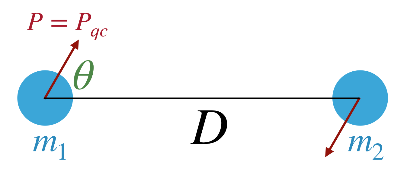
We consider initial data consisting of two black holes of (quasi-local) ADM masses $M_{1}$ and $M_{2}$ separated by a coordinate distance $D$. The total mass of the binary is $M=M_{1}+M_{2}$. We take their ADM linear momenta to be $\vec{P}_{1}=-\vec{P}_{2}$, with $\vec{P}_{1}=P_{qc}(\cos\theta,\sin\theta,0)$ where $P_{qc}$ corresponds to the quasi-circular value. The black holes have spins $\vec{J}_{1}$, $\vec{J}_{2}$ aligned with the orbital angular momenta, so that $\vec{J}_{1}=\chi_{1}M_{1}^{2}(0,0,1)$, $\vec{J}_{2}=\chi_{2}M_{2}^{2}(0,0,1)$. Here $\chi_{1,2}$ are dimensionless spin parameters. Following Gold and Brügmann (2013) we take $D=20M$ which in turn implies $P_{qc}=0.06175M$. See Fig 1 for a schematic depiction of our initial data.

Figure 1: Schematic depiction of our initial data. The initial separation $D$ and the the value of $P$ are kept fixed at $20M$ and $0.06175M$, respectively, and we vary the initial angle $\theta$ as well as the intrinsic spins of the BH components.

II.3 Simulation results

Table 1: Dynamical capture BBHs configurations considered in this work. From left to right the columns report: the configuration name; the mass ratio $q=m_{1}/m_{2}$, the angle $\theta$ of the component of the tangential momentum; the dimensionless spins $\chi_{i}\equiv S_{i}/m_{i}^{2}$, the initial ADM energy and angular momentum, $(E_{0}^{\rm ADM},J_{0}^{\rm ADM})$, the final energy and angular momentum $(E_{f},J_{f})$ and the gravitational wave losses $(\Delta E,\Delta J)$, all expressed in units of the total mass $M$. The initial separation is $D=20M$ for all configurations. All configurations are simulated using the EinsteinToolkit. Those marked with a star also with the GR-Athena++ code. See Table 2 below for additional information.

#	ID	$q$	$\theta$ [deg]	$\chi_{1}$	$\chi_{2}$	$E_{0}^{\rm ADM}/M$	$J_{0}^{\rm ADM}/M^{2}$	$E_{f}/M$	$J_{f}/M^{2}$	$\Delta E_{EOB}/M$	$\Delta J_{EOB}/M^{2}$
1	ETK37q1s0	1.00	37	0.00	0.00	0.99427	0.74321	0.97812	0.65522	0.00000	0.00446
2	ETK42q1s0 ∗	1.00	42	0.00	0.00	0.99427	0.82634	0.96521	0.67555	0.00005	0.00488
3	ETK44q1s0	1.00	44	0.00	0.00	0.99428	0.85786	0.95755	0.66749	0.00000	0.00515
4	ETK46q1s0	1.00	46	0.00	0.00	0.99428	0.88834	0.94903	0.64455	0.00008	0.00486
5	ETK48q1s0 ∗	1.00	48	0.00	0.00	0.99428	0.91774	0.95035	0.60959	0.00009	0.00539
6	ETK50q1s0 ∗	1.00	50	0.00	0.00	0.99429	0.94602	0.94858	0.62682	0.00025	0.00094
7	ETK42q1s025--	1.00	42	$-0.25$	$-0.25$	0.99425	0.70134	0.97564	0.59586	0.00000	0.00421
8	ETK42q1s025++	1.00	42	0.25	0.25	0.99433	0.95134	0.94320	0.70570	0.00000	0.00571
9	ETK42q1s050--	1.00	42	$-0.50$	$-0.50$	0.99439	0.57634	0.98122	0.49612	0.00000	0.00346
10	ETK42q1s050++	1.00	42	0.50	0.50	0.99454	1.07634	0.93980	0.73469	0.00016	0.00606
11	ETK42q1s050+-	1.00	42	0.50	$-0.50$	0.99447	0.82634	0.96517	0.67477	0.00000	0.00496
12	ETK42q1.5s0	1.50	42	0.00	0.00	0.99501	0.82634	0.96229	0.65471	0.00000	0.00496
13	ETK42q2s0	2.00	42	0.00	0.00	0.99641	0.82634	0.95710	0.58005	0.00079	0.00444
14	ETK42q2.15s0	2.15	42	0.00	0.00	0.99687	0.82634	0.96340	0.58504	0.00012	0.00180

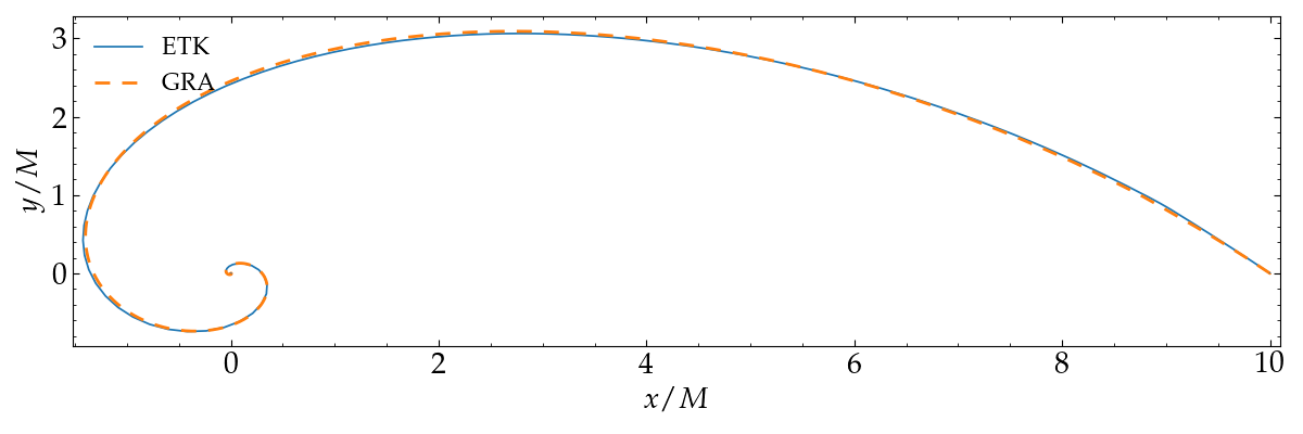
We considered 14 configurations that were simulated using EinsteinToolkit. Table 1 collects the initial physical parameters, while in Appendix A we show the puncture trajectories and the time evolution of the $\ell=m=2$ multipole of the Weyl scalar $\psi_{4}$. Simulations will be refereed to using their ID as defined in the first column of Table 1. The phenomenology of the transition from eccentric inspiral, zoom-whirl behavior and dynamical capture was studied in Ref. Pretorius and Khurana (2007); Gold and Brügmann (2013) as the initial angle $\theta$ is varied. For angles close to $\theta=0$ (head-on collision) one has direct plunges. For fixed values of the initial separation $D$, one can have various close encounters (including zoom-whirl behavior) before the final merger. Finally, for angles $\theta$ beyond a certain threshold, the black hole do not merge and follow hyperbolic trajectories. In our set of simulations, for equal masses and $\theta$ below 48 degrees we find plunges, in ETK37q1s0,42q1s0,44q1s0,46q1s0, while ETK48q1s0 begins to display features of a zoom-whirl which can be fully appreciated in ETK50q1s0. Simulations ETK42q1s0,48q1s0,50q1s0 correspond to some of the configurations presented in Ref. Gold and Brügmann (2013). We find good qualitative and quantitative agreement between puncture tracks and waveforms. These are a plunge, a transition to double encounter and a double encounter, respectively. Note that this agreement is particularly non-trivial for ETK48q1s0, since, due to the fact that this is a boundary case between single and double encounters, slight changes on the initial data or resolution can lead to different results. We further analyze these three cases by performing self-convergence tests and a code comparison between EinsteinToolkit and GR-Athena++, see Sec. II.7.

As also stated in Gold and Brügmann (2013), varying the mass ratio can also result in zoom-whirls. We explore this regime in our series ETK42,42q150,42q200, ETK42q2.15s0, going from a plunge to a fully developed zoom-whirl. Moreover, we have observed that zoom-whirls can be induced by increasing the angular momenta by adding spin to the components of a binary which yields a plunge orbit in the non-spinning case. This is found in our simulations ETK42q1s050--, 42q1s025--, 42q1s0, 42q1s025++, 42q1s050++ as discussed in Sec, IV.1.2 and is analytically explained via the spin-orbit interaction. NR simulations are also known to suffer from “junk radiation” i.e. radiation caused by the underlying conformally flat assumption used for the computation of the initial data. In our case, we observe a small burst of radiation in $\psi_{4}$ which arrives at the extraction radius $R$ at a time $t_{\rm junk}\sim R$. We discuss in more detail the impact of junk radiation on our simulations in Sec. II.5 below.

II.4 Post-processing

The Weyl scalar ${\psi_{4}^{\ell m}}$ that is given in output in the numerical simulations that we consider is extracted at a finite radius $R$ and thus needs to be extrapolated at infinity. In this work we consider the extrapolation proposed in Refs. Lousto et al. (2010); Nakano (2015),

$$\lim_{r\rightarrow\infty}r{\psi_{4}^{\ell m}}\simeq A\bigg{(}r{\psi_{4}^{\ell m}}-\frac{(\ell-1)(\ell+2)}{2r}\int dt\,r{\psi_{4}^{\ell m}}\bigg{)}$$ (1)

where $A=1-2M/R$ and $r=R(1+M/(2R))^{2}$. The plus and cross polarizations of the strain can be expanded in spin-weighted harmonics as

$$h_{+}(\Omega,t)-ih_{\times}(\Omega,t)=\frac{1}{R}\sum_{\ell m}\,{}_{-2}Y_{{\ell m}}(\Omega)h_{{\ell m}}(t)$$ (2)

where $\Omega$ is the angular dependence. The corresponding waveform and fluxes can be obtained from the extrapolated scalar since

$$R{\psi_{4}^{\ell m}}=\ddot{h}_{\ell m}.$$ (3)

It is well-known that performing this double time integration is subtle due to the presence of numerical noise which induces drifts in the signal Reisswig and Pollney (2011). Note moreover that the algorithm in (1) requires an additional integral, so extraction of the extrapolated strain modes takes three integrals in total. In the case of circularized binaries, it is well established that the most reliable procedure to follow is the fixed-frequency integration (FFI), where the integration is performed in the frequency-domain and a frequency cut-off $\omega_{0}$ is introduced to get rid of the unphysical features Reisswig and Pollney (2011). In that case, since the orbits are quasi-circular, the frequency of the emitted gravitational waves is a monotonic increasing function of the time, and therefore it is straightforward to identify the value of $\omega_{0}$. However, in the case of non-circularized binaries, and in particular for dynamical capture, it is not clear how to identify the cut-off. In particular, we observe that for choices of cut-offs which are large enough to remove the drift in the ring-down, FFI integration makes the amplitude of the precursor unphysically small. To overcome this issue, we use a time-domain integration and then remove the drift in the resulting signals.

For the leading $(2,2)$ modes, after each time integration (including the one in (1)) we remove a complex constant by fitting a 0-th order polynomial in a $100M$ interval after the maximum of $\psi_{4}$. For higher modes, the noisier signals require a more elaborate subtraction. In this case, the first integrals of $\psi_{4}$ when treated as above present a small drift, which is significantly amplified by performing the second integral. We eliminate the drift from the final signal by performing a 5th order polynomial fit extracted from the whole signal after junk radiation has finalized.

We obtain the strain modes by extracting $\psi_{4}$ at $R=100M$, extrapolating to infinity with (1) and computing the double time integral using direct time integration and subtracting the drift as explained above. We have observed that extrapolation in conjunction with direct time integration can be delicate for some signals and extraction radii. Our choice of extraction at $R=100M$ is the one that appears most robust.

When visualizing our signals in the time domain we will employ the retarded time $t-r_{*}$, with $r_{*}$ the tortoise coordinate

$$r_{*}=R+2M\log[R/(2M)-1]$$ (4)

with $R$ the extraction radius and $M$ the sum of the individual ADM masses.

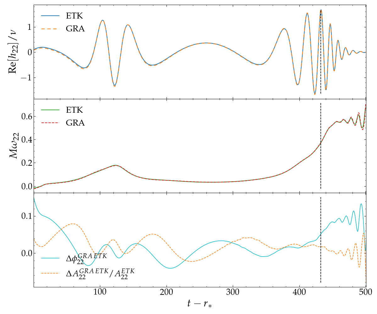
We display the results of our post-processed waveforms for ETK42q1s0,50q1s0 in Fig. 2. We write the modes of the strain in terms of the amplitude and phase as

$$h_{\ell m}(t)=A_{\ell m}(t)e^{i\phi_{\ell m}(t)}$$ (5)

and introduce the difference between EinsteinToolkit and GR-Athena++ results by

$$\Delta A_{22}^{GRA\,ETK} \mathrel{\mathop{\mathchar 58\relax}}=A_{22}^{GRA}-A_{22}^{ETK},$$

$$\Delta\phi_{22}^{GRA\,ETK} \mathrel{\mathop{\mathchar 58\relax}}=\phi_{22}^{GRA}-\phi_{22}^{ETK}$$ (6)

Figure 2: Example orbit, waveforms, frequency, and amplitude and phase difference, for a direct capture (ETK42q1s0, GRA42q1s0, left panel) and zoom-whirl (ETK50q1s0, GRA50q1s0, right panel). The differences are defined in (II.4). We only show the trajectories of one of the black holes to ease visualization. Since these are equal-mass simulations the other trajectory can be obtained by reflection symmetry. In the direct capture case the black holes plunge almost immediately, without completing a full orbital cycle. Therefore, the waveform is dominated by merger and ringdown. Conversely, in the zoom-whirl scenario, the bodies undergo multiple encounters before merging, each close passage corresponds to a GW burst. In our code comparison, there is no alignment applied to the waveforms. We show the merger time as a vertical dashed on bottom panels.

II.5 Energetics

We compute the radiated energy and angular momentum as a function of time, as (see e.g. Damour et al. (2012))

$$\dot{E}=\frac{1}{16\pi}\sum_{(\ell,m)}\dot{h}_{\ell m}\dot{h}_{\ell m}^{*}$$ (7)

$$\dot{J}=\frac{1}{16\pi}\sum_{(\ell,m)}m\Im[h_{\ell m}\dot{h}_{\ell m}^{*}]$$ (8)

Note that here we are formally extrapolating to infinity by using the formula (1). Our data includes modes with $2\leq l\leq 8$ and $m=-\ell\ldots\ell$, so in practice the sums are limited to these values. We have found that the modes $m=0$ are numerically noisy so do not include them in the computation. Integrating the fluxes $\dot{E}$, $\dot{J}$ over time, we obtain the total radiated energy and angular momentum. This allows us to define the energy and angular momentum as a function of time $t$

$${\cal E}(t) =E_{i}^{\rm ADM}-\int_{t}^{\infty}dt^{\prime}\dot{E}(t^{\prime})$$ (9)

$${\cal J}(t) =J_{i}^{\rm ADM}-\int_{t}^{\infty}dt^{\prime}\dot{J}(t^{\prime})$$ (10)

where $E_{i}^{\rm ADM}$, $J_{i}^{\rm ADM}$ are the initial ADM total energy and angular momentum of the system as shown in Table 1. Following Nagar et al. (2016), we define the dimensionless binding energy and dimensionless angular momentum as

$$E_{b}(t) =\frac{{\cal E}(t)-M}{\mu}$$ (11)

$$j(t) =\frac{{\cal J}(t)}{M\mu}$$ (12)

where $M=m_{1}+m_{2}$ is the sum of the individual initial ADM masses and $\mu=m_{1}m_{2}/M$.

Energetics are a meaningful and robust tool to compare NR data to EOB, e.g. Damour et al. (2012); Bernuzzi et al. (2012a, 2014); Nagar et al. (2016). In the case of quasi-circular orbits, the NR initial puncture parameters can be constructed to match the 3PN prediction. When junk radiation is correctly taken into account, the initial evolution drives the binary very close to the EOB curve, that is more bound than the 3PN curve Damour et al. (2012). We observe in our dynamical capture scenario that the initial burst of junk radiation has a smaller impact on the energetics with respect to the quasi-circular case. However, other sources of inaccuracies like residual gauge ambiguities in the determination of the puncture parameters from the EOB energetics and the reconstruction of the strain from $\psi_{4}$ can play a role. Overall, we observe these effects are sufficiently small that the EOB/NR agreement is within the NR errors in the early phase of the dynamics. However, in some cases we allow for a small (less than $1\%$) adjustment in the ADM quantities to obtain EOB waveforms that best match the NR simulations. These corrections are then also employed when we compare the energy curves between EOB and NR.

II.6 Faithfulness

The faithfulness (or match) is a common measure to quantify the global difference between two waveforms. For two signals in the time domain $h_{1}(t)$, $h_{2}(t)$ the match is defined as

$${\cal F}=\frac{\langle h_{1},h_{2}\rangle}{\sqrt{\langle h_{2},h_{2}\rangle\langle h_{1},h_{1}\rangle}}\,,$$ (13)

where the inner product, assuming a noise function $S_{n}(f)$, is defined as

$${\langle h_{1},h_{2}\rangle}=4\Re\int\frac{\tilde{h}_{1}(f)\tilde{h}^{*}_{2}(f)}{S_{n}(f)}df$$ (14)

Here the $\tilde{h}_{1}(f)$ and $\tilde{h}_{2}(f)$ are the Fourier transforms of the time domain waveforms, and the integral covers the frequency interval $Mf\in[0.005,0.1]$ of the signal. In this work we consider a uniform PSD ($S_{n}(f)\equiv 1$) unless explicitly stated. We have checked that the power is concentrated in this interval for all of our simulations. In turn, the unfaithfulness, or mismatch, is given by $\overline{{\cal F}}=1-{\cal F}$. The unfaithfulness, which ranges in [0,1], is equal to the fractional loss of signal-to-noise ratio due to the difference between the two compared waveforms. We compute the matches using the algorithm optimized$\_$match implemented in pyCBC, which efficiently aligns the waveforms optimizing over the differential phases and time shifts.

II.7 Consistency of the numerical results

We discuss the consistency of the results obtained with EinsteinToolkitand GR-Athena++, focusing on simulations ETK42q1s0, 48q1s0, 50q1s0. This will provide error estimates for our NR simulations needed to assess the EOB/NR comparisons later on.

We consider three resolutions, resulting from taking $\delta x=\{3,4,6\}M$ at the coarsest level for EinsteinToolkit and $N_{M}=\{256,192,128\}$ for GR-Athena++, since their corresponding puncture resolutions match. We summarize the relevant technical information for these simulations in Table 2. In the main text, we focus on the amplitude and phase differences for the leading modes $(2,2)$ of the strain, and comment on some other observables in the appendices.

Table 2: [Technical information for simulations ETK42q1s0,48q1s0, 50q1s0 and GRA42q1s0,48q1s0, 50q1s0. We have runs at Low (L), Medium (M), and High (H) resolutions for each case. The quantities shown are: coarsest level resolution for EinsteinToolkit ($\delta x$), number of grid points at the edges of the coarsest level for GR-Athena++ ($N_{M}$), resolution at extraction radius ($\delta x_{R}$), resolution at puncture ($\delta x_{p}$), total simulation time $t_{\rm end}$, and number of CPUs used. The number of points on the spherical grid where extraction is performed is 3200 for EinsteinToolkit simulations and 9002 for GR-Athena++ ($n_{Q}=30$). Note in particular that the puncture resolution $\delta x_{p}$ matches for the corresponding resolutions in each code. All physical quantities are measured in units of $M$.]

ID	res	$\delta x$	$N_{M}$	$\delta x_{R}$	$\delta x_{p}[10^{-2}]$	$t_{\rm end}$	CPUs
	L	6	–	1.5	2.3438	320	180
ETK42q1s0	M	4	–	1.0	1.5625	320	288
	H	3	–	0.75	1.1719	320	288
	L	6	–	1.5	2.3438	450	180
ETK48q1s0	M	4	–	1.0	1.5625	450	288
	H	3	–	0.75	1.1719	450	288
	L	6	–	1.5	2.3438	750	180
ETK50q1s0	M	4	–	1.0	1.5625	750	288
	H	3	–	0.75	1.1719	750	288
	L	–	128	3.0	2.3438	500	768
GRA42q1s0	M	–	192	2.0	1.5625	500	1536
	H	–	256	1.5	1.1719	500	2560
	L	–	128	3.0	2.3438	550	768
GRA48q1s0	M	–	192	2.0	1.5625	550	1536
	H	–	256	1.5	1.1719	550	2560
	L	–	128	3.0	2.3438	800	768
GRA50q1s0	M	–	192	2.0	1.5625	800	1536
	H	–	256	1.5	1.1719	800	2560

II.7.1 Self-convergence

We begin by decomposing the leading modes in amplitude and phase as in (5). We compare these for different resolutions as a function of time, performing time interpolation of third order. Let us denote the amplitudes and phases at a given resolution by $A_{L,M,H}$, $\phi_{L,M,H}$. We can claim convergence of order $r$ if

$$\frac{A_{H}-A_{M}}{A_{L}-A_{M}}\approx SF(r)$$ (15)

where the scaling factor $SF$ is given by

$$SF(r)=\frac{\delta x_{H}^{r}-\delta x_{M}^{r}}{\delta x_{M}^{r}-\delta x_{L}^{r}}$$ (16)

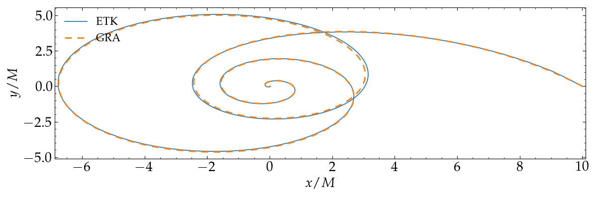
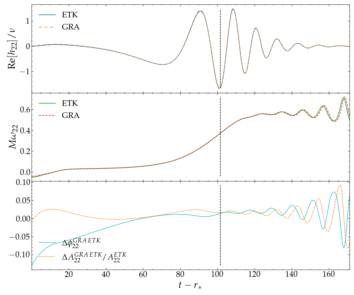
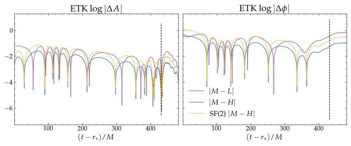
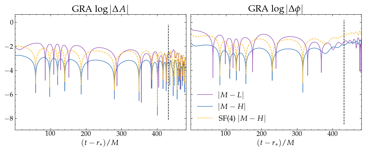
and similarly for the phases, see e.g. Bernuzzi et al. (2012b). Note that the left hand side of (15) is a varying function of time, so that convergence can vary during different stages of the waveform. We show sample results for self-convergence as a function of time for simulations ETK50q1s0 and GRA50q1s0 in Fig. 3. Note that to ease the visualization of the relation (15) we do not normalize the amplitude differences. We record the (normalized) amplitude and phase differences at merger, along with the waveforms mismatches in Table 3.

Our data for ETK50q1s0 is compatible with second-order convergence before merger, while near and after merger the convergence order increases to fourth order. The time-dependent self-convergence results are compatible with the behaviour of the mismatches shown in Table 3, which also decrease with increasing resolution. In the case of GR-Athena++, we observe convergence of order 4 or higher before merger, but after merger the convergence rate for the phase worsens. The mismatches also decrease with increasing resolution.

The self-convergence results for the (normalized) amplitude and phase differences at merger in Table 3 can be taken as a proxy for the accuracy of the NR simulations when comparing to EOB. Roughly speaking, differences between Medium resolution simulations (used for the bulk of our simulations) and High resolution is around $0.1\%$ for the amplitude and of the order of $0.01$ radians for the phases.

Figure 3: Self-convergence for ETK50q1s0 (top row) and for GRA50q1s0 (middle row). Displayed are the differences in amplitude and phase for consecutive resolutions $(L-M)$, $(M-H)$. In addition, we overlay the curves for $SF(r)(M-H)$ which allows us to test for convergence of a given order $r$, see (16), which we show in each panel. Bottom row: comparison between ETK50q1s0 and GRA50q1s0 at fixed resolution. The simulations for $(L,M,H)$ resolutions have the same grid spacing at puncture location, see Table 2. For each case, we display the absolute value of the difference in normalized amplitude and phase for every available resolution.

Table 3: Self-convergence results for the $\ell=m=2$ strain mode for consecutive resolutions for EinsteinToolkit and GR-Athena++ at merger time. From left to right, the columns report: the relative amplitude differences, the phase differences and the unfaithfulness between two consecutive resolutions.

ID	res1,2	$\Delta A^{{\rm res}_{1}-{\rm res}_{2}}_{\rm 22,mrg}/A^{{\rm res}_{1}}_{\rm 22,mrg}$	$\Delta\phi^{{\rm res}_{1}-{\rm res}_{2}}_{\rm 22,mrg}$	$\overline{{\cal F}}$
ETK42q1s0	L,M	$-1.86\cdot 10^{-3}$	$2.265\cdot 10^{-3}$	$7.469\cdot 10^{-6}$
ETK42q1s0	M,H	$-3.29\cdot 10^{-3}$	$-2.95\cdot 10^{-3}$	$1.101\cdot 10^{-4}$
ETK48q1s0	L,M	$-9.73\cdot 10^{-3}$	$-4.55\cdot 10^{-2}$	$2.048\cdot 10^{-4}$
ETK48q1s0	MH	$-3.47\cdot 10^{-3}$	$-2.02\cdot 10^{-2}$	$7.393\cdot 10^{-5}$
ETK50q1s0	L,M	$-1.02\cdot 10^{-3}$	$-3.63\cdot 10^{-1}$	$1.917\cdot 10^{-3}$
ETK50q1s0	M,H	$-1.33\cdot 10^{-5}$	$-5.85\cdot 10^{-2}$	$5.463\cdot 10^{-5}$
GRA42q1s0	L,M	$-1.32\cdot 10^{-3}$	$5.257\cdot 10^{-3}$	$9.756\cdot 10^{-6}$
GRA42q1s0	M,H	$-1.14\cdot 10^{-3}$	$1.715\cdot 10^{-3}$	$1.332\cdot 10^{-6}$
GRA48q1s0	L,M	$-2.74\cdot 10^{-3}$	$1.686\cdot 10^{-2}$	$1.352\cdot 10^{-5}$
GRA48q1s0	M,H	$-2.65\cdot 10^{-4}$	$-8.38\cdot 10^{-3}$	$9.574\cdot 10^{-6}$
GRA50q1s0	L,M	$-6.56\cdot 10^{-3}$	$2.204\cdot 10^{-2}$	$9.405\cdot 10^{-5}$
GRA50q1s0	M,H	$-1.06\cdot 10^{-3}$	$-1.30\cdot 10^{-2}$	$1.484\cdot 10^{-5}$

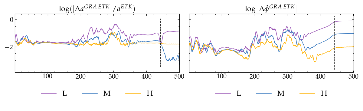
II.7.2 Code comparison

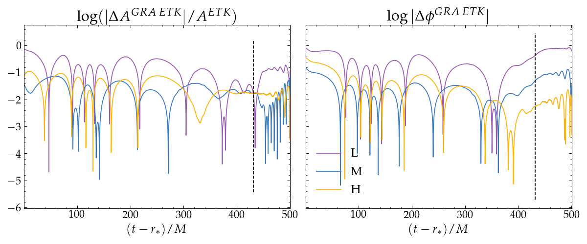
We now focus on the comparison between EinsteinToolkit and GR-Athena++. We display the amplitude and phase differences as a function of time for the leading modes of ETK50q1s0 and GRA50q1s0 at the bottom of Fig. 3. The cases ETK42q1s0, 48q1s0 and GRA42q1s0, 48q1s0 behave similarly. We summarize the information regarding the differences at merger and mismatches in Table 4. For the three simulations, we find that the waveforms are most coincident at Medium resolution. In this case, the amplitude difference at merger is of order $2\%$, being always higher for GR-Athena++. This is compatible with the results of Daszuta et al. (2021) which found a $2\%$ difference at merger with the BAM code Brügmann et al. (2008). While we observe some decrease of the amplitude difference at merger values for High resolution, it is not clear whether they will converge away with increasing resolution further. On the other hand, the phases at merger appear to be converging with increasing resolution, the differences ranging from $10^{-2}$ to $10^{-3}$. At Medium resolution, which is the one used for EinsteinToolkit in the bulk of this work, we find that the differences with GR-Athena++ are roughly of the order of $1\%$ for the amplitude and $0.01$ radians for the phase.

The mismatches for EinsteinToolkit and GR-Athena++ leading modes at Medium resolution are of order $10^{-5}$, and show convergent behaviour for ETK48q1s0, 50q1s0 (GRA48q1s0, 50q1s0) but not for ETK42q1s0 (GRA42q1s0).

We emphasize that the comparisons discussed above involve the leading modes of the extrapolated strain. However, we should keep in mind that the NR results are also affected by our choice of time integration and extrapolation to infinity. We provide a comparison of the raw data by considering the unextrapolated $\psi_{4}$ scalars produced by EinsteinToolkit and GR-Athena++ in Appendix B.1.

Table 4: Comparing the $\ell=m=2$ strain waveform at merger obtained with EinsteinToolkit and GR-Athena++. From left to right, the columns report: the relative amplitude differences, the phase differences at merger and the unfaithfulness for the three configurations simulated with both codes at (L,M,H) resolution.

ID	res	$\Delta A^{\rm GRAETK}_{\rm 22,mrg}/A^{GRA}_{\rm 22,mrg}$	$\Delta\phi^{\rm GRAETK}_{\rm 22,mrg}$	$\overline{{\cal F}}$
	L	$1.640\cdot 10^{-2}$	$1.731\cdot 10^{-2}$	$5.417\cdot 10^{-5}$
42q1s0	M	$1.567\cdot 10^{-2}$	$1.364\cdot 10^{-2}$	$1.788\cdot 10^{-5}$
	H	$1.355\cdot 10^{-2}$	$9.073\cdot 10^{-3}$	$9.145\cdot 10^{-5}$
	L	$2.427\cdot 10^{-2}$	$8.193\cdot 10^{-2}$	$2.216\cdot 10^{-4}$
48q1s0	M	$1.704\cdot 10^{-2}$	$1.973\cdot 10^{-2}$	$1.991\cdot 10^{-5}$
	H	$1.388\cdot 10^{-2}$	$7.851\cdot 10^{-3}$	$1.538\cdot 10^{-5}$
	L	$1.099\cdot 10^{-2}$	$4.363\cdot 10^{-1}$	$2.117\cdot 10^{-3}$
50q1s0	M	$1.737\cdot 10^{-2}$	$5.084\cdot 10^{-2}$	$2.721\cdot 10^{-5}$
	H	$1.848\cdot 10^{-2}$	$5.683\cdot 10^{-3}$	$2.206\cdot 10^{-6}$

III Effective-One-Body model

In this work we will use the eccentric version of the TEOBResumS Nagar et al. (2020); Riemenschneider et al. (2021) effective-one-body (EOB)-based Buonanno and Damour (1999); Buonanno et al. (2006) waveform model, dubbed TEOBResumS-Dalì, as defined in Refs. Nagar et al. (2021b); Bonino et al. (2023). The promotion of the quasi-circular model to the eccentric case follows the idea of Ref. Chiaramello and Nagar (2020) of incorporating non-circular effects in the Newtonian prefactors in both the waveform and radiation reaction. We refer the reader to Ref. Nagar et al. (2021b) and references therein for most of the technical details of the model. Here it is only worth recalling that the EOB description of the merger and ringdown is based on suitable fits of quasi-circular ringdown waveforms Damour and Nagar (2014); Nagar et al. (2020). This approximation looks sufficiently accurate for bound configurations, because the eccentric inspiral has the time to progressively circularize towards merger Nagar et al. (2021b). By contrast, for dynamical capture configurations this is not the case and the quasi-circular ringdown can be inaccurate Albanesi et al. (2021); Gamba et al. (2022). For this reason, one of the final goals of this paper is to show how to use our new NR simulations to suitably improve the model during merger and ringdown. Before discussing this, let us recall that any EOB model essentially depends on two sets of parameters that are informed by NR simulations: (i) one the one hand there are those that directly appear in the dynamics, i.e. as effective modifications to the EOB Hamiltonian. Belonging to this class are the effective 5PN parameter $a_{6}^{c}$ entering the $A$ potential of TEOBResumSor the effective next-to-next-to-next-to-leading order parameter $c_{3}$ used to improve the corresponding spin-orbit coupling); (ii) on the other hand, there are parameters used to improve the shape of the waveform during plunge up to merger via the next-to-quasi-circular (NQC) correction or to accurately describe the postmerger-ringdown signal. In this paper we do not focus on exploring the effect of the dynamical parameters, the values of which we set to those determined in Nagar et al. (2021b), but rather explore the impact of informing the remaining ones using data from our dynamical capture BBH simulations. In particular, we want to: (i) obtain new, NR-informed, next-to-quasi-circular corrections to the waveform and (ii)use a new NR-informed merger and ringdown model. Since our NR simulations cover parameter space in a sparse way, we can only use the NR information separately for each datasets, and cannot present global fits of the NR-informed parameters designed to cover the full parameter space. We therefore aim to illustrate what is needed to improve the current model for hyperbolic capture and quantify the improvement, leaving the development of global fits for future work. From now on, we will focus only on the quadrupole waveform for simplicity, although the same approach could be extended to the other multipoles. We decompose it in amplitude and phase as

$$h_{22}=A_{22}e^{-i\phi_{22}}\ ,$$ (17)

where both $(A_{22},\phi_{22})$ are functions of time $t$. The waveform frequency is $\omega_{22}\equiv\dot{\phi}_{22}$. In addition, we will use the $\nu$-normalized waveform amplitude $\hat{A}_{22}\equiv A_{22}/\nu$. Following the standard TEOBResumS procedure for quasi-circular binaries Nagar et al. (2020); Riemenschneider et al. (2021), we count four parameters related to NQC corrections and seven parameters needed to model the postmerger-ringdown part of the waveform. In practice, one needs to extract eleven numbers from each NR simulation. The NR-informed parameters are:

• The four NQC parameters $(a^{22}_{1},a^{22}_{2},b^{22}_{1},b^{22}_{2})$ that enter the NQC waveform correction

  $$\hat{h}_{22}^{\rm NQC}=(1+a_{1}^{22}n^{22}_{1}+a_{2}^{22}n^{22}_{2})e^{{\rm i}(b_{1}n^{22}_{3}+b_{2}n^{22}_{4})}\ .$$ (18)

  Here, the functions $n_{i}^{22}$ define the NQC basis (see in particular text around Eq. (13) of Ref. Nagar et al. (2021b)), are determined by imposing continuity between the EOB waveform and the NR amplitude and frequency values $(\hat{A}^{\rm NR}_{\rm NQC},\dot{\hat{A}}^{\rm NR}_{\rm NQC},\omega^{\rm NR}_{\rm NQC},\dot{\omega}^{\rm NR}_{\rm NQC})$ evaluated at the NQC extraction time $t_{\rm NQC}^{\rm NR}$. For each mode, $t_{\rm NQC}^{\rm NR}=t^{\rm NR}_{\rm A^{\rm max}}+2M$, where $t^{\rm NR}_{\rm A^{\rm max}}$ is the location of the amplitude’s peak.

• The five parameters entering the ringdown template as introduced in Ref. Damour and Nagar (2014)

  $$\theta^{\rm RD}=(\hat{A}_{\rm max},\omega_{\rm max},c_{3}^{A},c^{3}_{\phi},c^{4}_{\phi})\,.$$ (19)

  The values of the amplitude and frequency at amplitude maximum $(A_{\rm max},\omega_{\rm max})$ are directly read from the NR waveform. By contrast, the parameters $(c_{3}^{A},c^{3}_{\phi},c^{4}_{\phi})$ are obtained by fitting the postmerger-ringdown waveform following Damour and Nagar (2014).

• The postmerger template also depends on the (complex) frequency of the first two quasi-normal-modes that are determined from the mass and dimensionless spin of the final black hole $(M_{f},\hat{a}_{f})$ interpolating the tables of Ref. Berti et al. (2006).

Table 5 lists all the NR-informed parameter for each NR dataset considered. The last two columns also report the EOB/NR difference in the binding energy at merger and the phase difference $\Delta\phi^{\rm EOBNR}_{22}\equiv\phi^{\rm EOB}_{22}-\phi^{\rm NR}_{22}$. Note that the latter is computed, as we will see below, using an improved model with the NR-informed ringdown for each dataset. The origin of these numbers will be discussed in detail in Sec. IV below.

Figure 4: Relation between NR initial data and EOB ones for two selected configurations. The procedure of tuning phenomenological corrections to $(E_{0}^{\rm ADM},J_{0}^{\rm ADM})$ using Eqs. (20)-(21) is globally more efficient (especially for the ETK48q1s0 dataset) than the straightforward transformation from ADM to EOB coordinates.

Table 5: Informing the EOB model with NR data. From left to right the columns report: the name of the dataset, the $\nu$-normalized quadrupole waveform amplitude at merger time $\hat{A}_{22}^{\rm max}=A_{22}^{\rm max}/\nu$ and the corresponding frequency; the mass $M_{f}$ and dimensionless angular momentum $\hat{a}_{f}\equiv J_{f}/M_{f}^{2}$ of the final remnant black hole; the NR values used to determine the NQC corrections; the NR-informed parameters of the postmerger fit. The last two columns report the EOBNR difference in the binding energy per reduced mass at merger $\delta E_{\rm b,\,mrg}^{\rm EOBNR}\equiv E_{\rm b,mrg}^{\rm EOB}-E_{\rm b,mrg}^{\rm NR}$ and the corresponding phase difference at merger obtained using the NR-informed upgraded model.

#	ID	$\hat{A}^{\rm max}_{22}$	$\omega^{\rm max}_{22}$	$M_{f}$	$a_{f}$	$\hat{A}^{\rm NQC}_{\rm NR}$	$\dot{\hat{A}}_{\rm NR}^{\rm NQC}$	$\omega^{\rm NQC}_{\rm NR}$	$\dot{\omega}^{\rm NQC}_{\rm NR}$	$c_{3}^{A}$	$c_{3}^{\phi}$	$c_{4}^{\phi}$	$\tilde{\delta}E_{\rm b,mrg}$	$\Delta\phi^{\rm EOBNR}_{22,\rm mrg}$[rad]
1	ETK37q1s0	$1.419$	$0.335$	$0.978$	$0.685$	$1.399$	$-0.020$	$0.369$	$0.017$	$-0.016$	$1.74076$	$0.39046$	$+0.0045$	$-0.003$
2	ETK42q1s0	$1.675$	$0.370$	$0.965$	$0.725$	$1.659$	$-0.016$	$0.398$	$0.014$	$-0.187$	$2.48789$	$0.73609$	$+0.0038$	$-0.008$
3	ETK44q1s0	$1.768$	$0.388$	$0.958$	$0.728$	$1.754$	$-0.015$	$0.410$	$0.011$	$-0.243$	$3.24197$	$1.19834$	$+0.0039$	$-0.029$
4	ETK46q1s0	$1.821$	$0.377$	$0.949$	$0.716$	$1.814$	$-0.007$	$0.394$	$0.009$	$-0.510$	$5.30479$	$1.33265$	$+0.0025$	$-0.015$
5	ETK48q1s0	$1.518$	$0.346$	$0.950$	$0.675$	$1.509$	$-0.010$	$0.370$	$0.012$	$-0.422$	$4.42020$	$1.91359$	$+0.0030$	$-0.096$
6	ETK50q1s0	$1.679$	$0.364$	$0.949$	$0.697$	$1.671$	$-0.008$	$0.383$	$0.010$	$-0.477$	$4.80545$	$1.26372$	$+0.0033$	$-0.011$
7	ETK42q1s050--	$1.429$	$0.307$	$0.981$	$0.515$	$1.409$	$-0.020$	$0.336$	$0.014$	$0.001$	$1.59410$	$0.28785$	$+0.0041$	$-0.030$
8	ETK42q1s025--	$1.522$	$0.338$	$0.976$	$0.626$	$1.506$	$-0.017$	$0.367$	$0.014$	$-0.072$	$2.07120$	$0.53770$	$+0.0040$	$-0.012$
9	ETK42q1s025++	$1.863$	$0.403$	$0.943$	$0.793$	$1.849$	$-0.015$	$0.425$	$0.012$	$-0.459$	$5.39366$	$2.68358$	$+0.0025$	$-0.035$
10	ETK42q1s050++	$1.487$	$0.428$	$0.940$	$0.832$	$1.476$	$-0.012$	$0.453$	$0.013$	$-0.093$	$2.87101$	$1.14302$	$+0.0057$	$0.014$
11	ETK42q1s050+-	$1.676$	$0.370$	$0.965$	$0.724$	$1.660$	$-0.017$	$0.398$	$0.014$	$-0.181$	$2.49269$	$0.73682$	$+0.0038$	$-0.012$
12	ETK42q1.5s0	$1.763$	$0.374$	$0.962$	$0.707$	$1.748$	$-0.015$	$0.398$	$0.012$	$-0.297$	$3.17798$	$1.12475$	$+0.0029$	$-0.003$
13	ETK42q2s0	$1.734$	$0.327$	$0.957$	$0.633$	$1.730$	$-0.004$	$0.338$	$0.006$	$-0.845$	$9.62619$	$1.39233$	$-0.0003$	$-0.026$
14	ETK42q2.15s0	$1.681$	$0.337$	$0.963$	$0.630$	$1.674$	$-0.007$	$0.358$	$0.011$	$-0.597$	$-0.00004$	$0.00001$	$+0.0030$	$+0.032$

Figure 5: Equal-mass, nonspinning case. EOB/NR waveform comparison. Top panels: $\ell=m=2$ real part and frequency evolution for ETK42q1s0 (left) and ETK50q1s0 (right). Bottom panels: EOB/NR phase and (relative) amplitude differences obtained by increasing progressively the amount of NR input to describe the merger and ringdown part.

III.1 Connecting NR initial data with EOB ones

In order to compare our results from NR and EOB, we need to specify which parameters shall we input in TEOBResumS based on the initial NR data. Initial data for dynamical capture in TEOBResumS are given by fixing the mass ratio $q$, initial energy $E_{\rm EOB}/M$, dimensionless initial orbital angular momentum $p_{\varphi}=L^{\rm EOB}/(\mu M)$, dimensionless spins $\chi_{1,2}^{\rm EOB}\equiv S_{i}/m_{i}^{2}$ and initial separation $r_{\rm EOB}$. In practice, the initial EOB parameters are obtained by identifying the NR and EOB spin values, i.e. $\chi_{1,2}^{\rm EOB}=\chi_{1,2}^{\rm NR}$, and matching the other dynamical quantities to the initial ADM values from NR simulations as

$$E_{\rm EOB} =E_{0}^{\rm ADM}+\Delta E_{\rm EOB}\ ,$$ (20)

$$L_{\rm EOB} =J_{0}^{\rm ADM}-(S_{1}+S_{2})+\Delta J_{\rm EOB}\ ,$$ (21)

$$r_{\rm EOB} =D+\Delta r_{\rm EOB}\ ,$$ (22)

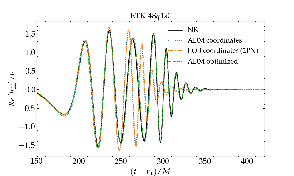
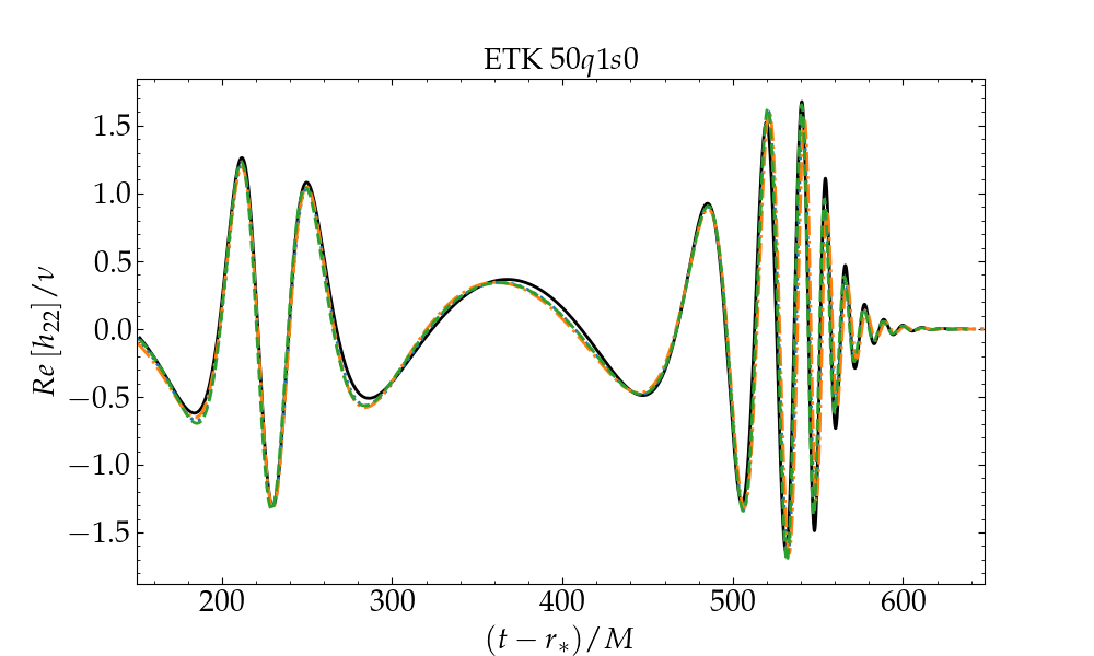
where $(\Delta E_{\rm EOB},\Delta J_{\rm EOB},\Delta r_{\rm EOB})$ are arbitrary corrections to the NR quantities to be determined as follows. We choose the initial EOB distance $\Delta r_{\rm EOB}$ such that the EOB waveforms extend to earlier times at least as much as the NR simulations. For this reason, we choose $\Delta r_{\rm EOB}=4M$. Following Gamba et al. (2022), values of $(\Delta E_{\rm EOB},\Delta J_{\rm EOB})$ are chosen by minimizing the EOB/NR mismatch. More precisely, when performing this minimization we consider both the ring-down and NQC information in the EOB waveform. We implement this using the algorithm dual_annealing from the scipy Python library Virtanen et al. (2020). We find that we obtain a good match for the signal length considering $|\Delta E_{\rm EOB}|<0.0007E_{\rm ADM}$, $|\Delta J_{\rm EOB}|<0.006J_{\rm ADM}$, see Table 1.

Although this method is efficient and successful, we have to remind the reader that at a rigorous mathematical level the initial puncture parameters expressed in ADM coordinates (relative separation and momenta) should be connected to the corresponding EOB ones by using the corresponding canonical transformation. This was originally obtained in Ref. Buonanno and Damour (1999) at 2PN accuracy. One of the use of this transformation, already suggested in Ref. Buonanno and Damour (1999) was to provide small-eccentricity initial data for NR simulations. This idea was eventually implemented in Ref. Walther et al. (2009) at 3PN accuracy. For completeness, here we also explored this route by converting the ADM quantities $(\vec{P}^{\rm ADM},D)$ to EOB ones $(E_{\rm EOB},p_{\varphi}^{\rm EOB},r_{\rm EOB})$ using the canonical transformation at 2PN. Figure 4 focuses on two datasets, ETK48q1s0 and ETK50q1s0: the NR waveforms (black) are compared with EOB waveforms obtained with different choices of initial conditions. We note that the impact of the optimization and of the canonical transformation (that typically is rather small) depend on the configuration. For ETK48q1s0 the effect of the ADM/EOB canonical transformation is practically negligible, while the phenomenological optimization is more efficient in obtaining the correct initial data. By contrast, for ETK50q1s0 the various choices are practically equivalent.

Figure 6: Unequal-mass ($q=2.15$), nonspinninga case, dataset ETK42q215: EOB/NR phasing comparison including the available higher harmonics. Note that the $(2,2)$ mode is completed by the NR-informed, noncircular, merger and ringdown, while the higher harmonics still retain the standard quasi-circular contributions. Despite this, the agreement is acceptable. Also note some unphysical features in the ringdown for $(4,4)$ and $(5,5)$ due to the calculation of the strain from $\psi_{4}$.

Figure 7: EOB/NR unfaithfulness for the $\ell=m=2$ mode obtained in zero noise for all configurations considered. Note how $\bar{\cal F}$ decreases due to the NR-improvement of the merger and ringdown part of the EOB waveform.

Figure 8: EOB/NR unfaithfulness for the $\ell=m=2$ mode obtained with the zero-detuned, high-power noise spectral density of Advanced LIGO aLI .

Figure 9: EOB/NR comparisons for spin-aligned binaries. Top row: ETK42q1s* configurations with $\chi_{1}=\chi_{2}=0$ (left) and $\chi_{1}=-\chi_{2}=0.5$ (right). The cancelation of the spin-orbit interaction as predicted by the EOB model, is present also in the NR data. Bottom panels: $\chi_{1}=\chi_{2}=-0.5$ (left) and $\chi_{1}=\chi_{2}=+0.5$ (right). When spins are negative, the plunge occurs faster and the signal is shorter than the $\chi_{1}=\chi_{2}=0$ case. When spins are positive, the repulsive character of the spin-orbit coupling yields a first encounter followed then by the plunge and merger. The phase differences are reported in Fig. 10.

IV EOB/NR comparisons

Let us finally focus on the bulk of our results about direct comparisons between EOB and NR waveforms. As usual, we provide two different metrics: (i) phase and amplitude differences in the time domain; (ii) EOB/NR unfaithfulness as defined from Eq. (13) above. In addition, we will also discuss comparisons between the EOB and NR dynamics, as expressed using the gauge-invariant relation between energy and angular momentum.

IV.1 Time-domain phasing and unfaithfulness

The EOB/NR amplitude and phase differences are defined

$$\Delta A^{\rm EOBNR}_{22}\equiv A^{\rm EOB}_{22}-A^{\rm NR}_{22}\ ,$$ (23)

$$\Delta\phi^{\rm EOBNR}\equiv\phi^{\rm EOB}_{22}-\phi^{\rm NR}_{22}\ ,$$ (24)

and are computed once the two waveforms are aligned after fixing an arbitrary time and phase shifts $(\tau,\alpha)$. This is done by minimizing the unfaithfulness (in zero noise) as defined from Eq. (13) above, computed using the algorithm optimized_match of the pyCBC library Nitz et al. (2022).

IV.1.1 Nonspinning configurations

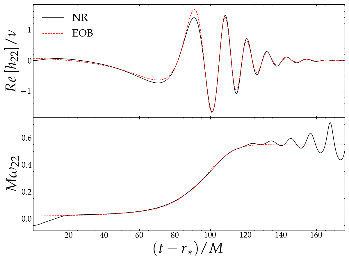
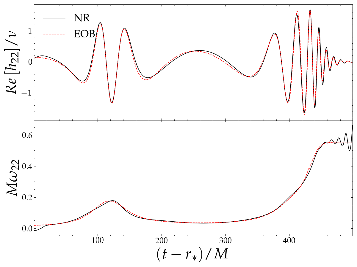
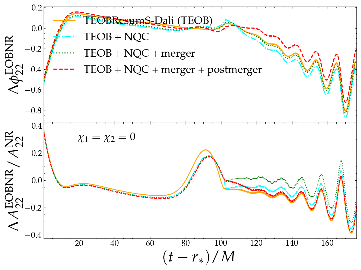
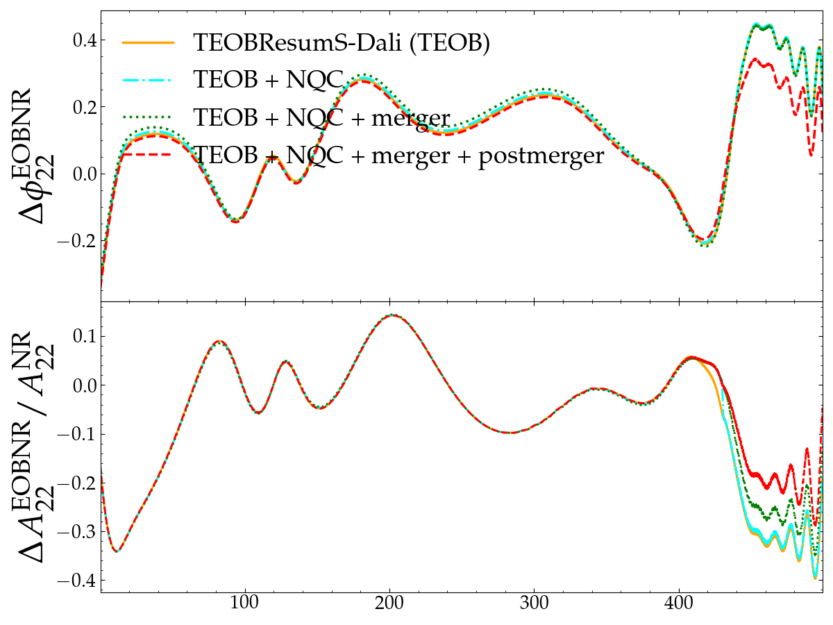
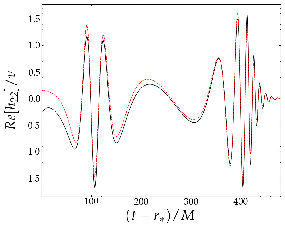
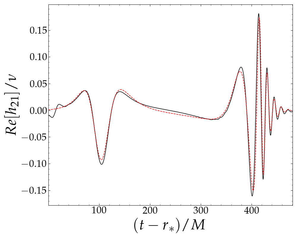
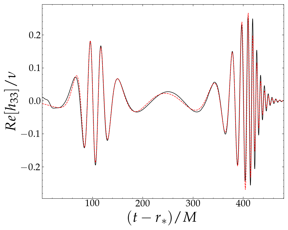
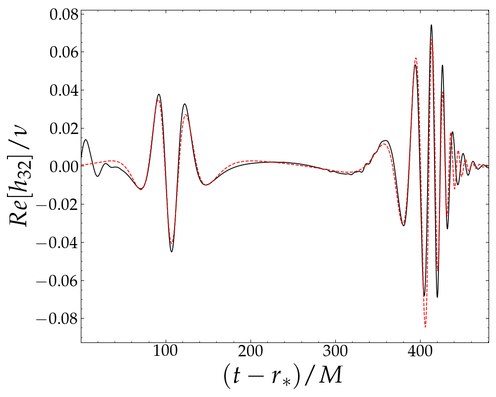
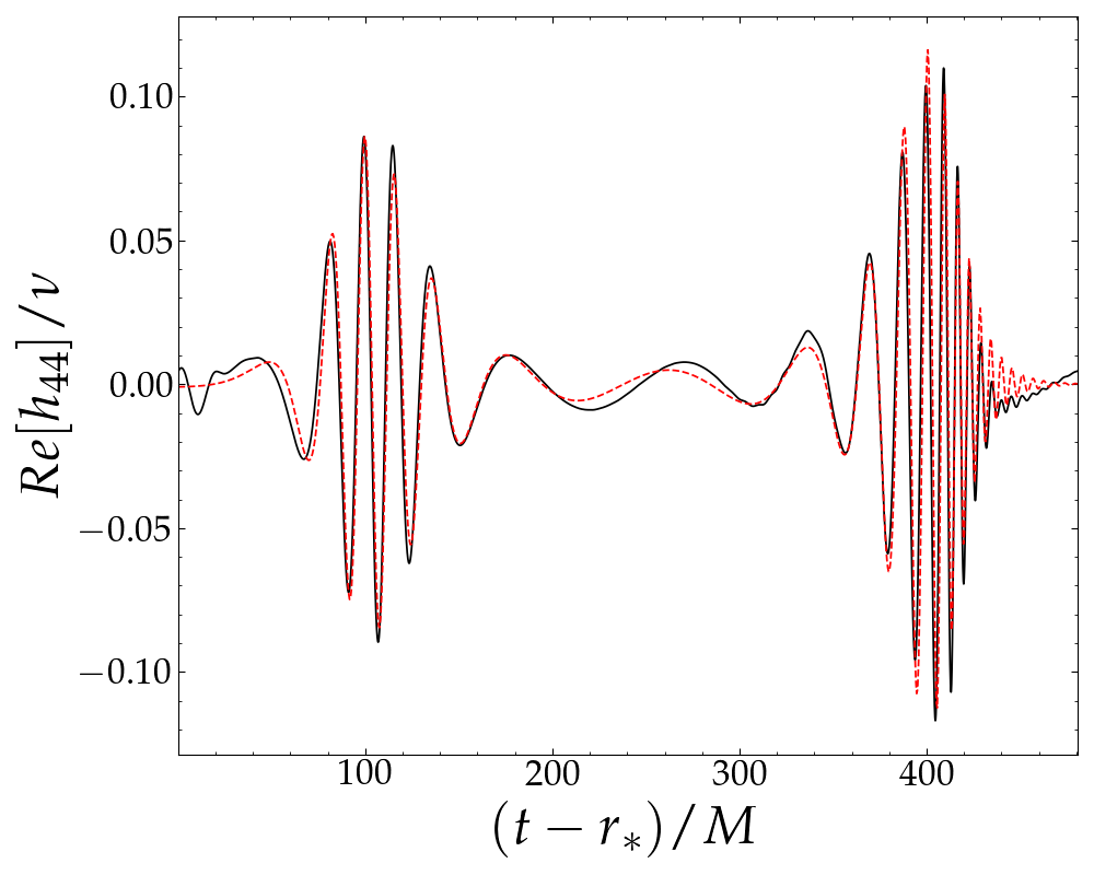
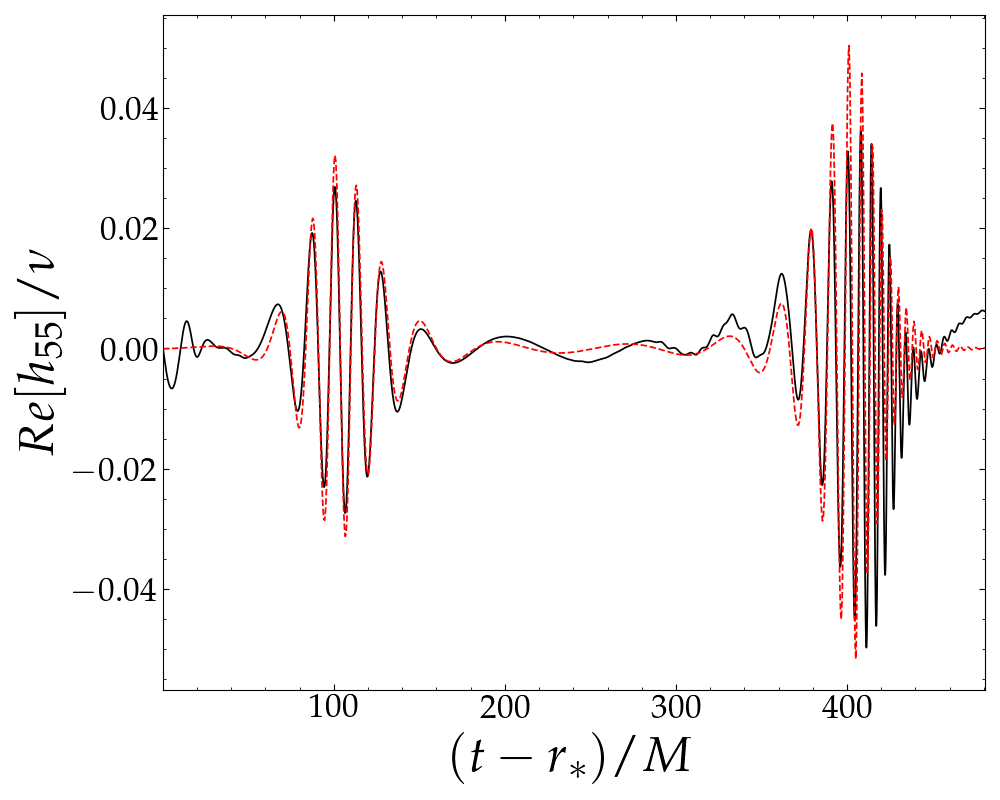
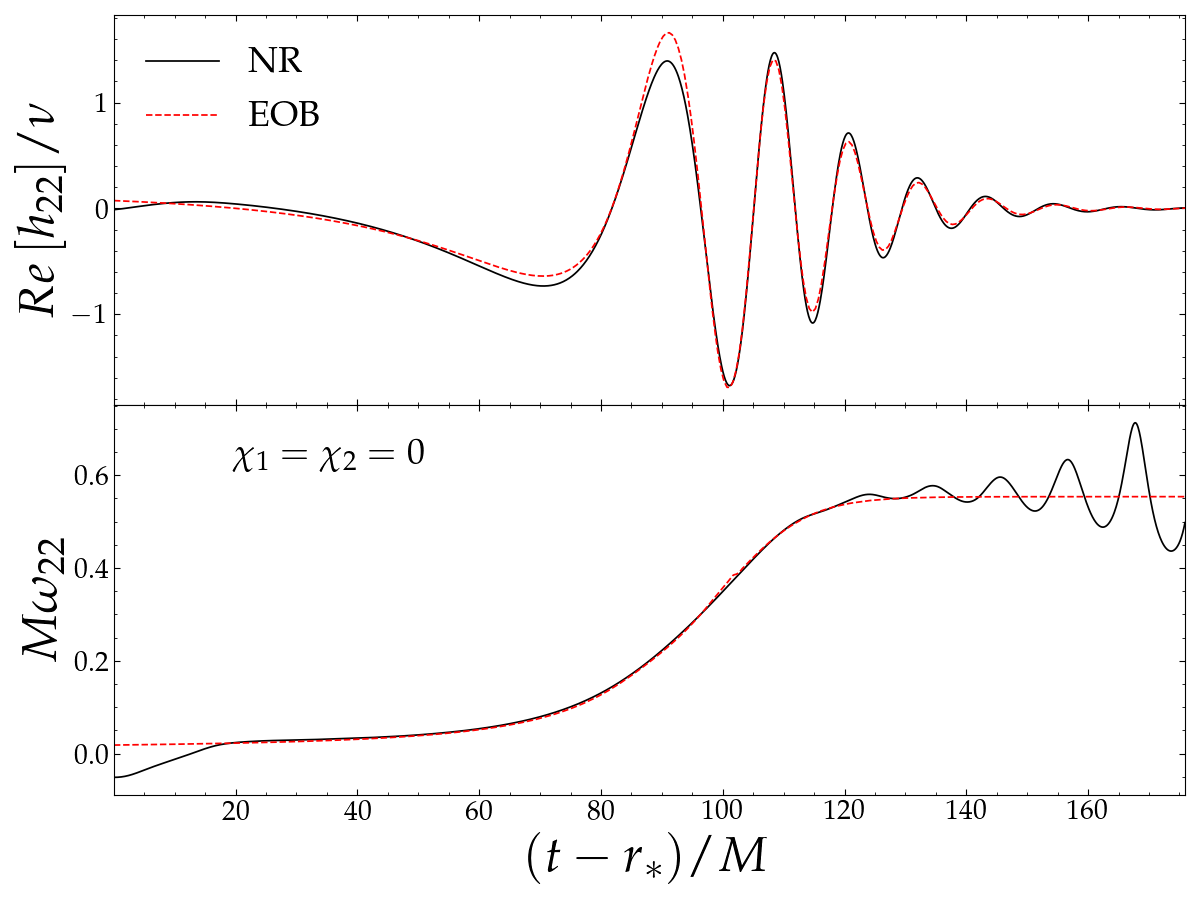
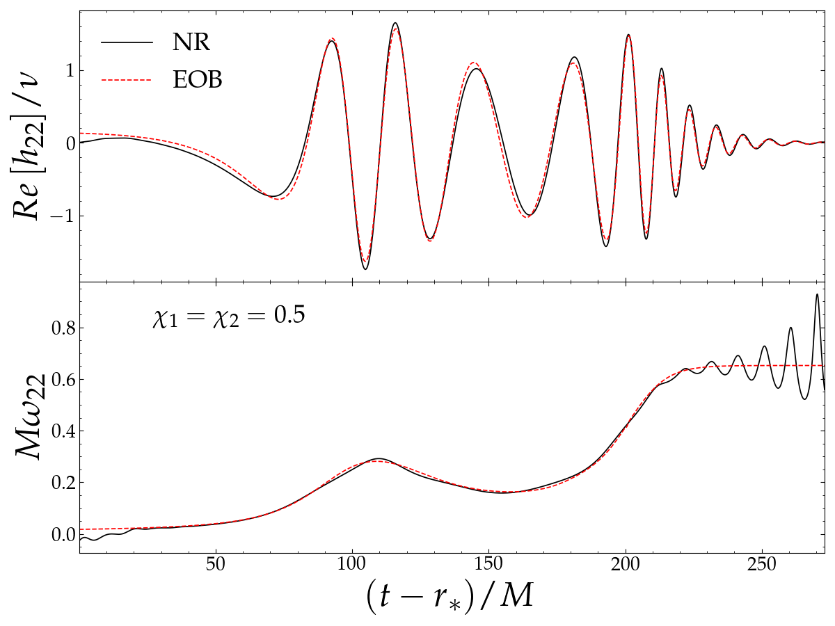
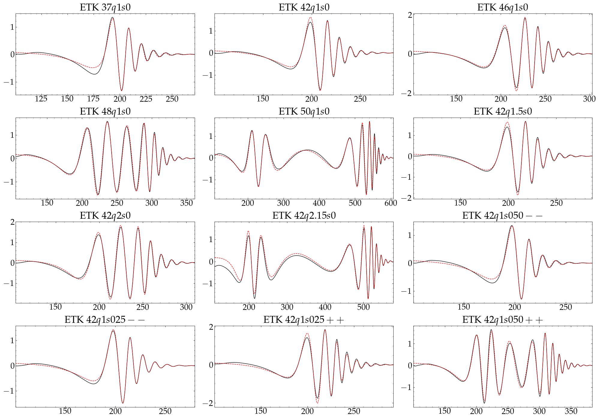
Let us discuss first nonspinning configurations, i.e. datasets from ETK31q1s0 to ETK50q1s0 (equal-mass) and ETK42q1.5s0 to ETK42q2.15s0 (unequal-mass). Focusing first on equal-mass case binaries, the phenomenology changes from a direct capture, ETK31q1s0, to a double encounter, ETK50q1s0. The corresponding EOB/NR time-domain phasing comparisons are shown in Fig. 5. The top panels show the real part of the waveform and the instantaneous gravitational wave frequency, as obtained using the full NQC and ringdown improved model. The bottom panels exhibit the phase difference and the relative amplitude differences obtained with four different versions of the waveform:(i) the standard, TEOBResumSDalì one with the native ringdown informed by quasi-circular information;(ii) the model with NR-informed NQC corrections;(iii) the model with NR-informed NQC corrections and NR-informed merger values of $(\hat{A}_{\rm max},\omega_{\rm max})$; (iv)the full improved model corresponding at the top panel, completed by the NR-informed complete postmerger waveform. The phase differences at merger corresponding to case (iv) above are listed in Table 5. The bottom panels of Fig. 5 indicate that the NR-information injected in the merger-ringdown description may bring a reduction of the order of $\sim 0.1$ rad of the phase difference during the final phases of the coalescence. The differences during either the precursor (for ETK31q1s0) or the first encounter (for ETK50q1s0) are of the order of $0.1$ rad, with trends that suggest that some additional analytic improvement, either in the dynamics or in the waveform Albanesi et al. (2022b), might be needed to reach the NR accuracy level. Despite this, the corresponding values of the EOB/NR unfaithfulness $\bar{F}$ are more than acceptable, as we will see below. Before presenting this calculation, let us focus on the few, nonspinning, dataset with $q\neq 1$. The purpose of this choice was to reliably extract from NR also higher waveform modes and use them to test the corresponding EOB multipoles, tested so far only for eccentric inspirals Nagar et al. (2021b). This is done in Fig. 6, which shows the complete EOB/NR comparison for modes $\{(2,2),(2,1),(3,3),(3,2),(4,4),(5,5)\}$ for the dataset ETK42q2.15s0 with $q=2.15$. For this specific comparison we are using the standard TEOBResumSDalì model without NR-information also in the $(2,2)$ mode. Visually, the EOB/NR agreement is acceptable and can be evidently improved further by injecting NR information. Figure 6 also highlights inaccuracies in the recovering of the strain from $\psi_{4}$ from higher modes, as it is evident from the trend of the post-merger waveform ffor modes $(4,4)$ and $(5,5)$.

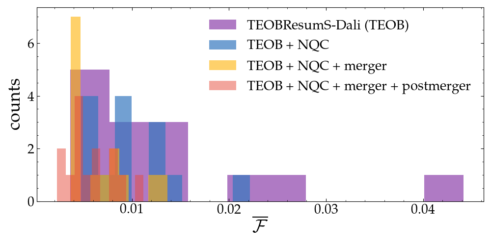
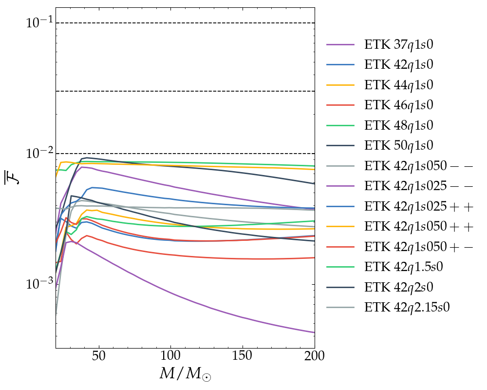
The time-domain phasing analysis is complemented by the calculation of the unfaithfulness $\bar{\cal F}$. This is done either assuming zero noise, $S_{n}(f)=1$, or using the zero-detuned, high power spectral density (PSD) design sensitivity of Advanced Ligo aLI . As it is standard for quasi-circular binaries, this yields $\bar{\cal F}$ as function of the total mass. Assuming $S_{n}(f)=1$, we explore how the increase of NR information used to correctly shape the merger-ringdown part of the waveform reflects on $\bar{F}$. The result of this analysis is found in Fig. 7. The values corresponding to the complete model are also listed in the last column of Table 1. Note that the mismatches are highest for the smallest angular momenta simulation (corresponding to lowest scattering angle ETK37q1s0 and anti-aligned spins ETK42q1s050+-, a dataset to be discussed below). In all other cases, the mismatches are below $1\%$, always obtained after the NR-information procedure. The calculation using the Advanced LIGO PSD is exhibited in Fig. 7 for total mass $20M_{\odot}\leq M\leq 200M_{\odot}$. It is remarkable to note that, despite the absence of any additional tuning on the actual dynamics of the binary (that was informed using only quasi-circular simulations), one has $\bar{\cal F}^{\max}\sim 1\%$ all over the considered configurations.

IV.1.2 Spin

We also considered a few datasets with spin aligned (or anti-aligned) with the orbital angular momentum. Before discussing their properties and putting them in relation with the EOB model, let us recall a pure EOB prediction presented in Ref. Nagar et al. (2021a). The effect of the BH spins (aligned or anti-aligned with the orbital angular momentum) for dynamical capture BBHs was analyzed in Sec. IIIA of Ref. Nagar et al. (2021a). The spin-orbit interaction implemented within the EOB model allowed for a very precise prediction for a $q=1$ dynamical encounter of the changes in the waveform phenomenology with respect to the corresponding nonspinnig case.

Figure 10: EOB/NR phase differences for the configurations of Fig. 9. The markers indicates the location of the waveform amplitude peak. Note the rather small differences (only during the precursor phase) between the $\chi_{1}=\chi_{2}=0$ and $\chi_{1}=-\chi_{2}=0.5$ datasets.

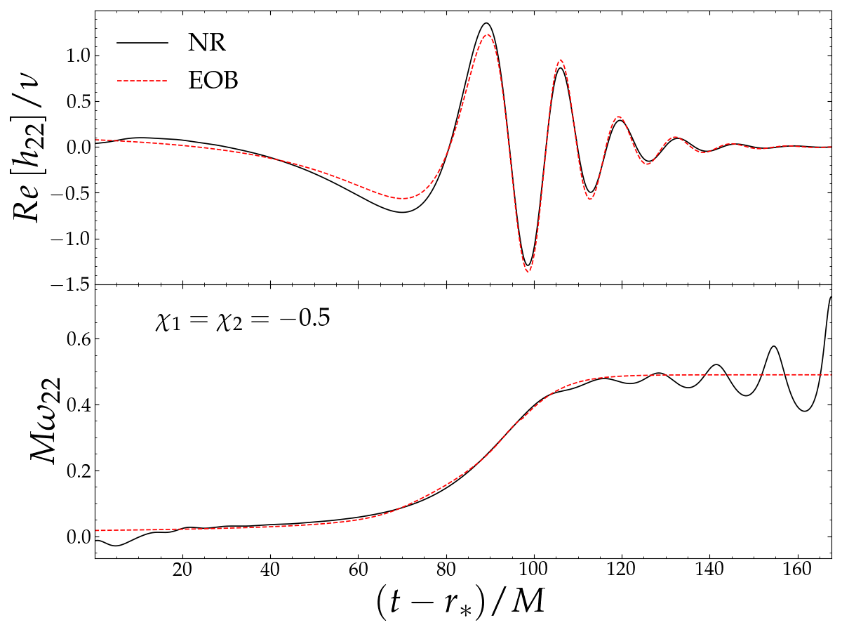
More precisely: (i) if spins are both aligned with angular momentum, the repulsive character of the interaction is such that a configuration that merge in absence of spins can just scatter; (ii) if spins are both anti-aligned with the angular momentum, the attractive character of the spin-orbit interaction entails the plunge to occur on a shorter time scale; (iii) if spins are one aligned and one anti-aligned with the orbital angular momentum the spin-orbit interaction cancels out and the corresponding waveform is substantially equivalent to the nonspinning one. This phenomenology is summarized in Fig. 6 of Ref. Nagar et al. (2021a). Here, we start from the nonspinning configuration ETK42q1s0 and add spins, with dimensionless magnitude $|\chi|=0.25$ and $|\chi|=0.5$ and different orientations. In this second case, we consider the three possible configurations, $\chi_{1}=\chi_{2}=+0.5$, $\chi_{1}=\chi_{2}=-0.5$ ad $\chi_{1}=-\chi_{2}=+0.5$ so to test the analytical prediction of Ref. Nagar et al. (2021a) discussed above. Also here, as it was the case before, it is intended that the EOB waveform for each configuration is completed by the NR-informed NQC corrections and ringdown.

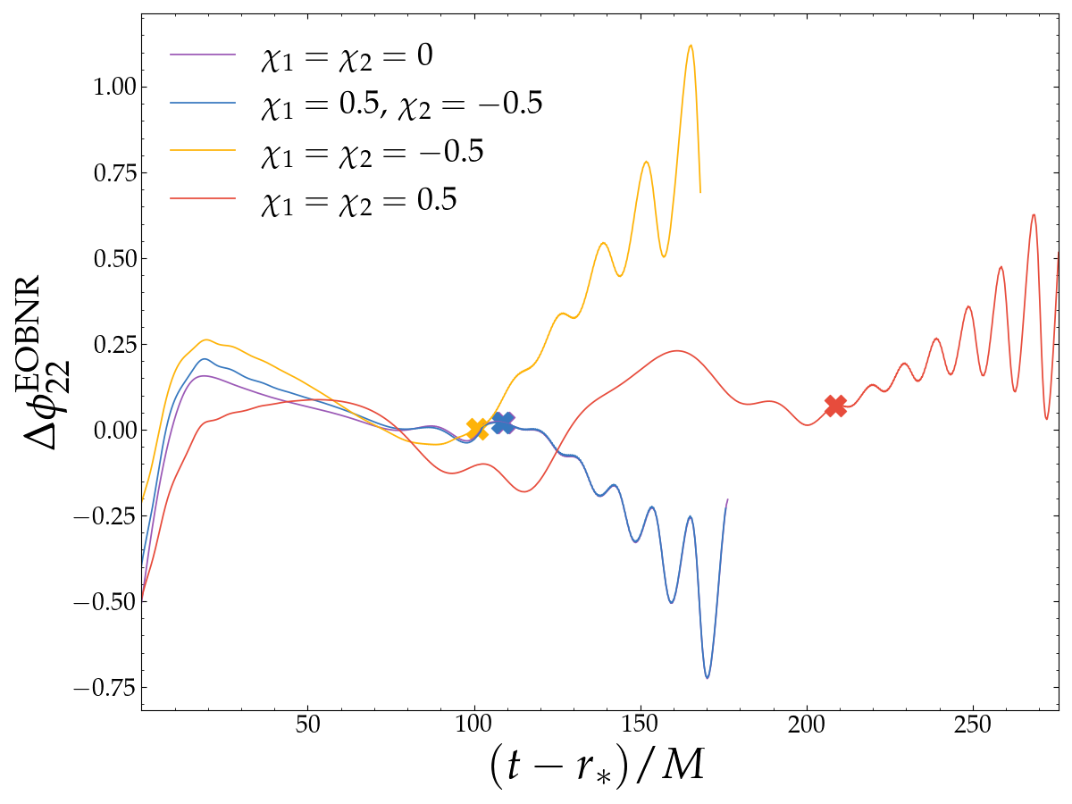
The first row of Fig. 9 displays the nonspinning simulation (left panel) and the one with misaligned spins (right panel). Both NR datasets are also compared with the corresponding EOB waveform (completed by the NR-informed description of merger and ringdown). We see that the analytical prediction of Ref. Nagar et al. (2021a) is fully confirmed, with just very small differences between the waveforms due to spin-spin effects. The bottom row of the picture shows the case with both spins negative (left panel) and positive (right panel). In this second case, we see how the repulsive character of the spin-orbit interaction yields a first encounter (highlighted by the presence of a local maximum in the gravitational wave frequency) then followed by the merger. The actual EOB/NR phase differences are quantified in Fig. 10, which depicts together $\Delta\phi^{\rm EOBNR}_{22}$ for the four datasets.

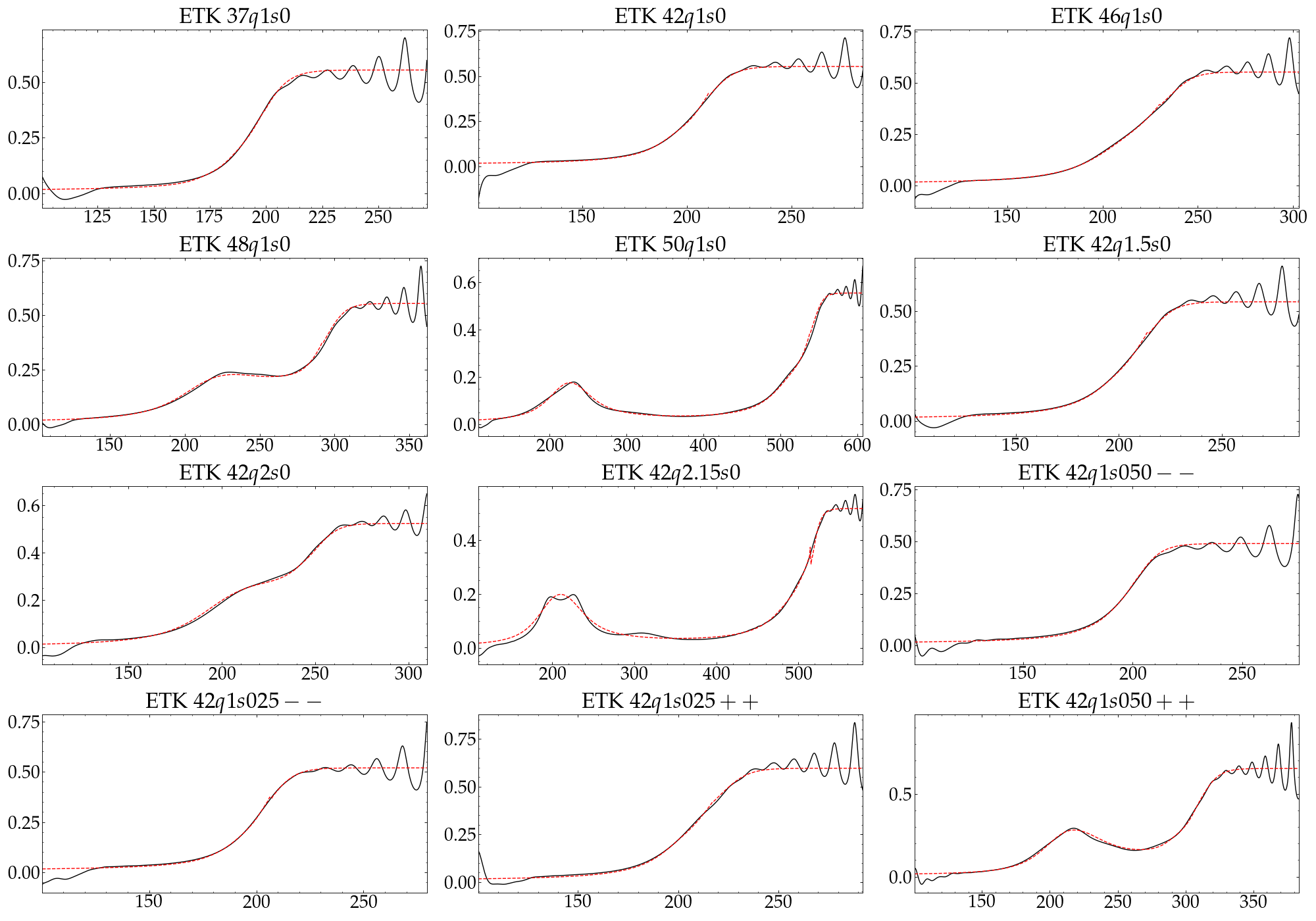
IV.2 Dynamics

We also compared the EOB and NR dynamics expressed using the gauge-invariant relation between energy and angular momentum Damour et al. (2012); Nagar et al. (2016). On the NR side, this quantity can be extracted as the parametric curves $(j(t),E_{b}(t))$ given by Eq. (11) for $t>t_{{\rm junk}}$. On the EOB side, this is just obtained from the evolution of the Hamiltonain dynamics. Note in this respect that it is not computed from the waveform multipoles as in the NR case. We gather the plots for all simulations in Appendix C, and list in Table 5 as meaningful values only the differences at merger. It is interesting to note that EOB/NR differences decrease monotonically with all physical parameters $J_{i}$, $q$, and $\chi$, i.e. as the signals become longer and thus closer to the quasi-circular simulations used to inform the model.

V Conclusions

We have presented new NR simulations of dynamical capture black hole binaries. Our set of simulations includes some of the configurations of Gold and Brügmann Gold and Brügmann (2013) (see also East et al. (2013)), improving the systematic exploration of aligned spins and mass ratio effects. The runs were mostly done using the EinsteinToolkit NR code. A few configurations were also simulated using the GR-Athena++ code for mutual cross checking. The NR strain waveforms (computed here for the first time) are first compared with the state-of-the-art eccentric model TEOBResumS and additionally used to inform it to obtain improved accuracy for merger and ringdown. Our results on the NR side can be summarized as follows:

• We have systematically analyzed configurations with spins. We found that the analytical EOB predictions due to spin-orbit interaction of Ref. Nagar et al. (2021a) in spin-aligned encounters (see Fig.  9) are fully confirmed by NR simulations. More precisely: if the spins are positive, the system has more GW cycles before merger than in the nonspinning case (repulsive character of spin-orbit interaction); if the spins are both negative, the plunge occurs faster with less cycles (attractive character of spin-orbit interaction); when the spins are misaligned and equal (one positive and one negative) the dynamics and waveforms are fully compatible with the nonspinning case.

• We presented the first direct comparisons between EinsteinToolkit and GR-Athena++, corresponding to three different nonspinning equal-mass dynamical captures, previously studied in Ref. Gold and Brügmann (2013). The comparison between the codes shows good quantitative agreement (Sec. II.7.2), and the independent codes display self-convergence (Sec.  II.7.1).

• We have systematically computed the strain waveform (that was absent in Ref. Gold and Brügmann (2013)) for both EinsteinToolkit and GR-Athena++, increasing the amount of currently known information (see in particular the supplementary material of Ref. Gamba et al. (2022), where 3 more configurations obtained with GR-Athena++ were presented). The computation of the strain from $\psi_{4}$ is one of the main technical challenging aspect of these simulations, and gets worse for higher modes. These difficulties point to the need of directly extracting the strain at infinity from NR simulations using well known techniques based on Regge-Wheeler-Zerilli perturbation theory Abrahams and Price (1996); Nagar and Rezzolla (2005); Pazos et al. (2007); Buonanno et al. (2009) or even using Cauchy Characteristic Extraction Bishop et al. (2009); Reisswig et al. (2009, 2010). See also Calderon Bustillo et al. (2022) for an alternative way of performing parameter inference that uses $\psi_{4}$ directly.

• We computed, for the first time, the relation between energy and angular momentum, extending work previously done only for quasi-circular binaries Damour et al. (2012); Nagar et al. (2016); Ossokine et al. (2018).

On the EOB side, our results can be summarized as follows

• To start with, we compare the 14 $\ell=m=2$ NR waveforms obtained with the waveforms obtained using the state-of-the-art EOB model TEOBResumS-Dalì. The computation of the EOB/NR mismatch in white noise are $~{}1.5\%$ for all datasets except for those configurations with the lowest angular momentum, that reach $\sim 4\%$. This is by itself a remarkable result considering that TEOBResumS-Dalì was only informed by quasi-circular NR simulations Nagar et al. (2021b).

• We report of good agreement also for higher modes. Notably, for double encounter configurations, this is true also for the first burst of radiation. This indicates that the accuracy of the multipolar Newtonian prefactor in the waveform, introduced in Ref. Chiaramello and Nagar (2020), and only tested for bound configurations Nagar et al. (2021b), is maintained also for hyperbolic encounters.

• We then used NR simulations to improve the EOB model, notably the $\ell=m=2$ merger and ringdown part. We found that the accuracy of the EOB ringdown is mostly dominated by the values of amplitude and frequency at merger and of the mass and spin of the final black hole. When these values are incorporated in the model, as well as NR-informed NQC corrections, the EOB/NR mismatches are at most $1.1\%$ for all the simulations considered.

Our analysis lays out the procedure of informing TEOBResumS-Dalì incorporating NR data, showcasing that the model is sufficiently accurate for future searches of dynamical encounters signals. Future work will focus on a systematic numerical investigation of dynamical encounters and present global fits of the merger and ringdown parameters to inform TEOBResumS-Dalì. We thus expect to obtain a highly faithful extension of TEOBResumS-Dalì for parameter estimation of dynamical capture and highly eccentric events, which will allow for further reassessment of the events observed by LVK so far.

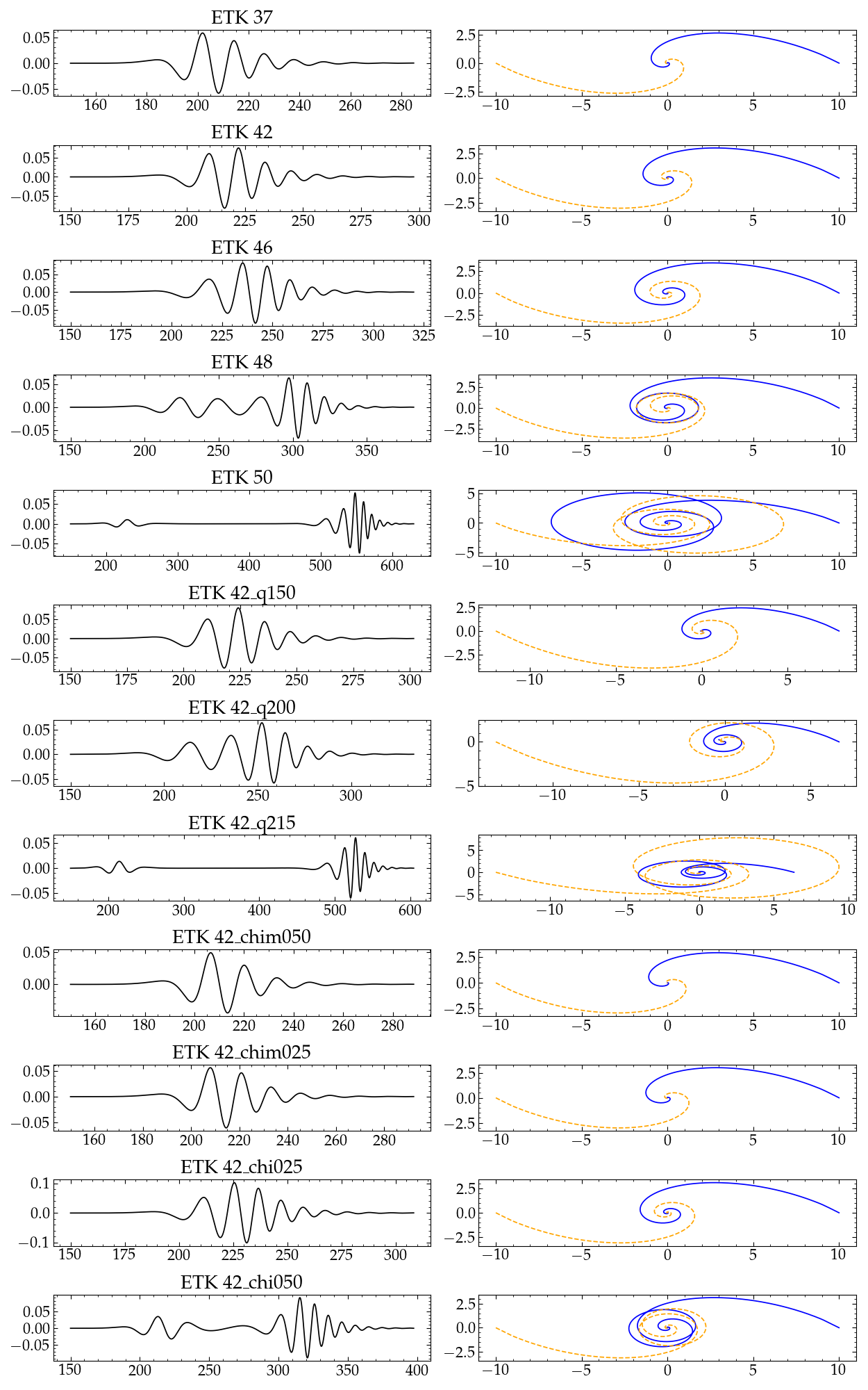
Appendix A Puncture tracks and $\psi_{4}$

In this Appendix we gather the unprocessed data for $\psi_{4}$ extracted at $R=100M$ and the corresponding puncture trajectories for all simulations. This information is collected in Fig. 11.

Figure 11: Puncture tracks and $\psi_{4}^{(2,2)}$ for all EinsteinToolkit simulations

Appendix B NR technical information

B.1 Code comparison for $\psi_{4}$

This appendix shows the comparison between the leading modes of $\psi_{4}$ obtained from EinsteinToolkit and GR-Athena++ simulations without using extrapolation. Note that this is the data obtained directly from our numerics, so this is a direct comparison between both codes. We write the leading mode of $\psi_{4}$ in terms of its phase and shift by

$$\psi_{4}(t)=a(t)e^{i\tilde{\phi}(t)}$$ (25)

We show our results for the differences in Fig. 12, and gather the results for the differences at merger in Table 6.

Table 6: [Amplitude and phase differences at merger for the leading mode of $\psi_{4}$ in simulations ETK42q1s0,48q1s0,50q1s0, GRA42q1s0,48q1s0,50q1s0 carried out at low, medium, and high resolutions, as listed in Table 2.]

ID	res	$\Delta a_{{\rm mrg}}^{GRA\,ETK}/a^{ETK}$	$\Delta\tilde{\phi}_{{\rm mrg}}^{GRA\,ETK}$
	L	$9.610\cdot 10^{-3}$	$2.179\cdot 10^{-2}$
42q1s0	M	$1.612\cdot 10^{-2}$	$1.833\cdot 10^{-2}$
	H	$1.728\cdot 10^{-2}$	$1.535\cdot 10^{-2}$
	L	$1.826\cdot 10^{-2}$	$1.592\cdot 10^{-1}$
48q1s0	M	$1.963\cdot 10^{-2}$	$2.253\cdot 10^{-2}$
	H	$1.834\cdot 10^{-2}$	$5.373\cdot 10^{-3}$
	L	$1.817\cdot 10^{-2}$	$6.526\cdot 10^{-1}$
50q1s0	M	$1.791\cdot 10^{-2}$	$7.651\cdot 10^{-2}$
	H	$1.761\cdot 10^{-2}$	$7.139\cdot 10^{-3}$

Figure 12: Comparison between EinsteinToolkit and GR-Athena++ simulations ETK50 and GRA50 at fixed resolution. We display the absolute value of the difference in normalized amplitude and phase of the non-extrapolated $\psi_{4}$ for every available resolution.

Appendix C Extra EOB/NR plots

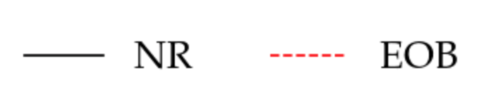
In this appendix we gather plots for the EOB/NR comparisons for the leading modes of the strain for all of our EinsteinToolkit simulations. The EOB model includes all of the NR information discussed in the main text, i.e. ring-down, and NQC corrections. We show our results for the real part of $h$, the modes frequencies, and the binding energy versus dimensionless angular momentum.

Figure 13: EOB/NR comparison plots for the real parts of the waveforms for the leading $(2,2)$ modes, normalized by $\nu$. In the EOB case, we plot the fully NR-informed model, including ringdown and NQC parameters.

Figure 14: EOB/NR comparison plots for the frequency of the leading $(2,2)$ modes. In the EOB case, we plot the fully NR-informed model, including ringdown and NQC parameters.

Figure 15: Binding energy versus dimensionless angular momentum curves for all simulations. The blue marker denotes the NR merger value for each dataset.

References

- Aasi et al. (2015) J. Aasi et al. (LIGO Scientific), Class. Quant. Grav. 32, 074001 (2015), arXiv:1411.4547 [gr-qc] .
- Acernese et al. (2015) F. Acernese et al. (VIRGO), Class. Quant. Grav. 32, 024001 (2015), arXiv:1408.3978 [gr-qc] .
- Akutsu et al. (2021) T. Akutsu et al. (KAGRA), PTEP 2021, 05A101 (2021), arXiv:2005.05574 [physics.ins-det] .
- Abbott et al. (2021) R. Abbott et al. (LIGO Scientific, VIRGO, KAGRA), (2021), arXiv:2111.03606 [gr-qc] .
- Abbott et al. (2020a) R. Abbott et al. (LIGO Scientific, Virgo), Phys. Rev. Lett. 125, 101102 (2020a), arXiv:2009.01075 [gr-qc] .
- Abbott et al. (2020b) R. Abbott et al. (LIGO Scientific, Virgo), Astrophys. J. Lett. 900, L13 (2020b), arXiv:2009.01190 [astro-ph.HE] .
- Gamba et al. (2022) R. Gamba, M. Breschi, G. Carullo, P. Rettegno, S. Albanesi, S. Bernuzzi, and A. Nagar, Nat. Astron. (2022), 10.1038/s41550-022-01813-w, arXiv:2106.05575 [gr-qc] .
- Romero-Shaw et al. (2020) I. M. Romero-Shaw, P. D. Lasky, E. Thrane, and J. C. Bustillo, Astrophys. J. Lett. 903, L5 (2020), arXiv:2009.04771 [astro-ph.HE] .
- Bustillo et al. (2021) J. C. Bustillo, N. Sanchis-Gual, A. Torres-Forné, J. A. Font, A. Vajpeyi, R. Smith, C. Herdeiro, E. Radu, and S. H. W. Leong, Phys. Rev. Lett. 126, 081101 (2021), arXiv:2009.05376 [gr-qc] .
- Gayathri et al. (2022) V. Gayathri, J. Healy, J. Lange, B. O’Brien, M. Szczepanczyk, I. Bartos, M. Campanelli, S. Klimenko, C. O. Lousto, and R. O’Shaughnessy, Nature Astron. 6, 344 (2022), arXiv:2009.05461 [astro-ph.HE] .
- Shibata et al. (2021) M. Shibata, K. Kiuchi, S. Fujibayashi, and Y. Sekiguchi, Phys. Rev. D 103, 063037 (2021), arXiv:2101.05440 [astro-ph.HE] .
- Rasskazov and Kocsis (2019) A. Rasskazov and B. Kocsis, Astrophys. J. 881, 20 (2019), arXiv:1902.03242 [astro-ph.HE] .
- Tagawa et al. (2020) H. Tagawa, Z. Haiman, and B. Kocsis, Astrophys. J. 898, 25 (2020), arXiv:1912.08218 [astro-ph.GA] .
- Zevin et al. (2019) M. Zevin, J. Samsing, C. Rodriguez, C.-J. Haster, and E. Ramirez-Ruiz, Astrophys. J. 871, 91 (2019), arXiv:1810.00901 [astro-ph.HE] .
- Samsing and D’Orazio (2018) J. Samsing and D. J. D’Orazio, Mon. Not. Roy. Astron. Soc. 481, 5445 (2018), arXiv:1804.06519 [astro-ph.HE] .
- Nagar et al. (2021a) A. Nagar, P. Rettegno, R. Gamba, and S. Bernuzzi, Phys. Rev. D 103, 064013 (2021a), arXiv:2009.12857 [gr-qc] .
- East et al. (2013) W. E. East, S. T. McWilliams, J. Levin, and F. Pretorius, Phys. Rev. D87, 043004 (2013), arXiv:1212.0837 [gr-qc] .
- Loutrel (2020) N. Loutrel, (2020), arXiv:2009.11332 [gr-qc] .
- O’Leary et al. (2009) R. M. O’Leary, B. Kocsis, and A. Loeb, Monthly Notices of the Royal Astronomical Society 395, 2127 (2009), https://academic.oup.com/mnras/article-pdf/395/4/2127/2931749/mnras0395-2127.pdf .
- Amaro-Seoane (2018) P. Amaro-Seoane, Phys. Rev. D 98, 063018 (2018), arXiv:1807.03824 [astro-ph.HE] .
- Punturo et al. (2010) M. Punturo, M. Abernathy, F. Acernese, B. Allen, N. Andersson, et al., Class.Quant.Grav. 27, 084007 (2010).
- Mukherjee et al. (2020) S. Mukherjee, S. Mitra, and S. Chatterjee, (2020), arXiv:2010.00916 [gr-qc] .
- Gold and Brügmann (2013) R. Gold and B. Brügmann, Phys. Rev. D88, 064051 (2013), arXiv:1209.4085 [gr-qc] .
- Nelson et al. (2019) P. E. Nelson, Z. B. Etienne, S. T. McWilliams, and V. Nguyen, Phys. Rev. D 100, 124045 (2019), arXiv:1909.08621 [gr-qc] .
- Bae et al. (2020) Y.-B. Bae, H. M. Lee, and G. Kang, Astrophys. J. 900, 175 (2020), arXiv:2007.14019 [gr-qc] .
- Jaraba and Garcia-Bellido (2021) S. Jaraba and J. Garcia-Bellido, Phys. Dark Univ. 34, 100882 (2021), arXiv:2106.01436 [gr-qc] .
- Healy and Lousto (2022) J. Healy and C. O. Lousto, Phys. Rev. D 105, 124010 (2022), arXiv:2202.00018 [gr-qc] .
- Damour and Nagar (2014) T. Damour and A. Nagar, Phys.Rev. D90, 024054 (2014), arXiv:1406.0401 [gr-qc] .
- Bernuzzi et al. (2015) S. Bernuzzi, A. Nagar, T. Dietrich, and T. Damour, Phys.Rev.Lett. 114, 161103 (2015), arXiv:1412.4553 [gr-qc] .
- Nagar et al. (2017) A. Nagar, G. Riemenschneider, and G. Pratten, Phys. Rev. D96, 084045 (2017), arXiv:1703.06814 [gr-qc] .
- Nagar et al. (2018) A. Nagar et al., Phys. Rev. D98, 104052 (2018), arXiv:1806.01772 [gr-qc] .
- Akcay et al. (2019) S. Akcay, S. Bernuzzi, F. Messina, A. Nagar, N. Ortiz, and P. Rettegno, Phys. Rev. D99, 044051 (2019), arXiv:1812.02744 [gr-qc] .
- Nagar et al. (2019) A. Nagar, G. Pratten, G. Riemenschneider, and R. Gamba, (2019), arXiv:1904.09550 [gr-qc] .
- Nagar et al. (2020) A. Nagar, G. Riemenschneider, G. Pratten, P. Rettegno, and F. Messina, Phys. Rev. D 102, 024077 (2020), arXiv:2001.09082 [gr-qc] .
- Chiaramello and Nagar (2020) D. Chiaramello and A. Nagar, Phys. Rev. D 101, 101501 (2020), arXiv:2001.11736 [gr-qc] .
- Nagar et al. (2021b) A. Nagar, A. Bonino, and P. Rettegno, Phys. Rev. D 103, 104021 (2021b), arXiv:2101.08624 [gr-qc] .
- Nagar and Rettegno (2021) A. Nagar and P. Rettegno, Phys. Rev. D 104, 104004 (2021), arXiv:2108.02043 [gr-qc] .
- Iglesias et al. (2022) H. L. Iglesias et al., (2022), arXiv:2208.01766 [gr-qc] .
- Damour et al. (2014) T. Damour, F. Guercilena, I. Hinder, S. Hopper, A. Nagar, and L. Rezzolla, Phys. Rev. D 89, 081503 (2014), arXiv:1402.7307 [gr-qc] .
- Hopper et al. (2022) S. Hopper, A. Nagar, and P. Rettegno, (2022), arXiv:2204.10299 [gr-qc] .
- Damour and Rettegno (2022) T. Damour and P. Rettegno, (2022), arXiv:2211.01399 [gr-qc] .
- Albertini et al. (2021) A. Albertini, A. Nagar, P. Rettegno, S. Albanesi, and R. Gamba, (2021), arXiv:2111.14149 [gr-qc] .
- Albertini et al. (2022a) A. Albertini, A. Nagar, A. Pound, N. Warburton, B. Wardell, L. Durkan, and J. Miller, Phys. Rev. D 106, 084061 (2022a), arXiv:2208.01049 [gr-qc] .
- Albertini et al. (2022b) A. Albertini, A. Nagar, A. Pound, N. Warburton, B. Wardell, L. Durkan, and J. Miller, Phys. Rev. D 106, 084062 (2022b), arXiv:2208.02055 [gr-qc] .
- Albanesi et al. (2021) S. Albanesi, A. Nagar, and S. Bernuzzi, Phys. Rev. D 104, 024067 (2021), arXiv:2104.10559 [gr-qc] .
- Albanesi et al. (2022a) S. Albanesi, A. Nagar, S. Bernuzzi, A. Placidi, and M. Orselli, Phys. Rev. D 105, 104031 (2022a), arXiv:2202.10063 [gr-qc] .
- Morrás et al. (2022) G. Morrás, J. García-Bellido, and S. Nesseris, Phys. Dark Univ. 35, 100932 (2022), arXiv:2110.08000 [astro-ph.HE] .
- Ebersold et al. (2022) M. Ebersold, S. Tiwari, L. Smith, Y.-B. Bae, G. Kang, D. Williams, A. Gopakumar, I. S. Heng, and M. Haney, (2022), arXiv:2208.07762 [gr-qc] .
- Löffler et al. (2012) F. Löffler et al., Class. Quant. Grav. 29, 115001 (2012), arXiv:1111.3344 [gr-qc] .
- Brandt and Brügmann (1997) S. Brandt and B. Brügmann, Phys. Rev. Lett. 78, 3606 (1997), arXiv:gr-qc/9703066 .
- Ansorg et al. (2004) M. Ansorg, B. Brügmann, and W. Tichy, Phys. Rev. D70, 064011 (2004), arXiv:gr-qc/0404056 .
- Baumgarte and Shapiro (1999) T. W. Baumgarte and S. L. Shapiro, Phys. Rev. D59, 024007 (1999), arXiv:gr-qc/9810065 .
- Shibata and Nakamura (1995) M. Shibata and T. Nakamura, Phys. Rev. D52, 5428 (1995).
- Daszuta et al. (2021) B. Daszuta, F. Zappa, W. Cook, D. Radice, S. Bernuzzi, and V. Morozova, Astrophys. J. Supp. 257, 25 (2021), arXiv:2101.08289 [gr-qc] .
- Bona et al. (2003) C. Bona, T. Ledvinka, C. Palenzuela, and M. Zacek, Phys. Rev. D67, 104005 (2003), arXiv:gr-qc/0302083 .
- Pretorius and Khurana (2007) F. Pretorius and D. Khurana, Class.Quant.Grav. 24, S83 (2007), arXiv:gr-qc/0702084 [GR-QC] .
- Lousto et al. (2010) C. O. Lousto, H. Nakano, Y. Zlochower, and M. Campanelli, Phys.Rev. D82, 104057 (2010), arXiv:1008.4360 [gr-qc] .
- Nakano (2015) H. Nakano, Class. Quant. Grav. 32, 177002 (2015), arXiv:1501.02890 [gr-qc] .
- Reisswig and Pollney (2011) C. Reisswig and D. Pollney, Class.Quant.Grav. 28, 195015 (2011), arXiv:1006.1632 [gr-qc] .
- Damour et al. (2012) T. Damour, A. Nagar, D. Pollney, and C. Reisswig, Phys.Rev.Lett. 108, 131101 (2012), arXiv:1110.2938 [gr-qc] .
- Nagar et al. (2016) A. Nagar, T. Damour, C. Reisswig, and D. Pollney, Phys. Rev. D93, 044046 (2016), arXiv:1506.08457 [gr-qc] .
- Bernuzzi et al. (2012a) S. Bernuzzi, A. Nagar, M. Thierfelder, and B. Brügmann, Phys.Rev. D86, 044030 (2012a), arXiv:1205.3403 [gr-qc] .
- Bernuzzi et al. (2014) S. Bernuzzi, T. Dietrich, W. Tichy, and B. Brügmann, Phys.Rev. D89, 104021 (2014), arXiv:1311.4443 [gr-qc] .
- Bernuzzi et al. (2012b) S. Bernuzzi, M. Thierfelder, and B. Brügmann, Phys.Rev. D85, 104030 (2012b), arXiv:1109.3611 [gr-qc] .
- Brügmann et al. (2008) B. Brügmann, J. A. Gonzalez, M. Hannam, S. Husa, U. Sperhake, et al., Phys.Rev. D77, 024027 (2008), arXiv:gr-qc/0610128 [gr-qc] .
- Riemenschneider et al. (2021) G. Riemenschneider, P. Rettegno, M. Breschi, A. Albertini, R. Gamba, S. Bernuzzi, and A. Nagar, Phys. Rev. D 104, 104045 (2021), arXiv:2104.07533 [gr-qc] .
- Buonanno and Damour (1999) A. Buonanno and T. Damour, Phys. Rev. D59, 084006 (1999), arXiv:gr-qc/9811091 .
- Buonanno et al. (2006) A. Buonanno, Y. Chen, and T. Damour, Phys. Rev. D74, 104005 (2006), arXiv:gr-qc/0508067 .
- Bonino et al. (2023) A. Bonino, R. Gamba, P. Schmidt, A. Nagar, G. Pratten, M. Breschi, P. Rettegno, and S. Bernuzzi, Phys. Rev. D 107, 064024 (2023), arXiv:2207.10474 [gr-qc] .
- Khalil et al. (2021) M. Khalil, A. Buonanno, J. Steinhoff, and J. Vines, Phys. Rev. D 104, 024046 (2021), arXiv:2104.11705 [gr-qc] .
- Placidi et al. (2022) A. Placidi, S. Albanesi, A. Nagar, M. Orselli, S. Bernuzzi, and G. Grignani, Phys. Rev. D 105, 104030 (2022), arXiv:2112.05448 [gr-qc] .
- Albanesi et al. (2022b) S. Albanesi, A. Placidi, A. Nagar, M. Orselli, and S. Bernuzzi, Phys. Rev. D 105, L121503 (2022b), arXiv:2203.16286 [gr-qc] .
- Berti et al. (2006) E. Berti, V. Cardoso, and C. M. Will, Phys. Rev. D73, 064030 (2006), arXiv:gr-qc/0512160 .
- Virtanen et al. (2020) P. Virtanen, R. Gommers, T. E. Oliphant, M. Haberland, T. Reddy, D. Cournapeau, E. Burovski, P. Peterson, W. Weckesser, J. Bright, S. J. van der Walt, M. Brett, J. Wilson, K. J. Millman, N. Mayorov, A. R. J. Nelson, E. Jones, R. Kern, E. Larson, C. J. Carey, İ. Polat, Y. Feng, E. W. Moore, J. VanderPlas, D. Laxalde, J. Perktold, R. Cimrman, I. Henriksen, E. A. Quintero, C. R. Harris, A. M. Archibald, A. H. Ribeiro, F. Pedregosa, P. van Mulbregt, and SciPy 1.0 Contributors, Nature Methods 17, 261 (2020).
- Walther et al. (2009) B. Walther, B. Brügmann, and D. Müller, Phys.Rev. D79, 124040 (2009), arXiv:0901.0993 [gr-qc] .
- (76) “Updated Advanced LIGO sensitivity design curve,” https://dcc.ligo.org/LIGO-T1800044/public.
- Nitz et al. (2022) A. Nitz, I. Harry, D. Brown, C. M. Biwer, J. Willis, T. D. Canton, C. Capano, T. Dent, L. Pekowsky, A. R. Williamson, S. De, M. Cabero, B. Machenschalk, D. Macleod, P. Kumar, F. Pannarale, S. Reyes, G. S. C. Davies, dfinstad, S. Kumar, M. Tápai, L. Singer, S. Khan, S. Fairhurst, A. Nielsen, S. Singh, T. Massinger, K. Chandra, shasvath, and veronica villa, “gwastro/pycbc: v2.0.5 release of pycbc,” (2022).
- Abrahams and Price (1996) A. M. Abrahams and R. H. Price, Phys. Rev. D53, 1963 (1996), gr-qc/9508059 .
- Nagar and Rezzolla (2005) A. Nagar and L. Rezzolla, Class. Quant. Grav. 22, R167 (2005), arXiv:gr-qc/0502064 .
- Pazos et al. (2007) E. Pazos et al., Class. Quant. Grav. 24, S341 (2007), gr-qc/0612149 .
- Buonanno et al. (2009) A. Buonanno, Y. Pan, H. P. Pfeiffer, M. A. Scheel, L. T. Buchman, and L. E. Kidder, Phys. Rev. D 79, 124028 (2009), arXiv:0902.0790 [gr-qc] .
- Bishop et al. (2009) N. T. Bishop, C. Reisswig, D. Pollney, and B. Szilagyi, in 12th Marcel Grossmann Meeting on General Relativity (2009) pp. 816–819.
- Reisswig et al. (2009) C. Reisswig, N. Bishop, D. Pollney, and B. Szilagyi, Phys.Rev.Lett. 103, 221101 (2009), arXiv:0907.2637 [gr-qc] .
- Reisswig et al. (2010) C. Reisswig, N. T. Bishop, D. Pollney, and B. Szilagyi, Class. Quant. Grav. 27, 075014 (2010), arXiv:0912.1285 [gr-qc] .
- Calderon Bustillo et al. (2022) J. Calderon Bustillo, I. C. F. Wong, N. Sanchis-Gual, S. H. W. Leong, A. Torres-Forne, K. Chandra, J. A. Font, C. Herdeiro, E. Radu, and T. G. F. Li, (2022), arXiv:2205.15029 [gr-qc] .
- Ossokine et al. (2018) S. Ossokine, T. Dietrich, E. Foley, R. Katebi, and G. Lovelace, Phys. Rev. D98, 104057 (2018), arXiv:1712.06533 [gr-qc] .